great lakes coastal hazard study - midcoast council€¦ · great lakes coastal hazard study...

Great Lakes Coastal Hazard Study

Appendix C – Climate Change

For: Great Lakes Council

Project Name: Great Lakes Coastal Hazard Study

Project Number: 3001829

Report for: Great Lakes Council

PREPARATION, REVIEW AND AUTHORISATION

Revision # Date Prepared by Reviewed by Approved for Issue by

1 22/08/2012 M. Glatz, A. Xiao C. Adamantidis D. Messiter

ISSUE REGISTER

Distribution List Date Issued Number of Copies

Great Lakes Council: 22/08/2012 1 (E)

SMEC staff:

Associates:

Sydney Office Library (SMEC office location):

SMEC Project File: 22/08/12 1

SMEC COMPANY DETAILS

SMEC Australia Pty Ltd

PO Box 1346, Newcastle NSW 2300

Tel: 02 4925 9600

Fax: 02 4925 3888

Email: [email protected]

www.smec.com

The information within this document is and shall remain the property of SMEC Australia Pty Ltd

http://www.smec.com/

Great Lakes Coastal Hazard Study 3001829 | Revision No. 1 | Page | i

TABLE OF CONTENTS

1 INTRODUCTION .............................................................................................. 1

2 BEACH ROTATION ......................................................................................... 2

2.1 Introduction ....................................................................................................... 2

2.2 Previous Studies ............................................................................................... 2

2.3 Causes of Beach Rotation ................................................................................. 2

2.4 Beach Rotation and Longshore Drift at Great Lakes .......................................... 3

3 SEA LEVEL RISE............................................................................................. 6

3.1 Historic Sea Level Rise ..................................................................................... 6

3.2 Projected Sea Level Rise .................................................................................. 6

3.2.1 NSW Sea Level Rise Policy Statement ...................................................... 8

3.3 Impacts of Sea Level Rise ................................................................................. 9

3.3.1 Bruun Rule ................................................................................................. 9

3.3.2 Analytical Determination of Bruun Rule Parameters ................................... 9

3.3.3 Nearshore geological survey .................................................................... 12

3.3.4 Sensitivity Analysis ................................................................................... 12

3.3.5 Beach Response ...................................................................................... 13

3.3.6 Estuary Entrance Response ..................................................................... 15

4 INCREASED STORMINESS .......................................................................... 16

5 SUMMARY AND CONCLUSIONS ................................................................. 17

REFERENCES ..................................................................................................... 18

FIGURES ............................................................................................................. 20

Great Lakes Coastal Hazard Study 3001829 | Revision No. 1 | Page | ii

LIST OF TABLES

Table C1: Beach rotation results at the main beaches along Great Lakes Council coastline

Table C2 : Range of Sea Level Rise predictions (IPCC 2007)

Table C3: Contributions to global average sea level rise for various scenarios, 1990 – 2095 (source: IPCC 2007)

Table C4: Projected Greenhouse sea level rise scenarios for Great Lakes coastline

Table C5: Determination of the berm height, the closure depth and the profile length per block and per continuous beach from bathymetric and topographic data

Table C6: Predicted beach erosion due to sea level rise

LIST OF FIGURES

Figure C1: Wave rotation caused by El-Niño or La-Niña mean states (after Goodwin et al. 2007)

Figure C2: Example of change in nearshore angle caused by change in offshore wave approach angle from 127°TN to 140°TN at Number One Beach

Figure C3: Measured global mean sea level 1870 – 2002 (White and Church, 2006)

Figure C4: IPCC (2001) Sea level rise estimates

Figure C5: IPCC (2007) Global average sea level rise estimates

Figure C6: Concept of shoreline recession due to sea level rise

Figure C7: Result of the sediment size analysis

Figure C8: Suggested relationship for shape factor A vs. grain size D

Figure C9: Nearshore profile at Boat Beach vs. idealised equilibrium profile

Figure C10: Impact of climate change on wind speeds along NSW coast (Hennessy, 2004)

Great Lakes Coastal Hazard Study 3001829 | Revision No. 1 | Page | 1

1 INTRODUCTION

Climate is the pattern or cycle of weather conditions, such as temperature, wind, rain, snowfall, humidity, clouds, including extreme or occasional ones, over a large area and averaged over many years. Changes to the climate and, specifically, changes in mean sea levels, wind conditions, wave energy and wave direction, can be such as to change the coastal sediment transport processes shaping beach alignments.

Climate change had been defined broadly by the Intergovernmental Panel on Climate Change (IPCC, 2001) as any change in climate over time whether due to natural variability or as a result of human activity. Apart from the expected climate variability reflected in seasonal changes, storms, etc., climate changes that are considered herein refer to the variability in average trends in weather that may occur over time periods of decades and centuries. These may be a natural variability of decadal oscillation or permanent trends that may result from such factors as changes in solar activity, long-period changes in the Earth's orbital elements (eccentricity, obliquity of the ecliptic, precession of equinoxes), or man-made factors such as, for example, increasing atmospheric concentrations of carbon dioxide and other greenhouse gases.

The signature of climate variability over periods of decades is seen in the Southern Oscillation Index (SOI), a number calculated from the monthly or seasonal fluctuations in the air pressure difference between Tahiti and Darwin. Sustained negative values of the SOI usually are accompanied by sustained warming of the central and eastern tropical Pacific Ocean, a decrease in the strength of the Pacific Trade Winds and a reduction in rainfall over eastern and northern Australia. This is called an El-Niño episode. During these episodes, a more benign south-easterly wave condition is expected on the NSW coast. Positive values of the SOI are associated with stronger Pacific trade winds and warmer sea temperatures to the north of Australia, popularly known as a La-Niña episode. Waters in the central and eastern tropical Pacific Ocean become cooler during this time. Together, these give an increased probability that eastern and northern Australia will be wetter than normal and, during these episodes, severe storms may be expected on the Australian Eastern seaboard.

Over much longer time frames, the Intergovernmental Panel on Climate Change (IPCC 2001) has indicated that the global average surface temperature has increased over the 20th century by 0.6°C and that this warming will continue at an accelerating rate. This warming of the average surface temperature is postulated to lead to warming of the oceans, which would lead to thermal expansion of the oceans and loss of mass from land-based ice sheets and glaciers. This would lead to a sea level rise which, in turn, would lead to recession of unconsolidated shorelines.

http://www.bom.gov.au/climate/glossary/elnino.shtml

http://www.bom.gov.au/climate/glossary/trade_winds.shtml

http://www.bom.gov.au/climate/glossary/lanina.shtml


2 BEACH ROTATION

2.1 Introduction

Studies of embayed beaches on the NSW coast have identified a sensitivity of shoreline alignment to mean wave direction, which has been linked to the Southern Oscillation Index (SOI). Since 1876, the maximum value of the monthly average of the SOI that has been recorded was +34.8 in August 1917. For much of that year the monthly average of the SOI was above +20 and several very severe storms were experienced along the entire NSW coast from June to November that year. January – May 1974, the monthly average of the SOI varied from around +20 to +10, which may have been relevant to the occurrence of the severe storms of May − June 1974.

Goodwin (2005) demonstrated that, since the 1880s, the monthly mid-shelf mean wave direction (MWD) for southeastern Australia has varied from around 125°T to 145°T with a strong annual cycle coupled to mean, spectral-peak wave period. Months and years when a more southerly MWD occurs are accompanied by an increase in the spectral-peak wave period. The most significant multi-decadal fluctuation in the time series was from 1894 to 1914, when Tasman Sea surface temperatures (SST) were 1°–1.5°C cooler, monthly and annual wave directions were up to 4°–5° more southerly and, by inference, spectral-peak wave periods were longer when compared with the series since 1915. The sustained shift in wave direction would have had a significant influence on beach and coastal compartment alignment along the NSW coast (Goodwin, 2005).

2.2 Previous Studies

Studies of beach rotation as a result of variations in the SOI have been undertaken at Narrabeen Beach and Palm Beach (Short et al., 2000; Ranasinghe et al., 2004). Data from Ranasinghe (et al., 2004) indicated an anti-clockwise rotation of these beaches as a result of a positive value in the SOI and vice versa. A sustained SOI of +10 to +20 (a La-Niña episode) resulted in an anti-clockwise rotation of Narrabeen Beach by around 0.9° and a sustained SOI of around +15 to +26 resulted in a similar rotation of Palm Beach by around 0.7°. On the other hand, a sustained SOI of −10 to −16 (an El-Niño episode) resulted in a clockwise rotation of Narrabeen Beach by around 1.2° and a sustained SOI of −25 to −38 resulted in a clockwise rotation of Palm Beach by around 0.7°.

These rotations were reflected in the translation of the mean waterline or swash zone of the beach berm and they did not affect the dune alignment. Analysis of 23 years of monthly profiles at Narrabeen Beach showed that rotations accounted for up to 15 m and some 30 m3/m (above MSL) of the shore-normal beach sand exchange (Short et al., 2000). At Palm Beach, the maximum recession of the swash zone that was recorded over the 2.5 year period was around 10 m (Ranasinghe et al., 2004), which represented the removal of around 20 m3/m of sub-aerial beach sand store at the extreme ends of the beach. For a given degree of beach rotation, greater recession or progradation of the swash zone and, hence, greater beach sand exchange would be expected on longer beaches.

2.3 Causes of Beach Rotation

These beach rotations were considered to be caused by changes to both the mean direction and magnitude of wave energy flux, the signature of which is reflected in the SOI. The larger magnitude of wave energy flux induced greater onshore/offshore sand transport whereas changes in direction affected also alongshore transport rates and directions.





Both Narrabeen Beach and Palm Beach are exposed open coast beaches and would experience the maximum shift in the mean direction of offshore wave energy flux. Sheltered embayments would not experience much rotation because the mean direction of wave energy flux cannot vary much. This is because the nearshore incident swell direction is controlled and limited by severe wave refraction with the beach already being aligned normal to the direction of the nearshore wave energy flux vector.

On open coast beaches, the La-Niña events, which are correlated to severe storms, may result in recession of the swash zone at the extreme northern ends of the beaches. This occurs rapidly following the SOI shift (a few months; Ranasinghe et al., 2004) and may result in reducing the available sand store on the beach that provides a buffer to the Beach erosion demand. However, as the concomitant accretion at the southern end of the beach lags the SOI trend shift considerably (by up to and in excess of 1 year; Ranasinghe et al., 2004), this obviates any advantage that the accreted swash zone may accrue to supplying the Beach erosion demand.

2.4 Beach Rotation and Longshore Drift at Great Lakes

There is no real evidence of beach rotation at the different beaches as similar trends of recession or progradation occurred along the entire beach length at the various locations.

Goodwin et al. (2007) identifies conceptual sediment transport processes based on mean wave climate states. A more southerly wave climate consistent with an El-Niño event would lead to greater northerly longshore sediment transport (clockwise beach rotation) while a more easterly wave climate would lead to an anti-clockwise translation (Figure C.1). A shift from dominant La-Niña to dominant El-Niño conditions caused by climate change would enhance northerly longshore drift and therefore increase the beach recession.

A wave refraction analysis was undertaken for various beaches along Great Lakes Council coastline to investigate the impact of change in offshore wave angle on mean wave angle in the nearshore area. This was undertaken using SWAN (acronym for

Simulating WAves Nearshore Cycle III version 40.11). SWAN is a numerical wave transformation program developed at the Delft University of Technology (Holthuijsen et al., 2000). SWAN can be used to describe wave transformation in shallow water and to obtain realistic estimates of wave parameters in coastal areas, lakes and estuaries from given wind, bathymetric and current conditions. The background to SWAN is provided in Young (1999) and Booij et al., (1999). SWAN has been validated using field data by Nielsen & Adamantidis (2003).

An example of change in nearshore angle caused by change in offshore wave approach angle from 127°TN to 140°TN at Number One Beach is provided in Figure C.2.

The range of offshore wave angles examined was from 127°TN to 140°TN, corresponding to the annual Mean Wave Direction (MWD) reported by Goodwin (2005). Given the limited amount of available bathymetric data along Great Lakes LGA coastline (mostly limited to the 10 and 20 m isobaths), the nearshore angle resulting from the SWAN modelling would not be accurate. A variation in angle of around 0.5° has been found in previous studies of beach rotation along the east coast of New South Wales (Shoalhaven Coastal Hazard Study (SMEC 2008), Nambucca Coastal Hazard Study (SMEC 2010)). Therefore, this value was assumed for the different beaches located along Great Lakes Council coastline. The maximum variation in wave angle in the nearshore area of Great Lakes is provided in Table C.1 for the main beaches that could be influenced by beach rotation. As the beach planform is typically normal to the MWD, the beach rotation that would be expected would be of the same order, with the effects seen most greatly at the extreme southern and northern ends of the beaches.



Table C 1: Beach rotation results at the main beaches along Great Lakes Council coastline

Beach Name Distance from the Centre of the

Beach (m)

Approximate Potential Maximum Beach Fluctuation

(m)

Nine Mile / Tuncurry Beach 5500* ±50*

Main Beach 280 ±2

One Mile Beach 600 ±5

Seven Mile Beach 4800** ±40**

Number One Beach 550 ±5

Lighthouse Beach 950 ±8

Treachery Beach 900 ±8

Bennetts Beach 6900** ±60**

* the presence of the training wall at Wallis Lake entrance generates the creation of sand bars offshore of the entrance that reduce the variation in angle along the southern end of the beach and curved shape of this very long beach would reduce the maximum beach fluctuation

** curved shape of this very long beach and refraction effects from offshore islands would reduce the maximum beach fluctuation

Assuming that the beach can be approximated by a straight line, the beach fluctuations due to rotation are estimated by the following formula:

rdistR tan

Where: R = beach fluctuation in metres at the location of interest

dist = distance in metres from the centre of the beach

r = estimated change in nearshore wave angle in degrees.

Beach fluctuation could potentially have a significant impact at Hawks Nest (Bennetts Beach) as it could increase the risk of a storm causing breakthrough of the tombolo, changing the hydrodynamics of Port Stephens entrance and exposing Port Stephens beaches to ocean swell. It should be noted, however, that the beach fluctuation due to rotation is confined to the beach berm and does not impact the dune.

Beach rotation could also have a significant impact along Nine Mile Beach and Seven Mile Beach. Both beaches are relatively curved which would attenuate the maximum beach fluctuation. Beach rotation would be limited by the presence of the rock outcrops at the extremities of the beaches.

Given the short beach length and orientation of Elizabeth Beach, Shelly Beach and Boat Beach (i.e. facing north and subject to strongly refracted southerly waves), the beach rotation at these locations would be negligible.


The beach rotation of Pebbly Beach and Burgess Beach would also be negligible given the short length of these beaches.

The results provided in Table C.1 represent the potential maximum beach fluctuation between mean wave directions of 127°TN and 140°TN.

The beach rotation phenomenon would primarily impact the beach berm by generating longshore sediment movements and given the low value for most beaches, would not impact the dunes, and hence the location of the hazard lines calculated in Appendix D. The signature of beach rotation will already have been captured in the photogrammetric data used to determine the design Beach erosion demand.


3 SEA LEVEL RISE

3.1 Historic Sea Level Rise

Tidal gauge data show that over the 20th century global average sea level rose between 0.1 m and 0.2 m; that is, at an average rate of between 1 mm/y to 2 mm/y (IPCC, 2001). Mitchell et al. (2001) summarised observed sea level rise in Australia and the Pacific. Analysis of data from Fort Denison in Sydney showed that, between 1914 and 1997, the underlying trend in sea level rise has been an average increase in relative sea level of 0.86 mm/year (and 1.18 mm/year in Newcastle). However, it was noted that there was considerable variation in the data, which was due to processes acting at inter-decadal scales, such as the El-Niño Southern Oscillation phenomenon. Part of this (25 mm) was due to isostatic rebound inducing a rise of the land mass, which is occurring at a rate of 0.3 mm/year. Mitchell et al. (2001) corrected sea-level changes at Fort Denison to an average increase of 1.16 mm/year to account for this rate of post-glacial rebound.

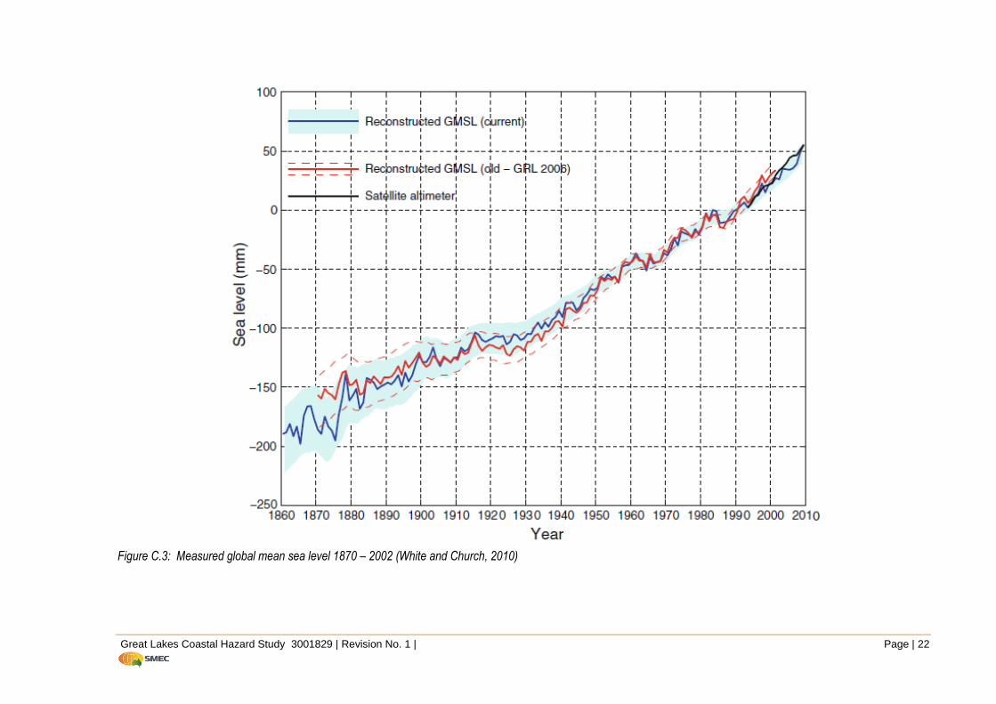
Satellite altimetry data has recently been employed to measure changes in global sea level – this has allowed a more accurate measurement of changes in Mean Sea Level around the globe since around 1993. From these measurements, it is apparent from Figure C.3 that the rate of sea level rise has accelerated in the later part of the 20th century, with sea level in Australia rising by around 3.2 ± 0.4 mm/year between 1993 and 2009 (Church and White, 2010).

3.2 Projected Sea Level Rise

The National Committee on Coastal and Ocean Engineering of Engineers Australia has issued Guidelines for Responding to the Effects of Climate Change in Coastal and Ocean Engineering (NCCOE, 2004). These Guidelines indicated a range of engineering estimates for global average sea level rise from 1990 to 2100 of 0.1 m to 0.9 m with a central value of 0.5 m. The Guidelines indicated also that global average sea level rise scenarios must be converted to estimated local relative sea level movement for each site. In this regard, reference has been made to the IPCC projections for global and regional sea level change.

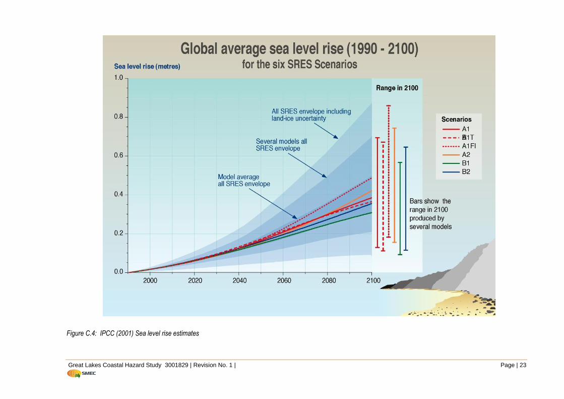
Using various climate models for different climate change scenarios, the Third Assessment Report (TAR) of the IPCC (2001) projected a range of sea level rises for the 21st century. It was projected that global average sea levels could rise from between 0.09 m and 0.88 m by 2100 (Figure C.4; and from between 0.05 m and 0.30 m by around 2055).

From the IPCC Fourth Assessment Report (2007), the 5% to 95% confidence limit ranges of sea level rise predictions for the 21st century are shown in Figure C.5 and summarised in Table C.2, for the various scenarios and based on the spread of model results.

It can be seen from Table C.2 that the 95% confidence interval for global average sea level rise in the worst case scenario (Scenario A1FI) is 0.59 m for the 2100 planning period. This is made up of various components, including thermal expansion of the oceans (the largest component), melting of the Greenland and Antarctic ice sheets and melting of land-based glaciers. There is considerable uncertainty also in the level of ice-sheet discharge, which could contribute, at a maximum, an additional 0.17 m to the worst-case scenario global average sea level rise (refer Table C.3). This would give an upper bound sea level rise of 0.76 m for the 2100 planning period.



There is also a local effect due to the East Australian Current, which could add around 10-14 cm to the global average sea level rise (McInnes et al.,2007).

In addition to the effects of climate change, there is also an existing underlying rate of sea level rise. Mitchell et al. (2001) quantified underlying rates of existing sea level rise at various tide gauge locations around Australia. Factors other than global warming that contribute to the underlying rate of sea level rise include (Walsh et al., 2004):

geological effects caused by the slow rebound of land that was covered by ice during the last Ice Age (isostatic rebound)

flooding of continental shelves since the end of the last Ice Age, which pushes down the shelves and causes the continent to push upwards in response (hydroisostasy)

changes in land height in tectonically or volcanically active regions

changes in atmospheric wind patterns and ocean currents

local subsidence due to sediment compaction or groundwater extraction

This underlying rate has been estimated at 0.12 m for 2100 in NSW.

Combining the relevant global and local information indicates that sea level rise on the NSW coast is expected to reach up to 0.90 m for the 2100 planning period. For 2050, the sea level rise benchmark advocated by the NSW Sea Level Rise Policy (2009) is 0.40 m.

It should be noted also that sea level rise is subject to considerable regional variation, with the southern ocean in general forecast to undergo less sea level rise than the Arctic, due to regional climatic variations and local changes in salinity and ocean density. In the region off the east coast of Australia, the IPCC (2007) report indicates that the expected sea level rise would be close to the geographic global average.

The NSW Office of Environment and Heritage (OEH) has recently been advocating sensitivity analyses using a range of sea level rise scenarios for various planning horizons. As the 5% lower bound estimate from the IPCC report has a 95% probability of being exceeded for the 2100 planning period it is generally excluded from the sensitivity analysis for planning purposes.

Table C 2: Range of Sea Level Rise Predictions (IPCC 2007)

Scenario 5% (Lower bound)

predicted sea level rise 1980-1999 to 2090-2099 (m)

Assumed median predicted sea level rise 1980-1999 to

2090-2099 (m)*

95% (upper bound) predicted sea level rise

1980-1999 to 2090-2099 (m)

B1 0.18 0.28 0.38

B2 0.20 0.32 0.43

A1B 0.21 0.35 0.48

A1T 0.20 0.33 0.45

A2 0.23 0.37 0.51

A1F1 0.26 0.43 0.59

* The IPCC (2007) report does not provide median values for predicted sea level rise. Median values have been assumed by adopting the central value between the 5% and 95% confidence interval limits.


Table C 3: Contributions to global average sea level rise for various scenarios, 1990 – 2095 (source: IPCC 2007).*

* The additional 0.17 m sea level rise allowed for uncertainties in ice-sheet discharge is the upper bound range under the A1FI scenario, as indicated in the Table. This needs to be added to the sea level rise attributed to the other sources of sea level rise indicated in Table 2, which include thermal ocean expansion, melting of glaciers and ice caps, melting of the Greenland Ice Sheet and changes in the Antarctic Ice Sheet.

The IPCC Fourth Assessment Report (2007) does not provide estimates of sea level rise for the 2050 planning horizon. However, the IPCC Third Assessment Report (2001) provides projections over the 21st century (Figure C.4), with a median value of around 0.2 m and a maximum value of around 0.35 m. Adding the underlying rates of sea level rise yields a maximum value of around 0.4 m for the 2050 planning period.

The projections of future sea level rise for the Great Lakes coastal hazard study are presented in Table C.4.

Table C 4: Projected Greenhouse sea level rise scenarios for Great Lakes coastline

Scenario Range\Year 2050* 2100*

Maximum 0.40 m 0.90 m

* Note – These values are estimated sea level rise relative to a 1990 baseline level.

3.2.1 NSW Sea Level Rise Policy Statement

The IPCC were unable to exclude larger values and there is emerging evidence in the current measurements and observations, suggesting the IPCC’s 2007 report may have underestimated the future rate of sea level rise. Therefore, the NSW Government through the NSW Sea Level Rise Policy Statement have set the NSW Sea Level Rise Planning benchmark at the upper bound levels of a 0.40 m increase above 1990 levels by 2050 and 0.90 m by 2100. The rationale behind the NSW Government’s adoption of the respective planning benchmark allowances for SLR are detailed in the DECCW publication “Derivation of the NSW Government’s sea level rise planning benchmarks – Technical Note (DECCW, 2009a). The benchmarks are based on the sea level rise developed by Australian and international experts and include globally averaged sea level rise, accelerated ice melt, and regional sea level rise variations.


3.3 Impacts of Sea Level Rise

3.3.1 Bruun Rule

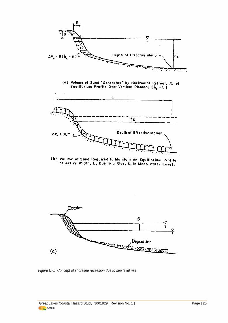
The most widely accepted method of estimating shoreline response to sea level rise is the Bruun Rule (Bruun, 1962; 1983). Bruun (1962, 1983) investigated the long term erosion along Florida’s beaches, which was assumed to be caused by a long term sea level rise. Bruun (1962, 1983) hypothesised that the beach assumed an equilibrium profile that kept pace with the rise in sea level without changing its shape, by an upward translation of sea level rise (S) and shoreline retreat (R).

Figure C.6 illustrates the concept of the Bruun Rule. The Bruun Rule equation is given by:

where: R = shoreline recession due to sea level rise;

S = sea level rise (m)

hc = closure depth

B = berm height; and

L = length of the active zone.

The Bruun model assumes that the beach profile is in an equilibrium state. It is noted that the depth of nearshore rock layers would mark the seaward extent of the equilibrium beach profile. Where the location and depth of nearshore rock is known, this has been taken into account in determining equilibrium profile slopes and length of the active zones for use in the Bruun Rule calculations.

Berm height is taken to be the average height of the dune along the beach, and closure depth is the depth at the seaward extent of measurable sand movement. The length of the active zone is the distance offshore along the profile in which sand movement still occurs.

3.3.2 Analytical Determination of Bruun Rule Parameters

Several schemas exist, based on analytical and laboratory studies, to determine closure depth and length of the active zone, including those of Swart (1974) and Hallermeier (1981, 1983).

Hallermeier (1981, 1983) defines a simple zonation of an onshore-offshore beach profile consisting of a littoral zone, shoal zone or buffer zone, and offshore zone where surface wave effects on the bed are negligible.

Based on an analytical approach, supported by laboratory data and some field data, the two water depths bounding the shoal zone, defined by ds and do are given by:

2

2

5.01

110

1

9.2

gTS

H

S

Hds

LBh

SR

c /


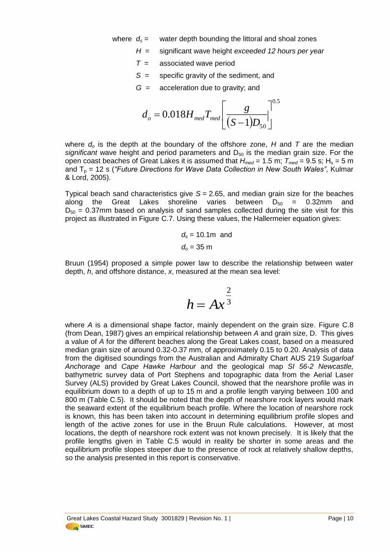
where ds = water depth bounding the littoral and shoal zones

H = significant wave height exceeded 12 hours per year

T = associated wave period

S = specific gravity of the sediment, and

G = acceleration due to gravity; and

where do is the depth at the boundary of the offshore zone, H and T are the median significant wave height and period parameters and D50 is the median grain size. For the open coast beaches of Great Lakes it is assumed that Hmed = 1.5 m; Tmed = 9.5 s; Hs = 5 m and Tp = 12 s (“Future Directions for Wave Data Collection in New South Wales”, Kulmar & Lord, 2005).

Typical beach sand characteristics give S = 2.65, and median grain size for the beaches along the Great Lakes shoreline varies between D50 = 0.32mm and D50 = 0.37mm based on analysis of sand samples collected during the site visit for this project as illustrated in Figure C.7. Using these values, the Hallermeier equation gives:

ds = 10.1m and

do = 35 m

Bruun (1954) proposed a simple power law to describe the relationship between water depth, h, and offshore distance, x, measured at the mean sea level:

3

2

Axh

where A is a dimensional shape factor, mainly dependent on the grain size. Figure C.8 (from Dean, 1987) gives an empirical relationship between A and grain size, D. This gives a value of A for the different beaches along the Great Lakes coast, based on a measured median grain size of around 0.32-0.37 mm, of approximately 0.15 to 0.20. Analysis of data from the digitised soundings from the Australian and Admiralty Chart AUS 219 Sugarloaf Anchorage and Cape Hawke Harbour and the geological map SI 56-2 Newcastle, bathymetric survey data of Port Stephens and topographic data from the Aerial Laser Survey (ALS) provided by Great Lakes Council, showed that the nearshore profile was in equilibrium down to a depth of up to 15 m and a profile length varying between 100 and 800 m (Table C.5). It should be noted that the depth of nearshore rock layers would mark the seaward extent of the equilibrium beach profile. Where the location of nearshore rock is known, this has been taken into account in determining equilibrium profile slopes and length of the active zones for use in the Bruun Rule calculations. However, at most locations, the depth of nearshore rock extent was not known precisely. It is likely that the profile lengths given in Table C.5 would in reality be shorter in some areas and the equilibrium profile slopes steeper due to the presence of rock at relatively shallow depths, so the analysis presented in this report is conservative.

5.0

501018.0

DS

gTHd medmedo


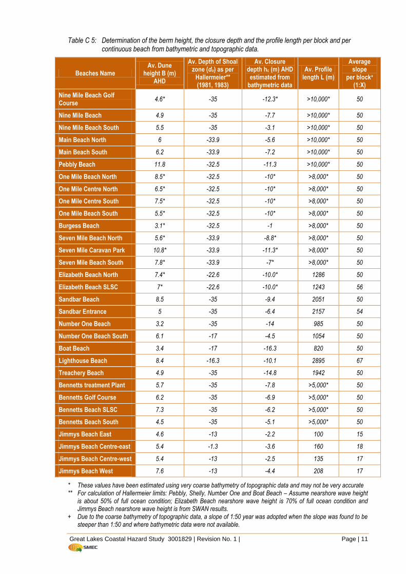
Table C 5: Determination of the berm height, the closure depth and the profile length per block and per continuous beach from bathymetric and topographic data.

Beaches Name Av. Dune

height B (m) AHD

Av. Depth of Shoal zone (do) as per

Hallermeier** (1981, 1983)

Av. Closure depth hc (m) AHD estimated from

bathymetric data

Av. Profile length L (m)

Average slope

per block+

(1:X)

Nine Mile Beach Golf Course

4.6* -35 -12.3* >10,000* 50

Nine Mile Beach 4.9 -35 -7.7 >10,000* 50

Nine Mile Beach South 5.5 -35 -3.1 >10,000* 50

Main Beach North 6 -33.9 -5.6 >10,000* 50

Main Beach South 6.2 -33.9 -7.2 >10,000* 50

Pebbly Beach 11.8 -32.5 -11.3 >10,000* 50

One Mile Beach North 8.5* -32.5 -10* >8,000* 50

One Mile Centre North 6.5* -32.5 -10* >8,000* 50

One Mile Centre South 7.5* -32.5 -10* >8,000* 50

One Mile Beach South 5.5* -32.5 -10* >8,000* 50

Burgess Beach 3.1* -32.5 -1 >8,000* 50

Seven Mile Beach North 5.6* -33.9 -8.8* >8,000* 50

Seven Mile Caravan Park 10.8* -33.9 -11.3* >8,000* 50

Seven Mile Beach South 7.8* -33.9 -7* >8,000* 50

Elizabeth Beach North 7.4* -22.6 -10.0* 1286 50

Elizabeth Beach SLSC 7* -22.6 -10.0* 1243 56

Sandbar Beach 8.5 -35 -9.4 2051 50

Sandbar Entrance 5 -35 -6.4 2157 54

Number One Beach 3.2 -35 -14 985 50

Number One Beach South 6.1 -17 -4.5 1054 50

Boat Beach 3.4 -17 -16.3 820 50

Lighthouse Beach 8.4 -16.3 -10.1 2895 67

Treachery Beach 4.9 -35 -14.8 1942 50

Bennetts treatment Plant 5.7 -35 -7.8 >5,000* 50

Bennetts Golf Course 6.2 -35 -6.9 >5,000* 50

Bennetts Beach SLSC 7.3 -35 -6.2 >5,000* 50

Bennetts Beach South 4.5 -35 -5.1 >5,000* 50

Jimmys Beach East 4.6 -13 -2.2 100 15

Jimmys Beach Centre-east 5.4 -1.3 -3.6 160 18

Jimmys Beach Centre-west 5.4 -13 -2.5 135 17

Jimmys Beach West 7.6 -13 -4.4 208 17

* These values have been estimated using very coarse bathymetry of topographic data and may not be very accurate ** For calculation of Hallermeier limits: Pebbly, Shelly, Number One and Boat Beach – Assume nearshore wave height

is about 50% of full ocean condition; Elizabeth Beach nearshore wave height is 70% of full ocean condition and Jimmys Beach nearshore wave height is from SWAN results.

+ Due to the coarse bathymetry of topographic data, a slope of 1:50 year was adopted when the slope was found to be steeper than 1:50 and where bathymetric data were not available.


The closure depths and the equilibrium profile lengths have been assessed from calculation of the Hallermeier zonation limits examination of bathymetry as well as the beach profile graphs. These two characteristics are the coordinates of the last point fitting with the equilibrium profile.

A comparison plot of the shore-normal profile at Boat Beach and the estimated equilibrium profile is given in Figure C.9 as an example of the assessment undertaken.

This analytical approach indicates steeper slopes of approximately 1:15 for some of the sheltered beaches. For the open coast, active profile slopes determined using Hallermeier’s proposed zonations are closer to the range of 1:50 to 1:100 recommended for NSW beaches (DECCW, 2010).

A purely analytical application of the Bruun Rule requires a number of assumptions and incomplete data that introduce additional uncertainty. These include:

Beach and nearshore profiles that are in state of equilibrium;

Slope parameter (m=⅔) is that used in Dean’s equilibrium equation is based on European and US conditions and has not been verified for Australian conditions;

Nearshore wave heights; and

sediment grain size and distribution of sediment types; and

use of the coarse bathymetric maps.

The application of one (Hallermeier) technique is described above, however, there are a broad range of techniques available for estimating the closure depth and several (Hallermeier, Birkmeier, Rijkswaterstaat, USACE, Bruun etc.) idealised formulae for estimating closure depth, based on offshore wave statistics. All formulae provide differing results.

3.3.3 Nearshore geological survey

In order to provide more confidence in the results of analytical approaches a review of local information has been completed.

In May 1979 offshore sediments and seabed depths were collected by PWD in conjunction with the Geological Survey of NSW as part of an investigation into sand movements at the entrance to Wallis Lake and adjacent coastlines (PWD 1985). The survey comprised bathymetric profiling and sediment sampling offshore to depths of 65 m. While the full extent of the survey is not known, three profile runs were made off Boomerang Beach and reported in (PWD, 1985).

This data shows that the nearshore profile slope is fairly constant at 1:50 to a depth of about 40 m, seaward of which there is an abrupt steepening of the slope to 1:20 to a depth of 50 m. Seaward of the 55 m contour the inner shelf slope flatters out at aboit 1:130. A across this profile the sand grain varies from about 0.35 mm on the beach face, fining to 0.2 mm at 65 m water depth.

This data, while limited, suggests that a slope of 1:50 is appropriate for open coast beaches in the Great Lakes region. 1:50 is recommended as the slope to adopt in Bruun Rule application for this study.

3.3.4 Sensitivity Analysis

Given the uncertainty in the depth of closure and active profile slope, it appropriate to consider a sensitivity analysis for this element of the Bruun Rule. It is common for the active beach profile slope to fall in the order of 1:50 to 1:100 for the east coast of NSW.


The range of recession due to sea level rise then becomes R = 50 x S to 100 x S. It is therefore possible for the recession due to sea level rise to be up to double the amount determined using the adopted active beach slope of 1:50.

3.3.5 Beach Response

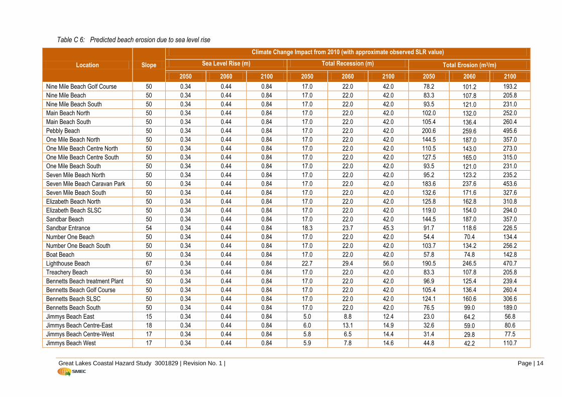
Results of the Bruun analysis are given in Table C.6. The 2050 and 2100 sea level rise benchmark of 0.40 m and 0.90 m from 1990 respectively, were adapted to include the measured sea level rise that already occurred between 1990 and 2011, which is around 0.06 m. Therefore values of 0.34 m by 2050 and 0.84 m by 2100 were used in the sea level rise calculation. An interpolated sea level rise of 0.44 m by 2060 was used to estimate the 2060 recession due to sea level rise, for consistency with Council’s preferred planning timeframe.

It should be noted that these recession rates assume that the dune is composed of erodible material. Where a superficial layer of sandy beach overlies bedrock the erosion would be limited.


Table C 6: Predicted beach erosion due to sea level rise

Location Slope

Climate Change Impact from 2010 (with approximate observed SLR value)

Sea Level Rise (m) Total Recession (m) Total Erosion (m3/m)

2050 2060 2100 2050 2060 2100 2050 2060 2100

Nine Mile Beach Golf Course 50 0.34 0.44 0.84 17.0 22.0 42.0 78.2 101.2 193.2

Nine Mile Beach 50 0.34 0.44 0.84 17.0 22.0 42.0 83.3 107.8 205.8

Nine Mile Beach South 50 0.34 0.44 0.84 17.0 22.0 42.0 93.5 121.0 231.0

Main Beach North 50 0.34 0.44 0.84 17.0 22.0 42.0 102.0 132.0 252.0

Main Beach South 50 0.34 0.44 0.84 17.0 22.0 42.0 105.4 136.4 260.4

Pebbly Beach 50 0.34 0.44 0.84 17.0 22.0 42.0 200.6 259.6 495.6

One Mile Beach North 50 0.34 0.44 0.84 17.0 22.0 42.0 144.5 187.0 357.0

One Mile Beach Centre North 50 0.34 0.44 0.84 17.0 22.0 42.0 110.5 143.0 273.0

One Mile Beach Centre South 50 0.34 0.44 0.84 17.0 22.0 42.0 127.5 165.0 315.0

One Mile Beach South 50 0.34 0.44 0.84 17.0 22.0 42.0 93.5 121.0 231.0

Seven Mile Beach North 50 0.34 0.44 0.84 17.0 22.0 42.0 95.2 123.2 235.2

Seven Mile Beach Caravan Park 50 0.34 0.44 0.84 17.0 22.0 42.0 183.6 237.6 453.6

Seven Mile Beach South 50 0.34 0.44 0.84 17.0 22.0 42.0 132.6 171.6 327.6

Elizabeth Beach North 50 0.34 0.44 0.84 17.0 22.0 42.0 125.8 162.8 310.8

Elizabeth Beach SLSC 50 0.34 0.44 0.84 17.0 22.0 42.0 119.0 154.0 294.0

Sandbar Beach 50 0.34 0.44 0.84 17.0 22.0 42.0 144.5 187.0 357.0

Sandbar Entrance 54 0.34 0.44 0.84 18.3 23.7 45.3 91.7 118.6 226.5

Number One Beach 50 0.34 0.44 0.84 17.0 22.0 42.0 54.4 70.4 134.4

Number One Beach South 50 0.34 0.44 0.84 17.0 22.0 42.0 103.7 134.2 256.2

Boat Beach 50 0.34 0.44 0.84 17.0 22.0 42.0 57.8 74.8 142.8

Lighthouse Beach 67 0.34 0.44 0.84 22.7 29.4 56.0 190.5 246.5 470.7

Treachery Beach 50 0.34 0.44 0.84 17.0 22.0 42.0 83.3 107.8 205.8

Bennetts Beach treatment Plant 50 0.34 0.44 0.84 17.0 22.0 42.0 96.9 125.4 239.4

Bennetts Beach Golf Course 50 0.34 0.44 0.84 17.0 22.0 42.0 105.4 136.4 260.4

Bennetts Beach SLSC 50 0.34 0.44 0.84 17.0 22.0 42.0 124.1 160.6 306.6

Bennetts Beach South 50 0.34 0.44 0.84 17.0 22.0 42.0 76.5 99.0 189.0

Jimmys Beach East 15 0.34 0.44 0.84 5.0 8.8 12.4 23.0 64.2 56.8

Jimmys Beach Centre-East 18 0.34 0.44 0.84 6.0 13.1 14.9 32.6 59.0 80.6

Jimmys Beach Centre-West 17 0.34 0.44 0.84 5.8 6.5 14.4 31.4 29.8 77.5

Jimmys Beach West 17 0.34 0.44 0.84 5.9 7.8 14.6 44.8 42.2 110.7


3.3.6 Estuary Entrance Response

Sea level rise is likely to cause an increase in the tidal prism of Wallis Lake and Smiths Lake entrance when this lake is open, leading to an increase in the volume of sand trapped in the ebb-tide and flood-tide deltas within the entrance (US National Research Council, 1987). This increased volume of sand trapped within the entrance is sourced from the adjacent beach, leading to erosion of the beach on either side of the entrance. However, Wallis Lake is trained by breakwaters on both sides which would reduce the erosion of the beach and reduce the sediment infill into the estuary. For natural entrances, a larger ebb and flood tide delta means that longshore drift has a reduced capacity to bypass the entrance, and sediment infilling of the entrance occurs. Smiths Lake is currently closed but sea level rise would increase the probability of opening of the lake and slow down the natural closure of the lake entrance.

Further, an increased tidal prism would lead to the entrance offshore bar moving further offshore into deeper water, thus increasing the wave energy that can reach the beach and causing erosion. This has occurred at trained estuary entrances on the NSW coast, such as at Town Beach at Port Macquarie following construction of the breakwater on the northern bank of the Hastings River (SMEC, 2003). An increased tidal prism due to sea level rise could eventually send the estuary into an unstable scouring mode, which could lead to further beach erosion around the lake entrance. At Wallis Lake, the tidal range has been increasing in response to construction of the entrance breakwalls (Nielson & Gordon 2007) and this effect is expected to be exacerbated as a result of future sea level rise.

The lake entrance dynamics at untrained entrance such as Smiths Lake would likely also be influenced by changes in wave climate brought about by climate change, including changes in the frequency of El-Niño and La-Niña events.


4 INCREASED STORMINESS

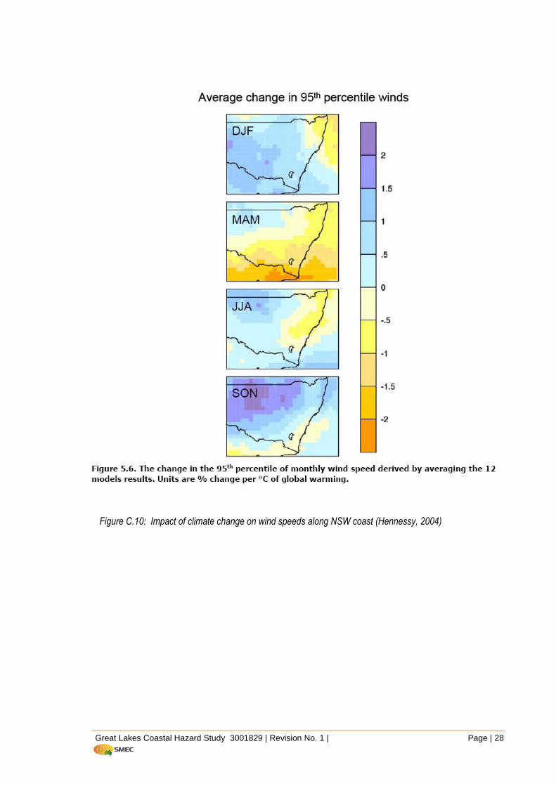
In addition to sea level rise, Climate change may cause changes in future storm frequencies and intensities, impacting on the severity of future beach erosion events. The potential for changes in storm intensity as a result of climate change has been considered below, by referring to modelling studies about future wind speeds under climate change (Hennessy et al., 2004).

Hennessy et. al. (2004) predicts no increase in winter storm wind speeds for the NSW coast as a result of climate change. Mean wind-speed projections show a tendency for increases across much of the state in summer, with decreases in the north-east. In autumn, there is a tendency toward weaker winds in the south and east, and stronger winds in the north-west. The tendency in winter is toward increases in the far north-west and south and decreases elsewhere. A tendency for stronger winds is evident in spring, with greatest increases across central NSW.

Projected changes in extreme monthly winds (strongest 5%) showed similar patterns to the mean wind changes in summer and autumn, except that the magnitude of the increases and decreases tended to be larger. In winter, changes in extreme winds differed from changes in mean winds in that most of the state and the ocean in the far south showed a tendency for increasing extreme winds with, only the north-east indicating decreasing winds. However, as shown in Figure C.10, for the north coast the tendency was for little change or decrease in extreme wind speeds. In spring, extreme winds tended to increase, in agreement with the mean wind speed changes, except in a small area on the southern half of the coast where there was a tendency towards decreasing extreme winds.

In the winter half-year, the modelling has indicated that Tasman Lows contributing to extreme winds increased in frequency from 26% at present to 31% by 2070. Frontal systems also increased from 25% of extreme wind days at present to 29% by 2070.


5 SUMMARY AND CONCLUSIONS

Climate change has the potential to affect the beaches at Great Lakes in two ways:

erosion/recession resulting from beach rotation, longshore drift and lake entrance behaviour at decadal time scales; and

overall beach recession resulting from sea level rise.

It was found that beach rotation, which is related to the Southern Oscillation Index, may result in decadal fluctuations in the beach berm of up to ±50 m on the more exposed longer beaches such as Bennetts or Nine Mile beaches with much less beach rotation at the shorter and more sheltered beaches. However, beach rotation would be limited by the presence of rock outcrops along the beaches.

The lake entrance dynamics and local sediment budget would also be impacted by changes to the mean wave climate brought about by climate change. A change in the frequency of El-Niño and La-Niña events would change the mean offshore wave direction and thus influence longshore sediment transport. A change toward dominant El-Niño conditions would lead to a more southerly wave climate enhanced northward sediment transport and a clockwise beach rotation (with recession at the southern end of the coast).

The IPCC (2007) projections for sea level rise caused by climate change have been synthesised with tectonic changes relevant for the NSW coast. The predicted shoreline response due to sea level rise at Great Lakes has been examined using a Bruun analysis. Sea level rise may also increase the volume of the tidal prism of the Wallis Lake and Smiths Lake when this lake is open. Breakwaters on both sides of Wallis Lake entrance would reduce the sediment infill into the estuary, however, would enhance the scour depth at the bottom of the entrance due both to sea level rise and a continuing response to the construction of the entrance breakwalls in the 1960s, with the Wallis Lake estuary shifting toward an unstable scouring mode (refer entrance stability analysis in Appendix G). Future changes to the estuary entrance dynamics of Smiths Lake are also possible, leading to an increased potential for breakthrough of the entrance through the tombolo at Smiths Lake entrance.


REFERENCES

Booij, N., R.C. Ris & L.H. Holthuijsen (1999). “A third-generation wave model for coastal regions, Part I, Model description and validation”, J.Geoph. Research, 104, C4, 7649-7666.

Bruun, P.M. (1954). “Coast erosion and the development of beach profiles”, Technical Memorandum 44, US Army Beach Erosion Board, June 1954.

Bruun, P.M. (1962). “Sea-Level rise as a cause of shore erosion”, Jnl. Waterways, Harbour & Coastal Engg. Div., ASCE, Vol. 88, No. WW1, pp 117-130.

Bruun, P.M. (1983). “Review of conditions for uses of the Bruun Rule of erosion”, Jnl. Coastal Engg., Vol 7, No. 1, pp 77-89.

Church, J.A., And White, N.J., (2011) Sea-Level Rise from the Late 19th to the early 21

st Century,

Survey and Geophysics, 32(4),585-6-2.

Dean, R. G. (1987) “Coastal sediment processes: toward engineering solutions.” In Nicholas C. Kraus, editor, Coastal Sediments ’87, volume 1, pp 1 – 24, New Orleans, Louisiana, May 1987. ASCE. Proceedings of a Specialty Conference on Advances in Understanding of Coastal Sediment Processes.

Department of Environment and Climate Change NSW (2009). “NSW Sea Level Rise Policy Statement”

Department of Environment and Climate Change NSW (2009). “Scientific basis of the 2009 sea level rise benchmark, Technical Note”.

Department of Environment and Climate Change NSW (2010). “Coastal Risk Management Guide - Incorporating sea level rise benchmarks in coastal risk assessments”

Goodwin, I.D. (2005). “A mid-shelf, mean wave direction climatology for southeastern AUSTRALIA, and its relationship to the El-Niño – Southern Oscillation since 1878 A.D.”, Int. J. Climatol. 25.

Goodwin, I.D., Verdon, D., Cowell, P. (2007). “Wave climate change, coastline response and hazard prediction in New South Wales, Australia”, Proceedings, Greenhouse 2007 conference, October 2007.

Hallermeier, R. J. (1981) “A profile zonation for seasonal sand beaches from wave climate” Coastal Engg., Vol. 4, pp 253-277.

Hallermeier, R. J. (1983) “Sand Transport limits in coastal structure design”, Proc. Coastal Structures ’83, ASCE, pp 703-716.

Hennessy, K., K. McInnes, D. Abbs, R. Jones, J. Bathols, R. Suppiah, J. Ricketts, T. Rafter, D. Collins* and D. Jones* (2004). “Climate Change in New South Wales Part 2: Projected changes in climate extremes” Consultancy report for the New South Wales Greenhouse Office by Climate Impact Group, CSIRO Atmospheric Research and *National Climate Centre, Australian Government Bureau of Meteorology, November 2004

Holthuijsen, L.H., Booij, N., Ris, R.C., Haagsma, IJ.G., Kieftenburg, A.T.M.M, Kriezi, E.E. (2000) “SWAN Cycle III version 40.11 User Manual”, Delft University of Technology, October, 2000.

IPCC (2001). Third Assessment Report Climate Change 2001: The Scientific Basis Working Group 1 of the Intergovernmental Panel on Climate Change, Shanghai, January, 2001.

IPCC (2007). “Climate Change 2007 – The Physical Science Basis, Fourth Assessment Report of Working Group 1 of the Intergovernmental Panel on Climate Change”, Cambridge University Press, Cambridge, United Kingdom and New York, NY, USA. 2007.


Kulmar, M., D. Lord & B. Sanderson (2005), “Future Directions of Wave Data collection in New South Wales.

McInnes, K.L., Abbs, D.J., O’Farrell, S.P., Macadam, I., O’grady, J. and Ranasinghe, R. (2007), “Projected Changes in Climatological Forcing for Coastal Erosion in NSW”, a project undertaken for the Department of Environment and Climate Change NSW, CSIRO Marine and Atmospheric Research, Victoria.

Mitchell, W., Chittleborough, J., Ronai, B. and Lennon, G. (2001), 'Sea Level Rise in Australia and the Pacific', in Proceedings of the Pacific Islands Conference on Climate Change, Climate Variability and Sea Level Rise, Linking Science and Policy, eds. M. Grzechnik and J. Chittleborough, Flinders Press, South Australia.

National Committee on Coastal and Ocean Engineering (2004) “Guidelines for Responding to the Effects of Climate Change in Coastal and Ocean Engineering” Engineers Australia, 2004.

Nielsen, A.F. and Gordon, A. (2007). “Assessing Estuary Stability”, Proceedings NSW Coastal Conference, Yamba NSW November 2007.

Nielsen, A. F. and Adamantidis, C. A. (2003) “A Field Validation of the SWAN Wave Transformation Program” Proc. Coasts and Ports Australasian Conference 2003.

Nielsen, A.F., D.B.Lord & H.G. Poulos (1992). “Dune Stability Considerations for Building Foundations”, ", IEAust., Aust. Civ. Eng. Trans., Vol. CE 34, No. 2 pp 167-173.

Nielsen, A. F. (1994) “Subaqueous Beach Fluctuations on the Australian South-Eastern Seaboard”, in Australian Civil Engineering Transactions, Vol. CE36 No.1 January 1994, pp 57-67.

Petkovic, P. & Buchanan, C. (2002). “Australian bathymetry and topography grid. [Digital Dataset].” Canberra: Geoscience Australia. http://www.ga.gov.au/general/technotes/20011023_32.jsp (13/9/2002).

PWD (1985), “Boomerang Beach and Blueys Beach Coastal Engineering Advice”. Public Works Department Civil Engineering Division. Ranasinghe, R., R. McLoughlin, A. Short & G. Symonds (2004). “The Southern Oscillation Index, wave climate, and beach rotation”, Marine Geology 204, 273−287.

Ranasinghe, R., Watson, P., Lord, D., Hanslow, D., Cowell, P. (2007). “Sea Level Rise, Coastal Recession and the Bruun Rule”, Proceedings Coasts and Ports Australasian Conference 2007.

Short, A.D., A.C. Trembanis & I.L. Turner (2000). “Beach oscillation, rotation and the Southern Oscillation, Narrabeen Beach, Australia”, Proc. 27th ICCE, ASCE, Sydney, July, 2000, 2439−2452.

SMEC Australia (2003). “Town Beach Hazard Definition Study”, Report no. 31460-001 prepared by Adamantidis, C. and Nielsen, A., August 2004.

Swart, D. H. (1974), “Offshore Sediment Transport and Equilibrium Beach Profiles”, Delft Hydraulics Laboratory, Publn. No. 131.

US National Research Council (1987), “Responding to changes in sea level – Engineering implications”, National Academy Press, Washington D.C.

Walsh, K.J.E., Betts, H., Church, J., Pittock, A.B., McInnes, K.L., Jackett, D.R. & McDougall, T.J. (2004) “Using sea level rise projections for urban planning in Australia” Journal of Coastal Research, Volume 20 Issue 2.

Young, I.R. (1999). “Wind Generated Ocean Waves”, Eds. R. Bhattacharyya & M.E. McCormick, Ocean Engineering Series, Elsevier, Amsterdam, 288 p.


FIGURES

Figure C.1: Wave rotation caused by El-Niño or La-Niña mean states (after Goodwin et al. 2007)


Figure C2: Example of change in nearshore angle caused by change in offshore wave approach angle from 127°TN to 140°TN at Number One Beach


Figure C.3: Measured global mean sea level 1870 – 2002 (White and Church, 2010)


Figure C.4: IPCC (2001) Sea level rise estimates


Figure C.5: IPCC (2007) Global average sea level rise estimates


Figure C.6: Concept of shoreline recession due to sea level rise


Figure C.7: Result of the sediment size analysis

0

10

20

30

40

50

60

70

80

90

100

0.01 0.1 1 10

% p

assi

ng

Sediment Diameter (mm)

Elizabeth Beach

Boat Beach

Main Beach

Bennetts Beach

Seven Mile Beach

One Mile Beach


Figure C.8: Suggested relationship for shape factor A vs. grain size D

Figure C.9: Nearshore profile at Boat Beach vs. idealised equilibrium profile

-30

-25

-20

-15

-10

-5

0

5

10

15

0 200 400 600 800 1000 1200 1400 1600

Idealised

Equilibrium Profile

Existing

Beach Profile


Figure C.10: Impact of climate change on wind speeds along NSW coast (Hennessy, 2004)

great lakes coastal hazard study - midcoast council€¦ · great lakes coastal hazard study...

Documents