GRB Trigger and Localization Algorithms Applied to GLAST Data Challenge One

Jerry T. Bonnell and Jay P. Norris Laboratory for High Energy Astrophysics

NASA/Goddard Space Flight Center, Greenbelt, MD 20771

March 31, 2004

1

ABSTRACT We describe an approach to triggering and localizing gamma-ray bursts (GRBs) detected by the LAT in GLAST’s Data Challenge 1 (DC1). The triggering algorithm, designed to determine if a burst in progress is detectable by the LAT, is based on a likelihood probability formulation comparing reconstructed event directions and intervals within a sliding temporal window. Ultimately, a modified version is intended to be utilized in an on-board GRB trigger capability for the LAT. In six days of DC1 LAT data, the algorithm was demonstrated to be robust, detecting 17 GRBs with no false triggers at the adopted threshold. Here, the trigger algorithm was evaluated in a realizable real-time procedure, but the burst localizations (and burst durations) presented are based on post facto considerations of the data and would need to be further adapted for use in on-board processing. However, we demonstrate that the LAT burst localizations possible in DC1 are sufficiently precise to support follow-up observations with optical telescopes, a strategy which can lead to redshift determinations via detecting burst counterparts.

2

1. INTRODUCTION Our central purpose is to utilize the machinery of GLAST’s Data Challenge One (DC1) to work towards perfecting the design of on-board gamma-ray burst (GRB) trigger and localization algorithms. More accurate localizations will in all probability be computed on the ground where essentially unlimited resources are available – but with associated delays of the order of hours. However, it is the prompt GRB localizations computed on-board GLAST and issued in alerts to the community that may have the most value, if in fact sufficient accuracy can be realized for on-board track reconstruction in a GRB processing algorithm. The rapid, accurate localizations that may be obtained for relatively fluent bursts at LAT energies are important since GRB optical and infrared afterglows usually fade rapidly. The afterglows quickly become inaccessible for intermediate to small telescopes whose ~ 15-30 arc minute fields of view (FOVs) can accommodate the localization uncertainties expected for LAT GRB detections. Optical and infrared detections of the afterglow lead to redshift determinations from the afterglow itself or the host galaxy. In the era when Swift and GLAST overlap (note that their FOVs will not always coincide) and beyond, actual spectroscopic redshifts rather than pseudo redshifts obtained purely from gamma-ray properties (Norris 2004), will still be indispensable: The extension of pulse shape analysis from BATSE and Swift energies to LAT energies will refine gamma-ray indicators of luminosity and total energetics by further constraining the jet dynamics of prompt emission. Also, to make useful constraints concerning the predicted effects of quantum gravity on propagation of light as a function of energy (e.g., Amelino-Camelia et al. 1998) will require accurate knowledge of burst redshifts, since the incurred delays are expected to be linear with distance as well as with energy. Here we are concerned with refinement of GRB trigger and localization algorithms. The DC1 environment provides conditions which presently are considerably different than those to be encountered in flight, but DC1 conditions can still be rendered to a useful approximation for some purposes. Twenty-one bursts were created for embedding within the first day of DC1 by collaborator Nicola Omodei, and twenty bursts were created for the next five days by one of us (JTB), the two groups using different simulation algorithms to make their synthetic bursts. In both sets the brightest bursts simulated were comparable in brightness to the most intense bursts which will be detected by GLAST in one year. The simulated bright bursts were overabundant (making their detection a foregone conclusion), so that sufficient photons would be detected per burst to allow interesting spectral analysis. Some dim bursts were also simulated, near the LAT threshold, to actually challenge the trigger algorithms. Triggering on the dim bursts was somewhat of a challenge only because we utilized the LAT’s full-FOV photon rate of DC1 as a pseudo background, eliminating just those photons which had no reconstruction, i.e., those with null instrument coordinates (θ, φ) = (0,0). This resulted in an average full-FOV rate of ~ 12 Hz. The LAT event rate telemetered to the ground is now expected to be much higher, ~ 300 Hz. However, the eventual (dominantly particle) background that will be presented to a GRB trigger algorithm may benefit from additional filters to be applied to a GRB event buffer, enabling the trigger algorithm to run on data rates of order ~ 15-30 Hz. The construction of sufficiently benign filters and of higher fidelity tracks to be presented to the GRB trigger algorithm(s) will occupy us in the coming months.

3

In the next section we describe the simple unbinned spatial and temporal trigger algorithm and the trigger results for the six days of DC1. An unbinned approach provides close to optimal sensitivity, although refinements to our specific implementation are conceivable, as will shortly be appreciated. In section 3 we then describe the localization algorithm, generation of errors, and comparison with the Monte Carlo truth positions. We note that variants on these algorithms may be useful for on-board and/or ground processing.

2. UNBINNED GRB TRIGGER ALGORITHM The general approach is to make maximal use of the unbinned photon data coming into the GRB buffer to form probabilities from the temporal and spatial information. The only quantities of interest are then the time intervals between photons and the distances between their estimated positions. In a real sense, the energy information is effectively used (but implicitly) in the correct degree, since the higher energy photons cluster more tightly, contributing lower chance probabilities than do photons of lower energy. So no explicit energy weighting is used in our current approach. To bootstrap the trigger procedure, either temporal or spatial information must be provided to the procedure initially. Some kind of sliding temporal window better suits the transient GRB problem, since the details of the time profile are not known a priori. Moreover, the spatial signature of a point source, the point spread function (PSF) of the LAT, is essentially known, and this definitive model can be compared with the detected photons, as we describe below. We use a sliding window which admits a constant number of photons, Nrange, in a variable time interval, rather than a variable number of photons in a fixed time interval. Alternatives on this bootstrap step are possible – including simultaneous consideration of information from all three dimensions, 2-D space + 1-D time – as mentioned in the discussion. In actual flight, several simultaneous triggers may be running (as we have simulated in previous studies) with different values of Nrange; or Nrange might vary automatically, taking into account the variable background rate. For this study it was sufficient to run one trigger with Nrange set at 20 photons. A second variable defines the number of photons to move forward, Nmove, in each iteration of the trigger procedure. We used our typical setting Nmove = ¼ Nrange = 5 photons. As the sliding window moves forward in time, the ambient background rate is computed, one Nrange prior to the trigger interval being examined. In practice, the background could (and probably should) be computed of order 10-50 seconds prior to the candidate trigger interval. The subprocedure “Formlike” is called, passing the times and instrument coordinates (θ, φ) for each of the Nrange photons, and the background rate, R, of the preceding Nrange interval. Formlike computes the N×(N–1) distances on the sphere between the Nrange photons. Note that with a background rate equal to Nrange photons s-1 (= 20 Hz), the instrument would scan ≈ 360°/5400 s-1 = 0.07° s-1, a negligible distance for the purpose of triggering, so use of instrument coordinates in this particular prescription is acceptable. For each photon there are (N–1) distances. Now each of the Nrange photons is considered the potential nucleus of a spatial cluster. For each of the N clusters, the (N’–1) distances between the nucleus photon and the other photons are retained which are less than a specified containment radius, ρ. We set ρ = 17°. That

4

cluster with the smallest average distance for the retained photons is further considered. The remaining clusters are discarded. To summarize, the adjustable variables in this trigger procedure are Nrange, Nmove, ρ, and the offset interval between the background interval and the trigger interval under consideration. Their adjustment may be rendered automatic (varying with background), or several simultaneous triggers may be run with different settings for the variables. For the chosen cluster with the smallest average distance, the interval between adjacent photons, ∆t, is computed for the (N’–1) retained photons. The chance spatial and temporal probabilities for the cluster are then computed. Relative to the expectation of random positional occurrence on the sky, the spatial probability involves only the (N’–1) distances, di : P(di) = [1 – cos(di)] / 2 , (1) We use the total log probability summed over the cluster, SumLogPdist = Σ log10[ P(di) ] (2) Similarly, the chance probabilities for the (N’–1) ∆t’s can be expressed using the integral of the interval probability distribution, where X = R∆t : P(∆ti) = 1 – (1 + X) e–X , (3) SumLogP∆t = Σ log10[ P(∆ti) ] (4) To allow for direct comparison of probabilities for two windows with different values for Nrange, a second term should be added to eqs. (2) and (4), – log10[Nrange]. These terms were included in our computations. The total unbinned, joint spatial and temporal log probability for the chosen cluster is then JointLogP = SumLogPdist + SumLogP∆t (5) The process repeats just by moving forward Nmove photons, dropping the oldest Nmove photons, and recomputing JointLogP (JLP) at each step. We recorded the rates, SumLogPdist, SumLogP∆t, and JLP values at each step for display and inspection. Figure 1 illustrates the raw rates and the log probabilities for the first day’s worth of DC1 data, in which the twenty-one Day One synthetic GRBs were embedded. Several interesting aspects are evident. The rates, illustrated in the bottom panel on a logarithmic scale, clearly show the effect of orbital modulation as the Galactic Center moves in and out of the LAT FOV. The GRBs are nearly periodically spaced, ≈ 4000 s apart, and so can easily be discerned in the rates if the burst occurred in or near the FOV. Red inverted triangles indicate the ten obvious bursts; black inverted triangles indicate bursts that are not obviously present, and are presumably outside the FOV. The second panel shows the trend of SumLogP∆t with a threshold for the temporal part of the log probability set at -15, drawn only to indicate that no “noise triggers”

5

Fig. 1 – Rates and log probabilities from unbinned trigger algorithm, Day One of DC1.

6

exceed this partial threshold. Eight GRBs exceed this temporal threshold. Notice that the burst present in the raw rates at ~ 47000 seconds (fifth red triangle from left in the rates panel) is completely absent in the SumLogP∆t plot. Some photons were detected, but none reconstructed for this burst, presumably because its position fell sufficiently far outside the LAT FOV, hence there was no spatial cluster identified from which to form ∆t’s. The spatial probability trend is shown in the third panel, with its partial threshold set at -25. The top panel shows the joint log probability with the total threshold of -40. Eleven bursts, marked with red triangles, exceed this threshold in Day One. A few noise spikes attain -34. However, the false trigger rate cannot be inferred to be 10(–40+34) = 10–6 per day since the rates vary. But we did fix the threshold at -40 and then examined the remaining five days of data. The next section describes the algorithm which localizes the bursts in space and time.

3. LOCALIZATION ALGORITHM The objectives are to find, as nearly as possible given the finite background rate, the first and last photons for a given burst, and estimate a spatial localization with error. In what follows the times, energies, and celestial coordinates (α,δ) – the DC1 data variables of interest – were examined only for reconstructed photons (i.e., the effective average rate was ~ 12 Hz). We proceeded through the record of joint log probability (JLP) versus time, setting a tstart. upon encountering the first JLP which exceeded the -40 threshold, and a tend for the last JLP exceeding threshold within ∆tsearch = 150 seconds of tstart. (Thus, bursts longer than ∆tsearch would be divided into two separate examination intervals.) The DC1 data variables of interest were then extracted for the localization interval ∆T = [tstart – tpreb , tend + tpost], with tpreb = 10 s and tpost = 30 s. An approximation to deriving the burst interval [tstart , tend], is incurred by the simple, schematic nature of the trigger algorithm implemented for this work. The background rate used in the interval probability statistic is derived from the previous Nrange interval considered by the procedure and hence begins to march into the burst interval, being completely contained within the burst at most Nrange events after the trigger. As such, the temporal contribution (see equations 3 and 4) to the running JLP record is underestimated, which could result in a systematic underestimate of the burst duration. For each of the Nrange windows the (α,δ) of the nucleus photon for the tightest cluster (see §2 above) was previously recorded. The celestial positions of the nucleus photons falling within the ∆T for a burst were averaged and used as the first rough estimate of the burst position. Then those photons falling with ∆T and within 7° of the nucleus photon were selected to be passed to the localization procedure, which we now outline. The primary ingredient is the weight to be assigned to each photon that contributes to the localization. Higher energy photons get larger weights, according to the energy-dependent PSF. The relevant PSF for DC1 is for the full-up (ground-based) reconstruction, whereas a less than optimal reconstruction will most probably be realizable in the LAT flight software. For

7

expediency we used one PSF, embodying the geometric mean of the approximate response of the thick and thin radiator layers, expressing the expected 1-σ error in position for a given photon as ε1σ(E) = C { 10 [-0.95log(E) + 1.523) + 1.0] + 0.03 } (6) where the error is in radians, and C = (1. × 1.35)½ is the mean of the thick and thin zones' PSF coefficients. However, not all selected photons necessarily come from the burst. Consequently, one background high-energy photon near (but not at) the center of the GRB photons’ cluster can destroy the accuracy of the localization. We remedied this problem by reassigning the error for any photon whose distance, d, from the nucleus photon exceeded 2 ×ε1σ(E) to be this distance ε = ε1σ(E) , d < 2 ×ε1σ(E) (7) = d , d ≥ 2 ×ε1σ(E) . Thereby, the energy of a background photon becomes moot in its weight for nucleus distances > 2 σ. The weights are then W = 1/ε. The two-dimensional weighted variables per photon are Xi = Wi

2 α cos(δ), Yi = Wi2 δi (8)

Defining Wtot = Σ Wi

2 , we have (Bevington 1969, Chapter 5) <X> = Σ Xi / Wtot <Y> = Σ Yi / Wtot (9) and with Λ = [N/(N–1)]½ where N is the number of selected photons, εX = Λ {Σ [ ((Xi/ Wi

2 - <X>)Wi2) 2] / (Wtot)

2 }½ , εY = Λ {Σ [ ((Yi/ Wi

2 - <Y>)Wi2) 2] / (Wtot)

2 }½ . (10) The weighted cluster centroid is then (αcen, δcen) = (<X> cos(<Y>) , <Y>) (11) with the estimated radial error ερ = { [εX /cos(εY)]2 + εY

2 }½ . (12) The procedure is iterated twice more, reselecting a new cluster within ∆T and now within 7° of (αcen, δcen) in lieu of the old nucleus photon’s position. The localization results of the third and final iteration are compiled in Table 1 for the 17 events which exceeded the trigger threshold. All these events are real GRBs; no false triggers resulted. Also listed are the numbers of detected photons per burst greater than 10 MeV, 100 MeV, and 1 GeV. Localization plots for the 17 GRBs are illustrated in the Appendix.

8

To identify as closely as possible the first and last photons in a burst, the inclusion threshold for the Nrange windows was lowered to -25 within the ∆T interval constructed for the localization procedure. Photons falling within 7° of the final (αcen, δcen) were deemed to belong to the burst; the times of the first and last of these photons are listed in Table 1 as Tstart and Tstop, respectively.

TABLE 1. Times, Localizations, and Integral Counts

NGRB Tstart Tstop αest δest N>10MeV N>100MeV N>1GeV _______________________________________________________________________________________________________________

1 3000.0 3005.8 200.140 -32.419 82 57 14 2 7022.2 7023.0 92.415 -1.171 8 4 0 3 11044.2 11047.3 326.879 27.145 21 18 6 4 19063.1 19067.2 138.656 -34.334 32 27 8 5 23139.1 23140.5 18.784 26.982 13 9 0 6 27210.5 27214.2 258.564 -15.926 35 30 7 7 35236.6 35242.3 97.766 -16.051 23 21 6 8 43254.6 43259.6 146.020 34.731 107 97 7 9 71386.4 71398.3 224.957 -33.485 71 51 2 10 75437.4 75456.3 91.945 56.558 753 556 65 11 83510.2 83514.8 200.050 -32.492 50 41 11 12 176748.2 176860.1 128.780 64.310 1634 1521 135 13 215700.4 215740.7 251.612 27.821 514 224 24 14 220440.4 220444.0 134.391 -2.809 329 309 32 15 327096.0 327096.0 319.802 73.287 11 5 0 16 386280.7 386309.7 199.136 33.451 59 28 1 17 410280.2 410313.4 236.714 41.721 371 52 10 _______________________________________________________________________________________________________________

3.1 Comparison with Monte Carlo Truth: Spatial Coordinates

Definitive Galactic positions exist for the first five bursts which we detect from the Day One set of simulated GRBs. Detected burst 11 shares the exactly same position as burst 1. Assuming a 2000 ephemeris, the (l, b) coordinates are converted to (α, δ) in Table 2. The coordinates for the six bursts which we simulated and detected on Days 2–6, bursts 12-17, are also listed in Table 2. (For the list of all incident photons for our synthetic bursts, see the MCtruth file, “sixdays20GRBs.txt” at http://glast.phys.washington.edu/DC1/sources/ ). The remaining Day One bursts which we detected, bursts 6-10, had celestial coordinates randomly generated within Gleam but not recorded for inspection. However, in most cases we were able to compute accurate celestial coordinates for these bursts using the MCtruth instrument coordinates – which of course moved with the scanning mode – by interpolating the pointing history. The history was recorded every minute (“pointing_history.root” at ftp://ftp-glast.slac.stanford.edu/glast.u10/DC1-cd/RootFiles/McTruth/ ). We extracted the MCtruth instrument coordinates for the 656 detected photons from Day One, computed (α, δ), examined

9

TABLE 2. Definitive Monte Carlo Positions, Detected Bursts

NGRB l act bact αact δact ______________________________________________________________________

1 -50.000 30.000 200.116 -32.473 2 -150.000 -10.000 92.628 -1.968 3 80.000 -20.000 326.861 27.153 4 -100.000 10.000 138.634 -34.231 5 130.000 -35.000 18.784 26.982 11 -50.000 30.000 200.116 -32.473 12 151.542 35.405 128.738 64.291 13 48.217 38.333 251.690 27.830 14 231.102 26.247 134.306 -2.709 15 108.539 16.793 317.710 73.143 16 83.080 81.559 199.333 33.459 17 66.814 51.460 236.747 41.743 ______________________________________________________________________

TABLE 3. Comparison of Positions, Actual and Estimated

NGRB αact δact αest δest εest εact Nsigma __________________________________________________________________________________________________________

1 200.116 -32.473 200.140 -32.419 0.068 0.058 0.848 2 92.628 -1.968 92.415 -1.171 0.292 0.825 2.825 3 326.861 27.153 326.879 27.145 0.109 0.018 0.164 4 138.634 -34.231 138.656 -34.334 0.055 0.105 1.902 5 19.385 27.513 18.784 26.982 0.472 0.753 1.596 6 258.724 -15.818 258.564 -15.926 0.095 0.188 1.979 7 97.729 -15.954 97.766 -16.051 0.094 0.103 1.099 8 146.063 34.721 146.020 34.731 0.073 0.037 0.503 9 224.942 -33.562 224.957 -33.485 0.056 0.078 1.393 10 91.952 56.536 91.945 56.558 0.035 0.022 0.638 11 200.116 -32.473 200.050 -32.492 0.044 0.059 1.337 12 128.738 64.291 128.780 64.310 0.029 0.026 0.907 13 251.690 27.830 251.612 27.821 0.090 0.070 0.773 14 134.306 -2.709 134.391 -2.809 0.052 0.131 2.523 15 317.710 73.143 319.802 73.287 4.418 0.621 0.141 16 199.333 33.459 199.136 33.451 0.346 0.165 0.476 17 236.747 41.743 236.714 41.721 0.122 0.033 0.271 __________________________________________________________________________________________________________

10

the trends, and averaged the (αi, δi) per burst. The (αi, δi) trends often did not vary by more than 2–3 thousands of a degree in each coordinate. However, bursts 1, 6, 10, and 11 varied by a few hundredths. Burst 4 was the most egregious, being consistently off from the MCtruth by ~ 1° in the αi. Thus our estimated errors can be compared to a precision of ~ 0.03° – 0.003° with the actual errors. Table 3 summarizes the true and estimated positions, estimated and actual errors, and the ratio, εest/εact, called “Nsigma”. By examining the pointing history closely, we determined that the MCtruth instrument coordinates for the X and Z axes shifted abruptly right after the commencement of burst 6, which shift we came to understand was an “instantaneous” rocking maneuver (T. Burnett, private communication). Thus we quote only the first computation of (α, δ) for burst 6 in Table 3. We presume that similar maneuvers (or interpolation within the coarse 1-minute pointing history grid) probably gave rise to the variations of order a few hundredths of a degree discussed above. Fig. 2 – “Nsigma” (= estimated error radius / actual error radius) versus number of ID’ed photons with measured energy > 100 MeV. See Tables 1 and 2 for numerical values. Our estimated errors are usually in reasonable agreement with the actual errors, as evidenced by the fact that their ratio, Nsigma, is of order unity. Figure 2 shows a scatter plot of Nsigma versus number of detected photons with energy > 100 MeV. There does not appears to be any

11

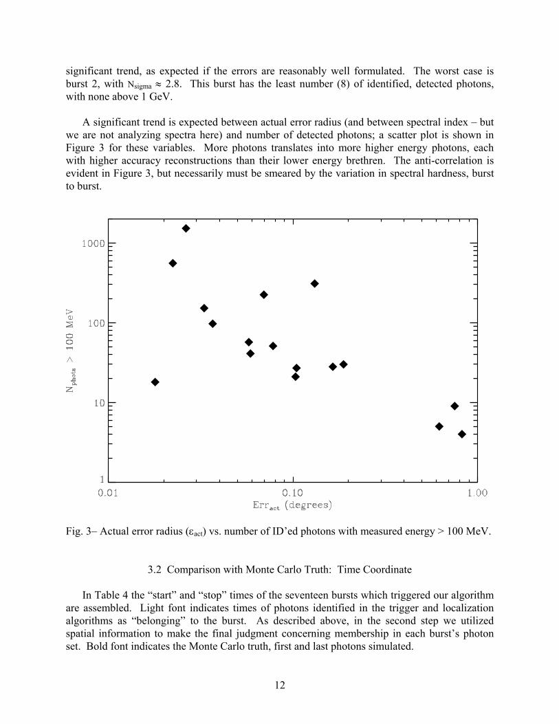
significant trend, as expected if the errors are reasonably well formulated. The worst case is burst 2, with Nsigma ≈ 2.8. This burst has the least number (8) of identified, detected photons, with none above 1 GeV. A significant trend is expected between actual error radius (and between spectral index – but we are not analyzing spectra here) and number of detected photons; a scatter plot is shown in Figure 3 for these variables. More photons translates into more higher energy photons, each with higher accuracy reconstructions than their lower energy brethren. The anti-correlation is evident in Figure 3, but necessarily must be smeared by the variation in spectral hardness, burst to burst. Fig. 3– Actual error radius (εact) vs. number of ID’ed photons with measured energy > 100 MeV.

3.2 Comparison with Monte Carlo Truth: Time Coordinate In Table 4 the “start” and “stop” times of the seventeen bursts which triggered our algorithm are assembled. Light font indicates times of photons identified in the trigger and localization algorithms as “belonging” to the burst. As described above, in the second step we utilized spatial information to make the final judgment concerning membership in each burst’s photon set. Bold font indicates the Monte Carlo truth, first and last photons simulated.

12

TABLE 4. Comparison of Initial and Final Times, Actual and Estimated

NGRB Tstart Tstop _______________________________________________

1 3000.0 3005.8 3000.04 3009.38 2 7022.2 7023.0 7022.19 7032.76 3 11044.2 11047.3 11044.30 11054.00 4 19063.1 19067.2 19063.10 19067.20 5 23139.1 23140.5 23136.30 23140.10 6 27210.5 27214.2 27209.70 27221.30 7 35236.6 35242.3 35235.90 35241.20 8 43254.6 43259.6 43254.60 43262.10 9 71386.4 71398.3 71386.20 71404.80 10 75437.4 75456.3 75437.50 75464.60 11 83510.2 83514.8 83510.20 83516.40 12 176748.2 176860.1 176748.13 176860.12 13 215700.4 215740.7 215700.45 215740.77 14 220440.4 220444.0 220440.37 220444.11 15 327096.0 327096.0 327096.00 327096.01 16 386280.7 386309.7 386280.73 386324.52 17 410280.2 410313.4 410280.10 410315.11 _______________________________________________

Light: Burst ID’ed first and last photon times. Bold: Actual first and last photon times. Black and Red fonts – see text. In addition there is an “apples and oranges” flavor to Table 4 attributable to the totality of the available information, which differs for the two approaches used to simulate bursts. For the Day One bursts (black font) we quote the Monte Carlo times of detected photons. However, the

13

photon list for our bursts was grown using IDL procedures, then submitted to Gleam for detection. Our list (sixdays20GRBs.txt, discussed above; red font) includes all the incident photons which illuminate the 6 m2 sphere surrounding the LAT instrument; only a small fraction (~10–15%) of these photons impinge on the detectors. Consider the start times for all seventeen bursts. In fourteen cases, the agreement between times of first identified photon and first Monte Carlo photon is ~ 0.1 s; the largest offset is ~ 3 s. Also, for five of six of our bursts (red font) last photon times agree to within two seconds. However, for the Day One bursts, the difference between truth and detected last photons is usually at least a few seconds and ranges up to ~ 8 s. This generally larger discrepancy may be attributable to three effects: The pulses in the Day One bursts may decay more slowly (we do not have any information to suggest that this is actually the case). Also, we understand that the mechanism for stopping a burst that is manufactured within Gleam using the GRBsim module entails a rate time generator that may produce at least one photon distanced from the main, intended emission. Finally, as discussed in section 3, the JLP determination tends to overestimate the background rate after the burst has been detected and therefore tends to produce underestimates of the burst duration. Hence, we are not at all certain of the last photon times for bursts 1 through 11. Note that for burst 7 we find the last photon to be ~ 1.1 s after the last Monte Carlo photon; thus this photon cannot belong to the burst.

4. SUMMARY AND DISCUSSION We have used simulated LAT data from DC1 to test one realization of a simple unbinned algorithm for triggering on and localizing GRBs. The algorithm computes a running joint log probability (JLP) likelihood function for the data record, combining spatial and temporal information in a fixed Nevent = 20 sliding window. The algorithm is applied to the total DC1 simulated event rate, after eliminating only the spatially unreconstructed events from consideration, thereby yielding an average rate of about 12 Hz. Within the six days of DC1 LAT data, the algorithm was demonstrated to be robust, detecting 17 GRBs with no false triggers at the adopted JLP threshold of -40. An inspection of noise spikes in the running JLP computation indicates that this threshold is consistent with a formal expectation of 10-6 false triggers per day, but only if a constant background rate is assumed, and only if the noise distribution were in fact Poisson distributed (this never happens in reality). Still, this threshold for triggering on bursts is clearly insensitive to variations in the DC1 cosmic background introduced by the Galactic Center transiting the LAT FOV. Burst durations were determined to within a few seconds. Localization errors based on knowledge of the Monte Carlo source positions are demonstrated to be better than 0.1 degrees in some cases. In all cases where Monte Carlo source positions were available, the measured positions are consistent with the derived statistical errors. While Monte Carlo positions are available for reconstructed events in instrument coordinates, the comparison of true positions vs. measured ones for cosmic sources could be easily facilitated by including a Monte Carlo truth sky coordinate pair for each simulated LAT photon.

14

We emphasize that the localization errors demonstrated here are commensurate with FOVs of optical telescopes capable of timely detections of burst counterparts. This indicates that the LAT itself could support rapid follow-up observations ultimately resulting in redshift determinations for the bursters. We consider this to be the major motivation for developing an on-board triggering capability for the LAT. However, we recognize that the relevant PSF for DC1 is for the full-up (ground-based) reconstruction, whereas a less than optimal reconstruction will most probably be realizable in the LAT flight software. Also, the bursts generated for DC1 by both groups tended toward the bright end of the peak flux distribution, and so they are better localized than will be the majority of real bursts to be detected by the LAT, which will be dim. The on-board background rate seen by the LAT GRB trigger algorithm will likely be worse than the ~ 12 Hz event data, considered as an effective background in this exercise of the GRB triggering algorithm, but maybe not much worse: The background coming into to a GRB event buffer to be presented to the trigger algorithm may benefit from additional on-board filters, yet to be constructed. The construction of sufficiently benign filters and of higher fidelity tracks to be presented to the GRB trigger algorithm(s) will occupy us in the coming months. In successfully searching for DC1 GRB triggers we use a sliding window which admits a constant number of photons, Nrange, in a variable time interval, rather than a variable number of photons in a fixed time interval. Prior to DC1, our extensive LAT GRB trigger simulations have explored background rates of up to 64 Hz and indicate that it will be advantageous to consider simultaneously multiple sliding windows differing in Nrange (e.g. 20, 40, 80 event windows). Alternatively, admitting a variable number of photons within a fixed time in the running JLP estimation may also be effective against variable backgrounds. However, we are encouraged that adopting a single, fixed 20-event sliding window (the smallest window we have ever considered), easily detected bursts against the effective background simulated in DC1. A possible alternative to our temporal bootstrap approach for the trigger is to consider information from all three dimensions (2-D space + 1-D time) simultaneously. An n-dimensional Bayesian Block formulation is described in Scargle et al. (2004) that might be suitably adapted to our GRB trigger problem. REFERENCES Amelino-Camelia, G. et al. 1998, Nature, 393, 319 Bevington, P.R. 1969, “Data Reduction and Error Analysis for the Physical Sciences”

(McGraw-Hill: New York), Chapter 5 Norris, J.P. 2004, Baltic Astronomy, vol 12, Proc. of JENAM Conference, Budapest, in press,

astro-ph/0312279 Scargle, J.D., et al. 2004, in preparation

15

APPENDIX: LOCALIZATION PLOTS The 17 events which triggered our algorithm – all confirmed to be amongst the simulated GRBs – are plotted here in celestial coordinates. The plots are equal scale in the two coordinates, and the estimated centroid position (Table 1) is coincident with the plot center. Photons within 7° of the centroid and judged by the localization algorithm to be “associated” with the burst are plotted as circles. Color coding indicates one of three energy ranges (measured photon energy): Black: 10 MeV < E < 100 MeV Blue: 100 MeV < E < 1000 GeV Red: 1000 MeV < E The red circle, usually visible, has a diameter 10 times that of the estimated error circle. Notice that the red colored, high energy photons usually fall inside the plotted circle. One perceives the qualitative impression that the high energy photons by themselves determine the estimated GRB position. However, we have experimented by excluding the (lower weighted) lower energy photons and have found that in fact they contribute their share (eq. [6]) to enhancing the accuracy of the localization. The (small) red circles are barely discernible in bursts # 10 and 12, masked by the many high energy photons. The red circle is outside the plot bounds for burst # 15 since 10 times the estimated error radius is more than 40°.

16

17

18

Note: The red circle, usually visible, has a diameter 10 times that of the estimated error circle.

19

20