gray whale (eschrichtius robustus) abundance during … · la ruta migratoria anual de esta ballena...
TRANSCRIPT
CENTRO DE INVESTIGACIÓN CIENTÍFICA Y DE EDUCACIÓN SUPERIOR
DE ENSENADA
PROGRAMA DE POSGRADO EN CIENCIAS
EN ECOLOGÍA MARINA
GRAY WHALE (Eschrichtius robustus) ABUNDANCE DURING ITS
MIGRATION IN ENSENADA, BAJA CALIFORNIA, DURING THREE
SEASONS (2003-2006)
TESIS
que para cubrir parcialmente los requisitos necesarios para obtener el grado de MAESTRO EN CIENCIAS
Presenta:
MELBA DE JESUS HUERTA
Ensenada, Baja California, México, Octubre 2007.
ii
RESUMEN de la tesis que presenta Melba De Jesús Huerta, como requisito parcial para la obtención del grado de MAESTRO EN CIENCIAS en ECOLOGIA MARINA, Ensenada, Baja California, octubre 2007. Resumen aprobado por: ___________________________
Dra. Gisela Heckel Dziendzielewski Abundancia de ballena gris (Eschrichtius robustus) durante su migración en Ensenada, Baja California, en tres temporadas (2003-2006). Actualmente sólo existen dos poblaciones de ballena gris que han pasado por momentos en donde se les consideró casi extintas. La población del Pacífico Occidental, que se encuentra a lo largo de las costas asiáticas, aún se considera en peligro de extinción. La población del Pacífico oriental se ha recuperado y ha sido monitoreada desde los años cincuenta. Este estudio se enfoca en esta población. La ruta migratoria anual de esta ballena es a lo largo de las costas de Norteamérica, desde los mares de Chuckchi y Beaufort hasta las lagunas costeras de Baja California Sur, México. Su extensa ruta migratoria hace de la ballena gris un recurso compartido entre tres naciones, y por lo tanto, la contribución para su conservación debe ser una responsabilidad de todas ellas. Los conteos de ballena gris durante su migración no se habían realizado en México antes del presente estudio. Nuestros objetivos fueron determinar los tiempos de la migración (inicio, máximo, fin) al sur y al norte, y estimar el tamaño poblacional con base en las ballenas contadas en la migración al sur. Se llevaron a cabo censos durante tres años (diciembre a mayo 2003-2006) desde la costa en Ensenada, Baja California, México. Los tiempos de la migración se determinaron para las migraciones al sur y al norte por medio de un índice de abundancia relativa (número de ballenas por hora de esfuerzo de observación). Para la estimación de abundancia se tomaron en cuenta factores que podrían sesgar la estimación final: ballenas no observadas durante horas de esfuerzo, corrección por tamaño de grupo y por sesgo del observador, ballenas no observadas durante periodos sin esfuerzo ( tf ) por medio de polinomiales de Hermite, distancia de la costa (por medio de recorridos en barco) y variación de la tasa migratoria entre el día y la noche. Los conteos promedio fueron de 3.97, 3.87 y 3.56 ballenas/hr en 2003-2004, 2004-2005 y 2005-2006, respectivamente. Los tiempos de migración fueron consistentes en 2003-04 y 2005-06, y se presentaron fechas medianas del 23 al 29 de enero. Las fechas medianas para 2004-05 fueron una semana más temprano, entre el 17 y el 18 de enero. Para los tres años, la consistencia permaneció para la fecha en la cual se registró el 90% de los avistamientos (13 de febrero). La migración al norte mostró una serie de tiempo más prolongada, y se dividió en migración al norte sin crías y migración sólo de parejas hembra/cría. La migración al norte sin crías ocurrió desde mediados de febrero hasta principios de abril con conteos de 1.03, 1.50 y 0.52 ballenas/hr en los respectivos años de 2003 a 2006. El segundo grupo de migrantes (parejas hembra/cría) pasaron por Ensenada desde principios de abril hasta principios de mayo con conteos menores (0.43, 0.19 y 0.26 parejas hembra/cría por año). El traslapo entre los dos periodos de migración al norte fue a principios de abril. Se contaron un total de 661, 773 y
iii
661 ballenas durante la migración al sur en 2003-04, 2004-05 y 2005-06, respectivamente, Los recorridos en barco mostraron que 56% de los avistamientos de ballenas grises que pasan por Ensenada no pueden ser observadas desde tierra porque pasan a más de 5km de la costa; por lo tanto, se aplicó un factor multiplicativo general de 1.56. Se obtuvieron valores altos de tf : 12.46 (2003-04), 12.96 (2004-05) y 9.77 (2005-06)). La estimación final de la abundancia de ballena gris en Ensenada fue de 24,862 individuos en 2003-04, 29,786 en 2004-05 y 19,436 ballenas en 2005-06. Palabras clave: Ballena gris, Eschrichtius robustus, abundancia, estimación, migración, factores de corrección.
iv
ABSTRACT of the thesis presented by Melba De Jesús Huerta, as a partial requirement to obtain the degree in MASTER OF SCIENCE in MARINE ECOLOGY, Ensenada, Baja, California, Mexico, October 2006. Abstract approved by: ____________________________
Gisela Heckel Dziendzielewski, Ph.D. Gray whale (Eschrichtius robustus) abundance during its migration in Ensenada, Baja California, during three seasons (2003-2006). In present time, there are only two extant gray whale populations that have gone through critical points of near extinction. The Western Pacific stock, found along eastern Asian coasts, still remains endangered. The Eastern stock has recovered and has been monitored systematically since the 1950’s. The present study is focused on this population. This whale’s annual migration route is along the North American coasts, from the Chukchi and Beaufort seas to coastal lagoons in Baja California Sur, Mexico. Its extended migration route makes gray whales a common resource shared among three nations. Therefore, contribution for its conservation should be a three-nation responsibility. Gray whale counts during its migration in Mexico had not been attempted prior to this study. Our objectives were to determine the south- and northbound migration timing (beginning, peak, end) and to estimate the population size based on southbound migrating whale counts. We carried out onshore censuses during three years (December to May 2003-2006) in Ensenada, Baja California, Mexico. Migration timing was determined for southbound and northbound migration periods with a relative abundance index (number of whales per hour of observation effort). Abundance estimation took into account factors that may bias the final estimation: whales missed during effort periods, bias corrected pod size and observer bias, whales missed during off-effort periods ( tf ) with Hermite polynomials, distance offshore (by means of boat surveys), and day/night travel rate. Mean counts varied from 3.97, 3.87, to 3.56 whales/hr in 2003-2004, 2004-2005, and 2005-2006, respectively. Migration timing was consistent in 2003-04 and 2005-06, with median dates ranging from 23-29 January. Median dates for 2004-05 were about a week earlier on 17-18 January. For all three years, consistency prevailed in the observed date (13 February) on which 90% of the southbound sightings were recorded. The northbound migration showed a more prolonged time series, splitting it into northbound migration without calves and migration with only cow/calf pairs. Northbound migration without calves lasted from mid-February to early April with mean counts of 1.03, 1.50, and 0.52 whales/hr in the respective years from 2003-2006. The second set of migrants (cow/calf pairs) traveled past Ensenada from early April to early May with lower mean counts of 0.43, 0.19, and 0.26 cow/calf pairs day-1 per year. The overlap in the two northbound migration groups was in early April. A total of 661, 773, and
v
661 whales were counted in 2003-04, 2004-05 and 2005-06, respectively, for the southbound migration. Boat surveys revealed that 56% of gray whale sightings cannot be observed from land because the whales are traveling beyond 5km from shore; therefore, a correction factor of 1.56 was calculated as a general multiplicative factor. High tf values were obtained: 12.46 (2003-04), 12.96 (2004-05), 9.77 (2005-06). Final estimated gray whale abundance in Ensenada was 24,862 whales in 2003-04, 29,786 whales in 2004-05 and 19,436 whales in 2005-06.
Key words: Gray whale, Eschrichtius robustus, abundance, estimation, migration, correction factors.

vi
IN SPECIAL DEDICATION TO:
Adriana and Pablo (This is your harvest)
My grandma
Norma
Angel (It was hard to work with your absence)
Sarah and the little one…
Ari---Vivi---Ixchel
vii
ACKNOWLEDGEMENTS First of all, I thank CICESE for being the source of the completion of my degree in accepting me in its Marine Ecology grad program and for sponsoring my last trimester at the institution (PEM scholarship). Also, I am in gratitude to the Consejo Nacional de Ciencia y Tecnología (CONACYT) for financing most of my stay at CICESE. Shell Mexico, S.A. de C.V. and Energía Costa Azul, S. de R.L. de C.V. made this research possible by financing the project. Special thanks to Dr. Gisela Heckel for accepting to be my advisor, even after she had more grad students than she could ask for. Thank your tutoring, your advices, for listening to me as a friend but most of all thank you for letting me enter and taste marine mammal research. I loved it! My gratitude to Dr. Oscar Sosa, Dr. Victor Ruiz and Dr. Stephen B. Reilly, for taking part as my committee members. Dr. Stephen B. Reilly not only took me in as his student but he also guided and gave me good advices throughout my thesis progress. I can never be too grateful to Dr. Jeffrey Breiwick for his patience, tutoring and advices he unconditionally gave me without knowing me. I hope I can someday thank you in person. These analyses could not have been done without long, exhaustive, but fun hours of field work. Alejandra Baez, Guadalupe Gómez, Luis Enríquez, Denise Lubinsky, Nelva Victoria, Ligeia del Toro, Nemer Narchi, Erick Bravo, Laura Barboza, Concepción García, Ivonne Posada, Aileen Gaset, Esther Araiza, Jorge López, Héctor Pérez and Gemma Rivera all worked hard and helped in gathering the “raw data.” MY FAMILY. I am in eternal gratitude to my parents (PABLO and ADRIANA) for opening my career paths. Thank you to my brother (Angel) and sisters (Norma and Sarah) for always being there regardless of distance. My grandmother with her speeches. My little rascal nieces Ari, Vivi and Ixchel who rushed me. Can’t forget my faithful companion, Galette ☺, in the long nights of work at CICESE. You are all the main reason why I am still standing and still running forward!!! Can’t forget my friends and helping hands!!!!! Thank you Gemma for cheering me on and for your guidance; you go beyond friendship. Adriana with your advices, Jacobo (new learnings), Hector (two heads are better than one), Carix, Erica, Aleix (thank you for your guidance with the R Program), Ale (your help & patience), Esther…….. and the list goes on……

viii
RESUMEN EJECUTIVO
I. INTRODUCCIÓN
La larga ruta migratoria de la población del Pacífico nororiental de la ballena gris
(Eschrichtius robustus; Lilljeborg, 1861), hace de este misticeto un recurso compartido por
tres naciones: Canadá, Estados Unidos y México. Independientemente del acuerdo que
exista entre las naciones para manejar un recurso, el principio básico para manejarlo es el
conocer la salud y estado del mismo así como también del ambiente que lo rodea. La
migración anual y costera de la ballena gris, que es la más larga de los mamíferos, resulta
conveniente para el constante monitoreo de esta especie permitiendo conteos anuales desde
tierra. Con base en los conteos es posible estimar el tamaño de esta población. Sin embargo,
las estimaciones pueden estar sesgadas por factores que puedan afectar los conteos. Aunque
se han realizado estimaciones en California (Granite Canyon) casi cada año desde la década
de los sesenta, desde 2002-2003 esta información no se registró. En el presente estudio se
estimó el tamaño de la población de ballena gris del Pacifico Nororiental en tres
temporadas (2003-04, 2004-05, 2005-06), tomando en cuenta los factores que sesgan la
estimación final. En México, este método de estimación de abundancia no se había
aplicado. El estudio se podría tomar como un indicador de participación por parte de
México en el monitoreo de un recurso que también le pertenece.
Caza de la ballena gris del Pacifico nororiental
A mediados del siglo XIX, una de las especies de ballenas más afectadas por la caza fue la
ballena gris. Existían tres poblaciones de ballena gris distribuidas alrededor del hemisferio

ix
norte antes de que iniciara la caza: en el Atlántico, el Pacifico nororiental y el Pacífico
noroccidental. La caza intensa posiblemente fue de los mayores contribuyentes en la
extinción del stock del Atlántico (Bryant, 1995), y actualmente sólo existen los dos stocks
del Océano Pacífico (Rice and Wolman, 1971). Éstos han pasado por un punto de
agotamiento. La caza incontrolada fue probablemente la causa principal en agotar el stock
del Pacifico noroccidental, al grado de que se había llegado a dudar de su existencia (Mizue
1951; Bowen, 1974). Aun existente, este stock se encuentra en peligro de extinción
(Brownell and Chun, 1977; Blokhin, et al., 1985). De los tres stocks que pasaron por
niveles de agotamiento, el único en recuperarse ha sido el de la ballena gris del Pacifico
oriental. Su caza comercial inició en 1846 y sólo se extendió hasta 1874 debido a una
intensa caza no controlada. En 1937, se dio protección a esta especie en Estados Unidos,
donde se incluyó en la lista de especies en peligro de extinción (U.S. Endangered and
Threatened Wild Life List, Federal Rule 59 FR 31095; MBC Applied Environmental
Science, 1989; COSEWIC, 2004). En México se ha considerado como una especie
protegida desde 1994, además de que sus lagunas de reproducción se han protegido desde
1972 (SEMARNAT, 2002). Hoy en día, esta población se ha recuperado y se ha ubicado en
la categoría de “baja preocupación” de la Lista Roja de la Unión para la Conservación de la
Naturaleza y Recursos Naturales (IUCN por sus siglas en inglés; Cetacean Specialist Group
1996).
Información general e importancia de la población del Pacifico Nororiental
La ballena gris (Eschrichtius robustus) es la única especie representativa de la familia
Eschrichtiidae. No presenta una aleta dorsal, y en su lugar tiene una pequeña “joroba”,

x
seguida de 6 a 14 protuberancias. La longitud de la ballena gris es de aproximadamente 4.6-
4.9m al nacer y en promedio de 14m en la etapa adulta; donde las hembras son de mayor
tamaño que los machos (Jones and Swartz, 2002; Reeves et al., 2002). Como todas las
ballenas, esta especie es longeva y alcanza la madurez sexual a los ocho años. Su
reproducción es bienal y se caracteriza por migrar grandes distancias para llevarla a cabo.
Anualmente, la ballena gris migra entre 8,000 y 10,000 km. (Rugh et al., 2001) desde su
zona de alimentación (mares de Bering y Chuckchi) a las lagunas de reproducción en Baja
California, México. Se le considera una especie clave en el ecosistema Bering-Chuckchi.
Ecológicamente, esta especie toma importancia en eventos sucesivos bentónicos debido a
sus hábitos alimenticios, ya que aspira el sedimento del fondo marino, donde viven sus
presas preferidas, los anfípodos bentónicos. Su importancia se extiende más allá de lo
ecológico, puesto que también se le atribuyen valores económicos y culturales. En lo que a
lo económico se refiere, los ingresos monetarios provienen de avistamientos turísticos de
ballena gris a lo largo de su ruta migratoria. La importancia cultural prevalece en las zonas
de alimentación, donde la cazan aborígenes con con fines de subsistencia.
Antecedentes
Antes de los métodos que actualmente se conocen, la única forma de conocer la población
de ballenas era por medio de registros de captura por unidad de esfuerzo, es decir, por
registros de caza (Allen, 1980). Con el tiempo, los métodos evolucionaron y hoy en día se
puede estimar el tamaño de la población mediante conteos desde tierra. La metodología se
ha vuelto meticulosa y se han contemplado factores que puedan sesgar la estimación del
tamaño de la población. Se han hecho modificaciones detalladas de estas correcciones para

xi
precisar la estimación final a un número cercano a la realidad. En su mayoría, estos
estudios se han realizado en Granite Canyon, California. Reilly et al. (1983) realizaron un
estudio de una serie de tiempo de 13 años, y estimaron el tamaño de la población para cada
temporada. Estos autores iniciaron el cálculo de factores para corregir errores o sesgos en la
estimación, tales como ballenas no observadas durante horas sin esfuerzo, sesgo en la
estimación del tamaño de grupo por variaciones entre los observadores, así como por
factores ambientales y variación en la tasa de nado entre el día y la noche. Este último
factor no pudo ser corregido por estos autores debido a un sesgo en la hora inicial de
esfuerzo. La corrección fue determinada por Perryman et al, (1999) quienes mediante el
uso de sensores de imágenes térmicas, determinaron un factor de corrección en la variación
de la tasa nado en la noche de 1.0875 ( *nf = 1.0875).
El sesgo en detectar un grupo de ballenas y determinar su tamaño también se ha
contemplado desde los estudios de Reilly et al. (1980). Además, Rugh et al. (1990),
condujeron un experimento con observaciones pareadas determinar el número de ballenas
que no se observan durante horas de esfuerzo (probabilidad de detección). Este estudio fue
detallado en 1993 por Rugh et al., extendiendo el tiempo del experimento y desarrollando
un algoritmo de puntaje para determinar la probabilidad de detectar la ballena.
Un factor que puede resultar de gran importancia si el corredor migratorio es amplio es el
número de ballenas no observadas debido a que pasan a una distancia a la costa tan amplia
que no es posible detectarlas. Shelden y Laake (2002) realizaron un estudio mediante
censos aéreos en Granite Canyon, California, y determinaron que no era necesario corregir
este factor, puesto que más del 90% de la población pasaba a la vista del observador, a
xii
menos de 5.6km de la costa. Sin embargo, en sitios como Washington esto no sucede.
Green et al. (2005) determinaron que el ancho del corredor migratorio se extiende ahí a 40
km de la costa.
El tamaño de la población se subestima si el número de ballenas que pasan fuera de horas
de esfuerzo no se toma en cuenta. Para esto, se han desarrollado métodos menos complejos
que el uso de la distribución Gamma. Buckland (1992) diseñó un algoritmo utilizando
polinomios de Hermite para interpolar sobre la distribución de los avistamientos obtenidos
y así contemplar el número de ballenas no observadas durante periodos fuera de esfuerzo.
Importancia del trabajo
Se sabe que las poblaciones no son constantes y esto se evidencia en las fluctuaciones de la
población de ballena gris del Pacífico nororiental, a lo largo de los años que se han
estudiado. En las temporadas que se contemplaron en este estudio desde el 2003 al 2006, no
se conocen registros de conteos o estimaciones del tamaño de la población. Las últimas
estimaciones se realizaron en el 2002 y, según Rugh et al. (2005), la población disminuyó
desde el 2001. El presente trabajo puede contribuir al conocimiento de la abundancia de la
población en los años en los cuales no se registró alguna estimación. Aunado a esto, en
México esta información es casi nula, por lo tanto este estudio puede proporcionar una
contribución preliminar de estimación de abundancia de ballena gris.
xiii
HIPÓTESIS
La población de ballena gris del Pacífico nororiental ha pasado por cambios importantes.
Springer (2002) resalta un posible decremento de 30% en el ecosistema de Bering-
Chuckchi en los últimos 30 años. Por lo tanto, esta población pudo haber disminuido desde
el 2002, el último año en que se registró una estimación en California.
OBJETIVOS
Objetivo General
Con el fin de generar nueva información en México y en la serie de tiempo anual sobre la
abundancia de la ballena gris, este estudio estimó la abundancia de ballena gris del Pacífico
nororiental durante su migración al sur en tres temporadas (diciembre a mayo 2003-2004,
2004-2005, y 2005-2006).
Objetivos específicos
• Determinar el tiempo de la migración al sur y al norte (inicio, máximo y fin) en
Ensenada con base en un índice de abundancia relativa (número de individuos/hora
de esfuerzo de observación).
• Estimar el tamaño de la población de ballena gris con base en conteos desde tierra
durante las tres temporadas de la migración al sur (2003-2004, 2004-2005, y 2005-
2006), tomando en cuenta los factores de corrección que influyen y afectan la
estimación final.
xiv
II. MÉTODO
Los conteos desde tierra se realizaron en Costa Azul, aproximadamente a 28 km al norte de
Ensenada, a una altura de 59m sobre el nivel del mar. El esfuerzo contempló un periodo de
diciembre a mayo para cubrir en su mayor parte todo el periodo migratorio, sin embargo,
las horas de esfuerzo variaron según la temporada (norte o sur). Las horas de esfuerzo para
ambas temporadas fueron de 7:00 a 14:00 horas. Sin embargo los días de esfuerzo fueron
de tres días a la semana para la migración al sur y seis días por semana para la migración al
norte. La metodología consistió en realizar conteos de ballenas grises (generalmente
avistadas por soplos), registrando las condiciones ambientales, tamaño de grupo, hora,
observadores a cargo, comportamientos, y en caso de ser posible, las posiciones geográficas
con el uso del teodolito.
Existía la incertidumbre del ancho del corredor migratorio de la ballena gris en esta zona,
por lo que, cuando se presentaba la posibilidad, se realizaron seguimientos de ballena gris
con el teodolito. Además, en 2007 se realizó un experimento de transectos lineales en barco
hasta 40 km de la costa para determinar el ancho del corredor migratorio y, por lo tanto, el
porcentaje de ballenas que no se logran ver desde tierra.
El tiempo de la migración de la ballena gris se determinó mediante el uso de un índice de
abundancia relativa.
La abundancia de ballena gris se determinó tomando en cuenta los factores de corrección
relativos a las ballenas no observadas durante horas de esfuerzo (probabilidad de detección)
y sesgo en la estimación del tamaño de grupo debido a la variabilidad entre observadores,
xv
ballenas no observadas debido a la distancia de la costa, variación en la tasa de nado entre
el día y la noche, y ballenas no observadas durante horas sin esfuerzo.
III. RESULTADOS
Tiempo de la migración.
Se observó una constancia en los tiempos migratorios registrados en 2003-04 y 2005-06
(Fig. 4, Tabla V y VIII). El tiempo de la migración de la ballena gris varió sólo en la
temporada 2004-05. En este año se observó que todo el periodo de migración fue más largo
que en los otros dos años. Para la migración al sur de este mismo año se observó un
adelanto de una semana en el inicio (10% de los avistamientos) de la migración al sur, así
como un adelanto en la fecha mediana (fecha en la que se registra el 50% de las
observaciones). El fin de la migración, cuando se registró el 90% de los avistamientos, se
presentó a inicios de mayo, mientras que en 2003-04 y 2005-2006 esta fecha se presentó a
finales de abril. La migración al norte de parejas madre-cría también tardó en pasar por
Ensenada durante el año 2004-05.
Estimación de abundancia.
En este estudio, se presenta una pre-estimación del número de ballenas no observadas
durante horas de esfuerzo, puesto que no se realizaron observaciones pareadas para
determinar la probabilidad de detección y la variabilidad en la estimación del tamaño de
grupo. Se estimó un número de ballenas no observadas durante horas de esfuerzo de 1,176
individuos durante la temporada 2003-04, 1,355 ballenas para 2004-05 y 1,173 ballenas en
la temporada 2005-06. Las estimaciones se calcularon utilizando las correcciones por
xvi
tamaño de grupo y la corrección promedio por grupos no observados en los estudios de
Rugh et al. (2005).
No fue necesario calcular un factor de corrección por variación en la tasa de nado, pues ya
fue determinado por Perryman et al. (1999). El factor que determinaron estos autores, a
partir de sensores de imágenes térmicas, fue de 1.0875 y se utilizó en este estudio.
Según los resultados de las trayectorias de tierra, el observador tiene una campo visual que
se extiende hasta 5.5 km de la costa. Después de realizar una prueba ji cuadrada ( 2χ =
8.33, df = 6, p>0.001) se observó que no existían diferencias en la distribución de datos en
los intervalos de distancia desde tierra según la temporada. Con esto se supone que la
distribución de los avistamientos no vario entre años. Una vez conocida esta información,
fue posible la aplicación de un solo factor de corrección para ballenas no observadas por
distancia a la costa para los tres años. Es decir, el factor de corrección calculado a través de
los avistamientos obtenidos desde tierra y desde barco, pudo ser empleado para las tres
temporadas. Según los avistamientos obtenidos desde barco, los observadores en tierra sólo
ven el 44% de la población (Tabla XI). Por lo tanto, es necesario un factor de corrección
por distancia, debido a que el 56% de la población pasa más allá del campo visual del
observador. Para corregir esta discrepancia se calculó un factor de corrección de 1.56 para
los tres años.
Para corregir el número de ballenas no observadas durante horas en las que no se realizó
algún esfuerzo fue necesario el uso de intervalos de tiempo similares, es decir, fracciones
del tiempo de esfuerzo con características ambientales similares. Con base en esto, y
conociendo el número de individuos dentro de cada intervalo, fue posible hacer uso del
xvii
algoritmo desarrollado por Buckland (1992) mediante el programa gwnormf77. Los
factores de corrección que se obtuvieron fueron de 12.46 para el 2003-04, 12.96 para el
2004-05 y 9.77 para la última temporada (2005-06).
IV. DISCUSIÓN
Tiempo de la migracion
Según este estudio, el año que más variación presentó fue el 2004-05, las dos temporadas
restantes presentaron fechas similares. El tiempo de la migración de la ballena gris puede
ser afectado por factores ambientales o por simple comportamiento de la población.
Eventos de retraso o adelanto en el inicio del tiempo migratorio no son raros. A lo largo de
su misma ruta migratoria pueden ocurrir variaciones. En 2000, LeBoeuf et al. reportaron
que las ballenas se distribuyeron más al sur de la península de Baja California, con lo que
era de esperarse que su migración al norte se retrasara. Sin embargo, se reportó que en
Granite Canyon (donde se han venido realizando las estimaciones de esta población) no
hubo alguna variación en las fechas medianas del registro de avistamientos. Una posible
causa que puede explicar que se adelante la migración es la formación temprana y rápida de
la capa de hielo en sus zonas de alimentación. Cuando esta capa cubre el mar, impide que la
alimentación por parte de la ballena gris se siga llevando a cabo. Esto dejaría la única
alternativa de iniciar la migración más temprano de lo normal. Lo contrario sucede si la
formación del hielo es lenta. Por otra parte, no todas la ballenas migran al norte hasta las
zonas de alimentación, unas permanecen al sur se Alaska. Si estas ballenas inician la
migración, entonces la porción que permanece al sur de Alaska podría explicar el registro
temprano de ballenas en nuestro sitio de observación.
xviii
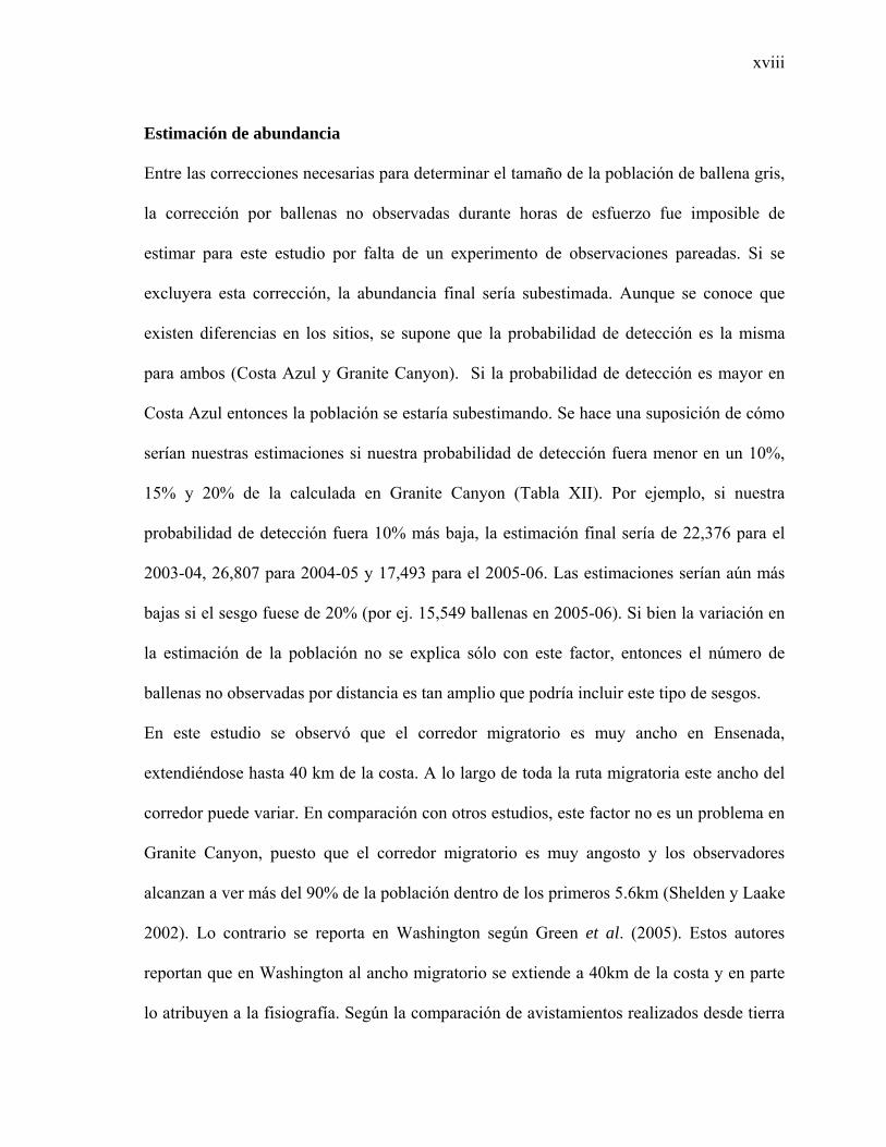
Estimación de abundancia
Entre las correcciones necesarias para determinar el tamaño de la población de ballena gris,
la corrección por ballenas no observadas durante horas de esfuerzo fue imposible de
estimar para este estudio por falta de un experimento de observaciones pareadas. Si se
excluyera esta corrección, la abundancia final sería subestimada. Aunque se conoce que
existen diferencias en los sitios, se supone que la probabilidad de detección es la misma
para ambos (Costa Azul y Granite Canyon). Si la probabilidad de detección es mayor en
Costa Azul entonces la población se estaría subestimando. Se hace una suposición de cómo
serían nuestras estimaciones si nuestra probabilidad de detección fuera menor en un 10%,
15% y 20% de la calculada en Granite Canyon (Tabla XII). Por ejemplo, si nuestra
probabilidad de detección fuera 10% más baja, la estimación final sería de 22,376 para el
2003-04, 26,807 para 2004-05 y 17,493 para el 2005-06. Las estimaciones serían aún más
bajas si el sesgo fuese de 20% (por ej. 15,549 ballenas en 2005-06). Si bien la variación en
la estimación de la población no se explica sólo con este factor, entonces el número de
ballenas no observadas por distancia es tan amplio que podría incluir este tipo de sesgos.
En este estudio se observó que el corredor migratorio es muy ancho en Ensenada,
extendiéndose hasta 40 km de la costa. A lo largo de toda la ruta migratoria este ancho del
corredor puede variar. En comparación con otros estudios, este factor no es un problema en
Granite Canyon, puesto que el corredor migratorio es muy angosto y los observadores
alcanzan a ver más del 90% de la población dentro de los primeros 5.6km (Shelden y Laake
2002). Lo contrario se reporta en Washington según Green et al. (2005). Estos autores
reportan que en Washington al ancho migratorio se extiende a 40km de la costa y en parte
lo atribuyen a la fisiografía. Según la comparación de avistamientos realizados desde tierra

xix
y desde barco en este estudio, el 56% de la población pasa más allá de la capacidad de
avistamiento de los observadores en tierra, que es de 5.5km en este estudio. Si bien las
ballenas se guían por fisiografía, la batimetría frente Ensenada y zonas adyacentes pueden
explicar el ancho del corredor migratorio (Fig. 15). Desde Rosarito (al norte de Ensenada)
se observan profundidades someras (≈100 m) que se extienden a 18 km de la costa. Estas
mismas características se observan al sur del sitio de observación, en Punta Banda y la
plataforma de Santo Tomás. Ensenada se encuentra dentro de la Bahía de Todos Santos, y
las islas Todos Santos se alinean con Punta Banda; por lo tanto, es posible que para
disminuir el gasto energético las ballenas podrían estar tomando una ruta más directa hacia
las zonas de reproducción.
El factor de corrección por distancia aumentó en 1.56 el número de ballenas en la
estimación final del estudio. Sin embargo, la corrección de ballenas no observadas en horas
de no esfuerzo también fue una fuerte contribución en la estimación. En comparación con
otros estudios en los que este factor no sobrepasa de cinco, aquí se calcularon factores que
sobrepasan el doble de esta cantidad (por ej. 12.96 en 2004-05). Estos valores altos en parte
se pueden explicar por el tiempo de esfuerzo, el cual es de sólo tres días en Ensenada y en
Granite Canyon los días de esfuerzo son el doble, y las horas de esfuerzo por día son más.
Aunque se realizaron intervalos de tiempo meticulosos, no se debe descartar que
posiblemente exista un error en la base de datos, según los intervalos de tiempo, ya que el
registro de las condiciones ambientales pudo variar según el grupo de observadores que
realizó el esfuerzo.
Aunque estos factores fueron contemplados para este estudio, el hecho de no tener una
probabilidad de detección propia del área de estudio, pudo sesgar la estimación. Este

xx
mismo factor impidió un cálculo inmediato de los coeficientes de variación (CV) de las
estimaciones. Por lo tanto, en este estudio se aproximaron CVs de 0.20, 0.35 y 0.50.
Comparando con otros estudios (Rugh et al., 2005), las estimaciones obtenidas con un CV
mayor a 0.35 arrojaron estimaciones muy bajas. Con base en esto, se podría decir que
nuestro CV se encuentra entre un 20 y 35%. Independientemente de la probabilidad de
detección, un patrón es evidente en las estimaciones de abundancia: un incremento en el
tamaño poblacional para el año 2004-05 y una disminución para la última temporada
(2005-06). Si bien es cierto que la población parece acercar su capacidad de carga o de su
equilibrio (Hobbs et al., 2004; Wade, 2002), entonces las fluctuaciones de la población
podrían ser resultado del efecto Allee, en el cual la población varía (aumenta y disminuye)
alrededor de la capacidad de carga. Son necesarios estudios más detallados para poder
mejorar la estimación de la población en Costa Azul, y entre estos detalles, cabe mencionar
que sería importante aplicar un factor de corrección por fatiga del observador.
xxi
List of contents
Page Resumen……………………………………………………………………………………. ii Abstract…………………………………………………………………………………….. iv Dedication………………………………………………………………………………….. vi Acknowledgements………………………………………………………………………... vii RESUMEN EJECUTIVO………………………………………………………………… viii List of contents…………………………………………………………………………….. xxi List of figures………………………………………………………………………………. xxiii List of tables ………………………………………………………………………………. xxvii I. INTRODUCTION…………………………………………………………….. 1 I.1. General Introduction………………………………………………………. 1 I.1a. Eastern North Pacific Gray Whale Hunting…………………………….. 3 I.1b. General Information and Importance of the Northeastern Pacific
population…………………………………………………………………. 5
I.2. Previous works…………………………………………………………….. 10 Variation in gray whale abundance…………………………………………….. 13 I.3. Rationale…………………………………………………………………... 16 I.4. Hypothesis………………………………………………………………… 17 I.5. Objectives…………………………………………………………………. 17 I.5.a. General Objective.……………………………………………………... 17 I.5.b. Specific Objectives.……………………………………………………. 17 II. METHODS…………………………………………………………………… 18 II.1. Study area………………………………………………………………… 18 II.2. Survey methods…………………………………………………………... 20 II.2a. Onshore surveys……………………………………………………….. 20 II.2b. Boat surveys…………………………………………………………… 23 II.3. Analytical methods……………………………………………………….. 27 II.3a. Migration timing……………………………………………………….. 27 II.3b. Abundance Estimation………………………………………………… 29 Diel variation………………………………………………………………. 29 Whales missed within effort hours and pod size correction……………… 29 Distance offshore………………………………………………………….. 32 Onshore theodolite tracking…………………………………………………… 32 Boat surveys……………………………………………………………………… 34 Missed whales during off-effort hours (ft)………………………………... 35 Code design for time intervals…………………………………………………. 36 Computing the correction factor ……………………………………………… 39 ..........Abundance…………………………………………………………………. 40 III. RESULTS……………………………………………………………………. 41 III.1. Migration timing………………………………………………………… 41 III.1a. Southbound migration timing…………………………………………. 45 III.1b. Northbound migration timing………………………………………… 48 III.2. Abundance Estimation…………………………………………………... 50
tf
xxii
Table of contents (continued) III.2a. Pods missed during effort hours………………………………………. 50 III.2b. Pods missed due to distance from shore……………………………… 52 Onshore theodolite tracking………………………………………………. 52 Boat surveys………………………………………………………………... 55 Comparison of onshore and boat surveys: Correction factor ( df )……… 58
III.2d. Missed whales during off-effort hours ( tf )…………………………… 62 Environmental conditions…………………………………………………. 62 III.3. Abundance………………………………………………………………. 66 IV. DISCUSSION………………………………………………………………... 68 IV.1. Migration timing………………………………………………………… 68 IV.2. Abundance estimation…………………………………………………… 71 VI.2a. Missed whales within effort hours……………………………………. 71 VI.2b Pods missed due to distance from shore………………………………. 72 VI.2c. Missed whales during off-effort periods …………………………….. 77 VI.2d. Abundance……………………………………………………………. 78 V. CONCLUSIONS……………………………………………………………... 81 VI. LITERATURE CITED……………………………………………………... 83 ANNEX I…………………………………………………………………………. 89
xxiii
List of Figures
Figure Page 1 Location of the study area at Costa Azul, Ensenada………………… 19
1 Localización del área de estudio en Costa Azul, Ensenada………..… 19
2
Classification of three known possible conditions under which the environment could yield best, acceptable, and worst environmental conditions. Basic criteria for categorized environmental conditions… 24
2
Clasificación de tres posibles condiciones bajo las cuales las condiciones ambientales pueden clasificarse como buenas, aceptables o malas. Criterios básicos para la categorización de condiciones ambientales……………………………………………… 24
3 Map showing gray whale tracking lines taken from the theodolite land surveys………………………………………………………….. 34
3 Mapa con las trayectorias de ballena gris tomadas con el teodolito de los conteos desde tierra………………………………………………. 34
4
Distribution of gray whale sightings recorded per effort hour during the three surveyed seasons (2003-2006). Black = southbound, pink = northbound without calves, and yellow = northbound cow/calf pairs…………………………………………………………………... 43
4
Distribución de avistamientos de ballena gris por hora de esfuerzo para cada una de las tres temporadas (2003-2006). Negro = sur, rosado = norte sin crías y amarillo = norte parejas hembra/cría……………………………………………….………..…. 43
5
Distribution of northbound migrating whales sighted per hour of effort during the three surveyed seasons (2003-2006), including cow/calf pairs. a) Whales without calves, b) cow/calf pairs…………. 44
5
Distribución del número de ballenas registradas por hora de esfuerzo en la migración al norte durante las tres temporadas de muestreo (2003-2006). a) Ballenas sin crías, b) parejas madre/cría……………………………………………………………. 44
xxiv
List of Figures (continued)
6 Distribution of southbound gray whales sighted per effort hour during the three surveyed seasons. Time is shown from 01-Dec. to 15-Mar………………………………………………………………... 46
6
Distribución de avistamientos de ballena gris por hora de esfuerzo en la migración al sur para las tres temporadas de muestreo, del 1 de diciembre al 15 de marzo…………………………………………….. 46
7
Comparison of the distribution of sightings per distance interval obtained from onshore theodolite tracking at Costa Azul (black = 2003-04; gray = 2004-05; light gray = 2005-06) with the results from aerial surveys at Granite Canyon, California (dotted bars) (Shelden and Laake, 2002)……………………………………………………... 54
7
Comparación de la distribución de los avistamientos obtenidos con el teodolito desde tierra en Costa Azul, según el intervalos de distancia, (negro = 2003-04; gris = 2004-05; gris claro = 2005-06) y los resultados de recorridos aéreos en Granite Canyon, California (barras punteadas) (Shelden y Laake, 2002)…………………………………. 54
8 Offshore distance of gray whale sightings per distance interval according to boat survey results……………………………………… 56
8 Proporción de avistamientos de ballena gris según los intervalos de distancia de la costa registrados desde el barco……………………… 56
9 Distribution of percent sightings obtained within 5.54km from shore and divided into 1.3705km intervals (0.74nm), to compare with results from Shelden and Laake’s (2002) aerial surveys at Granite Canyon, California…………………………………………................ 57
9 Distribución del porcentaje de avistamientos dentro de los primeros 5.54km de la costa y divididos en intervalos de 1.3705km (0.74nm), para comparar con los resultados de censos aéreos en Granite Canyon, California, por Shelden y Laake (2002)…………………..… 57
10
Cumulative percent sightings from boat surveys and those obtained from land with the theodolite (per season). More than 50% of boat sightings were recorded beyond 5.5km, the distance at which the shore observer is able to record with the theodolite.………………………………………….…………………. 60

xxv
List of Figures (continued)
10
Porcentaje acumulado de los avistamientos obtenidos de barco y desde tierra con el teodolito (por temporada). Más del 50% de avistamientos desde barco se registran a más de 5.5km, distancia máxima a la que el observador en tierra logra registrar con el teodolito………………………………………………………….…. 60
11 Cumulative percent sightings from boat surveys and those obtained from land with the theodolite (per season). More than 50% of boat sightings were recorded beyond 5.5km, the distance at which the shore observer is able to record with the theodolite………………….. 61
11
Porcentaje acumulado de los avistamientos obtenidos de barco y desde tierra con el teodolito (por temporada). Más del 50% de avistamientos desde barco se registran a más de 5.5km, distancia máxima a la que el observador en tierra logra registrar con el teodolito………………………………………………………………. 61
12 Fitted distribution (using Hermite polynomials) of estimated number of whales per day passing the survey site for the 2003-04 season (solid line)……………………………………………………………. 63
12
Figura 12. Distribución ajustada (utilizando polinomios de Hermite) del número estimado de ballenas que pasaron por el sitio de observación en la temporada 2003-04 (línea continua)……………… 63
13 Fitted distribution (using Hermite polynomials) of estimated number of whales per day passing the survey site for the 2004-05 season (solid line)…………………………………………............................. 64
13 Distribución ajustada (utilizando polinomios de Hermite) del número estimado de ballenas que pasaron por el sitio de observación en la temporada 2004-05 (línea continua)…………………………………. 64
14
Fitted distribution (using Hermite polynomials) of estimated number of whales per day passing the survey site for the 2005-06 season (solid line)……………………………………………………………. 65
14
Distribución ajustada (utilizando polinomios de Hermite) del número estimado de ballenas que pasaron por el sitio de observación en la temporada 2005-06 (línea continua)…………………………………. 65
xxvi
List of Figures (continued)
15
Bathymetry map south of the observation site showing Santo Tomás shelf and Soledad Ridge. This study’s observation point is located near punta Salsipuedes (Legg, 1985)………………………………… 74
15
Mapa batimétrico del sur del sitio de observación mostrando la plataforma de Santo Tomás y la cresta de la Soledad. El punto de observación de este estudio se localiza cerca de punta Salsipuedes (Legg, 1985)………………………………………………………….. 74
16
Gray whale population size time series from studies at Granite Canyon taken from Alaska Marine Mammal Stock Assessment (2005), including the estimates in this study (squares). Confidence intervals were not calculated; however, a conservative 35% coefficient of variation is shown…………………………………….. 79
16
Serie de tiempo del tamaño de la población de la ballena gris tomado de Alaska Marine Mammal Stock Assessment (2005), incluyendo las estimaciones de este estudio (cuadros). No se calcularon intervalos de confianza; sin embargo, se muestra un coeficiente de variación conservador del 35%............................................................................. 79
xxvii
List of tables
Table Page
I Reticle distance values used in this study after Kinzey and Gerrodette (2001)………………………………………………………... 26
I Valores de la distancia de las retículas utilizados en este estudio de acuerdo a Kinzey y Gerodette (2001)…………………………………... 26
II
Classification of three known possible conditions under which the environment could yield best, acceptable, and worst environmental conditions. Basic criteria for categorized environmental conditions……… 38
II
Clasificación de tres posibles condiciones bajo las cuales las condiciones ambientales pueden clasificarse como buenas, aceptables o malas. Criterios básicos para la categorización de condiciones ambientales…….. 38
III
Code criteria, based on environmental factors, for three categorized conditions. Categories show the conditions required to yield a respective code. Percent values reflect percent sighting frequencies under the respective environmental condition. (Swell: 0=absent and 1=presence)…. 38
III
Criterios para códigos, basados en los factores ambientales para tres condiciones categorizadas. Las categorías muestran las condiciones necesarias para llegar a su respectivo código. El valor porcentual refleja la frecuencia de avistamientos bajos la condición ambiental respectiva. (Mar de fondo: 0=ausencia y 1=presencia)……………………………….. 38
IV Effort times are given for each migration season as well as the number of pods and whales counted during the southbound surveys……………….... 41
IV
Tiempo de esfuerzo para cada temporada así como el número de grupos de ballenas y el total de ballenas contadas durante los conteos de la migración al sur…………………………………………………………… 41
V
Dates of occurrence of the tails of the southbound migration and median dates (50%) taken from the relative abundance index, for each migration season……………………………………………………………………… 47
V
Fechas de las proporciones extremas (10% y 90%) de la migración al sur y fechas medianas (50%), tomadas del índice de abundancia relativa para cada temporada……………………………………………………………. 47
xxviii
List of tables (continued)
VI Mean relative abundance index showing whales per hour during the three migration seasons (2003-2006)…………………………………………… 47
VI Índice promedio de abundancia relativa mostrando numero de ballenas por hora durante las tres temporadas de migración (2003-2006)…………. 47
VII Dates of percent sightings obtained during the northbound migration in every season; no cow/calf pairs…………………………………………… 49
VII Fechas del porcentaje de avistamientos registrados en la migración al norte durante cada temporada; sin crías…………………………………… 49
VIII Dates of percent sightings obtained during the northbound migration in every season; cow/calf pairs………………………………………………. 50
VIII Fechas del porcentaje de avistamientos registrados en la migración al norte durante cada temporada; sólo parejas madre/cría…………………… 50
IX
Estimation of total number of whales passing the survey site (W ), in each surveyed season, using corrections for missed pods within effort periods and pod size bias due to observers as reported in Rugh et al. (2005). eW = No. whales in pods of size e…………………………………………….. 51
IX
Estimación del total de ballenas que pasaron el sitio de observación (W ), en cada temporada, utilizando las correcciones para grupos no observados dentro de horas de esfuerzo y sesgo de los observadores por tamaño de grupo, tal como lo reportan Rugh et al. (2005). eW = No. ballenas en grupos de tamaño e………………………………………………………... 51
X
Number and percent of tracked sightings recorded per distance interval during each surveyed season. Chi square tests revealed a significant difference in the number of sightings between intervals for every year (p<0.001)………………………………………………………………….. 53
X
Número y porcentaje de avistamientos registrados según el intervalo de distancia. La prueba ji-cuadrada mostró diferencias significativas en el número de avistamientos entre los intervalos para cada año (p<0.001)…... 53
xxix
List of tables (continued)
XI
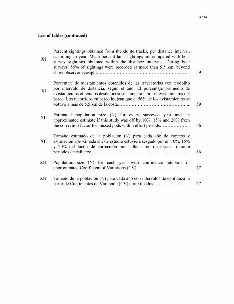
Percent sightings obtained from theodolite tracks, per distance interval, according to year. Mean percent land sightings are compared with boat survey sightings obtained within the distance intervals. During boat surveys, 56% of sightings were recorded at more than 5.5 km, beyond shore observer eyesight……………………………………………………. 59
XI
Porcentaje de avistamientos obtenidos de las trayectorias con teodolito por intervalo de distancia, según el año. El porcentaje promedio de avistamientos obtenidos desde tierra se compara con los avistamientos del barco. Los recorridos en barco indican que el 56% de los avistamientos se obtuvo a más de 5.5 km de la costa……………………………………….. 59
XII
Estimated population size (N) for every surveyed year and an approximated estimate if this study was off by 10%, 15% and 20% from the correction factor for missed pods within effort periods……………….. 66
XII
Tamaño estimado de la población (N) para cada año de conteos y estimación aproximada si este estudio estuviera sesgado por un 10%, 15% y 20% del factor de corrección por ballenas no observadas durante periodos de esfuerzo………………………………………………………. 66
XIII Population size (N) for each year with confidence intervals of approximated Coefficient of Variations (CV)…………………………….. 67
XIII Tamaño de la población (N) para cada año con intervalos de confianza a partir de Coeficientes de Variación (CV) aproximados………………… 67

I. INTRODUCTION
I.1. General Introduction
The eastern Pacific gray whale (Eschrichtius robustus; Lilljeborg, 1861) is a
cetacean belonging to the Eschrichtiidae family. As a mysticete, or baleen whale, grays
share similarities with other great whales yet they have unique physical and demographic
characteristics. Among these, there is the long annual migration they make, along the
western coasts of the North American continent which in turn is convenient for its
monitoring.
Specifically, the eastern Pacific stock has been monitored ever since it was first
considered endangered due to whale hunting and its recovery has been followed up-to-date
with modeled census data and population size estimates. Whaling has seized for this stock
and today the gray whale is only hunted for subsistence by aboriginal groups with a limited
annual quota. The quota is stated by the International Whaling Commission and the
feedback for this decision comes, in part, from abundance estimates.
Population estimates have been assessed by the National Marine Mammal
Laboratory in California (U.S.), nevertheless, the long migratory route of the Eastern
Pacific gray whale stock makes us consider it as a common resource shared among three
nations: Canada, United States, and Mexico. It is hard enough to assess a resource
belonging to one sole nation; therefore, assessment becomes more complex when it comes
to a shared resource. Despite the agreement among the nations, the basic path for a good
assessment is through the knowledge of the resource’s health and status, as well as the
2
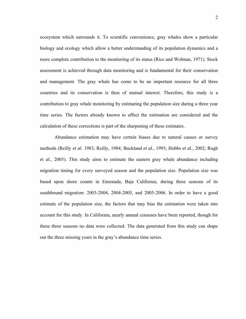
ecosystem which surrounds it. To scientific convenience, gray whales show a particular
biology and ecology which allow a better understanding of its population dynamics and a
more complete contribution to the monitoring of its status (Rice and Wolman, 1971). Stock
assessment is achieved through data monitoring and is fundamental for their conservation
and management. The gray whale has come to be an important resource for all three
countries and its conservation is then of mutual interest. Therefore, this study is a
contribution to gray whale monitoring by estimating the population size during a three year
time series. The factors already known to affect the estimation are considered and the
calculation of these corrections is part of the sharpening of these estimates.
Abundance estimation may have certain biases due to natural causes or survey
methods (Reilly et al. 1983; Reilly, 1984; Buckland et al., 1993; Hobbs et al., 2002; Rugh
et al., 2005). This study aims to estimate the eastern gray whale abundance including
migration timing for every surveyed season and the population size. Population size was
based upon shore counts in Ensenada, Baja California, during three seasons of its
southbound migration: 2003-2004, 2004-2005, and 2005-2006. In order to have a good
estimate of the population size, the factors that may bias the estimation were taken into
account for this study. In California, nearly annual censuses have been reported, though for
these three seasons no data were collected. The data generated from this study can shape
out the three missing years in the gray’s abundance time series.

3
I.1a. Eastern North Pacific Gray Whale Hunting
Gray whale populations are clear examples of what has happened, what is
happening, and what would happen with an exploitable resource depending on the
assessment and management it is given. Gray whaling history portrays the importance of
assessing a resource and taking conservation measures.
At the beginning of the nineteenth century, when Pacific whale stocks were
discovered by American and European whalers, one of the stocks to be severely affected
was that of the gray whale. Although they knew it was one of the most dangerous whales to
hunt because of its aggressive reactions to hunters (especially mothers protecting calves),
whalers went after it for its high commercial revenue (Henderson, 1984). Three gray whale
(Eschrichtius robustus; Lilljeborg, 1861) stocks were distributed along the northern
hemisphere before whaling occurred: Eastern Pacific stock, Western Pacific stock (found
on the eastern coast of Asia) and the Atlantic stock (possibly distributed throughout the
northern Atlantic Ocean). Intense whaling extinguished the Atlantic stock, and today only
two geographically separated gray whale stocks are recognized with a limited distribution
along the eastern and western coasts of the Northern Pacific Ocean (Rice and Wolman,
1971).
Excessive unsupervised whaling was probably the main contributor to the extinction
of the North Atlantic gray whale population in the early 17th century (Bryant, 1995), and
Pacific gray populations were both nearing the same fate. When the eastern Pacific grays
were going through depletion in the mid 19th century, the Korean stock remained “intact”
(Mizue, 1951). Uncontrolled whaling activities and lack of management later exhausted the
4
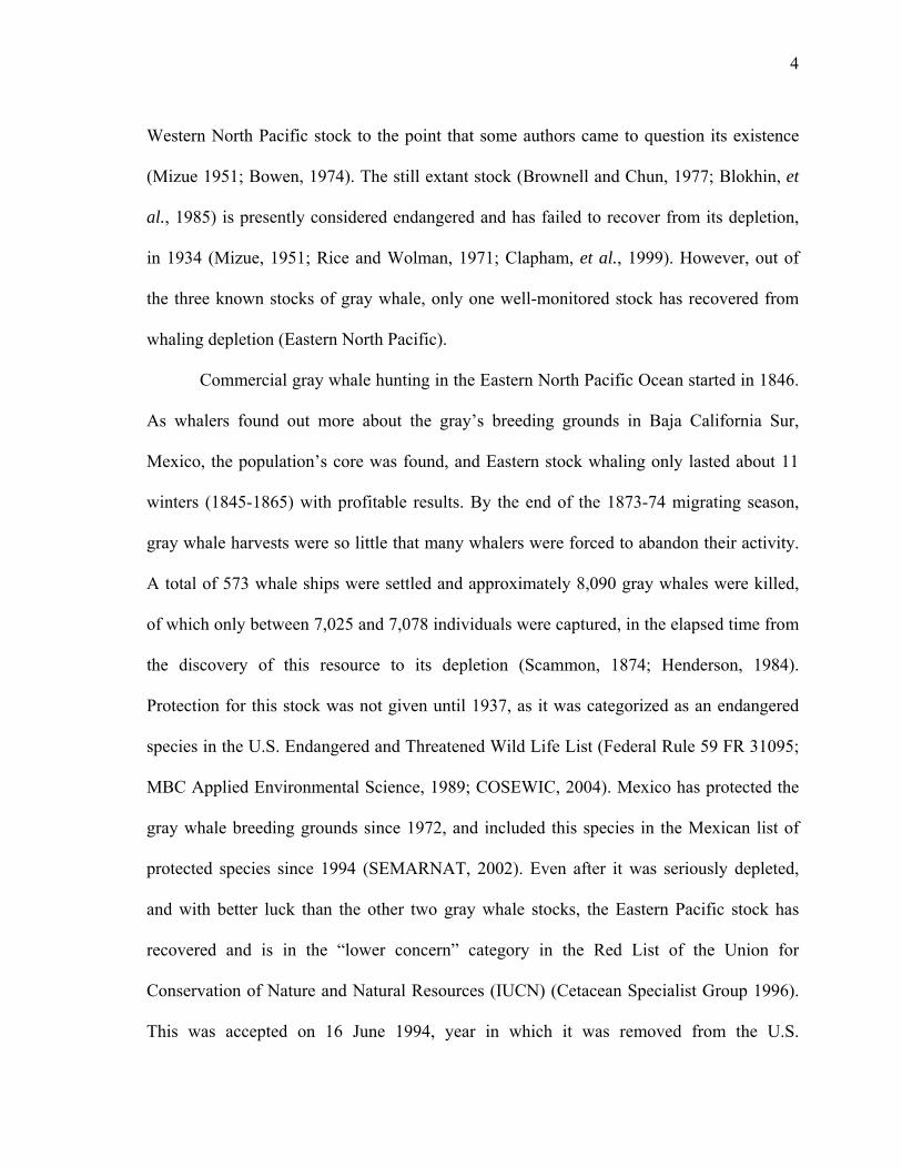
Western North Pacific stock to the point that some authors came to question its existence
(Mizue 1951; Bowen, 1974). The still extant stock (Brownell and Chun, 1977; Blokhin, et
al., 1985) is presently considered endangered and has failed to recover from its depletion,
in 1934 (Mizue, 1951; Rice and Wolman, 1971; Clapham, et al., 1999). However, out of
the three known stocks of gray whale, only one well-monitored stock has recovered from
whaling depletion (Eastern North Pacific).
Commercial gray whale hunting in the Eastern North Pacific Ocean started in 1846.
As whalers found out more about the gray’s breeding grounds in Baja California Sur,
Mexico, the population’s core was found, and Eastern stock whaling only lasted about 11
winters (1845-1865) with profitable results. By the end of the 1873-74 migrating season,
gray whale harvests were so little that many whalers were forced to abandon their activity.
A total of 573 whale ships were settled and approximately 8,090 gray whales were killed,
of which only between 7,025 and 7,078 individuals were captured, in the elapsed time from
the discovery of this resource to its depletion (Scammon, 1874; Henderson, 1984).
Protection for this stock was not given until 1937, as it was categorized as an endangered
species in the U.S. Endangered and Threatened Wild Life List (Federal Rule 59 FR 31095;
MBC Applied Environmental Science, 1989; COSEWIC, 2004). Mexico has protected the
gray whale breeding grounds since 1972, and included this species in the Mexican list of
protected species since 1994 (SEMARNAT, 2002). Even after it was seriously depleted,
and with better luck than the other two gray whale stocks, the Eastern Pacific stock has
recovered and is in the “lower concern” category in the Red List of the Union for
Conservation of Nature and Natural Resources (IUCN) (Cetacean Specialist Group 1996).
This was accepted on 16 June 1994, year in which it was removed from the U.S.
5
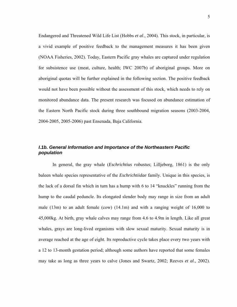
Endangered and Threatened Wild Life List (Hobbs et al., 2004). This stock, in particular, is
a vivid example of positive feedback to the management measures it has been given
(NOAA Fisheries, 2002). Today, Eastern Pacific gray whales are captured under regulation
for subsistence use (meat, culture, health; IWC 2007b) of aboriginal groups. More on
aboriginal quotas will be further explained in the following section. The positive feedback
would not have been possible without the assessment of this stock, which needs to rely on
monitored abundance data. The present research was focused on abundance estimation of
the Eastern North Pacific stock during three southbound migration seasons (2003-2004,
2004-2005, 2005-2006) past Ensenada, Baja California.
I.1b. General Information and Importance of the Northeastern Pacific population
In general, the gray whale (Eschrichtius robustus; Lilljeborg, 1861) is the only
baleen whale species representative of the Eschrichtiidae family. Unique in this species, is
the lack of a dorsal fin which in turn has a hump with 6 to 14 “knuckles” running from the
hump to the caudal peduncle. Its elongated slender body may range in size from an adult
male (13m) to an adult female (cow) (14.1m) and with a ranging weight of 16,000 to
45,000kg. At birth, gray whale calves may range from 4.6 to 4.9m in length. Like all great
whales, grays are long-lived organisms with slow sexual maturity. Sexual maturity is in
average reached at the age of eight. Its reproductive cycle takes place every two years with
a 12 to 13-month gestation period; although some authors have reported that some females
may take as long as three years to calve (Jones and Swartz, 2002; Reeves et al., 2002).
6
This, however, turns out to be quite inconvenient for the growth of a population, since it
makes it more vulnerable to depletion, which in turn may bring about negative effects on
the zones it inhabits.
Particularly, Eastern Pacific grays are known for setting the longest migration route
than any other mammal in one long period of time (Rice and Wolman, 1971). They migrate
around 8,000km from Unimak Pass (Alaska) all the way through to the winter breeding
grounds in the Baja California lagoons in Mexico in approximately 54 days, and an even
longer time and path for those coming from the Beaufort Sea traveling more than 10,000km
(Rugh et al., 2001). As a migratory species, gray whales have a broad distribution all along
the western coasts of the North American continent. During the summer, they feed on the
shallow Bering, Chukchi and Beaufort Sea floors to be able to take on their annual
migration. Feeding only occurs in the summer; grays generally do not feed during the entire
migration period (Rice and Wolman, 1971) though they have been observed feeding along
the route (Le Boeuf et al., 2000; Rugh et al., 2001). Therefore, it is important for them to
forage plenty of energy in order to make it back to the feeding grounds. This is especially
essential for pregnant females which must feed their calves at the breeding grounds.
The long trip for grays starts in autumn, at the beginning of October and November,
although they have left the feeding grounds as late as September (Rugh et al., 2001). The
first whales to leave the feeding grounds past Unimak Pass are pregnant females, second
are adult males, followed by immature females and lastly immature males (Rice and
Wolman, 1971). From Unimak Pass, they go past the Aleutian Islands and head south along
the Canadian and United States coasts. By December, they accomplish the first half of their
migration journey in Mexican lagoons and bays along the western Baja California region
7
(Rice and Wolman, 1971) to reproduce and give birth to new recruitment (calves). The
main breeding zones are Guerrero Negro, Ojo de Liebre, and San Ignacio lagoons, and
Magdalena bay, although some whales have also been reported as far south as Cabo San
Lucas and in the Gulf of California (Gilmore et al., 1967; Rice and Wolman, 1971; Reilly,
1984; Findley and Vidal, 2002).
Migration back to the feeding grounds starts in February, although some whales
have been spotted still on their southbound migration during that time (Rugh et al., 2001).
This time, conceived females are the first to leave the breeding grounds back to the feeding
grounds followed by adult males, behind them are mestrous, anestrous, and immature
females, and right after them are all immature males (Rice and Wolman, 1971). It is worth
mentioning the importance for conceived females to get to the feeding areas before all the
other whales, since they are in a pregnancy state (embryo development). The last whales to
leave Mexican waters are females with calves (cow/calf pairs). These whales and their
youngsters remain a longer period of time in Mexican lagoons, feeding, nursing, and
preparing them for their long journey back to the feeding grounds. In general, the
northbound migration, which lasts about 3 months, is slower than the 2-month southbound
migration (Pike, 1962).
Gray whales from the Eastern Pacific stock are of great importance in benthic-arctic
ecosystems, due to the ocean floor modifications it causes with its feeding strategies. They
feed every summer on the Arctic benthos, preferably amphipods buried in the ocean floor.
Hence, frequent disturbance on these ocean floors, caused by feeding, is followed by
succession of benthic organisms (Oliver and Slattery, 1985; Highsmith and Coyle, 1992; Le
Boeuf et al., 2000). This feeding ground is one of the most productive areas worldwide

8
(Springer, 2000). Considering the number of whales feeding there and the amount of food
consumption required by their metabolism, the removal of this stock could cause greater
abundance of benthic organisms, leading to space competition, among other possible
derived causes. In fact, the gray whale has even been stated as a keystone species of arctic
benthic communities for maintaining its structure on the invertebrates it feeds upon (Oliver
and Slaterry, 1985). Biologically and ecologically, they play an important role in ocean-
floor modifications, structurally modifying its feeding ecosystem and are hosts to many
parasites (mainly barnacles; Cryptolepas rhachianecti). In fact, out of all great whales,
grays are the most parasitized (Jones and Swartz, 2002). The importance of these animals
goes beyond its ecological magnitude. COSEWIC (2004) state a cultural and economic
importance, of which the cultural importance will be slightly discussed later on and the
economic importance relies mainly on whale watching, especially at the summer and winter
grounds.
Gray whale abundance may determine that of other organisms, especially those in
benthic communities in the arctic zone, due to its feeding strategies (Oliver and Slattery,
1985; Highsmith and Coyle, 1992); therefore, the source of its abundance variation itself
should be of concern. Gray whale abundance may vary depending on the nature of the
causes. Naturally speaking, these variances may be due to climatic conditions; current
climate change, El Niño and La Niña events, among other causes (Le Boeuf et al., 2000).
Anthropogenic causes are the second nature of whale abundance variability. A third cause
of population decline may be due to incidental deaths caused by fishing operations (Baird et
al., 2002) or aboriginal subsistence whaling, as mentioned earlier.
9
Although commercial whaling is no longer permitted, subsistence whaling still
takes place and is of great cultural importance to some aboriginal groups in the Northern
part of North America and along the Siberian coasts. Understanding the importance of
subsistence whaling for these aboriginal groups, this type of whaling is limited to aboriginal
groups in Alaska and the eastern coast of Russia (NOAA Fisheries, 2002; IWC, 2007a and
b).
Stock assessment is a means of stock status monitoring (abundance, maximum net
production rate, population trends), and so management decisions regarding its actual status
or subsistence whaling quotas may be determined. The International Whaling Commission
(IWC, 2007a) had previously established the eastern stock quota to be an average of 120
individuals caught per year and it would be valid and intact through a five-year period
(2003-07). Up-to-date, subsistence whaling is restricted to a harvest quota, split among the
Alaskan and Siberian aborigines of the two countries (USA and Russia), of 620 whales in a
five-year period from 2008-2012. A maximum of 140 individuals can be harvested in one
of these years (IWC, 2007a and 2007d). Depending on the annual harvest, the quota for the
following year is determined and it shall not exceed 140 individuals nor shall this harvest
be repeated during the five-year period. In order to establish the above five-year total
harvest, the IWC needs information to base upon and decide over aboriginal whaling
quotas. Information on abundance estimates can give a general idea of population behavior
and perhaps an idea on the population’s health.
10
I.2. Previous works
Before methods used nowadays, one of the main sources to determine whale
populations was through catch per unit of effort information (CPUE; Allen, 1980). Methods
evolved, and today the main source for assessing whale populations is through direct
observations from shore, boat, and/or aerial means (Hubbs and Hubbs, 1967; Gard, 1974;
Reilly et al., 1983; Reilly, 1984; Green et al., 1995; Shelden and Laake, 2002). In
California, onshore census surveys have been taking place since 1967. However, the
eastern population of gray whales was first surveyed in 1887 by Townsend (Reilly, 1984).
Townsend (1887) was one of the pioneers to point out the factors that influence total
abundance estimation based on onshore counts: unseen whales passing during the night,
before and after a census takes place, and those whales passing way beyond the observer’s
visual sight. At that time, these factors were solely a concern. With time, methods to
account for these discrepancies were developed and improved to near abundance estimates
as close as possible to true population abundance.
Reilly et al. (1980) made a preliminary estimate of the gray whale eastern Pacific stock
based on a 12-year observation effort. The main concerns in their study were observer bias,
what percent of the population was passing beyond the observer’s eye sight, and diel and
weather variation. Their research fully explored the first two concerns, the other two
remained unexplored. Later, in 1983, Reilly et al. published an assessment for this
population adding one more year to their previous study in Reilly et al. (1980), analyzing
13 years. Their study took into account those factors that may bias the estimation of the
population. In order to certain their estimate, they point out the possibility of bias due to

11
diel variation. Unfortunately this latter factor was not proven by them, given that there was
a bias on the first hour of the census. The estimation to correct for this factor was pioneered
with the study of Swartz et al. (1987). Buckland et al. (1993) used this information to
correct for the travel rate inconsistency ( ) and they found that the whales’ travel speed
was slightly faster at night ( = 1.020). Later in 1999, Perryman et al., edged this
correction after running a thermal imagery experiment. Though they found similar results
in travel rates, they complemented the study by contemplating data containing the fraction
of whales migrating after the median date (when 50% of the sightings are reported) rather
than a “fixed calendar day” (15 January). The newly estimated correction factor ( =
1.0875) has been used in recent abundance estimations (Rugh et al., 2005).
*nf
*nf
*nf
Observer discrepancies occur and were first studied in Reilly et al. (1980) in California. An
experiment of data comparison between observations made by 12 observers making
individual counts and data taken as “true counts” from simultaneous observations made
during aircraft surveys was the first step to consider this bias. Furthermore, in 1990, Rugh
et al. conducted new experiments making paired independent counts at Granite Canyon,
California, during the peak of the 1986 southbound migration season (effort time 60 hr).
Their results showed that a great percentage of whales was being missed within the viewing
area by single observers. In their study, they found that of all whales passing the viewing
area, 21% was being missed or uncounted by observers and that a greater percent of whales
was missed than groups were undercounted. This study was only based on a 6-day
experiment. Rugh et al. (1993) extended and sharpened this research, again, using a “mark-
recapture” experiment, though this time effort consisted in a complete 2-month period. A
12
scoring algorithm was devised to match sightings and find the percent sightings being
missed. Similar results, comparing with Rugh et al. (1990), were found in this study, as
they found that most seen whales were within a 1.5 to 4.4km offshore range (Rugh et al.,
1990, report a range of 0.5 to 3.7 km offshore). The number of whales missed by observers
was found to be 19%.
Sighting records have also shown that observers miss a percent of whales because of
distance from shore. Boat and aerial experiments have been used to correct for this missed
percentage. Reilly et al. (1980) flew an aircraft running parallel transect line surveys,
perpendicular to the coast near the Granite Canyon survey station in California. As a result,
they reported that 90% of grays were passing within 2 n.m. of their research station.
Shelden and Laake, (2002) later obtained different results in their aerial surveys. They
conducted 6 aerial surveys near Granite Canyon, at the same time onshore surveys took
place, during the peak of the southbound migration in 1996. Most of their observations
were within 3 n.m. Green et al. (1995) followed a similar experiment in Oregon and
Washington in 1990 to find the gray whale’s migration corridor. Contrary to other known
survey sites, the whale’s migration corridor was very wide. Most of the gray whales were
passing beyond 10 km from the coast (66%). At the same time, whales were passing further
offshore (13 km) at Washington than at Oregon. Aerial surveys provide means to determine
the migration corridor; hence, if needed, correct for a percent of whales missed due to
distance. However, they are very costly, and might not always fit in the budget. Rugh et al.
(2002) conducted paired independent surveys using fix-mounted 25-powered binoculars to
evaluate yearly variations in migration corridors (offshore distribution). They suggested
this method as an alternative to aerial surveys.

13
Distance from shore can also be analyzed from boat surveys. Due to the different
conditions, the equipment used in boat surveys is a Global Positioning System, an angle
board and binoculars edged with reticles. Kinzey and Gerodette (2003) present “accuracy
and precision of distances measured at sea.”
Observations are not possible all 24 hours. There are times in which no effort can be
undertaken. Calculation for this factor first consisted in fitting a normal density curve of
sightings with a gamma function (Reilly, 1983). These calculations were eased later on by
Buckland (1992) with the introduction of the use of Hermite polynomial extrapolation to
account for missed periods. This method was again used in abundance estimations in
Buckland et al. (1993) and this has been the method used up to recent studies.
Variation in gray whale abundance
Reilly et al. (1983) concluded that the population had an annual increase of 2.5%. Although
there was an annual increase rate, these authors reported a season of low estimates (1971-
72) and they attributed it, in part, to poor visibility due to a “stormier year” than usual.
According to Reilly et al. (1983), NOAA Fisheries (2002) and the Committee on
the Status of Endangered Wildlife in Canada (COSEWIC, 2004) reports, the eastern gray
whale stock has a mean annual increase of 2.5%. On the other hand, serious death increases
have also been reported for certain years (Le Boeuf et al., 2000; Gulland et al., 2005; IWC,
2007c), and also a recent delay in its onset migration time (Rugh et al., 2001). High
mortalities and low recruitments both coincided in the 1998-99 season (Le Boeuf et al.,
2000). Mortalities reported during the 1998-99 season “exceed any other reported in
previous years” down to 1985 (Le Boeuf et al., 2000). During 1975-2006, IWC (2007c)
14
reports 1,892 stranded whales along its migratory route. Two stranding peaks can be
pointed out during the time series from 1985 to 1999: one in 1991 and a second one in
1999. It is well-known that females compose an important part of a population’s
recruitment and the strandings for those seasons, according to Le Boeuf et al. (2000), were
mainly females. Female losses may lower the incoming components of a population
(recruitment) and so it was seen that calf recruitment was a low 1.7% compared to a
variable 4.6-4.7% in previous years (Perryman et al., 2002). Also, when observers expected
to sight twice the number of mothers and calves in March (i.e. 92 in 1996 mother/calf
pairs), during the study reported in 2002, they only observed in average 45 mother/calf
pairs (Le Boeuf et al., 2000).
High mortalities were also followed in the subsequent year with a 1.1% recruitment
rate (COSEWIC, 2004 and Le Boeuf et al., 2000). Despite this decrease, death rates went
back to normal in 2001 (Perryman, 2002), notwithstanding that the annual recruitment was
still low at 1.4%. Totally different rates were reported for 2002 and 2003 with percentages
of 4.8 and 4.4% respectively (COSEWIC, 2004). The population estimates, however, for
2001 and 2002, were 18,761 individuals for 2001, and 17, 414 for 2002 (Rugh et al., 2005).
The population for 2002 still showed a decrease in number despite its recruitment increase.
The latter resulted in a 10% population decrease since 1998 (COSEWIC, 2004).
Le Boeuf et al. (2000), Springer (2000), and Rugh et al. (2001) agreed on a
starvation conclusion due to climate shifts. They also reported a change in primary
productivity as an effect of global warming. It is agreed that a shift in primary productivity
will affect, in turn, benthic communities. Le Boeuf et al. (2000) cited 3 authors (giving
information on arctic productivity) of which Springer (2000) reports a 30% decrease in the

15
past 30 years for the Chukchi-Bering ecosystem. Other possible climatic effects are
reported in Le Boeuf et al. (2000) with a relation found between sea surface temperatures
and El Niño, which may be, in part, a plausible cause of the decline in the Bering Sea
amphipod communities.
NOAA Fisheries (2002) states an annual Potential Biological Removal1 for this
stock of 575 individuals, which is based upon a minimum number of individuals. It is also
reported that this number is not exceeded by the total number of individuals killed
incidentally by fishing operations and the aboriginal hunt summed together.
The eastern gray whale stock has considerably reduced in numbers during three
consecutive years, since 1999. It is quite known that without recruitment, growth, in any
population, will be poor. Therefore, low recruitment in the mentioned years could be
contributing to the 10% decrease COSEWIC (2004) reports.
As an observation from past estimates (1999-2002), recruitment has been seriously
affected. Mean birth rate in Eschrichtius robustus is one calf per adult (twins are rare) and
it presents a biennial reproductive cycle (Rice y Wolman, 1971). This implies a constant
monitoring for this stock due to its ecologic importance and the fact that aboriginal groups
depend on it as well. Regardless of the nature of deaths, populations are being varied either
by anthropogenic causes or as in recent years (such as the high mortalities in 1999) by
natural causes. This is true for almost, if not all populations, since they are never constant,
rather they are always changing and need constant monitoring.
1 According to NOAA Fisheries (2002), “the Potential Biological Removal is defined as the product of the minimum population estimate, one-half the maximum theoretical net productivity rate, and a recovery factor.”

16
I.3. Rationale
Aside from being one of the basic parameters in studying and learning about the
dynamics of a population, abundance is also important and necessary in resource
assessment. It is quite true, as mentioned earlier, that populations are not constant, and this
is evident in the fluctuations of gray whale abundance throughout its known history.
Just when it was thought that the population had recovered from depletion and in
addition that it had reached its carrying capacity, the eastern gray whale stock went through
important decreases in the past years (Rugh et al., 2005). Besides effects on the Bering-
Chukchi ecosystem, aboriginal groups that depend on this resource would also be seriously
affected, should this resource be negatively altered in numbers.
The information up-to-day of census data is available only until 2002. This study
will bring out an idea of the population fluctuation on the subsequent three seasons (2003-
2006) lacking census efforts on the population at Granite Canyon, California. It is also very
important to note that related studies, in the understanding of gray whale abundance, are
almost inexistent in the southern part of its migration route in Mexican waters, with the
exception of the calving areas. The Baja California peninsula is, in particular, an important
region for the recruitment of this population, and as a country partially responsible for this
resource, it is important for it to develop its own data to aid in the knowledge of what is
also its resource. Hence, it would also develop its own back-up information and this study
should be a preliminary contribution of gray whale abundance in Mexico.
17
I.4. Hypothesis
The gray whale eastern Pacific stock has gone through some important changes.
Springer (2002) reports a 30% decrease in the Bering-Chukchi ecosystem in the past 30
years. Therefore, this stock could possibly have continued diminishing since 2002, last
census-reported year in California.
I.5. Objectives
I.5.a. General Objective:
In order to generate new information in Mexico and in the time series regarding the gray
whale’s annual population abundance, this study focused on the estimation of gray whale
abundance of the eastern Pacific stock during its southbound migration in three seasons
(December to May 2003-2004, 2004-2005, and 2005-2006).
I.5.b. Specific Objectives:
• To determine the south and northbound migration timing (beginning, peak, and end)
in Ensenada based upon a relative abundance index (number of
individuals/observation hour).
• To estimate the population size of the gray whale based upon onshore counts during
three southbound seasons (2003-2004, 2004-2005, and 2005-2006) along with the
correction factors that influence and affect the final estimation.
18
II. METHODS
II.1. Study area
Surveys took place about 23km north of Ensenada at Costa Azul. Costa Azul is
situated on the northwestern side of the Baja California peninsula, Mexico, at 31º 58”95’N,
116º 50”16’W (Fig. 1). The Ensenada region falls within the Southern California Bight,
since the latter extends from Point Conception, California (USA), to Punta Colonet, Baja
California. (Hickey, 1993). The continental shelf coasting the Ensenada region extends 2km
from the coastline, dropping into a steep continental slope ≈ 360 m deep (CSDS, 1971).
The port of Ensenada is located within Todos Santos Bay, having a small peninsula (Punta
Banda) protuberating from the coastline. North of Punta Banda lies a steep 550m-deep
submarine canyon, separating Punta Banda from the Todos Santos volcanic islands
(Heckel, 2001; CSDS, 1971).
Weather in the study area is Mediterranean-like; dry in the summer and rainy in the
winter. Annual mean temperature is 16.5°C though it ranges from 14.0°C in December to
16.3°C in May (elapsed time of a survey season). The lowest mean temperatures are given
in January with 13.3°C. Precipitation is highest in January (42.5mm) and in May it lowers
to 3.4mm totaling 190.4mm annually. Wind also plays an important role in this region.
Annually, from September through May, polar wind masses prevail (Energía Costa Azul,
2007).
Ensenada’s location yields mainly humid weather with cold winds in the winter
time. These weather characteristics are important in determining effort periods.

19
Figure 1. Location of the study area at Costa Azul, Ensenada (Mapa de Mexico, 2007).
Mexico
U.S.A.
Costa Azul
Mexico
U.S.A.
Mexico
U.S.A.
Mexico
U.S.A.
Costa Azul
Long
itude
Longitude
Figura 1. Localización del área de estudio en Costa Azul, Ensenada (Mapa de
Mexico,2007).
20
II.2. Survey methods
II.2a. Onshore surveys
Since gray whales are well known for migrating close to the shore (Gilmore, 1960,
Pike, 1962, Rice and Wolman, 1971), shore-based censuses are made possible from
December through May each year throughout regions of its migratory corridor. There are
unknown census studies for abundance estimation on gray whales in this study area. The
methods followed in this study were settled upon those followed at Granite Canyon,
California (Reilly et al., 1983; Rugh 2005), and stick as close as possible to their design for
future comparison.
Observations were made from a fixed semi-enclosed platform, 59 meters above sea
level, at Costa Azul, with the aid of 7x50 and 10x50 binoculars, and a Topcon DT-102
theodolite (with a 30X telescope). The base (platform) allowed a wide 120° field of view
for the observers. On average, 11 observers took part throughout the survey seasons,
acquiring experience from the beginning of the first census. Nevertheless, some observers
had previous experience with whale observations, and no more than one naïve observer was
allowed per day of effort. Regardless of the many observers available, a limited number of
4 or 5 observers were assigned to a given effort day, due to the difficult access to the study
area.
Total effort consisted in 3 days a week for the southbound migration and 6 days per
week for the northbound migration. The recommended hours for onshore surveys, by the
MBC Applied Environmental Sciences (1989), were applied for this study’s effort, from
21
07:00 to 14:00 hours. Though a 7 hour time interval was implemented, weather conditions
restricted our effort periods hence a variation in effort times. Whenever climatic conditions
were unfavorable (rainy days, null visibility), and in view of the fact that there was little
shelter from the elements, effort was partially or completely canceled, depending on the
severity. Effort began each day after reporting the start time, observer positions, and
environmental conditions of the study area. Henceforth, any change in these climatic
conditions was reported at the time it occurred, and after agreement on these changes was
conferred among the observers.
The information for environmental conditions included sea state (Beaufort scale),
visibility (km), swell, and cloud cover. It is relevant to note that visibility was not recorded
as distance from the coast to the horizon but as the distance from Costa Azul to four
geographical reference points (Punta San Miguel, 11km; Todos Santos Islands, 19km;
Banda Point, 27km; Santo Tomás Point, 49km). Cue distances for visibility were taken
from the observation point to the 4 reference points from a chart of the study area. These
distances solely indicated how well the observer could see given the presence of fog, mist
or dust. Distance was, therefore, not a measurement from the observation station to the
horizon but an empiric idea of day clearness. That is, the distance to the four reference
points gave an idea of how clear the day was. Only distance to the reference points were
true measurements, all others recorded were subjectively measured from those points. For
example, the closest reference point was 11km (Punta San Miguel) from the observation
station, this being a true measurement, but if fog made this reference point invisible to the
eye, an approximate distance was conferred among observers, e.g. 6km. Visibility then
ranged from 3 km in a foggy day to 49 km in a clear day. Regarding visibility as a whole,
22
other factors that may have affected the observer’s view were contemplated: cloud cover,
swell and sea state. Cloudiness, as in observer visibility, was conferred among observers as
the percent of sky covered by clouds; 0% being a clear sky and 100% complete overcast.
Swell was either present or absent and sea state was measured based on the Beaufort scale.
Often, whale blows were confused with white caps and observation to the naked eye
became poor. Effort was canceled after wind exceeded 3 in the Beaufort scale, so sightings
obtained with Beaufort greater than 3 were null.
Whale searching was done by all observers, nonetheless this main objective was
broken down into specific tasks divided among them which consisted in a constant
scanning of the area, keeping track of pods, note taking, tape recording and theodolite
tracking. Two observers were responsible for constantly scanning the study area in a north-
south direction. Gray whales were sighted whenever a blow, print, back or tail was seen,
and if there was uncertainty of the species, verification was done with the theodolite’s
telescope. If a blow was spotted far at the horizon, uncertainty arose and it was reported as
an unidentified whale, therefore not included on analyses for this study. Immediately after
spotting a gray whale, the observer with the format sheet was responsible for reporting the
sighting specifying its corresponding information: sighting number, species, pod size
estimate, time, behavior, migration direction (north or south), environmental conditions,
and if possible the angles given by the person standing at the theodolite. Whenever more
than one pod was sighted, these observers were also responsible for keeping track of the
pods already counted to avoid any duplicate counts.
Sometimes theodolite tracking was possible, and for this task, two different
observers (the cassette recorder and the person in charge of the theodolite) focused on
23
tracking the whale pods. The observer recording was equipped with a stop watch, a cassette
recorder and 7X50 binoculars fixed on a tripod to track the whale. From the moment the
pod was sighted until it was no longer seen, the recorder reported the time the pod surfaced,
to the nearest second, and the angles dictated by the person tracking with the theodolite, as
well as any environmental change or whale behavior. Naturally, the 7X50 binoculars gave
the observer recording a wider visual area; consequently he/she aided the theodolite tracker
not to loose the pod being followed since the theodolite has a reduced field of view.
II.2b. Boat surveys
To estimate the width of the gray whale’s migratory corridor, aerial surveys are
usually preferred over boat surveys since it is easier to sight a whale. However, budget and
administrative limitations lead this study to carry on with boat surveys. All the same, boat
line transect surveys have certain advantages such as reducing the possibility of loosing an
individual due to speed. Also, the boat may come to a complete stop and verification of
species identification.
Field methods followed general distance sampling protocols (Buckland et al.,
2001). The study was designed according to Shelden and Laake (2002). Five 20km-long
transect lines (inshore lines) were surveyed perpendicular to the Costa Azul coast, where
the onshore surveys took place (Figure 2). In addition, line C, which was directly in front of
the shore survey site, was extended 20km from point C6, turning out into a new transect
line (D). The same is true for lines E and G, totaling 7 transect lines, of which two fused to
a 40km expansion from the coast. The two long transects (offshore transect lines) were

24
deliberated to be ran in front of the site, under the assumption that that is where the
observer’s eyes focused most of the time. All transect lines had a strip width of 1km and
distance between line transects was 2km.
Figure 2. Design of transect lines for boat surveys about the onshore observation area. Figura 2. Diseño de los transectos lineales para los conteos desde barco en el área del
puesto de observación de tierra.
F
EC
B
A
1
2
3
45
6
7
8
9
10
11
D
12
G
117.15 117.10 117.05 117.00 116.95 116.90 116.85 116.80 116.75 116.70 116.65
31.70
31.75
31.80
31.85
31.90
31.95
32.00
32.05
32.10
32.15
Observation Site
0km 2km 4km 6km 8km 10km
Longitude (W)
Latit
ude
(N)
F
EC
B
A
1
2
3
45
6
7
8
9
10
11
D
12
G
117.15 117.10 117.05 117.00 116.95 116.90 116.85 116.80 116.75 116.70 116.65
31.70
31.75
31.80
31.85
31.90
31.95
32.00
32.05
32.10
32.15
Observation Site
0km 2km 4km 6km 8km 10km
F
EC
B
A
1
2
3
45
6
7
8
9
10
11
D
12
G
117.15 117.10 117.05 117.00 116.95 116.90 116.85 116.80 116.75 116.70 116.65
31.70
31.75
31.80
31.85
31.90
31.95
32.00
32.05
32.10
32.15
Observation Site
0km 2km 4km 6km 8km 10km
Longitude (W)
Latit
ude
(N)
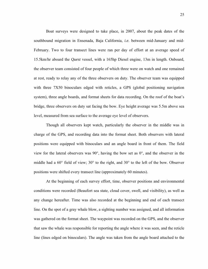
25
Boat surveys were designed to take place, in 2007, about the peak dates of the
southbound migration in Ensenada, Baja California, i.e. between mid-January and mid-
February. Two to four transect lines were ran per day of effort at an average speed of
15.5km/hr aboard the Quest vessel, with a 165hp Diesel engine, 13m in length. Onboard,
the observer team consisted of four people of which three were on watch and one remained
at rest, ready to relay any of the three observers on duty. The observer team was equipped
with three 7X50 binoculars edged with reticles, a GPS (global positioning navigation
system), three angle boards, and format sheets for data recording. On the roof of the boat’s
bridge, three observers on duty sat facing the bow. Eye height average was 5.5m above sea
level, measured from sea surface to the average eye level of observers.
Though all observers kept watch, particularly the observer in the middle was in
charge of the GPS, and recording data into the format sheet. Both observers with lateral
positions were equipped with binoculars and an angle board in front of them. The field
view for the lateral observers was 90°, having the bow set as 0°, and the observer in the
iddle had a 60° field of view; 30° to the right, and 30° to the left of the bow. Observer
ositions were shifted every transect line (approximately 60 minutes).
At the beginning of each survey effort, time, observer positions and environmental
onditions were recorded (Beaufort sea state, cloud cover, swell, and visibility), as well as
ny change hereafter. Time was also recorded at the beginning and end of each transect
ghting number was assigned, and all information
at sheet. The waypoint was recorded on the GPS, and the observer
that saw the whale was responsible for reporting the angle where it was seen, and the reticle
line (lines edged on binoculars). The angle was taken from the angle board attached to the
m
p
c
a
line. On the spot of a gray whale blow, a si
was gathered on the form

26
floor, therefore sightings could only be spotted within a 0-90° angle view, being 90°
irectly aside of the lateral position. The reticle line was defined after setting the first line
n the horizon and the line taken was read from that line down to the last one set over the
able I.
Table I. Reticle distance values used in this study after Kinzey and Gerodette (2001). Tabla I. Valores de la distancia de las retículas utilizados en este estudio de acuerdo a
Kinzey y Gerrodette (2001).
7X50 Binoculars
d
o
sea surface level of the whale blow (sighting). Distance values for each reticle line are
taken from Kinzey and Gerrodette (2001) and the values used in this study are shown on
T
Reticle km 0 8.37 1 0.90 2 0.50 3 0.35 4 0.26 5 0.21 6 0.18 7 0.16 8 0.14 9 0.12 10 0.11 11 0.10 12 0.09 13 0.09 14 0.08

27
The da
II.3. Analytical methods
Ensenada. Analyses
here w
ta entries reported when a marine mammal was sighted were: time, waypoint,
environmental conditions, species, number of individuals, reticle line, angle where it was
sighted, navigation bearing, and comments (e.g. unusual behavior). It is relevant to say that
double counts were not a factor to take care of since the boat traveled at a very slow speed
and sufficient time elapsed between transect lines. Besides, we navigated the lines in a
south-north direction, therefore whales counted in a previously ran southern line would
have passed by the time we ran the next line.
Early abundance analyses (Reilly et al., 1980, 1981) have been modified through
time with the introduction of new mathematical procedures. Recent methods developed by
Buckland et al. (1993), Hobbs et al. (2004), and Rugh et al. (2005) were followed for the
abundance analyses in this work.
Data from three consecutive seasons of shore-based surveys (2003-04, 2004-05, and 2005-
06) were analyzed to estimate the eastern Pacific gray whale stock in
ere split into two sections: first, a description of the migration timing for 2003
through 2006, and secondly, abundance estimation for the respective years.
II.3a. Migration timing
It is well known, beforehand, that the gray whale migration has two main periods; a
southbound migration, which comprises the time the population takes to travel to its
28
reproduction sites, and a northbound migration comprising the time it takes to travel to the
feeding areas. Though in all, each survey season lasted from 9 December through mid-
May, two weeks after the last gray whale sighting, the time span analyzed depended on the
analysis, survey season, and the direction of the migration. Data were therefore split
according to the corresponding period, eliminating from the analysis sightings that were far
from those time intervals. Further, data for the northbound migration were divided into two
hases, separating the migration of whales without calves and that with only cow/calf pairs.
is relevant to mention that northbound migration data were treated separately from those
igratory rate. Migration rate was described with a relative abundance index (number of
whales counted per time effort) to det the beginning, peak and end of both
southbound and northbound migration periods (Rugh et al., 2001). All sightings were
arranged into number of whales per day and er of whales per hour, henceforth a
calculation of the cumulative percentage of sightings per time effort was obtained. The
onset of the migration was considered to be e when 10% of the sightings were
reported, according to the respective onshore survey season. For this study, the peak date is
taken as a median date (when 50% of the sigh at Costa Azul in a
survey season) and the end of the migration is th when 90% of the sightings had been
recorded.
p
It
of the southbound migration, and were used here solely for migration timing analyses.
As a migratory species, evaluation for gray whale abundance includes a description of its
m
ermine
numb
the tim
tings had been obtained
e date
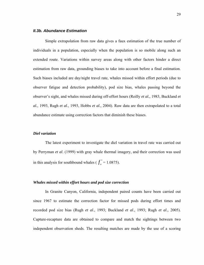
29
II.3b. Abundance Estimation
Simple extrapolation from raw data gives a faux estimation of the true number of
individuals in a population, especially when the population is so mobile along such an
extended route. Variations within survey areas along with other factors hinder a direct
estimation from raw data, grounding biases to take into account before a final estimation.
Such biases included are day/night travel rate, whales missed within effort periods (due to
observer fatigue and detection probability), pod size bias, whales passing beyond the
observer’s sight, and whales missed during off-effort hours (Reilly et al., 1983, Buckland et
et al., 2004). Raw data are then extrapolated to a total
abundance estimate using correction factors that diminish these biases.
Diel variation
The latest experiment to investigate the diel variation in travel rate was carried out
by Perryman et al. (1999) with gray whale thermal imagery, and their correction was used
in this analysis for southbound whales ( = 1.0875).
In Granite Canyon, California, independent paired counts have been carried out
since 1967 to estimate the correction factor for missed pods during effort times and
ugh et al., 1993; Buckland et al., 1993; Rugh et al., 2005).
Captur
al., 1993, Rugh et al., 1993, Hobbs
*n
Whales missed within effort hours and pod size correction
f
recorded pod size bias (R
e-recapture data are obtained to compare and match the sightings between two
independent observation sheds. The resulting matches are made by the use of a scoring
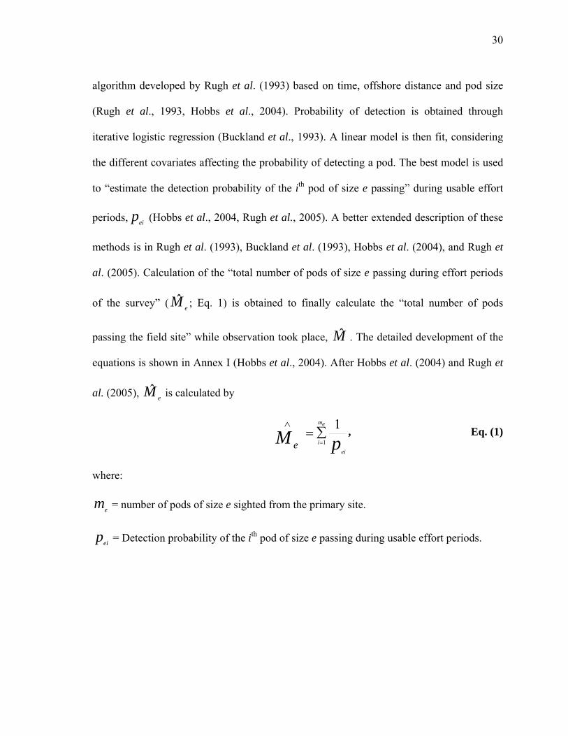
30
algorithm developed by Rugh et al. (1993) based on time, offshore distance and pod size
(Rugh et al., 1993, Hobbs et al., 2004). Probability of detection is obtained through
iterative logistic regression (Buckland et al., 1993). A linear model is then fit, considering
the different covariates affecting the probability of detecting a pod. The best model is used
to “estimate the detection probability of the ith pod of size e passing” during usable effort
periods, eip (Hobbs et al., 2004, Rugh et al., 2005). A better extended description of these
methods is in Rugh et al. (1993), Buckland et al. (1993), Hobbs et al. (2004), and Rugh et
al. (2005). Calculation of the “total number of pods of size e passing during effort periods
of the survey” ( e
passing the field site” while observation took place,
M ; Eq. 1) is obtained to finally calculate the “total number of pods
M . The detailed development of the
equations is shown in Annex I (Hobbs et al., 2004). After Hobbs et al. (2004) and Rugh et
al. (2005), eM is calculated by
pMei
em
ie
11=
∧
where:
m = number of pods of size e sighted from the primary site.
ei = Detection probability of the i pod of size e passing during usable effort periods.
∑= , Eq. (1)
th
e
p

31
M is needed to estimate eW (Eq. 2), the total number of whales passing the site during
effort p
= estimated additive bias correction for e from Laake et al. (1994).
efore this, a correction for bias in estimated pod size needs to be computed, to correct the
stimation of pod size occurs.
Ensenada, paired counts were not made in these years of censuses for the southbound
migration. Nevertheless, it is absolutely fundamental to include these corrections in the
whale’s abundance estimate. In order to account for this inconvenient lack of information,
the correction estimates for pod size bias and whales passing the site within usable effort
hours obtained at Granite Canyon (Rugh et al., 2005) were used for this analysis.
Distance offshore
Before this study, no research on how far whales were migrating from Costa Azul
was undertaken. Depending on the research area, one of the factors that may strongly affect
eriods represented by pods of size e, and it is calculated by Hobbs et al. (2004) and
Rugh et al. (2005) as
( )eee beMW += ˆ , Eq. (2)
where:
W = Total number of whales passing the site during effort periods by pods of size e,
e
∧
e
b
B
fact that undere
Because the counts for this study were initially made with a different objective
(theodolite tracking) and having that it was the first time ever making these counts in
32
the estimated number of gray whales is lacking the awareness of the whale’s migratory
corridor width; that is, distance from shore. Although this species is well known for being a
coastal traveler, a percentage of whales is still being missed because of a limited field of
view. Abundance may be under- or overestimated if the migration corridor is unknown and
distance is not taken into account. Distance from shore of gray whale sightings was
calculated from both boat and onshore surveys to correct for this inconvenience.
Onshore theodolite tracking
Onshore surveys provided data to scrutinize the observer’s viewing capacity.
impossible to track all whales seen with the theodolite, for sometimes more than 3 pods
were sighted at the same time, and only one could be followed. However, it was intended to
get as many paths as possible.
Information consisted in gray whale paths, which were gathered from theodolite tracking.
Methods for theodolite tracking are explained in the above section. It was practically
The theodolite gives out two angles; the vertical angle and the azimuth, which is the
horizontal angle from the true northern orientation. These angles were transferred to
T-Track (Cipriano, 1980), which gave northing and easting positions (in relative
meter units). W
computed, but for the interest of this study, the distance of the given geographic position
from
ith AUTOCAD computer program. A standard line was drawn parallel to the coast, and
distance perpendicular to the coastline, where the survey site was located, to the whale
migration paths was measured (Figure 3).
program
ith this information, the exact geographic position of the whale can be
the survey site is most relevant. Paths were drawn, based on the geographical points,
w
33
Once all measurem ts were done, analytical measures followed. For the first
survey season, all sightings that were more than 7km away were excluded from analyses,
since it was the first season and m
en
isidentification was most probable, as was learned from
later experience. Also, transects not falling within the southbound migration period were
were arranged in different categorical bins, depending on comparisons. In
order to compare to Shelden and Laake’s 2002 article, bins of precisely 1.3705km (0.74nm)
distance intervals up to 40km (21.6 n.m.) from shore were also analyzed. Chi-square tests
were run to test for significant differences
ontingency tables were made to test independence of distance from shore among the
s for all three observation years.
not included in this analysis.
Distances
at a 95% level among distance intervals and also
c
surveyed years (Spatz and Johston, 1989), in order to assess if it was correct to apply the
same correction factor to abundance estimate

34
Figure 3. Map showing gray whale tracking lines taken from the theodolite from
conteos desde tierra.
nt to mention that waypoints not falling within
the strip width (1km) were excluded from the analyses. Also, to avoid taking data not
surveys.
Figura 3. Mapa con las trayectorias de ballena gris tomadas con el teodolito de los
Boat surveys
Data obtained from the boat transects were analyzed in a similar way as the shore-
based theodolite tracking. Waypoints were set on a map and distance was measured from
the coastline to the waypoint. It is importa

35
falling
o distance bins, to find the gray whale’s migration corridor.
Chi-squ
ly limited or
conditioned by climate variations. Effort was usually partially canceled when Beaufort 3
sea state was present, rain came along, or fog was too dense, and it was resumed when
these conditions improved. In the worst of cases, that is, if these conditions remained
unfavorable for two hours, effort for that day was canceled. Also, recalling the field
methods, count surveys for the southbound migration took place three days per week rather
than all seven days; therefore, there are days on which no surveys were undertaken. Adding
to these missing data, count surveys only took place during the day, from 0700-1400h
leaving empty counts any time before and after each survey (nocturnal hours are included
in this missing time of effort). According to Buckland (1992) and Breiwick (pers. comm. 2),
within the strip width and for better confidence, sightings that were recorded with
reticle line zero or 0.5 were removed from final analyses. Once this distance was obtained,
and with the angles reported from the angle boards, basic trigonometric computations
provided a true distance of the sighting from shore.
These data were arranged int
are tests of independence followed to find yearly and inter-bin significant
differences. After comparing sightings from theodolite tracking and from boat surveys the
percent of sightings missed from the shore station because of distance was estimated.
Missed whales during off-effort hours (ft)
Twenty-four daily hours of counts are impossible due to variable reasons. Weather
conditions are not constant throughout the day and effort time was usual
2 National Marine Mammal Laboratory, Alaska Fisheries Science Center, NMFS, NOAA, 7600 Sand Point Way NE, Seattle, Washington 98115 USA.
36
the performed effort time is categorized or grouped into time interval data sets. The
resulting count periods, with gaps in between (periods in which no effort or counts were
performed), are then frequency counts of whales passing the survey area within that time
interval. These frequency counts form the basis for the analysis to correct for missed counts
during off-effort hours.
Code design for time intervals
Since count periods are needed to follow on with the use of the FORTRAN
Gwnormf77 program (Breiwick, pers. comm.) for the computation of (pods missed
during off-effort periods), they should be categorized in a systematic manner in order to
have reasonable results. It is true that if a single visibility code contemplating the
environmental conditions (sea state, cloud cover, fog, among others) is assigned the
moment the sighting was recorded; these count periods can easily be grouped. Single code
assignment (contemplating these factors as a whole) on the spot of a pod, was not done for
e surveys analyzed in this study. This study used a different method developed from the
a change occurred. Since environmental conditions do not vary
y, a sighting may have been done at the time all environmental conditions
change
tf
th
recorded data to generate the count periods needed. Environmental conditions were
recorded individually, rather than into a single code, from the beginning of a day’s effort
nd anytime hencefortha
simultaneousl
d, or, with change in at least one of these factors. Consequently, categorization of
time intervals would be difficult due to the many resulting data groups. To discard the
many possible groups, a code design was developed to group the counts into proper time
37
intervals. The general visibility code was designed, based on a frequency criterion.
Frequencies were based on number of sightings per environmental condition.
There were three obvious possibilities in viewing conditions according to the
environmental factors recorded: best, acceptable and worst (Table II). The best of
Each
f the categorized conditions (best, acceptable and worst) was then subcategorized into
e resulting frequencies. Codes (1-3) were then
assigne
conditions was a day with a clear sky, no fog nor swell and sea state under Beaufort one.
The worst possible working conditions are shown in Table II. Data was arranged into
frequency counts according to each of the four recorded environmental condition. These
percentages gave an idea of how each condition influenced on the sighting of a pod.
o
specific environmental conditions, given th
d to each of these categorized conditions according to the required subcategorized
environmental factors (see Table III). Hence, a pod could be single-coded according to the
environmental factors under which it was recorded. For example, a sighting with a “best
categorized condition” had to occur under Beaufort 1, visibility within a range of 31 to 50
km, and 40% or less cloud cover in order to yield code 1. Presence of swell was
independent since 95% of sightings were recorded under this condition (see percentages in
Table III). The codes were used to set the time intervals at which pods were sighted under
alike environmental conditions.
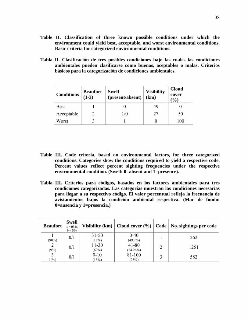
38
Table II. Classification of three known possible conditions under which the
Basic criteria for categorized environmental conditions.
Tabla II. Clasificación de tres posibles condiciones bajo las cuales las condiciones
básicos para la categorización de condiciones ambientales.
environment could yield best, acceptable, and worst environmental conditions.
ambientales pueden clasificarse como buenas, aceptables o malas. Criterios
0 = 5%
Table III. Code criteria, based on environmental factors, for three categorized conditions. Categories show the conditions required to yield a respective code. Percent values reflect percent sighting frequencies under the respective environmental condition. (Swell: 0=absent and 1=presence).
Tabla III. Criterios para códigos, basados en los factores ambientales para tres
condiciones categorizadas. Las categorías muestran las condiciones necesarias para llegar a su respectivo código. El valor porcentual refleja la frecuencia de avistamientos bajos la condición ambiental respectiva. (Mar de fondo: 0=ausencia y 1=presencia.)
Beaufort Swell 1 = 95% Visibility (km) Cloud cover (%) Code No. sightings per code
1 (90%) 0/1 31-50
(18%) 0-40
(49.7%) 1 262 2
(9%) 0/1 11-30 (69%)
41-80 (24.26%) 2 1251
3 1(%) 0/1 0-10
(13%) 81-100
(25%) 3 582
Conditions Beaufort Swell (present/absent)
Visibility (km)
Cloud cover (%)
(1-3)
Best 1 0 49 0 Acceptable 2 1/0 27 50 Worst 3 1 0 100
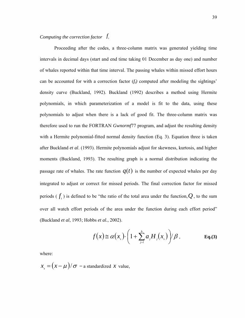
39
Computing the correction factor
Proceeding after the codes, a three-column matrix was generated
tf
yielding time
intervals in decimal days (start and end time taking 01 December as day one) and number
of whales reported within that time interval. The passing whales within missed effort hours
can be accounted for with a correction factor (ft) computed after modeling the sightings’
density curve (Buckland, 1992). Buckland (1992) describes a method using Hermite
polynomials, in which parameterization of a model is fit to the data, using these
polynomials to adjust when there is a lack of good fit. The three-column matrix was
therefore used to run the FORTRAN Gwnormf77 program, and adjust the resulting density
with a Hermite polynomial-fitted normal density function (Eq. 3). Equation three is taken
after Buckland et al. (1993). Hermite polynomials adjust for skewness, kurtosis, and higher
moments (Buckland, 1993). The resulting graph is a normal distribution indicating the
passage rate of whales. The rate function )(tq is the number of expected whales per day
integrated to adjust or correct for missed periods. The final correction factor for missed
periods ( f ) is defined to be “the ratio of the total area under the function,Q , to the sum t
over all watch effort periods of the area under the function during each effort period”
(Buckland et al, 1993; Hobbs et al., 2002).
( ) ( ) ( ) βα /11
⎟⎠⎞
⎜⎝⎛ +⋅≅ ∑
=
b
jsjjs xHaxxf , Eq.(3)
where:
( ) σµ /−=xs = a standardized x value, x
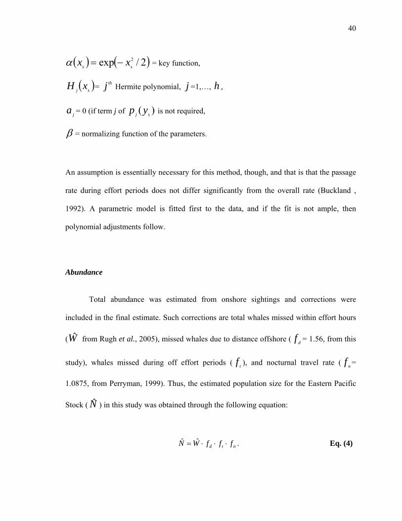
40
( ) ( )2/exp 2ss xx −=α = key function,
) thj j h( sj
(if term j of )( sj yp is not required,
x = Hermite polynomial, =1,…, ,
j
H
a = 0
β = normalizing function of the parameters.
assu n is essentia method, though, and that is that the passage
te dur eriods oes not diffe the overall rate (Buckland ,
992). A parametric model is fitted first to the data, and if the fit is not ample, then
ial adjustments follow.
Abund
include
(W from df = 1.56, from this
study), whales mi ring off effort periods ( f nd nocturnal travel ra nf =
1.0875, from Perrym a n size fo Eas c
An mptio lly necessary for this
ra ing effort p d r ignificantly from s
1
polynom
ance
Total abundance was estimated from onshore sightings and corrections were
d in the final estimate. Such corrections are total whales missed within effort hours
Rugh et al., 2005), missed whales due to distance offshore (
ssed du t ), a
ted populatio
te (
tern Pacifian, 1999). Thus, the estim r the
Stock ( N ) in this s was obta ough the f g equatio
td ffW ⋅⋅⋅ˆ
tudy ined thr ollowin n:
N =ˆnf . Eq. (4)
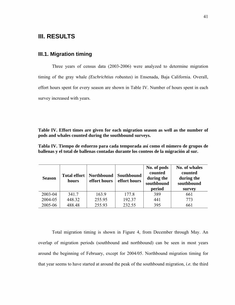
41
III. RESULTS
I.1. Migration timing
(2003-2006) were analyzed to determine migration
timing
Total effort Northbound Southbound
II
Three years of census data
of the gray whale (Eschrichtius robustus) in Ensenada, Baja California. Overall,
effort hours spent for every season are shown in Table IV. Number of hours spent in each
survey increased with years.
Table IV. Effort times are given for each migration season as well as the number of pods and whales counted during the southbound surveys. Tabla IV. Tiempo de esfuerzo para cada temporada así como el número de grupos de ballenas y el total de ballenas contadas durante los conteos de la migración al sur.
Season hours effort hours effort hours
No. of pods counted
during the southbound
period
No. of whales counted
during the southbound
survey 2003-04 341.7 163.9 77.8 389 661 12004-05 448.32 255.95 192.37 441 773 2005-06 488.48 255.93 232.55 395 661
nd northbound) can be seen in most years
around the beginning of February, except for 2004/05. Northbound m
that year seems to have started at around the peak of the southbound migration, i.e. the third
Total migration timing is shown in Figure 4, from December through May. An
overlap of migration periods (southbound a
igration timing for
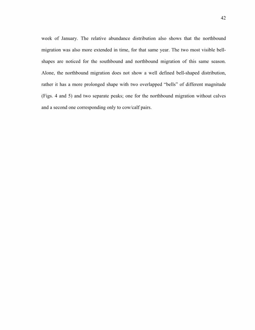
42
week of January. The relative abundance distribution also shows that the northbound
migration was also that same year. The two most visible bell-
shapes are noticed for the southbound and northbound migration of this same season.
Alone, the northbound migration does not show a well defined bell-shaped distribution,
rather it a agnitude
(Fi two sep for the northbound migration without calves
and a second one corresponding only to cow/calf pairs.
more extended in time, for
has more prolonged shape with two overlapped “bells” of different m
gs. 4 and 5) and arate peaks; one
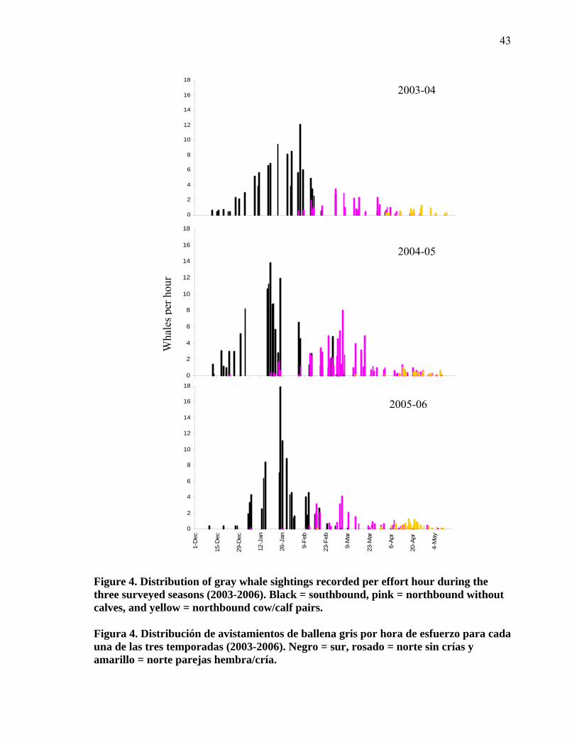
43
Figure 4. Distribution of gray whale sightings recorded per effort hour during the three surveyed seasons (2003-2006). Black = southbound, pink = northbound without calves, and yellow = northbound cow/calf pairs. Figura 4. Distribución de avistamientos de ballena gris por hora de esfuerzo para cada una de las tres temporadas (2003-2006). Negro = sur, rosado = norte sin crías y amarillo = norte parejas hembra/cría.
Wha
les p
er h
our
0
4
10
12
14
16
18
2
6
8
0
2
4
6
10
16
8
12
14
18
0
6
8
c
15-D
ec n
26-J
an
9-Fe
b b
9-M
ar
23-M
ar
20-A
pr
4-M
ay
2
4
10
12
14
16
18
1-D
e
29-D
ec
12-J
a
23-F
e
6-Ap
r
2003-04
2004-05
2005-06
44
Figure 5. Distribution of northbound migrating whales sighted per hour of effort during the three surveyed seasons (2003-2006), including cow/calf pairs. a) Whales without calves, b) cow/calf pairs. Figura 5. Distribución del número de ballenas registradas por hora de esfuerzo en la migración al norte durante las tres temporadas de muestreo (2003-2006). a) Ballenas sin crías, b) parejas madre/cría.
0
0.5
1
1.5
2
0
0.5
1
1.5
2
0
0.5
1
1.5
10-M
ar
17-M
ar
24-M
ar
31-M
ar
7-Ap
r
14-A
pr
21-A
pr
28-A
pr
5-M
ay
12-M
ay
2
0
2
4
5
6
7
9
1
3
8
0
2
3
4
5
7
9
1
6
8
0
1
2
3
4
5
6
7
8
15-J
an
29-J
an
12-F
eb
26-F
eb
12-M
ar
26-M
ar
9-A
pr
23-A
pr
7-M
ay
9
Re
vend
ceal
r)la
tiab
uan
(wh
es/h
a b2003-04
2004-05
2005-06
45
III.1a. Southbound migration timing
ata analyzed for the southbound migration were taken from resulting survey
information obtained from 9 December through 15 March in order to make annual
comp e
pent for the 2003-04 southbound season (Table IV). An increase in number of whales (773
hales; 441 pods) was observed for 2004/05, yet for the following year this number
ecreased to a similar number of whales as seen in the first survey year. However, effort
me was also increased from the first survey year to the last and considering this, fewer
hales were seen (661) for the 2005-06 southbound survey, regardless of the increase in
umber of observation hours (232.55h) (Table IV).
The relative abundance of southbound grays is depicted in Figure 6 as number of
bserved whales per hour during a two-month period. It reflects the passage rate of whales,
ith a bell-sh distribution, during effort hours. From this rate, the timing at which a
ercent of the ulation is passing Ensenada can be estimated. Timing for the southbound
bundance dis tion in this study was from December to early March in every survey
eason (Fi ). The bell-shaped graphs reflect the gray’s southbound migration passage
te as an initial flux (the onset of whales passing Ensenada), rising to a peak, and then
moothly declining, marking the end. The end is assumed to be when most whales have
aveled south past Ensenada, and the southbound migration there is considered to be over.
he tails of the migration in Ensenada are shown on Table V.
D
arisons. A total of 661 whales were seen (389 pods) during 177.8 hours of effort tim
s
w
d
ti
w
n
o
w aped
pop
tribu
p
a
s g. 6
ra
s
tr
T

46
0
14
16
18
2
4
6
8
10
12
0
2
4
6
8
10
12
14
16
18
0
2
4
6
8
10
12
14
16
18
1-D
ec
15-D
ec
29-D
ec
12-J
an
26-J
an
9-Fe
b
23-F
eb
9-M
ar
Figure 6. Distribution of southbound gray whales sighted per effort hour during the three surveyed seasons. Time is shown from 01-Dec. to 15-Mar. Figura 6. Distribución de avistamientos de ballena gris por hora de esfuerzo en la migración al sur para las tres temporadas de muestreo, del 1 de diciembre al 15 de marzo.
Rel
ativ
e ab
u
ndan
ce (w
hale
s/hr
)
2005-06
2004-05
2003-04

47
Table V. Dates of occurrence of the tails of the southbound migration and median dates (50%) taken from the relative abundance index, for each migration season.
abla V. Fechas de las proporciones extremas (10% y 90%) de la migración al sur y índice de abundancia relativa para cada
mporada.
Season 10% 50% 90%
Tfechas medianas (50%), tomadas del te
2003/04 02 January 23-29 January 13 February 2004/05 25 December 17-18 January 13 February 2005/06 06 January 25 January 12 February
There seem
migration season, tim
s to be a head-start of about a week or two in the onset of the 2004/05 (Dec. 25)
e at which 10% of the sightings had been recorded. This early arrival
also seen for the median dates on that same year (17-18 January), notwithstanding the
ates obtained for the other two years, which are in late January. However, the end of the
igration fell on the same day (12-13 February) for all three years. After averaging the
lative abundance for the southbound migration (table at counts did not
able VI. Mean relative abundance index showing whales per hour during the three igration seasons (2003-2006).
abla VI. Índice promedio de abundancia relativa mostrando numero de ballenas por ora durante las tres temporadas de migración (2003-2006).
Mean southbound Mean northbound Mean northbound
is
d
m
re VI), it is noted th
Tm Th
whales/day whales/hr whales/day whales/hr CC/day CC/hr2003/04 24.59 3.97 4.78 1.03 1.28 0.43 2004/05 23.42 3.87 8.94 1.53 1.37 0.19 2005/06 22.79 3.56 3.71 0.62 1.59 0.26
48
rise in 2004-05. Therefore, it cannot be said that whales were passing at a faster rate than
date with maximum rate of whales per hour) coincides
e
re noticeable in 2004-2005 (Fig. 6) where a week-delay
was observed.
III.1b. Northbound migration timing
The northbound migration has a different behavior from the southbound migration;
therefore, it is treated separately. Migration in the northbound direction is divided into two
sets of migrants; migration without calves and migration with only cow/calf pairs. Whales
falling within the first northbound migrating group are early pregnant females, adult males,
mestrous, anestrous and immature females, and immature males (Rice and Wolman, 1971).
Behavior for this data shall be described first.
The period for the northbound migration without calves took place from early
February to early April (Figs. 4 and 5a). The beginning for the migration without calves
was not variable for the first two seasons; dates coincided early in 12-13 February (Table
VII). A later date in mid- February is reported for the onset of the 2005-06 northbound flux.
Consistency in median dates is shown for 2004-05 and 2005-06; sightings for those two
years fell within the same median date, 04 March. The same pattern in date consistency is
obtained for the end of the migration, where 90% of the sightings are reported between 9-
10 April. In fact, despite that counts were higher in 2004/05 (1.53 whales/hr; table VI),
migration timing for this period was also longer. During the last survey season, a delay in
usual and hence the early arrival.
The peak of the migration (
with the median date for every respective year. Even though the peak date is seen to hav
varied in all three years, it was mo
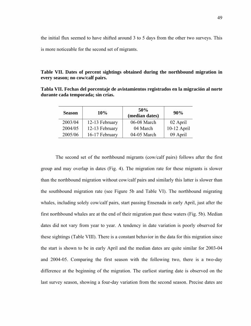
49
the initial flux seemed to have shifted around 3 to 5 days from the other two surveys. This
is more
every season; no cow/calf pairs.
Tabla VII. Fechas del porcentaje de avistamientos registrados en la migración al norte
The second set of the northbound migrants (cow/calf pairs) follows after the first
group and may overlap in dates (Fig. 4). The migration rate for these migrants is slower
than the northbound migration without cow/calf pairs and similarly this latter is slower than
the southbound migration rate (see Figure 5b and Table VI). The northbound migrating
whales, including solely cow/calf pairs, start passing Ensenada in early April, just after the
first northbound whales are at the end of their migration past these waters (Fig. 5b). Median
dates did not vary from year to year. A tendency in date variation is poorly observed for
these sightings (Table VIII). There is a constant behavior in the data for this migration since
the start is shown to be in early April and the median dates are quite similar for 2003-04
and 2004-05. Comparing the first season with the following two, there is a two-day
difference at the beginning of the migration. The earliest starting date is observed on the
last survey season, showing a four-day variation from the second season. Precise dates are
Season 10% 90%
noticeable for the second set of migrants.
Table VII. Dates of percent sightings obtained during the northbound migration in
durante cada temporada; sin crías.
50% (median dates)
2003/04 12-13 February 06-08 March 02 April 2004/05 12-13 February 04 March 10-12 April 2005/06 16-17 February 04-05 March 09 April
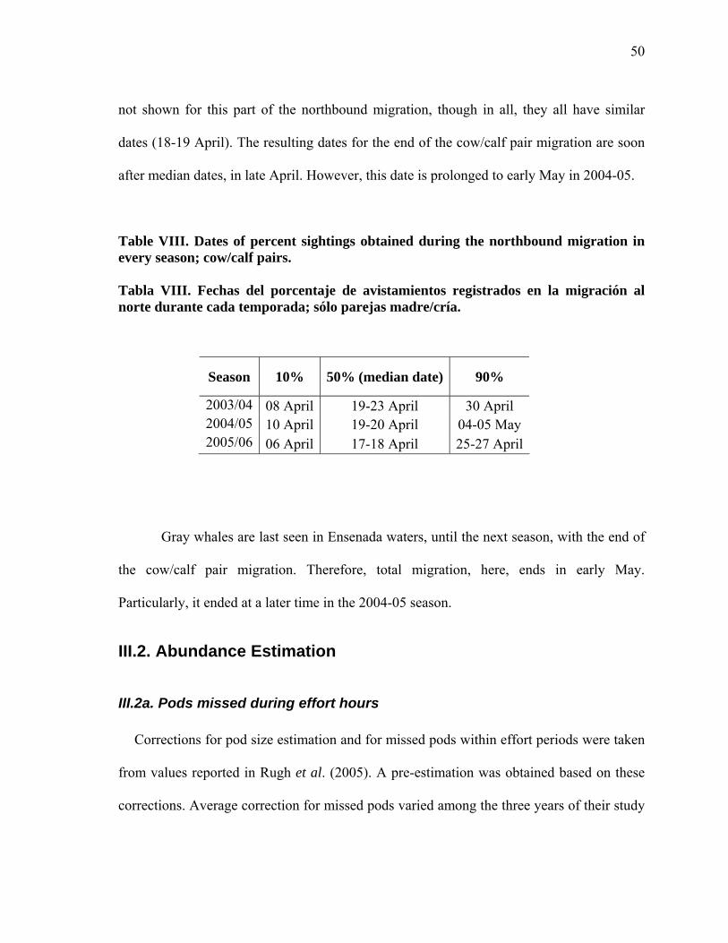
50
ot shown for th ilar
ates (18-19 April). The resulting dates for the end of the cow/calf pair migration are soon
fter median dates, in late April. However, this date is prolonged to early May in 20
able V Dates of percent sightings obtained during the northbound migration in very se ; cow/calf pairs.
abla V Fechas del porcentaje de avistamientos registrados en la migración al orte du te cada temporada; sólo parejas madre/cría.
Gray whales are last seen in Ensenada waters, until the next season, with the
e cow/calf pair migration. Therefore, total migration, here, ends in early May.
Particularly, it ended at a later time in the 2004-05 season.
I.2. Abundance Estimation
corrections. Average correction for missed pods varied among the three years of their study
Season 10% 50% (median date) 90%
n is part of the northbound migration, though in all, they all have sim
d
a 04-05.
T III.
ason
III.ran
e Tn
2003/04 08 April 19-23 April 30 April 2004/05 10 April 19-20 April 04-05 May 2005/06 06 April 17-18 April 25-27 April
end of
th
II
III.2a. Pods missed during effort hours
Corrections for pod size estimation and for missed pods within effort periods were taken
from values reported in Rugh et al. (2005). A pre-estimation was obtained based on these

51
(1997-98, 2000-01 and 2001-02). Therefore, the estimation of whales passing the survey
site ( e ) is calculated using the mean of the correction estimated for the last two years in
Rugh et al. (2005) for each survey season analyzed in this study (Table IX).
W
Table IX. Estima f g ite (W ), in each surveyed seaso for s w eriods and pod size bias due to observers as reported in Rugh et al. (2005). eW = No. whales in pods of size e.
Psi
Average
2003-04 2004-05 2005-06
tion of total number o whales passin the survey sn, using corrections missed pod ithin effort p
Tabla IX. Estimación del total de ballenas que pasaron el sitio de observación (W ), en cada temporada, utilizando las correcciones para grupos no observados dentro de horas de esfuerzo y sesgo de los observadores por tamaño de grupo, tal como lo reportan Rugh et al. (2005). eW = No. ballenas en grupos de tamaño e.
od ze
Correction for missed
pods
Bias-correctedpod size
No. of pods
eW No. of pods
eW No. of pods
eW
1 1.28 1.94 203 504.35 237 588.82 238 591.31 2 1.229 2.65 114 370.72 120 390.23 102 331.70 3 1.156 3.61 55 229.33 51 212.65 26 108.41 4 1.1015 4.25 10 46.81 21 98.31 12 56.18
5 1.0525 5.25 1 5.53 8 44.21 8 44.20
6 1.043 5.25 2 10.95 2 13.04 3 16.43 7 1.0285 7.25 - - 1 7.46 1 7.46 8 1.028 8.25 1 8.48 2 16.96
All 1.25 2.43 386 440 392
W 6 ˆ 1,176.2 1,354.7 1,172.
ectio in this y’s fina ation a latest r ed cor n
estim et al., 2005). The pre-estimations for our study were
The corr ns used stud l estim re the eport rectio
ates (2000-01 and 2001-02; Rugh
52
1,176, 1,355 and 1,173 individuals for the respective 2003/04, 2004/05 and 2005/06 survey
season results. An early tendency can be seen as an increase of individuals in 2004/05 and
then a d
III.2b. Pods missed due to distance from shore
olite tracking
For the 2003/04 survey, a total of 49 sightings were tracked
were tracked in 2004/05 and during the last
gathered. Sightings were categorized into distance interval bins of 1.375km
to 0.74nm (Table X). Table X shows percent of sightings observed per distance in
every year as well as the respective chi-square value to test for differences in ance
intervals (each bin represents a distance interval).
Distance intervals are rounded to two digits after the decim l point, though this was
only done to ease the view and reading of graphic and table results. In analyses, this
numbers were used to the precision of 0.74 nautical miles. There was a statistically
significant difference in the number of sightings among bins in each of the three seasons
(2003-2004: χ2 = 32.74, 2004-2005: χ2 = 43.95, 2005, 2006: χ2 = 81.66; df=4, p<0.001).
ecrease in 2005/06 similar to estimates calculated in 2003/04.
Onshore theod
with the theodolite, 39
survey season (2005/06), 58 tracks were
, the equivalent
terval for
dist
a
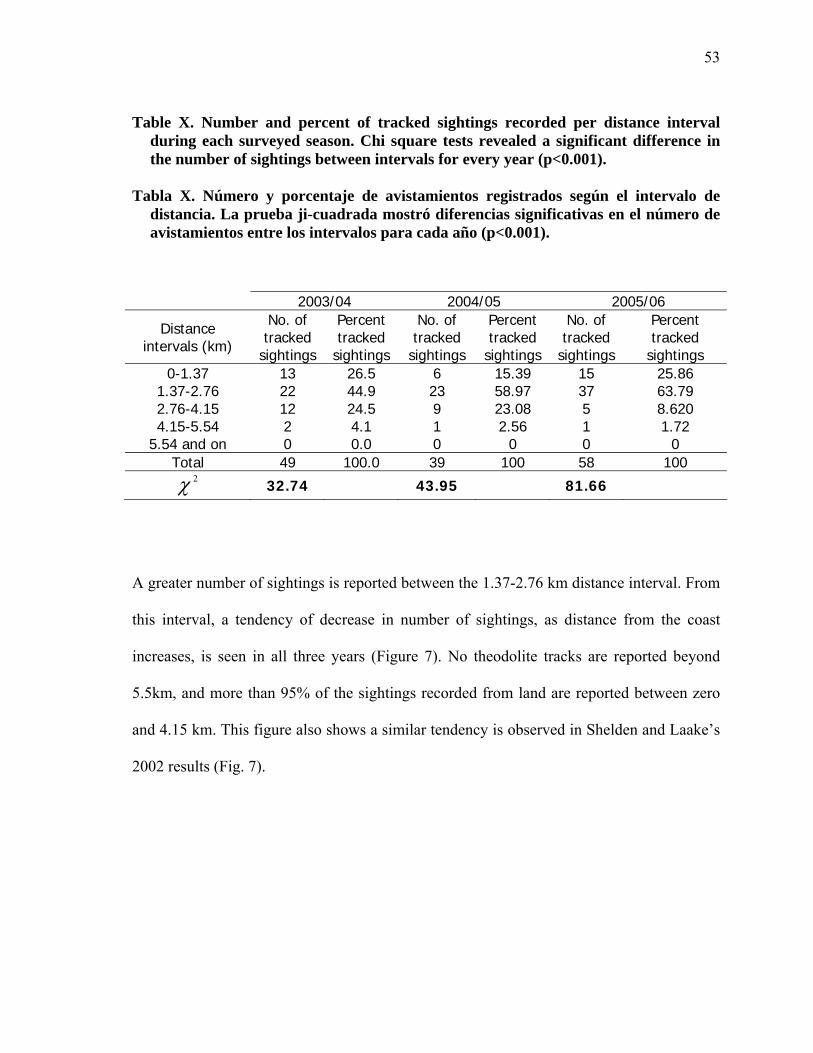
53
Table X. Number and percent of tracked sightings recorded per distance interval
the number of sightings between intervals forduring each surveyed season. Chi square tests revealed a significant difference in
every year (p<0.001). Tabla X. Número y porcentaje de avistamientos registrados según el intervalo de
distancia. La prueba ji-cuadrada mostró diferencias significativas en el número de avistamientos entre los intervalos para cada año (p<0.001).
2003/04 2004/05 2005/06
Distance intervals (km) tracked
sightingstracked
tings
No. of tracked
sightin
Percent tracked ghtings
No. of tracked
Percent tracked
sightings
No. of Percent
A greater number of sightings is reported between the 1.37-2.76 km distance interval. From
this interval, a tendency of decrease in number of sightings, as distance from the coast
increases, is seen in all three years (Figure 7). No theodolite tracks are reported beyond
5.5km, and more than 95% of the sightings recorded from land are reported between zero
and 4.15 km. This figure also shows a similar tendency is observed in Shelden and Laake’s
2002 results (Fig. 7).
sigh gs si sightings 0-1.37 13 6.5 9 25.86 2 6 15.3 15
1.37-2 97 63.79 2.76-4 .08 8.620 4.15-5 6 1.72
5.54 and 0 Total 49 100.0 39 100 58 100
.76 22 44.9 23 58.3
37 .15 12 24.5 9 2 5 .54 on
2 4.1 0 0.0
1 2.50 0
1 0
2χ 32.74 43.95 81.66
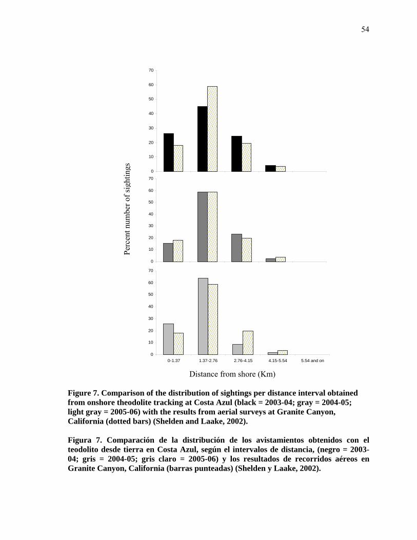
54
Figure 7. Comparison of the distribution of sightings per distance interval obtained zul (black = 2003-04; gray = 2004-05;
light gray = 2005-06) with the results from aerial surveys at Granite Canyon, Ca
Granite Canyon, California (barras punteadas) (Shelden y Laake, 2002).
from onshore theodolite tracking at Costa A
lifornia (dotted bars) (Shelden and Laake, 2002).
Figura 7. Comparación de la distribución de los avistamientos obtenidos con el teodolito desde tierra en Costa Azul, según el intervalos de distancia, (negro = 2003-04; gris = 2004-05; gris claro = 2005-06) y los resultados de recorridos aéreos en
Perc
ent n
umbe
r of s
ight
ings
0
1
2
30
40
50
60
0
0
70
0
30
50
60
70
0-1.37 1.37-2.76 2.76-4.15 4.15-5.54 5.54 and on
10
20
40
0
10
30
40
70
stance from shore (Km)
50
60
20
Di

55
Inter-annual comparisons in data distribution were also tested for independence
among years, resulting in a rejection of the null hypothesis. Hence, the theoretical
assumption was accepted ( 2χ = 8.33, df = 6, n = 146 p>0.001), inferring that the spatial
distribution of gray whales reported from shore did not differ among the three years (2003-
2006). That is, there was no difference in the distribution of percent sightings in the
Bo
an
Su onsequences
f weather variations and limitations. Throughout the entire study period, 118 sightings of
y ght re gathe d, th after dat trea sample
ze red o 78 usab htings.
mamm served d g th veys her ay w es,
ort-b common phin (Delphinus delphis), g-bea omm dol
elph ensis), bottlenose dolphin (Tursiops truncatus), Pacific white-sided dol
ageno hus obliq s), fin whale (Balaenoptera physalus)
(Zalophus californianus. californianus and harbor seal ( ). A
and to a surprise, a gray whale cow/calf pair was sighted at the end of one of the long
transects (40km from shore; 07 February, 2007), though it was not included in the analyses
because it was at a yet further distance and did not fall within the sampling area.
categorical bins among the years analyzed from onshore theodolite tracking.
at surveys
Surveys were done from 22 January to 9 February running a total of 31.5 inshore
d 6 offshore transect lines. On average, three to four transect lines were ran per day.
rvey time extension and number of transects surveyed in a day were both c
o
gra whales (207 gray whales si ed) we re ough a tment,
si uced t le sig
Marine als ob urin ese sur , ot than gr hal were
sh eaked dol lon ked c on phin
(D inus cap phin
(L rhync uiden , California sea lion
), Phoca vitulina richardsi lso,
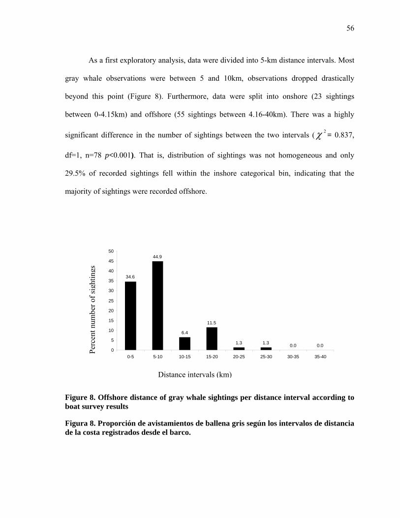
56
As a first exploratory analysis, data were divided into 5-km distance intervals. Most
gray whale observations were between 5 and 10km, observations dropped drastically
beyond this point (Figure 8). Furthermore, data were split into onshore (23 sightings
between 0-4.15km) and offshore (55 sightings between 4.16-40km). There was a highly
significant difference in the number of sightings between the two intervals ( 2χ = 0.837,
s, distribution of sightings was not homogeneous and only
29.5%
Figure 8. Offshore distance of gray whale sightings per distance interval according to boat survey results
Figura 8. Proporción de avistamientos de ballena gris según los intervalos de distancia de la costa registrados desde el barco.
Perc
ent n
umbe
r of s
i
df=1, n=78 p<0.001). That i
of recorded sightings fell within the inshore categorical bin, indicating that the
majority of sightings were recorded offshore.
Distance intervals (km)
44.945
6.4
0.0 0.0
34.6
0
10
20 25 30 35 40
0-5 5-10 10-15 15-20 20-25 30-35 35-40
11.5
1.3 1.35
15
50
25-30
gs
ghtin

57
0
10
0-1.37 1.37-2.76 2.76-4.15 4.15-5.54
20
30
40
50
60 this studySheld nd Laake, 200
dis astline (Fig. 9).
As in Shelden and Laake (2002), inshore data were subcategorized into 1.3705km
tance intervals (the equivalent to their 0.74nm) up to 5.5 km from the co
Inshore sighting distribution rejected homogeneity ( 2χ = 5.76; df=3, n=34 p<0.001). Not
ny sightings were obtained in the first kilometer from shore, yet numm
en a 2
a ber of sightings
increased with distance.
divided into 1.3705km intervals (0.74nm), to compare with results from Shelden and surveys at Granite Canyon, California.
Figura 9. Distribución del porcentaje de avistamientos dentro de los primeros 5.54km de la costa y divididos en intervalos de 1.3705km (0.74nm), para comparar con los resultados de censos aéreos en Granite Canyon, California, por Shelden y Laake (2002).
ghtin
gs
Figure 9. Distribution of percent sightings obtained within 5.54km from shore and
Laake’s (2002) aerial
Perc
ent n
umbe
r of s
i
Distance intervals (km)

58
Comparison of onshore and boat surveys: Correction factor ( df )
shore and offshore distances were initially categorized based on information from
helden and Laake’s (2002) study. Nevertheless, results from onshore distance analyses
heodolite tracking) determined that percent sighting distribution was similar to results
ported in Shelden and Laake’s (2002) study (Figure 8). Observers at Costa Azul recorded
ore than 95% he tracks below 4.15km and no recordings were reported at a further
istance than 5k owever, boat survey results indicated that numerous whales were still
assing beyond distance. Eyesight limitation from shore to sea was then determined to
e at 5.5km for study. Nonetheless onshore and boat surveys together determine true
bserver eyesig om the observation point to be at 4.15 km. For this study, observer
yesight was taken to be the distance where most sightings (>90%) were being recorded by
bservers. Table XI shows the observer viewing limitation when compared to the percent
ightings obtained from boat surveys. A comparison of the 2007 boat survey results with
e three years of shore-based surveys shows the cumulative percent sightings from boat
urveys compared with the cumulative percent sightings obtained with the theodolite from
nd. The cumulative percent comparison was made with results obtained up to 20km since
ere very few sightings recorded beyond this distance (Figure 10).
In
S
(t
re
m of t
m. H
this
this
ht fr
d
p
b
o
e
o
s
th
s
la
th
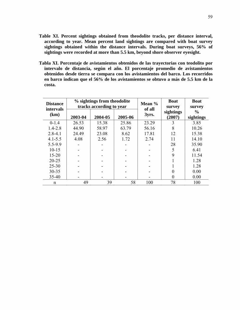
59
Table according to year. Mean percent land sighti ith boat survey
sightings were recorded at more than 5.5 km, beyond shore observer eyesight.
% sightings from theodolite tracks according to year
XI. Percent sightings obtained from theodolite tracks, per distance interval,
sightings obtained within the distance intervals. During boat surveys, 56% of
Tabla XI. Porcentaje de avistamientos obtenidos de las trayectorias con teodolito por
intervalo de distancia, según el año. El porcentaje promedio de avistamientos obtenidos desde tierra se compara con los avistamientos del barco. Los recorridos en barco indican que el 56% de los avistamientos se obtuvo a más de 5.5 km de la costa.
ngs are compared w
Distance
(km) 2003-04 2004-05 2005-06
Mean % of all 3yrs.
Boat survey
sightings (2007)
Boat survey
% sightings
intervals
0-1.4 26.53 15.38 25.86 23.29 3 3.85 1.4-2.8 44.90 58.97 63.79 56.16 8 10.26 2.8-4.1 24.49 23.08 8.62 17.81 12 15.38 4.1-5.5 4.08 2.56 1.72 2.74 11 14.10 5.5-9.9 - - - - 28 35.90 10-15 - - - - 5 6.41 15-20 - - - - 9 11.54 20-25 - - - - 1 1.28 25-30 - - - - 1 1.28 30-35 - - - - 0 0.00 35-40 - - - - 0 0.00
n 49 39 58 100 78 100

60
0
20
40
60
80
100
0-
1.4-
2.8-
4.2-
5.5-
6.9-
8.3-
9.7-
11
11.1
-12
12.5
-13
13.9
-15
15.3
-16
16.7
-18
18.0
-19
19.4
-20
Distanc
umu
ve p
ert s
igin
gs
1.4
2.8
4.2
5.5
6.9
8.3
9.7 .1 .5 .9 .3 .7 .0 .4 .8
e intervals (Km)
Cla
tice
nht
Boat surveys2003-04 Theodolite2004-05 Theodolite2005-06 Theodolite
e obtained from land w n). More than 50% of boat sightings were recorded beyond 5.5km, the distance at which the shore observer is able to record with the
igura . P centaje acu ulado de los avistamientos obtenidos de barco y desde tierra con el teodolito (por temporada). Más del 50% de avistamientos desde barco se egistr a m d 5km, distancia máxima a la que el observador en tierra logra
registrar con el teodolito.
parison of the average percent sightings obtained
nst the percent sightings obtained in all
transec es in 200 at s s. A own able XI, 56% of the sightings are
recorded beyond the shore o ). This can be better portrayed in the
comparison shown in Figure 10. As a result, a single-general correction factor of 1.56 was
in all three years for abundance estimation.
Figure 10. Cumulative percent sightings from boat surveys and thosith the theodolite (per seaso
theodolite.
F 10
an
t lin
or m
r ás e 5.
Nevertheless, Figure 11 shows a com
during the three years of onshore surveys agai
ran the 7 bo urvey s sh in T
bserver eyesight (5.5km
determined to be used
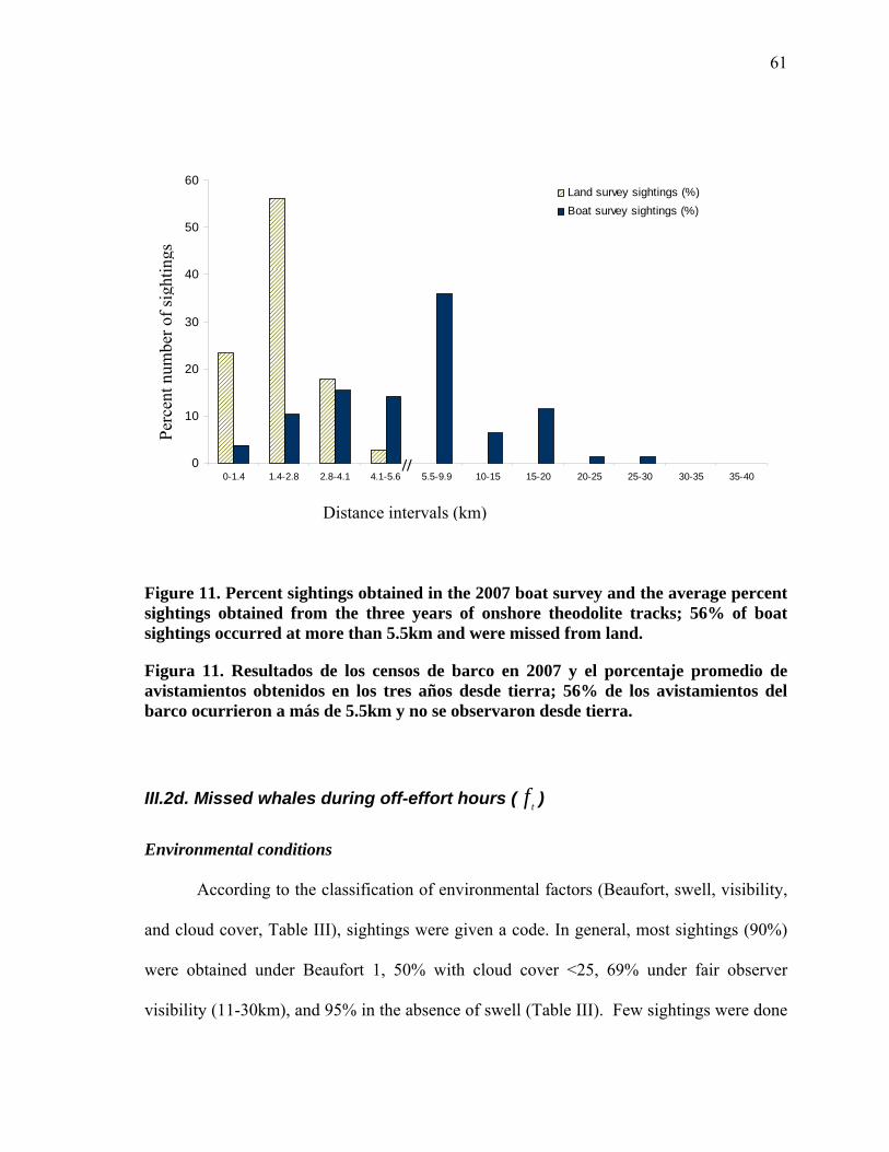
61
igure 11 cent sightings obtained in the 2007 boat survey and the average percent sightings ined from the three years of onshore theodolite tracks; 56% of boat ightings rred at more than 5.5km and were missed from land.
Figura 11. Resultados de los censos de barco en 2007 y el porcentaje promedio de desde tierra; 56% de los avistamientos del
arco ocurrieron a más de 5 n desde tierra.
ere obtained under Beaufort 1, 50% with cloud cover <25, 69% under fair observer
isibility (11-30km), and 95% in the absence of swell (Table III). Few sightings were done
//
F . Perobtaoccus
avistamientos obtenidos en los tres años b .5km y no se observaro
III.2d. Missed whales during off-effort hours ( tf )
Environmental conditions
According to the classification of environmental factors (Beaufort, swell, visibility,
and cloud cover, Table III), sightings were given a code. In general, most sightings (90%)
w
v
0
10
20
0-1.4 1.4-2.8 2.8-4.1 4.1-5.6 5.5-9.9 10-15 15-20 20-25 25-30 30-35 35-40
30
40
50
60Land survey sightings (%)Boat survey sightings (%)
Perc
ent n
umbe
r of s
ight
ings
Distance intervals (km)
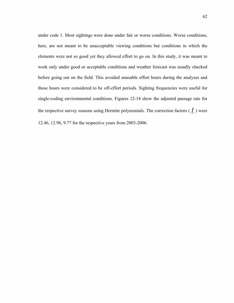
62
under code 1. Most sightings were done under fair or worse co itind ons. Worse conditions,
here, are not meant to be unacceptable viewing conditions but conditions in which the
elements were not so good yet they allowed effort to go on. In this study, it was meant to
work only under good or acceptable conditions and weather forecast was usually checked
before going out on the field. This avoided unusable effort hours during the analyses and
those hours were considered to be off-effort periods. Sighting frequencies were useful for
single-coding environmental conditions. Figures 12-14 show the adjusted passage rate for
the respective survey seasons using Hermite polynomials. The correction factors ( tf ) were
12.46, 12.96, 9.77 for the respective years from 2003-2006.
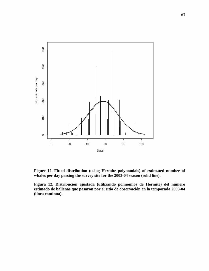
63
020
030
050
040
0
0 20 4 60 80 1000
100
Days
No.
ani
mal
say
per
d
e polynomials) of estimated number of hales per day passing the survey site for the 2003-04 season (solid line).
igura 12. Distribución ajustada (utilizando polinomios de Hermite) del número estimado de ballenas que pasaron por el sitio de observación en la temporada 2003-04
ínea continua).
Figure 12. Fitted distribution (using Hermitw
F
(l
64
0 20 40 60 80 100
020
060
080
010
0040
0
Days
ani
mal
s pe
r day
No.
Figure 13. Fitted distribution (using Hermite polynomials) of estimated number of whales per day passing the survey site for the 2004-05 season (solid line).
Figura 13. Distribución ajustada (utilizando polinomios de Hermite) del número estimado de ballenas que pasaron por el sitio de observación en la temporada 2004-05 (línea continua).

65
200
300
400
100
0
0 20 40 60 80 100
Days
No.
ani
mal
s pe
r day
Figure 14. Fitted distribution (using Hermite polynomials) of estimated number of hales per day passing the survey site for the 2005-06 season (solid line).
igura 14. Distribución ajustada (utilizando polinomios de Hermite) del número estimado de ballenas que pasaron por el sitio de observación en la temporada 2005-06
ínea continua).
w
F
(l
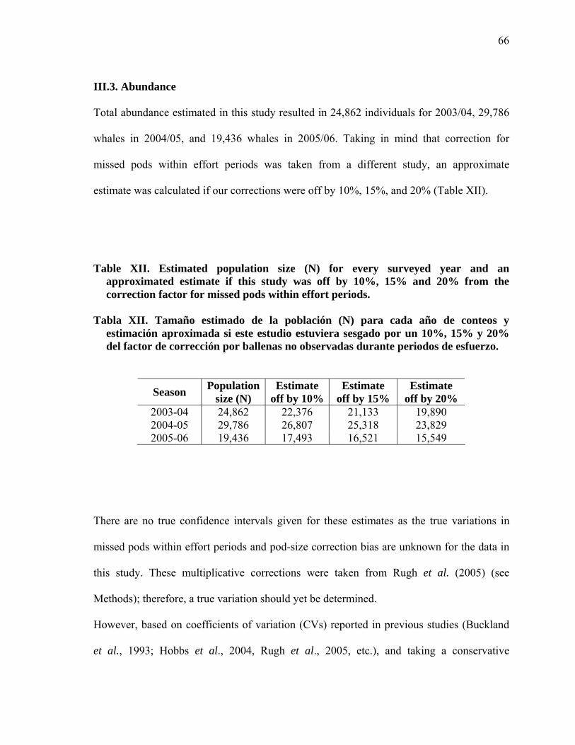
66
III.3. Abundance
Total abundance estimated in this study resulted in 24,862 individuals for 2003/04, 29,786
dy, an approximate
estimate was calculated if our corrections were off by 10%, 15%, and 20% (Table XII).
Table XII. Estimated population siappcorrection factor for missed pods within effort periods.
del factor de corrección por ballenas no observadas durante periodos de esfuerzo.
Season
whales in 2004/05, and 19,436 whales in 2005/06. Taking in mind that correction for
missed pods within effort periods was taken from a different stu
ze (N) for every surveyed year and an roximated estimate if this study was off by 10%, 15% and 20% from the
Tabla XII. Tamaño estimado de la población (N) para cada año de conteos y
estimación aproximada si este estudio estuviera sesgado por un 10%, 15% y 20%
Population size (N)
Estimate off by 10%
Estimate off by 15%
Estimate off by 20%
2003-04 24,862 22,376 21,133 19,890 2004-05 29,786 26,807 25,318 23,829 2005-06 19,436 17,493 16,521 15,549
There are no true confidence intervals given for these estimates as the true variations in
missed pods within effort periods and pod-size correction bias are unknown for the data in
this study. These multiplicative corrections were taken from Rugh et al. (20 ) (see
Methods); therefore, a true variation should yet be determined
05
.
However, based on coefficients of variation (CVs) reported in previous studies (Buckland
et al., 1993; Hobbs et al., 2004, Rugh et al., 2005, etc.), and taking a conservative
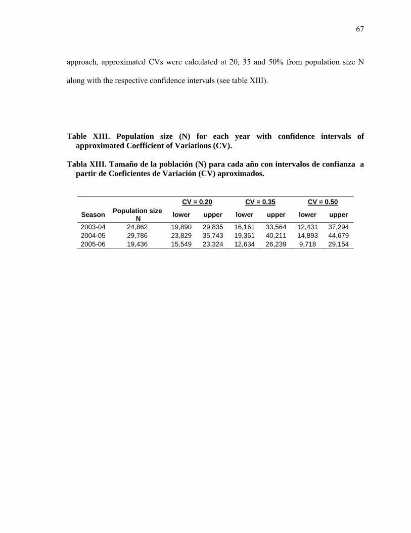
67
approach, approximated CVs were calculated at 20, 35 and 50% from population size N
along with the respective confidence intervals (see table XIII).
Table XIII. Population size (N) for each year with confidence intervals of approximated Coefficient of Variations (CV).
Tabla XIII. Tamaño de la población (N) para cada año con intervalos de confianza a
partir de Coeficientes de Variación (CV) aproximados.
CV = 0.20 CV = 0.35 CV = 0.50
Season Population size N lower upper lower upper lower upper
2003-04 24,862 19,890 29,835 16,161 33,564 12,431 37,294 2004-05 29,786 23,829 35,743 19,361 40,211 14,893 44,679 2005-06 19,436 15,549 23,324 12,634 26,239 9,718 29,154

68
IV. DISCUSSION
IV.1. Migration timing
The timing of the migration for the 2003/04 and 2005/06 survey seasons showed a
consistency. On the other hand, the second survey season (2004-2005) resulted in earlier
migration timing, yet 90% of the sightings, for all three seasons, passed Ensenada at about
the same timing. Delays or early arrivals are not said to be rare, rather they are a reflection
of the population’s behavior to changes in their environment. Rugh et al. (2001) analyzed
data from different sources and estimated an up to 7-day delay in the gray whale’s
southbound migration as well as a delay in the onset of their northbound migration (since
1967). They discuss climate variability and feeding causes, and comment on a “climate
regime shift” occurring in 1970 that may have been linked to the delay. The latter may
explain the low number of individuals estimated by Reilly et al. (1983) in the 1971-72
season. This last statement is not contradicting the conclusion made by Reilly et al. in their
1983 paper, in which they attribute the low estimate to poor visibility conditions. Also,
reported dates cannot de said to be punctual throughout the migration route. Though it was
should have been expected to arrive at a later date in the northbound
igration, yet, no unusual behavior in migration timing was reported for that year.
Data for this study indicate an earlier arrival of the southbound migration in
echanical problems may explain the gaps in the
reported that migration timing was not unusual at Granite Canyon in 1999, LeBoeuf et al.
(2000) find that gray whales were distributed further south in Baja California. According to
this study, whales
m
Ensenada for 2004/05. Bad weather and m
69
obtained data plots about the median dates in the 2004/05 southbound season as well as the
entire migration extension. There was a strong rainy season in January 2005, and the station
provided little protection from the elements. Thus, effort was usually canceled for
consecutive days under bad weather conditions; rainy days in this case. Also, technical
transportation problems limited access to the station for several days and consequently no
effort was undertaken. Nevertheless, more effort hours were dedicated during this season,
in comparison to the previous, and the idea that other external (environmental) factors may
have caused its early arrival cannot be rejected. This can be seen in the migratory relative
abundance index for 2004/05, where the overlap of migration periods is seen during the
mean dates of the southbound migration. Northbound sightings were reported early, just as
the southbound migration had an early arrival. Early or late ice arrival may affect the timing
of grays arriving at certain areas of the migration route. They may be delayed if the ice cap
formation is slow in a given year, having that they may remain more time at the feeding
grounds foraging. On the other hand, one of the factors, aside from daylight (Rugh et al.,
2001), that may trigger an early migration could be a quick ice formation. The covering of
migrating south in the lack of easy food access hence the early arrivals at some sites. Also,
ay only make it as far north as southern Alaska (Rugh et al., 2001). These whales may
ead the southbound migration and hence it may seem that the southbound migration
ming is having an early arrival at the observation site. Apart from the above, distance
ould also take part in peak date determination, since 56% of whales are passing unseen
the feeding grounds by quick ice formation may leave whales no alternative but to start
some whales do not always make it all the way back to the feeding grounds; rather they
m
h
ti
c
offshore.
70
When the southbound distribution of sightings was adjusted with Hermite
les
ere seen. This is true for the southbound migration only, since surveys were still followed
r acquisition of northbound migration data. Rugh et al. (2005) found the southbound
pr dian = 25 January) and they
rep
147km/day, then they should be arriving at Ensenada in approximately 4 days from Granite
Canyon. Wh ared st dian dates at Granite Canyon coincided
with the me obta ring s ars at zul. H this is only
ue for the first and last season, for 2004/05 appeared to be about a week earlier (17-18
January).
polynomials of order 3, the plots did not differ from the adjusted normal bell-shaped curve
(Figs. 12-14). Especially for the 2003/04 plot, the difference is barely noticed. There were
possibly no corrections for missed whales during off-effort periods before the first or after
the last effort day since surveys started early and ended until no more southbound wha
w
fo
migration to be normal in 1997/98 (mean date = 18 January) and 2001/02 (15 January). The
evious year (2000/01) showed a delay in median dates (me
mentioned that it was the most delayed in the past 25 years. In fact, whales were still
orted three weeks after the normal ending date. If whales travel at a speed of
en comp to the late surveys, me
dian dates ined du urvey ye Costa A owever,
tr
71
IV.2. Abundance estimation
VI.2a. Missed whales within effort hours
The calculated corrections for missed whales within effort hours in Granite Canyon
o mination by observers and for missed
tudies been experimented at Costa Azul. Detection probability is assumed to be the same
as that in Granite Canyo are true ded sight arly all
obta hin t ore i a th it n lly.
Unfortunately, the census stations were both at different heights, Costa Azul being the
ighest at 59m above sea level. This height is rather advantageous for allowing a greater
view for it is far higher by more than twice the height than that in Granite Canyon. In 1998,
arsh weather washed out the road to Granite Canyon and a different site was used. Rugh et
l. (2005) made a correction for using a different site (Point Lobos). In 2002, simultaneous
bservations took place in both stations and data were compared based on sightings
ccording to the expected arrival time form one site to the other. A correction for site
ifference between Costa Azul and Granite Canyon was not possible because no
imultaneous observation were undertaken. Despite the facts that in 2007 observations were
nderway at Granite Canyon and also at Costa Azul, the existing data from both sites
annot be comparable. Height difference, weather variability, and offshore distance hinder
nalysis to find a precise correction factor. Hence, the corrections used in Rugh et al.
005) are not fully representative of this area and a true correction factor cannot be derived
have been meticulously studied for years. By using their correction factors, this study
ntemplates a correction for bias in pod size deterc
whales within effort hours as a presumption of what the estimation would be like had those
s
n. At least two factors , the recor ings are ne
ined wit he insh nterval, nd wea er cond ions do ot vary drastica
h
h
a
o
a
d
s
u
c
a
(2
72
for these data. This is why detection probability can only be assumed to be the same when
sing the Granite Canyon corrections for missed whales during effort periods and bias
ction probability is higher at Costa Azul then abundance is
being underestimated. Assuming that this study is overestimating the counted whales and
our correction (had this study calculated these corrections) would be off by 10%, the final
estimate would then be 22,376 for 2003/04, 26,807 for 2004/05 and 17,493 for 2005/06.
Estimates would be even lower if this study was off by 20% totaling 19,890, 23,829, and
15,549 for the respective years from 2003-2006 (Table XII). If, in fact, detection
probability of a pod is about the same at Costa Azul, then under- or overestimation of the
population may be explained with the 56% percent passing offshore.
d er from
shore than what was initially expected.
u
correction in pod size. If dete
VI.2b Pods missed due to distance from shore
The migration corridor can vary between years and at the same time distance
offshore can vary between sites. At Granite Canyon, studies have recorded that observers
there are seeing most of the passing whales, and in fact most of the population passes
within the inshore distance interval (5.6km) (Shelden and Laake, 2002). On the contrary,
there are sites in which whales expand their migration corridor such as Washington and
Oregon (Green et al., 1995), where whales were observed 40km from the coast. Observers
at Costa Azul are missing a great percentage of whales due to distance, needing a correction
factor for missed whales ( f =1.56). Surprisingly, most grays are passing furth
73
Ensenada forms a bay, and perhaps, as an energy-saving mechanism, whales may be
taking a straight migration route rather than wasting energy by shoring the bay. In their
study, Green et al. (1995) suggest that a portion of the gray whale population takes a more
direct offshore route in Washington, U.S.A. Green et al. (1995) also hypothesize the
possibility of whales migrating according to depth, i.e. they tend to follow shallow 100-150
m deep waters rather than crossing the deep Juan de Fuca submarine canyon (250-650 m).
That is, it may seem that gray whales are crossing the Juan de Fuca submarine canyon, in
the southern Gulf of Alaska, “at its narrowest point” by following an offshore route towards
Washington and maintain that offshore route, since the shallow waters here “extend 75km
from shore” (Green et al., 1995).
Cartography in northern Mexico shows shallow waters extending ≈18km from the
Rosarito (a town ≈50km north of Costa Azul) coast (Legg, 1985). A steep slope drops off
5km from the Ensenada coast to a depth of 250m (Fig. 15). Shallow waters (≈ 100 m) are
again seen <5km from Punta Banda and further south the underwater Soledad Ridge
(≈40km south from the observation point) allows a ≈ 100 m deep shallow region ≈18km
from the continental coast. These shallow depths follow south to the wide Santo Tomás
shelf (located ≈50km from Costa Azul and ≈10km from Punta Banda). If whales are routing
by topography, then they may be following a direct path from Rosarito town to the shallow
waters in any of the Punta Banda coast, Soledad ridge or Santo Tomás shelf points (Fig.
15). Further, the Todos Santos islands found west of Todos Santos bay are almost aligned
with the Punta Banda peninsula. This may form a small barrier

74
Figure 15.- Bathymetry map south of the observation site showing Santo Tomás shelf and Soledad Ridge. This study’s observation point is located near punta Salsipuedes (Legg, 1985).
igura 15.- Mapa batimétrico del sur del sitio de observación mostrando la omás y la cresta de la Soledad. El punto de observación de este
studio se localiza cerca de punta Salsipuedes (Legg, 1985).
Fplataforma de Santo Te

75
for whales to migrate closer to the shore as it may seem as a coastal route for grays and
therefore a direct southward route may be taken. If so, this may, perhaps, be a mean of
saving energy cost by evading entrance to the Ensenada bay. In fact, the mother and calf
apair th t was observed at about 40km from the coast heading south can possibly evident
this thought. A more profound study is recommended to test this hypothesis.
Onshore and boat surveys were both used to find the percent of whales missed due
to a limited distance view. If all gray whale sightings with a position from the theodolite
had been analyzed then perhaps, a greater percentage could have been recorded further off
the coast. According to boat survey results, whales were still reported from 30 to 35km,
though they were not included in the analysis because they did not fall within the strip
width. Boat survey sample size would have been greater if all sightings had fallen within
the strip width, nonetheless and even if more than half the recorded sightings were not
included, sample size was sufficient. When exploring all sightings, the distribution was not
much different from the valid sample size results.
Other studies (Shelden and Laake 2002) have found that the migration corridor may
vary between years yet this cannot be confirmed at Costa Azul only from shore
observations, in view of the wide migratory corridor at this site as boat survey results
showed. The correction factor for distance from shore elevated the total number of whales
estimated for this population. Abundance estimates may be overestimated if distance is
underestimated and the reverse is also true (Kinzey and Gerrodette, 2003). Variations in
this correction may be present because no paired boat surveys were done to account for
observer discrepancies here. Kinzey and Gerrodette (2003) analyzed the precision of
measuring distance at sea using reticles in binoculars. A possible bias may occur in
76
determining the reticle line, especially under swell conditions. The above mentioned
authors found that underestimation occurs from using reticle measurements and although
refraction may affect, swell height, Beaufort Sea state and wind speed caused greater
affects on reticle measurements. Paired boat surveys were not possible due to a budget
limitation, nevertheless having that an important number of whales is being missed this
correction factor should be considered valid, until new research is done in this zone. During
the boat surveys, at Ensenada, bad weather prevailed and it is most probable that the
resulting reticle measurements are biased due to swell height and Beaufort Sea state. If
distance obtained from reticle measurements is underestimated, then this in part explains
the high abundance estimates for all three years.
Percent sighting distribution within inshore distances in Ensenada turned out the
same as that in Shelden and Laake (2002), which is the distance where most observations
are reported. Observers are seeing most of the recorded sightings within inshore (5.5km).
As a result, from theodolite tracks, the observer is seeing only up to 5.5km, this defines the
eye sight limitation from shore to sea. This gives away the distance of the field viewing
range at the observation site. Observer eye sight limitation can be taken as such distance,
since comparisons with boat survey results indicate that there are significant numbers of
whales still passing beyond this distance. Although the theodolite’s telescope (30X) does
aid to identify at a greater distance than regular 7X50 binoculars, observers still have a
limited view range. The migration corridor in Ensenada can be said to be quite ample, from
y at certain sites of their migration route or so is
1km off the coast extending to perhaps more than 30km out sea, at least for 2007. Gray
whales show to be coastal migrants onl
77
seen in
VI.2c. Missed whales during off-effort periods
fort was not done all 7 days a week or if visibility is a
“seriou
compared results (Figure 9) from aerial surveys at Granite Canyon and reports in
Green et al. (1995).
The use of Hermite polynomials became rather advantageous allowing interpolation
within a density curve, accounting for periods on which no counts took place. Unlike
Hermite polynomials, other methods, such as Kernal estimation, will not allow any
computations unless there are no gaps in our data (there are no missing effort periods).
Polynomial adjustment is used if the parametric fit is not adequate. Estimation remains
reliable even if, as in this case, ef
s handicap” (Buckland, 1992). Of all correction factors estimated in this study, this
is the most confident. Visibility periods were meticulously categorized for the output data
used in the gwnormf77 FORTRAN R statistical program. Though a confident estimated
correction factor, the elevated number of individuals could have come from these
estimations. Nonetheless, the source error could have also derived from the database in the
first place. There are high numbers of individuals in such small time intervals, when
compared to the other two years. These high numbers are indicated on the plots for 2004/05
data (Fig. 13). Since Hermite fitting adjusts the curve and hence interpolation is possible
then, perhaps, the high peaks are sourcing the error. Abundance estimates were quite high
in 2004/05 and very low in 2005/06. Biases may have altered the numbers, though a pattern
of ascent and descent is evident.

78
VI.2d. Abundance
Gray whale abundance in Ensenada during three migration seasons (2003-2006),
had an apparent increase in 2004-05 (29,786), with respect to the preceding year (24,862,
and a drop of a bit over 10,000 individuals in the subsequent year (19,436). The high
numbers may be attributed to bias in analyses due to lack of experiments to correctly or
precisely account for factors that determine final estimates. Nevertheless, this indicates that
there might have been an increase of animals from the last estimates reported in 2002.
Springer (2000), discuss that there has been a 30% decrease in the Chuckchi-Beaufort
ecosystem and other authors claim the Eastern Pacific stock of gray might be reaching an
equilibrium level (Hobbs et al., 2004; Wade, 2002). Considering this, the drop in number of
individuals in the 2005/06 season may have been due to the natural behavior of a
population after reaching k. If food availability has dropped in the past years and the
number of whales has increased considerably, then this is the major limiting factor
controlling the population. The ecosystem can bear only a certain amount of whales. Le
Boeuf et al. (2002) state that the high mortality rates reported in 1999 may have been due to
a “decrease in their principle prey.” In fact, Rugh et al. (2001) report that some whales have
been sought feeding further north of the Beaufort Sea, near Canada, meaning that whales
ehavior of gray whale population size in the past years (1996-2006) is
iewed in a graphic manner (e.g. Fig. 16), this fluctuation would be pictured as the number
opulation would be found in a stable balance point, according the Allee effect
are traveling further north in the seek of food.
If the b
v
of individuals in a population moving above and below the carrying capacity level. The
p
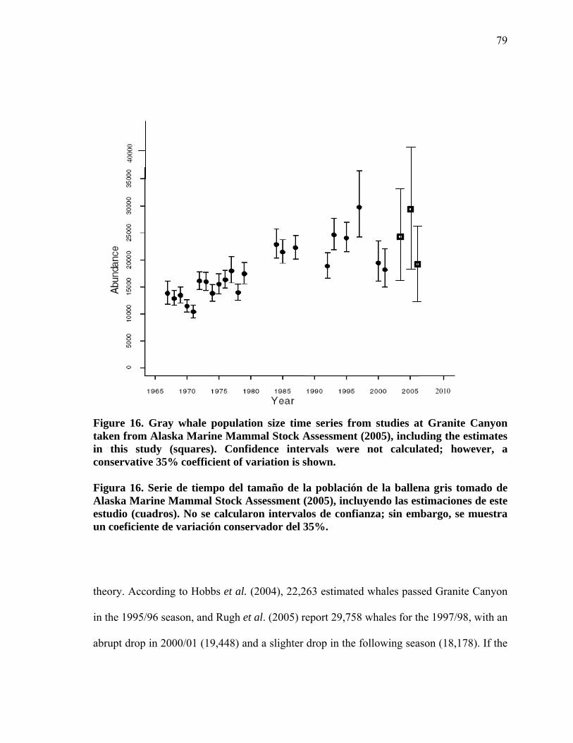
79
ies from studies at Granite Canyon taken from Alaska Marine Mammal Stock Assessment (2005), including the estimates in thisconservative 35% coefficient of variation is shown.
Figura 16. Serie de tiempo del tamaño de la población de la ballena gris tomado de
estudio (cuadros). No se calcularon intervalos de confianza; sin embargo, se muestra
theory. According to Hobbs et al. (2004), 22,263 estimated whales passed Granite Canyon
in the 1995/96 season, and Rugh et al. (2005) report 29,758 whales for the 1997/98, with an
abrupt drop in 2000/01 (19,448) and a slighter drop in the following season (18,178). If the
Figure 16. Gray whale population size time ser
study (squares). Confidence intervals were not calculated; however, a
Alaska Marine Mammal Stock Assessment (2005), incluyendo las estimaciones de este
un coeficiente de variación conservador del 35%.
2010
4000
0

80
pattern is followed with the results from this study, then an increase in number of
individuals is observed in 2003/04 reaching a peak in the subsequent year (29,786) and a
decrease is followed in 2005/06 (Fig. 16).
Coefficients of variation (CVs) were not calculated in this study because average
corrections for missed pods during effort hours (detection probability) and pod size
observer bias were taken from studies at Granite Canyon (Rugh et al., 2005). A true CV
calculation should be made taking this factor into account. Approximated CV values gave
an idea of this study’s CV range. Coefficients of variation greater than 35% gave off very
low values in the lower confidence intervals (e.g. 12,634 whales in 2005-06). Also, past
abundance estimates (Reilly et al., 1983; Buckland et al., 1993, Hobbs et al., 2004 and
Rugh e
t al., 2005), have not reported confidence intervals below 13,000 or beyond 40,000
individuals (CVs ranged from 0.20 to 0.35). Given the confidence intervals in table XIII
and from past reports at Granite Canyon, our estimates might range in a 20 to 35% CV. The
final estimated population size (N) of every season is higher than the latest reports from
Granite Canyon (2000-01: 19,448 whales; 2001-02: 18,178 whales; Rugh et al., 2005)
though the N reported in the last season (19,436) is not far off from the last estimated year
there (2001/02). The estimation of that year was 18,178 whales with 95% confidence
intervals ranging from 15,010 to 22,015 (Rugh et al., 2005).
81
V. CONCLUSIONS Migration timing
few days in the three years of this
tudy, though for 2004/05 this variation was more noticeable with an early start of
Gray whale abundance consisted in separate analyses; correction factors (day/night
travel rate, pod size and missed pods within effort periods, missed pods because of
distance, and missed pods during off-effort periods) were used in the final estimated
from results of past experiments at Granite Canyon because no such research was
done during the three mentioned years. For missed pods because of distance
offshore, an experiment was done in 2007 about the dates of the peak of the
migration. This experiment included boat surveys near the onshore survey station
• Timing for the southbound migration varied a
s
nearly a week (December 25 vs. January 2 and 6).
• The early arrivals in migration timing could be explained by quick ice formation at
the feeding grounds, forcing whales to leave before the usual timing. Also, whales
residing south of Alaska may head the southbound migration, and so early dates.
• Northbound gray whales without calves, migrating back to the feeding grounds, past
Ensenada around similar dates (18-19 April).
• While in the first and last surveyed years mothers and calves had ended their
migration past the station in late April, in 2004/05 migration ended in 05 May. This
showed an ample migration distribution for this year.
Abundance estimation
•
population size. The corrections for whales missed within effort periods were taken
82
and gray whale theodolite tracks. Missed pods during off-effort periods were
accounted for by fitting the sighting’s distribution with Hermite polynomials.
• Though most correction factors were taken into account, other correction factors,
such as observer fatigue, should still be taken into account in further research.
• Some possible biases in the final estimation may have derived from using the
detection probability obtained at Granite Canyon and observer fatigue.
Nevertheless, a great percentage of missed whales was corrected for with the results
from boat surveys. Observers are missing 56% of the population because they are
passing too far offshore. It may be assumed that topography is playing a role in the
offshore distribution as in other sites (e.g. Washington, U.S.A.).
• Hermite polynomial fitting also provided an increase in the final estimation, since
surveys did not take place everyday of the week and off-effort periods were
frequent. Although bias may have come mainly from missed whales during effort
periods, the analyses indicate a small pattern.
• Gray whale abundance in Ensenada was estimated to be 24,862, 29,786, and 19,436
during the years 2003-2004, 2004-2005, and 2005-2006.
• Coefficients of variation were approximated for the final population size, as a lack
of experiment and data did not allow a true CV estimation. However it should be
noted that our CV may range from 20 to 35%. In all, the population fluctuated in
these three years and it seemed to have decreased in the last surveyed year.
Comparisons should still be done with the estimation obtained at Granite Canyon
for 2006/07 to see how biased these estimations are.
83
VI. LITERATURE CITED
ngton. ess, Seattle, 107 p.
Baird, R.W., Stacy, P.J., Duffus, D.A. and Langellier, K.M. 2002. An evaluation of gray
whale (Eschrichtius robustus) mortality incidental to fishing operations in British Columbia, Canada. Journal of Cetacean Research and Management. 4(3): 289-296 p.
Blokhin, S.A., Maminov, M.K. and Kosygin, G.M. 1985. On the Korean-Okhotsk
population of gray whales. Report of the International Whaling Commission, 35. SC/36/PS7.
Bowen, S.L. 1974. Probable extinction of the Korean stock of gray whale (Es richtius
robustus). Journal of Mammalogy. 55(1): 208-209 p. Brownell, R.L. and Chun, C. 1977. Probable existence of he Korean stock of gray whale
(Eschrichtius robustus). Journal of Mammalogy. 58(2): 237-239 p. Bryant, P.J. 1995. Dating remains of gray whales from the eastern North Atlantic. Journal
of Mammalogy. 76(3): 857-961 p.
arine Mammal Science. 9(3): 235-
ew York. 431p.
etacean Specialist Group. 1996. Eschrichtius robustus. In: IUCN 2006. 2006 IUCN Red List of Threatened Species. www.iucnredlist.org
Allen, K.R. 1980. Conservation and Management of Whales. University of WashiPr
ch
Buckland, S.T. 1992. Fitting density functions with polynomials. Applied statistics, 41, 63-76 p.
Buckland, S.T., Breiwick, J.M., Cattanach, K.L. and Laake, J.L. 1993. Estimated
population size of the California gray whale. M249 p.
Buckland, S.T., Anderson, D.R., Burnham, K.P., Laake, J.L., Borchers, D.L., and Thomas,
L. 2001. Introduction to Distance Sampling. Estimating abundance of biological opulations. Oxford University Press. 1a ed. Np
C. [Accessed 18 August 2007].
Cipriano, F. 1990. User’s Manual T-TRAK Version 1.0. Theodolite-Tracking Data Analysis (for IBM-compatible computers). University of Arizona (unpublished). 38 p.
Clapham, P.J., Young, S.B. and Brownell, R.L. 1999. Baleen whales: conservation issues
and the status of the most endangered populations. Mammal Review 29: 35-60 p.
84
(Eastern North Pacific population) Eschrichtius robustus in Canada. Committee on COSEWIC. 2004. COSEWIC assessment and update status report on the grey whale
the Status of Endangered Wildlife in Canada. Ottawa, Canada. vii + 31 p. _e.cfmwww.sararegistry.gc.ca/status/status . [Accessed July 2007].
CSDS
almacenamiento y regasificación de gas natural licuado. Available from
(Continental Shelf Data Systems). 1971. Todos Santos South. Bathymetric Map. Denver, Colorado, USA.
Energía Costa Azul. 2007. Manifestación de Impacto Ambiental. Terminal de recibo,
http://www.energiacostaazul.com.mx/files/CAP7.pdf [Accessed 15 August 2007].
Findley, L. T. and O. Vidal (2002). "Gray whale (Eschrichtius robustus) at calving sites in
the Gulf of California, México." Journal of Cetacean Research and Management 4(1): 27-40 p.
Gard, R. 1974. Aerial Census of gray whales in Baja California lagoons, 1970 and 1973,
with notes on behavior, mortality and conservation. California Fish and Game. 60(3): 132-143 p.
Gilmore, R.M. 1960. A census of the California gray whale. US Fish and Wildlife Service
Special Scientific Report. Fisheries, 342, 1–30 p. Gilmore, R.M., Brownell, R.L., Jr., Mills, J.G., and Harrison, A. 1967. Gray whales near
Yavaros, Southern Sonora, Golfo de California, Mexico. San Diego Society of Natural History. 14(16): 197-204 p.
Green, G.A. Brueggeman, J.J., Grotefendt, R.A.,a nd Bowly, E. 1995.Offshore distance of
gray whales migrating along the Oregon and Washington coasts, 1990. Northwest Science. 69(3); 223-227 p.
Gulland, F.M.D., H. Perez Cortes M., J. Urban R., L. Rojas-Bracho, Ylitalo, G. Weir, J.,
Norman, S.A., Muto, M.M., Rugh, D.J., Kreuder, C.,
and Rowels, T. 2005. Eastern Eschrichtius robustus) unusual mortality event, 1999-
000. U.S. Dep. Commer., NOAA Tech. Memo. NMFS-AFSC-150, 33p. Heckel, Gisela. 2001. Influencia del ecoturismo en el comportamiento de la ballena gris
Todos Santos, Baja California, y aguas dyacentes: Propuesta de un plan de manejo. Tesis de Doctorado, Facultad de
Ciencias Marinas, UABC. México. 109 p.
North Pacific gray whale (2
(Eschrichtius robustus) en la Bahía de a
85
Henderson, D.A. 1984. Ninpractices and depletio
eteenth century gray whaling: grounds, catches and kills, n of the whale population. Pp. 159-200. In: Jones, M.L.,
. and S. Leatherwood (eds.) The gray whale, Eschrichtius robustus. ress, Inc. Orlando, Florida. xxiv+600 p.
Hic y
Highsmith, R.C. and Coyle, K.O. 1992. Productivity of arctic amphipods relative to gray
Hobbs,
eastern North Pacific gray whales on the 1995/96 southbound migration. Journal of
Hu
Fish and Game. 53(1): 23-27 p. International W e Scientific Committee. Report of
International W
g. Annex 5. USA: Statement 9: 16 p.
ission. 2007c. Report of the Scientific Committee.
International W
Jones,
Kinzey
Swartz, S.LAcademic P
ke , B.M. 1993. Physical oceanography. In: M.D. Dailey, D.J. Reish y J.W. Anderson
(eds), Ecology of the Southern California Bight. A Synthesis and Interpretation. Univ. California Press, Berkeley, 19-70 p.
whale energy requirements. Marine Ecology Progress Series. (83): 141-150 p.
R.C., Rugh, D.J., Waitte, Breiwick J.M. and DeMaster D.P. 2004. Abundance of
Cetacean Research and Management. 6(2): 115-120 p.
bbs C.L. and Hubbs, L.C. 1967. Gray whale census by airplane in Mexico. California
haling Commission. 2007a. Report of ththe Sub-Committee on Aboriginal Subsistence Whaling. J. Cetacean Res. Manage. (Suppl.) 9: 3-6 p.
haling Commission. 2007b. Report of the Scientific Committee. Report of the Sub-Committee on Aboriginal Subsistence Whalinon the Makah needs statement. J. Cetacean Res. Manage. (Suppl.)
International Whaling Comm
SC/59/BRG40. Brownell, R.L., Jr., Makeyev, C.A.F. and Rowles, T.K. Stranding trends for eastern gray whales, Eschrichtius robustus: 1975-2006.11 p.
haling Commission. 2007 d. Report of the Scientific Committee. SC/59/BRG1. Rugh, D., Muto, M., Hobbs, R., Shelden, K., D’Vincent, C., Laursen, I.M. , Reif, S., Maher, S. and Nilson, S. Field report of the 2006/07 Census of the Eastern North Pacific stock of gray whales. 9 p.
M.L. and Swartz, S.L. 2002. Gray whale (Eschrichtius robustus). In: Perrin, W.F., Würsig, B.,and Twewissen, J.G.M. Encyclopeda of marine mammals. Academic Press. San Diego. 524-536p.
, D. and Gerrodette, T. 2001. Conversion factors for binocular reticles. Mar. Mammal Sci. 17(2): 353-61 p.

86
Kinzeysea: accuracy, precision and effects of refraction. Journal of Cetacean Management.
Lill o
Skand. Naturf., 8 de Møde, Kjöbehavn, 1860:599-616 p. Le Boeuf B.J., H.Pérez-Cortés M., Urbán R.J., Mate, B.R. and Ollervides U.F. 2000. High
implications. Journal of Cetacean Research Management, 2(2): 85-99 p. Legg, M. 1985. Inner California continental borderland. Bathymetric chart. U.S.A. Mapa de Mexico.2007. http://www.hablandodesigs.com/openlayers/mapademexico.html
, D. and Gerrodette. 2003. Distance measurements using binoculars from ships at
5(2):159-171 p.
jeb rg, W. 1861. Hvalben funna I jorden på Gräsön Roslagen i Sverige. Forhandl.
gray whale mortality and low recruitment in 1999: potential causes and
.
Mate, B
Hatfield Marine Science Center, Newport Oregon. MBC Applied Environmental Sciences. 1989. Gray whale monitoring study; final report.
Mizue,
Institute, Tokyo. 5:71-79 p. NOAA fisheries, Office of Protected Resources. 2002. Gray Whale Stock Assessment.
gov/prot_res/PR2/stock_Assessment_
[Accessed July, 2007].
. 1999. Marine Mammal program report, August 1999. Oregon State University,
Costa Mesa, California. 95 p.
K. 1951. Gray whales in the East Sea area of Korea. Sci. Rep. Whales Research
Available from http://www.nmfs.noaa.Program/Cetaceans/Gray_Whale_(Eastern_N._Pacific)/AKO2graywhale_E.N.Pacific.pdf. [Accessed July 2005].
J.S. and Slattery, P.N. 1985. Destruction and opportunity ogray whale feeding. Ecology. 66(6): 1965-1975 p.
Oliver, n the sea floor: effects of
Perrym
Perrym
Pike, G
an, W.L. Donahue, M.A., Laake, J.L. ad Martin, T.E. 1999. Diel variation in migration rates of eastern Pacific gray whales measured with therma imaging sensors. Marine Mammal, Science. 15 (2): 426-425 p. an, W.L., Donahue, M.A., Perkins, P.C. and Reilly, S.B. 2002. Gray whale calf production 1994-2000: Are observed fluctuations related to changes in seasonal ice cover? Marine Mammal Science 18: 121-144 p.
.C. 1962. Migration and feeding of the gray whale (Eschrichtius gibbosus). J. Fish. Res. Bd. Can. 19(5): 815-38 p.

87
Reeves, R.R., B.S. Stewart, P.J. Clapham and J.A. Powell. 2002. National Audubon Society e World. Chanticleer Press, Inc. Nueva York, Nueva
n 30: 359-368 p.
Science. 6 (2):
ugh, M.E., Boucher, G.C. 1993. A comparison of
ugh, 2002. evaluation of
rnal of Cetacean Research Management. 7 (1): 1-12 p.
Guide to Marine Mammals of thYork, EE.UU. 527 p.
Reilly, S.B., Rice, D.W. and Wolman, A.A. 1980. Preliminary population estimate for the
California gray whale based upon Monterrey shore censuses, 1967/68 to 1978/1979. Rep. Int. Whal. Comm
Reilly, S.B., Rice, D.W. and Wolman, A.A. 1983. Population Assessment of gray whale,
Eschrichtius robustus, from California shore censuses, 1967-1980. Fishery Bulletin: Vol. 81 (2): 267-281 p.
Reilly, S.B. 1984. Assessing gray whale abundance: A review. Pp. 203-223. In: Jones,
M.L., Swartz, S.L. and S. Leatherwood (eds.) The gray whale, Eschrichtius robustus. Academic Press, Inc. Orlando, Florida. xxiv+600 p.
Rice, D.W. and A.A. Wolman. 1971. The life history and ecology of the gray whale
(Eschrichtius robustus). The American Society of Mammalogists, Special Publication #3, 131 p.
Rugh, D.J., Ferrero, R.C., Dahlheim, M.E. 1990. Inter-count discrepancies in a shore-based
census of gray whales (Eschrichtius robustus). Marine Mammal109-120 p.
D.J., Breweick, J.M., Dahlheim, Rindependent, concurrent sighting records from a shore-based count of gray whales. Wildlife Society Bulletin. 21: 427-437 p.
Rugh, D.J. Muto, M.M., Moore, S.E., and DeMaster, D.P. 1999. Status review of the
Eastern North Pacific stock of gray whales. U.S. Dep. Of Commer., NOAA Technical Memorandum NMFS-AFSC-103. 93 p.
Rugh, D.J., Shelden, K.E.W. and Schulman-Janiger, A. 2001. Timing of the gray whale
southbound migration. Journal of Cetacean Research Management: 3 (1): 31-39 p.
D.J., Lerckzak, J.A., Hobbs, R.C., Waite, J.M., and Laake,J.L. Rhigh-powered binoculars to detect inter-year changes in offshore distribution of eastern North Pacific gray whales. Journal of Cetacean Research Management. 4 (1): 57-61 p.
Rugh, D.J., R.C. Hobbs, J.A. Lerckzak, and J.M. Breiwick. 2005. Estimates of abundance of eastern North Pacific stock of gray whales (Eschrichtius robustus) 1997-2002. Jou
Spatz, C. and Johston, J.O. 1989. Basic Statistics. Tales of distribution. 4th ed. Brooks/Cole
Publishing company. Pacific Grove, California.U.S.A.
88
Scammon, C.M. (ed.). 1874. The Marine Mammals of the North-western Coasts of North
America, Described and Illustrated: Together with an Account of the American Whale-fishery. John H. Carmany and Co., San Francisco. x+319+vpp. [reprinted in 1968 by Dover Publications, Inc., New York].
SEMARNAT (Secretaría de Medio Ambiente y Recursos Naturales). 2002. Norma Oficial
Mexicana NOM-059-ECOL-2001, Protección ambiental-Especies nativas de México de Flora y Fauna Silvestres-Categorías de riesgo y especificaciones para su inclusión, exclusión o cambio-Lista de especies en riesgo. Diario Oficial de la
Shelde f
southbound migrating gray whales from aerial survey data collected off Granite
Springer, A. 2000. Climate change and mImpacts of Changes in Sea Ice and Other Environmental
haling Comm. 37:295-299
Towns
Federación, 6 de marzo de 2002.
n, K.E.W. and Laake, J.L. 2002. Comaprison of the offshore distribution o
Canyon, California, 1979-1996. Journal of Cetacean Management. 4 (1): 53-6 p.
arine ecosystems of the western Arctic. In: H.P. Huntington (ed.) Parameters in the Arctic. Final Report of the Marine Mammal Commission Workshop, Girdwood, Alaska, 15-17 February 2000. Marine Mammal Commission, Bethesda,Maryland.
Swartz, S.L., Jones, M., Goodyear, J., Withrow, D. E., and, Miller, R.V. 1987. Radio-
telemetric studies of gray whale migration along the California coast: a preliminary comparison of day and night migration rates. Rep. Int. Wp.
end, C.H. 1887. Present condition of the gray whale fishery. Bull. U.S. Fish. Comm. 6, 340-350 p.
Wade, P.R. 2002. A Bayesian stock assessment of the eastern Pacific gray whale using
abundance and harvest data from 19678-1996. Journal of Cetacean Research Management. 4(1):85-98 p.

89
ANNEX I
ons used in the calculation of whales passing the survey within effort hours Equati
Total n e
3
umber of pods of size e passing during the effort periods, M :
∑=∧ em
M1
E=i eipe 1
q. (5)
and its variance is obtained through:
⎟⎞⎜⎛∑⎟⎞⎜⎛+⎥⎠⎝⎠⎝⎥⎦⎢
⎤⎢⎣
⎡ −=⎟⎞⎜⎛
∧
∑T
em
MVarp1
⎠⎝ =iei
p1
detection probabili
∧∧∧
eeei
e MDMD βββ2 Eq. (6)
ei= ty of the ith pod of size e.
em = n
p
umber of pods of size e sighted from the primary site.
β = vector of parameters
⎞∧
ˆ⎟⎜⎛M = vector of partial derivatives of M with respect to ⎠⎝ eβ eD β .
β
∧
∑ = estimated variance-covariance matrix of the vector of parameter estimates ( β ).
(c.f. Borchers et al, 1996).
3 All equations and description of variables are after Hobbs et al., 2004.
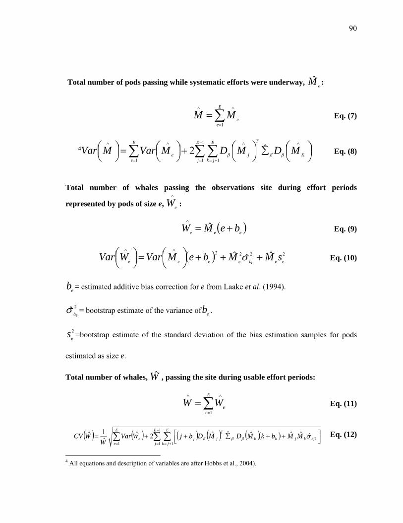
90
Total number of pods passing while systematic efforts were underway, eM :
∑=
= MM Eq. (7)
4 ⎟⎜∑⎟+⎟⎜=⎟⎜ ∑∑∑ MDMDMVarMVar 2 Eq. (8)
Total assing the observations site during effort periods ∧
ˆ
2222⎞⎛⎞⎛
∧∧ E
ee
1
⎞⎛⎞⎛⎞⎛⎞⎛ ∧− ∧∧∧ E E TE 1
ˆ⎠⎝⎠⎝⎠⎝⎠⎝ = +==
Kj jk
jee
βββ1 11
⎜
number of whales p
represented by pods of size e, eW :
∧
( )eee beMW += Eq. (9)
∧∧
( ) ˆˆˆeeebeeee sMMbeMVarWVar +++⎟
⎠⎜⎝
=⎟⎠
⎜⎝
σ Eq. (10)
eb = estimated additive bias correction for e from Laake et al. (1994).
2ˆ ebσ = b e
l n
ootstrap estimate of the variance ofb .
2es =bootstrap estimate of the standard deviation of the bias estimation samples for pods
estimated as size e.
umber of whales, W , passing the site during usable effort periods: Tota
∑=
(
∧∧
=E
eeWW
1
Eq. (11)
) ( ) ( ) ( ) ( )( )∑ ∑∑−
⎢⎣⎡ ++=
1
2ˆˆ1ˆ
E E TE
e bjWVar= +==
⎥⎦⎤++∑
1 11
ˆˆˆˆˆˆj jk
bjkkjkkjje
MMbkMDMDW
WCV σβββ Eq. (12)
4 All equations and description of variables are after Hobbs et al., 2004).