gravitational waves - zarm: zarm · pdf filegravitational waves claus l¨ammerzahl...
TRANSCRIPT

Gravitational Waves
Claus Lammerzahl ([email protected])
Volker Perlick ([email protected])
Summer Term 2014
Tue 16:00–17:30 ZARM, Room 1730 (Lectures)
Fr 14:15–15:00 ZARM, Room 1730 (Lectures)
Fri 15:00–15:45 ZARM, Room 1730 (Tutorials)
Complementary Reading
The following standard text-books contain useful chapters on gravitational waves:
S. Weinberg: “Gravitation and Cosmology” Wiley (1972)
C. Misner, K. Thorne, J. Wheeler: “Gravitation” Freeman (1973)
H. Stephani: “Relativity” Cambridge University Press (2004)
L. Ryder: “Introduction to General Relativity” Cambridge University Press (2009)
N. Straumann: “General Relativity” Springer (2012)
For regularly updated online reviews see the Living Reviews on Relativity, in particular
B. Sathyaprakash, B. Schutz: “Physics, astrophysics and cosmology with grav-itational waves” htp://www.livingreviews.org/lrr-2009-2
Contents:
1. Historic introduction
2. Brief review of general relativity
3. Linearised field equation around flat spacetime
4. Gravitational waves in the linearised theory around flat spacetime
5. Generation of gravitational waves
6. Gravitational wave detectors
7. Gravitational waves in the linearised theory around curved spacetime
8. Exact wave solutions of Einstein’s field equation
9. Primordial gravitational waves
1

1. Historic introduction
1915 A. Einstein establishes the field equation of general relativity
1916 A. Einstein demonstrates that the linearised vacuum field equation admits wavelike so-lutions which are rather similar to electromagnetic waves
1918 A. Einstein derives the quadrupole formula according to which gravitational waves areproduced by a time-dependent mass quadrupole moment
1925 H. Brinkmann finds a class of exact wavelike solutions to the vacuum field equation, latercalled pp-waves (“plane-fronted waves with parallel rays”) by J. Ehlers and W. Kundt
1936 A. Einstein submits, together with N. Rosen, a manuscript to Physical Review in whichthey claim that gravitational waves do not exist
1937 After receiving a critical referee report, A. Einstein withdraws the manuscript with theerroneous claim and publishes, together with N. Rosen, a strongly revised manuscript onwavelike solutions (Einstein-Rosen waves) in the Journal of the Franklin Institute
1957 F. Pirani gives an invariant (i.e., coordinate-independent) characterisation of gravitationalradiation
1960 I. Robinson and A. Trautman discover a class of exact solutions to Einstein’s vacuumfield equation that describe outgoing gravitational radiation
1960 J. Weber starts his (unsuccessful) search for gravitational waves with the help of resonantbar detectors (“Weber cylinders”)
1974 R. Hulse and J. Taylor (Nobel prize 1993) discover the binary pulsar PSR B1913+16 andinterpret the energy loss of the system as an indirect proof of the existence of gravitationalwaves
2002 The first laser interferometric gravitational wave detectors go into operation (GEO66,LIGO, VIRGO,...)
2014 BICEP2 finds evidence for the existence of primordial gravitational waves in the cosmicbackground radiation
2
2. Brief review of general relativity
A general-relativistic spacetime is a pair (M, g) where:
M is a four-dimensional manifold; local coordinates will be denoted (x0, x1, x2, x3) and Ein-stein’s summation convention will be used for greek indices µ, ν, σ, . . . = 0, 1, 2, 3 and for latinindices i, j, k, . . . = 1, 2, 3.
g is a Lorentzian metric on M , i.e. g is a covariant second-rank tensor field, g = gµνdxµ ⊗ dxν ,
that is
(a) symmetric, gµν = gνµ, and
(b) non-degenerate with Lorentzian signature, i.e., for any p ∈ M there are coordinatesdefined near p such that g|p = −(dx0)2 + (dx1)2 + (dx2)2 + (dx3)2.
We can, thus, introduce contravariant metric components by
gµνgνσ = δµσ.
We use gµν and gστ for raising and lowering indices, e.g.
gρτAτ = Aρ , Bµνg
ντ = Bµ
τ .
The metric contains all information about the spacetime geometry and thus about the gravi-tational field. In particular, the metric determines the following.
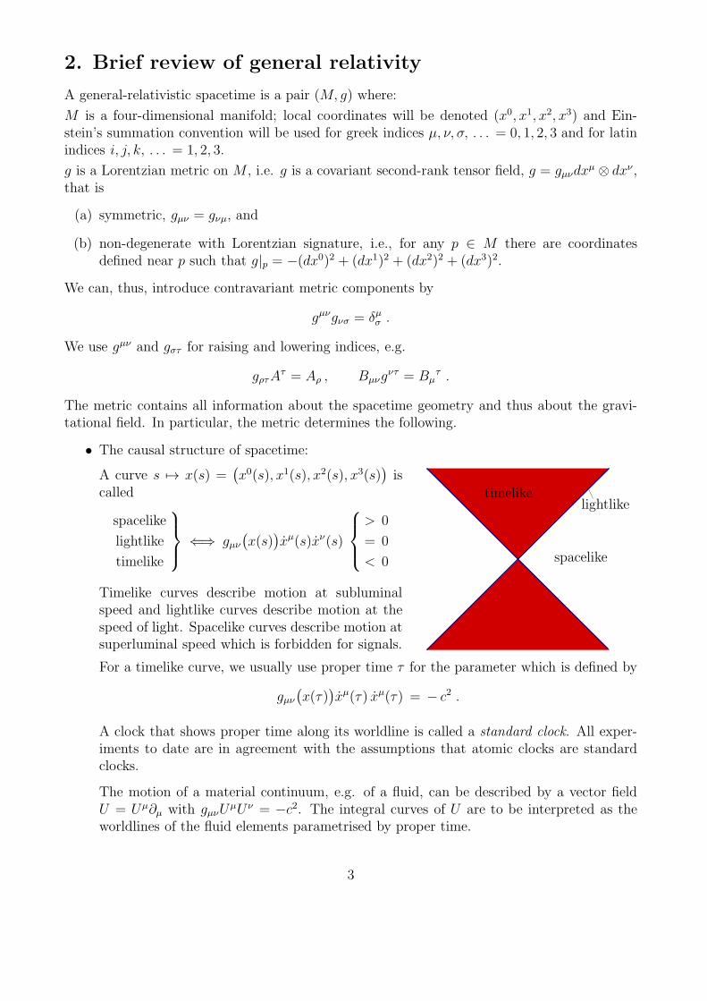
• The causal structure of spacetime:
A curve s 7→ x(s) =(
x0(s), x1(s), x2(s), x3(s))
iscalled
spacelike
lightlike
timelike
⇐⇒ gµν(
x(s))
xµ(s)xν(s)
> 0
= 0
< 0
Timelike curves describe motion at subluminalspeed and lightlike curves describe motion at thespeed of light. Spacelike curves describe motion atsuperluminal speed which is forbidden for signals.
timelikelightlike
spacelike
For a timelike curve, we usually use proper time τ for the parameter which is defined by
gµν(
x(τ))
xµ(τ) xµ(τ) = − c2 .
A clock that shows proper time along its worldline is called a standard clock. All exper-iments to date are in agreement with the assumptions that atomic clocks are standardclocks.
The motion of a material continuum, e.g. of a fluid, can be described by a vector fieldU = Uµ∂µ with gµνU
µUν = −c2. The integral curves of U are to be interpreted as theworldlines of the fluid elements parametrised by proper time.
3

• The geodesics:
By definition, the geodesics are the solutions to the Euler-Lagrange equations
d
ds
∂L(x, x)
∂xµ−
∂L(x, x)
∂xµ= 0
of the Lagrangian
L(
x, x)
=1
2gµν(x)x
µxν .
These Euler-Lagrange equations take the form
xµ + Γµ
νσ(x)xν xσ = 0
where
Γµ
νσ =1
2gµτ
(
∂νgτσ + ∂σgτν − ∂τgνσ)
are the so-called Christoffel symbols.
The Lagrangian L(x, x) is constant along a geodesic (see Worksheet 1), so we can speakof timelike, lightlike and spacelike geodesics. Timelike geodesics (L < 0) are to be inter-preted as the worldlines of freely falling particles, and lightlike geodesics (L = 0) are tobe interpreted as light rays.
The Christoffel symbols define a covariant derivative that makes tensor fields into tensorfields, e.g.
∇νUµ = ∂νU
µ + Γµ
ντUτ ,
∇νAµ = ∂νAµ − Γρ
νµAρ .
In Minkowski spacetime (i.e., in the “flat” spacetime of special relativity), we can choosecoordinates such that gµν = ηµν on the whole spacetime, where we have used the standardabbreviation (ηµν) = diag(−1, 1, 1, 1). In this coordinate system, the Christoffel symbolsobviously vanish. Conversely, vanishing of the Christoffel symbols on an open neigh-bourhood implies that the gµν are constants; one can then perform a linear coordinatetransformation such that gµν = ηµν .
• The curvature:
The Riemannian curvature tensor is defined, in coordinate notation, by
Rτ
µνσ = ∂µΓτ
νσ − ∂νΓτ
µσ + Γρ
νσΓτ
µρ − Γρ
µσΓτ
νρ .
This defines, indeed, a tensor field, i.e., if Rτµνσ vanishes in one coordinate system, then
it vanishes in any coordinate system. The condition Rτµνσ = 0 is true if and only if there
is a local coordinate system, around any one point, such that gµν = ηµν and Γµνσ = 0 on
the domain of the coordinate system.
The curvature tensor determines the relative motion of neighbouring geodesics: If X =Xµ∂µ is a vector field whose integral curves are geodesics, and if J = Jν∂ν connectsneighbouring integral curves of X (i.e., if the Lie bracket between X and J vanishes),then the equation of geodesic deviation or Jacobi equation holds:
4

(
Xµ∇µ
)(
Xν∇ν
)
Jσ = Rσ
µνρXµJνXρ .
If the integral curves of X are timelike, theycan be interpreted as worldlines of freelyfalling particles. In this case the curvatureterm in the Jacobi equation gives the tidal
force produced by the gravitational field.
If the integral curves of X are lightlike, theycan be interpreted as light rays. In this casethe curvature term in the Jacobi equationdetermines the influence of the gravitationalfield on the shapes of light bundles.
X
J
• Einstein’s field equation:
The fundamental equation that relates the spacetime metric (i.e., the gravitational field)to the distribution of energy is Einstein’s field equation:
Rµν −R
2gµν + Λgµν = κTµν
where
– Rµν = Rσµσν is the Ricci tensor ;
– R = Rµνgµν is the Ricci scalar ;
– Tµν is the energy-momentum tensor which gives the energy density TµνUµUν for any
observer field with 4-velocity Uµ normalised to gµνUµUν = −c2;
– Λ is the cosmological constant;
– κ is Einstein’s gravitational constant which is related to Newton’s gravitational con-stant G through κ = 8πG/c4.
Einstein’s field equation can be justified in the following way: One looks for an equationof the form (Dg)µν = Tµν where D is a differential operator acting on the metric. Onewants to have Dg satisfying the following two properties:
(A) Dg contains partial derivatives of the metric up to second order.
(B) ∇µ(Dg)µν = 0.
Condition (A) is motivated by analogy to the Newtonian theory: The Poisson equationis a second-order differential equation for the Newtonian gravitational potential φ, andthe metric is viewed as the general-relativistic analogue to φ . Condition (B) is motivatedin the following way: For a closed system, in special relativity the energy-momentumtensor field satisfies the conservation law ∂µTµν = 0 in inertial coordinates. By the ruleof minimal coupling, in general relativity the energy-momentum tensor field of a closedsystem should satisfy ∇µTµν = 0. For consistency, the same property has to hold for theleft-hand side of the desired equation.
5

D. Lovelock has shown in 1972 that these two conditions (A) and (B) are satisfied if andonly if Dg is of the form
(Dg)µν =1
κ
(
Rµν −R
2gµν + Λgµν
)
with some constants Λ and κ, i.e., if and only if the desired equation has indeed the formof Einstein’s field equation.
For vacuum (Tµν = 0), Einstein’s field equation reads
Rµν −R
2gµν + Λgµν = 0 .
By contraction with gµν this implies R = 4Λ, so the vacuum field equation reduces to
Rµν = Λgµν
Present-day cosmological observations suggest that we live in a universe with a positivecosmological constant whose value is Λ ≈ (1026m)−2 ≈ (1016ly)−2. As the diameter ofour galaxy is approximately 105ly, for any distance d within our galaxy the quantityd2Λ < 10−22 is negligibly small. As a consequence, the Λ term can be safely ignored forconsiderations inside our galaxy. Then the vacuum field equation takes the very compactform
Rµν = 0
which, however, is a complicated system of ten non-linear second-order partial differentialequations for the ten independent components of the metric.
Gravitational waves travelling through empty space are wavelike solutions of the equationRµν = 0.
6

3. Linearised field equation around flat spacetime
In 1916 Einstein predicted the existence of gravitational waves, based on his linearised vacuumfield equation. In 1918 he derived his famous quadrupole formula which relates emitted gravi-tational waves to the quadrupole moment of the source. In Chapters 3, 4 and 5 we will reviewthis early work on gravitational waves which is based on the linearised Einstein theory aroundflat spacetime. As a consequence, the results are true only for gravitational waves whose am-plitudes are small. We will see that, to within this approximation, the theory of gravitationalwaves is very similar to the theory of electromagnetic waves.We consider a spacetime metric gµν that takes, in appropriate coordinates, the form
gµν = ηµν + hµν .
Here ηµν denotes the Minkowski metric, i.e., the spacetime metric of special relativity, in inertialcoordinates,
(ηµν) = diag(−1, 1, 1, 1) ,
and the hµν are assumed to be so small that all expressions can be linearised with respect to thehµν and their derivatives ∂σhµν . In particular, it is our goal to linearise Einstein’s field equationwith respect to the hµν and their derivatives. This gives a valid approximation of Einstein’stheory of gravity if the spacetime is very close to the spacetime of special relativity.
Our assumptions fix the coordinate system up to transformations of the form
xµ 7→ xµ = aµ + Λµνxν + fµ(x) (C)
where (Λµν) is a Lorentz transformation, ΛµνΛρσηµρ = ηνσ, and the fµ are small of first order.
We agree that, in this chapter, greek indices are lowered and raised with ηµν and ηµν , respec-tively. Here ηµν is defined by
ηµνηνσ = δµσ .
We writeh := hµν η
µν = hµµ = hνν .
Then the inverse metric gνρis of the form
gνρ = ηνρ − hνρ .
Proof:(
ηµν + hµν) (
ηνρ − hνρ)
= ηµνηνρ + hµνη
νρ − ηµνhνρ + . . . = δρµ + hµ
ρ − hµρ =
δρµ , where the ellipses stand for a quadratic term that is to be neglected, according to ourassumptions.
We will now derive the linearised field equation. As a first step, we have to calculate theChristoffel symbols. We find
Γρµν =1
2gρσ
(
∂µgσν + ∂νgσµ − ∂σgµν)
=1
2ηρσ
(
∂µhσν + ∂νhσµ − ∂σhµν)
+ . . .
Thereupon, we can calculate the components of the Ricci tensor:.
Rµν = ∂µΓρρν − ∂ρΓ
ρµν + . . . =
=1
2ηρσ ∂µ
(
∂ρhσν + ∂νhσρ − ∂σhρν
)
−1
2ηρσ ∂ρ
(
∂µhσν + ∂νhσµ − ∂σhµν
)
=
7

=1
2
(
∂µ∂νh − ∂µ∂ρhρν − ∂σ∂νhσµ + hµν
)
.
Here, denotes the wave operator (d’Alembert operator) that is formed with the Minkowskimetric,
= ηµν∂µ∂ν = ∂ν∂ν .
From the last expression we can calculate the scalar curvature:
R = gµνRµν = ηµνRµν + . . . =1
2ηµν
(
∂µ∂νh − ∂µ∂ρhρν − ∂σ∂νhσµ + hµν
)
=1
2
(
h − ∂ν∂ρhρν − ∂σ∂µhσµ + h)
= h − ∂σ∂µhσµ .
Hence, the linearised version of Einstein’s field equation (without a cosmological constant)
2Rµν − Rgµν = 2 κTµν , κ =8πG
c4
reads
∂µ∂νh − ∂µ∂ρhρν − ∂σ∂νhσµ + hµν − ηµν
(
h − ∂σ∂τhστ)
= 2 κTµν . (∗)
This is a system of linear partial differential equations of second order for the hµν . It can berewritten in a more convenient form after substituting for hµν the quantity
γµν = hµν −h
2ηµν .
As the relation between hµν and γµν is linear, our assumptions are equivalent to saying thatwe linearise all equations with respect to the γµν and the ∂ργµν . In order to express the hµν interms of the γµν , we calculate the trace,
γ := ηµνγµν = h −1
24 h = −h ,
hµν = γµν −γ
2ηµν .
Upon inserting this expression into the linearised field equation (∗), we find
−∂µ∂νγ − ∂µ∂ργρν +
1
2ηρν∂µ∂
ργ − ∂σ∂νγσµ +1
2ησµ ∂
σ∂νγ +
+γµν −1
2ηµν γ − ηµν
(
− γ − ∂σ∂τγστ +
1
2ηστ∂
σ∂τγ)
= 2 κTµν ,
γµν − ∂µ∂ργρν − ∂ν∂
ργρµ + ηµν ∂σ∂τγστ = 2 κTµν . (∗∗)
This equation can be simplified further by a coordinate transformation (C) with aµ = 0 andΛµν = δµν ,
xµ 7→ xµ + fµ(x)
where the fµ are of first order. For such a coordinate transformation, we have obviously
dxµ 7→ dxµ + ∂ρfµdxρ
8

and thus∂σ 7→ ∂σ − ∂σf
τ∂τ .
Proof:(
dxµ + ∂ρfµdxρ
) (
∂σ − ∂σfτ∂τ
)
= dxµ(∂σ) + ∂ρfµdxρ(∂σ) − ∂σf
τdxµ(∂τ ) + . . . =δσµ + ∂ρf
µδρσ − ∂σfτδµτ .
With the help of these equations, we can now calculate how the gµν , the hµν , and the γµν behaveunder such a coordinate transformation:
gµν = g(
∂µ, ∂ν)
7→ g(
∂µ − ∂µfτ∂τ , ∂ν − ∂νf
σ∂σ)
= gµν − ∂µfτgτν − ∂νf
σgµσ ,
hµν = gµν − ηµν 7→ gµν − ∂µfτgτν − ∂νf
σgµσ − ηµν = hµν − ∂µfτητν − ∂νf
σηµσ + . . .
γµν = hµν −1
2ηµνh 7→ hµν − ∂µfν − ∂νfµ −
1
2ηµν
(
h− 2∂τfτ)
= γµν − ∂µfν − ∂νfµ + ηµν∂τfτ .
For the divergence of γµν , which occurs three times in (∗∗), this gives the following transfor-mation behaviour:
∂µγµν 7→ ∂µγµν − ∂µ∂µfν −∂µ∂νfµ +ηµν∂µ∂τf
τ = ∂µγµν −fν .
This shows that, if it is possible to choose the fν such that
fν = ∂µγµν ,
then ∂µγµν is transformed to zero. Such a choice is, indeed, possible as the wave equation onMinkowski spacetime,
fν = Φν ,
has solutions for any Φν . This is well-known from electrodynamics. (Particular solutions arethe retarded potentials, see below.)
We have thus shown that, by an appropriate coordinate transformation, we can put the lin-earised field equation (∗∗) into the following form:
γµν = 2 κTµν .
Now the γµν have to satisfy the additional condition
∂µγµν = 0
which is known as the Hilbert gauge. (Some other authors call it the Einstein gauge, thedeDonder gauge, or the Fock gauge.) The transformation of γµν under a change of coordinatesis analogous to a gauge transformation of the four-potential Aµ in electrodynamics. Even afterimposing the Hilbert gauge condition, there is still the freedom to make coordinate transforma-tions (C) with fµ = 0. In particular, the theory is invariant under Lorentz transformations.
9

The linearised Einstein theory is aLorentz invariant theory of the grav-itational field on Minkowski space-time. It is very similar to Maxwell’svacuum electrodynamics, which is a(linear) Lorentz invariant theory ofelectromagnetic fields on Minkowskispacetime. Of course, one has tokeep in mind that the linearised Ein-stein theory is only an approxima-tion; an exact Lorentz invariant the-ory of gravity on Minkowski space-time cannot be formulated. Einsteinand others tried this, without suc-cess, for several years before generalrelativity came into existence.
lin. Einstein theory electrodynamics
γµν Aµ
Tµν Jµ
Hilbert gauge ∂µγµν = 0 Lorenz gauge ∂µAµ = 0
γµν = −2κTµν Aµ = µ−1
0 Jµ
The table illustrates the analogy. Here “electrodynamics” stands for “electrodynamics onMinkowski spacetime in vacuum, Gµν = µ−1
0 Fµν”.
4. Gravitational waves in the linearised theory around flat spacetime
In this section we consider the linearised vacuum field equation in the Hilbert gauge,
γµν = 0 , ∂µγµν = 0 .
In analogy to the electrodynamical theory, we can write the general solution as a superpositionof plane harmonic waves. In our case, any such plane harmonic wave is of the form
γµν(x) = Re
Aµνeikρx
ρ
with a real wave covector kρ and a complex amplitude Aµν = Aνµ.Such a plane harmonic wave satisfies the linearised vacuum field equation if and only if
0 = ηστ∂σ∂τγµν(x) = Re
ηστAµνikσikτeikρx
ρ
.
This holds for all x, with (Aµν) 6= (0), if and only if
ηστkσkτ = 0 .
In other words, (k0, k1, k2, k3) has to be a lightlike covector with respect to the Minkowskimetric. This result can be interpreted as saying that, to within the linearised Einstein theory,gravitational waves propagate on Minkowski spacetime at the speed c, just as electromagneticwaves in vacuum.
10
Our plane harmonic wave satisfies the Hilbert gauge condition if and only if
0 = ηµτ∂τγµν(x) = Re
ηµτAµνikτeikρx
ρ
which is true, for all x = (x0, x1, x2, x3), if and only if
kµAµν = 0 (H) .
For a given kµ, the Hilbert gauge condition restricts the possible values of the amplitude Aµν ,i.e., it restricts the possible polarisation states of the gravitational wave. For electromagneticwaves, it is well known that there are two polarisation states (“left-handed and right-handed”,or “linear in x-direction and linear in y-direction”) from which all possible polarisation statescan be formed by way of superposition. We will see that also for gravitational waves there aretwo independent polarisation states; however, they are of a different geometric nature whichhas its origin in the fact that γµν has two indices while the electromagnetic four-potential Aµ
has only one.In order to find all possible polarisation states of a gravitational wave, we begin by counting theindependent components of the amplitude: The Aµν form a (4×4)-matrix which has 16 entries.As Aµν = Aνµ, only 10 of them are independent; the Hilbert gauge condition (H) consists of4 scalar equations, so one might think that there are 6 independent components and thus sixindependent polarisation states. This, however, is wrong. The reason is that we can imposeadditional conditions onto the amplitudes, even after the Hilbert gauge has been chosen: TheHilbert gauge condition is preserved if we make a coordinate transformation of the form
xµ 7→ xµ + fµ(x) mit fµ = 0 .
We can use this freedom to impose additional conditions onto the amplitudes Aµν .
Claim: Assume we have a plane-harmonic-wave solution
γµν(x) = Re
Aµνeikρx
ρ
of the linearised vacuum field equation in the Hilbert gauge. Let (uµ) be a constant four-velocityvector, ηµνu
µuν = − c2 . Then we can make a coordinate transformation such that the Hilbertgauge condition is preserved and such that
uµAµν = 0 , (T1)
ηµνAµν = 0 , (T2)
in the new coordinates (TT gauge, transverse-traceless gauge).
Proof: We perform a coordinate transformation
xµ 7→ xµ + fµ(x) , fµ(x) = Re
i Cµeikρxρ
with the wave covector (kρ) from our plane-harmonic-wave solution and with some complexcoefficients Cµ. Then we have fµ = 0, i.e., the Hilbert gauge condition is satisfied in the newcoordinates as well. We want to choose the Cµ such that in the new coordinates (T1) and (T2)hold true. As a first step, we calculate how the amplitudes Aµν transform.
11

We start out from the transformation behaviour of the γµν which was calculated above,
γµν 7→ γµν − ∂µfν − ∂νfµ + ηµν∂ρfρ ,
hence
Re
Aµνeikρx
ρ
7→ Re(
Aµν − i i kµCν − i i kνCµ + ηµνi i kρCρ)
eikρxρ
,
Aµν 7→ Aµν + kµCν + kνCµ − ηµν kρCρ .
We want to choose the Cµ such that the equations
0 = uµ(
Aµν + kµCν + kνCµ − ηµν kρCρ)
, (T1)
0 = ηµν(
Aµν + kµCν + kνCµ − ηµν kρCρ)
= ηµν Aµν − 2 kρCρ (T2)
hold. To demonstrate that such a choice is possible, we choose the coordinates such that
(
uµ)
=
c000
.
This can be done by a Lorentz transformation which, as a linear coordinate transformation,preserves all the relevant properties of the coordinate system. Then the spatial part of thedesired condition (T1) reads:
(T1) for ν = j : A0j + k0Cj + kjC0 = 0 ⇐⇒ Cj = − k−1
0 (A0j + kjC0) .
These equations show that the Cj are determined by C0. We will now check if the temporalpart of (T1) gives any restriction on C0.
(T1) for ν = 0 : A00 + 2 k0C0 + ηρσ kρCσ = 0 ⇐⇒
A00 + 2 k0C0 − k0C0 + ηij ki Cj = 0 ⇐⇒
A00 + k0C0 − ηij ki k−1
0
(
A0j + kjC0
)
= 0 ⇐⇒
A00 + k0C0 − ηij ki k−1
0 A0j + η00 k0k0 k−1
0 C0 = 0 ⇐⇒
− k0A00 + ηij kiA0j = 0 ⇐⇒
ηµνkµA0ν = 0 .
12

This is precisely the Hilbert gauge condition (H) that is satisfied by assumption. We have thusfound that (T1) fixes the Cj in terms of C0 but leaves C0 arbitrary.
We now turn to the second desired condition (T2).
(T2) : ηµν Aµν + 2 k0C0 − 2 ηij kiCj = 0 ⇐⇒
Aµµ + 2 k0C0 + 2 ηij ki k
−1
0
(
A0j + kjC0
)
= 0 ⇐⇒
Aµµ + 2 k0C0 + 2 ηij ki k
−1
0 A0j − 2 η00 k0k−1
0 k0 C0 = 0 ⇐⇒
Aµµ + 4 k0C0 + 2 ηij ki k
−1
0 A0j = 0 ⇐⇒
C0 =−Aµ
µ k0 − 2 ηij kiA0j
4 k20
.
If we choose C0 according to this equation, and then the Cj as required above, (T1) and (T2)are indeed satisfied in the new coordinates.
In the TT gauge we have γ = 0 and thus hµν = γµν . As a consequence, the metric is of theform
gµν = ηµν + γµν , γµν = Re
Aµνeikρx
ρ
and the amplitudes are restricted by the conditions
kµAµν = 0 , uµAµν = 0 , ηµνAµν = 0 .
If we choose the coordinates such that
(
uµ)
=
c000
,(
kρ)
=
ω/c00
ω/c
which can be achieved by a Lorentz transformation, the amplitudes Aµν satisfy
(H) 0 = kµAµν =ω
c(A0ν + A3ν) ,
(T1) 0 = uµAµν = cA0ν ,
(T2) 0 = ηµν Aµν = −A00 + A11 + A22 + A33
in the TT gauge. In this representation, there are only two non-zero components of Aµν ,
A11 = −A22 =: A+ =∣
∣A+
∣
∣ eiϕ ,
A12 = A21 =: A× =∣
∣A×
∣
∣ eiψ .
The fact that only the 1- and the 2-components are non-zero demonstrates that gravitationalwaves are transverse. There are only two independent polarisation states, the plus mode (+)and the cross mode (×).
13

For the physical interpretation of these two modes we need the following result.
Claim: The x0-lines, i.e. the worldlines xµ(τ) with xµ(τ) = uµ, are geodesics.
Proof: From xµ(τ) = uµ we find xµ(τ) = 0 . The Christoffel symbols read
Γµνσ =
1
2gµτ
(∂νgτσ + ∂σgτν − ∂τgνσ
)=
=1
2ηµτ
(∂νγτσ + ∂σγτν − ∂τγνσ
)=
=1
2ηµτ Re
(i kν Aτσ + i kσ Aτν − i kτ Aνσ
)eikρx
ρ .
Hence
xµ + Γµνσ x
ν xν = 0 +1
2ηµτ Re
(i kν Aτσ u
σ
︸ ︷︷ ︸
=0
uν + i kσ Aτν uν
︸ ︷︷ ︸
=0
uσ− i kτ Aνσ uσ
︸ ︷︷ ︸
=0
uν)eikρx
ρ = 0 .
In other words, the x0-lines are the worldlinesof freely falling particles. For any such particlethe (x1, x2, x3)-coordinates remain constant. Thisdoes, of course, not mean that the gravitationalwave has no effect on freely falling particles. Thedistance, as it is measured with the metric, be-tween neighbouring x0-lines is not at all constant.We calculate the square of the distance betweenthe x0-line at the spatial origin (0, 0, 0) and aneighbouring x0-line at (x1, x2, x3) for the case thatthe xi are so small that the metric can be viewedas constant between 0 and xi.
gij(x0, 0, 0, 0) (xi − 0) (xj − 0) =
x0
xi
=(ηij + γij(x
0, 0, 0, 0))xi xj = δij x
i xj + ReAijx
ixjeik0x0
=
= δij xi xj + Re
A+
((x1)2 − (x2)2
)e−iωt
+ Re
2A× x
1 x2e−iωt
=
= δij xi xj +
∣∣A+
∣∣((x1)2 − (x2)2
)cos
(ϕ− ωt
)+ 2
∣∣A×
∣∣ x1 x2 cos
(ψ − ωt
).
The last equation demonstrates what happens to particles that are arranged on a small sphericalshell and then released to free fall: Both the plus mode and the cross mode of the gravitationalwave produce a time-periodic elliptic deformation in the plane perpendicular to the propagationdirection. For the plus mode, the principal axes of the ellipse coincide with coordinate axes,for the cross mode they are rotated by 45 degrees. This explains the origin of the names “plusmode” and “cross mode”.
14

Plus mode (A+ 6= 0 , A× = 0):
x1
x2
ω t = ϕ
x1
x2
ω t = ϕ + π
x1
x2
ω t = ϕ + 2 π
Cross mode (A+ = 0 , A× 6= 0):
x1
x2
ω t = ψ
x1
x2
ω t = ψ + π
x1
x2
ω t = ψ + 2 π
The motion of test paticles under the influence of a gravitational wave can also be derivedas a solution of a differential equation. We will derive this differential equation, which is aspecification to the situation at hand of the Jacobi equation, in Worksheet 2. It will show thatthe “driving force” that generates the change of distances between neighbouring free particlesis the curvature tensor.
We have found, as our main result, that a gravitational wave produces a change of the distancesbetween freely falling particles in the plane perpendicular to the propagation direction. Thereare two types of gravitational wave detectors that try to measure this effect :
• Resonant bar detectors: The first gravitational wave detectors of this type were de-veloped by J. Weber in the 1960s. They were aluminium cylinders of about 1.5 m length.A gravitational wave of an appropriate frequency would excite a resonant oscillation ofsuch a cylinder. With the uprise of laser interferometric gravitational wave detectors, thebar detectors have lost their relevance. However, some of them are still used.
15

• Laser interferometric gravitational wave detectors: They are Michelson interfero-meters with an effective arm length of a few hundred meters at least. An incominggravitational wave would influence the distance between the mirrors and also the path ofthe light beam inside the interferometer. Both effects produce a change in the interferencepattern. Several such detectors are in operation since the early 2000s, e.g. GEO600 (nearHannover, the effective arm length is 600 meters) and LIGO (USA, three interferometersat two sites, the effective arm length is 2 kilometers and 4 kilometers, respectively). Aspace-borne interferometer (originally called LISA and planned with 5 million kilometersarm length) might be launched around 2034.
We will discuss both types of gravitational wave detectors in greater detail below.
As an aside, we mention that the wave equation for γµν and its solutions in the TT gauge area possible starting point for quantising the gravitational field. The resulting quanta, calledgravitons, have spin 2. This is related to the transformation behaviour of the solutions in theTT gauge under spatial rotations about the propagation direction. The latter will be calculatedin Worksheet 3.
5. Generation of gravitational waves
We will now discuss what sort of sources would produce a gravitational wave. We will see that,in the far-field approximation, the gravitational wave field is determined by the second time-derivative of the quadrupole moment of the source. In other words, gravitational radiationpredominantly is quadrupole radiation. By contrast, it is well known that electromagneticradiation predominantly is dipole radiation.
5.1 The far-field approximation of a gravitational wave
We consider the linearised field equation in the Hilbert gauge,
γµν = 2 κT µν , ∂µγµν = 0 .
For given Tµν , the general solution to this inhomogeneous wave equation is the general solutionto the homogeneous wave equation (superposition of plane harmonic waves) plus a particu-lar solution to the inhomogeneous equation. Such a particular solution can be written downimmediately by analogy with the retarded potentials from electrodynamics:
γµν(ct, ~r
)=
1
4 π
∫
R3
2 κT µν(c t − |~r ′ − ~r | , ~r ′
)d3~r ′
|~r ′ − ~r |. (RP)
Here and in the following we write
x0 = c t , (x1, x2, x3) = ~r , r = |~r |
and d3~r ′ is the volume element with respect to the primed coordinates, d3~r ′ = dx′1 dx′2 dx′3 .By differentiating twice one easily verifies that the γµν from (RP) satisfy, indeed, the equationγµν = 2 κT µν .
16

The general solution to the inhomogeneous wave equation is given by adding an arbitrarysuperposition of plane-harmonic waves that satisfy the homogeneous equation, see Chapter 4.If there are no waves coming in from infinity, (RP) alone gives the physically correct solution.We will now discuss this solution far away from the sources. To that end, we assume that T µν
is different from zero only in a compact region of space. We can then surround this regionby a sphere KR of radius R around the origin, such that T µν = 0 outside of KR and on theboundary. We are interested in the field γµν at a point ~r with |~r | ≫ R .
~r
~r ′
T µν 6= 0
T µν = 0Rϑ
KR
Then
|~r ′ − ~r | =
√(~r ′ − ~r
)·(~r ′ − ~r
)=
√
~r ′ · ~r ′ + ~r · ~r − 2~r ′ · ~r =
=
√
r′2 + r2 − 2 r′ r cosϑ = r
√
1 − 2r′
rcosϑ +
r′2
r2= r
(1 + O(r′/r)
).
Inserting the result into (RP) yields
γµν(ct, ~r
)=
κ
2 π
∫
R3
T µν(c t − r
(1 +O(r′/r)
), ~r ′
)d3~r ′
r(1 +O(r′/r)
) .
If r ≫ R, the O(r′/r)-terms can be neglected, as r′ ≤ R on the whole domain of integration.This is known as the far-field approximation,
γµν(ct, ~r
)=
κ
2 π r
∫
R3
T µν(c t − r , ~r ′
)d3~r ′ . (FF )
In this approximation, the γµν depend on ~r only in terms of its modulus r = |~r |, i.e., thewave fronts are spheres, r = constant. As the radii of these spheres are large, they can beapproximated as planes on a sufficiently small neighbourhood of any point ~r. This means that,on any such neighbourhood, our gravitational wave resembles a plane wave of the type we havestudied in Chapter 4.
17

We will now investigate which properties of the source determine the γij in the far-field ap-proximation. To that end we introduce the multipole moments of the source. They are de-fined in analogy to electrodynamics, with the charge density replaced by the energy densityT00 = −T0
0 = T 00.
M(t) =
∫
KR
T 00(ct, ~r
)d3~r (monopole moment) ,
Dk(t) =
∫
KR
T 00(ct, ~r
)xk d3~r (dipole moment) ,
Qkℓ(t) =
∫
KR
T 00(ct, ~r
)xk xℓ d3~r (quadrupole moment) ,
. . .
Note that each quadrupole moment is determined by its trace-free part and the quadrupolemoments of lower order. For this reason, some authors define the multipole moments as thetrace-free parts of our moments.
We calculate the first and second time derivative of the quadrupole moments. To that end, weneed to know that, because of the Hilbert gauge condition,
∂µTµν =
1
2 κ∂µ γµν =
1
2 κ ∂µγ
µν = 0 .
We find
d
dtQkℓ(t) =
∫
KR
c ∂0T00(ct, ~r ) xk xℓ d3~r = − c
∫
KR
∂iTi0(ct, ~r ) xk xℓ d3~r =
= − c
∫
KR
(
∂i(T i0(ct, ~r ) xk xℓ
)− T i0(ct, ~r ) δki x
ℓ − T i0(ct, ~r ) xk δℓi
)
d3~r .
The first integral can be rewritten, with the Gauss theorem, as a surface integral over theboundary ∂KR of KR,
∫
KR
∂i(T i0(ct, ~r ) xk xℓ
)d3~r =
∫
∂KR
T i0(ct, ~r ) xk xℓdfi
where dfi is the surface element on ∂KR. As the sphere KR surrounds all sources, T µν is equalto zero on ∂KR, so the last integral vanishes. Hence
d
dtQkℓ(t) = c
∫
KR
(T k0(ct, ~r ) xℓ + T ℓ0(ct, ~r ) xk
)d3~r .
Analogously we calculate the second derivative.
18

d2
dt2Qkℓ(t) = c2
∫
KR
(
∂0Tk0(ct, ~r ) xℓ + ∂0T
ℓ0(ct, ~r ) xk)
d3~r =
= c2∫
KR
(
− ∂iTki(ct, ~r ) xℓ − ∂iT
ℓi(ct, ~r ) xk)
d3~r =
= c2∫
KR
(
− ∂i(T ki(ct, ~r ) xℓ
)+ T ki(ct, ~r ) δℓi − ∂i
(T ℓi(ct, ~r ) xk
)+ T ℓi(ct, ~r ) δki
)
d3~r =
= 0 + c2∫
KR
T kℓ(ct, ~r ) d3~r − 0 + c2∫
KR
T ℓk(ct, ~r ) d3~r .
As T kℓ = T ℓk, this can be rewritten as
d2
dt2Qkℓ(t) == 2 c2
∫
KR
T kℓ(ct, ~r ′ ) d3~r ′
where we have renamed the integration variable. Upon inserting this result into (FF) we findthat, in the far-field approximation,
γkℓ(ct, ~r ) =κ
2 π r
∫
R3
T kℓ(
c t − r, ~r ′
)
d3~r ′ =κ
2 π r
1
2 c2d2Qkℓ
dt2
(
t −r
c
)
.
If Einstein’s gravitational constant is expressed with the help of Newton’s gravitational con-stant, κ = 4πG/c4, the result reads
γkℓ(ct, ~r ) =G
c6 r
d2Qkℓ
dt2
(
t −r
c
)
.
The only property of the source that a gravitational wave detector can measure far away fromthe source is, thus, the second time derivative of the quadrupole moment at a retarded time.In this sense, gravitational radiation is quadrupole radiation, while electromagnetic radiationis dipole radiation. Roughly speaking, the difference has its origin in the fact that γµν and T µν
have two indices while the analogous quantities Aµ and Jµ in electrodynamics have only oneindex.
A time-dependent monopole moment (e.g. a pulsating spherically symmetric star) does not pro-duce gravitational radiation. This is a consequence of Birkhoff’s theorem acoording to whichthe spacetime outside of a spherically symmetric source is always the static Schwarzschild solu-tion. We have now seen that, moreover, a time-dependent dipole moment does not produce anygravitational radiation in the far-field approximation. We need a time-dependent quadrupolemoment. As an exmaple, we may think of a periodically squashed ball. Also, two massesorbiting their barycentre have a time-dependent quadrupole moment.
19

Note that, according to our results on the preceding page, only the spatial components γkℓ aregiven by the second time derivative of the quadrupole moment. What about the time-time andthe time-space components?
Claim: For a source T µν that is confined to a finite sphere for all times, in the far-field thecomponents γi0 vanish and the component γ00 is time-independent and falls off like r−1.
Proof: See Worksheet 4.
For this reason, the components γ0µ give no contribution to the radiation field in the far zone.In the next section we calculate the loss of energy of a system that emits gravitational waves.
5.2 Energy and momentum of a gravitational wave
The question of how to assign energy and momentum to a gravitational wave is conceptuallysubtle. According to general relativity, the gravitational field is not to be considered as a fieldon the spacetime, it is coded in the geometry of the spacetime itself. The energy-momentumtensor on the right-hand side of Einstein’s field equation comprises everything with the exception
of the gravitational field. An energy-momentum tensor of the gravitational field is not definedand cannot be defined. This is in correspondence with the equivalence principle according towhich the gravitational field (coded in the Christoffel symbols which act as the “guiding field”for test particles and light) can be transformed to zero in any one point. As a non-zero tensor isnon-zero in any coordinates, this is a clear indication that something like an energy-momentumtensor of the gravitational field cannot exist.
However, a (non-tensorial) quantity that describes energy and momentum of a gravitationalfield can be defined with respect to a background metric. We assume that we have a spacetimemetric which takes, in the chosen coordinates the form
gµν(x) = ηµν + hµν(x) .
For the time being, we do not assume that the hµν are small. The coordinates are then fixedup to Lorentz transformations
xµ 7→ xµ = Λµνx
ν , ΛµσΛ
ντηµν = ηστ . (LT)
The Ricci tensor of the metric g is then of the form
Rµν(h) = R(1)µν (h) +R(2)
µν (h) + . . .
where R(n)µν (h) comprises all terms of nth order in the hρσ and their first and second derivatives.
Similarly, the Einstein tensor is of the form
Gµν(h) = Rµν(h) −1
2gµν g
ρσRρσ(h) = G(1)µν (h) +G(2)
µν (h) + . . .
where
G(1)µν (h) = R(1)
µν (h)−1
2ηµνη
ρσR(1)ρσ (h) ,
20
G(2)µν (h) = R(2)
µν (h)−1
2ηµνη
ρσR(2)ρσ (h)−
1
2hµνη
ρσR(1)ρσ (h) +
1
2ηµνh
ρσR(1)ρσ (h) ,
and so on. Here we have used that gρσ = ηρσ − hρσ + . . .
We assume that our metric gµν = ηµν + hµν satisfies Einstein’s field equation, with a sourceterm Tµν , exactly,
Gµν(h) = κTµν .
We rewrite this equation by keeping only the first-order terms on the left-hand side and shiftingall higher-order terms to the right-hand side,
G(1)µν (h) = κ
(Tµν + tµν
), (FEB)
tµν = −1
κ
(Gµν(h)−G(1)
µν (h))= −
1
κ
(G(2)
µν (h) + . . .)
According to (FEB), h satisfies the linearised field equation with a source term Tµν + tµν . Ofcourse, this is still the same Einstein equation which is non-linear. We have just renamed thenon-linear terms into tµν and re-interpreted them as additional sources.
The tµν are not the components of a tensor; it is easy to check that the G(1)µν and hence the tµν
transform as tensor components under Lorentz transformations (LT), but not under arbitrarycoordinate changes. tµν is called the energy-momentum pseudotensor of the gravitational field.
The following observation is crucial.
Claim: The combined source term Tµν = tµν satisfies the continuity equation
∂µ(Tµν + tµν
). (CL)
Proof: See Worksheet 4.
This conservation law is not a covariant equation. It holds only in the special coordinates inwhich our background metric has components ηµν . However, it really gives rise to a conservationlaw in integral form if integrated over a spacetime region (“the change of the energy contentinside a spatial volume equals the energy flux over the boundary”). By contrast, the covariantdivergence law ∇µTµν , which is satisfied by our true matter source, is only a conservation lawin “infinitesimally small regions”; it does not give rise to a conservation law in integral form.
If our matter source loses energy, exactly the same amount of energy must be carried awayin the form of gravitational waves according to the conservation law (CL). This is the way inwhich the observations of the Hulse-Taylor pulsar are interpreted (which will be discussed indetail below): One observes that the system loses energy and one concludes that this energy iscaried away in the form of gravitational waves.
Linearising the field equation with respect to the hµν and their derivatives is tantamount tosetting tµν equal to zero. In this approximation, Tµν alone satisfies the conservation law (CL).We have to go at least to the second order if we want to have a non-trivial tµν . In the second-order theory, we write the metric as
gµν = ηµν + h(1)µν + h(2)
µν + . . .
where h(1)µν is a solution to the linearised field equation. The h
(1)µν are small of first order while
the h(2)µν are small of second order. In other words, terms linear in the h
(2)µν are treated at the
same footing as terms quadratic in the h(1)µν .
21

Expanding both sides of (FEB) up to second order results in
G(1)µν (h
(1) + h(2)) = κ(Tµν + tµν
),
tµν = −1
κG(2)
µν (h(1)) .
In other words, we get the energy-momentum pseudotensor of a gravitational field in its lowestnon-trivial approximation if we insert the corresponding solution to the linearised field equationh(1)ρσ into G
(2)µν . We will now carry out this calculation for a plane-harmonic wave of the kind we
have considered in Chapter 4. On the basis of this result, we will then determine the powerthat is radiated away from a source that is confined to a finite sphere, as we have consideredin Section 5.1.
As before, we raise and lower indices with ηµν and ηµν , respectively. We need to calculate
R(2)µν (h) which is a bit tedious. We begin with the Christoffel symbols
Γρµν =
1
2gρσ
(∂µgσν + ∂νgσµ − ∂σgµν
)=
1
2
(ηρσ − hρσ + . . .
)(∂µhσν + ∂νhσµ − ∂σhµν
).
The Ricci tensor is
Rµν = Rρµρν = ∂µΓ
ρρν − ∂ρΓ
ρµν + Γρ
σµΓσρν − Γρ
σρΓσµν ,
hence
R(2)µν = −
1
2∂µ(hρσ(
∂ρhσν + ∂νhσρ −
∂σhρν)
)+
1
2∂ρ(hρσ(∂µhσν + ∂νhσµ − ∂σhµν)
)
+1
4ηρτ
(∂σhτµ + ∂µhτσ − ∂τhσµ
)ησλ
(∂ρhλν + ∂νhλρ − ∂λhρν
)
−1
4ηρτ
(∂σhτρ +
∂ρhτσ −
∂τhσρ
)ησλ
(∂µhλν + ∂νhλµ − ∂λhµν
)
We want to calculate the time-space components
t0j = −1
κG
(2)0j (h
(1))
for a plane-harmonic wave in the TT gauge,
h(1)µν (x) = γµν(x) = Re
Aµνe
ikρxρ
where kµkµ = 0 , γµν(x)k
ν = 0 , γµµ(x) = 0 , γ0ν(x) = 0 . Up to a factor −c, the time-space
components t0j give the energy current density sj with respect to an observer whose four-velocityuρ is tangent to the x0 lines,
sj = −uρtρj = −u0t0j = −ctoj .
We find
κ t0j = R(2)0j (h
(1)) + 0 + 0 + 0 =1
2∂0(γρσ∂jγσρ
)−
1
2∂ρ(γρσ∂0hσj
)
22
−1
4ηρτ∂0γτση
σλ(
∂ργλj + ∂jγλρ −
∂λγρj)+
1
4ηρτ∂σγτρ︸ ︷︷ ︸
= ∂σγτ τ =0
ησλ∂0γλj
=1
2∂0γ
ρσ∂jγσρ +1
2γρσ∂0∂jγσρ − 0 −
1
2γρσ∂ρ∂0γσj︸ ︷︷ ︸
∼γρσkρ =0
−1
4∂0γ
ρλ∂jγλρ
=1
4∂0γ
ρσ∂jγσρ +1
2γρσ∂0∂jγσρ =
1
4∂0γ
kℓ∂jγkℓ +1
2γkℓ∂0∂jγkℓ
=1
4Re
Akℓik0e
ikρxρRe
Akℓikje
ikρxρ
+1
2Re
Akℓeikρx
ρRe
−Akℓk0kje
ikρxρ
.
We introduce the covector
nj =kj
k0
which is parallel to the spatial wave covektor kj and normalised, because
njnj =
kjkj
k20
=kρk
ρ − k0k0
k20
=0 + k2
0
k20
= 1 .
Hence
κ t0j =k0kj
4Re
Akℓ i eikρx
ρRe
Akℓ i e
ikρxρ
−k0kj
2Re
Akℓ eikρx
ρRe
Akℓ e
ikρxρ
=k20nj
16
(Akℓ i eikρx
ρ
− Akℓ i e−ikρxρ)(
Akℓ i eikρx
ρ
− Akℓ i e−ikρxρ)
−k20nj
8
(Akℓ e
ikρxρ
+ Akℓ e−ikρxρ)(
Akℓ eikρxρ
+ Akℓ e−ikρxρ)
= −3k2
0nj
16
(
AkℓAkℓ e2ikρxρ
+ AkℓAkℓ e−2ikρxρ
)
−k20nj
8AkℓAkℓ
= −3k2
0nj
8
(
ReAkℓAkℓ
cos
(2kρx
ρ)− Im
AkℓAkℓ
sin
(2kρx
ρ))
−k20nj
8Akℓ Akℓ
where an overbar means complex conjugation. The first two terms, which are proportional tocos(2kρx
ρ) = cos(2kixi − 2ωt) and sin(2kρx
ρ) = sin(2kixi − 2ωt), respectively, vary periodically
with time around zero. If we consider the time-average, denoted by 〈·〉, they drop out. Thetime-averaged energy current density of a plane-harmonic gravitational wave in the TT gaugeis
〈sj〉 = − c 〈t0j〉 =c k2
0nj
8κAkℓAkℓ .
This expression can be rewritten as
〈sj〉 =c nj
4 κ
⟨∂0γ
kℓ∂0γkℓ⟩
(EC)
as follows from comparison with
⟨∂0γ
kℓ∂0γkℓ⟩=
⟨Re
Akℓ i k0 e
ikρxρRe
Akℓ i k0 e
ikσxσ⟩
=k20
4
⟨(Akℓ i eikρx
ρ
− Akℓ i e−ikρxρ)(
Akℓ i eikσx
σ
− Akℓ i e−ikσx
σ)⟩
=k20
2Akℓ Akℓ .
23

We now turn back to the situation of an energy-momentum tensor field which has supportinside a sphere of radius R, for all time, see picture on p.17. We know from Section 5.1 thatthe solution to the linearised field equation satisfies, in the far zone,
γkℓ(ct, ~r ) =κ
4 π r c2d2Qkℓ
dt2
(
t −r
c
)
.
This γkℓ, which satisfies the Hilbert gauge condition but not in general the TT gauge condition,can be viewed, in a sufficiently small neighbourhood of any one point in the far zone, as asuperposition of plane-harmonic waves propagating in the direction nj , where nj is the unitvector in the radial direction. However, we cannot apply (EC) directly for calculating thetime-averaged energy current of this gravitational wave, because (EC) holds only for a plane-harmonic wave in the TT gauge. We have to project onto the transverse-traceless part of γkℓ
first.
Projecting onto the transverse part means projecting onto the orthocomplement of nj , i.e.applying the projection operator
Pij = δ
ji − nin
j
which satisfies the projection property
PijPj
k =(δji − nin
j)(δkj − njn
k)= δki − nin
k −nin
k +nin
k = Pik
and the symmetry property P rs = P sr. After applying this projection operator we have tosubtract the trace to get the transverse-traceless part of γkℓ,
γTTkℓ = Pk
iPℓjγij −
1
2PkℓP
rsPriPs
jγij = PkiPℓ
jγij −1
2PkℓP
ijγij .
For applying (EC) to our gravitational field in the far zone we need to calculate
∂0γTTkℓ∂0γ
TTkℓ = ∂0
(P kmP ℓnγmn −
1
2P kℓPmnγmn
)∂0(Pk
rPℓsγrs −
1
2PkℓP
rsγrs)
=(P kmP ℓnPk
rPℓs −
1
2P kmP ℓnPkℓP
rs −1
2P kℓPmnPk
rPℓs +
1
4P kℓPmnPkℓP
rs)∂0γmn∂0γrs
=(PmrP ns −
1
2PmnP rs −
1
2P rsPmn +
1
4Pk
kPmnP rs)∂0γmn∂0γrs
=(PmrP ns−PmnP rs+
1
4(δkk − nkn
k)︸ ︷︷ ︸
=2
PmnP rs)∂0γmn∂0γrs =
(PmrP ns−
1
2PmnP rs
)∂0γmn∂0γrs
=((δmr − nmnr)(δns − nnns)−
1
2(δmn − nmnn)(δrs − nrns)
)∂0γmn∂0γrs
=(
δmrδns −δmnδrs
2− 2δmrnnns + δmnnrns +
nmnnnrns
2
)
∂0γmn∂0γrs
Note that nj is the unit vector in radial direction, so it depends on ~r but not on t. Time-averaging over an appropriate interval yields
⟨∂0γ
TTkℓ∂0γTTkℓ
⟩=
(
δmrδns −δmnδrs
2− 2δmrnnns + δmnnrns +
nmnnnrns
2
)
〈∂0γmn∂0γrs〉 .
24

This gives us the time-averaged energy current density
〈sj〉 (ct, ~r) =c nj
4κ
(
δmrδns − δmnδrs
2− 2δmrnnns + δmnnrns +
nmnnnrns
2
)
〈∂0γmn∂0γrs〉 (ct, ~r) .
With
∂0γkℓ(ct, ~r ) = ∂0
κ
4 π r c2d2Qkℓ
dt2
(
t − r
c
)
=κ
4 π r c3d3Qkℓ
dt3
(
t − r
c
)
we find〈sj〉 (ct, ~r)
=κnj
64π2r2c5
(
δmrδns − δmnδrs
2− 2δmrnnns + δmnnrns +
nmnnnrns
2
)⟨d3Qmn
dt3d3Qrs
dt3
⟩(
t− r
c
)
.
This equation holds at any point ~r in the far zone where nj denotes the unit vector in radialdirection at this point. We can integrate this equation over a sphere of radius r(≫ R) to getthe radiated power (energy per time) that passes through this sphere
P (t, r) =
2π∫
0
π∫
0
〈sj〉 (ct, ~r)r2njsin ϑ dϑ dϕ =
2π∫
0
π∫
0
(
δmrδns−δmnδrs
2−2δmrnnns+δmnnrns+
nmnnnrns
2
)κnjr2njsinϑ dϑ dϕ
64π2r2c5
⟨d3Qmn
dt3d3Qrs
dt3
⟩(
t−r
c
)
.
Claim:2π∫
0
π∫
0
nknℓsinϑ dϑ dϕ =4π
3δkℓ and
2π∫
0
π∫
0
nknℓnrnssinϑ dϑ dϕ =4π
15(δkℓδrs+δkrδℓs+δksδrℓ).
Proof: We calculate for all (ξ1, ξ2, ξ3) ∈ R3,
π∫
0
2π∫
0
ξiξjninjsinϑ dϕ dϑ =
∫ π
0
∫ 2π
0
(ξ1sinϑ cosϕ+ ξ2sin ϑ sinϕ+ ξ3cos ϑ
)2sin ϑ dϕ dϑ
= ξ21
π∫
0
sin3ϑ dϑ
2π∫
0
cos2ϕdϕ
︸ ︷︷ ︸
=π
+ ξ22
π∫
0
sin3ϑ dϑ
2π∫
0
sin2ϕdϕ
︸ ︷︷ ︸
=π
+ ξ23
π∫
0
cos2ϑ sin ϑ dϑ
2π∫
0
dϕ
︸ ︷︷ ︸
=2π
.
For all other terms the ϕ integration gives zero. Hence
π∫
0
2π∫
0
ξiξjninjdϕ dϑ =
(π ξ21 + π ξ22
)π∫
0
sin3ϑ dϑ
︸ ︷︷ ︸
=4/3
+ 2 π ξ23
π∫
0
cos2ϑ sin ϑ dϑ
︸ ︷︷ ︸
=2/3
=4π
3
(ξ21 + ξ22 + ξ23
)=
4π
3δijξiξj .
25

Similarly,
π∫
0
2π∫
0
ξiξjξkξℓninjnknℓsin ϑ dϕ dϑ =
∫ π
0
∫ 2π
0
(ξ1sin ϑ cosϕ+ ξ2sinϑ sinϕ+ ξ3cosϑ
)4sinϑ dϕ dϑ
= ξ41
π∫
0
sin5ϑ dϑ
2π∫
0
cos4ϕdϕ
︸ ︷︷ ︸
=3π/4
+ ξ42
π∫
0
sin5ϑ dϑ
2π∫
0
sin4ϕdϕ
︸ ︷︷ ︸
=3π/4
+ 6ξ21ξ22
π∫
0
sin5ϑ
2π∫
0
cos2ϕ sin2ϕdϕ
︸ ︷︷ ︸
=π/4
+6ξ21ξ23
π∫
0
cos2ϑ sin3ϑ dϑ
2π∫
0
cos2ϕdϕ
︸ ︷︷ ︸
=π
+6ξ22ξ23
π∫
0
cos2ϑ sin3ϑ dϑ
2π∫
0
sin2ϕdϕ
︸ ︷︷ ︸
=π
+ξ43
π∫
0
cos4ϑ sin ϑ dϑ
2π∫
0
dϕ
︸ ︷︷ ︸
=2π
=3π
4
(ξ41 + ξ42 + 2ξ21ξ
22
)π∫
0
sin5ϑ dϑ
︸ ︷︷ ︸
=16/15
+ 6π(ξ21 + ξ22)ξ23
π∫
0
cos2ϑ sin3ϑ dϑ
︸ ︷︷ ︸
=4/15
+ 2 π ξ43
π∫
0
cos4ϑ sin ϑ dϑ
︸ ︷︷ ︸
=2/5
=4π
5
(ξ21 + ξ22 + ξ23
)2=
4π
5δijδkℓξiξjξkξℓ .
Symmetrisation of the coefficients gives the desired result.
HenceP (t, r) =
κ
16πc5
(
δmrδns−δmnδrs
2−2δmrδns
3+δmnδrs
3+δmnδrs + δmrδns + δmsδrn
30
)⟨d3Qmn
dt3d3Qrs
dt3
⟩(
t−r
c
)
=κ
16πc5
(2δmrδns
5− 2δmnδrs
15
)⟨d3Qmn
dt3d3Qrs
dt3
⟩(
t− r
c
)
=κ
40πc5
(
δmrδns − δmnδrs
3
)⟨d3Qmn
dt3d3Qrs
dt3
⟩(
t− r
c
)
=κ
40πc5
⟨d3Qmn
dt3d3Qmn
dt3− 1
3
d3Qmm
dt3d3Qr
r
dt3
⟩(
t− r
c
)
.
This can be rewritten more conveniently if we introduce the reduced quadrupole moment Qkℓ
which is defined as the trace-free part of Qkℓ,
Qkℓ = Qkℓ −1
3δkℓQj
j .
Then the energy flux through the sphere of radius r reads
P (t, r) =κ
40πc5
⟨d3
dt3
(
Qmn +1
3δmnQk
k) d3
dt3
(
Qmn +1
3δmnQℓ
ℓ)
− 1
3
d3Qmm
dt3d3Qr
r
dt3
⟩(
t− r
c
)
26

=κ
40πc5
⟨d3Qmn
dt3d3Qmn
dt3+ 0 + 0 +
1
93d3Qk
k
dt3d3Qℓ
ℓ
dt3−1
3
d3Qkk
dt3d3Qℓ
ℓ
dt3
⟩(
t− r
c
)
which eventually gives us Einstein’s quadrupole formula
P (t, r) =κ
40πc5
⟨d3Qmn
dt3d3Qmn
dt3
⟩(
t− r
c
)
.
This formula allows us to calculate the power that is radiated away by a time-dependent mattersource. If we want to apply this formula, we need to know the reduced quadrupole moment ofthe source. Note that this is the energy quadrupole moment,
Qkℓ = Qkℓ −1
3δkℓQj
j ,
Qkℓ(t) =
∫
R3
T00(ct, ~r)xkxℓd3~r
which requires to know the energy density T00. The latter contains the whole energy contentof the source which is difficult to determine. For slowly moving bodies the biggest contributionto the energy density comes from the mass density µ(ct, ~r). As long as the source involves onlymotions that are slow in comparison to the speed of light, we can write
T00(ct, ~r) ≈ c2µ(ct, ~r) .
as a valid approximation. We can then replace the reduced energy quadrupole moment Qkℓ bythe reduced mass quadrupole moment
Ikℓ = Ikℓ −1
3δkℓIj
j ,
Ikℓ(t) =
∫
R3
µ(ct, ~r)xkxℓd3~r
With the aproximationQkℓ ≈ c2 Ikℓ
Einstein’s quadrupole formula reads
P (t, r) =κ
40 π c
⟨d3Imn
dt3d3Imn
dt3
⟩(
t− r
c
)
or, with κ = 8πG/c4,
P (t, r) =G
5 c5
⟨d3Imn
dt3d3Imn
dt3
⟩(
t− r
c
)
.
This is the form in which the formula is usually applied. In this version, the quadrupole formulainvolves the following approximations.
• The energy-momentum pseudotensor was calculated only to within second order (which isthe lowest non-trivial order); the solution to the field equation that is needed to calculatethis order is a first-order solution, i.e., a solution to the linearised field equation.
27

• The formula holds in the far zone, i.e., it gives the energy flux per time through a sphereof radius r which is big in comparison to the radius R of the sphere to which the mattersource Tµν is confined.
• The formula is based on the assumption that all motions inside the source are slow incomparison to the speed of light.
In addition, the formula involves a time-averaging over an interval that covers the periods ofall Fourier components that contribute to the gravitational wave.
5.3 Gravitational waves from a binary source
We consider a binary system consisting of two masses M1 and M2 moving around each other.It is sufficient to describe the system at the Newtonian level, that is, to describe the motionof the two masses in terms of their Keplerian orbits. (We make later remarks about possibleeffects which are neglected herewith.)
The relative distance between the two masses is denoted by r. From the Kepler problem weknow that
r(ϕ) =R0
1 + e cosϕ, (K)
where R0 is the semi-latus rectum and e is the eccentricity of the orbit. The semi-major axisa and the semi-minor axis b of the orbit are given by
2a = r(0) + r(π) =R0
1 + e+
R0
1− e= 2
R0
1− e2
b =R0√1− e2
.
We first calculate the mass quadrupole tensor in the co-rotating system, that is, in the body-fixed coordinate system. Then we transform into the non-rotating observer system. At last,the third time-derivative of this mass quadrupole tensor has to be inserted into the radiationformula. From that we can calculate the change of the orbital parameters of the system due tothe loss of energy.
For the body-fixed coordinate system we choose as the origin the centre of mass. Then thedistances of the two masses from the centre of mass are given by
r1 = − M2
M1 +M2
r , r2 =M1
M1 +M2
r .
Consistency requires r = −r1+ r2 which is fulfilled. We call the direction of the line between themasses the 1-direction. The 2-direction is in the orbital plane and the 3-direction is orthogonalto the orbital plane.
Then the mass quadrupole tensor is diagonal, with
I1 = M1r21 +M2r
22 = M1
(
− M2
M1 +M2r
)2
+M2
(M1
M1 +M2r
)2
=M1M2
M1 +M2r2 .
28

The other components vanish. Thus, the mass quadrupole tensor is
I ′ =
I1 0 00 0 00 0 0
.
The traceless version of this mass quadrupole tensor is
I′ = I ′ − 1
3trI ′ 1 =
I1 0 00 0 00 0 0
− 1
3
I1 0 00 I1 00 0 I1
=1
3
2I1 0 00 −I1 00 0 −I1
.
This mass quadrupole tensor, given in the body-fixed coordinate system, has to be transformedto the non-rotating observer system. This has to be done by means of a rotation matrix for arotation around the 3-axis,
α =
cosϕ − sinϕ 0sinϕ cosϕ 00 0 1
.
In matrix form the mass quadrupole tensor is then given by
I = α I′ αT
=
cosϕ − sinϕ 0sinϕ cosϕ 00 0 1
1
3
2I1 0 00 −I1 00 0 −I1
cosϕ sinϕ 0− sinϕ cosϕ 0
0 0 1
=1
3
cosϕ − sinϕ 0sinϕ cosϕ 00 0 1
2I1 cosϕ 2I1 sinϕ 0I1 sinϕ −I1 cosϕ 0
0 0 −I1
=I13
2 cos2 ϕ− sin2 ϕ 3 cosϕ sinϕ 03 cosϕ sinϕ 2 sin2 ϕ− cos2 ϕ 0
0 0 −1
=I13
3 cos2 ϕ− 1 32sin(2ϕ) 0
32sin(2ϕ) −3 cos2 ϕ+ 2 00 0 −1
=I13
32(1− cos(2ϕ))− 1 3
2sin(2ϕ) 0
32sin(2ϕ) −3
2(1− cos(2ϕ)) + 2 0
0 0 −1
=I13
12
0 00 1
20
0 0 −1
+I12
− cos(2ϕ) sin(2ϕ) 0sin(2ϕ) cos(2ϕ) 0
0 0 0
,
which consists of a constant part and a part depending on the angle of rotation ϕ.
Instead of the angle of rotation ϕ one can introduce the mean anomaly M = ϕ − e sinϕwhich increases uniformly with time. The time derivative of ϕ can be expressed through theconstant angular momentum L = M1M2
M1+M2r2ϕ, that is, ϕ = (M1+M2)
M1M2
Lr2 , where r is given by (K).
Differentiating I three times requires some calculation, see Worksheet 5. In order to shorten
29

the calculations and to highlight the relevant effect of inspiralling we restrict here to a circularorbit, that is, to e = 0. In this case we have a constant r. From Kepler’s third law
4π2 r3
T 2= G(M1 +M2)
we obtain the angular frequency of the rotation of the binary system
Ω =2π
T=
√
G(M1 +M2)
r3
,
so thatϕ = Ωt .
We now calculate the power loss with the help of the quadrupole formula
P (t, r) =G
5c5
⟨
tr(...
I ·...
I
)⟩ (t− r
c
).
Recall that this formula gives the power that passes through a (big) sphere of radius r at timet. (Don’t confuse r = |~r |, the radius coordinate of the observer, with r, the distance of the twomasses.) In the case at hand, 〈 · 〉 denotes averaging over a period 2π/Ω.
We find
I = I1Ω
sin(2ϕ) cos(2ϕ) 0cos(2ϕ) − sin(2ϕ) 0
0 0 0
I = 2I1Ω2
cos(2ϕ) − sin(2ϕ) 0− sin(2ϕ) − cos(2ϕ) 0
0 0 0
...
I = 4I1Ω3
− sin(2ϕ) − cos(2ϕ) 0− cos(2ϕ) sin(2ϕ) 0
0 0 0
and
tr(...
I ·...
I
)
= (4I1Ω3)2tr
− sin(2ϕ) − cos(2ϕ) 0− cos(2ϕ) sin(2ϕ) 0
0 0 0
− sin(2ϕ) − cos(2ϕ) 0− cos(2ϕ) sin(2ϕ) 0
0 0 0
= (4I1Ω3)2tr
1 0 00 1 00 0 0
= 2(4I1Ω3)2 .
With this we obtain
P =G
5c52(4I1Ω
3)2 =G
5c532
M21M
22
(M1 +M2)2r4G
3(M1 +M2)3
r9
=32G4
5c5M2
1M22 (M1 +M2)
r5
.
30

P is the power radiated away by the binary system. Therefore, the binary system loses energy.During this process r decreases slowly with time. We have to insert r at the retarded time,r(t− r/c), to get the power that passes through a sphere of (big) radius r at time t.The energy in a binary system is given by
E =1
2
M1M2
(M1 +M2)v2 − GM1M2
r
.
For the circular orbit we obtain
E =1
2
M1M2
(M1 +M2)(Ωr)2 − GM1M2
r
=1
2
M1M2
(M1 +M2)
G(M1 +M2)
r3
r2 − GM1M2
r
= −1
2M1M2
G
r
so that the loss in energy can be described as
P = −dE
dt= −GM1M2
2r2dr
dt.
With the power P calculated above we obtain
dr
dt= −64G3
5c5M1M2(M1 +M2)
r3
.
We can rewrite this as
−A = const = r3r =
1
4
d
dtr4 .
Thereforer4 = A0 − 4At .
A0 is the fourth power of the initial radius r0 at t = 0. Then
r(t) =(r40 − 4At
) 1
4 = r0
(
1− 4A
r40
t
) 1
4
=: r0
(
1− t
tspiral
) 1
4
,
where
tspiral :=r40
4A=
5c5
256G3
r40
M1M2(M1 +M2)
is the time the system needs to inspiral completely.
It is clear that for a weaker gravitational coupling, that is, for a smaller G, the time for theinspiralling becomes larger. It is also interesting to see the velocity of light in the numerator.This means that for larger c, i.e., for approaching the nonrelativistic regime, also the inspiraltime becomes larger. Therefore gravitational radiation is not only a gravitational but also arelativistic effect. For typical values like Solar masses and distances of several Solar radii theinspiral time is of the order of billions of years.
In addition to the approximations on which the quadrupole formula is based, we have madea number of additional approximations. We add now some remarks on the limitations of ourmodel.
31

1. We assumed a circular orbit. The calculation with eccentric orbits is more involved, seeWorksheet 5.
2. We assumed the stars to be point particles. Stars are extended bodies and will be de-formed when they approach each other. So, during the last phase of the inspiralling thiswould lead to modifications of our result due to a shift of the centre of gravity and dueto additional couplings of the star with the gravity gradient.
3. Due to gravitomagnetic effects also the spin of stars will lead to modifications of theinspiralling.
We recall that the quadrupole formula is valid only to within the linearised theory of gravityand that it gives the power that passes through a sphere in the far zone. Using the massquadrupole tensor instead of the energy quadrupole tensor is justified unless the motion of thesource is highly relativistic. During the last phase of the inspiralling such highly relativisticeffects may contribute, in particular for merging black holes.
In Worksheet 5 we generalise the results of this section to the case of non-circular orbits. Inparticluar, we will derive formulas for the time-dependence of the semi-major axis a and of theperiod T . We will find that
a =2a2E
GM1M2
=−64M1M2G
3(M1 +M2)
5c5a3(1− e2)7/2
(
1 +73e2
24+
37e4
96
)
,
T
T=
−96M1M2G3(M1 +M2)
5c5a4(1− e2)7/2
(
1 +73e2
24+
37e4
96
)
.
As the masses are in the numerator and the semi-major axis is in the denominator, the lattereven with a power of 4, we see that a measurable effect can be expected only for compactbinaries, i.e., not for main sequence stars or planets, but for neutron stars or black holes. Inthe next section we will discuss how the predictions of general relativity have been verified withbinary pulsars, i.e., binaries where at least one partner is a rotating neutron star.
5.4 Indirect evidence for gravitational waves from binary pulsars
Before coming to binary pulsars, we will briefly recall what pulsars are and how they werediscovered.
Pulsars were discovered in 1967 by Jocelyn Bell, who is shown in Fig. 5.1, then a PhD studentin the group of Antony Hewish at Cambridge University. Fig. 5.2 shows Hewish in front of thedo-it-yourself radio telescope with which the discovery was made.
Fig. 5.1: from cwp.library.ucla.edu/
32

Fig. 5.2: from www.mrao.cam.ac.uk/
After having constructed the radio telescope, together with other students, with her own hands,Jocelyn Bell concentrated in her PhD work on the search for quasars with the scintillationmethod. The observation was often affected by interferences caused by terrestrial sources suchas cars. On 6 August 1967 Jocelyn Bell observed some “scruff”, as she later put it, that appearedto be different from these usual interferences, see Fig. 5.3. She discussed the observation withher supervisor. After having verified that the source remained fixed with respect to the stars itseemed certain that it was an astronomical object. Hewish and Bell decided to look at it moreclosely.
Fig. 5.3: from pulsar.ca.astro.it/
On 28 November 1967 Jocelyn Bell observed the mysterious object with a higher time resolution,see Fig. 5.4. It showed highly regularly pulses with a period of 1.337 seconds. It was seriouslydiscussed in the group whether the signal could come from an alien civilisation, and it was onlyhalf-jocular that the object was initially called LGM-1, with LGM standing for Little Green
Men. Later, the object was given the systematic name PSR B1919+21. Here PSR stands forPulsating Source of Radio emission, which was soon abbreviated as pulsar and the numbersgive the celestial coordinates of the source, a point in the constellation Vulpecula: 19h19m isthe right ascension and +21o is the declination; the letter B is added for coordinates referingto the epoch 1950 while a letter J is added for the epoch 2000.
Within a few weeks the Cambridge group found three more similar objects. In early 1968,they published their observations, see A. Hewish, J. Bell, J. Pilkington, P. Scott and R. Collins[“Observation of a rapidly pulsating radio source” Nature 217, 709 (1968)].
33

Fig. 5.4: from www.bbc.co.uk/
Passionate discussions started about the nature of the radiation. A majority, including Hewish,first thought that it might come from radial oscillations of a white dwarf. However, it turnedout that not even a white dwarf, let alone a main sequence star, could perform oscillationswith such a high frequency. After about a year, it was the prevailing opinion that the radiationcomes from a rotating neutron star. Thomas Gold was the first to suggest such a model in early1968 [T. Gold: “Rotating neutron stars as the Origin of the pulsating radio sources” Nature218, 731-732 (1968)], which was initially ridiculed by many astrophysicists. The idea was thatthe neutron star has a magnetic field that is not aligned with the rotation axis. Radiation isemitted in a cone around the magnetic field axis, and this cone rotates like the beacon of alighthouse. The observer registers a pulse whenever the cone hits the Earth. Neutron starshad been introduced, as a theoretical possibility, in 1934 by Walter Baade and Fritz Zwicky,but up to the discovery of pulsars there was no indication that they actually exist in Nature.An animation of the lighthouse model can be found in Section 2.1 of D. Lorimer [“Binaryand Millisecond Pulsars”, Living Rev. Relativity 11, (2008), http://www.livingreviews.org/lrr-2008-8].
Fig. 5.5: from en.wikipedia.org
Within a few years after the discovery of PSR B1919+21, several dozens of pulsars were found.14 of them are shown in the plaques that are on board the spacecraft Pioneer 10 and 11. Theywere launched in 1972 and 1973 and are the first spacecraft to leave the Solar system. Thepositions of the pulsars are shown, relative to the Earth, in the diagram in the left part of theplaque, see Fig. 5.5. This should tell an extraterrestrial civilisation where the spacecraft camefrom, in case that Pioneer 10 or 11 is intercepted by them.
The best known example of a pulsar is the neutron star at the centre of the Crab Nebula. It isthe remnant of a supernova that was observed from the Earth in 1054. It is also visible in theoptical and X-ray parts of the spectrum. There are also some pulsars that emit gamma rays,e.g. the Vela pulsar.
34

In 1974 Hewish received the Nobel Prize for the discovery of pulsars. Some people thoughtthat it would have been fair if Jocelyn Bell had shared the prize. By now more than 2000radio pulsars are known. Most of them are within our galaxy, but there are also a few in theMagellanic Clouds. The periods vary from a few milliseconds to about 10 seconds.
Fig. 5.6: from th.physik.uni-frankfurt.de/
After these remarks on pulsars in general, we turn now to binary pulsars. This term refersto binary systems in which at least one partner is a pulsar. About 10 % of all known pulsarshave a companion. The first binary pulsar, PSR B1913+16, was discovered in 1974. It wasagain the work of a PhD student and a supervisor, this time Russell Hulse and Joseph Taylorfrom Cornell University who are shown in Fig. 5.6. In contrast to the earlier story, both wereawarded the Nobel Prize in 1993.
Fig. 5.7: from en.wikipedia.org
The discovery was made with the 305-meter Arecibo radio telescope, see Fig. 5.7. The objectis a pulsar with a period of 59 milliseconds. Evidence for the existence of a companion, whichis dark and mute, came from the fact that the arrival time of the pulses varied periodically.Obviously, the pulsar is moving towards us, then away from us, then again towards us, and soon.
35

Fig. 5.8: from Hulse and Taylor, loc. cit.
The plot of the radial velocity in Fig. 5.8 is taken from the original paper by R.Hulse andJ. Taylor [“Discovery of a pulsar in a binary system” Astrophys. J. 195, L51 (1975)]. Aftercorrecting for the motion of the Earth, for dispersion in the intergalactic medium and for othereffects, Hulse and Taylor fitted the observed time dependence of the radial velocity to a Keplerorbit. There is a certain degeneracy, i.e., not all orbital elements can be uniquely determined,but the following parameters of the system were found. The numbers are taken, again, fromthe paper by Hulse and Taylor.
T 7.75 hourse 0.16
a1 sin i 1.0R⊙
(M2sin i )3
(M1 +M2)20.13M⊙
Here an index 1 stands for the pulsar and an index 2 stands for the invisible companion. iis the inclination angle. From the Newtonian analysis one cannot determine the individualmasses M1 and M2. However, this is possible with the help of relativistic corrections, usingthe post-Newtonian (PN) approximation. Roughly speaking, this is an expansion in powersof v/c. If relativistic effects are taken into account, in particular the transverse Doppler effectand the gravitational Doppler effect, the individual masses and all orbital parameters can bedetermined. The method, which was worked out by V. Brumberg, Y. Zeldovich, I. Novikovand N. Shakura [“Determination of the component masses and inclination of a binary systemcontaining a pulsar from relativistic effects”, Sov. Astr. Lett. 1, 2 (1975)], is sketched inStraumann’s book. One finds
M1 1.44M⊙
M2 1.39M⊙
i 45o
periastron shift 4.2 o/yr
36

At periastron, the separation of the two stars is only 1.1 Solar radii, at apastron it is 4.5 Solarradii. The companion is thought to be a neutron star as well. We do not know the radii of thetwo stars precisely, but typically neutron stars have radii in the order of 10 kilometers.
Already in the original Hulse-Taylor paper it is remarked that the system should be a highlypromising candidate for testing general relativity. In the above-mentioned paper by Brumberget al. it was noted that it could provide indirect evidence for the existence of gravitationalwaves: With the masses and the orbital elements known, one could check if the period Tdepends on time according to the formula derived from general relativity.
Fig. 5.9: From Taylor and Weisberg, loc. cit.
Such a dependence of T on time was reported by J. Taylor, L. Fowler and P. McCulloch[“Measurements of general relativistic effects in the binary pulsar PSR 1913+16” Nature 277,437 (1979)] and confirmed, on the basis of more data, by J. Taylor and J. Weisberg [“A new testof general relativity - Gravitational radiation and the binary pulsar PSR 1913+16” Astrophys.J. 253, 908 (1982)]. The plot in Fig. 5.9 is taken from the latter paper. It clearly shows thedecrease of the orbital period. The solid line gives the prediction according to general relativity,on the basis of the determined orbital parameters. In the course of time, the agreement betweenobservation and theory became even more impressive, see Fig. 5.10.
Fig. 5.10: from www.ast.cam.ac.uk
37
After the discovery of the Hulse-Taylor pulsar, several other binary pulsars were detected. Theyare used on a regular basis for testing general relativity and alternative theories of gravity. Upto now, general relativity has passed all tests with flying colours, whereas severe restrictionshave been found for many alternative theories.
In addition to the Hulse-Taylor pulsar, there are some other binary pulsars that deserve specialattention.
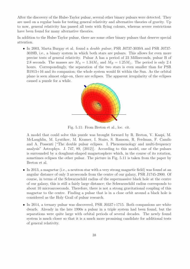
• In 2003, Marta Burgay et al. found a double pulsar, PSR J0737-3039A and PSR J0737-3039B, i.e., a binary system in which both stars are pulsars. This allows for even moreprecise tests of general relativity. Pulsar A has a period of 23 Milliseconds, pulsar B of2.8 seconds. The masses are MA = 1.34M⊙ and MB = 1.25M⊙. The period is only 2.4hours. Correspondingly, the separation of the two stars is even smaller than for PSRB1913+16 and its companion; the whole system would fit within the Sun. As the orbitalplane is seen almost edge-on, there are eclipses. The apparent irregularity of the eclipsescaused a puzzle for a while.
Fig. 5.11: From Breton et al., loc. cit.
A model that could solve this puzzle was brought forward by R. Breton, V. Kaspi, M.McLaughlin, M. Lyutikov, M. Kramer, I. Stairs, S. Ransom, R. Ferdman, F. Camiloand A. Possenti [“The double pulsar eclipses. I. Phenomenology and multi-frequencyanalysis” Astrophys. J. 747, 89, (2012)]. According to this model, one of the pulsarsis surrounded by a doughnut-shaped magnetosphere which, in the course of its rotation,sometimes eclipses the other pulsar. The picture in Fig. 5.11 is taken from the paper byBreton et al.
• In 2013, a magnetar (i.e., a neutron star with a very strong magnetic field) was found at anangular distance of only 3 arcseconds from the centre of our galaxy, PSR J1745-2900. Ofcourse, in terms of the Schwarzschild radius of the supermassive black hole at the centreof our galaxy, this is still a fairly large distance; the Schwarzschild radius corresponds toabout 10 microarcseconds. Therefore, there is not a strong gravitational coupling of thismagnetar to the centre. Finding a pulsar that is in a close orbit around a black hole isconsidered as the Holy Grail of pulsar research.
• In 2014, a ternary pulsar was discovered, PSR J0337+1715. Both companions are whitedwarfs. Already in the late 1990s a pulsar in a triple system had been found, but theseparations were quite large with orbital periods of several decades. The newly foundsystem is much closer so that it is a much more promising candidate for additional testsof general relativity.
38

6. Gravitational wave detectors
In the preceding chapter we have discussed the generation of gravitational waves. As the mostimportant results, we have found that, to within certain approximations, the gravitational fieldin the far zone is determined by the second time-derivative of the (mass) quadrupole tensorof the source and that the radiated power is determined by the third time-derivative of thisquadrupole tensor. In this chapter we will now introduce various types of gravitational wavedetectors that have been conceived and we will discuss what are the chances that actuallygravitational waves will be observed with them.
6.1 Resonant bar detectors
Resonant bar detectors are vibrating systems in which a gravitational wave would excite aresonant oscillation. The idea was brought forward in 1960 by Joseph Weber [“Detection andgeneration of gravitational waves”, Phys. Rev. 117, 306 (1960)]. A few years later, the firstresonant bar detectors constructed by Weber went into operation. Some more sophisticatedresonant bar detectors are still in use.
To explain the basic idea, we begin by considering the simplest vibrating system that can beused as a gravitational wave detector, namely two masses connected by a spring. This simpleexample is also treated in the first part of Weber’s 1960 paper and it is dicussed in fairly greatdetail in the book by Misner, Thorne and Wheeler.
We have to recall some of our earlier results. In Worksheet 2 we derived a differential equationfor the motion of freely falling particles under the influence of a gravitational wave,
d2yℓ(t)
c2dt2= Rℓ
0k0
(
ct,~0)
yk(t) , (J)
where the curvature tensor can be expressed as
Rℓ0k0
(
ct,~0)
=1
2∂20γ
ℓk
(
ct,~0)
.
Here γℓk is a plane-harmonic gravitational wave in the TT gauge, with the four-velocity uµ of
the chosen observer tangent to the x0-lines. The coordinates yk are chosen such that the freelyfalling particle at yk(t) has distance
√
yk(t)yk(t) from the freely falling particle at the origin.The differential equation is linearised with respect to yk(t), i.e., it is valid only as long as thisquantity is sufficiently small.
(J) is a version of the Jacobi equation (or equation of geodesic deviation). If looked at withNewtonian eyes, the right-hand side of (J) is to be interpreted as the gravitational force. Thesolutions to (J) give, for γℓ
k either a plus mode or a cross mode, the familiar patterns fromp.15.
We will now consider a particle with mass m that is acted on by an additional (i.e., non-gravitational) force f ℓ(t). Then we have to replace (J) with the equation of motion
d2yℓ(t)
dt2= c2Rℓ
0k0
(
ct,~0)
yk(t) +1
mf ℓ(t) .
39
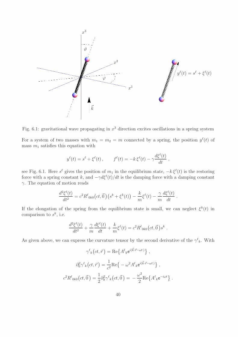
x1
x2
x3
ϑ
ϕ
~k
yℓ(t) = sℓ + ξℓ(t)
Fig. 6.1: gravitational wave propagating in x3 direction excites oscillations in a spring system
For a system of two masses with m1 = m2 = m connected by a spring, the position yℓ(t) ofmass m1 satisfies this equation with
yℓ(t) = sℓ + ξℓ(t) , f ℓ(t) = −k ξℓ(t)− γdξℓ(t)
dt,
see Fig. 6.1. Here sℓ gives the position of m1 in the equilibrium state, −k ξℓ(t) is the restoringforce with a spring constant k, and −γdξℓ(t)/dt is the damping force with a damping constantγ. The equation of motion reads
d2ξℓ(t)
dt2= c2Rℓ
0k0
(
ct,~0)(
sk + ξk(t))
−k
mξℓ(t)−
γ
m
dξℓ(t)
dt.
If the elongation of the spring from the equilibrium state is small, we can neglect ξk(t) incomparison to sk, i.e.
d2ξℓ(t)
dt2+
γ
m
dξℓ(t)
dt+
k
mξℓ(t) = c2Rℓ
0k0
(
ct,~0)
sk .
As given above, we can express the curvature tensor by the second derivative of the γℓk. With
γℓk
(
ct, ~r)
= Re
Aℓke
i(~k·~r−ωt )
,
∂20γ
ℓk
(
ct, ~r)
=1
c2Re
− ω2Aℓke
i(~k·~r−ωt )
,
c2Rℓ0k0
(
ct,~0)
=1
2∂20γ
ℓk
(
ct,~0)
= −ω2
2Re
Aℓke
−iωt
.
40

If we assume that the masses at the ends of the spring can be displaced only in the longitudinaldirection of the spring, we have
ξℓ(t) = ξ(t)sℓ
s,
where, according to Fig. 6.1,
(
sℓ)
= s
cosϕ sinϑsinϕ sinϑ
cos ϑ
,(
ξℓ(t))
= ξ(t)
cosϕ sinϑsinϕ sinϑ
cosϑ
.
Then the equation of motion reads
sℓ
s
(d2ξ(t)
dt2+
γ
m
dξ(t)
dt+
k
mξ(t)
)
= −ω2
2Re
Aℓks
ke−iωt
,
or, after multiplication with sℓ/s,
sℓsℓ
s2
(d2ξ(t)
dt2+
γ
m
dξ(t)
dt+
k
mξ(t)
)
= −ω2
2Re
Aℓks
k sℓse−iωt
.
We evaluate the right-hand side for a pure plus mode. The gravitational wave is assumed topropagate in the x3 direction, as indicated in Fig. 6.1 by the wave vector ~k. We find
(
Aℓk
)
=
A+ 0 00 −A+ 00 0 0
,
sℓAℓks
k = s
cosϕ sinϑsinϕ sinϑ
cosϑ
·
A+ 0 00 −A+ 00 0 0
s
cosϕ sinϑsinϕ sinϑ
cosϑ
= s2
cosϕ sinϑsinϕ sinϑ
cos ϑ
·
A+cosϕ sinϑ−A+sinϕ sinϑ
0
= s2A+
(
cos2ϕ− sin2ϕ)
sin2ϑ = s2A+cos(2ϕ)sin2ϑ .
This gives us the equation of motion in its final form,
d2ξ(t)
dt2+
γ
m
dξ(t)
dt+
k
mξ(t) = −
sω2
2cos(2ϕ)sin2ϑRe
A+e−iωt
,
which is the equation of a one-dimensional damped harmonic oscillator with a driving force.
Solving this equation is an elementary text-book matter. The general solution to the inhomo-geneous ODE is the general solution of the homogeneous ODE plus a particular solution to theinhomogeneous ODE.
To solve the homogeneous ODE,
d2ξ(t)
dt2+
γ
m
dξ(t)
dt+
k
mξ(t) = 0 ,
we insert the ansatzξ(t) = C e
κt .
41

This gives us
C eκt(
κ2 +γ κ
m+
k κ
m
)
= 0 ,
hence
κ1/2 = −γ
2m±
√
γ2
4m2−
k
m.
As long as the damping is undercritical,
0 <k
m−
γ2
4m2=: ω2
0 ,
we haveκ1/2 = −
γ
2m± i ω0 ,
and the general solution to the homogeneous equation is
ξhom = C1eκ1t + C2e
κ2t = e−γt/(2m)
(
C1eiω0t + C2e
−iω0t)
.
C1 and C2 are determined by initial conditions. Whatever the initial conditions are, the solutiondies down in the course of time.
We have now to find one particular solution to the inhomogeneous equation
d2ξ(t)
dt2+
γ
m
dξ(t)
dt+
k
mξ(t) = −
s ω2
2cos(2ϕ) sin2ϑRe
A+ e−iωt
.
With the ansatzξ(t) = Re
a e−iωt
we get
Re
a e−iωt(
− ω2 −iωγ
m+
k
m
)
= −s ω2
2cos(2ϕ) sin2ϑRe
A+ e−iωt
,
Re
e−iωt
(
a(
ω2 −k
m+
i ω γ
m
)
−s ω2A+
2cos(2ϕ) sin2ϑ
)
= 0 ,
a =s ω2A+cos(2ϕ) sin
2ϑ
ω2 −k
m+
i ω γ
m
.
Therefore, if we wait until the solution to the homogeneous equation has died down, the oscil-lation of our spring system driven by the gravitational wave is given by
ξ(t) = Re
a e−iωt
= s ω2cos(2ϕ) sin2ϑRe A+ e
−iωt
ω2 −k
m+
i ω γ
m
.
The amplitude
∣
∣a∣
∣ =s∣
∣A+
∣
∣
∣
∣cos(2ϕ)∣
∣ sin2ϑω2
∣
∣
∣ω2 −
k
m+
i ω γ
m
∣
∣
∣
=s∣
∣A+
∣
∣
∣
∣cos(2ϕ)∣
∣ sin2ϑω2
√
(
ω2 −k
m
)2
+ω2 γ2
m2
takes, as a function of ω, its maximum at the resonance frequency
ωres =k
m
( k
m−
γ2
4m2
)
−1/2
.
42
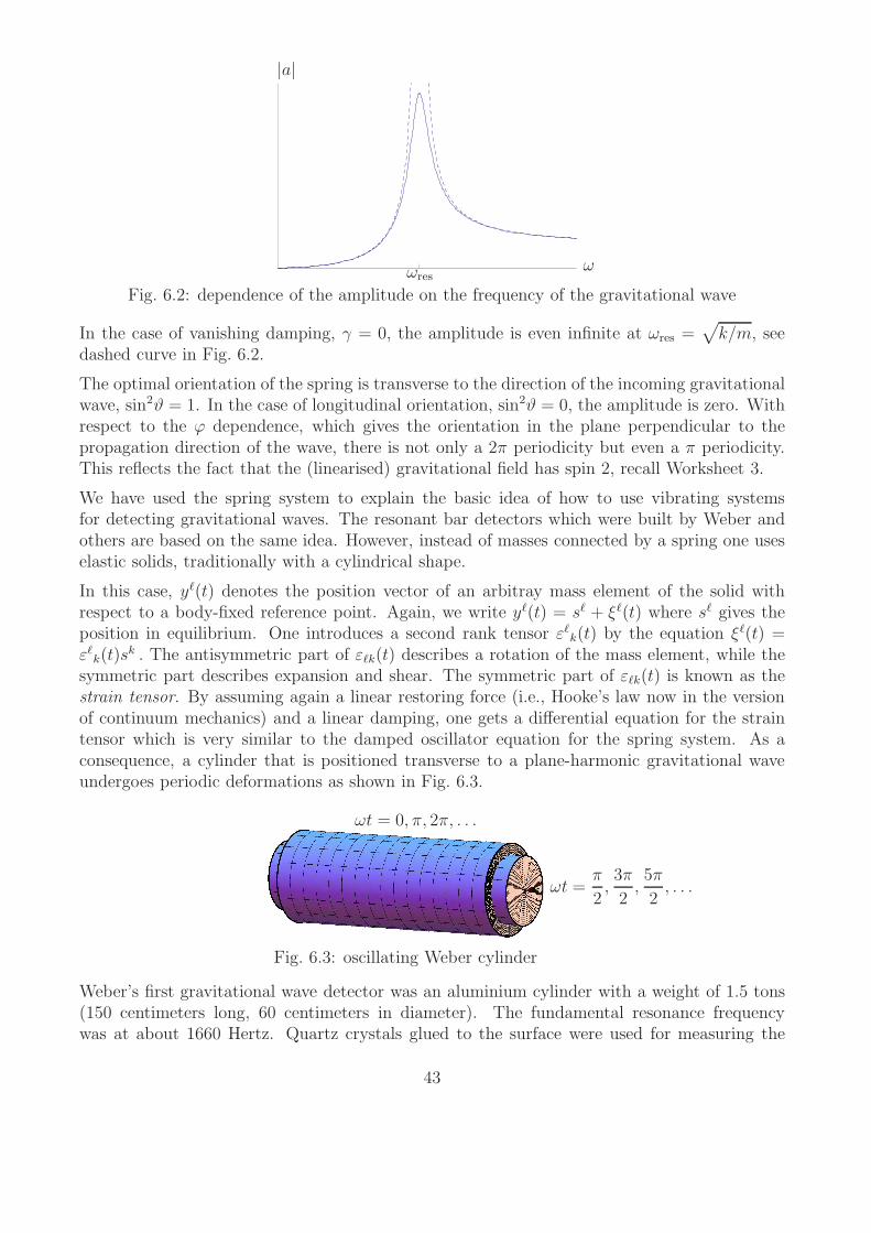
ω
|a|
ωres
Fig. 6.2: dependence of the amplitude on the frequency of the gravitational wave
In the case of vanishing damping, γ = 0, the amplitude is even infinite at ωres =√
k/m, seedashed curve in Fig. 6.2.
The optimal orientation of the spring is transverse to the direction of the incoming gravitationalwave, sin2ϑ = 1. In the case of longitudinal orientation, sin2ϑ = 0, the amplitude is zero. Withrespect to the ϕ dependence, which gives the orientation in the plane perpendicular to thepropagation direction of the wave, there is not only a 2π periodicity but even a π periodicity.This reflects the fact that the (linearised) gravitational field has spin 2, recall Worksheet 3.
We have used the spring system to explain the basic idea of how to use vibrating systemsfor detecting gravitational waves. The resonant bar detectors which were built by Weber andothers are based on the same idea. However, instead of masses connected by a spring one useselastic solids, traditionally with a cylindrical shape.
In this case, yℓ(t) denotes the position vector of an arbitray mass element of the solid withrespect to a body-fixed reference point. Again, we write yℓ(t) = sℓ + ξℓ(t) where sℓ gives theposition in equilibrium. One introduces a second rank tensor εℓk(t) by the equation ξℓ(t) =εℓk(t)s
k . The antisymmetric part of εℓk(t) describes a rotation of the mass element, while thesymmetric part describes expansion and shear. The symmetric part of εℓk(t) is known as thestrain tensor. By assuming again a linear restoring force (i.e., Hooke’s law now in the versionof continuum mechanics) and a linear damping, one gets a differential equation for the straintensor which is very similar to the damped oscillator equation for the spring system. As aconsequence, a cylinder that is positioned transverse to a plane-harmonic gravitational waveundergoes periodic deformations as shown in Fig. 6.3.
Fig. 6.3: oscillating Weber cylinder
ωt = 0, π, 2π, . . .
ωt =π
2,3π
2,5π
2, . . .
Weber’s first gravitational wave detector was an aluminium cylinder with a weight of 1.5 tons(150 centimeters long, 60 centimeters in diameter). The fundamental resonance frequencywas at about 1660 Hertz. Quartz crystals glued to the surface were used for measuring the
43

deformations; as quartz crystals are piezoelectric, they transform a strain into a voltage whichcan be measured, see Fig. 6.4.
Fig. 6.4: from Levine, loc. cit.
The early attempts to measure gravitational waves with the help of resonant bar detectors aredescribed in detail by J. Levine [“Early gravity-wave detection experiments”, Phys. perspect.6, 42 (2004)]. Fig. 6.5 shows Joe Weber working on a resonant bar detector.
Fig. 6.5: from physics.aps.org/
Weber operated his resonant bar detectors in pairs, searching for coincidences. In the beginning,he had two detectors on the campus of Maryland University, then he moved one of them toChicago. There was even an attempt to station a (smaller) bar detector on the Moon withthe Apollo 17 mission but the instrument malfunctioned. Weber claimed that he had foundsignificant statistical evidence for coincident events which he thought to be gravitational wavesignals. Nowadays there is agreement that his detectors were too crude to measure gravitationalwaves.
Joseph Weber died in the year 2000. By that time, attempts to detect gravitational waves hadshifted to interferometric methods, see next section. However, there are still a few resonant bardetectors in operation. Fig. 6.6 shows the AURIGA instrument, near Pisa in Italy, which is aresonant bar detector of the traditional cylindrical shape.
44

Fig. 6.6: from www.auriga.lnl.infn.it/
Fig. 6.7 shows the MiniGRAIL instrument at the Kamerlingh Onnes Institute in Leiden, Nether-lands. It has a spherical shape, so it can detect gravitational waves from all spatial directions.There is a similar instrument, named after the late physicist Mario Schenberg, in Brazil.
Fig. 6.7: from www.minigrail.nl/
While in the beginning Weber did his observations at room temperature, all modern resonantbar detectors are operated at a temperature of a few millikelvins to reduce thermal noise. Theycan detect waves only in a narrow frequency band around the resonance frequency which isabove or slightly below 1 kHz. Gravitational waves from the Hulse-Taylor pulsar, e.g., cannotbe detected with these instruments; this is not only because their sensitivity is too low butalso because they cannot detect gravitational waves of such a low frequency. (The revolutionperiod in the Hulse-Taylor binary is 7.75 hours, i.e. the frequency of the resulting gravitationalwaves is 2Ω = 4π/T ≈ 0.00045 Hz.) Spinning bumpy neutron stars could produce gravitationalwaves with a frequency close to 1 kHz, but their amplitude would probably be too low for beingdetected with resonant bar detectors. Therefore, the search with such instruments concentrateson burst sources.
45

6.2 Interferometric gravitational wave detectors
With the help of a Michelson interferometer, tiny distance changes can be measured. Theidea to use this well-known fact for the detection of gravitational waves came up in the early1960s. The first published paper on the subject was by M. Gerstenshtein and V. Pustovoit[“On the detection of low-frequency gravitational waves”(in Russian), Sov. Phys. JETP 16,433 (1962)]. The idea was strongly supported by V. Braginsky. However, concrete plans tobuild such gravitational wave detectors came up only in the 1970s. J. Forward actually built asmall model detector in the mid-1970s. The construction of big instruments (LIGO, Geo600,VIRGO etc., see below) started in the 1990s. Many people were instrumental, among them R.Weiss and R. Drever (who were awarded the Einstein prize in 2007) and K. Thorne (who wasawarded the Einstein medal in 2009).
For understanding the basic idea of how an interferometric gravitational wave detector works,we have to recall what a Michelsopn interferometer is, see Fig. 6.8.
M1
M2
B
d1
d2
laser beam
detector
Fig. 6.8: Michelson interferometer
A laser beam is sent through the beam splitter B. One beam is reflected at mirror M1, theother one at mirror M2. When arriving at the detector the two beams have a phase differencethat can be observed in terms of an interference pattern. If the instrument is operated in vacuo,the phase difference is
∆φ =2π
λ2 (d1 − d2)
where λ is the wave length of the laser. As sophisticated Michelson interferometers can measurephase differences down to 10−5, this is a method to detect changes in the distance d1 − d2 thatare considerably smaller than the wavelength λ. If the Michelson interferometer is operatedwith visible light, the latter is about 600 nanometers.
To use this device as a gravitational wave detector, we think of the beam splitter B, the mirrorM1 and the mirror M2 as being suspended with the help of files in such a way that they canmove freely in the plane of the interferometer. For their motion in this plane, we can thus use
46

the equation of motion for freely falling particles. Under the influence of a gravitational wavewhose propagation direction is orthogonal to the plane of the interferometer, they will moveaccording to the patterns of p.15. Here we should identify the beam splitter with the particleat the centre of the coordinate system, and the mirrors M1 and M2 with particles on the x1
axis and on the x2 axis, respectively. For determining the time-dependence of the distances d1and d2, and thus of the phase difference, we use our results from Worksheet 2. The distancefrom the origin of a particle with coordinates xi was given as
δkℓyk(t)yℓ(t) = δkℓx
kxℓ + γkjδkℓx
jxℓ = δkℓxkxℓ + Re
Akje
−iωt
δkℓxjxℓ .
If we consider, for simplicity, a pure plus mode, this simplifies to
δkℓyk(t)yℓ(t) = δkℓx
kxℓ + Re
A+
(
(x1)2 − (x2)2)
e−iωt
and, with A+ =∣
∣A+
∣
∣
eiϕ, to
δkℓyk(t)yℓ(t) = δkℓx
kxℓ +∣
∣A+
∣
∣
(
(x1)2 − (x2)2)
cos(
ωt− ϕ)
.
For the mirror M1, we have x2 = x3 = 0, hence
d1(t)2 = (x1)2 +
∣
∣A+
∣
∣ (x1)2 cos(
ωt− ϕ)
and for the mirror M2, we have x1 = x3 = 0, hence
d2(t)2 = (x2)2 −
∣
∣A+
∣
∣ (x2)2 cos(
ωt− ϕ)
.
If we assume that in the unperturbed state both arms have the same length d0, we can write
d1(t)2 = d20
(
1 +∣
∣A+
∣
∣ cos(
ωt− ϕ)
)
,
d2(t)2 = d20
(
1−∣
∣A+
∣
∣ cos(
ωt− ϕ)
)
.
As a consequence, the phase difference reads
∆φ(t) =4π
λ
(
d1(t)− d2(t))
=4π
λd0
(
√
1 +∣
∣A+
∣
∣ cos(
ωt− ϕ)
−√
1−∣
∣A+
∣
∣ cos(
ωt− ϕ)
)
which, according to our general agreement to linearise all expressions with respect to the grav-itational wave, simplifies to
∆φ(t) =4π
λd0
(
1 +1
2
∣
∣A+
∣
∣ cos(
ωt− ϕ)
− 1 +1
2
∣
∣A+
∣
∣ cos(
ωt− ϕ)
+ . . .)
=4π
λd0
∣
∣A+
∣
∣ cos(
ωt− ϕ)
.
Clearly, the phase difference is proportional to the amplitude |A+| of the incoming gravitationalwave. It is also proportional to the armlength d0 of the interferometer. This is the reason whygravitational wave detectors need a long armlength, several hundred meters at least. As alwayswith Michelson interferometers, the phase difference is proportional to the inverse of the wavelength λ of the laser. λ is not to be confused with the wave length of the gravitational wave.The frequency ω of the gravitational wave enters into the formula for the phase shift onlyinsofar as it gives the periodicity with which the interference pattern changes. In contrast tothe resonant bar detectors, interferometric detectors are not restricted to a narrow frequencyband. The observable frequency ω is mainly limited by seismic noise which, for ground-basedinterferometric detectors, will render gravitational wave signals of less than 1 Hz practicallyunobservable.
47

In addition to the noise produced by seismic vibrations and by a (time-dependent) gradientof the gravitational acceleration, resulting from the fact that the Earth is not a perfect ho-mogeneous sphere, there are several other sources of noise. Thermal noise has the effect thatinterferometric gravitational wave detectors have to be cooled down if they are to operate below≈ 30Hz. The existing detectors (TAMA300, GEO600, LIGO, VIRGO, see below) operate atroom temperature, but the next generation of detectors will use cryogenic techniques to reachlower frequencies. At the upper end of the frequency band, quantum noise plays a major role.The elementary theoretical explanation of how an interferometer works is based on a classicalwave theory of light. If it is taken into account that, actually, light consists of quantum parti-cles (photons), deviations from the classical interference patterns occur. Roughly speaking, themirrors in the interferometer are hit not by a classical wave but rather by a stream of photons,similar to a stream of pellets from a shot gun. The resulting deviations from the classical inter-ference pattern are known as shot noise. These deviations are small if the laser beam consists ofmany photons, i.e., if the laser power is high. Noise resulting from the quantum nature of lightrestricts the existing interferometric wave detectors to frequencies below ≈ 10 kHz.
We now give a brief overview on the existing and planned interferometric gravitational wavedetectors. The first small model detector of this type was built by J. Forward in Malibu, USA,in 1970. This was followed by a number of similar detectors at a laboratory scale, too small toactually detect gravitational waves but useful for testing the technology, e.g. in Garching, Ger-many, and in Glasgow, UK. In the mid-nineties the construction of detectors with an armlengthof at least a few hundred meters began. In chronological order of the date when they becameoperational, these are the following.
TAMA300: This is a detector of 300 m arm length, located at the Mitaka Campus in Tokyo,Japan. It became operational in 1999. As a comparatively small instrument its mainpurpose was to develop advanced technologies to be used in bigger detectors.
GEO600: This is a German-British project, originally planned to be realised near Munich.Finally, the detector was built near Ruthe near Sarstedt near Hannover in the middle ofnowhere in Northern Germany. It became operational in 2001.
Fig. 6.9: from http://www.questhannover.de
The design is quite inconspicuous. In Fig. 6.9. we see the two vacuum tubes around thetwo arms of the interferometer, each of which has a length of 600 m. The two tubes meetat the main building.
48

Fig. 6.10: from http://www.2physics.com
The main building hosts the laser, the beam splitter and several additional mirrors, e.g.for power recyling and for mode cleaning, each in a vacuum container. In Fig. 6.10 wecan see these vacuum containers from the outside. Fig. 6.11 gives an inside view of thecontainer that houses the beam splitter.
Fig. 6.11: from http://u-182-ls004.am10.uni-tuebingen.de
GEO600 is sensitive in the frequency band between 50 Hz and 1.5 kHz. It is operated withan Nd:Yag laser with an output power of 10 W at a wavelength of λ = 1064 nm. With thehelp of power recycling, the laser power that is actually circulating in the interferometeris much bigger, namely ≈ 10 kW. Since 2011 GEO600 uses a second laser that producessqueezed light for reducing quantum noise. This laser is seen in the foreground of Fig. 6.10.Squeezed light is light in a state that minimises Heisenberg’s uncertainty relation in sucha way that the uncertainty in space is very small while the uncertainty in Fourier space iscorrespondingly big. The reduction of quantum noise is achieved by feeding this squeezedlight into the interferometer (from below in Fig. 6.8), in addition to the light from themain laser (which comes from the left in Fig. 6.8). GEO600 is sensitive enough to detectlength changes d1 − d2 in the order of 10−18m. Recall for the sake of comparison thatthe diameter of a proton is about 10−15m. In contrast to other existing interferometricgravitational wave detectors, GEO600 has no Fabry-Perrot cavities in the arms. WhileLIGO and VIRGO are out of operation at present, undergoing upgrades to AdvancedLIGO and Advanced VIRGO respectively, GEO600 is operational. It will be upgraded,afterwards, to GEO-HF.
49

LIGO: There are two LIGO sites, one in Hanford,Washington, USA, and one in Livingston, Lou-isiana, USA. At each site there is an interferometer with 4 km arm length. At the Hanfordsite there is a second interferometer with 2 km arm length in the same vacuum tube.
Fig. 6.12: from http://www.mpa-garching.mpg.de
LIGO went operational in 2002. The Livingston site, situated in the swamps of Louisiana,is shown in Fig. 6.12. The vacuum tubes of 4 km length and 1.2 m diameter are the biggestexisting ultra-high vacua. LIGO operates in the range between 30 Hz and 7 kHz. Havingtwo smilar instruments working in parallel allows searching for coincident events. The dataof LIGO and GEO600 are pooled and analysed jointly. The data analysis team is knownas the LIGO Scientific Collaboration (LSC). Amateurs are included in the data analysis.Within the Einstein@home project, everybody is invited to provide his or her computerfor analysing scientic data. Einstein@home was already very succesful in analysing datafrom the radio telescopes at Arecibo and at Green Banks; more than a dozen new pulsarswere found by amateurs. Until now there was no spectacular success in the search forgravitational wave signals in the LIGO/GEO600 data, but maybe we just have to wait fora nearby burst source. At present, LIGO is not operational. After being upgraded, it willbe back under the name of Adanced LIGO. Also, a third detector of the Advanced-LIGOtype is going to be built in India.
VIRGO: This is an Italian-French gravitational wave detector at Cascina near Pisa in Italythat became operational in 2007. The geometrical arm length is 3 km, but by folding thelaser beams the effective arm length can be extended up to 100 km. VIRGO is locatedwithin the site of the European Gravitational Observatory (EGO), see Fig. 6.13. It isoperated at frequencies between 10 Hz and 10 kHz. At present, VIRGO is shut down.Similar to LIGO, it will return after being upgraded under the name of Advanced VIRGO.
Fig. 6.13: from http://www.ego-gw.it
50

There are plans for some other ground-based interferometric gravitational wave detectors.
KAGRA: The original name of this Japanese project was LCGT (Large Scale Cryogenic Grav-itational Wave Telescope). As suggested by the C in the name, it is a detector that willuse cryogenic materials such that it can be operated at low temperatures. The instrumentis to be built in tunnels of the Kamioka mine, with an arm length of 3 km. It is plannedto become operational in 2018.
Einstein Telescope: This is a joint project of eight European institutions, including the AlbertEinstein Institute in Hannover, Germany. At the moment it is unclear if, when and wherethe project will be realised.
Fig. 6.14: from http://physicsworld.com
Similarly to KAGRA, it will be an underground detector (at a depth of 100−200 m), seeFig. 6.14, and it will use cryogenic materials for low thermal noise.
The sensitivity of existing and planned ground-based interferometric gravitational wave detectorsis shown in Fig. 6.15. The resonant bar detector AURIGA is included for the sake of comparison.The picture is taken from S. Hild, Class. Quantum Grav. 29, 124006 (2012).
Fig. 6.15: from S. Hild, loc. cit.
51

As mentioned above, ground-based interferometers are limited to frequencies above 1 Hz, becauseof seismic noise. Therefore, e.g. gravitatonal waves emitted by the Hulse-Taylor pulsar (with afrequency of less than ≈ 10−4Hz) or by similar binary pulsars are outside of the range of suchdetectors. There are plans for space-based interferometric gravitational wave detectors thatcould overcome this limit. They include the following.
eLISA: This is a long-standing project, designed already in the 1990s, for a space-based in-terferometric detector. The original name of the project was LISA (Laser InterferometerSpace Antenna), and it was planned as a joint project of NASA and ESA.
Fig. 6.16: from http://lisa.nasa.gov
In this original version, LISA should consist of three satellites, see Fig. 6.16, arranged in anequilateral triangle with a side length of 5 million kilometers. (That’s about 12 times theseparation of the Earth and the Moon.) This triangular array was supposed to fly alongthe orbit of the Earth around the Sun, trailing the Earth by 20 degrees. The inclinationof the plane of the triangle with respect to the ecliptic was planned to be 60 degress. Eachof the three satellites was to host two laser sources and two test masses, so that from eachsatellite a laser beam could be sent to a test mass in either of the two others. As it isimpossible to receive a reflected laser beam with a measurable intensity over a distance of5 million kilometers, it was planned that each satellite should host two transponders whichwould send back, after receiving a laser beam from a partner satellite, coherently a laserbeam with the same frequency. In 2011, NASA stopped funding for LISA. Since then, it isa European-only project. Under the name NGO (New Gravitational wave Observatory) itentered into ESA’s L1 mission selection, together with two competitors: The Jupiter IcyMoon Explorer (JUICE) and the X-ray observatory ATHENA. The winner was JUICE.NGO was re-designed and was elected as an L3 mission under the name eLISA (evolvedLISA).
Fig. 6.17: http://www.dlr.de
A tentative launch date for eLISA is 2034. It is now planned as a system of a motherspacecraft with two daughter spacecraft. The mother emits laser beams that are sentback from transponders on board the daughters. There is no laser beam between thetwo daughters. The separation between the spacecraft has been down-sized to 1 millionkilometers, see Fig. 6.17. eLISA would be sensitive in the range between 0.1 mHz und 1Hz where ground-based detectors cannot operate.
52

As a preparation for the (e)LISA mission, a spacecraft called LISA Pathfinder has beenconstructed, see Fig. 6.17. It is waiting for being launched in 2015. It houses laser and testmasses at a separation of ≈ 40 cm in one spacecraft. The main purpose of the project is totest the technology for eLISA (drag-free control, transponders for laser beams, etc.) underspace conditions. A model of LISA Pathfinder was on display at the ILA in Berlin, May2014. There is also a plan to use the LISA Pathfinder spacecraft, after its main mission iscompleted, for a test of MOND (MOdified Newtonian Dynamics), an alternative theory ofgravity.
Fig. 6.18: from http://news.softpedia.com
DECIGO: The acronym stands for DECI-Hertz Interferometer Gravitational wave Observa-tory. It is a proposed Japanese space-based instrument. The name refers to the fact thatthis detector is planned to operate in the frequency range between 0.1 Hz and 10 Hz (adecihertz). At present, it is unclear if and when this project will be actually realised.
BBO: The Big Bang Observatory is a far-future project that has been suggested by physicistsfrom the USA. As the name suggests, its main goal is the detection of gravitational wavesthat came into existence shortly after the big bang. The proposed instrument consists of12 spacecraft, arranged into 4 LISA-type triangular patterns. It is written in the stars ifBBO wil ever fly.
6.3 Doppler tracking of satellites
Resonant bar detectors and interferometric detectors are instruments that are constructed forthe sole purpose of detecting gravitational waves. In particular the advanced interferometricdetectors are rather expensive instruments. In this subsection we discuss a method of searchingfor gravitational waves that is much cheaper because it is not necessary to build new equipment.The method uses spacecraft which have been launched for some other purpose, in particularspacecraft investigating the outer parts of our Solar system like Voyager, Pioneer 10, Pioneer 11and Cassini.
The path of such a spacecraft is routinely monitored with the help of Doppler tracking. The ideais to search in the Doppler tracking data for signatures of gravitational waves. Doppler trackingworks in the following way. From the Earth, a radio wave signal is sent to the spacecraft whichis highly monochromatic with a stable frequency νem. On board the spacecraft, a transponder
53

receives the signal with a frequency νrec and coherently sends back to the Earth a signal with thesame frequency νrec. The station on the Earth measures the freqency ν ′
em with which the signalarrives. The frequency ratio ν ′
em/νem is different from one for the following reasons. First, themotion of the spacecraft relative to the Earth causes a Doppler shift which is well understood onthe basis of special relativity. Second, the gravitational field of the Sun produces a gravitationalfrequency shift which is also well understood. If we assume that a gravitational wave is sweepingover our Solar system, this would produce an additional frequency shift.
The idea of using Doppler tracking data for detecting gravitational waves came up in the early1970s. The mathematical formalism was worked out by F. Estabrook and H. Wahlquist [Gen.Rel. Grav. 6, 439 (1975)]. A comprehensive overview of the method can be found in the LivingReview by J. Armstrong [“Low-frequency gravitational wave searches using spacecraft Dopplertracking”, Living Rev. Relativity 9, (2006), http://www.livingreviews.org/lrr-2006-1.]
In the following we calculate the effect of a gravitational wave on Doppler tracking data underhighly idealised assumptions. We ignore the motion of the spacecraft relative to the Earth andthe effect of the gravitational field of the Sun, i.e., we only calculate the effect of the gravitationalwave that comes on top of the well-understood Doppler shift and the gravitational frequencyshift produced by the Sun. Also, we ignore the influence of the interplanetary medium on radiowaves.
x
z
0 L
~k
Fig. 6.19: Earth and spacecraft at rest in Minkowski background
The Earth and the spacecraft are assumed at rest in the Minkowski background at (ct, 0, 0, 0) and(ct, L, 0, 0), respectively, see Fig. 6.19. We treat the gravitational wave as plane-harmonic whichis reasonable for a periodic source that is sufficiently far away. We work in the TT gauge andwe restrict, for simplicity, to a pure plus mode that propagates in the z direction, see Fig. 6.19.This is the geometry which gives the maximal effect. The metric reads
gµν = ηµν + hµν = ηµν + γµν
with
γµν(ct, x, y, z) = Re
Aµνei(kz−ωt)
,(
Aµν
)
=
0 0 0 00 A+ 0 00 0 −A+ 00 0 0 0
.
54

Without loss of generality, we assume A+ to be real. (This can be achieved by shifting the zeropoint on the time axis. Of course, if we had a superposition of different modes, we could makethe amplitude real only for one of them.) Then
gµνdxµdxν = −c2dt2 + dx2 + dy2 + dz2 + A+ cos(kz − ωt)
(
dx2− dy2
)
.
This demonstrates that for the emitter (Earth) and the receiver (satellite), whose worldlinesare t lines, the time coordinate t coincides with proper time. Therefore, we can calculate themeasured frequency shift in terms of t.
tem
trec
t′em
emitter at (ct, 0, 0, 0) receiver at (ct, L, 0, 0)
Fig. 6.20: worldine diagram of the emitter-receiver system
We assume that the emitter sends a light ray at tem which is reflected at trec by the receiver andarrives back at t′em, see the worldline diagram in Fig. 6.20. As the light rays are travelling alongthe x axis, they satisfy
0 = −c2dt2 + dx2 + A+cos(ωt)dx2 .
On the first leg, x is increasing, hence
dx =+ c dt
√
1 + A+cos(ωt).
In the linearised theory, to which all our calculations are restricted, this can be simplified to
dx
c=
(
1−A+
2cos(ωt) + . . .
)
dt .
55

Integration over the first leg gives
L
c=
∫ trec
tem
(
1−A+
2cos(ωt)
)
dt . (F1)
For later purpose, we observe that this implies
T :=L
c= trec − tem + O(A+) , (F2)
Equation (F1) determines trec as a function of tem. Differentiating both sides of (F1) with respectto tem results in
0 =dtrecdtem
(
1−A+
2cos
(
ωtrec)
)
−
(
1−A+
2cos
(
ωtem)
)
.
Linearisation with respect to A+ yields
dtrecdtem
=(
1−A+
2cos
(
ωtrec)
)
−1(
1−A+
2cos
(
ωtem)
)
= 1 +A+
2cos
(
ωtrec)
−A+
2cos
(
ωtem)
+ . . .
and, with the help of (F2),
dtrecdtem
= 1 +A+
2cos
(
ω(tem + T ))
−A+
2cos
(
ωtem)
+ . . .
On the second leg, x is decreasing, hence
dx =− c dt
√
1 + A+cos(ωt)= −
(
1−A+
2cos(ωt) + . . .
)
dt .
Integration over the second leg gives
−L
c= −
∫ t′em
trec
(
1−A+
2cos(ωt)
)
dt (S1)
which implies
T =L
c= t′em − trec + O(A+) . (S2)
Differentiating both sides of (S1) with respect to tem results in
0 =dt′emdtrec
(
1−A+
2cos
(
ωt′em)
)
−
(
1−A+
2cos
(
ωtrec)
)
.
Linearising this expression gives us
dt′emdtrec
=(
1−A+
2cos
(
ωt′em)
)
−1(
1−A+
2cos
(
ωtrec)
)
= 1 +A+
2cos
(
ωt′em)
−A+
2cos
(
ωtrec)
+ . . .
56
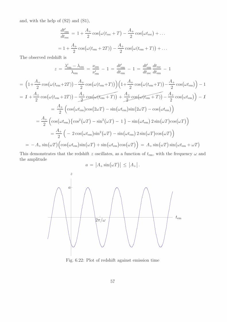
and, with the help of (S2) and (S1),
dt′emdtrec
= 1 +A+
2cos
(
ω(trec + T)
−A+
2cos
(
ωtrec)
+ . . .
= 1 +A+
2cos
(
ω(tem + 2T ))
−A+
2cos
(
ω(tem + T ))
+ . . .
The observed redshift is
z =λ′
em − λem
λem=
νemν ′
em
− 1 =dt′emdtem
− 1 =dt′emdtrec
dtrecdtem
− 1
=(
1+A+
2cos
(
ω(tem+2T ))
−A+
2cos
(
ω(tem+T ))
)(
1+A+
2cos
(
ω(tem+T ))
−A+
2cos
(
ωtem)
)
− 1
= 1 +A+
2cos
(
ω(tem+2T ))
−A+
2cos
(
ω(tem + T ))
+A+
2cos
(
ω(tem + T ))
−A+
2cos
(
ωtem)
)
− 1
=A+
2
(
cos(
ωtem)
cos(
2ωT)
− sin(
ωtem)
sin(
2ωT)
− cos(
ωtem)
)
=A+
2
(
cos(
ωtem)
cos2(
ωT)
− sin2(
ωT)
− 1
− sin(
ωtem)
2 sin(
ωT)
cos(
ωT)
)
=A+
2
(
− 2 cos(
ωtem)
sin2(
ωT)
− sin(
ωtem)
2 sin(
ωT)
cos(
ωT)
)
= −A+ sin(
ωT)
(
cos(
ωtem)
sin(
ωT)
+ sin(
ωtem)
cos(
ωT)
)
= A+ sin(
ωT)
sin(
ωtem + ωT)
This demonstrates that the redshift z oscillates, as a function of tem, with the frequency ω andthe amplitude
a =∣
∣A+ sin(
ωT)∣
∣ ≤∣
∣A+
∣
∣ .
a
tem
z
2π/ω
Fig. 6.22: Plot of redshift against emission time
57

Searches for gravitational waves with the help of Doppler tracking have been carried through,e.g., with Voyager 1 and 2, with Pioneer 10 and 11, and in particular with the Cassini spacecraftthat was launched in 1997 and reached Saturn in 2004. From Fig. 6.23 we can read the frequenciesand the amplitudes of gravitational waves that could have been detected by Doppler trackingof the Cassini spacecraft. We see that this method is sensitive only for low frequencies, around10−3 Hz, and for amplitudes of about 10−16.
Fig. 6.23: from http://www.livingreviews.org/lrr-2006-1
The radio links with spacecraft in the outer region of our Solar system are established with asystem of radio telscopes that is known as the Deep Space Network (DSN). It comprises sites inthe USA, in Spain and in Australia such that at any time of the day at least one of the stationscan communicate with the spacecraft. Fig. 6.24 shows one of the 34-meter telescopes of theDSN, at Goldstone in the Mojave Desert in the USA.
Fig. 6.24: from http://www.livingreviews.org/lrr-2006-1
58

6.4 Pulsar timing arrays
The basic idea of using pulsar timing arrays for detecting gravitational waves is similar to thatof using Doppler tracking. Again, the change of the distance betwen two test masses is measuredwith the help of its effect onto the frequency of a radio signal. In the case of Doppler tracking,the two test masses are the Earth and a spacecraft; in the case of pulsar timing observations theyare a (millisecond) pulsar and the Earth. A major difference is in the fact that pulsar timing isa one-way method (there are signals from the pulsar to the Earth, but no return signals) whileDoppler tracking of spacecraft is a two-way method.
A pulsar emits radio pulses at a rate that is highly stable. For millisecond pulsars, the stabilityof the pulse frequency is comparable to the stablity of the best clocks we have. This, howeverdoes not mean that the pulses arrive with a constant frequency here on Earth. Changes inthe times of arrival are caused e.g. by the relative motion of the pulsar and the Earth, by theinfluence of the gravitatonal field of the Sun and of other masses the signal might pass, and by theinterstellar medium. All these known influences are taken into account in the socalled timingformulas used by radio astronomers for evaluating their observations. Remaining differencesbetween theory and observation are known as timing residuals. A gravitational wave shouldproduce such residuals.
The idea of searching for signatures from gravitational waves in the timing residuals of pulsarswas brought forward by M. Sazhin [“Opportunities for detecting ultralong gravitational waves”Astron. Zh. 55, 65 (1978)] and further developed by S. Detweiler [“Pulsar timing measurementsand the search for gravitational waves” Astrophys. J. 234, 1100 (1979)]. For a recent review onthe planned International Pulsar Timing Array see G. Hobbs et al. [“The International PulsarTiming Array project: using pulsars as a gravitational wave detector” Class. Quantum Grav.27, 084013 (2010)].
Here we will give a calculation under highly idealised assumptions, just to outline the basic idea.We treat the pulsar and the Earth as at rest in a Minkowski background, and we ignore theinfluence of the interstellar medium. The gravitational wave is considered as a perturbation ofthe Minkowski background within the linearised theory,
gµν(x) = ηµν + hµν(x) ,
where the perturbation is assumed to satisfy the following two properties: (i) components witha time index vanish, h0µ = 0, and (ii) the worldlines of constant spatial coordinates, i.e. thecurves
(
xµ(t))
= (ct, ~r0) with a constant ~r0, are geodesics. These two assumptions are satisfied,in particular, if hµν is an arbitrary superposition of gravitational waves in the TT gauge.
By assumption, the worldlines of the pulsar and of the Earth are both t lines. From the form ofthe metric,
gµν(x)dxµdxν = −c2dt2 + δijdx
idxj + hij(x)xidxj ,
we read that along these worldlines the time coordinate t coincides with proper time. Therefore,we can identify frequencies with respect to the time coordinate t with frequencies with respectto proper time of the pulsar or of the Earth. We assume that the pulsar emits signals at a fixedfrequency νP . They will arrive at the Earth with a frequency νE(tE) that depends on the timeof arrival, tE . It is our goal to determine this function νE(tE).
59

~rP
~rE
Earth
pulsar
ni
0Fig. 6.25: Position of the pulsar and of the Earth
Along a light ray from the pulsar to the Earth, we must have
0 = −c2dt2 + δijdxidxj + hij(x)dx
idxj
and thus
c2(
dt
dℓ
)2
= 1 + hij(x)dxi
dℓ
dxj
dℓ
where ℓ denotes arclength with respect to the flat background metric, i.e.
dℓ2 = δijdxidxj .
Without a gravitational wave, the light ray moves on a straight line from the pulsar to the Earth,i.e., dxi/dℓ is a constant unit vecor ni. With a gravitational wave, we have
dxi
dℓ= ni + O(h)
and thus
cdt
dℓ=
√
1 + hij(x)ninj +O(h2) ,
dℓ = c(
1 + hij(x)ninj +O(h2)
)
−1/2
dt = c(
1−1
2hij(x)n
inj + . . .)
dt
where the ellipses indicate terms of quadratic and higher order that will be neglected in thefollowing. Integration over the path of the light ray, from its emission time tP to the arrival timetE , yields
∫ tE
tP
(
1−1
2hij(x)n
inj)
dt =L
c
where L is the distance from the pulsar to the Earth measured in the flat background. Thisequation gives tE as a function of tP . Differentiation with respect to tP yields
dtEdtP
(
1−1
2hij(ctE , ~rE)n
inj)
−
(
1−1
2hkℓ(ctP , ~rP )n
knℓ)
= 0 , ,
dtPdtE
=
(
1−1
2hkℓ(ctE , ~rE)n
knℓ)
(
1−1
2hij(ctP , ~rP )ninj
)
= 1−1
2hkℓ(ctE , ~rE)n
knℓ +1
2hij(ctP , ~rP )n
inj + . . . ,
60

dtPdtE
= 1 +ninj
2
(
hij(ctP , ~rP ) − hij(ctE , ~rE))
.
We have thus found that the pulses, which are emitted with a constant frequency νP , arrive witha frequency νE(tE) given by
νE(tE)− νPνP
=dtPdtE
− 1 =ninj
2
(
hij(ctP , ~rP ) − hij(ctE , ~rE))
.
We see that the frequency shift depends on the projection onto ni of the wave amplitude hij atthe pulsar and at the Earth. If there is a single wave in TT gauge propagating in the x3 direction,ni must have a non-vanishing component in the x1
−x2 plane to give a non-zero frequency shift.If the same gravitational wave is observed with at least three pulsars, the propagation directionof the wave can be deduced.
Pulsar timing arrays are used for many applications; the search for gravitational waves is onlyone of them. Three pulsar timing arrays have been established which routinely observe the timesof arrivals of many pulsars:
• Parkes Pulsar Timing Array (PPTA): This uses the Parkes Telescope in Australia andtakes data since 2005.
• European Pulsar Timing Array (EPTA): This uses data from five radio telescopes in Eu-rope, namely Effelsberg, Jodrell Bank, Westerbork, Nancay, and a new one in Sardinia.
• North American Nanohertz Observatory for Gravitational Waves (NanoGRAV): This is anAmerical pulsar timing array using data from Arecibo and Green Bank.
It is planned to join them into an International Pulsar Timing Array (IPTA), see Hobbs et al.,loc. cit. Great progress with pulsar timing data is expected from the Square Kilometer Array(SKA), an array of radio telescopes in the Southern hemisphere with an effective aperture of asquare kilometer that is planned to be operational around 2020.
Fig. 6.26: from G. Hobbs et al., loc. cit.
Pulsar timing arrays are sensitive to gravitational waves at very low frequencies, between 10−6
and 10−9 Hz, with an amplitude of about 10−15, see Fig. 6.26. Possible sources that could bedetected with this method are merging supermassive black holes.
61

6.5 Influence of gravitational waves on electromagnetic waves
All the methods we have discussed so far were based on measuring the effect of a gravitationalwave onto massive bodies, either onto vibrating masses or onto free test masses. Electromagneticwaves were used in some of these methods, but only as a tool for measuring the effect onto themassive bodies.
In this section we briefly discuss the possibility of detecting a gravitational wave by its effect ontoan electromagnetic wave. One such method was suggested by M. Cruise [“An interaction betweengravitational and electromagnetic waves” Mon. Not. Roy. Astron. Soc. 204, 485 (1983)]. It isbased on the observation that a gravitational wave causes a rotation of the polarisation plane ofan electromagnetic field.
In an arbitrary general-relativistic spacetime, the polarisation vector Π of a linearly polarisedelectromagnetic wave in vacuo is parallely transported along each ray. This can be deduced fromMaxwell’s equations in the high-frequency limit (i.e., in the geometric optics approximation). Ifwe denote the tangent vector to the ray by K, the polarisation vector satisfies the equation
∇KΠ = 0
or, in coordinate notation,Kµ∂µΠ
ρ + ΓρντK
νΠτ = 0 .
The vectors K and Π span the polarisation plane. This plane always contains the directiontangent to the ray, so the only thing it can do is to rotate about this direction. We see that,with respect to the coordinate system used, such a rotation is caused by the Christoffel symbols.For a gravitational wave in TT gauge, we already know that the Christoffel symbols read
Γρντ =
1
2ηρσ Re
(
kνAστ + kτAσν − kσAντ
)
i eikµxµ
where kµ is the wave covector of the gravitational wave. According to this equation, a gravita-tional wave would cause a rotation of the polarisation plane of an electromagnetic wave.
Fig. 6.27: from http://www.sr.bham.ac.uk/gravity
62

The expected rotation angle is tiny. Therefore, Cruise designed a gravitational wave detectorthat would enhance this rotation by making use of a resonance effect. The electromagnetic waveis a radio wave in a wave-guide that is bent into a loop. The resonance frequency of the systemis 100 MHz. If a gravitational wave with the same frequency comes in, the polarisation planeis periodically kicked by a tiny rotation angle in such a way that these tiny rotations add up.Cruise built two such instruments in Birmingham so that he could look for coincidences, seeFig. 6.27. Note that these detectors would be sensitive at a frequency of about 100 MHz, i.e.,at an extremely high frequency in comparison to all other gravitational wave detectors.
In addition to the possibility of constructing non-orthodox gravitational wave detectors, theeffect of a gravitational wave onto electromagnetic waves is of crucial relevance in view of thecosmic background radiation. In recent years several experiments are analysing the polarisationof the cosmic background radiation. In analogy to decomposing a vector field into rotation-free and divergence-free parts, the Fourier components of the cosmic background radiation aredecomposed into electric (E) and magnetic (B) modes. Primordial gravitational waves that havecome into existence through quantum fluctuations in the very early universe would produce aspecific signature of B modes. These B modes from primordial gravitational waves could havea measurable amplitude only if our universe underwent an inflationary period, i.e., a period inwhich the universe expanded exponentially.
In March 2014 it was announced that the BICEP2 experiment had found B modes from pri-mordial gravitational waves in the cosmic background radiation. BICEP2 was a radio telescopenear the South Pole that was operational from 2010 to 2012. If confirmed, the BICEP2 resultwould give strong support for the idea that quantum fluctuations in the early universe haveproduced gravitational waves and that there was an inflationary period. (The idea of primordialgravitational waves, resulting from quantum fluctuations, was developed already in the 1970sby L. Grishchuk and others. The idea of an inflationary universe, brought forward by A. Guth,F. Englert, A. Linde and others around 1980, allowed for an increase in the amplitudes of theseprimordial gravitational waves that could make them measurable.)
Fig. 6.28 summarises the different types of gravitational wave detectors, the frequency range inwhich they are sensitive and the types of sources they could detect.
Fig. 6.28: from http://www.astro.gla.ac.uk
63

7.Gravitationalwaves in the linearised theory around curved spacetime
Up to now we have treated gravitational waves as small perturbations of Minkowski spacetime.We will now modify this approach by allowing for a curved background, still assuming thatthe gravitatonal wave is a small perturbation. Possible applications include the propagation ofgravitational waves with a small amplitude near a black hole.
7.1 Linearised field equation around curved spacetime
We consider a metric of the formgµν =
Bgµν + hµν
whereBgµν is an arbitray Lorentzian (background) metric and the perturbation is assumed to be
so small that all terms of second or higher order with respect to hµν or its derivatives can beneglected. We want to work out the field equation (without a cosmological constant),
Rµν −R
2gµν = κTµν ,
in this linearised theory. As a first step, we have to calculate the Christoffel symbols.
For this chapter, we agree to raise and to lower indices with the background metric. Then, towithin our linear approximation, the inverse metric is of the form
gνρ =Bgνρ
− hνρ .
Proof: gµν(Bgνρ − hνρ
)
=(Bgµν + hµν
)(Bgνρ − hνρ
)
= δρµ + hµρ− hµ
ρ = δρµ.
LetB
Γρµν denote the Christoffel symbols of the background metric and let
B
∇ be the covariantderivative with respect to the background metric. Then the Christoffel symbols of the perturbedspacetime are
Γρµν =
1
2gρσ
(
∂µgσν + ∂νgσµ − ∂σgµν)
=1
2
(Bgρσ
− hρσ)
(
∂µ(Bgσν + hσν
)
+ ∂ν(Bgσµ + hσµ
)
− ∂σ(Bgµν + hµν
)
)
=1
2
Bgρσ
(
∂µBgσν + ∂ν
Bgσµ − ∂σ
Bgµν
)
+1
2
Bgρσ
(
∂µhσν + ∂νhσµ − ∂σhµν
)
−1
2hρσ
(
∂µBgσν + ∂ν
Bgσµ − ∂σ
Bgµν
)
=B
Γρµν +
1
2
Bgρλ
(
∂µhλν + ∂νhλµ − ∂λhµν
)
−1
2
BgρλBgστhλτ
(
∂µBgσν + ∂ν
Bgσµ − ∂σ
Bgµν
)
=B
Γρµν +
1
2
Bgρλ
(
∂µhλν + ∂νhλµ − ∂λhµν − 2B
Γτµνhλτ
)
=B
Γρµν +
1
2
Bgρλ
(B
∇µhλν +B
Γτµλhτν +
B
Γτµνhλτ +
B
∇νhλµ +B
Γτνλhτµ +
B
Γτνµhλτ
−B
∇λhµν −B
Γτλµhτν −
B
Γτλνhµτ −
2B
Γτµνhλτ
)
=B
Γρµν +
1
2
(B
∇µhρν +
B
∇νhρµ −
B
∇ρhµν
)
64

We write this result as
Γρµν =
B
Γρµν + δΓρ
µν
where
δΓρµν =
1
2
(B
∇µhρν +
B
∇νhρµ −
B
∇ρhµν
)
is a tensor field. (Recall that the difference of the Christoffel symbols of two connections is atensor field.)
Next we calculate the curvature tensor.
Rµνρσ = ∂νΓ
µρσ − ∂ρΓ
µνσ + Γµ
νκΓκρσ − Γµ
ρκΓκνσ
= ∂ν
(B
Γµρσ + δΓµ
ρσ
)
− ∂ρ
(B
Γµνσ + δΓµ
νσ
)
+(B
Γµνκ + δΓµ
νκ
)(B
Γκρσ + δΓκ
ρσ
)
−
(B
Γµρκ + δΓµ
ρκ
)(B
Γκνσ + δΓκ
νσ
)
=B
Rµνρσ + ∂νδΓ
µρσ − ∂ρδΓ
µνσ +
B
ΓµνκδΓ
κρσ +
B
ΓκρσδΓ
µνκ −
B
ΓµρκδΓ
κνσ −
B
ΓκνσδΓ
µρκ + . . .
The term indicated by ellipses is of second order and will thus be neglected in the following.This gives us the curvature tensor in the form
Rµνρσ =
B
Rµνρσ + δRµ
νρσ
where
δRµνρσ = ∂νδΓ
µρσ − ∂ρδΓ
µνσ +
B
ΓµνκδΓ
κρσ +
B
ΓκρσδΓ
µνκ −
B
ΓµρκδΓ
κνσ −
B
ΓκνσδΓ
µρκ
=B
∇νδΓµρσ −
B
Γµνκδ
B
Γκρσ +
B
Γκνρδ
B
Γµκσ +
B
Γκνσδ
B
Γµκρ
−B
∇ρδΓµνσ +
B
ΓµρκδΓ
κνσ −
B
ΓκρνδΓ
µκσ −
B
ΓκρσδΓ
µκν
+B
ΓµνκδΓ
κρσ +
B
ΓκρσδΓ
µνκ −
B
ΓµρκδΓ
κνσ −
B
ΓκνσδΓ
µρκ
=B
∇νδΓµρσ −
B
∇ρδΓµνσ .
With our earlier result for δΓµρσ this can be rewritten as
δRµνρσ =
1
2
B
∇ν
(B
∇ρhµσ +
B
∇σhµρ −
B
∇µhρσ
)
−1
2
B
∇ρ
(B
∇νhµσ +
B
∇σhµν −
B
∇µhνσ
)
=1
2
(B
∇ν
B
∇ρhµσ +
B
∇ν
B
∇σhµρ −
B
∇ν
B
∇µhρσ −
B
∇ρ
B
∇νhµσ −
B
∇ρ
B
∇σhµν +
B
∇ρ
B
∇µhνσ
)
.
65

Contraction gives the Ricci tensor
Rνσ =B
Rνσ + δRνσ
where
δRνσ = δRµνµσ =
1
2
(
B
∇ν
B
∇µhµσ +
B
∇ν
B
∇σh−
B
∇ν
B
∇µhµσ −
B
∇µ
B
∇νhµσ −
B
∇µ
B
∇σhµν +
B
hνσ
)
.
Here we have introduced the trace of the perturbation,
h = hµµ =Bgµνhµν ,
and the wave operator of the background metric,
B
=B
∇µ
B
∇µ =
Bgµν
B
∇µ
B
∇ν .
If we contract another time we get the Ricci scalar
R =B
R + δR
with
δR = δRνν =
1
2
(B
∇νB
∇νh−B
∇µ
B
∇νhµν −
B
∇µ
B
∇νhµν +
B
hνν
)
=B
h −B
∇µ
B
∇νhµν .
Finally, the Einstein tensor reads
Gµν =B
Gµν + δGµν
where
δGµν = δ(
Rµν −1
2Rgµν
)
= δRµν −1
2R δgµν −
1
2δR gµν = δRµν −
1
2
B
Rhµν −1
2δR
Bgµν + . . .
=1
2
(B
hµν +B
∇µ
B
∇νh−B
∇ρ
B
∇µhνρ−
B
∇ρ
B
∇νhµρ−
B
Rhµν −Bgµν
(B
h−B
∇ρ
B
∇σhρσ))
.
Now we use that the commutator of covariant derivatives can be expressed in terms of thecurvature tensor,
(B
∇ρ
B
∇µ −B
∇µ
B
∇ρ
)hν
ρ =B
Rτρµνhτ
ρ−
B
Rρρµτhν
τ .
We find
B
∇ρ
B
∇µhνρ +
B
∇ρ
B
∇νhµρ =
B
∇µ
B
∇ρhνρ−
B
Rτµρνhτ
ρ +B
Rρµρτhν
τ +B
∇ν
B
∇ρhµρ−
B
Rτνρµhτ
ρ +B
Rρνρτhµ
τ .
This can be rewritten, with the curvature identities
B
Rτµντ +
B
Rτντµ +
B
Rττµν = 0 ,
B
Rτµρν = −
B
Rτρµν ,
66

as
B
∇ρ
B
∇µhνρ+
B
∇ρ
B
∇νhµρ =
B
∇µ
B
∇ρhνρ+
B
Rτρµνhτ
ρ+B
Rµτhντ+
B
∇ν
B
∇ρhµρ+
(B
Rτρµν+
B
Rτµνρ
)hτ
ρ+B
Rντhµτ
=B
∇µ
B
∇ρhνρ + 2
B
Rτρµνhτ
ρ +B
Rµτhντ +
B
∇ν
B
∇ρhµρ +
B
Rτµνρhτρ
︸ ︷︷ ︸
=0
+B
Rντhµτ
where the underbraced term vanishes because of the curvature identityB
Rτµνρ = −B
Rρµντ . Insert-ing this expression into our result for δGµν gives
2 δGµν =B
hµν +B
∇µ
B
∇νh−B
∇µ
B
∇ρhνρ− 2
B
Rτρµνhτ
ρ−
B
Rµτhντ
−B
∇ν
B
∇ρhµρ−
B
Rντhµτ−
B
Rhµν −Bgµν
(B
h−B
∇ρ
B
∇σhρσ)
.
This is the general expression for δGµν on an arbitrary background spacetime. From now on wespecify to the case that the background spacetime satisfies the vacuum field equation (withouta cosmological constant),
B
Rµν = 0 .
Then
2 δGµν =B
hµν +B
∇µ
B
∇νh−B
∇µ
B
∇ρhνρ− 2
B
Rτρµνhτ
ρ−
B
∇ν
B
∇ρhµρ−
Bgµν
(B
h−B
∇ρ
B
∇σhρσ)
.
This expression can be simplified if we use the gauge freedom. We follow our treatment in thecase of a flat background (see p.8/9) as closely as possible. We introduce
γµν = hµν −h
2
Bgµν
which implies
γ :=Bgµνγµν = h −
1
24 h = −h ,
hencehµν = γµν −
γ
2
Bgµν .
Then our expression for δGµν reads
2 δGµν =B
(
γµν −γ
2
Bgµν
)
−B
∇µ
B
∇νγ −B
∇µ
B
∇ρ
(
γνρ−γ
2δρν
)
−2B
Rτρµν
(
γτρ−γ
2δρτ
)
−B
∇ν
B
∇ρ
(
γµρ−γ
2δρµ
)
+Bgµν
B
γ +Bgµν
B
∇ρ
B
∇σ
(
γρσ −γ
2
Bgρσ
)
=B
γµν −1
2
Bgµν
B
γ −B
∇µ
B
∇νγ −B
∇µ
B
∇ργνρ +
1
2
B
∇µ
B
∇νγ − 2B
Rτρµνγτ
ρ +B
Rρρµν
︸ ︷︷ ︸
=0
γ
67

−B
∇ν
B
∇ργµρ +
1
2
B
∇ν
B
∇µγ +
Bgµν
B
γ +Bgµν
B
∇ρ
B
∇σγρσ
−
1
2
Bgµν
B
γ
=B
γµν −B
∇µ
B
∇ργνρ− 2
B
Rτρµνγτ
ρ−
B
∇ν
B
∇ργµρ +
Bgµν
B
∇ρ
B
∇σγρσ
We can now make a coordinate transformation of the form
xµ 7→ xµ + fµ(x)
where fµ(x) is small of first order, i.e., so small that only terms linear in fµ and its derivativeshave to be kept. Then the metric transforms as
gµν(x)dxµdxν 7→ gµν
(x+ f
)(dxµ + ∂ρf
µ(x)dxρ)(dxν + ∂σf
ν(x)dxσ)
= gµν(x)dxµdxν + ∂σgµν(x)f
σ(x)dxµdxν + ∂ρfµ(x)gµν(x)dx
ρdxν + ∂σfν(x)gµν(x)dx
µdxσ + . . .
=(
gµν(x) + ∂σgµν(x)fσ(x) + ∂µf
ρ(x)gρν(x) + ∂νfσ(x)gµσ(x)
)
dxµdxν
i.e.Bgµν + hµν 7→
Bgµν + hµν + fσ∂σ
Bgµν +
Bgρν∂µf
ρ +Bgµσ∂νf
σ + . . .
hencehµν 7→ hµν + fσ∂σ
Bgµν +
Bgρν∂µf
ρ +Bgµσ∂νf
σ + . . .
= hµν + f τ∂τBgµν +
Bgρν
(B
∇µfρ−
B
Γρµτf
τ)+
Bgµσ
(B
∇νfσ−
B
Γσντf
τ)
= hµν+B
∇µfν+B
∇νfµ+fτ(
∂τBgµν−
1
2
Bgρν
Bgρσ
(∂µ
Bgστ+∂τ
Bgσµ−∂σ
Bgµτ
)−1
2
Bgµσ
Bgσρ
(∂ν
Bgρτ+∂τ
Bgρν−∂ρ
Bgντ
))
= hµν +B
∇µfν +B
∇νfµ + f τ(
∂τBgµν −
1
2
(
∂µBgντ +
∂τBgνµ −
∂νBgµτ
)−
1
2
(
∂νBgµτ +
∂τBgµν −
∂µBgντ
))
= hµν +B
∇µfν +B
∇νfµ .
This implies
h 7→ h+ 2B
∇σfσ
or equivalently
γ 7→ γ − 2B
∇σfσ ,
and
γµν = hµν −h
2
Bgµν 7→ hµν +
B
∇µfν +B
∇νfµ −1
2
(h+2
B
∇σfσ)Bgµν = γµν +
B
∇µfν +B
∇νfµ −B
∇σfσBgµν .
68

Hence, the covariant divergence of γµν transforms according to
B
∇µγµν 7→
B
∇µγµν +
B
∇µB
∇µfν +B
∇µB
∇νfµ −B
∇µB
∇σfσBgµν
=B
∇µγµν +
B
fν +B
∇σ
B
∇νfσ−
B
∇ν
B
∇σfσ =
B
∇µγµν +
B
fν +B
Rσσντ
︸ ︷︷ ︸
=0
f τ .
If fµ is chosen such that
B
fν = −B
∇µγµν , (WE)
the covariant divergence of γµν is transformed to zero. (In general, a solution fµ to the inho-mogeneous wave equation (WE) does not exist globally on the spacetime manifold, unless thespacetime is what is called “globally hyperbolic”. However, it does exist on a certain neighbour-hood of a spacelike hypersurface, by giving initial data on this spacelike hypersurface. In thefollowing we are satisfied with having coordinates with the desired property on such a neigh-bourhood.) Then
2 δGµν =B
γµν − 2B
Rτρµνγτ
ρ .
We still have the freedom of making coordinate transformations xµ 7→ xµ+fµ(x) withB
fµ = 0.Up to now we have assumed that the background metric satisfies the vacuum field equation.From now on we will assume, in addition, that the perturbed spacetime satisfies the vacuumfield equation as well. Then we get
B
γµν − 2B
Rτρµνγτ
ρ = 0 . (∗)
In this case we can use the remaining gauge freedom to make the trace γ = −h to zero, so thatγµν = hµν .
Proof: We can still make transformations xµ 7→ xµ + fµ(x) withB
fµ = 0. Thiswave equation has a unique solution if initial data fµ(x0 = 0) and ∂0f
µ(x0 = 0) areprescribed. Here we assume that x0 = 0 is a spacelike hypersurface; then the solutionis defined on a neighbourhood of this hypersurface. We have to show that we can
choose the initial data such that the solution fµ satisfies 2B
∇µfµ− γ = 0. We first
observe that the expression ψ = 2B
∇µfµ− γ satisfies the wave equation:
B
ψ = 2B
∇νB
∇ν
B
∇µfµ−
B
γ = 2B
∇ν(B
∇µ
B
∇νfµ +
B
Rµνµσ
︸ ︷︷ ︸
=0
fσ)−
B
γ = 2B
∇ν
B
∇µ
B
∇νfµ
−B
γ
= 2(B
∇µ
B
∇ν
B
∇νfµ
− Rννµσ
︸ ︷︷ ︸
=0
B
∇σfµ
−Rµνµσ
︸ ︷︷ ︸
=0
B
∇νfσ
)−
B
γ = 2B
∇µ
B
fµ
︸︷︷︸
=0
−B
γ = 0
where the last equality follows from taking the trace of (∗). This demonstrates thatψ is uniquely determined by its initial data ψ(x0 = 0) and ∂0ψ(x
0 = 0). If we can
69

choose the initial data for fµ such that ψ(x0 = 0) = 0 and ∂0ψ(x0 = 0) = 0, then ψ
must vanish everywhere. As
ψ = 2B
∇µfµ− γ = 2
B
∇0f0 + 2
B
∇ifi− γ
does not involve x0 derivatives of the f i, and
∂0ψ =B
∇0ψ = 2Bg00
B
∇0B
∇0f0 + 2
B
∇0
B
∇ifi−
B
∇0γ = −2Bg00
B
∇iB
∇if0 + 2
B
∇0
B
∇ifi−
B
∇0γ
does not involve an x0 derivative of f 0, such a choice of initial data is indeed possible.
As the main result of this section, we have found that the linearised vacuum field equation reads
B
hµν − 2B
Rτρµνhτ
ρ = 0
in a gauge such thatB
∇µhµν = 0 , h = 0 .
We have shown that such a gauge is possible. Obviously, our gauge generalises the Hilbert gaugeto the case of a curved background and it incorporates, in addition, the consition that the tracevanishes. Note, however, that it does not reproduce emphall properties of the TT gauge thatwe have discussed for plane-harmonic waves on flat background. In contrast to the TT gauge, isnot in general possible to choose the coordinates on our curved background such that h0µ = 0.
We see that, even in the most convenient gauge, the linearised vacuum field equation on acurved background is not just the ordinary wave equation for hµν but it contains an additionalcurvature term. This term somewhat resembles the mass term in the Klein-Gordon equation,B
ψ −m2ψ = 0.
7.2 “Geometric optics” of gravitational waves on a curved background
We will now discuss how gravitational waves propagate, on a curved background, in the high-frequency limit. This is the gravitational-wave analogue of geometric optics. In the last section
we have seen that, in a gauge withB
∇µhµν = 0 and h = 0, the linearised vacuum field equation
readsB
hµν − 2B
Rτρµνhτ
ρ = 0 .
On a flat background, we have found plane-wave solutions which are of the form
hµν(x) = ReAµνe
kσxσ
with a constant complex amplitude Aµν and a constant real wave covector kµ. In the case of acurved background, exact solutions of this form do not exist. However, we can start out withthe more general ansatz
hµν(x) = Reh(0)µν (x)e
iφ(x)
70

where h(0)µν (x) is a complex-valued function of x and φ(x) is a real-valued function of x. With this
ansatz we want to find approximate solutions that resemble plane-harmonic waves in sufficientlysmall spacetime regions. In the following we drop the “Re” sign to ease notation, but it is alwaysunderstood that the real part is to be taken.
With our ansatz, we calculate
B
hµν =B
∇σB
∇σ
(h(0)µν e
iφ)=
B
∇σ(
eiφ(B
∇σh(0)µν + h(0)µν i
B
∇σφ))
= eiφ(B
∇σB
∇σh(0)µν +
B
∇σh(0)µν i
B
∇σφ+
B
∇σh(0)µν i
B
∇σφ+ h(0)µν iB
∇σB
∇σφ+ h(0)µν iB
∇σφi
B
∇σφ)
= eiφ(B
h(0)µν − h(0)µν
B
∇σφ
B
∇σφ+ i(2B
∇σh(0)µν
B
∇σφ+ h(0)µν
B
φ))
.
Feeding this expression into the linearised field equation yields
eiφ(B
h(0)µν − h(0)µν
B
∇σφ
B
∇σφ+ i(2B
∇σh(0)µν
B
∇σφ+ h(0)µν
B
φ))
− 2B
Rτρµνh
(0)τ
ρeiφ = 0 ,
h(0)µν
B
∇σφ
B
∇σφ+ i(2B
∇σh(0)µν
B
∇σφ+ h(0)µν
B
φ)+ h(0)µν
B
φ)+
B
h(0)µν − 2B
Rτρµνh
(0)τ
ρ = 0 .
We now impose the approximations that allow to interpret our hµν(x) as an approximate plane-harmonic wave. To that end we assume that the phase varies more rapidly than the amplitude.We fix an event with coordinates x0 and we consider a neighbourhood of x0 that is so small thatthe amplitude can be treated as almost constant on this neighbourhood but φ varies such thatit can be written, approximately, as
φ(x) ≈ φ(x0) +B
∇µφ(x0)(xµ − x
µ0
).
As the constant phase factor ei(φ(x0)−
B
∇µφ(x0)xµ0
)
can be absorbed into the amplitude, this meansthat our hµν can be approximated as a plane-harmonic wave with wave covector
kµ =B
∇µφ(x0) .
As this can be done around any point, the functionB
∇µφ can be interpreted as the covector fieldof our approximate plane-harmonic wave. If we split this into temporal and spatial parts, we
may say thatB
∇0φ gives the frequency (up to a factor of c) and that theB
∇iφ give the componentsof the spatial wave covector.
If we adopt this approximation scheme, terms which are quadratic in the derivatives of φ arebigger than terms that are linear in the derivatives of φ, and the latter are bigger than termswhich do not involve any derivatives of φ. This can be done, in a more formal way, by writinga book-keeping parameter α in front of the phase and then comparing equal orders of α. Thehighest-order term in the linearised field equation is a second-order term in α. Equating it tothe zero on the right-hand side yields
h(0)µν
B
∇σφ
B
∇σφ = 0, . (F0)
71

Next we get two first-order terms which require
2B
∇σh(0)µν
B
∇σφ+ h(0)µν
B
φ = 0 . (F1)
Finally, the zeroth-order terms give
B
h(0)µν − 2B
Rτρµνh
(0)τ
ρ = 0 . (F2)
As the amplitude has, of course, to be non-zero almost everywhere to give a non-trivial wave,
(F0) says that the wave covector field kµ =B
∇µφ is lightlike,
Bgµνkµkν = 0 .
This implies that the integral curves of the wave vector field kν =Bgνµkµ =
Bgνµ
B
∇µφ are lightlikegeodesics.
Proof: Obviously,Bgµνk
µkν =Bgµνkµkν = 0 ,
so the integral curves of kν are lightlike. What we still have to show is that they aregeodesics, i.e., that
kµB
∇µkρ = 0 .
To that end, we apply the covariant derivative operator to the equation
0 =Bgµνkµkν
which results in
0 =B
∇ρ
(Bgµνkµkν
)= 2
Bgµν
(B
∇ρkµ)kν = 2kµ
(B
∇ρ
B
∇µφ)= 2kµ
B
∇µ
B
∇ρφ = 2kµB
∇µkρ
where we have used that, for a scalar field φ,
B
∇µφ = ∂µφ ,
hence
B
∇ρ
B
∇µφ =B
∇ρ∂µφ = ∂ρ∂µφ− Γσρµ
B
∇σφ = ∂µ∂ρφ− Γσµρ
B
∇σφ =B
∇µ∂ρφ =B
∇µ
B
∇ρφ .
We have thus shown that, to within the linearised theory on a curved background, the rays ofgravitational waves behave precisely as the rays of electromagnetic waves, i.e., that “gravitationalwaves propagate at the speed of light”.
Now we evaluate the remaining equations (F1) and (F2). To that end we introduce the nor-malised amplitude
h(0)µν (x) =h(0)µν (x)
H(x), H(x) :=
√
h(0)ρτ (x)h(0)ρτ (x) .
72

From (F1), which can be rewritten as
2kσB
∇σh(0)µν = −h(0)µν
B
∇λ
B
∇λφ = −h(0)µν
B
∇λkλ ,
we find
kσB
∇σH = kσB
∇σ
√
h(0)µν h(0)µν =
2h(0)µνkσB
∇σh(0)µν
2
√
h(0)ρτ h(0)ρτ
=−h(0)µνh
(0)µν
B
∇λkλ
2H=
−H2B
∇λkλ
2H=
−H
2
B
∇λkλ .
With this information, we evaluate (F1) in the following way.
0 = 2kσB
∇σh(0)µν + h(0)µν
B
∇λkλ = 2kσ
B
∇σ
(Hh(0)µν
)+ h(0)µν
B
∇λkλ
= 2kσ(H
B
∇σh(0)µν + h(0)µν
B
∇σH)+ h(0)µν
B
∇λkλ = 2kσH
B
∇σh(0)µν +
2h(0)µν
(−H
2
B
∇λkλ)
+
h(0)µν
B
∇λkλ .
As H is non-zero almost everywhere, the last equation implies
kσB
∇σh(0)µν = 0 ,
i.e., the normalised amplitude tensor is parallely transported along each ray. This result isagain completely analogous to the electrodynamic case, where the polarisation vector is parallelytransported along each ray.
Finally, we have to take (F2) into account. This equation implies that, on a non-flat background,
the amplitude h(0)µν is not in general constant.
We emphasise that our approximation scheme was based on the idea of comparing equal powersof derivatives of φ. By adopting this approximation scheme, we have not only assumed that theamplitude is varying slowly in comparison to the phase; we have also assumed that the curvatureterm in the linearised field equation is small in comparison to the square of the derivative of φ.By contrast, if the curvature term is of the same order as the square of the derivative of φ, itmoves from (F2) to (F0), i.e., (F0) has to be replaced with
Bgσρ
B
∇σφ
B
∇σφ− 2B
Rτρµνh
(0)τ
ρ = 0 .
In this case, it is not true that that the rays of gravitational waves are lightlike geodesics;the background curvature produces a modification of the dispersion relation, i.e., of the relationbetween frequency and wavelength of a gravitational wave. The question of which approximationis justified depends on the physical situation: If the curvature of the spacetime is small incomparison to λ−2, our original approximation is valid; if it is of the same order of magnitude,the latter approximation is valid. Here λ denotes the wavelength of the gravitational wave.(Note that the curvature tensor has dimension length−2.)
73

7.3 Linearised field equation on Schwarzschild spacetime
In Section 7.1 we have derived the linearised vacuum field equation on a curved background inthe form
B
hµν − 2B
Rτρµνhτ
ρ = 0
which is valid only in a gauge such thatB
∇µhµν = 0 and h = 0 . As an alternative, we can writethe linearised vacuum field equation in the form
0 = δRνσ = δRµνµσ =
B
∇νδΓµµσ −
B
∇µδΓµνσ
which is true in any gauge, see p.65. In the following we will use the latter form because it leavesus the freedom of making arbitrary gauge transformations.
It is our goal to evaluate this equation for the case that the background metric is the Schwarzschildspacetime,
Bgµνdx
µdxν = −(
1− rS
r
)
c2dt2 +dr2
(
1− rS
r
) + r2(dϑ2 + sin2ϑ dϕ2
).
For later purpose, we list the non-vanishing Christoffel symbols of the Schwarzschild spacetime:
B
Γtrt =
B
Γttr =
rS
2r2(
1− rS
r
) ,
B
Γrrr =
− rS
2r2(
1− rS
r
) ,B
Γrtt =
c2rS
2r2
(
1− rS
r
)
,B
Γrϕϕ = −r
(
1− rS
r
)
sin2ϑ ,B
Γrϑϑ = − r
(
1− rS
r
)
B
Γϑrϑ =
B
Γϑϑr =
1
r,
B
Γϑϕϕ = − sin ϑ cosϑ
B
Γϕϑϕ =
B
Γϕϕϑ = cotϑ ,
B
Γϕrϕ =
B
Γϕϕr =
1
r
As the Schwarzschild spacetime is static and spherically symmetric, we can separate off the timepart and the angle part so that, in the end, we are left with an ordinary differential equationfor the radial part. The procedure is quite analogous to solving the Schrodinger equation with atime-independent spherically symmetric potential: One splits off the time part
(∼ e
iωt)and the
angle part(∼ Yℓm(ϑ, ϕ)
)and is then left with an ordinary differential equation for the radial
part; in the case of the Coulomb potential, this radial differential equation has the Laguerrepolynomials as the solutions.
In the case at hand, the situation is considerably more complicated than in the case of theSchrodinger equation as our unknown function is not a scalar ψ but a tensor field hµν . Therefore,we have to deal with vectorial and tensorial spherical harmonics in addition to the ordinary(scalar) spherical harmonics Yℓm(ϑ, ϕ). Also, the gauge freedom has to be taken into account.Instead of beginning with splitting off the time part, as one usual does with the Schrodingerequation, it is more convenient to do this at the very end. We proceed in the following five steps.
74
Step 1: Expand hµν(t, r, ϑ, ϕ) in terms of spherical harmonics.
Step 2: Decompose hµν(t, r, ϑ, ϕ) into parts that are even and odd, respectively, with respectto parity transformations.
Step 3: Restrict to the odd parts. Simplify hµν(t, r, ϑ, ϕ) with the help of an appropriate gaugetransformation.
Step 4: Insert this simplified expression into the linearised vacuum field equation. After anappropriate substitution this results in one equation for one scalar function Qℓm(t, r),known as the time-dependent Regge-Wheeler equation [T. Regge, J. Wheeler: “Stabilityof a Schwarzschild singularity” Phys. Rev. 108, 1063 (1957)].
Step 5: Separate off the time part to get an ordinary differential equation for a funcion thatdepends on the radial variable only, known as the time-independent Regge-Wheeler equa-tion.
The treatment of perturbations that are even with respect to parity transformations is consid-erably more difficult. We will not work this out here. In the end, also in this case one arrives ata Regge-Wheeler type equation for a radial function with an effective potential. It is called theZerilli equation and was found only 13 years after the Regge-Wheeler paper [F. Zerilli: “Effec-tive potential for even-parity Regge-Wheeler gravitational perturbation equations”, Phys. Rev.Lett. 24, 737 (1970)].
Step 1: As a preparation for expanding the metric perturbation into spherical harmonics, wewrite it in the form
hµν(t, r, ϑ, ϕ)dxµdxν = hAB(t, r, ϑ, ϕ)dx
AdxB
+2 hAΣ(t, r, ϑ, ϕ)dxAdxΣ + hΣΩ(t, r, ϑ, ϕ)dx
ΣdxΩ .
Here and in the following, indices A,B,C, . . . take values r and t while indices Σ,Ω,∆, . . .take values ϑ and ϕ. Recall that two covector fields without a symbol between them meansthe symmetrised tensor product, dxAdxΣ = 1
2
(dxA ⊗ dxΣ + dxΣ ⊗ dxA
). We see that, with
respect to the angular part, the perturbation splits into three scalar functions hAB, twocovector fields hAΣdx
Σ and a symmetric second-rank tensor field hΣΩdxΣdxΩ. We do the
expansion into spherical harmonics for these three cases separately.
Scalar part: For fixed (t, r), we have three scalar functions htt, hrt = htr and hrr on thesphere. These can be expanded into the usual (scalar-valued) spherical harmonics. Fornon-negative m, they are defined as
Yℓm(ϑ, ϕ) = CℓmPℓm
(cosϑ
)eimϕ
where the Pℓm are the associated Legendre polynomials,
Pℓm(x) = (−1)m(1− x2)m/2( d
dx
)m
Pℓ(x) ,
the Pℓ are the Legendre polynomials,
Pℓ(x) =1
2ℓℓ!
( d
dx
)ℓ
Pℓ
(x2 − 1
)ℓ,
75

and the Cℓm are normalisation factors,
Cℓm =
√
(2ℓ+ 1)(l −m)!
4π(ℓ+m)!.
The definition is extended to the case of negative m by requiring
Yℓ(−m)(ϑ, ϕ) = (−1)mYℓm(ϑ, ϕ)
where overlining means complex conjugation. ℓ runs over all integers from 0 to ∞ and mruns, for fixed ℓ, over all integers from −ℓ to ℓ.
Expanding with respect to spherical harmonics gives us the scalar parts of the metricperturbation as
hAB(t, r, ϑ, ϕ) =∞∑
ℓ=0
ℓ∑
m=−ℓ
uABℓm(t, r)Yℓm(ϑ, ϕ) .
Covector part: For fixed (t, r), we have two covector fields htΣdxΣ and hrΣdx
Σ on thesphere. The coefficients hAΣ are scalar-valued functions on the sphere, so one could expandthem in terms of the scalar-valued spherical harmonics Yℓm. However, this would notbe meaningful because the hAΣ are not invariant scalar functions; they change if a newcoordinate basis is chosen on the sphere. To get an expansion that respects the invarianceproperties of the mathematical objects, one needs (co)vector-valued spherical harmonics.As the sphere is two-dimensional, we need two such sets for a basis. There are differentchoices for such a basis. Here we choose the same basis as Regge and Wheeler: For thefirst set we choose the gradients of the Yℓm, which clearly have the correct transformationbehaviour as covector fields,
ΨℓmΣ(ϑ, ϕ)dxΣ =
B
∇ΣYℓm(ϑ, ϕ)dxΣ .
The second set is constructed orthogonal to the first set,
ΦℓmΣ(ϑ, ϕ)dxΣ = εΣΩ
B
∇ΩYℓm(ϑ, ϕ)dxΣ ,
whereεΣΩdx
Σ ⊗ dxΩ = r2sin ϑ(dϑ⊗ dϕ− dϕ⊗ dϑ
)
is the Levi-Civita tensor field (volume form) on the sphere. The latter is defined by theproperties that it is anti-symmetric, εΣΩ = −εΩΣ, and that it evaluates to unity on anorthonormal basis,
(
εΣΩdxΣ ⊗ dxΩ
)( ∂ϑ√
Bgϑϑ
,∂ϕ
√Bgϕϕ
)
=εϑϕ
√Bgϑϑ
Bgϕϕ
=r2sinϑ√r2r2sin2ϑ
= 1 .
As the covariant derivative of a scalar function is the same as the partial derivative, the(co)vector-valued spherical harmonics can be rewritten as
ΨℓmΣ(ϑ, ϕ)dxΣ = ∂ϑYℓm(ϑ, ϕ)dϑ + ∂ϕYℓm(ϑ, ϕ)dϕ ,
76

ΦℓmΣ(ϑ, ϕ)dxΣ = εϑϕ
Bgϕϕ∂ϕYℓm(ϑ, ϕ)dϑ + εϕϑ
Bgϑϑ∂ϑYℓm(ϑ, ϕ)dϕ
= r2sinϑ
1
r2sin2ϑ
∂ϕYℓm(ϑ, ϕ)dϑ − r2sinϑ
1
r2∂ϑYℓm(ϑ, ϕ)dϕ
=1
sinϑ∂ϕYℓm(ϑ, ϕ)dϑ − sin ϑ ∂ϑYℓm(ϑ, ϕ)dϕ .
We expand the covector parts of the metric perturbation with respect to this basis as
hAΣdxΣ =
∞∑
ℓ=0
ℓ∑
m=−ℓ
(
vAℓm(t, r)ΨℓmΣ + vAℓm(t, r)ΦℓmΣ
)
dxΣ .
Tensor part: For fixed (t, r), we have a symmetric second-rank tensor field hΣΩdxΣdxΩ
on the sphere. On a two-dimensional space, a symmetric second-rank tensor has threeindependent components, so we need three sets of tensor-valued spherical harmonics for abasis. Again, we choose the basis in the same way as Regge and Wheeler. As the secondcovariant derivative of a scalar function gives a symmetric second-rank tensor field, wechoose for the first set
ΨℓmΣΩ(ϑ, ϕ)dxΣdxΩ =
(B
∇Σ
B
∇ΩYℓm
)
(ϑ, ϕ)dxΣdxΩ .
As the angular part of the metric,BgΣΩ, is a symmetric second-rank tensor field proportional
to r2, we choose for the second set
ΦℓmΣΩ(ϑ, ϕ)dxΣdxΩ =
(
Yℓm
BgΣΩ
r2
)
(ϑ, ϕ)dxΣdxΩ .
The third set we construct, in analogy to our procedure in the covector case, orthogonalto the ΨℓmΣΩ,
χℓmΣΩ(ϑ, ϕ)dxΣdxΩ =
1
2
(
εΣ∆
B
∇∆B
∇ΩYℓm + εΩ∆
B
∇∆B
∇ΣYℓm
)
(ϑ, ϕ) dxΣ dxΩ .
With the help of the Christoffel symbols listed at the beginning of this section, the tensor-valued spherical harmonics can be rewritten as
ΨℓmΣΩ(ϑ, ϕ)dxΣdxΩ =
B
∇ϑ
B
∇ϑYℓm(ϑ, ϕ)dϑ2 + 2
B
∇ϑ
B
∇ϕYℓm(ϑ, ϕ)dϑdϕ+B
∇ϕ
B
∇ϕYℓm(ϑ, ϕ)dϕ2
= ∂2ϑYℓm(ϑ, ϕ)dϑ2+2
(
∂ϑ∂ϕYℓm−B
Γϕϑϕ∂ϕYℓm
)
(ϑ, ϕ)dϑdϕ+(
∂2ϕYℓm−B
Γϑϕϕ∂ϑYℓm
)
(ϑ, ϕ)dϕ2
= ∂2ϑYℓm(ϑ, ϕ)dϑ2 + 2
(
∂ϑ∂ϕYℓm(ϑ, ϕ)− cotϑ ∂ϕYℓm(ϑ, ϕ))
dϑdϕ
+(
∂2ϕYℓm(ϑ, ϕ) + sin ϑ cosϑ ∂ϑYℓm(ϑ, ϕ))
dϕ2 ,
ΦℓmΣΩ(ϑ, ϕ)dxΣdxΩ = Yℓm(ϑ, ϕ)
(Bgϑϑ
r2dϑ2 +
Bgϕϕ
r2dϕ2
)
= Yℓm(ϑ, ϕ)(dϑ2 + sin2ϑ dϕ2
),
77
χℓmΣΩ(ϑ, ϕ)dxΣdxΩ =
(
εϑϕBgϕϕ
B
∇ϕ
B
∇ϑYℓm
)
(ϑ, ϕ)dϑ2 +(
εϑϕBgϕϕ
B
∇ϕ
B
∇ϕYℓm
)
(ϑ, ϕ)dϑdϕ
+(
εϕϑBgϑϑ
B
∇ϑ
B
∇ϑYℓm
)
(ϑ, ϕ)dϕdϑ+(
εϕϑBgϑϑ
B
∇ϑ
B
∇ϕYℓm
)
(ϑ, ϕ)dϕ2
=r2sinϑ
r2sin2ϑ
(
∂ϕ∂ϑYℓm −B
Γϕϕϑ∂ϕYℓm
)
(ϑ, ϕ)dϑ2 +r2sinϑ
r2sin2ϑ
(
∂2ϕYℓm −B
Γϑϕϕ∂ϑYℓm
)
(ϑ, ϕ)dϑdϕ
−r2sinϑ
r2
∂2ϑYℓm(ϑ, ϕ)dϑdϕ− r2sinϑ
r2
(
∂ϑ∂ϕYℓm(ϑ, ϕ)−B
Γϕϑϕ∂ϕYℓm
)
dϕ2
=1
sinϑ
(
∂ϕ∂ϑYℓm(ϑ, ϕ)− cotϑ ∂ϕYℓm(ϑ, ϕ))(dϑ2 − sin2ϑ dϕ2
)
+1
sinϑ
(
∂2ϕYℓm(ϑ, ϕ)− sin2ϑ ∂2ϑYℓm(ϑ, ϕ) + sinϑ cosϑ ∂ϑYℓm(ϑ, ϕ))
dϑdϕ .
We expand the tensorial part of the metric perturbation in the form
hΣΩ(t, r, ϑ, ϕ)dxΣdxΩ =
∞∑
ℓ=0
ℓ∑
m=−ℓ
(
wℓm(t, r)ΨℓmΣΩ(ϑ, ϕ) + wℓm(t, r)ΦℓmΣΩ(ϑ, ϕ) + wℓm(t, r)χℓmΣΩ(ϑ, ϕ))
dxΣdxΩ .
Step 2: We will now investigate the transformation behaviour of our various spherical harmonicswith respect to parity transformations (i.e., reflections at the origin)
(ϑ, ϕ) 7→ (π − ϑ, ϕ+ π) .
Obviously, under such a transformation
cosϑ 7→ − cosϑ , sinϑ 7→ sinϑ , eimϕ 7→ e
imϕeimπ = e
imϕ(eiπ)m
= eimϕ(−1)m ,
dϑ 7→ − dϑ , dϕ 7→ dϕ , ∂ϑ 7→ − ∂ϑ , ∂ϕ 7→ ∂ϕ ,
We also need to know that
Pℓ(−x) =1
2ℓℓ!
(
− d
dx
)ℓ
Pℓ
(x2 − 1
)ℓ= (−1)ℓPℓ(x) ,
Pℓm(−x) = (−1)m(1− x2)m/2(
− d
dx
)m
Pℓ(−x) = (−1)m(−1)ℓPℓm(x) .
We introduce the following terminology. A function Fℓm(ϑ, ϕ) is said to be
• even under parity transformations if Fℓm(π − ϑ, ϕ + π) = (−1)ℓFℓm(ϑ, ϕ),
• odd under parity transformations if Fℓm(π − ϑ, ϕ + π) = (−1)ℓ+1Fℓm(ϑ, ϕ).
Instead of even/odd, some authors say polar/axial, electric/magnetic or poloidal/toroidal.
With the help of the above transformation rules, we will now demonstrate that
78

Yℓm(ϑ, ϕ) is even,
ΨℓmΣ(ϑ, ϕ)dxΣ is even,
ΦℓmΣ(ϑ, ϕ)dxΣ is odd,
ΨℓmΣΩ(ϑ, ϕ)dxΣdxΩ is even,
ΦℓmΣΩ(ϑ, ϕ)dxΣdxΩ is even,
χℓmΣΩ(ϑ, ϕ)dxΣdxΩ is odd.
Proof: Under a parity transformation,
Yℓm(ϑ, ϕ) = CℓmPℓm
(cosϑ
)eimϕ
7→ CℓmPℓm
(− cosϑ
)eimϕ
eimπ = Cℓm(−1)m(−1)ℓPℓm
(cosϑ
)eimϕ(−1)m = (−1)ℓYℓm(ϑ, ϕ) ,
ΨℓmΣ(ϑ, ϕ)dxΣ = ∂ϑYℓm(ϑ, ϕ)dϑ + ∂ϕYℓm(ϑ, ϕ)dϕ
7→ (−1)ℓ(−∂ϑ)Yℓm(ϑ, ϕ)(−dϑ) + (−1)ℓ∂ϕYℓm(ϑ, ϕ)dϕ = (−1)ℓΨℓmΣ(ϑ, ϕ)dxΣ ,
ΦℓmΣdxΣ =
1
sinϑ∂ϕYℓm(ϑ, ϕ)dx
ϑ − sin ϑ ∂ϑYℓm(ϑ, ϕ)dxϕ
7→ (−1)ℓ
sin ϑ∂ϕYℓm(ϑ, ϕ)(−dxϑ) + sin ϑ (−∂ϑ)Yℓm(ϑ, ϕ)dxϕ = (−1)ℓ+1ΦℓmΣdx
Σ ,
ΨℓmΣΩ(ϑ, ϕ)dxΣdxΩ = ∂2ϑYℓm(ϑ, ϕ)dϑ
2
+2(
∂ϑ∂ϕYℓm(ϑ, ϕ)− cotϑ∂ϕYℓm(ϑ, ϕ))
dϑdϕ+(
∂2ϕYℓm(ϑ, ϕ) + sinϑ cosϑ∂ϑYℓm(ϑ, ϕ))
dϕ2
7→ (−1)ℓ∂2ϑYℓm(ϑ, ϕ)dϑ2 + 2(−1)ℓ
(
− ∂ϑ∂ϕYℓm(ϑ, ϕ) + cotϑ∂ϕYℓm(ϑ, ϕ))
(−dϑ)dϕ
+(−1)ℓ(
∂2ϕYℓm(ϑ, ϕ) + sinϑ cosϑ∂ϑYℓm(ϑ, ϕ))
dϕ2 = (−1)ℓΨℓmΣΩdxΣdxΩ ,
ΦℓmΣΩ(ϑ, ϕ)dxΣdxΩ = Yℓm(ϑ, ϕ)
(dϑ2 + sin2ϑ dϕ2
)
7→ (−1)ℓYℓm(ϑ, ϕ)(dϑ2 + sin2ϑ dϕ2
)= (−1)ℓΦℓmΣΩ(ϑ, ϕ)dx
ΣdxΩ ,
χℓmΣΩ(ϑ, ϕ)dxΣdxΩ =
1
sin ϑ
(
∂ϕ∂ϑYℓm(ϑ, ϕ)− cotϑ ∂ϕYℓm(ϑ, ϕ))(dϑ2 − sin2ϑ dϕ2
)
+2
sinϑ
(
∂2ϕYℓm(ϑ, ϕ)− sin2ϑ ∂2ϑYℓm(ϑ, ϕ) + sinϑ cosϑ ∂ϑYℓm(ϑ, ϕ))
dϑdϕ
7→ (−1)ℓ
sinϑ
(
− ∂ϕ∂ϑYℓm(ϑ, ϕ) + cotϑ ∂ϕYℓm(ϑ, ϕ))(dϑ2 − sin2ϑ dϕ2
)
+2(−1)ℓ
sin ϑ
(
∂2ϕYℓm(ϑ, ϕ)− sin2ϑ ∂2ϑYℓm(ϑ, ϕ) + sinϑ cos ϑ ∂ϑYℓm(ϑ, ϕ))
(−dϑ)dϕ
= (−1)ℓ+1χℓmΣΩ(ϑ, ϕ)dxΣdxΩ
79

Step 3:
We restrict to odd metric perturbations,
hAB(t, r, ϑ, ϕ) = 0 ,
hAΣ(t, r, ϑ, ϕ)dxΣ =
∞∑
ℓ=0
ℓ∑
m=−ℓ
vAℓm(t, r)ΦℓmΣdxΣ ,
hΣΩ(t, r, ϑ, ϕ)dxΣdxΩ =
∞∑
ℓ=0
ℓ∑
m=−ℓ
wℓm(t, r)χℓmΣΩ(ϑ, ϕ)dxΣdxΩ .
We fix ℓ and m, i.e., we consider one partial wave,
hµν(t, r, ϑ, ϕ)dxµdxν = 2 vAℓm(t, r)ΦℓmΣ(ϑ, ϕ)dx
AdxΣ + wℓm(t, r)χℓmΣΩ(ϑ, ϕ)dxΣdxΩ .
This partial wave is determined by three scalar functions, vtℓm(t, r), vrℓm(t, r) and wℓm(t, r).We will use the gauge freedom for transforming wℓm(t, r) to zero. To that end, we recallthat under a gauge transformation
xµ 7→ xµ + fµ(x) = xµ +Bgµν(x)fν(x)
the metric perturbation changes according to
hµν 7→ hµν +B
∇µfν +B
∇νfµ .
We choose a gauge function of the form
fA(t, r, ϑ, ϕ) = 0 , fΣ(t, r, ϑ, ϕ) = Λℓm(t, r)(εΣ
ΩB
∇ΩYℓm)(ϑ, ϕ)
with a function Λℓm(t, r) to be determined. Note that such a gauge transformation dependson ℓ and m, i.e., it is done for the chosen partial wave. Our gauge transformation preservesthe equation hAB = 0, because with the Christoffel symbols listed at the beginning of thissection we find
hAB 7→ hAB+B
∇AfB+B
∇BfA = 0+∂AfB−B
ΓµABfµ+∂BfA−
B
ΓµBAfµ = 0−2
B
ΓΣAB
︸ ︷︷ ︸
=0
fΣ = 0 .
The tensorial part transforms as
hΣΩ(t, r, ϑ, ϕ) = wℓm(t, r)χℓmΣΩ(ϑ, ϕ) 7→(wℓm(t, r) + Λℓm(t, r)
)χℓmΣΩ(ϑ, ϕ) .
Proof: We first observe that
B
∇Σ
(ΛℓmεΩ
∆)= εΩ
∆B
∇ΣΛℓm + Λℓm
B
∇ΣεΩ∆ = εΩ
∆∂ΣΛℓm︸ ︷︷ ︸
=0
+ ΛℓmBg∆Φ
B
∇ΣεΩΦ︸ ︷︷ ︸
=0
= 0 .
Here we have used the fact that the scalar function Λℓm is independent of ϑ and ϕ andthat the Levi-Civita tensor is covariantly constant,
B
∇ΣεΩ∆ = 0 .
The latter can be proven in the following way.
80

B
∇Σε∆Ω = ∂Σε∆Ω −B
ΓΠΣ∆εΠΩ −
B
ΓΠΣΩε∆Π
demonstrates that the left-hand side is zero for ∆ = Ω. This follows from the fact thatthen, because of the antisymmetry of ε∆Ω, the first term on the right-hand side vanishesand the other two compensate each other. Therefore, we only have to consider the casethat ∆ 6= Ω:
−B
∇ϑεϕϑ =B
∇ϑεϑϕ = ∂ϑεϑϕ −B
Γϑϑϑεϑϕ −
B
Γϕϑϕεϑϕ
= ∂ϑ(r2sinϑ
)− 0− cotϑ r2sin ϑ = r2cos ϑ− r2cosϑ = 0 ,
−B
∇ϕεϕϑ =B
∇ϕεϑϕ = ∂ϕεϑϕ −B
Γϑϕϑεϑϕ −
B
Γϕϕϕεϑϕ = 0− 0− 0 = 0 .
With this result at hand, it is now easy to complete the proof.
hΣΩ 7→ hΣΩ +B
∇ΣfΩ +B
∇ΩfΣ
= wℓmχℓmΣΩ +B
∇Σ
(ΛℓmεΩ
∆B
∇∆Yℓm
)+
B
∇Ω
(ΛℓmεΣ
∆B
∇∆Yℓm
)
= wℓm
(
εΣ∆
B
∇∆B
∇ΩYℓm + εΩ∆
B
∇∆B
∇ΣYℓm
)
+ ΛℓmεΩ∆
B
∇Σ
B
∇∆Yℓm + ΛℓmεΣ∆
B
∇Ω
B
∇∆Yℓm
= wℓm
(
εΣ∆
B
∇∆
B
∇ΩYℓm + εΩ∆
B
∇∆
B
∇ΣYℓm
)
+ ΛℓmεΩ∆
B
∇∆
B
∇ΣYℓm + ΛℓmεΣ∆
B
∇∆
B
∇ΩYℓm
=(wℓm + Λℓm
)(
εΣ∆
B
∇∆
B
∇ΩYℓm + εΩ∆
B
∇∆
B
∇ΣYℓm
)
.
If we choose Λℓm(t, r) = −wℓm(t, r), the tensorial part is transformed to zero and in thenew gauge the metric perturbation is determined by just two scalar functions vtℓm(t, r) andvrℓm(t, r),
hµν(t, r, ϑ, ϕ)dxµdxν = 2 hAΣ(t, r, ϑ, ϕ)dx
AdxΣ = 2 vAℓm(t, r)ΦℓmΣ(ϑ, ϕ)dxAdxΣ .
As the diagonal elements of hµν vanish, it is obvious that the condition of vanishing traceis satisfied
Bgµνhµν = 0 .
The generalised Hilbert gauge condition is, however, not satisfied,
B
∇µhµν 6= 0
in general. Note that our choice of gauge, which is known as the Regge-Wheeler gauge, isdone for a particular (ℓ,m).
81

Step 4:
Now comes the hard part of the construction. We plug our metric perturbation hµν ,whose only non-vanishing components are hAΣ(t, r, ϑ, ϕ) = vAℓm(t, r)ΦℓmΣ(ϑ, ϕ), into thelinearised field equation. We use the latter in the gauge-independent form
0 =B
∇νδΓµµσ −
B
∇µδΓµνσ
where
2δΓνρσ =
Bgνλ
(B
∇ρhλσ +B
∇σhλρ −B
∇λhρσ
)
=Bgνλ
(
∂ρhλσ−B
Γτρλhτσ−
B
Γτρσhλτ +∂σhλρ−B
Γτσλhτρ−
B
Γτσρhλτ −∂λhρσ+B
Γτλρhτσ+B
Γτλσhρτ
)
=Bgνλ
(
∂ρhλσ + ∂σhλρ − ∂λhρσ − 2B
Γτρσhλτ
)
.
We will show that, owing to our choice of gauge, δΓµµσ = 0. We consider first the case
σ = A = t, r, then the case σ = Σ = ϑ, ϕ. With the help of the Christoffel symbols listedat the beginning of this section we find
δΓµµA =
Bgµλ
(
∂µhλA + ∂Ahλµ −∂λhµA − 2B
ΓτµAhλτ
)
=BgCD∂AhCD
︸ ︷︷ ︸
=0
+BgΣΩ∂AhΣΩ
︸ ︷︷ ︸
=0
− 2BgCD
B
ΓΩCA
︸ ︷︷ ︸
=0
hDΩ − 2BgΣΩ
B
ΓBΣA
︸ ︷︷ ︸
=0
hΩB = 0 ,
δΓµµΣ =
Bgµλ
(
∂µhλΣ + ∂Σhλµ −∂λhµΣ − 2B
ΓτµΣhλτ
)
=BgCD∂ΣhCD
︸ ︷︷ ︸
=0
+BgΩ∆∂ΣhΩ∆
︸ ︷︷ ︸
=0
− 2BgCD
B
Γ∆CΣhD∆ − 2
BgΩ∆
B
ΓBΩΣh∆B
= −2BgCD 1
rδrCδ
∆ΣhD∆ + 2
BgΩ∆r
(1−
rSr
)BgΩΣ
r2δBr h∆B
= −2Bgrr 1
rhrΣ +
2
r
(1−
rSr
)hrΣ = 0 .
This means that the linearised field equation simplifies to
0 =B
∇µδΓµνσ .
As a preparation for working out the ten components of this tensor equation, we cal-culate the δΓν
ρσ. In this calculation, we constantly use the Christoffel symbols of theSchwarzschild metric, and we will also need the eigenvalue equation of the angular mo-mentum operator which reads
L2Yℓm = −~2(sin ϑ)−1
(
∂ϑ(sin ϑ ∂ϑYℓm
)+ (sin ϑ)−1∂2
ϕYℓm
)
= ~2ℓ(ℓ+ 1)Yℓm
in standard quantum mechanics notation. We find
82

2δΓCAB =
BgCD
(
∂AhDB︸ ︷︷ ︸
=0
+ ∂BhDA︸ ︷︷ ︸
=0
− ∂DhAB︸ ︷︷ ︸
=0
− 2B
ΓΣAB
︸ ︷︷ ︸
=0
hDΣ
)
= 0 ,
2δΓ∆AB =
Bg∆Λ
(
∂AhΛB + ∂BhΛA − ∂ΛhAB︸ ︷︷ ︸
=0
− 2B
ΓCABhΛC
)
=(∂AvBℓm + ∂BvAℓm − 2
B
ΓCABvCℓm
)Bg∆ΛΦℓmΛ
=(∂AvBℓm + ∂BvAℓm − 2
B
ΓCABvCℓm
)
︸ ︷︷ ︸
=: 2 qAB
Bg∆ΛεΛΩ
BgΩΠ
B
∇ΠYℓm ,
2δΓCAΣ =
BgCD
(
∂AhDΣ + ∂ΣhDA︸ ︷︷ ︸
=0
− ∂DhAΣ − 2B
Γ∆AΣ
︸ ︷︷ ︸
1rδrAδ∆Σ
hD∆
)
=BgCD
(∂AvDℓm − ∂DvAℓm −
2
rδrAvDℓm
)
︸ ︷︷ ︸
=: 2 pAD
ΦℓmΣ ,
2δΓ∆AΣ =
Bg∆Λ
(
∂AhΛΣ︸ ︷︷ ︸
=0
+ ∂ΣhΛA − ∂ΛhAΣ − 2B
ΓCAΣ
︸ ︷︷ ︸
=0
hΛC
)
= vAℓmBg∆Λ
(∂ΣΦℓmΛ − ∂ΛΦℓmΣ
)
= vAℓmBg∆Λ
(∂ϑΦℓmϕ − ∂ϕΦℓmϑ
)(δϑΣδ
ϕΛ − δϕΣδ
ϑΛ
)
= vAℓmBg∆Λ
(
∂ϑ(εϕϑ
Bgϑϑ∂ϑYℓm
)− ∂ϕ
(εϑϕ
Bgϕϕ∂ϕYℓm
)) εΣΛ
r2sinϑ
= vAℓmBg∆Λ
(
− ∂ϑ(sinϑ∂ϑYℓm
)− ∂ϕ
((sinϑ)−1∂ϕYℓm
)) εΣΛ
r2sinϑ
= vAℓmBg∆ΛεΣΛ
1
r2ℓ(ℓ+ 1)Yℓm ,
2δΓCΣΩ =
BgCD
(
∂ΣhDΩ + ∂ΩhDΣ − ∂DhΣΩ︸ ︷︷ ︸
=0
− 2B
Γ∆ΣΩhD∆
)
=BgCDvDℓm
(
∂ΣΦℓmΩ + ∂ΩΦℓmΣ − 2B
Γ∆ΣΩΦℓm∆
)
=BgCDvDℓm
(B
∇ΣΦℓmΩ +B
∇ΩΦℓmΣ
)
= 2BgCDvDℓmχℓmΣΩ ,
2δΓ∆ΣΩ =
Bg∆Λ
(
∂ΣhΛΩ︸ ︷︷ ︸
=0
+ ∂ΩhΛΣ︸ ︷︷ ︸
=0
− ∂ΛhΣΩ︸ ︷︷ ︸
=0
− 2B
ΓCΣΩhΛC
)
= −2Bg∆Λ
B
ΓCΣΩΦℓmΛvCℓm
= −2Bg∆ΛΦℓmΛ
(
− vrℓmr(1−
rSr
)δϑΣδ
ϑΩ − vrℓmr
(1−
rSr
)sin2ϑ δϕΣδ
ϕΩ
)
= 2Bg∆ΛΦℓmΛvrℓmr
(1−
rSr
)BgΣΩ
r2= 2
Bg∆ΛΦℓmΛvrℓm
(1−
rSr
)BgΣΩ
r.
83

We are now ready to calculate the covariant derivatives
B
∇CδΓCρσ = ∂CδΓ
Cρσ +
B
ΓCCµδΓ
µρσ −
B
ΓµCρδΓ
Cµσ −
B
ΓµCσδΓ
Cρµ
andB
∇∆δΓ∆ρσ = ∂∆δΓ
∆ρσ +
B
Γ∆∆µδΓ
µρσ −
B
Γµ∆ρδΓ
∆µσ −
B
Γµ∆σδΓ
∆ρµ
for all index combinations ρ, σ. On the right-hand sides we split the sum over µ = t, r, ϑ, ϕinto two sums, over A = t, r and Ω = ϑ, ϕ, and collect all non-zero terms. We find
B
∇CδΓCAB = 0 ,
B
∇∆δΓ∆AB = ∂∆δΓ
∆AB +
B
Γ∆∆ΩδΓ
ΩAB −
B
ΓΩ∆AδΓ
∆ΩB −
B
ΓΩ∆BδΓ
∆AΩ
= ∂∆(Bg∆ΛΦℓmΛqAB
)+
B
Γ∆∆Ω
BgΩΛΦℓmΛqAB − δrA
1
rδΩ∆δΓ
∆ΩB − δrB
1
rδΩ∆δΓ
∆ΩA
= qAB
B
∇∆
(Bg∆ΛΦℓmΛ
)− δrA
1
rδΓΩ
ΩB︸ ︷︷ ︸
=0
− δrB1rδΓΩ
ΩA︸ ︷︷ ︸
=0
= qAB
B
∇∆
(Bg∆ΛεΛΣ
BgΣΠ
B
∇ΠYℓm
)= qAB εΛΣ
︸︷︷︸
=− εΣΛ
Bg∆ΛB
gΣΠB
∇∆
B
∇ΠYℓm︸ ︷︷ ︸
=B
∇Π
B
∇∆Yℓm
= 0 ,
B
∇CδΓCAΣ = ∂CδΓ
CAΣ −
B
ΓBCAδΓ
CBΣ −
B
ΓΩCΣδΓ
CAΩ = ∂C
(BgCDpADΦℓmΣ
)
−B
ΓBCA
BgCDpBDΦℓmΣ−δrC
1
rδΩΣ
BgCDpADΦℓmΩ = ΦℓmΣ
(
∂C(BgCDpAD
)−
B
ΓBCA
BgCDpBD−
1
r
BgrrpAr
)
B
∇∆δΓ∆AΣ = ∂∆δΓ
∆AΣ +
B
Γ∆∆ΩδΓ
ΩAΣ −
B
ΓΩ∆ΣδΓ
∆AΩ
︸ ︷︷ ︸
=ℓ(ℓ+1)vAℓm
2 r2B
∇∆
(Bg∆ΛεΣΛYℓm
)
−B
ΓΩ∆AδΓ
∆ΩΣ +
B
Γ∆∆CδΓ
CAΣ
−B
ΓC∆ΣδΓ
∆AC = ℓ(ℓ+ 1)
vAℓm
2 r2Bg∆ΛεΣΛ
B
∇∆Yℓm − δrA1
rδΩ∆
Bg∆ΛΦℓmΛ
BgΩΣ
vrℓmr
(1−
rSr
)
+δrC2
r
BgCDpADΦℓmΣ + δCr
1
r
(1−
rSr
)Bg∆Σ
Bg∆ΛΦℓmΛqAC
= ℓ(ℓ+ 1)vAℓm
2 r2ΦℓmΣ − δrAΦℓmΣ
vrℓmr2
(1−
rSr
)+
2
r
BgrrpArΦℓmΣ +
1
r
(1−
rSr
)ΦℓmΣqAr
= ΦℓmΣ
(
ℓ(ℓ+ 1)vAℓm
2 r2− δrA
vrℓmr2
(1−
rSr
)+
2
r
BgrrpAr +
1
r
(1−
rSr
)qAr
)
,
B
∇CδΓCΣΩ = ∂CδΓ
CΣΩ −
B
Γ∆CΣδΓ
C∆Ω −
B
Γ∆CΩδΓ
CΣ∆
=1
rδ∆Ω
BgCDvDℓmχℓmΣ∆ = χℓmΣΩ
(
∂C(BgCDvDℓm
)−
2
rgrrvrℓm
)
,
84

B
∇∆δΓ∆ΣΩ = ∂∆δΓ
∆ΣΩ +
B
Γ∆∆ΠδΓ
ΠΣΩ −
B
ΓΠ∆ΣδΓ
∆ΠΩ −
B
ΓΠ∆ΩδΓ
∆ΣΠ +
B
Γ∆∆CδΓ
CΣΩ
=vrℓmr
(1−
rSr
)B
∇∆
(Bg∆ΛΦℓmΛ
BgΣΩ
)
︸ ︷︷ ︸
=0
+ δrC2
r
BgCDvDℓmχℓmΣΩ =
2
r
BgrrvrℓmχℓmΣΩ .
Hence B
∇µδB
ΓµAB = 0 ,
B
∇µδB
ΓµAΣ = ΦℓmΣ
(
∂C(BgCDpAD
)−
B
ΓBCA
BgCDpBD −
1
r
BgrrpAr
+ℓ(ℓ+ 1)vAℓm
2 r2− δrA
vrr2(1−
rSr
)+
2
r
BgrrpAr +
1
r
(1−
rSr
)qAr
)
,
B
∇µδB
ΓµΣΩ = χℓmΣΩ∂C
(BgCDvDℓm
).
We see that the (AB) components of the linearised field equation are identically satisfied.The (tΣ) and (rΣ) components read
0 = ∂r(Bgrrptr
)−
B
ΓtrtBgrrptr −
B
ΓrttBgttprt + ℓ(ℓ+ 1)
vtℓm2 r2
+1
r
Bgrrptr +
1
r
(1−
rSr
)qtr
=1
2∂r
((1−
rSr
)(∂tvrℓm − ∂rvtℓm
))
−rS4r2
(∂tvrℓm − ∂rvtℓm
)+
rS4r2
(∂rvtℓm − ∂tvrℓm −
2
rvtℓm
)
+ℓ(ℓ+ 1)vtℓm2 r2
+1
2r
(1−
rSr
)(∂tvrℓm −∂rvtℓm
)+
1
2r
(1−
rSr
)(∂tvrℓm +∂rvtℓm − 2
B
Γttrvtℓm
)
=1
2
(1−
rSr
)∂r(∂tvrℓm − ∂rvtℓm
)+(1−
rSr
)∂tvrℓmr
+ ℓ(ℓ+ 1)vtℓm2 r2
−rSvtℓmr3
, (F1)
0 = ∂r(Bgrrprr
)+∂t
(Bgttprt
)−
B
Γrrr
Bgrrprr+ℓ(ℓ+1)
vrℓm2 r2
−vrℓmr2
(1−
rSr
)+1
r
Bgrrprr+
1
r
(1−
rSr
)qrr
= −∂r
((1−
rSr
)vrℓmr
)
−∂t(∂rvtℓm − ∂tvrℓm −
2
rvtℓm
)
2 c2(1−
r
rS
) −rSvrℓm2 r3
+ℓ(ℓ+1)vrℓm2 r2
−vrℓmr2
(1−
rSr
)
−(1−
rSr
)vrℓmr2
+1
r
(1−
rSr
)(
∂rvrℓm −B
Γrrrvrℓm
)
= −∂t(∂rvtℓm − ∂tvrℓm −
2
rvtℓm
)
2 c2(1−
r
rS
) −rSvrℓm
2 r3+ ℓ(ℓ+ 1)
vrℓm2 r2
−vrℓmr2
+rSvrℓm
2 r3
= −∂t∂rvtℓm − ∂2
t vrℓm −2
r∂tvtℓm
2 c2(1−
r
rS
) +
(ℓ(ℓ+ 1)− 2
)vrℓm
2 r2. (F2)
85

The (ΣΩ) component of the linearised field equation gives one equation,
0 = ∂r(Bgrrvrℓm
)+ ∂t
(Bgttvtℓm
)= ∂r
((1−
rSr
)vrℓm
)
−∂tvtℓm
c2(1−
rSr
) . (F3)
The field equations (F1), (F2) and (F3) can be decoupled. To that end we replace vrℓmwith
Qℓm =(1−
r
rS
)vrℓmr
which allows to rewrite (F3) as
∂tvtℓmc2
=(1−
rSr
)∂r(r Qℓm
)=
(1−
rSr
)Qℓm +
(1−
rSr
)r ∂rQℓm . (F3’)
Differentiation with respect to r yields
∂r∂tvtℓmc2
=rSr2
Qℓm + 2(1−
rSr
)∂rQℓm + r ∂r
((1−
rSr
)∂rQℓm
)
. (F3”)
With the help of (F3’) and (F3”), (F2) can be rewritten as an equation for Qℓm alone,
0 =1
r
(1−
rSr
)(∂t∂rvtℓmc2
−∂2t vrℓmc2
−2∂tvtℓmr c2
)
−(1−
rSr
)2
(ℓ(ℓ+ 1)− 2
)vrℓm
r3
=1
r
(1−
rSr
)rSr2
Qℓm +2(1−
rSr
)∂rQℓm + r ∂r
((1−
rSr
)∂rQℓm
)
−∂2tQℓm
c2−
2
r2(1−
rSr
)2(
Qℓm +r ∂rQℓm
)
−(1−
rSr
)(ℓ(ℓ+ 1)− 2
)Qℓm
r2
=(1−
rSr
)∂r
((1−
rSr
)∂rQℓm
)
−∂2tQℓm
c2−
1
r2(1−
rSr
)((ℓ(ℓ+ 1)−
3rSr
))
Qℓm .
If we introduce Wheelers tortoise coordinate
r∗ = r + rS ln( r
rS− 1
)
, ∂r∗ =(
1−rSr
)
∂r∂r∗ =(
1−rSr
)
∂r ,
which shifts the horizon to r∗ = −∞, we have derived the standard form of the time-dependent Regge-Wheeler equation
∂2r∗Qℓm −
1
c2∂2tQℓm − Vℓ(r∗)Qℓm = 0.
Here the Regge-Wheeler potential Vℓ(r∗) is given implicitly by
Vℓ(r∗) =1
r2(1−
rSr
)(
ℓ(ℓ+ 1)−3rSr
)
.
Note that the potential depends on ℓ but not on m. This means that we could drop theindex m on Qℓm, i.e., Qℓm′ = Qℓm.
86

Step 5: Finally, we separate the time coordinate with the help of the ansatz
Qℓm(t, r∗) = e−iωtZℓm(r∗) .
Inserting this expression into the time-dependent Regge-Wheeler equation yields
d2Zℓm
dr2∗e−iωt +
ω2
c2Zℓme
−iωt − Vℓ(r∗)Zℓme−iωt = 0, ,
−d2Zℓm
dr2∗+ Vℓ(r∗)Zℓm =
ω2
c2Zℓm .
This is the time-independent Regge-Wheeler equation. It is very similar to the radialpart of the time-independent Schrodinger equation with a spherically symmetric potential.There are some differences, however. (i) The frequency occurs quadratic, rather thanlinear, because the Regge-Wheeler equation is of second order in time. (ii) The radiuscoordinate r∗ ranges from −∞ to ∞, rather than from 0 to ∞. (iii) We have to imposethe condition on our complex function Qℓm that the corresponding metric perturbationshµν are real. (The vAℓm are complex because we expand the real hµν with respect to thecomplex spherical harmonics.) (iv) In contrast to the wave function in quantum mechanics,there is no physical reason why Qℓm should have to satisfy a square-integrability condition;instead, one has to impose physically motivated boundary conditions.
From any solution Qℓm(t, r∗) = Zℓm(r∗)e−iωt of the Regge-Wheeler equation we can con-
struct the metric perturbations vrℓm and vtℓm in the following way. vrℓm is given directlyas
vrℓm = Qℓmr(1−
rSr
)−1
and vtℓm follows if we plug the ansatz vtℓm(t, r∗) = Uℓme−iωt into (F3’),
1
c2∂tvtℓm =
(1−
rSr
)Qℓm + r∂r∗Qℓm ,
−iω
c2Uℓm =
(1−
rSr
)Zℓm + r
dZℓm
dr∗.
It can be shown that then the field equation (F1), which has not been used so far, isautomatically satisfied by vrℓm and vtℓm.
From time-harmonic solutions to the Regge-Wheeler equation we can construct the generalsolution to odd linear perturbations of the Schwarzschild metric by forming superpositionsof solutions with different ω and different (ℓ,m). Note that such a superposition is indeedpossible, although we have chosen a gauge (i.e., a coordinate system) that depends on(ℓ,m); the reason is that in the representation hµν(x)dx
µdxν of the metric perturbationthe x = (x0, x1, x2, x3) denote the unperturbed Schwarzschild coodinates. (As the hµν aresmall of first order, the difference between their values at the perturbed coordinates andat the unperturbed coordinates is of second order and hence to be neglected.) Thereforethe hµν can be superimposed, even if we use different perturbed coordinates for different(ℓ,m).
87
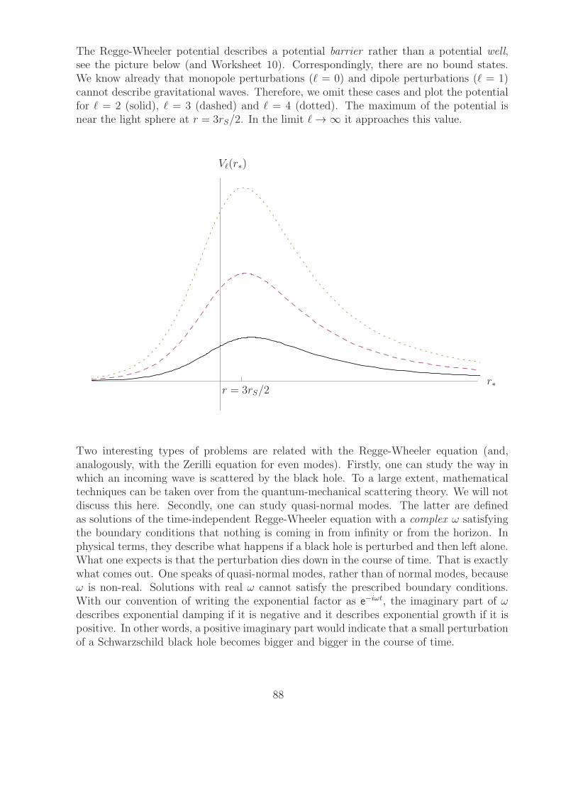
The Regge-Wheeler potential describes a potential barrier rather than a potential well,see the picture below (and Worksheet 10). Correspondingly, there are no bound states.We know already that monopole perturbations (ℓ = 0) and dipole perturbations (ℓ = 1)cannot describe gravitational waves. Therefore, we omit these cases and plot the potentialfor ℓ = 2 (solid), ℓ = 3 (dashed) and ℓ = 4 (dotted). The maximum of the potential isnear the light sphere at r = 3rS/2. In the limit ℓ → ∞ it approaches this value.
r∗
Vℓ(r∗)
r = 3rS/2
Two interesting types of problems are related with the Regge-Wheeler equation (and,analogously, with the Zerilli equation for even modes). Firstly, one can study the way inwhich an incoming wave is scattered by the black hole. To a large extent, mathematicaltechniques can be taken over from the quantum-mechanical scattering theory. We will notdiscuss this here. Secondly, one can study quasi-normal modes. The latter are definedas solutions of the time-independent Regge-Wheeler equation with a complex ω satisfyingthe boundary conditions that nothing is coming in from infinity or from the horizon. Inphysical terms, they describe what happens if a black hole is perturbed and then left alone.What one expects is that the perturbation dies down in the course of time. That is exactlywhat comes out. One speaks of quasi-normal modes, rather than of normal modes, becauseω is non-real. Solutions with real ω cannot satisfy the prescribed boundary conditions.With our convention of writing the exponential factor as e
−iωt, the imaginary part of ωdescribes exponential damping if it is negative and it describes exponential growth if it ispositive. In other words, a positive imaginary part would indicate that a small perturbationof a Schwarzschild black hole becomes bigger and bigger in the course of time.
88

More precisely, quasi-normal modes are defined as solutions Zℓm(r∗) to the time-independentRegge-Wheeler equation with a complex ω that satisfy the boundary conditions
∣∣Zℓm(r∗)− B e
−iωr∗/c∣∣ → 0 for r∗ → −∞
∣∣Zℓm(r∗)− C e
iωr∗/c∣∣ → 0 for r∗ → ∞
where B and C are any constants. These conditions mean that the function Qℓm(t, r∗) =Zℓm(r∗)e
−iωt satisfies
∣∣Qℓm(t, r∗)−B e
−iω(t+r∗/c))∣∣ → 0 for r∗ → −∞
∣∣Qℓm(t, r∗)− C e
−iω(t−r∗/c))∣∣ → 0 for r∗ → ∞ ,
i.e., that the solutions are purely ingoing (towards the horizon) for r near rS and purelyoutgoing (towards infinity) for big r. (In Worksheet 10 we discuss a bit the behaviour ofthe general solution to the Regge-Wheeler equation near the horizon and near infinity.)
Quasi-normal modes cannot be determined analytically. However, they have been exten-sively studied numerically and with the help of analytical approximation methods. Thefollowing table shows the complex frequencies for the first four quasi-normal modes forℓ = 2, 3, 4, taken from a paper by E. Leaver [“An analytic representation for the quasi-normal modes of Kerr black holes”, Proc. R. Soc. London, Ser. A, 402, 285298, (1985)].
Natural units are chosen; for conversion into Hz one has to multiply with 2π × 5142Hz×M⊙/M . We see that for fixed ℓ the real part of the frequency is maximal for the fun-damental mode (n = 0). This is in contrast to normal modes where the frequency ofthe fundamental mode is minimal. For all quasi-normal modes, the imaginary part of thefrequency is strictly negative. This demonstrates that every perturbation dies down in thecause of time, at least in the linear theory, i.e. that a Schwarzschild black hole is stableagainst linear perturbations. The damping time (i.e., the inverse of the imaginary part ofω) is surprisingly small: From the table we read that, for a black hole with a few solarmasses, the frequency is in the order of Kilohertz and the damping time is in the order ofMilliseconds!
89

The picture below shows the frequencies of the quasinormal modes of a Schwarzschild blackhole in the complex plane.
This diagram, taken from N. Andersson and S. Linnaeus [“Quasinormal modes of a Schwarz-schild black hole: Improved phase-integral treatment”, Phys. Rev. D 46, 4179, (1992)],displays the values for the quasi-normal modes with ℓ = 2 as diamonds and with ℓ = 3as crosses. A similar diagram can also be produced with the even (Zerilli) quasi-normalmodes. One finds that they lie along the same curves but at different values.
Quasi-normal modes have also been calculated for charged black holes (i.e., for the Reissner-Nordstom metric), and, with much greater difficulty, for rotating black holes (i.e., for theKerr metric). The differences could be used, in principle, for distinguishing different typesof black holes by the gravitational radiation they emit when they are perturbed.
90

8. Exact wave solutions of Einstein’s field equation
Up to now we have treated gravitational waves as perturbations of a backgroundspacetime that are so small that all equations can be linearised with respect to
them. This is a viable theory for explaining any observations that are expectedfor the foreseeable future. Nonetheless it is helpful, and even necessary for a
full understanding, to study gravitational waves at the level of the full nonlinearEinstein equation. It could well be that some of the observations made in the lin-ear theory, e.g. about the polarisation states or about the multipole characters
of gravitational waves, are just an artefact of the linearisation. In this chapterwe are going to discuss three classes of exact wave solutions to Einstein’s vac-
uum equations, known as Brinkmann solutions (or pp-waves), Einstein-Rosensolutions, and Robinson-Trautman solutions.
8.1 Brinkmann solutions (pp waves)
We begin with Minkowski spacetime in double null coordinates (x1, x2, u, v),where the u lines are the straight lightlike lines in negative x3 direction and the
v lines are the straight lightlike lines in positive x3 direction. We then modifythe spacetime in such a way that it is no longer flat but that the v lines remain
lightlike, geodesic and orthogonal to planes. The idea is that the v lines can thenbe interpreted as the “rays” of a gravitational wave with planar wave surfaces,
if the vacuum Einstein equation is satisfied.
From Minkowski spacetime in standard coordinates,
g = (dx1)2 + (dx2)2 + (dx3)2 − (dx0)2 ,
we transform to “double-null coordinates” , (x1, x2, x3, x0) 7→ (x1, x2, u, v), de-
fined by
x0 =1√2(v + u) , x3 =
1√2(v − u) .
Then
(dx0)2 − (dx3)2 =1
2
(dv + du
)2 − 1
2
(dv − du
)2=
=1
2
(du2 + 2 dv du +
dv2)− 1
2
(du2 − 2 dv du +
dv2)= 2 dv du ,
hence the Minkowski metric reads
91

g = (dx1)2 + (dx2)2 − 2 dv du .
We now add a term that makes the spacetime dynamic (time-dependent), but
in such a way that ∂v remains lightlike,
g = (dx1)2 + (dx2)2 − 2 dv du + H(x1, x2, u) du2 . (B)
with some function H(x1, x2, u). The dependence of H on u (i.e., on x0 − x3)makes the metric time-dependent. The vector field ∂u is no longer lightlike,
but the vector field ∂v still is. We will show in Worksheet 10 that, in addition,∂v is absolutely parallel, i.e., covariantly constant in any direction, hence inparticular geodesic. This allows to interpret the v lines as the propagation
direction of a wave that travels at the speed of light. Each x1-x2-surface (i.e.,each surface u = constant, v = constant) is a Euclidean plane perpendicular
to the propagation direction of the wave.
Below we will calculate the Christoffel symbols of the metric (B) from which
one can easily determine the Ricci tensor. One finds that the vacuum Einsteinequation Rµν = 0 holds if and only if H satisfies the Laplace equation with
respect to the variables x1 and x2.
δAB∂A∂BH = 0 . (T)
If the condition (T) is satisfied, the metric (B) can be interpreted as a (pure)gravitational wave. For the case that (T) is not satisfied, one finds that the
energy-momentum tensor has the form of that of an electromagnetic field; themetric can then be interpreted as a combination of a gravitational wave and anelectromagnetic wave.
Metrics of the form (B) made their first appearence in a purely mathematical
paper by H. Brinkmann [“Einstein spaces which are mapped conformally oneach other” Math. Annalen 94, 119 (1925)]. The coordinates (x1, x2, u, v) areknown as Brinkmann coordinates. A. Peres [“Some gravitational waves ” Phys.
Rev. Lett. 3, 571 (1959)] rediscovered these metrics and interpreted themas gravitational waves. They were studied in several papers by J. Ehlers and
W. Kundt [see in particular J. Ehlers and W. Kundt: “Exact solutions of thegravitational field equations” in L. Witten (ed.) “Gravitation: an introduction
to current research” Wiley, New York (1962) p.49] who called them plane-fronted
waves with parallel rays or pp-waves for short. Obviously, “plane-fronted” refersto the (x1, x2)-surfaces and “parallel rays” refers to the v-lines.
92

We will now write down the geodesic equation for the metric (B) which will giveus the Christoffel symbols. As usual, the most convenient way is to start fromthe Lagrangian
L(x, x)=
1
2gµν(x)x
µxν =1
2
(
(x1)2 + (x2)2 − 2 u v + H(x1, x2, u) u2)
where an overdot means derivative with respect to an affine parameter s. From
this we get the geodesics as the solutions to the Euler-Lagrange equation
d
ds
(
∂L(x, x)
∂xµ
)
− ∂L(x, x)
∂xµ= 0 .
Doing this for xµ = u, v and xA yields
− u = 0 ,
−v + d(H u
)
ds− 1
2∂uH u2 = 0 ,
xA − 1
2δAB∂BH u2 = 0 ,
hence
u = 0 ,
v − 1
2∂uH u2 − ∂AH u xA = 0 ,
xA − 1
2δAB∂BH u2 = 0 .
From these equations we read that the only non-vanishing Christoffel symbolsare
Γvuu = − 1
2∂uH ΓvuA = − 1
2∂AH ΓAuu = − δAB ∂BH .
From the Christoffel symbols one can calculate the Ricci tensor
Rµσ = ∂µΓττσ − ∂τΓ
τµσ + ΓρτσΓ
τµρ − ΓρµσΓ
ττρ .
One finds that the only non-vanishing component of the Ricci tensor is
Ruu =1
2δAB∂A∂BH
so that indeed the vacuum field equation Rµν = 0 is equivalent to the Laplaceequation (T), as was already anticipated above.
93

In the following we will consider those pp-waves for which the function H is aquadratic form in the variables x1 and x2,
H(x1, x2, u) = hAB(u)xAxB
with a symmetric (2× 2) matrix(hAB(u)
). If the vacuum field equation (T) is
satisfied, i.e., if the matrix(hAB(u)
)is trace-free,
δABhAB(u) = 0 ,
these special pp-waves are called plane gravitational waves ; otherwise they de-
scribe a coupled system of a plane gravitational wave and a plane electromagneticwave. Both cases were first studied by O. Baldwin and G. Jeffery [“The relativ-ity theory of plane waves”, Proc. Roy. Soc. London A 111, 95 (1926)] who did
not know about Brinkmann’s earlier work on the larger class of what we nowcall pp-waves.
The condition of vanishing trace means that for a plane gravitational wave thematrix hAB(u) can be written as
(hAB(u)
)=
(f+(u) f×(u)f×(u) − f+(u)
)
.
The profile functions f+(u) and f×(u) determine the shape of the gravitationalwave. The fact that (within the class of metrics considered) two scalar functionsare necessary to determine the wave can be interpreted by saying that “a grav-
itational wave has two polarisation states”. This is in perfect agreement withwhat we have found for plane harmonic waves in the linearised theory about
Minkowski spacetime, where we also had two polarisation states, the plus-mode
and the cross-mode).
For a plane gravitational wave the geodesic equation specifies to
u = 0 ,
v =1
2
(
f ′+(u)
((x1)2 − (x2)2)
)+ 2 f ′
×(u)x1x2)
u2
+(
f+(u)(x1x1 − x2x2
)+ f×(u)
(x1x2 + x2x1
))
u ,
(x1
x2
)
=1
2
(f+(u) f×(u)f×(u) −f+(u)
)(x1
x2
)
.
94

We see that there are geodesics that are completely contained in a lightlikehypersurface u = constant. For them we have u(s) = u0, u(s) = 0 and u(s) = 0,so the u component of the geodesic equation is satisfied. The other components
readv(s) = 0 ,
(x1(s)x2(s)
)
=1
2
(f+(u0) f×(u0)f×(u0) −f+(u0)
)(x1(s)x2(s)
)
,
which can be integrated easily.
For all the other geodesics we have u(s) 6= 0. Then the u component of thegeodesic equation, u = 0, says that u can be used as the affine parameter.
(Recall that the affine parametrisation along a geodesic is unique only up toa transformation of the form s 7→ as + b with a non-zero constant a.) With
u(s) = s, the other components of the geodesic equation read
v(s) =1
2
(
f ′+(s)
((x1(s))2 − (x2(s))2)
)+ 2 f ′
×(s)x1(s)x2(s)
)
+(
f+(s)(x1(s)x1(s)− x2(s)x2(s)
)+ f×(s)
(x1(s)x2(s) + x2(s)x1(s)
), ,
(x1(s)
x2(s)
)
=1
2
(f+(s) f×(s)f×(s) −f+(s)
)(x1(s)
x2(s)
)
.
We see that the (x1, x2) equation decouples. After having solved this equation,
v(s) is determined by a straight-forward integration. Therefore we concentrateon the matrix differential equation for x1 and x2. This equation gives the mo-
tion of the geodesics in the (x1, x2) plane, i.e., in the plane orthogonal to thepropagation direction of the wave. For the plus-mode, f× = 0, we have
(x1(s)x2(s)
)
=f+(s)
2
(x1(s)−x2(s)
)
.
At points where f+ is positive, there is focussing in the x1 direction and defo-cussing in the x2 direction; at points where f+ is negative, it is vice versa.
To discuss the cross mode, we may rotate the coordinates by 45o,(y1
y2
)
=1√2
(1 1−1 1
)(x1
x2
)
,
(x1
x2
)
=1√2
(1 −11 1
)(y1
y2
)
.
95

Then(y1
y2
)
=1√2
(1 1−1 1
)(x1
x2
)
=1√2
(1 1−1 1
)f×(s)
2
(0 11 0
)(x1
x2
)
=f×(s)
2√2
(1 1
1 −1
)1√2
(1 −1
1 1
)(y1
y2
)
=f×(s)
4
(2 0
0 −2
)(y1
y2
)
=f×(s)
2
(y1
−y2)
,
so we have the same focussing and defocussing properties as for the plus-mode,just rotated by 45o.
This consideration holds for timelike, lightlike and spacelike geodesics. For time-like geodesics it gives the motion of freely falling test particles, in analogy to what
we have discussed in the linearised theory. We see that the plus-mode and thecross-mode have the same physical interpretation for the exact plane gravita-tional waves, but now x1 and x2 may be arbitrarily large. To make the analogy
with our treatment of the linearised theory perfect, we may Fourier-expand thematrix-valued function hAB(u) (i.e., the profile functions f+(u) and f×(u)). Thenwe get exactly the same expression for each Fourier mode
hAB(u) = Reh0ABe
−iωu/c
as we had in the linearised theory.
We now turn to the lightlike geodesics. The
picture on the right shows the past light-coneof an event R, in a famous hand-drawing by
Roger Penrose [“ A remarkable property ofplane waves in general relativity” Rev. Mod-
ern Phys. 37, 215 (1965)]. One sees that,with the exception of the v-line through R(which is a straight line), all light rays that
are issuing from the eventR into the past arerefocussed into another event Q. Actually,
taking the fourth dimension into account which is missing in the picture, a
pure gravitational wave refocusses light rays into a line (“astigmatic focussing”).A combined gravitational and electromagnetic wave can refocus light rays intoa point (“anastigmatic focussing”). The picture also indicates that a plane-
wave spacetime cannot admit a Cauchy hypersurfaces, i.e., a hypersurface thatintersects any causal curve exactly once: Such a hypersurface would have to
intersect the v-line through R. But then some of the other past-oriented lightlikegeodesics from R to Q have to be intersected twice.
96

The following picture of the light cone was produced with Mathematica. Theprofile functions were chosen as f×(u) = 0 and f+(u) = k2χ(u), where k is a non-zero constant and χ(u) is the characteristic function of a finite interval (i.e., the
gravitational wave is “sandwiched“ between two flat spacetime regions, boundedby hypersurfaces u = constant). The x2 dimension is omitted. The similarity
with the Penrose drawing is striking.
x1
uu
u
vv
v
++
−
The picture on the right gives a purely
spatial view of the light-cone above. Nowboth spatial dimensions x1 and x2 are
shown and the temporal dimension, u+v,is omitted. One clearly sees the astig-
matic focussing: There is focussing in onespatial dimension and defocussing in theother spatial dimension, so that the light-
like geodesics are refocussed in a line.
97

8.1 (Beck-)Einstein-Rosen solutions
In this section we want to discuss a class of excact wave-like solutions to Ein-
stein’s vacuum equation with cylindrical symmetry. These solutions are usuallycalled Einstein-Rosen waves although they were found by Austrian physicist
Guido Beck already 12 years before Einstein and Rosen [G. Beck: “Zur Theoriebinarer Gravitationsfelder” Zeitschr. f. Physik 33, 713 (1925)].
Beck started out from known results on axisymmetric and static metrics whichhad been found by H. Weyl in 1917. A metric is axisymmetric and static if
it can be written in cylindrical polar coordinates (t, ρ, ϕ, z) such that the gµνare independent of t, independent of ϕ, and invariant under a transformation
ϕ 7→ −ϕ. Such metrics describe the gravitational fields of time-independent non-rotating bodies with axial symmetry. (If the invariance under the transformation
ϕ 7→ −ϕ is dropped one speaks of axisymmetric stationary metrics; then rotatingbodies are included.) Beck took the known axisymmetric and static metrics andperformed the formal substitution t 7→ iz, z 7→ it. Then the metric is still
axisymmetric but, instead of being time-independent, it is now invariant undertranslations in z-direction. In this way one gets time-dependent metrics (waves)
with cylindrical symmetry.
The ansatz for the metric reads
gµνdxµdxν = e
2γ−2ψ(dρ2 − c2dt2
)+ e
−2ψW 2dϕ2 + e2ψdz2
where γ, ψ and W are functions of t and ρ. This is precisely the same ansatz,
with the above-mentioned substitution, as it is used for the axisymmetric andstatic metrics; in the latter context, one speaks of Weyl canonical coordinates.
This is the most general form of a cylindrically symmetric metric apart fromthe fact that we have assumed invariance under ϕ 7→ −ϕ (in analogy to the
axisymmetric static case). Note that the ansatz of the metric in the (t, ρ) planebeing proportional to
(dρ2 − c2dt2
)is no restriction as every two-dimensional
metric is conformal to the flat metric.
To find vacuum solutions with the prescribed symmetry we have to calculate
the Ricci tensor. As usual, the easiest way to find the Christoffel symbols is bystarting from the Lagrangian for the geodesics,
L(xx) =1
2
(
e2γ−2ψ
(ρ2 − c2t2
)+ e
−2ψW 2ϕ2 + e2ψz2
)
where the overdot means differentiation with respect to an affine parameter s.The Euler-Lagrange equations give the four components of the geodesic equation.
98

After some elementary algebra they take the following form.
z + 2 ∂ρψ ρ z + 2 ∂tψ t z = 0 ,
ϕ+ 2(∂ρW
W− ∂ρψ
)
ρ ϕ+ 2(∂tW
W− ∂tψ
)
t ϕ = 0 ,
ρ+(∂ργ − ∂ρψ
)ρ2 − 2
(∂tγ − ∂tψ
)ρ t+
(∂ργ − ∂ρψ
)c2t2
−e−2γW 2
(∂ρW
W− ∂ρψ
)
ϕ2 − e−2γ+4ψ∂ρψ z
2 = 0 ,
t+ 2(∂ργ − ∂ρψ
)ρ t+
(∂tγ − ∂tψ
)t2 +
(∂tγ − ∂tψ
) 1
c2ρ2
+e−2γW
2
c2
(∂tW
W− ∂tψ
)
ϕ2 + e−2γ+4ψ∂tψ
1
c2z2 = 0 .
From these equations we can read the Christoffel symbols and, thereupon, cal-culate the Ricci tensor. We find
Rzz = e−2γ+4ψ
(
∂2ρψ − 1
c2∂2tψ +
∂ρW
W∂ρψ − ∂tW
c2W∂tψ)
,
Rϕϕ = W 2e−2γ(
− ∂2ρψ +1
c2∂2tψ +
∂2ρW
W− ∂2tW
c2W− ∂ρW
W∂ρψ +
∂tW
c2W∂tψ)
,
Rtt = ∂2t γ − c2∂2ργ − ∂2tψ + c2∂2ρψ +∂2tW
W− c2
∂ρW
W
(∂ργ − ∂ρψ
)
−∂tWW
(∂tγ + ∂tψ
)+ 2(∂tψ)2,
Rρρ = ∂2ργ − 1
c2∂2t γ − ∂2ρψ +
1
c2∂2tψ +
∂2ρW
W− ∂ρW
W
(∂ργ + ∂ρψ
)
−∂tWc2W
(∂tγ − ∂tψ
)+ 2(∂ρψ)2,
Rρt = Rtρ =∂ρ∂tW
W− ∂ρW
W∂tγ − ∂tW
W∂ργ + 2∂ρψ ∂tψ ,
99

The other components of the Ricci tensor are zero. This reduces the vacuumfield equation to five scalar equations. The first two equations, Rzz = 0 andRϕϕ = 0, are equivalent to the two equations
∂2ρW − 1
c2∂2tW = 0 , (B1)
∂2ρψ − 1
c2∂2tψ +
∂ρW
W∂ρψ − ∂tW
c2W∂tψ = 0 . (B2)
Similarly, the equations Rρρ = 0 and Rtt = 0 are equivalent to the two equations
∂2tW
2c2W+∂2ρW
2W− ∂ρW
W∂ργ − ∂tW
c2W∂tγ +
1
c2(∂tψ)2
+(∂ρψ)2
= 0 , (B3)
∂2ργ − 1
c2∂2t γ − 1
c2(∂tψ)2
+(∂ρψ)2
= 0 . (B4)
The last component requires
∂ρ∂tW
W− ∂ρW
W∂tγ −
∂tW
W∂ργ + 2∂ρψ ∂tψ = 0 . (B5)
We will solve these equations for two cases.
Case A :(∂ρW
)2 − 1
c2(∂tW
)2> 0
This condition, which says that the gradient of the functionW is spacelike,guarantees, in particular, that this gradient has no zeros. We can, therefore,
useρ = W (t, ρ)
as a new coordinate. We use this freedom for performing a coordinatetransformation (t, ρ) 7→
(t, ρ)such that
dt = ∂ρW dt+∂tW
c2dρ , dρ = ∂ρW dρ+ ∂tW dt .
The second equation is just the differential version of the definition of ρ.
We have to check if the first equation defines, indeed, a function t. Theequations
∂tt = ∂ρW , ∂ρt =∂tW
c2
can be satisfied only if the integrability condition
∂2ρW =∂2tW
c2
100
is satisfied. This, however, is guaranteed by the field equation, see (B1).Our new coordinates satisfy
dρ2 − c2dt2 =(
∂ρW dρ+ ∂tW dt)2
− c2(
∂ρW dt+∂tW
c2dρ)2
=((∂ρW
)2 − 1
c2(∂tW
)2)(dρ2 − c2dt2
).
Note that the factor on the right-hand side is positive by assumption. There-
fore, we can replace the function γ by a new function γ, defined by
e2γ =
e2γ
(∂ρW
)2 − 1
c2(∂tW
)2.
Then the metric reads
gµνdxµdxν = e
2γ−2ψ(dρ2 − c2dt2
)+ e
−2ψρ2dϕ2 + e2ψdz2 .
In the following we drop the tildas. Now we have to evaluate our fieldequations (B1) to (B5) with W (t, ρ) = ρ. (B1) is automatically satisfied.
(B2) becomes
∂2ρψ +1
ρ∂ρψ − 1
c2∂2tψ = 0 . (B2’)
(B3) and (B5) can be solved for the partial derivatives of γ,
∂ργ = ρ((∂ρψ)2
+1
c2(∂tψ)2)
, (B3’)
∂tγ = 2 ρ ∂ρψ ∂tψ . (B5’)
(B4) is then automatically satisfied. Note that (B2’) is a differential equa-tion for ψ alone. We can solve this equation with a standard separationansatz. After splitting off the time part we are left with the radial part
of the Laplace equation in cylindrical coordinates which is the well-knownBessel equation. Therefore the general solution to (B2’) is
ψ(t, ρ) = AJ0(ωρ) cos(ωt) +B Y0(ωρ) sin(ωt)
where J0 and Y0 are the Bessel functions of first and second kind, respec-
tively. While J0 is regular everywhere, Y0 goes to −∞ for ρ → 0. If wewant to have a solution that is regular on the axis we have to choose B = 0.Having solved (B2’), we can determine γ from (B3’) and (B5’). It is obvious
101
that the solution γ is unique up to an additive constant. Existence of thesolution is less trivial. We have to check if the integrability condition issatisfied:
∂t
ρ((∂ρψ)2
+1
c2(∂tψ)2)
?= ∂ρ
2 ρ ∂ρψ ∂tψ
,
ρ(
2∂ρψ ∂t∂ρψ +
2
c2∂tψ∂
2t ψ)
?= 2 ∂ρψ ∂tψ + 2 ρ ∂2ρψ ∂tψ +(((((((((
2 ρ ∂ρψ ∂ρ∂tψ ,
0!= 2 ρ ∂tψ
(1
ρ∂ρψ + ∂2ρψ − 1
c2∂2tψ
)
.
We see that the integrability condition of (B3’) and (B5’) is just the equa-
tion (B2’). This guarantees that to every solution of (B2’) we find a cor-responding γ such that all components of the vacuum field equation aresatisfied.
This class of solutions describes gravitational waves with cylindrical sym-
metry. For B = 0 they are well-defined, as source-free vacuum solutions,on all of R4. There is a coordinate singularity on the axis, as always when
using cylindrical polar coordinates, but no curvature singularity. This classof vacuum solutions was (re-)discovered by A. Einstein and N. Rosen [“On
gravitational waves” J. Franklin Inst. 223, 43 (1937)]. In an earlier ver-sion of this paper, Einstein and Rosen had interpreted the coordinate wecalled ϕ as a non-periodic, Cartesian-like coordinate and, correspondingly,
the waves as planar rather than as cylindrical. The (coordinate) singularityat ρ = 0 gave them the impression that this solution is unphysical and they
even concluded from this observation that gravitational waves do not existin the full non-linear theory. Einstein and Rosen submitted their paper
with this (completely false) conclusion to Physical Review. The Editor sentthe article to a referee (which had never been happened to Einstein before)
who pointed out that the conclusion was erroneous and that, actually, thesolutions are cylindrical. Einstein was so angry about the fact that his ar-ticle had been sent for refereeing that he withdraw the paper and decided
never again to publish in Physical Review. After H. P. Robertson (who, aswe know now, was the referee) explained to him his error, Einstein wrote
a completely new version of the article (N. Rosen had left for Russia bythat time) which was then published in the Journal of the Franklin Insti-
tute. The cylindrical solutions presented in this paper are now known asEinstein-Rosen waves although they had already been found by Beck 12years earlier.
102

Case B :(∂ρW
)2 − 1
c2(∂tW
)2= 0 , ∂ρW 6= 0
This condition says that the gradient of the function W is lightlike andnon-zero. Then we have
∂ρW = ±1
c∂tW .
Here and in the following, either the upper sign or the lower sign holds.The components (B3) and (B5) of the field equations read
∂2ρW
W− ∂ρW
W∂ργ ∓ ∂ρW
cW∂tγ +
1
c2(∂tψ)2
+(∂ρψ)2
= 0 ,
∂2ρW
W∓ ∂ρW
cW∂tγ − ∂ρW
W∂ργ ± 2
c∂ρψ∂tψ = 0 .
Subtracting the second equation from the first yields
∂ρψ = ±1
c∂tψ ,
i.e.,ψ(t, ρ) = f(ct± ρ) .
Upon inserting this result into (B4), and using that ∂ρW has no zeros, wefind
∂2ργ −1
c2∂2t γ = 0 ,
i.e.,γ(t, ρ) = p(ct± ρ) + q(ct∓ ρ) .
With these results our metric takes the form
gµνdxµdxν = −
(
e2p−2f(cdt± dρ))(
e2q(cdt∓ dρ))
+ e−2fW 2dϕ2 + e2fdz2 .
We replace t and ρ by new coordinates(u, v)such that
du =1√2e2p−2f(cdt± dρ) , dv =
1√2e2q(cdt∓ dρ) .
This is possible as the integrability conditions are obviously satisfied. Thenthe metric reads
gµνdxµdxν = 2dudv + C11(u)dϕ
2 + C22(u)dz2
103

where we have used that f and W depend on t± ρ only which, in turn, canbe expressed in terms of u alone. Metrics of the form
gµνdxµdxν = −2dudv + CAB(u)dx
AdXB
are known as Rosen waves. They were discussed in a paper by N. Rosenwhich he wrote after he had left Princeton for the Soviet Union [N. Rosen:“Plane polarized waves in the general theory of relativity”. Phys. Z. Soviet
Union 12, 366 (1937)]. With our metric ansatz we have found only thoseRosen waves for which the matrix CAB(u) is diagonal; one gets the general
class if one drops the assumption of the ϕ lines being orthogonal to the zlines.
The Rosen waves are actually locally isometric to the plane waves we havestudied in the preceding section in the Brinkmann coordinates. We demon-
strate this for the case that the matrix CAB is diagonal.
We start out from the metric in Rosen coordinates with
(CAB
)=
(e1(u
2)2 00 e2(u
2)2
)
.
We express the Rosen coordinates(u, v, x1, x2
)in terms of new coordinates
(which will turn out to be the Brinkmann coordinates) (u, v, x1, x2) by
u = u , v = v − 1
2
( e1(u)
e1(u)(x1)2 +
e2(u)
e2(u)(x2)2
)
,
x1 =x1
e1(u), x2 =
x2
e2(u).
Thengµνdx
µdxν = −2dudv + e21(dx1)2
+ e22(dx2)2
= −2du
dv− 1
2
e1e12x1dx1 − 1
2
e2e22x2dx2 − 1
2
( e1e1
)·(x1)2du+
1
2
( e2e2
)·(x2)2du
+e21
(dx1
e1− e1e21x1du
)2
+ e22
(dx2
e2− e2e22x2du
)2
= −2dudv + dudx1
2e1e1x1 −
2e1e1x1)
+ dudx2(
2e2e2x2 −
2e2e2x1
+du2( e1
e1−
e21e21
)
(x1)2+( e1e2−
e22e22
)
(x2)2+
e21
e21(x1)2+
e22
e22(x2)2
)
+(dx1)2+(dx2)2 .
104

This is precisely the form of a plane wave in Brinkmann coordinates,
gµνdxµdxν = −2dudv + hAB(u)x
AxBdu2 + (dx1)2 + (dx2)2 ,
with
(hAB(u)
)=
e1(u)
e10
0e2(u)
e2
.
The vacuum field equation requires
e1(u)
e1+e2(u)
e2= 0 .
The other cases, where the gradient of W is timelike, or where it changes its
causal character from point to point, will not be treated here. The latter case isof relevance for colliding waves.
8.3 Robinson-Trautman solutions
While plane waves are associated with bounded sources only approximately,at a large distance from the sources, and cylindrical waves are not associated
with bounded sources at all, we will finally study a class of solutions that dogive a valid description of gravitational radiation from bounded sources. It was
constructed by I. Robinson and A. Trautman [“Some spherical gravitationalwaves in general relativity” Proc. Roy. Soc. London A 265, 463 (1962)] in
analogy to the Lienard-Wiechert field from electrodynamics. The latter is theelectromagnetic field of an accelerated point charge in Minkowski spacetime.
The radiation field propagates along the lightlike geodesics (i.e., lightlike straightlines) that issue from the worldline of the point charge into the future. Theselightlike geodesics, which generate the future light-cones from the events of the
worldline of the charge, are hypersurface-orthogonal, shear-free and expanding.The basic idea of Robinson and Trautman was to construct vacuum solutions
to Einstein’s field equation which admit a family of lightlike geodesics with thesame properties. One could then interpret these lightlike geodesics as the rays
of gravitational radiation.
We begin by writing down the general form of a spacetime that is foliated into
lightlike hypersurfaces. These hypersurfaces, which generalise the light-cones in
105

Minkowski spacetime, can be written as hypersurfaces σ = constant where σ isa scalar function with a lightlike gradient,
gµν∂µσ∂νσ = 0 .
We define a vector field Kµ∂µ by
Kµ = gµν∂νσ .
Clearly, this vector field is lightlike,
gµνKµKν = gµνg
µρ∂ρσgνλ∂λσ = gρλ∂ρσ∂λσ = 0 ,
and geodesic,
0 = gµν∂µσ∂νσ =⇒ 0 = ∇λ
(gµν∂µσ∂νσ
)= 2gµν∂µ∇λ∂νσ
= 2Kν(∂λ∂νσ − Γτ λνσ
)= 2Kν
(∂ν∂λσ − Γτ νλσ
)= 2Kν∇ν∂λσ = 2Kν∇νKλσ .
Note that the vector field Kµ∂µ is tangent to the hypersurfaces σ = constantand at the same time orthogonal to them.
∂1, ∂2
∂3
∂4
σ = constant
We can choose coordinates x1 = ξ, x2 = η, x3 = ρ and x4 = σ in such a waythat
∂
∂ρ= ∂3 = Kµ∂µ .
This can be achieved by assigning the value ρ = ρ0 to a hypersurface that istransverse to the hypersurfaces σ = constant and dragging it along with the
106

flow of Kµ∂µ to get the other hypersurfaces ρ = constant; the coordinates ξand η have to be chosen transverse to σ, but arbitrarily otherwise, on the initialhypersurface ρ = ρ0 and are then again fixed by dragging them along with the
flow of Kµ∂µ. By construction,
g14 = g41 = gµνδ4µδ1ν = gµν∂µσ∂νξ = Kν∂νξ =
∂ξ
∂ρ= 0 ,
g24 = g42 = gµνδ4µδ2ν = gµν∂µσ∂νη = Kν∂νη =
∂η
∂ρ= 0 ,
g34 = g43 = gµνδ4µδ3ν = gµν∂µσ∂νρ = Kν∂νρ =
∂ρ
∂ρ= 1 ,
g44 = gµνδ4µδ4ν = gµν∂µσ∂νσ = 0 .
This demonstrates that the contravariant components of the metric can be writ-ten as
(gµν)=
P 2γ11 P 2γ12 a 0P 2γ12 P 2γ22 b 0
a b c 10 0 1 0
with det
(γ11 γ12
γ12 γ22
)
= 1 .
Here we have used that the two-surfaces parametrised by ξ and η are spacelike, so
the determinant of(gAB
)must be positive. (As before, capital indices A,B, . . .
take values 1 and 2.) From the minors of the matrix (gµν) we read that g31 =g32 = g33 = 0, hence
δBA = gAµgµB = gACg
CB = gACP2γCB =⇒ (γ−1)AC = P 2gAC .
We will now add the condition that Kµ∂µ should be shear-free and expanding.Twist, expansion and shear of the lightlike vector field Kµ∂µ are defined as
twist : ΩAB =1
2
(∇AKB −∇BKA
),
expansion : Θ = ∇AKA ,
shear : ΣAB =1
2
(∇AKB +∇BKA
)− Θ
2gAB .
In the case at hand,
∇µKν = ∇µ∂νσ = ∂µ∂νσ − Γλµν∂λσ = 0− 1
2gλτ(∂µgτν + ∂νgτµ − ∂τgµν
)δ4λ
107

= −1
2g43︸︷︷︸=1
(∂µ g3ν︸︷︷︸=0
+ ∂ν g3µ︸︷︷︸=0
− ∂3gµν)=
1
2∂3gµν .
Hence, the twist vanishes, ΩAB = 0. (Quite generally, the property of being
hypersurface-orthogonal is equivalent to being twist-free.) To calculate the ex-pansion, we observe that the Jacobi formula
∂3(det(γ)
)= trace
(γ−1∂3γ
)
applied to the matrix γ = (γAB) results in
0 =(γ−1)
AB∂3γ
AB ,
hence
Θ = gAB∇AKB =1
2gAB∂3gAB = −1
2gAB∂3g
AB = −1
2P−2(γ−1)AB∂3(P
2γAB)
= −1
2P−2(γ−1)ABγ
AB2P∂3P = −2P−1∂3P .
Finally, we find the shear as
ΣAB =1
2∂3gAB + P−1∂3PgAB =
1
2∂3(P−2(γ−1)AB
)+ P−3(γ−1)AB∂3P
=1
2P−2∂3
((γ−1)AB
).
We assume that the shear vanishes, i.e., that ∂3((γ−1)AB
)= 0. This condition is
equivalent to ∂3γAB = 0. If we choose the coordinates ξ and η such that γAB =
δAB on the initial hypersurface ρ = ρ0, this condition will hold everywhere, sothe contravariant components of the metric simplify to
(gµν)=
P 2 0 a 0
0 P 2 b 0a b c 1
0 0 1 0
.
This matrix can be easily inverted,
(gµν)=
P−2 0 0 −P−2a
0 P−2 0 −P−2b0 0 0 1
−P−2a −P−2b 1 −c+ P−2a2 + P−2b2
,
108

so the metric reads
gµνdxµdxν = P−2
((dξ − a dσ
)2+(dη − b dσ
)2)
+ 2 dρ dσ − c dσ2 .
This is the general form of a metric that admits a hypersurface-orthogonal,
shear-free geodesic lightlike vector field.
Finally, we add the conditions that the expansion is non-zero and that the vac-
uum field equation Rµν = 0 holds. We begin with the 33-component of the fieldequation.
0 = R33 = RτµτνK
µKν = Kµ(∇µ∇τK
τ −∇τ∇µKτ)
= Kµ∇µ∇τKτ −∇τ
(Kµ∇µK
τ
︸ ︷︷ ︸=0
)+∇µK
µ∇τKτ
= ∂3(∇AK
A + 0)+∇AK
B∇BKA + 0 = ∂3Θ+
1
4gBCgAD∂3gAC∂3gBD
= ∂3Θ+P 4
4δBCδAD∂3
(P−2δAC
)∂3(P−2δBD
)
= ∂3Θ+P 4
4
(−2P−3∂3P︸ ︷︷ ︸
=P−2Θ
)2δBAδ
AB︸ ︷︷ ︸
=2
=∂Θ
∂ρ+
Θ2
2.
Quite generally, evaluating the expression RµνKµKν results in a differential
equation for the expansion Θ along the integral curves of Kµ∂µ which is known
as the Raychudhuri equation. In the case at hand, assuming R33 = 0, it simplyreads
∂Θ
∂ρ=
Θ2
2.
Now we use our assumption that Θ 6= 0. Then we can integrate the Raychudhuriequation,
− 2
Θ2
∂Θ
∂ρ= 1 =⇒ 2
∂Θ−1
∂ρ= 1 =⇒ 2
Θ= ρ+ f(ξ, η, σ) .
As ρ was introduced by assigning a value ρ0 to an arbitrary hypersurface trans-
verse to the lightlike hypersurfaces σ = constant, we are free to make a coordi-nate transformation ρ 7→ ρ− f(ξ, η, σ). Then we have
ρ =2
Θ= −P
(∂P
∂ρ
)−1
=⇒ ∂P
∂ρ= −P
ρ
109

=⇒ ∂(ρP)
∂ρ= P + ρ
∂P
∂ρ= P − ρ
P
ρ= 0 .
So our assumption that (at least the 33-component of) the vacuum field equationholds and that Θ 6= 0 has led to the conclusion that
p := ρP satisfies∂p
∂ρ= 0 .
So we can write the metric as
gµνdxµdxν =
ρ2
p2
((dξ−a dσ
)2+(dη−b dσ
)2)
+2 dρ dσ−c dσ2 with ∂3p = 0 .
For evaluating the vacuum field equation, we now have to calculate the other
components of the Ricci tensor for this metric. This is straight-forward butrather tedious. Mathematica gives the following results.
R13 =∂3(ρ
4∂3a)
2p2ρ2,
R23 =∂3(ρ
4∂3b)
2p2ρ2,
R11 − R22 =ρ
2p4
(
ρ2(∂3a)2 − ρ2(∂3b)
2 − 2p2(2∂2b+ ρ∂2∂3b− 2∂1a− ρ∂1∂3a
))
,
R2 =ρ
2p4
(
ρ2∂3a ∂3b+ p2(2∂2a+ ρ∂2∂3a+ 2∂1b+ ρ∂1∂3b
))
.
The first two and the last two equations can be combined in complex form,
respectively, if we introduce the complex function z := a+ ib,
R13 + iR23 =∂3(ρ
4∂3z)
2p2ρ2,
R11 −R22 + 2iR12 =ρ
2p4
(
ρ2(∂3z)2 + 2p2
(∂1 + i∂2
)(2z + ρ∂3z
))
.
The vacuum field equation requires R13 + iR23 = 0, hence
ρ4∂3z = v =⇒ z = u− v
3ρ3with ∂3u = ∂3v = 0 .
Inserting this result into the equation R11 − R22 + 2iR12 = 0 yields
0 = v2 + 2p2(∂1 + i∂2
)(2uρ6 +
v
3ρ3).
110

By comparing equal powers of ρ we find
v = 0 and (∂1 + i∂2)u = 0 ,
i.e., the function z = a + ib = u is independent of ρ = x3 and analytic in the
complex variable ξ + iη = x1 + ix2,
∂3z = 0 , (∂1 + i∂2)z = 0 .
The second condition means that, if real and imaginary parts are written sepa-rately, the Cauchy-Riemann equations
∂a
∂ξ=∂b
∂η,
∂a
∂η= −∂b
∂ξ
hold.
On the basis of these observations we will now show that a and b can be trans-formed to zero. To that end we perform a coordinate transformation of the
form
ξ = α(ξ, η, σ) , η = β(ξ, η, σ) , σ = γ(σ) , ρ =ρ
γ ′(σ)
where α + iβ is an analytic function of ξ + iη, i.e.,
∂α
∂ξ=∂β
∂η,
∂α
∂η= −∂β
∂ξ.
We choose α and β such that
aγ ′(σ) =∂α
∂σ, bγ ′(σ) =
∂β
∂σ.
Such a choice is possible because a and b are independent of ρ and satisfy the
Cauchy-Riemann equations, which guarantees that the necessary integrabilityconditions are satisfied,
∂
∂ξ(a γ ′(σ)) = γ ′(σ)
(∂a
∂ξ
∂α
∂ξ+∂a
∂η
∂β
∂ξ
)
= γ ′(σ)
(∂b
∂η
∂β
∂η+∂b
∂ξ
∂α
∂η
)
=∂
∂η(b γ ′(σ)) ,
∂
∂η(a γ ′(σ)) = γ ′(σ)
(∂a
∂ξ
∂α
∂η+∂a
∂η
∂β
∂η
)
= γ ′(σ)
(∂b
∂η
∂β
∂ξ+∂b
∂ξ
∂α
∂ξ
)
=∂
∂ξ(b γ ′(σ)) .
Under such a transformation the form of the metric is preserved, with
1
p2=
1
p2
((∂α
∂ξ
)2
+(∂β
∂ξ
)2)
=1
p−2
((∂α
∂η
)2
+(∂β
∂η
)2)
111

a = 0 , b = 0 , c = cγ ′(σ)2 .
If we perform such a coordinate transformation, and then drop the tildas, the
metric takes the simple form
gµνdxµdxν =
ρ2
p2(dξ2 + dη2
)+ 2 dρ dσ − c dσ2 (RT)
with functions p(ξ, η, σ) and c(ξ, η, ρ, σ).
For this metric we now calculate the remaining components of the Ricci tensor.
Again with Mathematica, we find
R11 + R22 =2
p
(
∂3(ρc)− 4ρ ∂4ln p−∆ln p)
where we introduced the modified Laplace operator
∆ = p2(∂21 + ∂22
).
Integration of the equation R11 + R22 = 0 yields
c = 2ρ∂4ln p+∆ln p− 2m
ρwith ∂3m = 0 . (∗)
With this input we find that R34 = 0 is satisfied while
R14 =∂1m
ρ2, R24 =
∂2m
ρ2.
Hence, the equations R14 = 0 and R24 = 0 require m to be a function of σ only.
Finally, the remaining component of the Ricci tensor is
R44 =1
2ρ2
(
∆2 ln p + 12m∂4ln p− 4dm
dσ
)
.
The condition R44 = 0 gives a fourth-order differential equation for p which isknown as the Robinson-Trautman equation,
∆2ln p + 12m∂4ln p− 4dm
dσ= 0 .
We can now summarise the procedure of how to construct a Robinson-Trautman
vacuum solution. We choose a function m(σ). With this function, we have tofind a solution p to the Robinson-Trautman equation. With this p and thechosen m, we define a function c via (∗). Then the metric (RT) is a solution to
112

Einstein’s vacuum equation with the integral curves of ∂/∂ρ being a twist-free,shear-free, geodesic lightlike congruence with non-zero expansion.
Clearly, the Schwarzschild solution must be included. To verify this, choose form a positive constant. Then the Robinson-Trautman equation is solved by
p = 1 +1
4
(ξ2 + η2
),
because
∂4ln p = 0 , ∆ln p = 1 .
In this case the function c reads
c = ∆ln p− 2m
ρ= 1− 2m
ρ.
We express the coordinates ξ and η in terms of new coordinates ϑ and ϕ via
ξ + iη = 2 tanϑ2eiϕ
which is the stereographic projection mapping from a sphere to a plane. Then
dξ2 + dη2 =4 sin2ϑ
2cos2ϑ
2dϕ2 + dϑ2
cos4ϑ2
=sin2ϑ dϕ2 + dϑ2
cos4ϑ2
,
p = 1 +1
4
(ξ2 + η2
)= 1 + tan2ϑ
2=
1
cos2ϑ2
,
so the metric reads
gµνdxµdxν = ρ2
(sin2ϑ dϕ2 + dϑ2
)+ 2dρdσ −
(
1− 2m
ρ
)
dσ2 .
If we rename (ρ, σ) 7→ (r,±ct) we recognise the Schwarzschild metric in ingoingand outgoing Eddington-Finkelstein coordinates, respectively.
The Robinson-Trautman class of solutions also contains the socalled C-metric
which describes a uniformly accelerated black hole. It can be viewed as thegravitational analogue of the Born-Schott electromagnetic field produced by a
uniformly accelerated charge. Just as an accelerated charge produces station-
ary electromagnetic radiation, the C-metric describes stationary gravitational
radiation.
Other Robinson-Trautman solutions describe non-stationary gravitational ra-diation produced by bounded sources. At the level of exact solutions to Ein-stein’s field equation, the Robinson-Trautman metrics are the most realistic
113

models of gravitational radiation we have. As they do not include any (over-idealised) symmetry assumptions, their variety is much richer than that ofthe Brinkmann or (Beck-)Einstein-Rosen solutions. For a detailed discussion
of Robinson-Trautman metrics, including the C-metric, see J. Griffiths and J.Podolsky: “Exact Space-Times in General Relativity” Cambridge University
Press, 2009.
There are several generalisations of the Robinson-Trautman solutions. In par-ticular, the condition of the rays being hypersurface-orthogonal (twist-free) has
been dropped. This is important to include rotating sources. A twisting nullcongruence can be rather complicated. In Roger Penrose’s twistor formalism any
twistor is associated with a certain twisting, shear-free, geodesic null congruence,called a “Robinson congruence”, on (complexified, compactified) Minkowskispacetime. The picture below is a hand-drawing by Roger Penrose. It shows
a time-slice of a Robinson congruence.
114