Full Terms & Conditions of access and use can be found athttp://www.tandfonline.com/action/journalInformation?journalCode=ujrs20

Download by: [134.117.247.192] Date: 13 February 2017, At: 07:42

Canadian Journal of Remote SensingJournal canadien de télédétection

ISSN: 0703-8992 (Print) 1712-7971 (Online) Journal homepage: http://www.tandfonline.com/loi/ujrs20

Effect of Different Grazing Intensities on theSpatial-Temporal Variability in Above-GroundLive Plant Biomass in North American MixedGrasslands

Ravinder Virk & Scott W. Mitchell

To cite this article: Ravinder Virk & Scott W. Mitchell (2014) Effect of Different GrazingIntensities on the Spatial-Temporal Variability in Above-Ground Live Plant Biomass in NorthAmerican Mixed Grasslands, Canadian Journal of Remote Sensing, 40:6, 423-439, DOI:10.1080/07038992.2014.1009882

To link to this article: http://dx.doi.org/10.1080/07038992.2014.1009882

Accepted author version posted online: 28Jan 2015.Published online: 28 Jan 2015.

Submit your article to this journal

Article views: 150

View related articles

View Crossmark data

Canadian Journal of Remote Sensing, 40:423–439, 2014Copyright c© CASIISSN: 0703-8992 print / 1712-7971 onlineDOI: 10.1080/07038992.2014.1009882

Effect of Different Grazing Intensitieson the Spatial-Temporal Variability in Above-GroundLive Plant Biomass in North American Mixed Grasslands

Ravinder Virk1,*, and Scott W. Mitchell21Department of Geography, University of Lethbridge, Lethbridge, Alberta, T1K 3M4, Canada2Department of Geography and Environmental Studies, Geomatics and Landscape Ecology Laboratory,Carleton University, Ottawa, Ontario, K1S 5B6, Canada

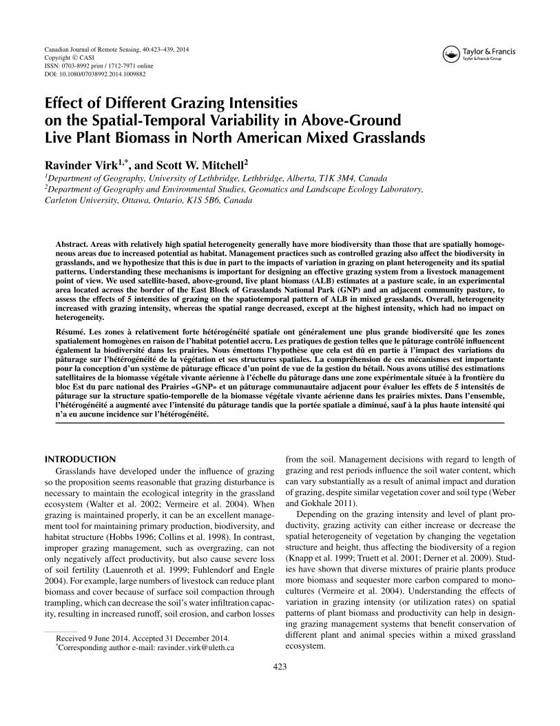
Abstract. Areas with relatively high spatial heterogeneity generally have more biodiversity than those that are spatially homoge-neous areas due to increased potential as habitat. Management practices such as controlled grazing also affect the biodiversity ingrasslands, and we hypothesize that this is due in part to the impacts of variation in grazing on plant heterogeneity and its spatialpatterns. Understanding these mechanisms is important for designing an effective grazing system from a livestock managementpoint of view. We used satellite-based, above-ground, live plant biomass (ALB) estimates at a pasture scale, in an experimentalarea located across the border of the East Block of Grasslands National Park (GNP) and an adjacent community pasture, toassess the effects of 5 intensities of grazing on the spatiotemporal pattern of ALB in mixed grasslands. Overall, heterogeneityincreased with grazing intensity, whereas the spatial range decreased, except at the highest intensity, which had no impact onheterogeneity.

Resume. Les zones a relativement forte heterogeneite spatiale ont generalement une plus grande biodiversite que les zonesspatialement homogenes en raison de l’habitat potentiel accru. Les pratiques de gestion telles que le paturage controle influencentegalement la biodiversite dans les prairies. Nous emettons l’hypothese que cela est du en partie a l’impact des variations dupaturage sur l’heterogeneite de la vegetation et ses structures spatiales. La comprehension de ces mecanismes est importantepour la conception d’un systeme de paturage efficace d’un point de vue de la gestion du betail. Nous avons utilise des estimationssatellitaires de la biomasse vegetale vivante aerienne a l’echelle du paturage dans une zone experimentale situee a la frontiere dubloc Est du parc national des Prairies «GNP» et un paturage communautaire adjacent pour evaluer les effets de 5 intensites depaturage sur la structure spatio-temporelle de la biomasse vegetale vivante aerienne dans les prairies mixtes. Dans l’ensemble,l’heterogeneite a augmente avec l’intensite du paturage tandis que la portee spatiale a diminue, sauf a la plus haute intensite quin’a eu aucune incidence sur l’heterogeneite.

INTRODUCTIONGrasslands have developed under the influence of grazing

so the proposition seems reasonable that grazing disturbance isnecessary to maintain the ecological integrity in the grasslandecosystem (Walter et al. 2002; Vermeire et al. 2004). Whengrazing is maintained properly, it can be an excellent manage-ment tool for maintaining primary production, biodiversity, andhabitat structure (Hobbs 1996; Collins et al. 1998). In contrast,improper grazing management, such as overgrazing, can notonly negatively affect productivity, but also cause severe lossof soil fertility (Lauenroth et al. 1999; Fuhlendorf and Engle2004). For example, large numbers of livestock can reduce plantbiomass and cover because of surface soil compaction throughtrampling, which can decrease the soil’s water infiltration capac-ity, resulting in increased runoff, soil erosion, and carbon losses

Received 9 June 2014. Accepted 31 December 2014.*Corresponding author e-mail: ravinder virk@uleth.ca

from the soil. Management decisions with regard to length ofgrazing and rest periods influence the soil water content, whichcan vary substantially as a result of animal impact and durationof grazing, despite similar vegetation cover and soil type (Weberand Gokhale 2011).

Depending on the grazing intensity and level of plant pro-ductivity, grazing activity can either increase or decrease thespatial heterogeneity of vegetation by changing the vegetationstructure and height, thus affecting the biodiversity of a region(Knapp et al. 1999; Truett et al. 2001; Derner et al. 2009). Stud-ies have shown that diverse mixtures of prairie plants producemore biomass and sequester more carbon compared to mono-cultures (Vermeire et al. 2004). Understanding the effects ofvariation in grazing intensity (or utilization rates) on spatialpatterns of plant biomass and productivity can help in design-ing grazing management systems that benefit conservation ofdifferent plant and animal species within a mixed grasslandecosystem.

423

424 CANADIAN JOURNAL OF REMOTE SENSING/JOURNAL CANADIEN DE TELEDETECTION

We examined the effects of cattle grazing intensity on the spa-tiotemporal pattern of aboveground live plant biomass (ALB)in a mixed grassland ecosystem using satellite-based ALB es-timates at a pasture scale. The mixed grassland ecosystem inCanada is important for carbon storage, soil organic matter con-servation, and the richness and unique aspects of its biodiversity;it is home to threatened species such as the only remaining black-tailed prairie dog (Cynomys ludovicianus) colonies in Canada,swift fox (Vulpes velox), ferruginous hawk (Buteo regalis), andhairy prairie-clover (Dalea villosa var. Villosa). However, thespatial pattern of vegetation and its response to varying degreesof grazing intensity is poorly understood.

We hypothesized that the spatial heterogeneity of ALB forgrazed pastures would be higher compared to ungrazed pastures,due to the selective behavior of cattle (e.g., Hartnett et al. 1996;Townsend and Fuhlendorf 2010) and would increase over timein response to grazing intensity because heterogeneity in ALBis positively related to grazing intensity. In ecological studies,the highest heterogeneity at intermediate grazing intensity iswell accepted (Hart 2001; Bai et al. 2001). Furthermore, weexpected an impact of slope position, with downslope havingmore heterogeneity because of preferential grazing by cattle inareas near water and shallower slopes (e.g., Pinchak et al. 1991;Fortin et al. 2003).

MATERIALS AND METHODS

Study AreaGrasslands National Park of Canada (GNP) was established

in 1988 near the Saskatchewan–Montana border to preserve arepresentative portion of the remaining native northern mixedgrass prairie ecosystem. Land acquisition for the park startedin 1984, before park establishment, and is still underway. Thepark is comprised of 2 areas, referred to as the East Block andthe West Block, of relatively undisturbed mixed grass prairie.

The region’s climate is dry subhumid to semiarid and has longcold winters and short hot and dry summers. During the summer,average temperatures range between 20◦C and low 30s◦C. Themean annual precipitation is approximately 350 mm, with poten-tial annual evapo-transpiration of approximately 347 mm (ParksCanada 2002). Approximately one-third of this total annual pre-cipitation falls as snow during the winter, whereas the rest of itfalls as rain, mostly during the summer. Winds are strong and fre-quent, particularly in the spring (Coupland 1991). The climaticconditions produce an environment that supports a unique floraand fauna, including rare plant species such as dwarf fleabane(Conyza ramosissima), Bessey’s locoweed (Oxytropis besseyi),squirrel tail grass (Hordeum jubatum), and Canada’s only black-tailed prairie dogs (Cynomys ludovicianus). Sage, clubmoss (Se-laginella densa), lichens and cacti (Cactaceae) also form a sig-nificant part of the plant community in the drier locations. Thepark also supports pronghorn antelope, mule deer, elk, coyotes,and numerous small mammals such as white-tailed jackrab-

bit (Lepus townsendii) and the Richardson’s ground squirrel(Urocitellus richardsonii) (Parks Canada 2002).

The research was carried out in the East Block of GNP (Lat-itude: 49◦ 01′ N, Longitude: 106◦ 49′ W, Elevation: 800 m) andthe adjacent Mankota community pasture (government-ownedand -managed land used for communal grazing by local ranch-ers) located in southern Saskatchewan, Canada (Figure 1). TheEast Block of the GNP has been ungrazed since its acquisitionof land in 1984. The study area consists mainly of open, rolling,upland prairie interspersed with riparian lowland and creeks.The vegetation is mainly characterized as northern mixed-grassprairie. In addition to short to medium grass species (e.g., bluegrama grass (Bouteloua gracilis) and northern and westernwheatgrasses (Elymus lanceolatus and Pascopyrum smithii)),the block also has forbs (e.g., scarlet mallow (Sphaeralcea coc-cinea) and moss phlox (Phlox hoodii)) and shrubs (e.g., wildprickly rose (Rosa acicularis) and silver sagebrush (Artemisiacana)), which are scattered across the landscape. During thefield work in summer 2008, presence of death camas (Zigade-nus venenosus) was also noticed in some pastures in the EastBlock, which is avoided by cattle because it is poisonous.

Soils vary from orthic brown chernozems to saline regosolsand solonetz, depending on the landscape. For example, loamy,orthic brown chernozems dominate the upland areas, whereasvalley soils are a complex of fine saline regosols, solonetz, andchernozems (Saskatchewan Institute of Pedology 1992).

Because grassland ecosystems were regulated by distur-bances such as frequent and extensive fires and intensive graz-ing by bison, to maintain high species diversity in the remaininggrassland areas, disturbances must now be provided through ac-tive management (Walter et al. 2002; Vermeire et al. 2004). Abiodiversity and grazing experiment (BGE) with a Before–AfterControl–Impact design was started in 2006 as collaboration be-tween Parks Canada and researchers from the University ofManitoba (Koper et al. 2008) and Carleton University.

As shown in Figure 1, the experimental area includes nine∼300 ha pastures (P1 to P9) in the East Block of the park and4 controlled grazing pastures (pastures P10, P11, P12, P13) inthe adjacent Mankota community pasture, the latter functioningas long-term grazed control pastures for the study. All 4 of theseexperimental pastures on the Mankota community pasture werefenced, resulting in controlled grazing instead of the preexistingfree range grazing until 2008.

Grazing intensity here refers to the cumulative effect grazinganimals have on the land during a particular time period, ex-pressed as percent utilization in this study. Here percent utiliza-tion is the percentage of the current year’s primary productionconsumed or destroyed by livestock (Holechek et al. 2001). InJune 2008, yearling steers were introduced to the experimentalpastures at stocking rates predicted to result in average annualforage utilization rates ranging from 20% to 70% (20% = verylight grazing intensity (P2); 33% = light grazing intensity (P6);45%–50% = low moderate grazing intensity (P7, P10 – P13);57% = high moderate grazing intensity (P3); and 70% = heavy

VOL. 40, NO. 6, DECEMBER/DECEMBRE 2014 425

FIG. 1. (A) Location of GNP in North America. (C) Location of experimental pastures in East Block, GNP, and Mankota pasturein Saskatchewan, Canada. (D) Vegetation classification for East Block, GNP.

grazing intensity (P4, P8); P1, P5, and P9 were ungrazed and areconsidered control pastures in this study). From here throughthe remainder of the article, grazed pastures will be referred towith respective grazing intensities in subscript: P220, P633, P745,

P1050, P1150, P1250, P1350, P357, P470 and P870. Ungrazed (UG)pastures will be referred to as P1UG, P5UG, and P9UG.

All the experimental pastures were similar in shape andsize, as well as proportion of lowland, riparian, and upland

426 CANADIAN JOURNAL OF REMOTE SENSING/JOURNAL CANADIEN DE TELEDETECTION

FIG. 2. Biodiversity and grazing experiment photographs for East Block, GNP. (A) Cattle grazing in pasture 3 of East Block, GNPduring June 2008. (B) Wire fence between pasture 8 (grazed) and 9 (ungrazed).

habitats, and locations of water and plant communities (Koperet al. 2008). All of the East Block pastures contained several rel-atively large, permanent creeks, whereas most of the creeks inthe Mankota grazed pastures were small and ephemeral. Addi-tionally, to be consistent with the regional pasture management,all the experimental pastures included an anthropogenic watersource placed in the lowland areas. To restrict cattle movement,the experimental pastures were wire fenced (Figure 2b).

ALB EstimationBoth destructive and nondestructive methods exist for the

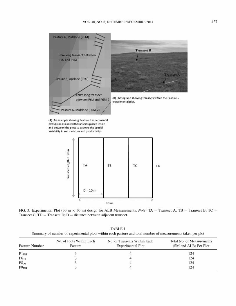
estimation of ALB. In general, vegetation clipping to estimateplant productivity is destructive and time consuming (for exam-ple, sorting live from dead biomass). Additionally, destructivesampling can be problematic for field studies conducted in con-served or managed areas where management objectives includeminimized environmental disturbance. Therefore, to developrelationships between ALB and imagery, field work was con-ducted combining limited destructive sampling with extensiveuse of field-based radiometry (also used in a parallel study; onlydetails directly relevant to this paper are reported here). Basedon visual survey of the pastures, experimental plots were set upin 2 grazed pastures (P633 and P870) and 2 ungrazed pastures(P1UG and P9UG) in the summer of 2008. To capture likely graz-ing patterns with respect to proximity to water, the experimentalplots were positioned between Horse Creek and Wetherall Creekto include upslope (U), midslope (M), and downslope (D) posi-tions. Three experimental plots, each 30 m x 30 m in size, wereplaced within the selected pastures (Figure 1 and Figure 3). Plotlocations were identified using a handheld Global PositioningSystem (GPS) with a horizontal accuracy of 2 m, and wereflagged with a pasture and plot number, using the labeling con-vention P9U, P9M and P9D (U = upslope, M = midslope, andD = downslope).

A CropScan1 MSR5 ground radiometer was used to takeNormalized Difference Vegetation Index (NDVI) measurements

1CropScan Inc., USA

every meter on each of 4, 30-m transects in each plot (Figure 3and Table 1).

Within a 30-m transect, ALB measurement was taken every1 m.

The radiometer was mounted 1.5 m above the ground and hadan instantaneous field of view of 28o, giving a spatial resolutionof approximately 0.75 m on the ground at nadir. All the radiome-ter readings were taken within 2 hours of local solar noon. Threereadings per point were taken and averaged to smooth out anyinstrument error. The rationale behind the distance between 2samples was to capture the local variability of ALB (details ofestimation follow). Equally important, however, the experimen-tal plots were a reasonable size to be able to feasibly sample thepastures during the time frame of the study.

Depending on the objective and scale of the research, bothground-based radiometers and satellite imagery have beenwidely utilized within grassland research to estimate plant bio-physical parameters such as ALB (Davidson and Csillag 2001;Flombaum and Sala 2007). Typically, ALB is estimated by es-tablishing an empirical relationship between the destructivelymeasured biomass and the transformations of 2 or more re-motely sensed spectral bands. Davidson and Csillag (2001) ex-amined the relationship between numerous spectral vegetationindices and ALB in GNP, Saskatchewan, and found that fortheir purposes, all the vegetation indices produced similar re-sults. Flynn et al. (2008) concluded that the spatial variabilityof biomass in pastures and hayfields can be determined accu-rately using the NDVI measured from a ground-based sensor.Our CropScan measurements comprised reflectance in wave-lengths corresponding to Landsat Bands 1–5, meaning a num-ber of vegetation indices were available. Preliminary analysisshowing high correlation between the NDVI and the EnhancedVegetation Index (EVI) (R2 = 0.94, p < 0.05), plus Davidsonand Csillag’s (2001) results, prompted a decision to consideronly NDVI for further analysis.

Twelve destructive biomass samples were collected for ra-diometer calibration purposes at random locations near theexperimental transects, followed by biomass clipping in 50× 10 cm rectangles. All aboveground vegetation was clipped

VOL. 40, NO. 6, DECEMBER/DECEMBRE 2014 427

FIG. 3. Experimental Plot (30 m × 30 m) design for ALB Measurements. Note: TA = Transect A, TB = Transect B, TC =Transect C, TD = Transect D; D = distance between adjacent transect.

TABLE 1Summary of number of experimental plots within each pasture and total number of measurements taken per plot

Pasture NumberNo. of Plots Within Each

PastureNo. of Transects Within Each

Experimental PlotTotal No. of Measurements

(SM and ALB) Per Plot

P1UG 3 4 124P633 3 4 124P870 3 4 124P9UG 3 4 124

428 CANADIAN JOURNAL OF REMOTE SENSING/JOURNAL CANADIEN DE TELEDETECTION

FIG. 4. Calibration curve for converting field-measured NDVIto area biomass (g m−2).

using shears and was stored in sealed plastic bags. The vege-tation was transported back to the research station and sorted,dried, and weighed within 60 hrs (≤ 36 hours for sorting, fora related project, plus 24 hours oven-drying at 60◦C, or until aconstant weight was achieved). These data were combined withsimilar but more extensive field data (vegetation type: grass, se-laginella/lichen, forb/shrubs and juniper) collected by Davidsonet al. (2006) and Miles (2009) to derive the calibration of Equa-tion (1), used here (R2 = 0.61, p = 0.000, N = 130; Figure 4).

Biomass = (5.9803)e(5.873 ∗ Field−measuredNDVI) [1]

Satellite DataPrevious studies in semiarid regions found Landsat TM data

to be very well suited for estimating biomass and cover un-der different management practices, as well as appropriate formeasuring spatial heterogeneity in grasslands (Guo et al. 2000;Zhang et al. 2003). He et al. (2006) suggested that a pixel size of∼35 m would capture most of the spatial variation in biophysicalproperties of grasslands in this study area (i.e., GNP). Similarly,Davidson and Csillag (2001) determined that resolutions from10 m–50 m had potential for estimating C4 species coveragein the GNP area. Therefore, Landsat TM was selected for thisstudy because of its resolution (pixel size approximately 30 m)and availability. Despite better temporal resolution (8 days) thanLandsat (16 days), coarser imagery such as Moderate Resolu-tion Imaging Spectroradiometer (MODIS) (250 m and 500 mpixel size) and AVHRR (1.1 km pixel size) were not used, be-cause they would not have been able to detect important spatialpatterns below these scales.

The satellite data used in this study consisted of 5 Landsat(TM) scenes (Path/Row: 36/26 and 37/26, as shown in Table 2).Images covering the East Block, GNP, and Mankota commu-nity pasture were acquired from the United States GeologicSurvey (USGS) Earth Resource Observation and Science Center(EROS)2 using a maximum 10% cloud cover selection criterion.

2http://glovis.usgs.gov/

TABLE 2Landsat TM image acquisition information

Landsat Image Acquisition Date Path/Row

June 30, 2000 37/26June 27, 2007 36/26June 29, 2008 36/26June 23, 2009 37/26June 26, 2010 37/26

Image PreprocessingThe Fast Line-of-sight Atmospheric Analysis of Spectral

Hypercubes (FLAASH) algorithm based on MODTRAN 4,within ENVI image processing software3 was used for atmo-spheric correction on the Landsat scenes. This algorithm hasbeen tested and shown to be accurate by Mathew et al. (2003)and Davis (2006). The algorithm has the benefit of not requiringany ancillary data other than solar zenith angle and visibilityat the time of acquisition, which was acquired from the imagemetadata. From the standard MODTRAN model atmospheres,mid-latitude summer (MLS) model atmosphere was selectedfor atmospheric information (e.g., water vapor and surface airtemperature). Visibility over the GNP area for each date wasobtained from the Environment Canada (2010) website. TheFLAASH algorithm was then applied to all bands for all thescenes.

Identification of Grazed and Ungrazed Sites with VariableGrazing Intensity (GI)

Only the portions of each image that were over the studyarea were analyzed. Vector files that delineated the East Block(GNP) and Mankota community pastures were used to clip theregion of interest (ROI) from the Landsat scenes to ensure thatother land uses, such as cultivated agriculture, did not impactthe results.

Sampling Design for Satellite-Based Data AnalysesEach experimental pasture was analyzed to determine the

ALB variability within the pastures. Additionally, transect sam-pling design was used to see if slope position (upslope anddownslope) had any impact on the ALB heterogeneity. Transectlength was dependent on the size of the upslope and downslopearea within each experimental pasture of the East Block andMankota community pasture.

3ENVI, 2008; http://www.exelisvis.com/ProductsServices/ENVIProducts.aspx

VOL. 40, NO. 6, DECEMBER/DECEMBRE 2014 429

Weather DataPlant productivity is affected by various factors, including

weather (Knapp et al. 2002). To better understand the in-teraction between site-specific weather conditions and ALB,an AE50 HOBO Weather Station4 was installed in P9UG.From May 15 to August 21, 2008, it recorded precipitation,temperature, photosynthetically active radiation, relative hu-midity, wind direction, and speed. Mankota weather stationdata acquired from Environment Canada (2010) were alsoused to assess inter- and intraseasonal conditions affecting theALB.

DATA ANALYSIS AND METHODSData were checked for normal distribution using the

Kolmogorov–Smirnov test (p-value > 0.05), and were log-transformed where needed to satisfy assumptions of normalityand homogeneity of variance. Additionally, data were testedfor homoscedasticity using Levene’s test (Levene 1960) andBartlett’s test (Snedecor and Cochran 1989).

Mixed effect models—linear mixed effect models (LME)and generalized linear mixed effect models (GLMEs)5—wereused to separate the fixed effects (i.e., where all levels of aneffect are represented) of management (grazing treatment) andslope location from the random effects (i.e., where levels of aneffect are assumed random and not fully represented; in thisstudy, this included pasture as a random sampling variable) asin Bell and Grunwald (2004) and Mandle and Ticktin (2012).The year was treated as a fixed effect because treatment couldhave cumulative effects over time because cattle remove vegeta-tion every season, and the amount and distribution of remainingvegetation in year n + 1 depends on the amount of vegetationremoved in year n. The rationale for using mixed effects modelswas their ability to analyze repeated measures data, allowing forsequential sampling from a single plot over multiple dates, andthe use of both categorical and continuous effects (variables)simultaneously (Piepho et al. 2003; McCulley et al. 2005). Fi-nally, including random effects in statistical analyses allows usto make inferences beyond the scope of this study, comparedto conclusions from fixed effects treatments that can be ap-plied only to differences among those treatments addressed inthe study. The temporal data were analyzed using the repeated-measures ANOVA procedure of the SPSS general linear modelto estimate the overall significance of treatment effects. Whengrazing treatment by year interaction or year effects were sig-nificant (p ≤ 0.05), the Tukey–Kramer Honestly SignificantDifference (Tukey’s HSD) multiple comparisons test (Sasakiet al. 2009) and the Bonferroni corrected test were used to de-termine which treatment-year combinations and which yearsdiffered.

4Onset Computer Corporation, 2007, www.onsetcomp.com/5SPSS version 20.0, IBM Corporation, New York, USA

Geostatistical Analysis Using SemivariogramsGeostatistics handles data sampled in space, allowing the

exploration of variability with respect to distance. Most para-metric statistics are inadequate to analyze spatially dependentvariables because the assumption is that all the measured ob-servations are independent (Cambardella et al. 1994). However,in geostatistics it is assumed that there is spatial autocorrelation(spatial dependence) in the variables, which can be measuredand analyzed. Therefore, semivariogram analysis was used inthis study to detect the range and spatiotemporal variability inALB under ungrazed and grazed conditions (e.g., Flynn et al.2008; Lin et al. 2010). Spatiotemporal changes in satellite-basedALB estimates were quantified using semivariance analyses of5 Landsat scenes taken June 2000 and June 2007 through 2010.Once experimental semivariograms were calculated, a modelwas fitted to the semivariogram to assess spatial correlation.Exponential models were used, as this form was found to pro-vide the best fit, with minimum error, and low residual sumsof squares (RSS) value (0.00004 to 0.0094). The exponentialmodel is similar to the spherical model in that it approachesthe sill gradually, but different in the rate at which the sill isapproached and in the fact that the model and the sill neveractually converge. The equation used for this model is:

γ (h) = C0 + C[1 − exp(−h/A0)], [2]

where γ (h) = semivariance for interval distance class h, h = laginterval, C0 = nugget variance ≥ 0, C = structural variance ≥C0, and A0 = range parameter (Robertson 2008).

Once a variogram model was fit to the data, the parameters,range (A0), sill (C0 + C, and nugget (C0) were derived.

Measures of HeterogeneityOnce semivariogram models were derived, 4 derivatives were

also calculated to further characterize heterogeneity: correlationratio (CR), spatial dependence ratio (SDR; or nugget%), magni-tude of spatial heterogeneity (MSH), and relative heterogeneity(SH%).

Correlation ratio is the proportion of the nugget effect valuesto the sill, where values near zero indicate continuity in spatialdependence (Vieira and Gonzalez 2003). It was calculated as:

CorrelationRatio = NuggetEffect

NuggetEffect + Sill[3]

Spatial dependence ratio (SDR) or Nugget% was calculatedbased on Cambardella et al. 1994.

SDR =(

NuggetVariance

TotalVariance

)∗ 100 [4]

This ratio was used to define the spatial dependency classesfor soil moisture and ALB. If SDR was (a) ≤ 25%, the vari-able was considered strongly spatial dependent, (b) between25% and 75%, the variable was considered moderately spatially

430 CANADIAN JOURNAL OF REMOTE SENSING/JOURNAL CANADIEN DE TELEDETECTION

dependent, (c) > 75%, the variable was considered weakly spa-tially dependent (based on Cambardella et al. 1994).

MSH is measured as the proportion of total sample variationaccounted for by spatially structured variation (Lin et al. 2010).

MSH =(

C

Co + C

)[5]

Spatial variance (C) can be calculated as follows:

C = [Co + C] − Co [6]

Here, is the nugget variance representing random variation(i.e., homogeneity); Co + C is the sill representing maximum(or total) variation and is spatial variance.

MSH and SH have been widely used to estimate the mag-nitude of spatial dependence for different soil variables withina site (Robertson et al. 1993; Boerner et al. 1998; Lin et al.2010). Values for MSH range from 0 to 1, where a value of zeroindicates no spatially structured heterogeneity (i.e., samples atall separation distances are independent from each other) and avalue of 1 indicates a high amount of spatially structured het-erogeneity. Both MSH and spatial dependence are correlated;the higher the MSH, the stronger the spatial dependence.

The proportion of the autocorrelated spatial heterogeneity inthe total variation is represented by SH%, which is calculatedfrom the nugget variance and sill (Li and Reynolds 1995):

SH% =(

SillVariance − NuggetVariance

SillVariance

)∗ 100 [7]

Therefore, autocorrelated variation (heterogeneity) can becalculated by subtracting the random variation (nugget) fromthe total variation (sill).

Similar to MSH, SH% is also positively correlated with thespatial dependence. Similar to the Western et al. (2004) study,correlations were also calculated between the averaged SM andsemivariogram variables such as sill, range, and MSH; as wellas averaged ALB and semivariogram variables.

CorrelogramsCorrelograms were also calculated to provide the evidence

for the size of the zone of influence and the type of spatialpattern (clustered, dispersed, or random) of the variable understudy. The number of observations per distance class and themaximum extent for interpretation of a correlogram varied withthe spatial configuration of the 2 sampling designs: transectand grid. The maximum extent of interpretation ranged from1,200 m for transect, and 1,200 m and 2,400 m for grid design.

RESULTS

Local Weather VariabilityBecause weather variability has implications for plant

growth, Mankota weather station data (Environment Canada

FIG. 5. Total monthly rainfall (mm) and average monthly airtemperatures (◦C) for growing season in year 2000, 2007, 2008,2009, and 2010 for the study area.∗Because 2007 precipitation and average air temperature datafor May was available only from day 19 onwards, in this graphonly days 19 to 31 are presented.

2010) were analyzed to assess inter- and intraseasonal con-ditions. Total monthly rainfall and average monthly air tem-peratures for the 2000 and 2007 to 2010 growing seasons arepresented in Figure 5. More rainfall was recorded during the2010 growing season (292.04 mm) compared to all other years(244.80 mm, 174.60 mm, 121.80 mm, and 147.38 mm). Juneusually received the most rainfall, except in 2009. Timing andamount of rainfall received were also highly variable betweenyears and events. Compared to the other years, 2007 showedhigher average air temperatures during June and July.

Effect of Different Grazing Intensities on ALBSpatiotemporal Heterogeneity

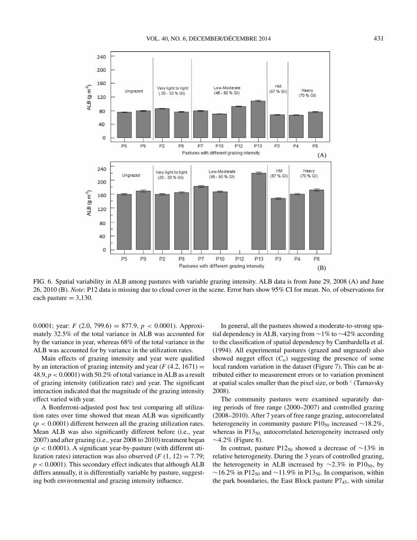
There was considerable variability in ALB between low mod-erate (LM), high moderate (HM), and heavy (H) grazing inten-sities after 2 years of grazing (Figure 6). Overall, LM had thehighest ALB in both 2008 and 2010.

Both grazing intensity (utilization rate) and year significantlyaffected the ALB (grazing intensity: F (2.2, 894) = 115.4, p <

VOL. 40, NO. 6, DECEMBER/DECEMBRE 2014 431

FIG. 6. Spatial variability in ALB among pastures with variable grazing intensity. ALB data is from June 29, 2008 (A) and June26, 2010 (B). Note: P12 data is missing due to cloud cover in the scene. Error bars show 95% CI for mean. No. of observations foreach pasture = 3,130.

0.0001; year: F (2.0, 799.6) = 877.9, p < 0.0001). Approxi-mately 32.5% of the total variance in ALB was accounted forby the variance in year, whereas 68% of the total variance in theALB was accounted for by variance in the utilization rates.

Main effects of grazing intensity and year were qualifiedby an interaction of grazing intensity and year (F (4.2, 1671) =48.9, p < 0.0001) with 50.2% of total variance in ALB as a resultof grazing intensity (utilization rate) and year. The significantinteraction indicated that the magnitude of the grazing intensityeffect varied with year.

A Bonferroni-adjusted post hoc test comparing all utiliza-tion rates over time showed that mean ALB was significantly(p < 0.0001) different between all the grazing utilization rates.Mean ALB was also significantly different before (i.e., year2007) and after grazing (i.e., year 2008 to 2010) treatment began(p < 0.0001). A significant year-by-pasture (with different uti-lization rates) interaction was also observed (F (1, 12) = 7.79;p < 0.0001). This secondary effect indicates that although ALBdiffers annually, it is differentially variable by pasture, suggest-ing both environmental and grazing intensity influence.

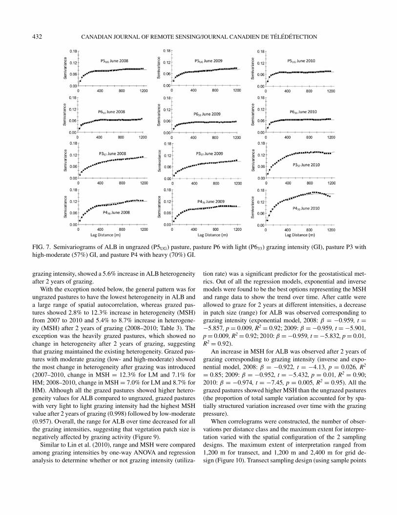
In general, all the pastures showed a moderate-to-strong spa-tial dependency in ALB, varying from ∼1% to ∼42% accordingto the classification of spatial dependency by Cambardella et al.(1994). All experimental pastures (grazed and ungrazed) alsoshowed nugget effect (Co) suggesting the presence of somelocal random variation in the dataset (Figure 7). This can be at-tributed either to measurement errors or to variation prominentat spatial scales smaller than the pixel size, or both ◦ (Tarnavsky2008).

The community pastures were examined separately dur-ing periods of free range (2000–2007) and controlled grazing(2008–2010). After 7 years of free range grazing, autocorrelatedheterogeneity in community pasture P1050 increased ∼18.2%,whereas in P1350, autocorrelated heterogeneity increased only∼4.2% (Figure 8).

In contrast, pasture P1250 showed a decrease of ∼13% inrelative heterogeneity. During the 3 years of controlled grazing,the heterogeneity in ALB increased by ∼2.3% in P1050, by∼16.2% in P1250 and ∼11.9% in P1350. In comparison, withinthe park boundaries, the East Block pasture P745, with similar

432 CANADIAN JOURNAL OF REMOTE SENSING/JOURNAL CANADIEN DE TELEDETECTION

FIG. 7. Semivariograms of ALB in ungrazed (P5UG) pasture, pasture P6 with light (P633) grazing intensity (GI), pasture P3 withhigh-moderate (57%) GI, and pasture P4 with heavy (70%) GI.

grazing intensity, showed a 5.6% increase in ALB heterogeneityafter 2 years of grazing.

With the exception noted below, the general pattern was forungrazed pastures to have the lowest heterogeneity in ALB anda large range of spatial autocorrelation, whereas grazed pas-tures showed 2.8% to 12.3% increase in heterogeneity (MSH)from 2007 to 2010 and 5.4% to 8.7% increase in heterogene-ity (MSH) after 2 years of grazing (2008–2010; Table 3). Theexception was the heavily grazed pastures, which showed nochange in heterogeneity after 2 years of grazing, suggestingthat grazing maintained the existing heterogeneity. Grazed pas-tures with moderate grazing (low- and high-moderate) showedthe most change in heterogeneity after grazing was introduced(2007–2010, change in MSH = 12.3% for LM and 7.1% forHM; 2008–2010, change in MSH = 7.0% for LM and 8.7% forHM). Although all the grazed pastures showed higher hetero-geneity values for ALB compared to ungrazed, grazed pastureswith very light to light grazing intensity had the highest MSHvalue after 2 years of grazing (0.998) followed by low-moderate(0.957). Overall, the range for ALB over time decreased for allthe grazing intensities, suggesting that vegetation patch size isnegatively affected by grazing activity (Figure 9).

Similar to Lin et al. (2010), range and MSH were comparedamong grazing intensities by one-way ANOVA and regressionanalysis to determine whether or not grazing intensity (utiliza-

tion rate) was a significant predictor for the geostatistical met-rics. Out of all the regression models, exponential and inversemodels were found to be the best options representing the MSHand range data to show the trend over time. After cattle wereallowed to graze for 2 years at different intensities, a decreasein patch size (range) for ALB was observed corresponding tograzing intensity (exponential model, 2008: β = −0.959, t =−5.857, p = 0.009, R2 = 0.92; 2009: β = −0.959, t = −5.901,p = 0.009, R2 = 0.92; 2010: β = −0.959, t = −5.832, p = 0.01,R2 = 0.92).

An increase in MSH for ALB was observed after 2 years ofgrazing corresponding to grazing intensity (inverse and expo-nential model, 2008: β = −0.922, t = −4.13, p = 0.026, R2

= 0.85; 2009: β = −0.952, t = −5.432, p = 0.01, R2 = 0.90;2010: β = −0.974, t = −7.45, p = 0.005, R2 = 0.95). All thegrazed pastures showed higher MSH than the ungrazed pastures(the proportion of total sample variation accounted for by spa-tially structured variation increased over time with the grazingpressure).

When correlograms were constructed, the number of obser-vations per distance class and the maximum extent for interpre-tation varied with the spatial configuration of the 2 samplingdesigns. The maximum extent of interpretation ranged from1,200 m for transect, and 1,200 m and 2,400 m for grid de-sign (Figure 10). Transect sampling design (using sample points

VOL. 40, NO. 6, DECEMBER/DECEMBRE 2014 433

FIG. 8. Semivariograms of ALB in low-moderate grazing intensity (50%) pastures 10 (P1050) and 13 (P1350) located in Mankotacommunity pasture. Note: Semivariograms for years 2000 and 2007 represent pastures with free range grazing, whereas semivari-ograms for years 2008 to 2010 represent pastures with controlled low-moderate grazing.

along transect placed within a pasture) exhibited a wavelike pat-tern within the experimental pastures. For example, in the P220

correlogram, the first change of sign from positive to negativevalue occurred around 60 m, which corresponded to the spatialrange of the patches.

The correlogram showed some repetitive patterns of patches;however, both the patch size and the distances among the patches

were quite variable. Similarly, other experimental pastures suchas P357, P870 (Figure 10), and P1350 also showed patchy spa-tial pattern with variable patch size and distance among thepatches. In comparison, P220’s spatial correlogram based on thegrid sampling design (1,200 m extent) showed a gradient spa-tial pattern with significant positive values at short distancesto negative values at large distances. However, it leveled at

434 CANADIAN JOURNAL OF REMOTE SENSING/JOURNAL CANADIEN DE TELEDETECTION

TABLE 3Summarized sill, range, and MSH results for different grazing intensities for years 2007, 2008, and 2010

Year GI Sill (C + Co) Range (m) MSH (C / [C + Co])

2007 (No grazing) UG 0.180 1,348 0.690VLLBG 0.143 324 0.970LMBG 0.124 315.2 0.834HMBG 0.212 257 0.894HBG 0.239 172 0.938

2008 (Start of grazing) UG 0.122 1,294 0.658VLLAG 0.075 249 0.944LMAG 0.075 293 0.887HMAG 0.107 324 0.838HAG 0.128 188 0.942

2010 (after 2 years of grazing) UG 0.099 1,353 0.652VLLAG 0.063 180 0.998LMAG 0.095 236 0.957HMAG 0.133 212 0.925HAG 0.153 180 0.941

Note: GI = grazing intensity; BG = before grazing; AG = after grazing; UG = ungrazed; VLL = very light to light grazing (20%–33% GI);LM = low-moderate grazing (45%–50% GI); HM = high-moderate grazing (57% GI); and H = heavy grazing (70% GI); MSH = magnitudeof spatial heterogeneity.

around zero, indicating absence or nondetection of spatial pat-terns at distances > 220 m. Similarly, pastures P357, P870, andP1350 showed positive values at short distances with significantspatial autocorrelation. P357 and P870 also showed alternationof values from positive to negative, thus indicating patchiness.Correlations for P1350 oscillated along the zero value suggest-ing absence of any significant spatial autocorrelation at largedistances. The spatial range (zone of influence, patch size) forpasture P1350 was around 360 m, a distance at which the signof the values changed from positive to negative.

Overall, correlograms based on either of 2 sampling designswere globally significant, indicating that the overall spatial pat-tern of ALB is not random, but it is likely that there are spatialpatterns existing at smaller distances than the distances between

sampling pixels, which could not be detected by the grid sam-pling design (Wiens 1989). Smooth curves displayed by thegrid sampling design compared to transect design are due toaveraging over several directions. The patterns are clearer forgrid sampling design when correlograms were calculated for2,400 m extent.

A significant effect of grazing intensity on ALB was foundeven after controlling for the effect of slope position (F (4,943) = 12.74, p < 0.001; N = 953). Post hoc test (Tukey’sHSD) results indicated that mean ALB values were signifi-cantly different (p < 0.001) between the upslope and downs-lope locations for all the grazing intensities, where downs-lope areas showed higher mean ALB values than upslopeareas.

FIG. 9. Comparison of mean MSH and mean range of influence between different grazing intensities for no grazing (year 2007),at the start of the grazing (year 2008), after 1 year of grazing (year 2009), and after 2 years of grazing (year 2010).

VOL. 40, NO. 6, DECEMBER/DECEMBRE 2014 435

FIG. 10. Effect of grazing intensity and sampling design (Grid vs. Transect) on the ALB spatial pattern (Moran’s I): An exampleof VLL (P220), HM (P357), and heavy grazing (P870) is provided. (Lag distance = 1200 m for Transect and Grid; 2400 m forGrid only, lag class distance interval = 30 m). Note: P220 = pasture 2 with very light to light (20%) grazing intensity (GI); P357

= pasture 3 with high-moderate (57%) GI; P870 = pasture 8 with heavy (70%) GI. Solid squares indicate significant coefficientvalues at α = 0.05; open squares indicate nonsignificant coefficient values after progressive Bonferroni correction.

DISCUSSION

Spatial Heterogeneity in Grazed and Ungrazed PasturesAll the grazed pastures showed variability in ALB over the

years (Figure 6). Despite the variability in ALB, overall grazedpastures showed higher ALB than ungrazed pastures, whereALB was greatest in the moderately grazed pastures with 50%grazing intensity. The findings were consistent with Holechecket al. (2006) and Jamiyansharav et al. (2011), which also showedhigher biomass production in the moderately grazed pasturesthan in the ungrazed sites.

NDVI and, therefore, the estimated ALB (g m−2) values in-creased and decreased over the years within grazed and ungrazedpastures, which is common in semiarid grasslands (Milchunaset al. 1994). This is because temporal (seasonal and interannual)variability in plant processes is largely a function of changes insoil temperature and moisture over time (Epstein et al. 2002;Knapp et al. 2002). Due to satellite data limitations and im-agery quality at the desired scale, it was not possible to separatethe effect of interannual variation on the mean ALB valuesin the grazed pastures. This is because desired image quality(< 10% cloud cover and shadows) for the study area limitedthe scene acquisition to single dates in 1 or 2 months of thegrowing season, for example, June 29, 2008, June 23, 2009, and

June 26, 2010. This resulted in insufficient data samples to runthe correlation analysis to determine the impact of both rainfalland grazing intensity on ALB variability. Therefore, to differ-entiate rainfall-induced fluctuations from changes in vegetationdynamics caused by different grazing intensities, monitoringmust include seasonal data and/or interannual data for long pe-riods in order to have adequate sample size.

The study area showed variation in the weather conditionsover a 4-year study period. Both timing and amount of rainfallreceived were highly variable between the years and events(Figure 5). A study conducted by Fay et al. (2000), for a mesicgrassland ecosystem located in northeastern Kansas, identifiedrainfall interval as the primary influence on the soil and plantresponses, with increased intervals causing reduction in totalaboveground net primary productivity (ANPP) and floweringduration. This is because increased intervals between rainfallevents can create soil water deficits, thus affecting the availablewater for plant growth.

A significant linear correlation was found between theamount of biomass available for grazing and grazing intensity(R2 = 0.862, p < 0.0001), where, in general, ALB increasedwith grazing intensity. Wallace and Crosthwaite (2005) alsoreported a significant linear correlation between biomass andgrazing intensity (R2 = 0.365, p < 0.0001). However, ALB for

436 CANADIAN JOURNAL OF REMOTE SENSING/JOURNAL CANADIEN DE TELEDETECTION

57% and 70% grazing intensity was lower compared to VLLand LM grazing intensities.

The semivariogram analysis showed higher spatial hetero-geneity in ALB for grazed pastures with variable utilizationrates than ungrazed pastures (Table 3). A study by Johnsonet al. (2011) on grazing intensity effects on grassland birds alsoshowed increased heterogeneity over time with increase in graz-ing intensity. In this study, heavily grazed pastures showed thehighest ALB heterogeneity in 2007 (no grazing year) comparedto other pastures. However, after the introduction of grazing inyear 2008, higher heterogeneity in ALB over time was observedin VLL and LM pastures than heavily grazed pastures, indicat-ing a quadratic effect (Figure 9). Similarly, Lin et al. (2010) re-ported a quadratic relationship between the ALB heterogeneityand stocking rates. Overall, grazed pastures showed increasedheterogeneity after 2 years of grazing with high-moderate graz-ing, showing the highest change in heterogeneity under low-moderate grazing intensity. An exception was heavily grazedpastures, which showed no change in heterogeneity after 2 yearsof grazing, suggesting that grazing maintained the heterogeneityover the years. It is likely that forage availability remained highenough, even under the highest utilization rate, that cattle did nothave to utilize previously ungrazed patches during the grazingperiod, which most likely would have homogenized the vege-tation structure to some degree. Similar studies of the effectsof grazing intensity on spatial heterogeneity of vegetation havedocumented changes (increase or decrease) in spatial hetero-geneity over time, where study results are likely affected by thevegetation utilization level, response variable, and spatial scaleevaluated (Townsend and Fuhlendorf 2010). Because the man-agement goals for the GNP include increasing species hetero-geneity as essential to maintaining and sustaining biodiversitywithin the GNP, 70% grazing intensity may be too high. How-ever, other studies document the association of some rare nativeplants (example, blowout penstemon, Penstemon haydenii) andanimals (such as the black-footed ferret and mountain plover)with heavily grazed areas (Klute et al. 1997; Stubbendieck et al.1997). Therefore, if economically possible, a range of grazingintensities (low-moderate-heavy) will be more suitable for theGNP in providing habitats for a greater suite of species prefer-ring variable vegetation cover than incorporating limited rangesof grazing intensities (low and moderate).

Based on personal observation during the field work con-ducted in summer 2008, soil characteristics, vegetation type(grass, shrubs, forbs, and other) within the lowland, upland,and riparian areas of each pasture, and cover (sparse, dense,bare, or mixed) was highly variable among the experimentalpastures. This is likely the cause of variation in addition to lo-cal weather variation within the ungrazed pastures (Vallentine2001; Harrison et al. 2003). In comparison, grazing activity is aninfluencing factor for the variability in ALB in the grazed pas-tures. For example, compaction due to grazers can alter the soilstructure, which may change the soil aeration and moisture re-tention capacity, affecting the plant available water (Jacobs et al.

2004). Any change in plant available water will further impactthe plant growth as well as plant productivity, thus contributingto more variability between the grazed and ungrazed pastures.In short, grazing disturbance can help create and maintain theheterogeneity in ALB, which is crucial for the successful coex-istence of many grassland species (Fuhlendorf and Engle 2004;Vermeire et al. 2004).

Effects of Grazing Intensity and Slope Location on ALBGrazing intensity (utilization rates) and year significantly in-

fluenced the spatial variability in ALB (p < 0.0001). The meanALB values were also significantly different among the graz-ing intensities (p < 0.05). Overall, the reduction of ALB byintensive grazing (high-moderate to heavy) also led to the de-cline of range for ALB, suggesting that vegetation patch sizedecreased with grazing pressure. This supports a view of grazingas a characteristically patchy process (Adler et al. 2001), wherepatchiness could be due to plant defoliation, trampling, and ex-cretion during the grazing period (Damhoureyeh and Hartnett1997). For example, grazers’ excretory products are nutrientrich, which creates patches with elevated nutrients readily avail-able for plants. These nutrient-rich patches generally have al-tered plant species composition (Steinauer and Collins 2001).Also, some studies show that grazers often “patch graze” bypreferentially grazing some areas repeatedly while leaving otherareas ungrazed until forage availability is low (Coghenour 1991;Cid and Brizuela 1998). As a result of this preferential grazing,patchiness is either maintained or enhanced in time.

In addition, field pictures from summer 2008 in the EastBlock of the GNP showed a high amount of variability in thetype of vegetation within all the experimental pastures. For ex-ample, P870 showed presence of poisonous grass death camas(Zigadenus venenosus), which is avoided by the grazers. Thismay have also contributed to patchy patterns within the ex-perimental pasture. Additionally, vegetation patches with cowpatties and urine are generally avoided by the cattle in the sameyear (Steinauer and Collins 2001), which could have also addedto patchiness. Such patchy grazing tends to enhance biodiversity(Fuhlendorf and Engle 2004; Truett et al. 2001).

Cattle selectivity based on plant palatability and nutritivequality is likely one of the contributing factors for the patchyvegetation patterns. Generally, the nutritive quality of foragedeclines as the growing season progresses, which affects thecattle foraging decisions. This is because cool-season grasses(C3) have higher nutritive quality early in the season compared towarm-season grasses (C4) that grow later in the season (Adamset al. 1996). Additionally, variation in grazing intensity withlight grazing in some areas and heavy grazing in others alsoresults in a mosaic of vegetation types, thereby influencing notonly the plant community but diversity in animals and insectsas well (Hartnett et al. 1996; Knapp et al. 1999).

There was a significant effect of grazing intensity on ALBeven after controlling for the effect of slope position, and mean

VOL. 40, NO. 6, DECEMBER/DECEMBRE 2014 437

ALB values were significantly higher downslope. Plant com-munity composition is notably different between the upslopeand downslope areas, which may have led to some of the ob-served structural differences. Artificial water supplies and saltcubes were provided in uplands to encourage forage utilizationin these areas and to reduce cattle damage to riparian areas. Thisalso could have influenced the grazing patterns in the pastures,because water availability is an important factor in cattle forag-ing decisions (Briske et al. 2008). Studies such as Adler et al.(2001), Vallentine (2001), and Bradley and O’Sullivan (2011)concluded that factors such as slope, quality or desirability offorage, and distance to water influence the grazing distribution.

Spatial Patterns of ALB over TimeTwo sampling designs, grid and transect, were used to deter-

mine the spatial patterns in ALB with specific focus on smooth-ness of the correlogram. In our study, both designs were ableto detect the spatial patterns in ALB. However, a grid designprovided smoother correlograms as a result of more numbersof pairs per distance class than transect sampling design for thesame maximum distance.

Although coefficient of variance (CV; the standard deviationof a variable divided by its mean) measurements can provide anindication of the magnitude of variance, geostatistical analysisis needed to quantify different aspects of the spatial hetero-geneity, including the degree and range of autocorrelation (Liand Reynolds 1995). All the spatial correlograms showed thestrongest value of spatial autocorrelation within the first distanceclass and corresponded to the spatial range of the patches. For aseparation distance > 440 m and < 1,200 m, spatial autocorre-lation of ALB was generally neutral to slightly negative. Spatialautocorrelation of ALB in high-moderate and heavily grazedpastures was consistently close to zero at intermediate separa-tion distances, indicating some random variation. The lack ofspatial structure at intermediate distances might be indicative ofrandom arrangement of patches created as a result of grazingdisturbance (Cid and Brizuela 1998).

The spatial correlograms for the grazed experimental pas-tures based on transect sampling design exhibited a wavelikepattern compared to correlograms based on grid sampling designat the same maximum distance (1,200 m). The patchy patternobserved in both sampling designs is most likely caused by se-lective grazing by cattle, trampling, and waste deposition, whichprovide sites for plant germination as a result of high nutrientavailability (Sternberg et al. 2000). Overall, the correlogramsfrom both sampling designs showed some repetitive pattern ofpatches; however, both the patch size and the distances amongthe patches were quite variable.

CONCLUSIONSThe results from this study contribute to a developing body of

literature that suggests that the effects of livestock grazing on thespatial heterogeneity of vegetation is variable depending on the

grazing intensity, response variable, and spatial scale evaluated.Overall, observations show that low-to-moderate grazing inten-sity increases ALB heterogeneity over time, whereas no changein ALB heterogeneity over time was observed for heavy grazingintensity. As expected, all grazing intensities caused decreasein semivariogram range (patch size) over time, confirming thatgrazing is a patchy process. This study demonstrates that cattlegrazing with variable intensity both maintained and changed thespatial patterns of ALB in the studied mixed-grassland ecosys-tem because of the selective nature of the cattle. This informa-tion can be used in the development of effective grazing systemdesigns to maintain heterogeneity and restore biodiversity ingrassland ecosystems, which is one of the main goals of ParksCanada. Furthermore, to achieve production and conservationobjectives, many federal, provincial/state, and local organiza-tions within North America implement grazing practices forwhich one needs to consider heterogeneity as well as evaluatethe ecosystem responses to grazing intensities at spatial extents(pasture size 300 ha or larger) relevant for range managers.

We identify several future directions of research that couldfurther develop or refine these conclusions. First, we recom-mend that future studies should assess the impact of distancefrom watering points on the vegetation spatial patterns underdifferent grazing intensities. This will help with better under-standing of the impact of grazing intensity on overall hetero-geneity. Questions about weather variability and its impact onproduction are also important for looking at temporal variabilityof effects of grazing intensity on ALB heterogeneity. Becausegrasslands have developed under the influence of frequent andextensive fires and intensive grazing, both these disturbances arerequired for proper maintenance of grasslands (Coupland 1991;Hartnett et al. 1996; Fuhlendorf and Engle 2004; Vermeire et al.2004). Future grazing studies should incorporate the interac-tions of these disturbances on the ALB heterogeneity. Patchburning within a pasture is suggested as this will allow cattle toaccess both burned and unburned vegetation during subsequentgrowing seasons.

REFERENCESAdams, D. C., Clark, R. T., Klopfenstein, T. J., and Volesky, J. D. 1996.

“Matching the cow with the forage resources.” Rangelands, Vol. 18:pp. 57–62.

Adler, P. B., Raff, D. A., and Lauenroth, W. 2001. “The effect of grazingon the spatial heterogeneity of vegetation.” Oecologia, Vol. 128(No. 4): pp. 465–479.

Bai, Y. G., Abouguendia, Z., and Redmann, R. E. 2001. “Relationshipbetween plant species diversity and grassland condition.” Journal ofRange Management, Vol. 54(No. 2): pp. 177–183.

Bell, M. L., and Grunwald, G. K. 2004. “Mixed models for the analysisof replicated spatial point patterns.” Biostatistics, Vol. 5(No. 4): pp.633–648.

Boerner, R. E. J., Scherzer, A. J., and Brinkman, J. A. 1998. “Spatialpatterns of inorganic N, P availability, and organic C in relation tosoil disturbance: a chronosequence analysis.” Applied Soil Ecology,Vol. 7: pp. 159–177.

438 CANADIAN JOURNAL OF REMOTE SENSING/JOURNAL CANADIEN DE TELEDETECTION

Bradley, B. A., and O’Sullivan, M. T. 2011. “Assessing the short–termimpacts of changing grazing regime at the landscape scale with re-mote sensing.” International Journal of Remote Sensing, Vol. 32(No.20): pp. 5797–5813.

Briske, D. D., Derner, J. D., Brown, J. R., Fuhlendorf, S. D., Teague, W.R., Havstad, K. M., Gillen, R. L., Ash, A. J., and Willms, W. D. 2008.“Rotational grazing on rangelands: reconciliation of perception andexperimental evidence.” Rangeland Ecology and Management, Vol.61: 3–17.

Cambardella, C. A., Moorman, T. B., Novak, J. M., Parkin, T. B.,Karlen, D. L., Turco, R. F., and Konopka, A. E. 1994. “Field scalevariability of soil properties in Central Iowa soils.” Soil ScienceSociety of America Journal, Vol. 58(No. 5): pp. 1501–1511.

Cid, M. S., and Brizuela, M. A. 1998. “Heterogeneity in tall fescuepastures created and sustained by cattle grazing.” Journal of RangeManagement, Vol. 51(No. 6): pp. 644–649.

Coghenour, M. B. 1991. “Spatial components of plant–herbivoreinteractions in pastoral, ranching, and native ungulate ecosys-tems.” Journal of Range Management, Vol. 44(No. 6): pp.530–542.

Collins, S. L., Knapp, A. K., Briggs, J. M., Blair, J. M., and Steinauer,E. M. 1998. “Modulation of diversity by grazing and mowing innative tall grass prairie.” Science, Vol. 280: pp. 745–747.

Coupland, R. T. 1991. “Mixed prairie.” In Natural Grasslands: Intro-duction and Western Hemisphere, pp. 151–182. Ecosystems of theWorld, Vol. 8A. Amsterdam, The Netherlands: Elsevier.

Damhoureyeh, S. A., and Harnett, D. C. 1997. “Effects of bison and cat-tle on growth, reproduction, and abundances of five tallgrass prairieforbs.” American Journal of Botany, Vol. 84(No. 12): pp. 1719–1728.

Davidson, A., and Csillag, F. 2001. “The influence of vegetation indexand spatial resolution on a two-date remote sensing derived relationto C4 species coverage.” Remote Sensing of Environment, Vol. 75(No.1): pp. 138–151.

Davidson, A., Wang, S., and Wilhurmst, J. 2006. “Remote sensingof grassland–shrubland vegetation water content in the shortwavedomain.” International Journal of Applied Earth Observation andGeoinformation, Vol. 8(No. 4): pp. 225–236.

Davis, P. A. 2006. “Calibrated Landsat ETM+ non-thermal-band imagemosaics of Afghanistan.” U.S. Geological Survey Open-File Report2006-1345, 18 p. Washington, DC: U.S. Department of the Interior.

Derner, J. D., Lauenroth, W. K., Stapp, P., and Augustine, D. J. 2009.“Livestock as ecosystem engineers for grassland bird habitat in theWestern Great Plains of North America.” Rangeland Ecology andManagement, Vol. 62(No. 2): pp. 111–118.

Environment Canada. 2010. National Climate Data and InformationArchive. Accessed online December 3, 2010 at: http://www.climate.weatheroffice.gc.ca/climateData/canada e.html

Epstein, H. E., Burke, I. C., and Lauenroth, W. K. 2002. “Regionalpatterns of decomposition and primary production rates in the U.S.Great Plains.” Ecology, 83(No. 2): pp. 320–327.

Fay, P. A., Carlisle, J. D., Knapp, A. K., Blair, J. M., and Collins,S. L. 2000. “Altering rainfall timing and quantity in a mesic grass-land ecosystem: design and performance of rainfall manipulationshelters.” Ecosystems, 3(No. 3):pp. 308–319.

Flombaum, P., and Sala, O. E. 2007. “A non-destructive and rapidmethod to estimate biomass and aboveground net primary productionin arid environments.” Journal of Arid Environments, Vol. 69(No. 2):pp. 352–358.

Flynn, E. S., Dougherty, C. T., and Wendroth, O. 2008. “Assessmentof pasture biomass with the normalized difference vegetation indexfrom active ground–based sensors.” Agronomy Journal, Vol. 100:pp. 114–121.

Fortin, D., Fryxell, J. M., O’Brodovich, L., and Frandsen, D. 2003.“Foraging ecology of bison at the landscape and plant communitylevels: the applicability of energy maximization principles.” Oecolo-gia, Vol. 134: pp. 219–227.

Fuhlendorf, S. D., and Engle, D. M. 2004. “Application ofthe fire–grazing interaction to restore a shifting mosaic ontall grass prairie.” Journal of Applied Ecology, Vol. 41: pp.604–614.

Guo, X., Price, K. P., and Stiles, J. M. 2000. “Modeling biophysicalfactors for grasslands in Eastern Kansas using Landsat TM data.”Transactions of the Kansas Academy of Science, Vol. 103(No. 3/4):pp. 122–138.

Harrison, S., Inouye, B. D., and Safford, H. D. 2003. “Ecological het-erogeneity in the effects of grazing and fire on grassland diversity.”Conservation Biology, Vol. 17(No. 3): pp. 837–845.

Hart, R. H. 2001. “Plant biodiversity on shortgrass steppe after 55 yearsof zero, light, moderate, or heavy cattle grazing.” Plant Ecology, Vol.155(No. 1): pp. 111–118.

Hartnett, D. C., Hickman, K. R., and Walter, L. E.F. 1996. “Effects ofbison grazing, fire and topography on floristic diversity in tallgrassprairie.” Journal of Range Management, Vol. 49: pp. 413–420.

He, Y., Guo, X., Wilmhurst, J., and Si, B. C. 2006. “Studying mixedgrassland ecosystems II: optimal pixel size.” Canadian Journal ofRemote Sensing, Vol. 32(No. 2): pp. 108–115.

Hobbs, N. T. 1996. “Modification of ecosystems by ungulates.” Journalof Wildlife Management, Vol. 60(No. 4): pp. 695–713.

Holecheck, J. L., Baker, T. T., Boren, J. C., and Galt, D. 2006. “Grazingimpacts on rangeland vegetation: what we have learned livestockgrazing at light to moderate intensities can have positive impact onrangeland vegetation in arid to semiarid areas.” Rangelands, Vol.28(No. 1): pp. 7–13.

Jacobs, J. M., Mohanty, B. P., Hsu, E. C., and Miller, D. 2004.“SMEX02: field scale variability, time stability and similarity ofsoil moisture.” Remote Sensing of Environment, Vol. 92: 436–446.

Jamiyansharav, K., Ojima, D., Pielke, R. A., Parton, W., Morgan, J.,Beltran–Przekurat, A., LeCain, D., and Smith, D. 2011. “Seasonaland interannual variability in surface energy partitioning and veg-etation cover with grazing at shortgrass steppe.” Journal of AridEnvironments, Vol. 75(No. 4): pp. 360–370.

Johnson, T. N., Kennedy, P. L., DelCurto, T., and Taylor, R. V. 2011.“Bird community responses to cattle stocking rates in a Pacific North-west bunchgrass prairie.” Agriculture, Ecosystems and Environment,Vol. 144(No. 1):pp. 338–346.

Klute, D. S., Robel, R. J., and Kemp, K. E. 1997. “Will conversion ofConservation Reserve Program (CRP) lands to pasture be detrimentalfor grassland birds in Kansas?” American Midland Naturalist, Vol.137: pp. 206–212.

Knapp, A. K., Blair, J. M., Briggs, J. M., Collins, S. L., Hartnett, D.C., Johnson, L. C, and Towne, G. 1999. “The keystone role of bisonin North American tallgrass prairie.” Bioscience, Vol. 48(No. 1): pp.39–50.

Knapp, A. K., Fay, P. A., et al. 2002. “Rainfall variability, carboncycling, and plant species diversity in a Mesic Grassland.” Science,Vol. 298: pp. 2202–2205.

VOL. 40, NO. 6, DECEMBER/DECEMBRE 2014 439

Koper, N., Henderson, D., Wilmshurst, J. F., Fargey, P. J., and Sisson,R. A. 2008. “Design and analysis of rangeland experiments alongcontinuous gradients.” Rangeland Ecology and Management, Vol.61(No. 6): pp. 605–613.

Lauenroth, W. K., Burke, I. C., and Gutmann, M. R. 1999.“The structure and function of ecosystems in the central NorthAmerican grassland region.” Great Plains Research, Vol. 9: pp.223–259.

Levene, H. 1960. “Robust tests for equality of variances.” In Contribu-tions to Probability and Statistics, edited by I. Olkin. Palo Alto, CA:Stanford University Press, pp. 278–292.

Li, H., and Reynolds, J. F. 1995. “On definition and quantification ofheterogeneity.” Oikos, Vol. 73(No. 2): pp. 280–284.

Lin, Y., Hong, M., Han, G., Zhao, M., Bai, Y., and Chang, S. X. 2010.“Grazing intensity affected spatial patterns of vegetation and soil fer-tility in a desert steppe.” Agriculture, Ecosystems and Environment,Vol. 138(No. 3–4): pp. 282–292.

Mandle, L., and Ticktin, T. 2012. “Interactions among fire,grazing, harvest, and abiotic conditions shape palm demo-graphic responses to disturbance.” Journal of Ecology, doi:10.1111/j.1365–2745.2012.01982.x

Mathew, M. W., Adler-Golden, S. M., Berk, A., Felde, G., Anderson,G. P., Gorodetzky, D., Paswaters, S., and Shippert, M. 2003. “Atmo-spheric correction of spectral imagery: evaluation of the FLAASHalgorithm with AVIRIS data.” In Algorithms and Technologies forMultispectral, Hyperspectral and Ultraspectral Imagery IX, v. 5093,edited by S. S. Shen and P. E. Lewis, pp. 474–482. Orlando, FL: SPIE.

McCulley, R. L., Burke, I. C., Nelson, J. A., Lauenroth, W. K., Knapp,A. K., and Kelly, E. F. 2005. “Regional patterns in carbon cyclingacross the Great Plains of North America.” Ecosystems, Vol. 8,106–121.

Michalsky, S. J., and Ellis, R. A. 1994. Vegetation of Grass-lands National Park. Calgary, Canada: DA Westworth andAssociates.

Milchunas, D. G., Forwood, J. R., and Lauenroth, W. K. 1994. “Pro-ductivity of long-term grazing treatments in response to seasonalprecipitation.” Journal of Range Management, Vol. 47(No. 2): pp.133–139.

Miles, S. R. 2009. Relationships Between Net Primary Production, SoilMoisture and Topography in Semi-Arid Grassland Environments.Ottawa, Canada: Carleton University.

Parks Canada. 2002. Grasslands National Park of Canada: Manage-ment Plan, 79 pp.

Parks Canada 2005. [GNP Holdings as of 2002) and Roads] [map],1:2,300,000 approx. Grasslands National Park Map Files [ESRIShapefiles], DEM. Parks Canada, 2008, Using: ArcMap [GIS Soft-ware], Version 9.2, ESRI, 1999–2006.

Piepho, H. P., Buchse, A., and Emrich, K. 2003. “A hitchhiker’s guideto mixed models for randomized experiments.” Journal of Agronomyand Crop Science, Vol. 189: pp. 310–322.

Pinchak, W. F., Smith, M. A., Hart, R. H., and Waggoner, Jr., J. W.1991. “Beef cattle distribution patterns on foothills range.” Journalof Range Management, Vol. 44: pp. 267–275.

Robertson, G. P. 2008. GS+: Geostatistics for the Environmental Sci-ences. Plainwell, Michigan: Gamma Design Software.

Robertson, G. P., Crum, J. R., and Ellis, B. G. 1993. “The spatialvariability of soil resources following long–term disturbance.” Oe-cologia, 96(No. 4): pp. 451–456.

Sasaki, T., Okayasu, T., Ohkuro, T., Shirato, Y., Jamsran, U., andTakeuchi, K. 2009. “Rainfall variability may modify the ef-fects of long-term exclosure on vegetation on Mandalgobi, Mon-golia.” Journal of Arid Environments, Vol. 73 (No. 10): pp.949–954.

Saskatchewan Institute of Pedology 1992. Grasslands National ParkSoil Survey. Saskatoon, Canada: University of Saskatchewan.

Snedecor, G., Wand Cochran, W. G. 1989. Statistical Methods (8thed.). Ames, Iowa: Iowa State University Press.

Steinauer, E. M., and Collins, S. L. 2001. “Feedback loops in ecologicalhierarchies following urine deposition in tallgrass prairie.” Ecology,Vol. 82(No. 5): pp. 1319–1329.

Sternberg, M., Gutman, M., Perevolotshy, A., Ungar, E. D., and Kigel,J. 2000. “Vegetation response to grazing management in a Mediter-ranean herbaceous community: A functional group approach.” Jour-nal of Applied Ecology, 37: pp. 224–237.

Stubbendieck, J., Lamphere, J. A., and Fitzgerald, J. B. 1997. TheBlowout Penstemon, an Endangered Species (Brochure). Lincoln,NE: Nebraska Game and Parks Commission.

Tarnavsky, E., Garrigues, S., and Brown, M. E. 2008. “Multiscalegeostatistical analysis of AVHRR, SPT–VGT, and MODIS globalNDVI products.” Remote Sensing of Environment, Vol. 112: pp.535–549.

Townsend, D. E., and Fuhlendorf, S. D. 2010. “Evaluating rela-tionships between spatial heterogeneity and the biotic and abi-otic environments.” American Midland Naturalist, Vol. 163: pp.351–365.

Truett, J. C., Phillips, M., Kunkel, K., and Miller, R. 2001. “Managingbison to restore biodiversity.” Great Plains Research, Vol. 11(No.1): pp. 123–144.

Vallentine, J. F. 2001. Grazing Management. New York, NY: AcademicPress.

Vermeire, L. T., Mitchell, R. B., Fuhlendorf, S. D., and Gillen, R. L.2004. “Patch burning effects on grazing distribution.” Journal ofRange Management, Vol. 57: pp. 248–252.

Vieira, S. R., and Gonzalez, A. P. 2003. “Analysis of the spa-tial variability of crop yield and soil properties in smallagricultural plots.” Bragantia Campinas, Vol. 62(No. 1): pp.127–138.

Walter, D. W., Johan, F. D., Barry, W. A., and Harriet, E. D. 2002.“Response of the mixed prairie to protection from grazing.” Journalof Range Management, Vol. 55: pp. 210–216.

Wallace, L. L., and Crosthwaite, K. A. 2005. “The effect of fire spatialscale on bison grazing intensity.” Landscape Ecology, Vol. 20(No.3): pp. 337–349.

Weber, K. T., and Gokhale, B. S. 2011. “Effect of grazing on soil watercontent in semi-arid rangelands of southeast Idaho.” Journal of AridEnvironments, Vol. 75: pp. 464–470.

Western, A. W., Zhou, S.-K., Grayson, R. B., McMohan, T. A., Bloschl,G., and Wilson, D. J. 2004. “Spatial correlation of soil moisture insmall catchments and its relationships to dominant spatial hydro-logical processes.” Journal of Hydrology, Vol. 286(No. 1–4): pp.113–134.

Wiens, J. A. 1989. “Spatial scaling in ecology.” Functional Ecology,Vol. 3: pp. 385–397.

Zhang, C., Guo, X., Wilmshurst, J., and Fargey, P. 2003. “The role ofsatellite imagery resolution in the grassland heterogeneity measure-ment.” Environmental Informatics Archives, 1, 497–504.