graphing - home | casio · 2008-08-18 · 19990401 graphing sections 5-1 and 5-2 of this chapter...
TRANSCRIPT

19990401
GraphingSections 5-1 and 5-2 of this chapter provide basic informationyou need to know in order to draw a graph. The remainingsections describe more advanced graphing features and functions.
Select the icon in the Main Menu that suits the type of graph youwant to draw or the type of table you want to generate.• GRPH · TBL … General function graphing or number table generation• CONICS … Conic section graphing
(5-1-5 ~ 5-1-6, 5-11-17~5-11-21)• RUN · MAT … Manual graphing (5-6-1 ~ 5-6-4)• DYNA … Dynamic Graph (5-8-1 ~ 5-8-6)• RECUR … Recursion graphing or number table generation
(5-9-1 ~ 5-9-8)
5-1 Sample Graphs
5-2 Controlling What Appears on a Graph Screen
5-3 Drawing a Graph
5-4 Storing a Graph in Picture Memory5-5 Drawing Two Graphs on the Same Screen
5-6 Manual Graphing
5-7 Using Tables5-8 Dynamic Graphing
5-9 Graphing a Recursion Formula
5-10 Changing the Appearance of a Graph5-11 Function Analysis
Chapter
5
20011101
19990401
5-1-1Sample Graphs
5-1 Sample Graphs
kkkkk How to draw a simple graph (1)
DescriptionTo draw a graph, simply input the applicable function.
Set Up1. From the Main Menu, enter the GRPH • TBL Mode.
Execution2. Input the function you want to graph.
Here you would use the V-Window to specify the range and other parameters of thegraph. See 5-2-1.
3. Draw the graph.

19990401
5-1-2Sample Graphs
○ ○ ○ ○ ○
Example To graph y = 3x2
Procedure1m GRPH • TBL
2 dvxw
35(DRAW) (or w)
Result Screen

19990401
5-1-3Sample Graphs
kkkkk How to draw a simple graph (2)
DescriptionYou can store up to 20 functions in memory and then select the one you want for graphing.
Set Up1. From the Main Menu, enter the GRPH • TBL Mode.
Execution2. Specify the function type and input the function whose graph you want to draw.
You can use the GRPH • TBL Mode to draw a graph for the following types of expres-sions: rectangular coordinate expression, polar coordinate expression, parametricfunction, X = constant expression, inequality.
3(TYPE)b(Y =) ... rectangular coordinates
c(r =) ... polar coordinates
d(Param) ... parametric function
e(X = c) ... X = constant function
f(INEQUA)b(Y>)~e(Y<) ... inequality
g(CONV)b('Y=)~f('Y<) ... changes the function type
Repeat this step as many times as required to input all of the functions you want.
Next you should specify which of the functions among those that are stored in memoryyou want to graph (see 5-3-6). If you do not select specific functions here, the graphoperation will draw graphs of all the functions currently stored in memory.
3. Draw the graph.
20011101
19990401
5-1-4Sample Graphs
○ ○ ○ ○ ○
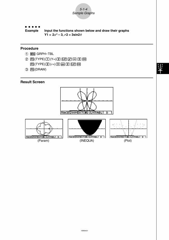
Example Input the functions shown below and draw their graphsY1 = 2x2 – 3, r2 = 3sin2θ
Procedure1m GRPH • TBL
23(TYPE)b(Y=)cvx-dw
3(TYPE)c(r=)dscvw
35(DRAW)
Result Screen
(Param) (INEQUA) (Plot)
19990401
5-1-5Sample Graphs
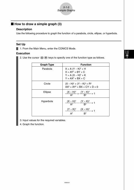
kkkkk How to draw a simple graph (3)
DescriptionUse the following procedure to graph the function of a parabola, circle, ellipse, or hyperbola.
Set Up1. From the Main Menu, enter the CONICS Mode.
Execution2. Use the cursor fc keys to specify one of the function type as follows.
3. Input values for the required variables.
4. Graph the function.
Graph Type Function
Parabola X = A (Y – K)2 + HX = AY2 + BY + CY = A (X – H)2 + KY = AX2 + BX + C
Circle (X – H)2 + (Y – K)2 = R2
AX2 + AY2 + BX + CY + D = 0
Ellipse (X – H)2 (Y – K)2
–––––––– + –––––––– = 1A2 B2
Hyperbola (X – H)2 (Y – K)2
–––––––– – –––––––– = 1A2 B2
(Y – K)2 (X – H)2
–––––––– – –––––––– = 1A2 B2
19990401
5-1-6Sample Graphs
○ ○ ○ ○ ○
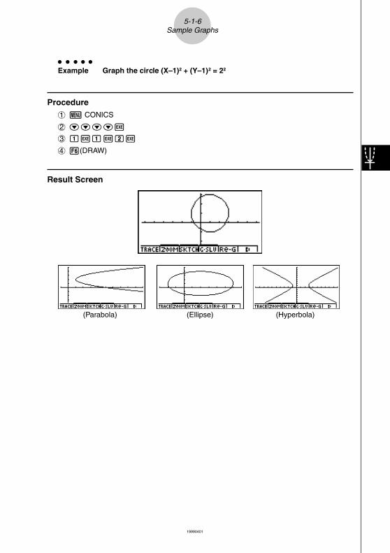
Example Graph the circle (X–1)2 + (Y–1)2 = 22
Procedure1m CONICS
2ccccw
3 bwbwcw
46(DRAW)
Result Screen
(Parabola) (Ellipse) (Hyperbola)
19990401
5-2 Controlling What Appears on a Graph Screen
kkkkk V-Window (View Window) Settings
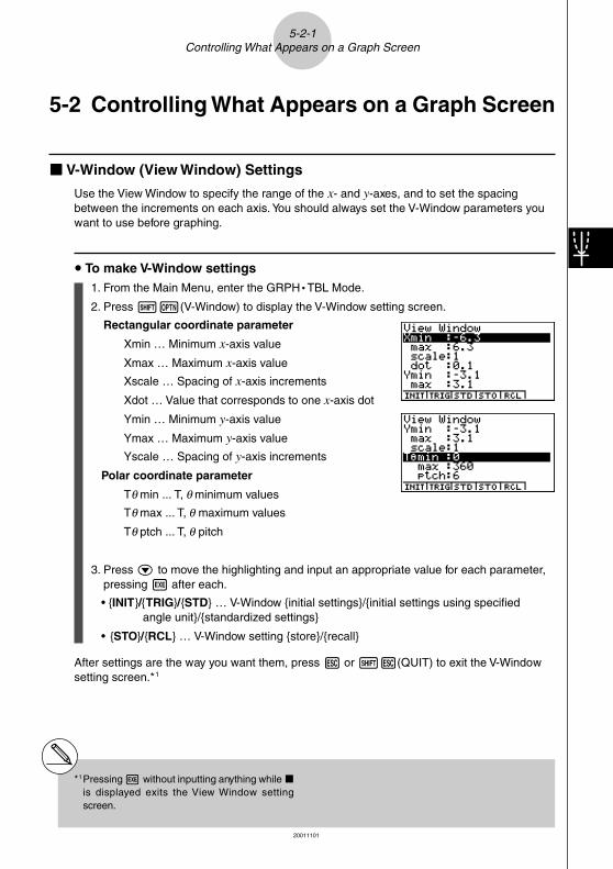
Use the View Window to specify the range of the x- and y-axes, and to set the spacingbetween the increments on each axis. You should always set the V-Window parameters youwant to use before graphing.
u To make V-Window settings1. From the Main Menu, enter the GRPH • TBL Mode.
2. Press !K(V-Window) to display the V-Window setting screen.
Rectangular coordinate parameter
Xmin … Minimum x-axis value
Xmax … Maximum x-axis value
Xscale … Spacing of x-axis increments
Xdot … Value that corresponds to one x-axis dot
Ymin … Minimum y-axis value
Ymax … Maximum y-axis value
Yscale … Spacing of y-axis increments
Polar coordinate parameter
Tθ min ... T, θ minimum values
Tθ max ... T, θ maximum values
Tθ ptch ... T, θ pitch
3. Press c to move the highlighting and input an appropriate value for each parameter,pressing w after each.
• {INIT}/{TRIG}/{STD} … V-Window {initial settings}/{initial settings using specifiedangle unit}/{standardized settings}
• {STO}/{RCL} … V-Window setting {store}/{recall}
After settings are the way you want them, press i or !i(QUIT) to exit the V-Windowsetting screen.*1
5-2-1Controlling What Appears on a Graph Screen
*1Pressing w without inputting anything while kis displayed exits the View Window settingscreen.
20011101
19990401
5-2-2Controlling What Appears on a Graph Screen
u V-Window Setting Precautions• Inputting zero for Tθ ptch causes an error.
• Any illegal input (out of range value, negative sign without a value, etc.) causes an error.
• An error occurs when Xmax is less than Xmin, or Ymax is less than Ymin. When Tθ maxis less than Tθ min, Tθ ptch becomes negative.
• You can input expressions (such as 2π) as V-Window parameters.
• When the V-Window setting produces an axis that does not fit on the display, the scaleof the axis is indicated on the edge of the display closest to the origin.
• Changing the V-Window settings clears the graph currently on the display andreplaces it with the new axes only.
• Changing the Xmin or Xmax value causes the Xdot value to be adjusted automatically.Changing the Xdot value causes the Xmax value to be adjusted automatically.
• A polar coordinate (r =) or parametric graph will appear coarse if the settings youmake in the V-Window cause the T, θ pitch value to be too large, relative to thedifferential between the T, θ min and T, θ max settings. If the settings you make causethe T, θ pitch value to be too small relative to the differential between the T, θ min andT, θ max settings, on the other hand, the graph will take a very long time to draw.
• The following is the input range for V-Window parameters.
–9.999999999E 97 to 9.999999999E 97

19990401
kkkkk Initializing and Standardizing the V-Window
u To initialize the V-Window1. From the Main Menu, enter the GRPH • TBL Mode.
2. Press !K(V-Window).
This displays the V-Window setting screen.
3. Press 1(INIT) to initialize the V-Window.
Xmin = –6.3, Xmax = 6.3, Xscale = 1 Xdot = 0.1
Ymin = –3.1, Ymax = 3.1, Yscale = 1
Tθ min = 0, Tθ max = 2π (rad), Tθ ptch = 2π /60 (rad)
u To initialize the V-Window in accordance with an angle unitIn step 3 of the procedure under “To initialize the V-Window” above, press 2(TRIG) toinitialize the V-Window in accordance with an angle unit.
Xmin = –3π (rad), Xmax = 3π (rad), Xscale = π /2 (rad), Xdot = π /21 (rad),
Ymin = –1.6, Ymax = 1.6, Yscale = 0.5
u To standardize the V-WindowThe following are the standard V-Window settings of this calculator.
Xmin = –10, Xmax = 10, Xscale = 1, Xdot = 0.15873015,
Ymin = –10, Ymax = 10, Yscale = 1,
Tθ min = 0, Tθ max = 2π (rad), Tθ ptch = 2π /60 (rad)
In step 3 of the procedure under “To initialize the V-Window” above, press 3(STD) tostandardize V-Window settings in accordance with the above.
5-2-3Controlling What Appears on a Graph Screen
# Initialization and standardization cause Tθmin, Tθ max, Tθ ptch values to changeautomatically in accordance with the currentangle unit setting as shown below.
Deg Mode:Tθ min = 0, Tθ max = 360, Tθ ptch = 6
Gra Mode:Tθ min = 0, Tθ max = 400, Tθ ptch = 400/60
20011101

19990401
kkkkk V-Window Memory
You can store up to six sets of V-Window settings in V-Window memory for recall when youneed them.
u To store V-Window settings1. From the Main Menu, enter the GRPH • TBL Mode.
2. Press !K(V-Window) to display the V-Window setting screen, and input the valuesyou want.
3. Press 4(STO) to display the pop-up window.
4. Press a number key to specify the V-Window memory where you want to save thesettings, and then press w. Pressing bw stores the settings in V-Window Memory1 (V-Win1).
u To recall V-Window memory settings1. From the Main Menu, enter the GRPH • TBL Mode.
2. Press !K(V-Window) to display the V-Window setting screen.
3. Press 5(RCL) to display the pop-up window.
4. Press a number key to specify the V-Window memory number for the settings you wantto recall, and then press w. Pressing bw recalls the settings in V-Window Memory1 (V-Win1).
5-2-4Controlling What Appears on a Graph Screen
# Storing V-Window settings to a memory thatalready contains setting data replaces theprevious data with the new settings.
# Recalling settings causes the current V-Windowsettings to be replaced with those recalled frommemory.
19990401
kkkkk Specifying the Graph Range
DescriptionYou can define a range (start point, end point) for a function before graphing it.
Set Up1. From the Main Menu, enter the GRPH • TBL Mode.
2. Make V-Window settings.
Execution3. Specify the function type and input the function. The following is the syntax for function
input.
Function ,!+( [ )Start Point , End Point !-( ] )
4. Draw the graph.
5-2-5Controlling What Appears on a Graph Screen

19990401
5-2-6Controlling What Appears on a Graph Screen
○ ○ ○ ○ ○
Example Graph y = x2 + 3x – 2 within the range – 2 < x < 4
Use the following V-Window settings.
Xmin = –3, Xmax = 5, Xscale = 1
Ymin = –10, Ymax = 30, Yscale = 5
Procedure1m GRPH • TBL
2!K(V-Window)-dwfwbwc
-bawdawfwi
33(TYPE)b(Y=)vx+dv-c,
!+( [ )-c,e!-( ] )w
45(DRAW)
Result Screen
# You can specify a range when graphingrectangular expressions, polar expressions,parametric functions, and inequalities.
19990401
5-2-7Controlling What Appears on a Graph Screen
kkkkk Zoom
DescriptionThis function lets you enlarge and reduce the graph on the screen.
Set Up1. Draw the graph.
Execution2. Specify the zoom type.
2(ZOOM)b(Box) ... Box zoomDraw a box around a display area, and that area is enlarged tofill the entire screen.
c(Factor)
d(In)/e(Out) ... Factor zoomThe graph is enlarged or reduced in accordance with the factoryou specify, centered on the current pointer location.
f(Auto) ...Auto zoomV-Window y-axis settings are automatically adjusted so thegraph fills the screen along the y-axis.
g(Orig) ...Original sizeReturns the graph to its original size following a zoom opera-tion.
h(Square) ... Graph correctionV-Window x-axis values are corrected so they are identical tothe y-axis values.
i(Rnd) ... Coordinate roundingRounds the coordinate values at the current pointer location.
j(Intg) ... IntegerEach dot is given a width of 1, which makes coordinate valuesintegers.
v(Pre) ...PreviousV-Window parameters are returned to what they were prior tothe last zoom operation.
l(QUICK) ... Quick zoomRedraws the graph in accordance with the settings stored in aselected V-Window memory.
Box zoom range specification
3. Use the cursor keys to move the pointer ( ) in the center of the screen to the locationwhere you want one corner of the box to be, and then press w.
4. Use the cursor keys to move the pointer. This causes a box to appear on the screen.Move the cursor until the area you want to enlarge is enclosed in the box, and thenpress w to enlarge it.
19990401
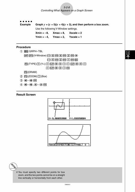
5-2-8Controlling What Appears on a Graph Screen
# You must specify two different points for boxzoom, and the two points cannot be on a straightline vertically or horizontally from each other.
○ ○ ○ ○ ○
Example Graph y = (x + 5)(x + 4)(x + 3), and then perform a box zoom.
Use the following V-Window settings.
Xmin = –8, Xmax = 8, Xscale = 2
Ymin = –4, Ymax = 2, Yscale = 1
Procedure1m GRPH • TBL
!K(V-Window)-iwiwcwc
-ewcwbwi
3(TYPE)b(Y=)(v+f)(v+e)
(v+d)w
5(DRAW)
22(ZOOM)b(Box)
3d~dw
4d~d,f~fw
Result Screen

19990401
5-2-9Controlling What Appears on a Graph Screen
kkkkk Factor Zoom
DescriptionWith factor zoom, you can zoom in or out, centered on the current cursor position.
Set Up1. Draw the graph.
Execution2. Press 2(ZOOM)c(Factor) to open a pop-up window for specifying the x-axis and
y-axis zoom factor. Input the values you want and then press i.
3. Press 2(ZOOM)d(In) to enlarge the graph, or 2(ZOOM)e(Out) to reduce it. Thegraph is enlarged or reduced centered on the current pointer location.
4. Use the cursor keys to move the cursor to the point upon which you want the zoomoperation to be centered, and then press w to zoom.
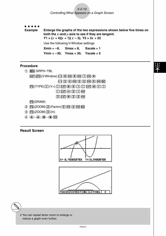
19990401
5-2-10Controlling What Appears on a Graph Screen
○ ○ ○ ○ ○
Example Enlarge the graphs of the two expressions shown below five times onboth the x-and y-axis to see if they are tangent.Y1 = (x + 4)(x + 1)( x – 3), Y2 = 3x + 22
Use the following V-Window settings.
Xmin = –8, Xmax = 8, Xscale = 1
Ymin = –30, Ymax = 30, Yscale = 5
Procedure1m GRPH • TBL
!K(V-Window)-iwiwbwc
-dawdawfwi
3(TYPE)b(Y=)(v+e)(v+b)
(v-d)w
dv+ccw
5(DRAW)
22(ZOOM)c(Factor)fwfwi
32(ZOOM)d(In)
4f~f,d~dw
Result Screen
# You can repeat factor zoom to enlarge orreduce a graph even further.

19990401
kkkkk Turning Function Menu Display On and Off
Press ua to toggle display of the menu at the bottom of the screen on and off.
Turning off the function menu display makes it possible to view part of a graph hidden behindit. When you are using the trace function or other functions during which the function menu isnormally not displayed, you can turn on the menu display to execute a menu command.
5-2-11Controlling What Appears on a Graph Screen
# If a pull-up menu is open when you press ua to turn off menu display, the pull-up menuremains on the screen.
20011101

19990401
kkkkk About the Calc Window
Pressing u4(CAT/CAL) while a graph or number table is on the display opens the CalcWindow. You can use the Calc Window to perform calculations with values obtained fromgraph analysis, or to change the value assigned to variable A in Y = AX and otherexpressions and then redraw the graph.
Press i to close the Calc Window.
5-2-12Controlling What Appears on a Graph Screen
# After using the Calc Window to change thevalue of a variable connected with a graph ortable, be sure to always execute Re-G (re-graph) or Re-T (re-calculate table). Doing soensures that the displayed graph or table iscurrent.
# Calc Window cannot be used in the RUN •MAT Mode while a program is running, or incombination with Dynamic Graph.
# Calc Window cannot be used in combinationwith V-Window or the table range setting screen.
# Complex number calculations cannot beperformed on the Calc Window.
20011101

19990401
5-3-1Drawing a Graph
5-3 Drawing a GraphYou can store up to 20 functions in memory. Functions in memory can be edited, recalled,and graphed.
kkkkk Specifying the Graph Type
Before you can store a graph function in memory, you must first specify its graph type.
1. While the Graph function list is on the display, press 6(g)3(TYPE) to display thegraph type menu, which contains the following items.
• {Y=}/{r=}/{Param}/{X=c} ... {rectangular coordinate}/{polar coordinate}/{parametric}/{X=constant}*1 graph
• {INEQUA}
• {Y>}/{Y<}/{Yttttt}/{Ysssss} ... {Y>f(x)}/{Y<f(x)}/{Y>f(x)}/{Y<f(x)} inequality graph
• {CONV}
• {'Y=}/{'Y>}/{'Y<}/{'Yttttt}/{'Ysssss} ... changes the function type
2. Press the number key that corresponds to the graph type you want to specify.
kkkkk Storing Graph Functions
u To store a rectangular coordinate function (Y =) *2
○ ○ ○ ○ ○
Example To store the following expression in memory area Y1 : y = 2x2 – 5
3(TYPE)b(Y =) (Specifies rectangular coordinate expression.)
cvx-f(Inputs expression.)
w (Stores expression.)
u To store a polar coordinate function (r =) *2
○ ○ ○ ○ ○
Example To store the following expression in memory area r2 : r = 5 sin3θ
3(TYPE)c(r =) (Specifies polar coordinate expression.)
fsdv(Inputs expression.)
w(Stores expression.)
*1 Attempting to draw a graph for an expressionin which X is input for an X = constantexpression results in an error.
*2 A function cannot be stored into a memory area thatalready contains a function of a different type fromthe one you are trying to store. Select a memoryarea that contains a function that is the same typeas the one you are storing, or delete the function inthe memory area to which you are trying to store.
20011101

19990401
5-3-2Drawing a Graph
u To store a parametric function *1
○ ○ ○ ○ ○
Example To store the following functions in memory areas Xt3 and Yt3 :x = 3 sin Ty = 3 cos T
3(TYPE)d(Param) (Specifies parametric expression.)
dsvw(Inputs and stores x expression.)
dcvw(Inputs and stores y expression.)
u To store an X = constant expression *2
○ ○ ○ ○ ○
Example To store the following expression in memory area X4 :X = 3
3(TYPE)e(X = c) (Specifies X = constant expression.)
d(Inputs expression.)
w(Stores expression.)
• Inputting X, Y, T, r, or θ for the constant in the above procedures causes an error.
u To store an inequality *2
○ ○ ○ ○ ○
Example To store the following inequality in memory area Y5 : y > x2 – 2x – 6
3(TYPE)f(INEQUA)b(Y>) (Specifies an inequality.)
vx-cv-g(Inputs expression.)
w(Stores expression.)
*1You will not be able to store the expression inan area that already contains a rectangularcoordinate expression, polar coordinateexpression, X = constant expression orinequality. Select another area to store yourexpression or delete the existing expressionfirst.
*2A function cannot be stored into a memory areathat already contains a function of a different typefrom the one you are trying to store. Select amemory area that contains a function that is thesame type as the one you are storing, or deletethe function in the memory area to which you aretrying to store.

19990401
5-3-3Drawing a Graph
u To create a composite function○ ○ ○ ○ ○
Example To register the following functions as a composite function:
Y1= (X + 1), Y2 = X2 + 3
Assign Y1°Y2 to Y3, and Y2°Y1 to Y4.
(Y1°Y2 = ((x2 + 3) +1) = (x2 + 4) Y2°Y1 = ( (X + 1)) 2 + 3 = X + 4 (X � –1))
3(TYPE)b(Y=)
J4(GRPH)b(Yn)b
(1(Yn)c)w
4(GRPH)b(Yn)c
(1(Yn)b)w
• A composite function can consist of up to five functions.
u To assign values to the coefficients and variables of a graph functionAfter you combine functions or equations into a composite function, you can assign values tothe coefficients and variables of the expression and draw a graph.
○ ○ ○ ○ ○
Example Assign the values –1, 0, and 1 to the expression Y = AX2 –1, which is inmemory area A
3(TYPE)b(Y=)
av(A)vx-bw
J4(GRPH)b(Yn)b
(av(A)!.(=)-b)w
4(GRPH)b(Yn)b
(av(A)!.(=)a)w
4(GRPH)b(Yn)b
(av(A)!.(=)b)w
20011101

19990401
ffffi1(SEL)5(DRAW)
The above three screens are produced using the Trace function.See “5-11 Function Analysis” for more information.
• If you do not specify a variable name (variable A in the above key operation), the calculatorautomatically uses one of the default variables listed below. Note that the default variableused depends on the memory area type where you are storing the graph function.
Memory Area Type Default Variable
Yn X
rn θXtn T
Ytn T
fn X
○ ○ ○ ○ ○
Example Y1 (3) and Y1 (X = 3) are identical values.
• You can also use Dynamic Graph for a look at how changes in coefficients alter theappearance of a graph. See “5-8 Dynamic Graphing” for more information.
5-3-4Drawing a Graph
20010102

1999040120011101
kkkkk Editing and Deleting Functions
u To edit a function in memory○ ○ ○ ○ ○
Example To change the expression in memory area Y1 from y = 2x2 – 5 toy = 2x2 – 3
e (Displays cursor.)
eeeeDd(Changes contents.)
w(Stores new graph function.)
u To change the type of a function*1
1. While the Graph function list is on the display, press f or c to move the highlightingto the area that contains the function whose type you want to change.
2. Press 3(TYPE)g(CONV).
3. Select the function type you want to change to.
○ ○ ○ ○ ○
Example To change the function in memory area Y1 from y = 2x2 – 3 toy < 2x2 – 3
3(TYPE)g(CONV)d('''''Y<) (Changes the function type to “Y<”.)
u To delete a function1. While the Graph function list is on the display, press f or c to move the highlighting
to the area that contains the function you want to delete.
2. Press 2(DEL) or D.
3. Press w(Yes) to delete the function or i(No) to abort the procedure without deletinganything.
*1The function type can be changed forrectangular coordinate functions andinequalities only.
# Parametric functions come in pairs (Xt and Yt).When editing a parametric function, clear the graphfunctions and re-input from the beginning.
5-3-5Drawing a Graph

1999040120011101
kkkkk Selecting Functions for Graphing
u To specify the draw/non-draw status of a graph○ ○ ○ ○ ○
Example To select the following functions for drawing :Y1 = 2x2 – 5, r2 = 5 sin3θUse the following V-Window settings.
Xmin = –5, Xmax = 5, Xscale = 1
Ymin = –5, Ymax = 5, Yscale = 1
Tθ min = 0, Tθ max = π, Tθ ptch = 2π / 60
cc (Select a memory area that contains a functionfor which you want to specify non-draw.)
1(SEL) (Specifies non-draw.)5(DRAW) or w (Draws the graphs.)
• Each press of 1(SEL) toggles a graph between draw and non-draw.
• Pressing u5(G↔T) or i returns to the Graph function list.
• You can use the SET UP screen settings to alter the appearance of the graph screen asshown below.
• Grid: On (Axes: On Label: Off)
This setting causes dots to appear at the gridintersects on the display.
• Axes: Off (Label: Off Grid: Off)
This setting clears the axis lines from the display.
• Label: On (Axes: On Grid: Off)
This setting displays labels for the x- and y-axes.
5-3-6Drawing a Graph

1999040120010102
kkkkkGraph Memory
Graph memory lets you store up to 20 sets of graph function data and recall it later when youneed it.
A single save operation saves the following data in graph memory.
• All graph functions in the currently displayed Graph function list (up to 20)
• Graph types
• Draw/non-draw status
• View Window settings (1 set)
u To store graph functions in graph memory1. Press 4(GMEM)b(Store) to display the pop-up window.
2. Press a number key to specify the Graph memory where you want to save the graphfunction, and then press w. Pressing bw stores the graph function to GraphMemory 1 (G-Mem1).
• There are 20 graph memories numbered G-Mem1 to G-Mem20.
u To recall a graph function1. Press 4(GMEM)c(Recall) to display the pop-up window.
2. Press a number key to specify the Graph memory for the function you want to recall,and then press w. Pressing bw recalls the graph function in Graph Memory 1(G-Mem1).
5-3-7Drawing a Graph
# Storing a function in a memory area thatalready contains a function replaces theexisting function with the new one.
# If the data exceeds the calculator’s remainingmemory capacity, an error occurs.
# Recalling data from graph memory causes anydata currently on the Graph function list to bedeleted.

19990401
5-4 Storing a Graph in Picture MemoryYou can save up to 20 graphic images in picture memory for later recall. You can overdrawthe graph on the screen with another graph stored in picture memory.
u To store a graph in picture memory1. After graphing in GRPH • TBL Mode, press 6(g)1(PICT)b(Store) to display the
pop-up window.
2. Press a number key to specify the Picture memory where you want to save the picture,and then press w. Pressing bw stores the picture function to Picture Memory 1(Pict 1).
• There are 20 picture memories numbered Pict 1 to Pict 20.
u To recall a stored graph1. After graphing in GRPH • TBL Mode, press 6(g)1(PICT)c(Recall) to display the
pop-up window.
2. Press a number key to specify the Picture memory for the picture you want to recall,and then press w. Pressing bw recalls the picture function in Picture Memory 1(Pict 1).
5-4-1Storing a Graph in Picture Memory
# Storing a graphic image in a memory area thatalready contains a graphic image replaces theexisting graphic image with the new one.
# A dual Graph screen or any other type of graphthat uses a split screen cannot be saved inpicture memory.

19990401
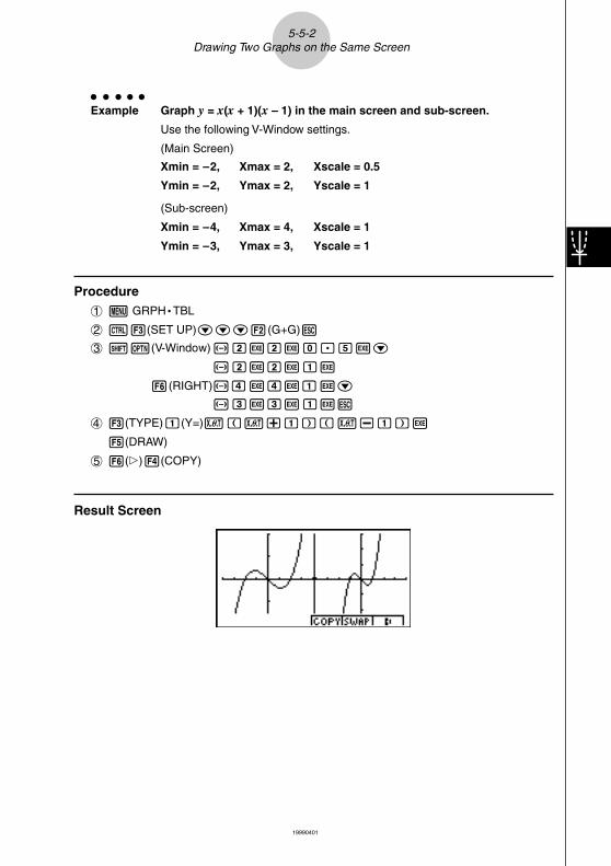
5-5 Drawing Two Graphs on the Same Screen
kkkkk Copying the Graph to the Sub-screen
DescriptionDual Graph lets you split the screen into two parts. Then you can graph two differentfunctions in each for comparison, or draw a normal size graph on one side and its enlargedversion on the other side. This makes Dual Graph a powerful graph analysis tool.
With Dual Graph, the left side of the screen is called the “main screen,” while the right side iscalled the “sub-screen.”
uuuuu Main ScreenThe graph in the main screen is actually drawn from a function.
uuuuu Sub-screenThe graph on the sub-screen is produced by copying or zooming the main screen graph.You can even make different V-Window settings for the sub-screen and main screen.
Set Up1. From the Main Menu, enter the GRPH • TBL Mode.
2. On the SET UP screen, select G+G for Dual Screen.
3. Make V-Window settings for the main screen.
Press 6(RIGHT) to display the sub-graph settings screen. Pressing 6(LEFT)returns to the main screen setting screen.
Execution4. Store the function, and draw the graph in the main screen.
5. Perform the Dual Graph operation you want.
4(COPY) ... Duplicates the main screen graph in the sub-screen
5(SWAP) ... Swaps the main screen contents and sub-screen contents
5-5-1Drawing Two Graphs on the Same Screen
19990401
○ ○ ○ ○ ○
Example Graph y = x(x + 1)(x – 1) in the main screen and sub-screen.
Use the following V-Window settings.
(Main Screen)
Xmin = –2, Xmax = 2, Xscale = 0.5
Ymin = –2, Ymax = 2, Yscale = 1
(Sub-screen)
Xmin = –4, Xmax = 4, Xscale = 1
Ymin = –3, Ymax = 3, Yscale = 1
Procedure1m GRPH • TBL
2u3(SET UP)ccc2(G+G)i
3!K(V-Window)-cwcwa.fwc
-cwcwbw
6(RIGHT)-ewewbwc
-dwdwbwi
43(TYPE)b(Y=)v(v+b)(v-b)w
5(DRAW)
56(g)4(COPY)
Result Screen
5-5-2Drawing Two Graphs on the Same Screen

19990401
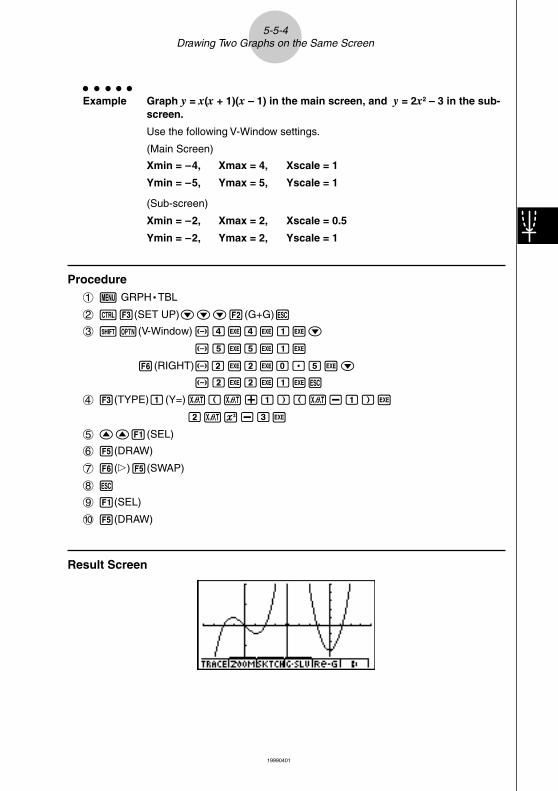
kkkkkGraphing Two Different Functions
DescriptionUse the following procedure to graph different functions in the main screen and sub-screen.
Set Up1. From the Main Menu, enter the GRPH • TBL Mode.
2. On the SET UP screen, select G+G for Dual Screen.
3. Make V-Window settings for the main screen.
Press 6(RIGHT) to display the sub-graph settings screen. Pressing 6(LEFT)returns to the main screen setting screen.
Execution4. Store the functions for the main screen and sub-screen.
5. Select the function of the graph that you want to eventually have in the sub-screen.
6. Draw the graph in the main screen.
7. Swap the main screen and sub-screen contents.
8. Return to the function screen.
9. Select the function of the next graph you want in the main screen.
10. Draw the graph in the main screen.
5-5-3Drawing Two Graphs on the Same Screen
19990401
○ ○ ○ ○ ○
Example Graph y = x(x + 1)(x – 1) in the main screen, and y = 2x2 – 3 in the sub-screen.
Use the following V-Window settings.
(Main Screen)
Xmin = –4, Xmax = 4, Xscale = 1
Ymin = –5, Ymax = 5, Yscale = 1
(Sub-screen)
Xmin = –2, Xmax = 2, Xscale = 0.5
Ymin = –2, Ymax = 2, Yscale = 1
Procedure1m GRPH • TBL
2u3(SET UP)ccc2(G+G)i
3!K(V-Window)-ewewbwc
-fwfwbw
6(RIGHT)-cwcwa.fwc
-cwcwbwi
43(TYPE)b(Y=)v(v+b)(v-b)w
cvx-dw
5ff1(SEL)
65(DRAW)
76(g)5(SWAP)
8i
91(SEL)
05(DRAW)
Result Screen
5-5-4Drawing Two Graphs on the Same Screen

19990401
kkkkk Using Zoom to Enlarge the Sub-screen
DescriptionUse the following procedure to enlarge the main screen graph and then move it to the sub-screen.
Set Up1. From the Main Menu, enter the GRPH • TBL Mode.
2. On the SET UP screen, select G+G for Dual Screen.
3. Make V-Window settings for the main screen.
Execution4. Input the function and draw the graph in the main screen.
5. Use Zoom to enlarge the graph, and then move it to the sub-screen.
5-5-5Drawing Two Graphs on the Same Screen

19990401
○ ○ ○ ○ ○
Example Draw the graph y = x(x + 1)(x – 1) in the main screen, and then useBox Zoom to enlarge it.
Use the following V-Window settings.
(Main Screen)
Xmin = –2, Xmax = 2, Xscale = 0.5
Ymin = –2, Ymax = 2, Yscale = 1
Procedure1m GRPH • TBL
2u3(SET UP)ccc2(G+G)i
3!K(V-Window)-cwcwa.fwc
-cwcwbwi
43(TYPE)b(Y=)v(v+b)(v-b)w
5(DRAW)
52(ZOOM)b(BOX)
c~ce~ew
f~fd~dw
Result Screen
5-5-6Drawing Two Graphs on the Same Screen

19990401
5-6-1Manual Graphing
5-6 Manual Graphing
kkkkk Rectangular Coordinate Graph
DescriptionInputting the Graph command in the RUN • MAT Mode enables drawing of rectangularcoordinate graphs.
Set Up1. From the Main Menu, enter the RUN • MAT Mode.
2. Make V-Window settings.
Execution3. Input the commands for drawing the rectangular coordinate graph.
4. Input the function.

19990401
5-6-2Manual Graphing
○ ○ ○ ○ ○
Example Graph y = 2x2 + 3x – 4
Use the following V-Window settings.
Xmin = –5, Xmax = 5, Xscale = 2
Ymin = –10, Ymax = 10, Yscale = 5
Procedure1m RUN • MAT
2!K(V-Window)-fwfwcwc
-bawbawfwi
3K6(g)6(g)2(SKTCH)b(Cls)w
2(SKTCH)e(GRAPH)b(Y=)
4 cvx+dv-ew
Result Screen
19991201

19990401
5-6-3Manual Graphing
kkkkk Integration Graph
DescriptionInputting the Graph command in the RUN • MAT Mode enables graphing of functionsproduced by an integration calculation.The calculation result is shown in the lower left of the display, and the calculation range isblackened in the graph.
Set Up1. From the Main Menu, enter the RUN • MAT Mode.
2. Make V-Window settings.
Execution3. Input graph commands for the integration graph.
4. Input the function.
19990401
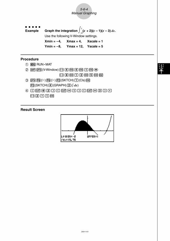
5-6-4Manual Graphing
○ ○ ○ ○ ○
Example Graph the integration ∫ (x + 2)(x – 1)(x – 3) dx.
Use the following V-Window settings.
Xmin = –4, Xmax = 4, Xscale = 1
Ymin = –8, Ymax = 12, Yscale = 5
Procedure1m RUN • MAT
2!K(V-Window)-ewewbwc
-iwbcwfwi
3K6(g)6(g)2(SKTCH)b(Cls)w
2(SKTCH)e(GRAPH)c(∫ dx)
4 (v+c)(v-b)(v-d),
-c,bw
Result Screen
1
–2
20011101

19990401
5-6-5Manual Graphing
kkkkk Drawing Multiple Graphs on the Same Screen
DescriptionUse the following procedure to assign various values to a variable contained in an expres-sion and overwrite the resulting graphs on the screen.
Set Up1. From the Main Menu, Enter GRPH • TBL Mode.
2. Make V-Window settings.
Execution3. Specify the function type and input the function. The following is the syntax for function
input.
Expression containing one variable ,!+( [ ) variable !.(=)
value , value , ... , value !-( ] )
4. Draw the graph.
19990401
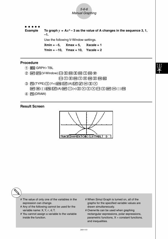
5-6-6Manual Graphing
○ ○ ○ ○ ○
Example To graph y = Ax2 – 3 as the value of A changes in the sequence 3, 1,–1.
Use the following V-Window settings.
Xmin = –5, Xmax = 5, Xscale = 1
Ymin = –10, Ymax = 10, Yscale = 2
Procedure1m GRPH • TBL
2!K(V-Window)-fwfwbwc
-bawbawcwi
33(TYPE)b(Y=)av(A)vx-d,
!+( [ )av(A)!.(=)d,b,-b!-( ] )w
45(DRAW)
Result Screen
# The value of only one of the variables in theexpression can change.
# Any of the following cannot be used for thevariable name: X, Y, r, θ, T.
# You cannot assign a variable to the variableinside the function.
# When Simul Graph is turned on, all of thegraphs for the specified variable values aredrawn simultaneously.
# Overwrite can be used when graphingrectangular expressions, polar expressions,parametric functions, X = constant functions,and inequalities.
20011101

19990401
5-7 Using Tables
kkkkk Storing a Function and Generating a Number Table
u To store a function○ ○ ○ ○ ○
Example To store the function y = 3x2 – 2 in memory area Y1
Use f and c to move the highlighting in the Graph function list to the memory areawhere you want to store the function. Next, input the function and press w to store it.
uVariable SpecificationsThere are two methods you can use to specify value for the variable x when generating anumeric table.
• Table range method
With this method, you specify the conditions for the change in value of the variable.
• List
With this method, the data in the list you specify is substituted for the x-variable togenerate a number table.
u To generate a table using a table range○ ○ ○ ○ ○
Example To generate a table as the value of variable x changes from –3 to 3, inincrements of 1
6(g)2(RANG)
-dwdwbw
The numeric table range defines the conditions under which the value of variable x changesduring function calculation.
Start ........... Variable x start value
End ............. Variable x end value
pitch ............ Variable x value change (interval)
After specifying the table range, press i to return to the Graph function list.
5-7-1Using Tables

19990401
u To generate a table using a list1. While the Graph function list is on the screen, display the SET UP screen.
2. Highlight Variable and then press 2(LIST) to display the pop-up window.
3. Select the list whose values you want to assign for the x-variable. • To select List 6, for example, press gw. This causes the setting of the Variable item
of the SET UP screen to change to List 6.
4. After specifying the list you want to use, press i to return to the previous screen.
• Note that the {RANG} item does not appear when a list name is specified for the Variable item of the SET UP screen.
uGenerating a Table○ ○ ○ ○ ○
Example To generate a table of values for the functions stored in memory areasY1 and Y3 of the Graph function list
Use f and c to move the highlighting to the function you want to select for table genera-tion and press 1(SEL) to select it.
The “=” sign of selected functions is highlighted on the screen. To deselect a function, movethe cursor to it and press 1(SEL) again.
Press 5(TABL) to generate a number table using the functions you selected. The value ofvariable x changes according to the range or the contents of the list you specified.
The example screen shown here shows the resultsbased on the contents of List 6 (– 3, –2, –1, 0, 1, 2, 3).
Each cell can contain up to six digits, including negative sign.
5-7-2Using Tables
19990401
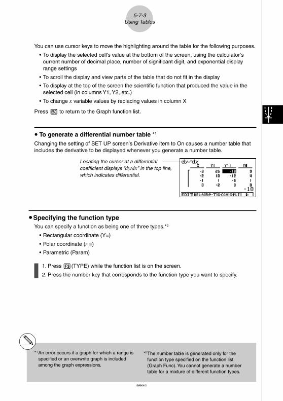
You can use cursor keys to move the highlighting around the table for the following purposes.
• To display the selected cell’s value at the bottom of the screen, using the calculator’scurrent number of decimal place, number of significant digit, and exponential displayrange settings
• To scroll the display and view parts of the table that do not fit in the display
• To display at the top of the screen the scientific function that produced the value in theselected cell (in columns Y1, Y2, etc.)
• To change x variable values by replacing values in column X
Press i to return to the Graph function list.
u To generate a differential number table *1
Changing the setting of SET UP screen’s Derivative item to On causes a number table thatincludes the derivative to be displayed whenever you generate a number table.
uSpecifying the function typeYou can specify a function as being one of three types.*2
• Rectangular coordinate (Y=)
• Polar coordinate (r =)
• Parametric (Param)
1. Press 3(TYPE) while the function list is on the screen.
2. Press the number key that corresponds to the function type you want to specify.
5-7-3Using Tables
Locating the cursor at a differentialcoefficient displays “dy/dx” in the top line,which indicates differential.
*1An error occurs if a graph for which a range isspecified or an overwrite graph is includedamong the graph expressions.
*2The number table is generated only for thefunction type specified on the function list(Graph Func). You cannot generate a numbertable for a mixture of different function types.
19990401
kkkkk Editing and Deleting Functions
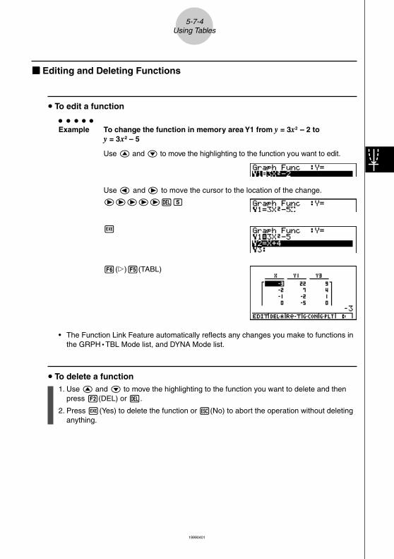
u To edit a function○ ○ ○ ○ ○
Example To change the function in memory area Y1 from y = 3x2 – 2 toy = 3x2 – 5
Use f and c to move the highlighting to the function you want to edit.
Use d and e to move the cursor to the location of the change.
eeeeeDf
w
6(g)5(TABL)
• The Function Link Feature automatically reflects any changes you make to functions inthe GRPH • TBL Mode list, and DYNA Mode list.
u To delete a function1. Use f and c to move the highlighting to the function you want to delete and then
press 2(DEL) or D.
2. Press w(Yes) to delete the function or i(No) to abort the operation without deletinganything.
5-7-4Using Tables
19990401
5-7-5Using Tables
kkkkk Editing Tables
You can use the table menu to perform any of the following operations once you generate atable.
• Change the values of variable x
• Edit (delete, insert, and append) rows
• Delete a table and regenerate table
• Draw a connect type graph
• Draw a plot type graph
While the Table & Graph menu is on the display, press 3(TABL) to display the table menu.
• {EDIT} ... {edit value of x-variable}
• {DEL·A} ... {delete table}
• {Re-T} ... {regenerate table from function}
• {G·CON}/{G·PLT} ... {connected type}/{draw plot type} graph draw
• {R·DEL}/{R·INS} /{R·ADD} ... {delete}/{insert}/{add} row
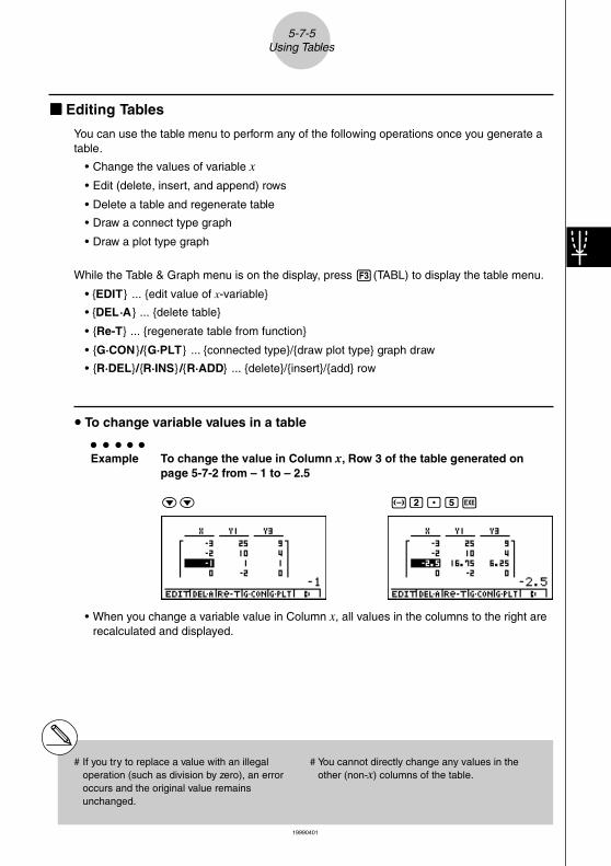
u To change variable values in a table○ ○ ○ ○ ○
Example To change the value in Column x, Row 3 of the table generated onpage 5-7-2 from – 1 to – 2.5
cc -c.fw
• When you change a variable value in Column x, all values in the columns to the right arerecalculated and displayed.
# If you try to replace a value with an illegaloperation (such as division by zero), an erroroccurs and the original value remainsunchanged.
# You cannot directly change any values in theother (non-x) columns of the table.

19990401
5-7-6Using Tables
uRow Operations
u To delete a row○ ○ ○ ○ ○
Example To delete Row 2 of the table generated on page 5-7-2
c 6(g)1(R·DEL)
u To insert a row○ ○ ○ ○ ○
Example To insert a new row between Rows 1 and 2 in the table generated onpage 5-7-2
c 6(g)2(R·INS)

19990401
5-7-7Using Tables
u To add a row○ ○ ○ ○ ○
Example To add a new row below Row 7 in the table generated on page 5-7-2
cccccc 6(g)3(R·ADD)
uDeleting a Table1. Display the table and then press 2(DEL·A).
2. Press w(Yes) to delete the table or i(No) to abort the operation without deletinganything.

19990401
kkkkk Copying a Table Column to a List
A simple operation lets you copy the contents of a numeric table column into a list.
u To copy a table to a list○ ○ ○ ○ ○
Example To copy the contents of Column x into List 1
K1(LMEM)
• You can select any row of the column you want to copy.
Input the number of the list you want to copy and then press w.
bw
5-7-8Using Tables

19990401
kkkkkDrawing a Graph from a Number Table
DescriptionUse the following procedure to generate a number table and then draw a graph based on thevalues in the table.
Set Up1. From the Main Menu, enter the GRPH • TBL Mode.
2. Make V-Window settings.
Execution3. Store the functions.
4. Specify the table range.
5. Generate the table.
6. Select the graph type and draw it.
4(G • CON) ... line graph*1
5(G • PLT) ... plot type graph*1*2
5-7-9Using Tables
*1After drawing the graph, pressing u5(G ↔ T) or i returns to the functionstorage screen. To return to the number tablescreen, press 5(TABL).
*2Pressing 6(g) 4(G • PLT) on the functionstorage screen generates the number tableand plots the graph simultaneously.
19990401
○ ○ ○ ○ ○
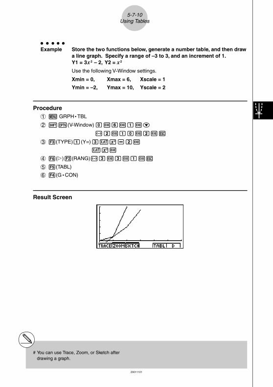
Example Store the two functions below, generate a number table, and then drawa line graph. Specify a range of –3 to 3, and an increment of 1.Y1 = 3x2 – 2, Y2 = x2
Use the following V-Window settings.
Xmin = 0, Xmax = 6, Xscale = 1
Ymin = –2, Ymax = 10, Yscale = 2
Procedure1m GRPH • TBL
2!K(V-Window)awgwbwc
-cwbawcwi
33(TYPE)b(Y=)dvx-cw
vxw
46(g)2(RANG)-dwdwbwi
55(TABL)
64(G • CON)
Result Screen
5-7-10Using Tables
# You can use Trace, Zoom, or Sketch afterdrawing a graph.
20011101

19990401
kkkkk Specifying a Range for Number Table Generation
DescriptionUse the following procedure to specify a number table range when calculating scatter datafrom a function.
Set Up1. From the Main Menu, enter the GRPH • TBL Mode.
Execution2. Store the functions.
3. Specify the table range.
4. Select the functions for which you want to generate a table.
The “=” sign of selected functions is highlighted on the screen.
5. Generate the table.
5-7-11Using Tables
19990401
○ ○ ○ ○ ○
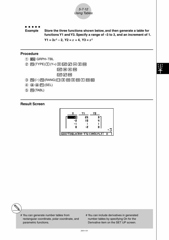
Example Store the three functions shown below, and then generate a table forfunctions Y1 and Y3. Specify a range of –3 to 3, and an increment of 1.
Y1 = 3x2 – 2, Y2 = x + 4, Y3 = x2
Procedure1m GRPH • TBL
23(TYPE)b(Y=)dvx-cw
v+ew
vxw
36(g)2(RANG)-dwdwbwi
4ff1(SEL)
55(TABL)
Result Screen
5-7-12Using Tables
# You can generate number tables fromrectangular coordinate, polar coordinate, andparametric functions.
# You can include derivatives in generatednumber tables by specifying On for theDerivative item on the SET UP screen.
20011101

19990401
kkkkk Simultaneously Displaying a Number Table and Graph
DescriptionSpecifying T+G for Dual Screen on the SET UP makes it possible to display a number tableand graph at the same time.
Set Up1. From the Main Menu, enter the GRPH • TBL Mode.
2. Make V-Window settings.
3. On the SET UP screen, select T+G for Dual Screen.
Execution4. Input the function.
5. Specify the table range.
6. The number table is displayed in the sub-screen on the right.
7. Specify the graph type and draw the graph.
4(G • CON) ... line graph
5(G • PLT) ... plot type graph*1
5-7-13Using Tables
*1Pressing 6(g) 4(G • PLT) on the functionstorage screen generates the number tableand plots the graph simultaneously.

19990401
○ ○ ○ ○ ○
Example Store the function Y1 = 3x2 – 2 and simultaneously display its numbertable and line graph. Use a table range of –3 to 3 with an increment of 1.
Use the following V-Window settings.
Xmin = 0, Xmax = 6, Xscale = 1
Ymin = –2, Ymax = 10, Yscale = 2
Procedure1m GRPH • TBL
2!K(V-Window)awgwbwc
-cwbawcwi
3u3(SET UP)ccc1(T+G)i
43(TYPE)b(Y=)dvx-cw
56(g)2(RANG)
-dwdwbwi
65(TABL)
74(G • CON)
Result Screen
5-7-14Using Tables
20011101

19990401
5-7-15Using Tables
kkkkk Using Graph-Table Linking
DescriptionWith Dual Graph, you can use the following procedure to link the graph and table screens sothe pointer on the graph screen jumps to the location of the currently selected table value.
Set Up1. From the Main Menu, enter the GRPH • TBL Mode.
2. Make the required V-Window settings.
Display the SET UP screen, select the Dual Screen item, and change its setting to“T+G”.
Execution3. Input the function of the graph and make the required table range settings.
4. With the number table on the right side of the display, draw the graph on the left side.
4(G • CON) ... connect type graph
5(G • PLT) ... plot type graph
5. Turn on G • Link.
6. Now when you use c and f to move the highlighting among the cells in the table,the pointer jumps to the corresponding point on the graph screen.If there are multiple graphs, pressing d and e causes the pointer to jump betweenthem.
To turn off G • Link, press i or !i(QUIT).

19990401
5-7-16Using Tables
○ ○ ○ ○ ○
Example Store the function Y1 = 3logx and simultaneously display its numbertable and plot-type graph. Use a table range of 2 through 9, with anincrement of 1.
Use the following V-Window settings.
Xmin = –1, Xmax = 10, Xscale = 1
Ymin = –1, Ymax = 4, Yscale = 1
Procedure1m GRPH • TBL
2!K(V-Window)-bwbawbwc
-bwewbwi
u3(SET UP)ccc1(T+G)i
33(TYPE)b(Y=)dlvw
6(g)2(RANG)
cwjwbwi
45(TABL)
5(G • PLT)
56(g)4(G • Link)
6c ~ c, f ~ f
Result Screen
…→←…

19990401
5-8 Dynamic Graphing
kkkkk Using Dynamic Graph
DescriptionDynamic Graph lets you define a range of values for the coefficients in a function, and thenobserve how a graph is affected by changes in the value of a coefficient. It helps to see howthe coefficients and terms that make up a function influence the shape and position of agraph.
Set Up1. From the Main Menu, enter the DYNA Mode.
2. Make V-Window settings.
Execution3. On the SET UP screen, specify the Dynamic Type.
1(Cont) ... Continuous
2(Stop) ... Automatic stop after 10 draws
4. Use the cursor keys to select the function type on the built-in function type list.*1
5. Input values for coefficients, and specify which coefficient will be the dynamic vari-able.*2
6. Specify the start value, end value, and increment.
7. Specify the drawing speed.
3(SPEED)1( ) .....Pause after each draw (Stop & Go)
2( ) .......Half normal speed (Slow)
3( ) .......Normal speed (Normal)
4( ) ...... Twice normal speed (Fast)
8. Draw the Dynamic Graph.
5-8-1Dynamic Graphing
*1The following are the seven built-in functiontypes.
•Y=AX+B•Y=A(X–B)2+C•Y=AX2+BX+C•Y=AX^3+BX2+CX+D•Y=Asin(BX+C)•Y=Acos(BX+C)•Y=Atan(BX+C)
After you press 3(TYPE) and select thefunction type you want, you can then input theactual function.
b ... rectangular coordinate expressionc ... polar coordinate expressiond ... parametric function
*2You could also press w here and display theparameter setting menu.
# The message “Too Many Functions” appearswhen more than one function is selected forDynamic Graphing.

19990401
○ ○ ○ ○ ○
Example Use Dynamic Graph to graph y = A (x – 1)2 – 1, in which the value ofcoefficient A changes from 2 through 5 in increments of 1. The Graphis drawn 10 times.
Use the following V-Window settings.
Xmin = –6.3, Xmax = 6.3, Xscale = 1
Ymin = –3.1, Ymax = 3.1, Yscale = 1 (initial defaults)
Procedure1m DYNA
2!K(V-Window)1(INIT)i
3u3(SET UP)2(Stop)i
46(g)3(B-IN)c1(SEL)
56(g)4(VAR)cwbw-bw
62(RANG)cwfwbwi
73(SPEED)3( ) i
86(DYNA)
Result Screen
↓
→←
↓↑
→←
5-8-2Dynamic Graphing
1
4
2
3
Repeats from 1 through 4.

19990401
kkkkk Dynamic Graph Application Examples
DescriptionYou can also use Dynamic Graph to simulate simple physical phenomena.
Set Up1. From the Main Menu, enter the DYNA Mode.
2. Make V-Window settings.
Execution3. On the SET UP screen, specify Stop for Dynamic Type and Deg for Angle.
4. Specify Param (parametric function) as the function type, and input a function thatcontains a dynamic variable.
5. Specify the dynamic coefficient.
6. Specify the start value, end value, and increment.
7. Specify Normal for the draw speed.
8. Start the Dynamic Graph operation.
5-8-3Dynamic Graphing
19990401
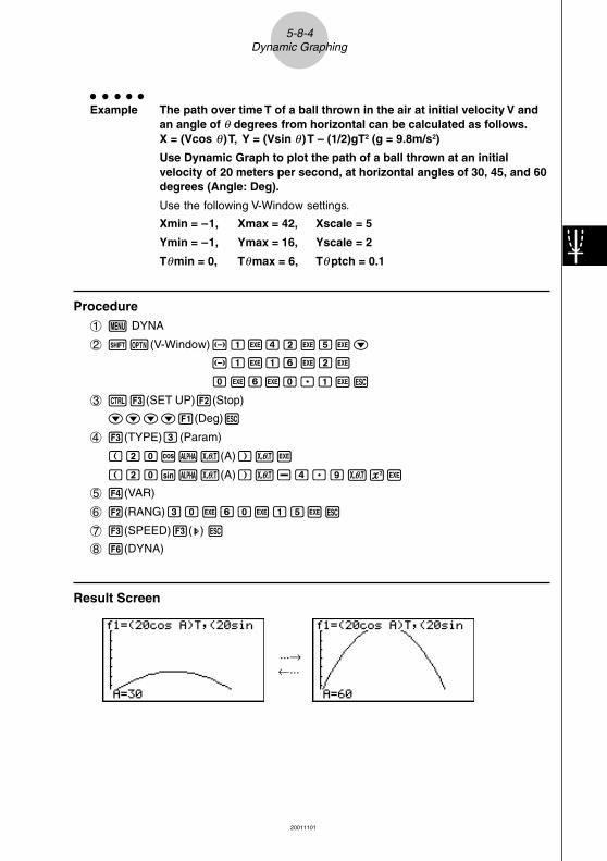
○ ○ ○ ○ ○
Example The path over time T of a ball thrown in the air at initial velocity V andan angle of θ degrees from horizontal can be calculated as follows.X = (Vcos θ )T, Y = (Vsin θ )T – (1/2)gT2 (g = 9.8m/s2)
Use Dynamic Graph to plot the path of a ball thrown at an initialvelocity of 20 meters per second, at horizontal angles of 30, 45, and 60degrees (Angle: Deg).
Use the following V-Window settings.
Xmin = –1, Xmax = 42, Xscale = 5
Ymin = –1, Ymax = 16, Yscale = 2
Tθmin = 0, Tθmax = 6, Tθ ptch = 0.1
Procedure1m DYNA
2!K(V-Window)-bwecwfwc
-bwbgwcw
awgwa.bwi
3u3(SET UP)2(Stop)
cccc1(Deg)i
43(TYPE)d(Param)
(cacav(A))vw
(casav(A))v-e.jvxw
54(VAR)
62(RANG)dawgawbfwi
73(SPEED)3( ) i
86(DYNA)
Result Screen
···→←···
5-8-4Dynamic Graphing
2001100120011101
19990401
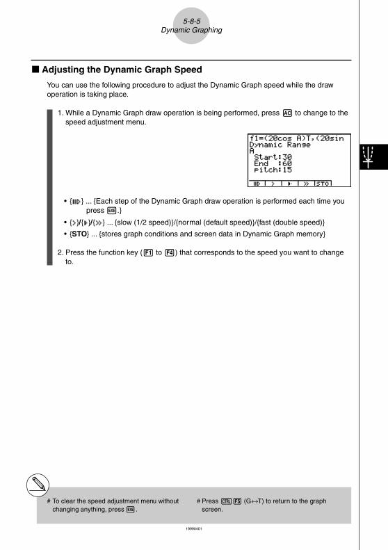
k Adjusting the Dynamic Graph Speed
You can use the following procedure to adjust the Dynamic Graph speed while the drawoperation is taking place.
1. While a Dynamic Graph draw operation is being performed, press A to change to thespeed adjustment menu.
• { } ... {Each step of the Dynamic Graph draw operation is performed each time youpress w.}
• { }/{ }/{ } ... {slow (1/2 speed)}/{normal (default speed)}/{fast (double speed)}
• {STO} ... {stores graph conditions and screen data in Dynamic Graph memory}
2. Press the function key (1 to 4) that corresponds to the speed you want to changeto.
5-8-5Dynamic Graphing
# To clear the speed adjustment menu withoutchanging anything, press w.
# Press u5 (G↔T) to return to the graphscreen.
19990401
kkkkk Using Dynamic Graph Memory
You can store Dynamic Graph conditions and screen data in Dynamic Graph memory forlater recall when you need it. This lets you save time, because you can recall the data andimmediately begin a Dynamic Graph draw operation. Note that you can store one set of datain memory at any one time.
The following is all of the data that makes up a set.
• Graph functions (up to 20)
• Dynamic Graph conditions
• SET UP screen settings
• V-Window contents
• Dynamic Graph screen
uuuuu To save data in Dynamic Graph memory1. While a Dynamic Graph draw operation is being performed, press A to change to the
speed adjustment menu.
2. Press 5(STO). In response to the confirmation dialog that appears, press w(Yes) tosave the data.
uuuuu To recall data from Dynamic Graph memory1. Display the Dynamic Graph function list.
2. Press 6(RCL) to recall all the data stored in Dynamic Graph memory.
5-8-6Dynamic Graphing
# If there is already data stored in DynamicGraph memory, the data save operationreplaces it with the new data.
# Data recalled from Dynamic Graph memoryreplaces the calculator’s current graph functions,draw conditions, and screen data. The previousdata is lost when it is replaced.

19990401
5-9 Graphing a Recursion Formula
kkkkkGenerating a Number Table from a Recursion Formula
DescriptionYou can input up to three of the following types of recursion formulas and generate a numbertable.
• General term of sequence {an}, composed of an, n
• Linear two-term recursion composed of an+1, an, n
• Linear three-term recursion composed of an+2, an+1, an, n
Set Up1. From the Main Menu, enter the RECUR Mode.
Execution2. Specify the recursion type.
3(TYPE)b(an=) ... {general term of sequence an}
c(an+1=) ... {linear two-term recursion}
d(an+2=) ... {linear three-term recursion}
3. Input the recursion formula.
4. Specify the table range. Specify a start point and end point for n. If necessary, specify avalue for the initial term, and a pointer start point value if you plan to graph the formula.
5. Display the recursion formula number table.
5-9-1Graphing a Recursion Formula
19990401
○ ○ ○ ○ ○
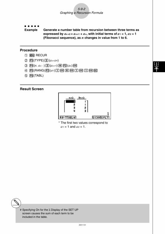
Example Generate a number table from recursion between three terms asexpressed by an+2 = an+1 + an, with initial terms of a1 = 1, a2 = 1(Fibonacci sequence), as n changes in value from 1 to 6.
Procedure1m RECUR
23(TYPE)d(an+2=)
34(n. an ··)d(an+1)+2(an)w
45(RANG)2(a1)bwgwbwbwi
56(TABL)
Result Screen
5-9-2Graphing a Recursion Formula
# Specifying On for the Σ Display of the SET UPscreen causes the sum of each term to beincluded in the table.
* The first two values correspond toa1 = 1 and a2 = 1.
20011101
19990401
kkkkkGraphing a Recursion Formula (1)
DescriptionAfter generating a number table from a recursion formula, you can graph the values on a linegraph or plot type graph.
Set Up1. From the Main Menu, enter the RECUR Mode.
2. Make V-Window settings.
Execution3. Specify the recursion formula type and input the formula.
4. Specify the table range, and start and ending values for n. If necessary, specify theinitial term value and pointer start point.
5. Display the recursion formula number table.
6. Specify the graph type and draw the graph.
5(G • CON) ... line graph
6(G • PLT) ... plot type graph
5-9-3Graphing a Recursion Formula

19990401
○ ○ ○ ○ ○
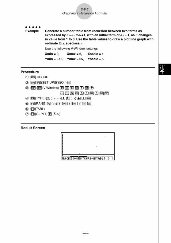
Example Generate a number table from recursion between two terms asexpressed by an+1 = 2an+1, with an initial term of a1 = 1, as n changesin value from 1 to 6. Use the table values to draw a line graph.
Use the following V-Window settings.
Xmin = 0, Xmax = 6, Xscale = 1
Ymin = –15, Ymax = 65, Yscale = 5
Procedure1m RECUR
2!K(V-Window)awgwbwc
-bfwgfwfwi
33(TYPE)c(an+1=)c2(an)+bw
45(RANG)2(a1)bwgwbwi
56(TABL)
65(G • CON)
Result Screen
5-9-4Graphing a Recursion Formula

19990401
kkkkkGraphing a Recursion Formula (2)
DescriptionThe following describes how to generate a number table from a recursion formula and graphthe values while Σ Display is On.
Set Up1. From the Main Menu, enter the RECUR Mode.
2. On the SET UP screen, specify On for Σ Display.
3. Make V-Window settings.
Execution4. Specify the recursion formula type and input the recursion formula.
5. Specify the table range, and start and ending values for n. If necessary, specify theinitial term value and pointer start point.
6. Display the recursion formula number table.
7. Specify the graph type and draw the graph.
5(G • CON)b(an) ... Line graph with ordinate an, abscissa n
c(Σan) ... Line graph with ordinate Σan, abscissa n
6(G • PLT) b(an) ... Plot type graph with ordinate an, abscissa n
c(Σan) ... Plot type graph with ordinate Σan, abscissa n
5-9-5Graphing a Recursion Formula
19990401
○ ○ ○ ○ ○
Example Generate a number table from recursion between two terms asexpressed by an+1 = 2an+1, with an initial term of a1 = 1, as n changesin value from 1 to 6. Use the table values to draw a plot line graph withordinate Σan, abscissa n.
Use the following V-Window settings.
Xmin = 0, Xmax = 6, Xscale = 1
Ymin = –15, Ymax = 65, Yscale = 5
Procedure1m RECUR
2u3(SET UP)1(On)i
3!K(V-Window)awgwbwc
-bfwgfwfwi
43(TYPE)c(an+1=)c2(an)+bw
55(RANG)2(a1)bwgwbwi
66(TABL)
76(G • PLT)c(Σan)
Result Screen
5-9-6Graphing a Recursion Formula

19990401
kkkkkWEB Graph (Convergence, Divergence)
Descriptiony = f(x) is graphed by presuming an+1 = y, an = x for linear two-term regression an+1 = f(an)composed of an+1, an. Next, it can be determined whether the function is convergent ordivergent.
Set Up1. From the Main Menu, enter the RECUR Mode.
2. Make V-Window settings.
Execution3. Select 2-term recursion as the recursion formula type, and input the formula.
4. Specify the table range, n start and end points, initial term value, and pointer startpoint.
5. Display the recursion formula number table.
6. Draw the graph.
7. Press w, and the pointer appears at the start point you specified.Press w several times.
If convergence exists, lines that resemble a spider web are drawn on the display.Failure of the web lines to appear indicates either divergence or that the graph isoutside the boundaries of the display screen. When this happens, change to largerView Window values and try again.
You can use fc to select the graph.
5-9-7Graphing a Recursion Formula
19990401
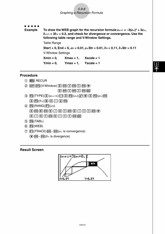
○ ○ ○ ○ ○
Example To draw the WEB graph for the recursion formula an+1 = –3(an)2 + 3an,bn+1 = 3bn + 0.2, and check for divergence or convergence. Use thefollowing table range and V-Window Settings.
Table Range
Start = 0, End = 6, a0 = 0.01, anStr = 0.01, b0 = 0.11, bnStr = 0.11
V-Window Settings
Xmin = 0, Xmax = 1, Xscale = 1
Ymin = 0, Ymax = 1, Yscale = 1
Procedure1m RECUR
2!K(V-Window)awbwbwc
awbwbwi
33(TYPE)c(an+1=)-d2(an)x+d2(an)w
d3(bn)+a.cw
45(RANG)1(a0)
awgwa.abwa.bbwc
a.abwa.bbwi
56(TABL)
64(WEB)
71(TRACE)w~w(an is convergence)
cw~w(bn is divergence)
Result Screen
5-9-8Graphing a Recursion Formula

19990401
5-10-1Changing the Appearance of a Graph
5-10 Changing the Appearance of a Graph
kkkkk Drawing a Line
DescriptionThe sketch function lets you draw points and lines inside of graphs.
Set Up1. Draw the graph.
Execution2. Select the sketch function you want to use.*1
3(SKTCH)b(Cls) ... Screen clear
c(PLOT){On}/{Off}/{Change}/{Plot} ... Point {On}/{Off}/{Change}/{Plot}
d(LINE){F-Line}/{Line} ... {Freehand line}/{Line}
e(Text) ... Text input
f(Pen) ... Freehand
g(Tangnt) ... Tangent line
h(Normal) ... Line normal to a curve
i(Invrse) ... Inverse function*2
j(Circle) ... Circle
v(Vert) ... Vertical line
l(Horz) ... Horizontal line
3. Use the cursor keys to move the pointer ( ) to the location where you want to draw,and press w.*3
*1The above shows the function menu thatappears in the GRPH • TBL Mode. Menu itemsmay differ somewhat in other modes.
*2 In the case of an inverse function graph,drawing starts immediately after you selectthis option.
*3Some sketch functions require specification oftwo points. After you press w to specify thefirst point, use the cursor keys to move thepointer to the location of the second point andpress w.
19990401
○ ○ ○ ○ ○
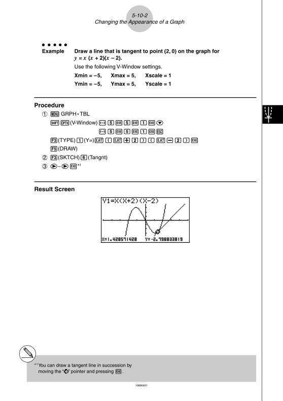
Example Draw a line that is tangent to point (2, 0) on the graph fory = x (x + 2)(x – 2).
Use the following V-Window settings.
Xmin = –5, Xmax = 5, Xscale = 1
Ymin = –5, Ymax = 5, Yscale = 1
Procedure1m GRPH • TBL
!K(V-Window)-fwfwbwc
-fwfwbwi
3(TYPE)b(Y=)v(v+c)(v-c)w
5(DRAW)
23(SKTCH)g(Tangnt)
3e~ew*1
Result Screen
5-10-2Changing the Appearance of a Graph
*1You can draw a tangent line in succession bymoving the “ ” pointer and pressing w.

19990401
kkkkk Inserting Comments
DescriptionYou can insert comments anywhere you want in a graph.
Set Up1. Draw the graph.
Execution2. Press 3(SKTCH)e(Text), and a pointer appears in the center of the display.
3. Use the cursor keys to move the pointer to the location where you want the text to be,and input the text.
5-10-3Changing the Appearance of a Graph
# You can input any of the following characters ascomment text: A~Z, r, θ, space, 0~9, ., +, –, ×,÷, (–), EXP, π, Ans, (, ), [, ], {, }, comma, →,
x2, ^, log, In, , x , 10x, ex, 3 , x–1, sin, cos,tan, sin–1, cos–1, tan–1, i, List, Mat
19990401
○ ○ ○ ○ ○
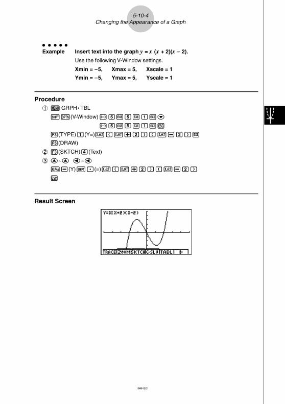
Example Insert text into the graph y = x (x + 2)(x – 2).
Use the following V-Window settings.
Xmin = –5, Xmax = 5, Xscale = 1
Ymin = –5, Ymax = 5, Yscale = 1
Procedure1m GRPH • TBL
!K(V-Window)-fwfwbwc
-fwfwbwi
3(TYPE)b(Y=)v(v+c)(v-c)w
5(DRAW)
23(SKTCH)e(Text)
3f~f d~d
a-(Y)!.(=)v(v+c)(v-c)
i
Result Screen
5-10-4Changing the Appearance of a Graph
19991201

19990401
kkkkk Freehand Drawing
DescriptionYou can use the pen option for freehand drawing in a graph.
Set Up1. Draw the graph.
Execution2. Press 3(SKTCH)f(Pen), and a pointer appears in the center of the screen.
3. Use the cursor keys to move the pointer to the point from which you want to startdrawing, and then press w.
4. Use the cursor keys to move the pointer. A line is drawn wherever you move the pointer.To stop the line, press w.
Repeat step 3 and 4 to draw other lines.
After you are finished drawing, press i.
5-10-5Changing the Appearance of a Graph
19990401
○ ○ ○ ○ ○
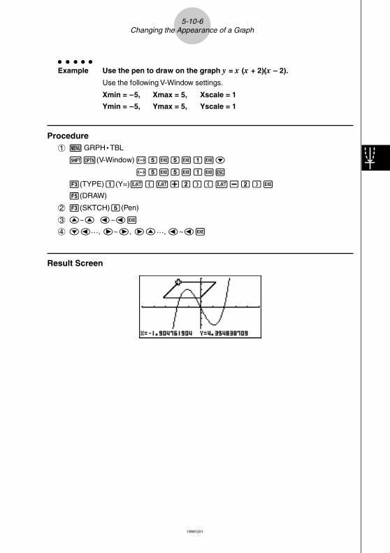
Example Use the pen to draw on the graph y = x (x + 2)(x – 2).
Use the following V-Window settings.
Xmin = –5, Xmax = 5, Xscale = 1
Ymin = –5, Ymax = 5, Yscale = 1
Procedure1m GRPH • TBL
!K(V-Window)-fwfwbwc
-fwfwbwi
3(TYPE)b(Y=)v(v+c)(v-c)w
5(DRAW)
23(SKTCH)f(Pen)
3f~f d~dw
4cd…, e~e, ef…, d~dw
Result Screen
5-10-6Changing the Appearance of a Graph
19991201

19990401
5-10-7Changing the Appearance of a Graph
kkkkk Changing the Graph Background
You can use the set up screen to specify the memory contents of any picture memory area(Pict 1 through Pict 20) as the Background item. When you do, the contents of thecorresponding memory area is used as the background of the graph screen.
○ ○ ○ ○ ○
Example 1 With the circle graph X2 + Y2 = 1 as the background, use DynamicGraph to graph Y = X2 + A as variable A changes value from –1 to 1 inincrements of 1.
Recall the background graph.
(X2 + Y2 = 1)

19990401
5-10-8Changing the Appearance of a Graph
Draw the dynamic graph.
(Y = X2 – 1)
↓↑(Y = X2)
↓↑(Y = X2 + 1)
• See “5-8-1 Dynamic Graphing” for details on using the Dynamic Graph feature.
19990401
5-11 Function Analysis
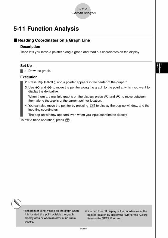
kkkkk Reading Coordinates on a Graph Line
DescriptionTrace lets you move a pointer along a graph and read out coordinates on the display.
Set Up1. Draw the graph.
Execution2. Press 1(TRACE), and a pointer appears in the center of the graph.*1
3. Use d and e to move the pointer along the graph to the point at which you want todisplay the derivative.
When there are multiple graphs on the display, press f and c to move betweenthem along the x-axis of the current pointer location.
4. You can also move the pointer by pressing v to display the pop-up window, and theninputting coordinates.
The pop-up window appears even when you input coordinates directly.
To exit a trace operation, press i.
*1The pointer is not visible on the graph whenit is located at a point outside the graphdisplay area or when an error of no valueoccurs.
# You can turn off display of the coordinates at thepointer location by specifying “Off” for the “Coord”item on the SET UP screen.
19991201
5-11-1Function Analysis
20011101

19990401
○ ○ ○ ○ ○
Example Read coordinates along the graph of the function shown below.Y1 = x2 – 3
Use the following V-Window settings.
Xmin = –5, Xmax = 5, Xscale = 1
Ymin = –10, Ymax = 10, Yscale = 2
Procedure1m GRPH • TBL
!K(V-Window)-fwfwbwc
-bawbawcwi
3(TYPE)b(Y=)vx-dw
5(DRAW)
21(TRACE)
3d~d
4-bw
Result Screen
5-11-2Function Analysis
# The following shows how coordinates aredisplayed for each function type.
• Polar Coordinate Graph
• Parametric Graph
• Inequality Graph
19991201
19990401
kkkkk Displaying the Derivative
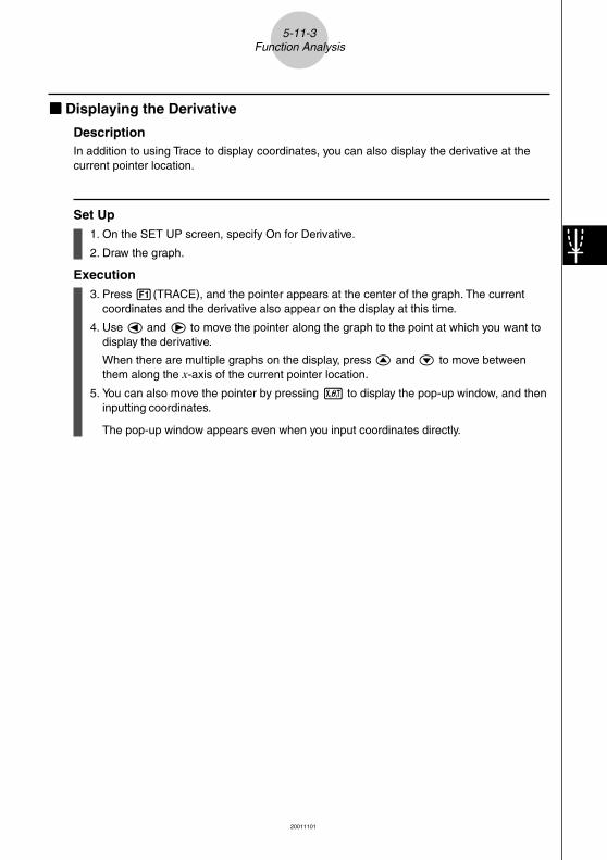
DescriptionIn addition to using Trace to display coordinates, you can also display the derivative at thecurrent pointer location.
Set Up1. On the SET UP screen, specify On for Derivative.
2. Draw the graph.
Execution3. Press 1(TRACE), and the pointer appears at the center of the graph. The current
coordinates and the derivative also appear on the display at this time.
4. Use d and e to move the pointer along the graph to the point at which you want todisplay the derivative.
When there are multiple graphs on the display, press f and c to move betweenthem along the x-axis of the current pointer location.
5. You can also move the pointer by pressing v to display the pop-up window, and theninputting coordinates.
The pop-up window appears even when you input coordinates directly.
5-11-3Function Analysis
20011101
19990401
○ ○ ○ ○ ○
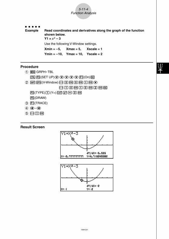
Example Read coordinates and derivatives along the graph of the functionshown below.Y1 = x2 – 3
Use the following V-Window settings.
Xmin = –5, Xmax = 5, Xscale = 1
Ymin = –10, Ymax = 10, Yscale = 2
Procedure1m GRPH • TBL
u3(SET UP)ccccc1(On)i
2!K(V-Window)-fwfwbwc
-bawbawcwi
3(TYPE)b(Y=)vx-dw
5(DRAW)
31(TRACE)
4d~d
5-bw
Result Screen
5-11-4Function Analysis
19991201

19990401
kkkkkGraph to Table
DescriptionYou can use trace to read the coordinates of a graph and store them in a number table. Youcan also use Dual Graph to simultaneously store the graph and number table, making this animportant graph analysis tool.
Set Up1. From the Main Menu, enter the GRPH • TBL Mode.
2. On the SET UP screen, specify GtoT for Dual Screen.
3. Make V-Window settings.
Execution4. Save the function and draw the graph on the active (left) screen.
5. Activate Trace. When there are multiple graphs on the display, press f and c toselect the graph you want.
6. Use d to move the pointer and press w to store coordinates into the number table.Repeat this step to store as many values as you want.
7. Press 6(CHNG) to switch the number table side.
8. From the pop-up window, input the list number you want to save.
5-11-5Function Analysis
19990401
○ ○ ○ ○ ○
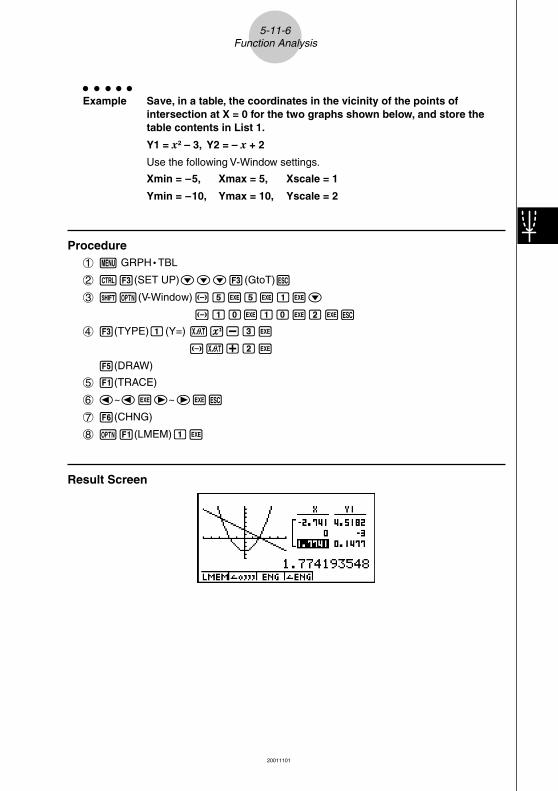
Example Save, in a table, the coordinates in the vicinity of the points ofintersection at X = 0 for the two graphs shown below, and store thetable contents in List 1.
Y1 = x2 – 3, Y2 = – x + 2
Use the following V-Window settings.
Xmin = –5, Xmax = 5, Xscale = 1
Ymin = –10, Ymax = 10, Yscale = 2
Procedure1m GRPH • TBL
2u3(SET UP)ccc3(GtoT)i
3!K(V-Window)-fwfwbwc
-bawbawcwi
43(TYPE)b(Y=)vx-dw
-v+cw
5(DRAW)
51(TRACE)
6d~dwe~ewi
76(CHNG)
8K1(LMEM)bw
Result Screen
5-11-6Function Analysis
20011101

19990401
kkkkk Coordinate Rounding
DescriptionThis function rounds off coordinate values displayed by Trace.
Set Up1. Draw the graph.
Execution2. Press 2(ZOOM)i(Rnd). This causes the V-Window settings to be changed
automatically in accordance with the Rnd value.
3. Press 1(TRACE), and then use the cursor keys to move the pointer along the graph.The coordinates that now appear are rounded.
5-11-7Function Analysis

19990401
○ ○ ○ ○ ○
Example Use coordinate rounding and display the coordinates in the vicinity ofthe points of intersection for the two graphs produced by thefunctions shown below.Y1 = x2 – 3, Y2 = – x + 2
Use the following V-Window settings.
Xmin = –5, Xmax = 5, Xscale = 1
Ymin = –10, Ymax = 10, Yscale = 2
Procedure1m GRPH • TBL
!K(V-Window)-fwfwbwc
-bawbawcwi
3(TYPE)b(Y=)vx-dw
-v+cw
5(DRAW)
22(ZOOM)i(Rnd)
31(TRACE)
d~d
Result Screen
5-11-8Function Analysis

19990401
kkkkk Calculating the Root
DescriptionThis feature provides a number of different methods for analyzing graphs.
Set Up1. Draw the graphs.
Execution2. Select the analysis function.
4(G-SLV)b(Root) ... Calculation of root
c(Max) ... Local maximum value
d(Min) ... Local minimum value
e(Y-lcpt) ... y-intercept
f(Isect) ... Intersection of two graphs
g(Y-Cal) ... y-coordinate for given x-coordinate
h(X-Cal) ... x-coordinate for given y-coordinate
i(∫dx) ... Integral value for a given range
3. When there are multiple graphs on the screen, the selection cursor (k) is located atthe lowest numbered graph. Use the cursor keys to move the cursor to the graph youwant to select.
4. Press w to select the graph where the cursor is located and display the valueproduced by the analysis.When an analysis produces multiple values, press e to calculate the next value.Pressing d returns to the previous value.
5-11-9Function Analysis
20011101
19990401
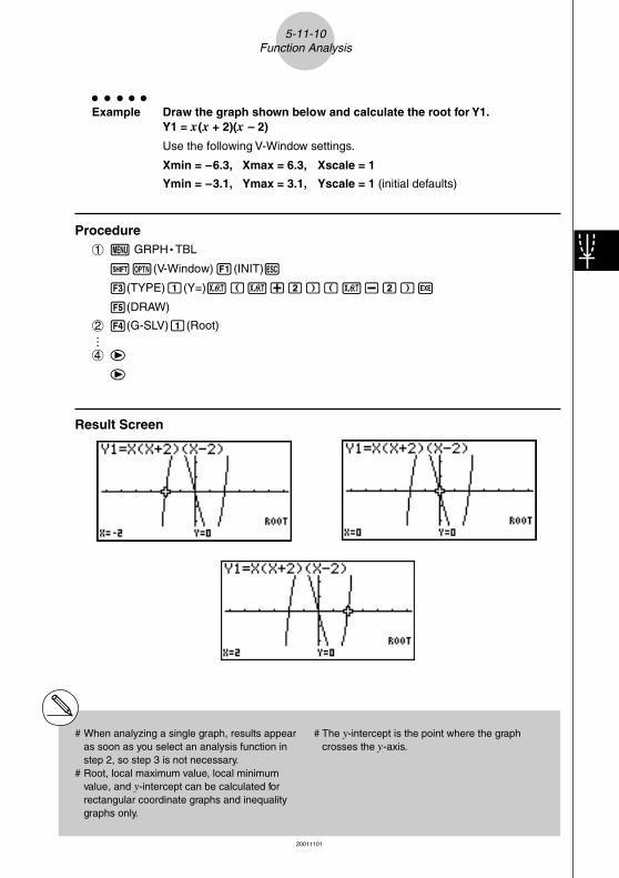
○ ○ ○ ○ ○
Example Draw the graph shown below and calculate the root for Y1.Y1 = x(x + 2)(x – 2)
Use the following V-Window settings.
Xmin = –6.3, Xmax = 6.3, Xscale = 1
Ymin = –3.1, Ymax = 3.1, Yscale = 1 (initial defaults)
Procedure1m GRPH • TBL
!K(V-Window)1(INIT)i
3(TYPE)b(Y=)v(v+c)(v-c)w
5(DRAW)
24(G-SLV)b(Root)
4e
e
Result Screen
5-11-10Function Analysis
# When analyzing a single graph, results appearas soon as you select an analysis function instep 2, so step 3 is not necessary.
# Root, local maximum value, local minimumvalue, and y-intercept can be calculated forrectangular coordinate graphs and inequalitygraphs only.
# The y-intercept is the point where the graphcrosses the y-axis.
…
20011101

19990401
kkkkk Calculating the Point of Intersection of Two Graphs
DescriptionUse the following procedure to calculate the point of intersection of two graphs.
Set Up1. Draw the graphs.
Execution2. Press 4(G-SLV)5(Isect). When there are three or more graphs, the selection cursor
(k) appears at the lowest numbered graph.
3. Use the cursor keys to move the cursor to the graph you want to select.
4. Press w to select the first graph, which changes the shape of the cursor from k to�.
5. Use the cursor keys to move the cursor to the second graph.
6. Press w to calculate the point of intersection for the two graphs.When an analysis produces multiple values, press e to calculate the next value.Pressing d returns to the previous value.
5-11-11Function Analysis

19990401
○ ○ ○ ○ ○
Example Graph the two functions shown below, and determine the point ofintersection between Y1 and Y2.Y1 = x + 1, Y2 = x2
Use the following V-Window settings.
Xmin = –5, Xmax = 5, Xscale = 1
Ymin = –5, Ymax = 5, Yscale = 1
Procedure1m GRPH • TBL
!K(V-Window)-fwfwbwc
-fwfwbwi
3(TYPE)b(Y=)v+bw
vxw
5(DRAW)
24(G-SLV)f(Isect)
6e
Result Screen
5-11-12Function Analysis
# In the case of two graphs, the point ofintersection is calculated immediately after youpress 4f in step 2.
# You can calculate the point of intersection forrectangular coordinate graphs and inequalitygraphs only.
…

19990401
k Determining the Coordinates for Given Points
DescriptionThe following procedure describes how to determine the y-coordinate for a given x, and thex-coordinate for a given y.
Set Up1. Draw the graph.
Execution2. Select the function you want to perform. When there are multiple graphs, the selection
cursor (k) appears at the lowest numbered graph.
4(G-SLV)g(Y-Cal) ... y-coordinate for given x
h(X-Cal) ... x-coordinate for given y
3. Use fc to move the cursor (k) to the graph you want, and then press w to selectit.
4. Input the given x-coordinate value or y-coordinate value.Press w to calculate the corresponding y-coordinate value or x-coordinate value.
5-11-13Function Analysis

19990401
○ ○ ○ ○ ○
Example Graph the two functions shown below and then determine the y-coordinate for x = 0.5 and the x-coordinate for y = 2.2 on graph Y2.Y1 = x + 1, Y2 = x(x + 2)(x – 2)
Use the following V-Window settings.
Xmin = –6.3, Xmax = 6.3, Xscale = 1
Ymin = –3.1, Ymax = 3.1, Yscale = 1 (initial defaults)
Procedure1m GRPH • TBL
!K(V-Window)1(INIT)i
3(TYPE)b(Y=)v+bw
v(v+c)(v-c)w
5(DRAW)
24(G-SLV)g(Y-Cal) 2 4(G-SLV)h(X-Cal)
3cw 3 cw
4 a.fw 4 c.cw
Result Screen
5-11-14Function Analysis
# When there are multiple results for the aboveprocedure, press e to calculate the nextvalue. Pressing d returns to the previousvalue.
# Step 3 of the above procedure is skippedwhen there is only one graph on the display.
# The X-Cal value cannot be obtained for aparametric function graph.
# After obtaining coordinates with the aboveprocedure, you can input different coordinatesby first pressing v.
19990401
kkkkk Calculating the lntegral Value for a Given Range
DescriptionUse the following procedure to obtain integration values for a given range.
Set Up1. Draw the graph.
Execution2. Press 4(G-SLV)i(∫dx). When there are multiple graphs, this causes the selection
cursor (k) to appear at the lowest numbered graph.
3. Use fc to move the cursor (k) to the graph you want, and then press w to selectit.
4. Use d to move the lower limit pointer to the location you want, and then press w.
You can also move the pointer by pressing v to display the pop-up window, and theninputting coordinates.
5. Use e to move the upper limit pointer to the location you want.
You can also move the pointer by pressing v to display the pop-up window, and theninputting the upper limit and lower limit values for the integration range.
6. Press w to calculate the integral value.
5-11-15Function Analysis
# You can also specify the lower limit and upperlimit by inputting them on the 10-key pad.
# When setting the range, make sure that the lowerlimit is less than the upper limit.
# Integral values can be calculated for rectangularcoordinate graphs only.
19991201

19990401
○ ○ ○ ○ ○
Example Graph the function shown below, and then determine the integral valueat (–2, 0).Y1 = x(x + 2)(x – 2)
Use the following V-Window settings.
Xmin = –6.3, Xmax = 6.3, Xscale = 1
Ymin = –4, Ymax = 4, Yscale = 1
Procedure1m GRPH • TBL
!K(V-Window)-g.dwg.dwbwc
-ewewbwi
3(TYPE)b(Y=)v(v+c)(v-c)w
5(DRAW)
24(G-SLV)i(∫dx)
4d~dw
5e~e(Upper limit; x = 0)
6w
Result Screen
5-11-16Function Analysis
…

19990401
kkkkk Conic Section Graph Analysis
You can determine approximations of the following analytical results using conic sectiongraphs.
• Focus/vertex/eccentricity
• Latus rectum
• Center/radius
• x-/y-intercept
• Directrix/axis of symmetry drawing and analysis
• Asymptote drawing and analysis
After graphing a conic section, press 4(G-SLV) to display the following graph analysismenus.
u Parabolic Graph Analysis• {Focus}/{Vertex}/{Length}/{e} ... {focus}/{vertex}/{latus rectum}/{eccentricity}
• {Dirtrx}/{Sym} ... {directrix}/{axis of symmetry}
• {X-Icpt}/{Y-Icpt} ... {x-intercept}/{y-intercept}
u Circular Graph Analysis• {Center}/{Radius} ... {center}/{radius}
• {X-Icpt}/{Y-Icpt} ... {x-intercept}/{y-intercept}
u Elliptical Graph Analysis• {Focus}/{Vertex}/{Center}/{e} ... {focus}/{vertex}/{center}/{eccentricity}
• {X-Icpt}/{Y-Icpt} ... {x-intercept}/{y-intercept}
u Hyperbolic Graph Analysis• {Focus}/{Vertex}/{Center}/{e} ... {focus}/{vertex}/{center}/{eccentricity}
• {Asympt} ... {asymptote}
• {X-Icpt}/{Y-Icpt} ... {x-intercept}/{y-intercept}
The following examples show how to use the above menus with various types of conicsection graphs.
5-11-17Function Analysis
20011101

19990401
u To calculate the focus, vertex and latus rectum[G-SLV]-[Focus]/[Vertex]/[Length]
○ ○ ○ ○ ○
Example To determine the focus, vertex and latus rectum for the parabolaX = (Y – 2)2 + 3
Use the following V-Window settings.
Xmin = –1, Xmax = 10, Xscale = 1
Ymin = –5, Ymax = 5, Yscale = 1
4(G-SLV)
b(Focus)
(Calculates the focus.)
i
4(G-SLV)
d(Vertex)
(Calculates the vertex.)
i
4(G-SLV)
f(Length)
(Calculates the latus rectum.)
• When calculating two foci for an ellipse or hyperbolic graph, press e to calculate thesecond focus. Pressing d returns to the first focus.
• When calculating two vertexes for an ellipse or hyperbolic graph, press e to calculatethe second vertex. Pressing d returns to the first vertex.
5-11-18Function Analysis

19990401
u To calculate the center and radius [G-SLV]-[Center]/[Radius]
○ ○ ○ ○ ○
Example To determine the center and radius for the circle(X + 2)2 + (Y + 1)2 = 22
Use the following V-Window settings.
Xmin = –6.3, Xmax = 6.3, Xscale = 1
Ymin = –3.1, Ymax = 3.1, Yscale = 1
4(G-SLV)
b(Center)
(Calculates the center.)
i
4(G-SLV)
c(Radius)
(Calculates the radius.)
u To calculate the x- and y-intercepts [G-SLV]-[X-Icpt]/[Y-Icpt]
○ ○ ○ ○ ○
Example To determine the x- and y-intercepts for the hyperbola
(X – 3)2 (Y – 1)2
–––––––– – –––––––– = 122 22
Use the following V-Window settings.
Xmin = –4, Xmax = 8, Xscale = 1
Ymin = –5, Ymax = 5, Yscale = 1
4(G-SLV)
g(X-Icpt)
(Calculates the x-intercept.)
5-11-19Function Analysis

19990401
i
4(G-SLV)
h(Y-Icpt)
(Calculates the y-intercept.)
• Press e to calculate the second set of x-/y-intercepts. Pressing d returns to the firstset of intercepts.
u To draw and analyze the axis of symmetry and directrix[G-SLV]-[Sym]/[Dirtrx]
○ ○ ○ ○ ○
Example To draw the axis of symmetry and directrix for the parabolaX = 2(Y – 1)2 + 1
Use the following V-Window settings.
Xmin = –6.3, Xmax = 6.3, Xscale = 1
Ymin = –3.1, Ymax = 3.1, Yscale = 1
4(G-SLV)
e(Sym)
(Draws the axis of symmetry.)
i
4(G-SLV)
c(Dirtrx)
(Draws the directrix.)
5-11-20Function Analysis

19990401
u To draw and analyze the asymptotes [G-SLV]-[Asympt]
○ ○ ○ ○ ○
Example To draw the asymptotes for the hyperbola
(X – 1)2 (Y – 1)2
–––––––– – –––––––– = 122 22
Use the following V-Window settings.
Xmin = –6.3, Xmax = 6.3, Xscale = 1
Ymin = –5, Ymax = 5, Yscale = 1
4(G-SLV)
e(Asympt)
(Draws the asymptotes.)
u To calculate eccentricity [G-SLV]-[e]
○ ○ ○ ○ ○
Example To determine the eccentricity of the graph for ellipse
(X – 2)2 +
(Y – 2)2 = 1
42 22
Use the following V-Window settings.
Xmin = –3, Xmax = 7, Xscale = 1
Ymin = –1, Ymax = 5, Yscale = 1
4(G-SLV)
e(e)
(Calculates eccentricity.)
5-11-21Function Analysis
# Certain V-Window parameters can produceerrors in values produced as graph analysisresults.
# The message ”Not Found” appears on thedisplay when graph analysis is unable toproduce a result.
# The following can result in inaccurate analysisresults or may even make it impossible to obtaina solution at all.— When the solution is tangent to the x-axis.— When the solution is a point of tangency
between two graphs.