MASSACHUSETTS GENERAL HOSPITAL

Granger Processing Stream

Manual for version 1.9

A. Conrad Nied, Bruna Olson, David Gow

2/12/2014

This document outlines the purpose and operation of the Graphical Processing Stream as produced by A. Conrad Nied in the lab of David W. Gow

GPS Manual 1 of 70

Contents

FORWARD

ACKNOWLEDGEMENTS AND OVERVIEW 5

Exhaustive Measurement 6

Non-redundancy 6

Stationarity 6

Proper Data 6

Goals 7

Citation 7

Licensing 7

CHAPTER 1: INTRODUCTION 8

Accessibility 8

Visualization 8

Reproducibility 8

CHAPTER 2: SETUP 9

Operating System 9

Software 9 Matlab 9 Freesurfer 9 Minimum Norm Estimates 9

Setup Routine 10

Graphical Processing Stream 11 Acquiring GPS 11 First Time Initialization 11 Starting it up 11 Organization 12

CHAPTER 3: ANALYSIS INTERFACE 13

Selecting Datasets 13

GPS Manual 2 of 70

Conditions 14 Further Specification 15

Stages and Functions 15

Status and Override 16

Batch 16

Function Management 16 Analysis Function Layout 17

Utilities 18

CHAPTER 4: ANALYSIS ROUTINES 21

4.1 Magnetic Resonance Imaging 21 4.1.1 Import 21 4.1.2 Finding the T1 MPRAGE file 21 4.1.3-5 Freesurfer Automatic Reconstruction 22 4.1.6-9 MNE Preparation 22 4.1.10 Converting the surfaces into a Matlab format 22 4.1.11 Average Brain Surface 22

4.2 Magnetoencephalography 23 4.2.1 Importing the Scan 23 4.2.2&3 Extracting and Processing Events 23 4.2.4 Bad Channels 23 4.2.5 Correcting for Blink and Eye Movement Artifacts 24 4.2.6 Coregistration 27

4.3 Minimum Norm Estimates 33 4.3.1 Averaging Sensor Data 33 4.3.2&3 MNE Forward and Inverse Solution 33 4.3.4 Extract Evoked Trials 33 4.3.5-7 Source Timecourses and Average Cortex Maps 34

4.4 Phase Locking Values 35 4.4.1 Region of Interest 35 4.4.2 & 3 Acquiring Trial Data for PLV Analysis 36 4.4.4 Computing Phase Locking 36 4.4.5-6 Average Brain Timecourses 36

4.5 Granger Causality 37 4.5.1&2 Regions of Interest 37 4.5.3&4 Gather Timecourses 38 4.5.6 Computing Granger-Causality using Kalman Filters 39 4.5.7 Generating Null Hypotheses to measure significance 39 4.5.8 Get Significance 39

CHAPTER 5: STRUCTURE EDITING INTERFACE 40

GPS Manual 3 of 70

Selection 40

Options 40

Saving 40

CHAPTER 6: REGION OF INTEREST INTERFACE 41

Organization 41

Loading Data 41

Brain Viewing Options 42 Surface 42 Viewing Angle 42 Background Overlays 43

Metrics 43 Five Measures of Source Activity 43 Time Window 44 Standardizing 44 Visualizing 44

Centroids 45

Creating Regions 47 Parameters 47 The Similarity Metric 48

Procedure 49

CHAPTER 7: PLOT DRAWING INTERFACE 50

Loading a Dataset 51

Rendered “Surface” Plots 53 Options 53

Cortical Activity 55

Regions, selection and labels 56

Granger Process 56 Methodology 57 Time 58

Granger Visualizations 58 Arrows 59 Nodes, “Bubbles” 60 Time Courses 61

GPS Manual 4 of 70

APPENDIX 1: REMOTE CONNECTING 64

Secure Shell (SSH) 64 Windows 64 Macintosh and Linux 65

Virtual Network Computing (VNC) 65 Windows 65 Macintosh 66

File Transfer Protocol (FTP) – Windows 67

APPENDIX 2: PARAMETERS 68

Common Parameters 68

Study 68

Subject 69

Condition 70

GPS Manual 5 of 70

Acknowledgements and Overview

The Granger Processing Stream (GPS) was developed by the Gow Group in the Department of

Neurology at the Massachusetts General Hospital and the Athinoula A. Martinos Center for

Biomedical Imaging with support from the National Institute of Deafness and Communicative

Disorders (R01 DC003108). It also benefited from the support of the MIND Institute and a

NCRR Regional Resource Grant (41RR14075) for the development of technology and analysis

tools at the Martinos Center. Many people contributed to the development of this stream

including David Gow, Jennifer Segawa, Ricky Sachdeva, Corey Keller, Mark Vangel, Reid

Vancelette, Bruna Olson, David Caplan and Seppo Ahlfors. Conrad Nied made invaluable

contributions to the approach, and is responsible for coding and developing GPS’s graphic user

interface and for writing most of this manual.

We developed it to address some of the inherent inferential limitations of behavioral and BOLD

imaging techniques. Our goal was to develop an analysis stream that respects the logic and

assumptions of Granger causality analysis. Our approach and its motivation is outlined at more

length in Gow & Caplan (2012). Granger analysis is built on an inference explored by Norbert

Wiener (1956) and later made practical by Clive Granger (1969) that causes both precede and

uniquely predict their own effects. The mathematical logic is simple. To understand what drives

a target signal (e.g. activation timecourse for some brain region), one can measure all non-

redundant, potentially causal signals and apply them to develop a mathematical prediction about

the future course of that signal. This prediction will inevitably be wrong. Mathematical models

quantify just how wrong it is using an error term. In Granger analysis, this prediction process is

then repeated using all measured signals except one. This will produce another error term. The

eliminated signal is said to Granger cause the predicted signal if dropping it from the prediction

causes a meaningful increase in the error term.

Granger analysis and its practical implementation rests on four main assumptions. These are all

directly addressed in GPS. They are:

GPS Manual 6 of 70

Exhaustive Measurement

In its strongest form, Granger analysis requires the measurement of all signals. If all signals are

measured and applied to prediction Granger analysis should be immune to spurious causation

artifacts. This assumption is unrealistic in virtually all applications of Granger analysis (and is

essentially ignored in bivariate approaches). Recognizing the limits of neuroimaging data, and

the practical consequences of applying factoral analysis to very large data sets, we developed

several automated approaches to ROI selection that allow the user to identify a set of candidate

ROIs based on changed activation relative to pre-trial baseline measures. Using our standard

parameter settings we typically perform analyses over networks comprised of 15 – 35 ROIs.

Users have the freedom to vary these parameters to produce more or less exhaustive sets, but

should recognize that the use of smaller sets may expose users to an increased risk of spurious

causation.

Non-redundancy

If two or more signals are identical (carry the same information), the logic fails because

removing one will result in no net loss of information. We address this assumption through an

automated ROI selection algorithm that limits the similarity between redundant ROIs. When two

signals are too similar, the candidate ROI with the strongest activation is typically retained.

Stationarity

In its original mathematical formulation, Granger analysis also assumes that all signals are

stationary (show no change in variance or central tendency over the time that is modeled). Neural

signals, and especially event-related neural activity is inherently non-stationary, and so this

assumption creates significant challenges when Granger analysis is applied these data. We

address this assumption through the use of time-varying multivariate autogression modeling

techniques. Because these approaches create a new model at each timepoint, there is no need to

assume stationarity. We rely on a Kalman filter technique developed by Milde et al. (2010) for

all analyses. One of the bonuses of this approach is that it makes it possible to quantify the

strength of Granger causation effects independently at each timepoint.

Proper Data

GPS relies on MR-constrained source space reconstructions of MEG/EEG activity over all

cortical surfaces. We do this for several reasons. From a mathematical standpoint, the timeseries

analyses needed to perform predictive modeling require a large number of datapoints. Kalman

filter techniques were developed (also with significant input from Norbert Wiener) for the

analysis of systems of noisy data and operate through an iterative process of prediction and

correction. When first applied, Kalman filters require some period of time to settle before they

provide reliably strong prediction. As a rule of thumb this process may require at least 100

timepoints. From a neuroscience perspective, the purpose of these analyses is typically to track

events that may take place over the order of tens of milliseconds. For these reasons, it is essential

to apply these analyses to high temporal resolution data (e.g. MEG/EEG). We do not recommend

the application of GPS to lower temporal resolution measures (e.g. BOLD signal). For the

purposes of interpretation, it is also essential to observe as much of the brain as possible (to

GPS Manual 7 of 70

identify all potentially causal signals) and to be able to relate activity to interpretable localized

processors. MR-constrained MEG/EEGG data support reconstructions over all cortical surfaces,

and provide spatial resolution that typically places sources within the range of a typical

Brodmann unit. Advances in multimodal imaging should improve this spatial resolution over

time, but at present the resolution is sufficient to relate measures of effective connectivity to

analyses of functional localization based on BOLD imaging and the analysis of the effects of

localized pathology.

Goals

Given appropriate funding, we hope to continue to develop and refine GPS. We are not currently

able to provide full support. For now, we hope to help identify a community of users who can

trade expertise. If you use GPS please let us know (gow@helix.mgh.harvard.edu).

Citation

For the time being, all citations of GPS should cite this manual, and the overview of our

approach provided in:

Gow, D.W., & Caplan, D. (2012). New levels of language processing complexity and organization revealed by Granger causation. Frontiers in Psychology, 3, 506. doi: 10.3389/fpsyg.2012.00506

The Kalman filter technique we use comes from: Milde, T., Leistritz, L., Astolfi, l., Miltner, W.H.G., Weiss, T., Babiloni, F., & Witte, H.

(2010). A new Kalman filter approach for the estimation of high-dimensional time variant multivariate AR models and its application in analysis of laser-evoked brain potentials. NeuroImage, 50, 960-969. Doi: 10.1016/j_neuroimage_2009.12.110.

Licensing

GPS is a GUI-based program written by A. Conrad Nied based on analyses developed by David

Gow and members of his lab at the Massachusetts Hospital to automate MNE and FSL analyses

of MR-constrained MEG/EEG data and to perform Kalman filter based Granger analyses of

those data. Copyright © 2014. A. Conrad Nied and David Gow.

This program is free software: you can redistribute it and/or modify it under the terms of the

GNU General Public License as published by the Free Software Foundation, either version 3 of

the license or (at your option) any later version.

This program is distributed in the hope that it will be useful, but WITHOUT ANY

WARRANTY; without even the implied warrantee of MERCHANTABILITY or FITNESS FOR

GPS Manual 8 of 70

A PARTICULAR PURPOSE. See the GNU Gneral Public License for more details

(http://www.gnu.org/licenses/).

Chapter 1: Introduction

The Matlab program suite was originally made to simplify the analysis process. As more routines

were incorporated the program grew and more user interfaces were added to the library. The

software contains many functions contributed to by many other researchers at the Athinoula A.

Martinos Center for Biomedical Imaging.

There are 3 design principles in the formation of this program suite: Accessibility, Visualization,

and Reproducibility.

Accessibility

All researchers regardless of specific programming background should be able to analyze their

data using software routines. By creating an interactive, visual environment, more people are

able to engage in the science.

Visualization

Data, not just the final result,should be easily visualized . At the end of the an analysis, the final

result may look defensible, but problems in middle steps can invalidate results. Thereby, instead

of operating routines as black boxes, GPS aims to provide visual feedback for each stage of the

result.

Furthermore, GPS provides and links to many interactive environments in which one can explore

their data and check for consistency.

Reproducibility

Due to the complex nature of brain imaging research, variance can be introduced at many stages.

Variance can be caused by subjects and experimental paradigms, but also small changes in

conducting an analysis, such as changing which channels to exclude for a subject or selecting

regions of interest that are a little off between subjects. After so many transformations of the

data, deviations in protocol can drastically change the final result.

Thereby, by providing a framework to organize a study and a system that is as automated as

possible, a stable protocol can be followed good results can be attained .

GPS Manual 9 of 70

Chapter 2: Setup

Operating System

The interface is compatible with Mac OS X and Linux. However, it was built on a Linux

machine (Cent OS) and is thereby optimized for operation on Linux. Some computer

configurations may case graphical glitches with the Matlab graphical user interface (GUI)

routines. These mostly affect the alignment of certain interface elements but it will not affect the

data.

Software

Three programs are necessary in order to run the Graphical Processing Stream. Martinos Center

users already have this software provided.

Matlab

The processing stream is run out of Matlab. Additionally, it uses a number of Matlab toolboxes,

packages of functions necessary for the interface. Some of the toolboxes may need to be acquired

separately. In order to run all aspects of the processing stream one will need:

Matlab 7.11 or later and necessary toolboxes:

o Image Processing Toolbox

o Distributed Computing Toolbox

o Statistics Toolbox

http://www.mathworks.com/products/matlab/

Freesurfer

This program is used to process Magnetic Resonance Imaging (MRI) scans. It reconstructs

cortical surfaces from raw brain images. The analysis stage called MRI (in Chapter 5.2) utilizes

many Freesurfer commands. Freesurfer is crucial for GPS to use the Minimum Norm Estimates

toolbox in constructing cortical and skull maps. See the websites for more information:

Main portal: http://surfer.nmr.mgh.harvard.edu/

Download: http://surfer.nmr.mgh.harvard.edu/fswiki/DownloadAndInstall

Additional Freesurfer Matlab functions are bundled with the GPS routines. These commands

import the Freesurfer data in order to render images of the brain.

Minimum Norm Estimates

Matti Hämäläinen’s Minimum Norm Estimates software creates estimates of cortical activity by

combining Freesurfer cortical surfaces with MEG/EEG signals. GPS started as shell program,

interacting with the MNE routines. At their current state, most functions in GPS are independent

of MNE but MNE was instrumental in designing the functions.

GPS Manual 10 of 70

http://www.martinos.org/mne/

Setup Routine

After these software packages have been installed and loaded into the environment, the

processing stream can be opened in Matlab. Setting up the environment can be done easily using

a tsch or bash script, such as the tsch script provided below. All phrases in ‘< >’ signs refer to

variables that should be indicated by the user.

# Set the folder where GPS is located setenv WORKHOME <GPS directory> cd $WORKHOME # Load the Freesurfer software setenv FREESURFER_HOME <Freesurfer directory> source $FREESURFER_HOME/SetUpFreeSurfer.sh setenv FSFAST_HOME $FREESURFER_HOME/fsfast setenv MNI_DIR $FREESURFER_HOME/mni # setenv FSL_DIR <FSL software directory> setenv SUBJECTS_DIR <Study processed MRI directory> # Load the Minimum Norm Estimate software setenv MNE_ROOT <MNE software directory> setenv MATLAB_ROOT <Matlab software directory> source $MNE_ROOT/bin/mne_setup # Start Matlab matlab

For the users in the Martinos center in particular, use these commands:

# Set the folder where GPS is located setenv WORKHOME <GPS directory> cd $WORKHOME # Load the Freesurfer software source /usr/local/freesurfer/nmr-stable52-env setenv FSFAST_HOME /usr/local/freesurfer/stable4/fsfast setenv MNI_DIR /usr/local/freesurfer/stable4/mni setenv FSL_DIR /usr/pubsw/packages/fsl/current setenv SUBJECTS_DIR <Study processed MRI directory> # Load the Minimum Norm Estimate software setenv MNE_ROOT /usr/pubsw/packages/mne/nightly_build setenv MATLAB_ROOT /usr/pubsw/packages/matlab/current source $MNE_ROOT/bin/mne_setup # Start Matlab matlab8.0

GPS Manual 11 of 70

In order to speed up the execution of these commands, it is recommended to save these into a

shell file and create an alias for the command. For instance, if these commands are saved in the

file “setup_GPS” located in the home directory, users should edit the “.cshrc” (or .bashrc) file in

the home directory, by adding the line:

alias GPS course ~/setup_GPS

This will enable the user to load Matlab set with the environment for the graphical processing

stream by just typing the shell command “GPS”.

Graphical Processing Stream

A processing stream is a collection of programs organized into steps that perform an analysis.

The processing stream consists of four primary interface programs and a host of functions.

Acquiring GPS

GPS is hosted on Martinos Center website. You can download the repository from:

www.martinos.org/software/GPS

First Time Initialization

The first time you run GPS, you will need to run a script to initialize the functions. The script is

called gps_init.m and is located in the main directory. Run it out of Matlab. This function will

ask you which directory is GPS located in, and the desired locations for the images, logs, and

parameters files. It will optionally clear the parameters folder, so if you are starting over click

yes, otherwise click not to clear the parameters folder. Staring over will remove all images in the

images directory so make sure you have backed up any images.

Starting it up

After setting up the environment, the user interface can be started up by typing the command

GPS in Matlab. This command will add the GPS functions to the Matlab path and bring up a

dialogue for the user to choose which interface to open as seen in Figure 2.1. This menu can be

reopened at any time by typing GPS again.

GPS Manual 12 of 70

Organization

The GPS directory contains four folders and the starter GPS functions.

The functions folder contains all of the Matlab routines used by the GUIs and analysis. Images

made specific for Matlab sessions are put in the images folder. The image folder pictures are

organized by date. The logs folder contains records for the analysis routines for each study. The

parameters folder contains all of the analysis parameters such as timing and thresholds. These

parameters can be edited using the structure-editing interface as described in Chapter 6.

The scans, intermediate analyses and results for the studies are saved in a separate folder for the

study. Images that are permanent records for analysis are saved in the study folder, but

intermediate or interface-driven images are saved in the GPS/images folder (or other if you

specified).

Figure 2.1

GPS Manual 13 of 70

Chapter 3: Analysis Interface

For the sake of generalizing and accessibility, the analysis functions have been streamlined and

put in one interface.

Selecting Datasets

The top of the interfaces has three lists. The first list enables the user to select a study and then

the study’s subjects and conditions’ subsets can be modified. Once a study is selected, many

interior variables are changed and analysis functions may change. The new and edit buttons can

Figure 3.1

GPS Manual 14 of 70

be used to add new studies and open the structure editing interface to edit parameters of the study

selected.

Subjects and conditions are specified on the other two lists. Multiple items can be specified using

shift (for continuous selection) and ctrl (for discrete selection). The ‘All’ buttons under each list

will select all elements in that list. Every time the selection of the study, subject, or condition is

altered, the program will reload certain elements and refresh the status bars.

Conditions

An important design consideration is the organization of trials into sets. For instance, the

investigator may want to look at the data in one combination initially, but then combine or split

up the data later. Each relevant combination of data should be analyzed as a different condition.

Primary v Secondary Conditions One important distinction is the differentiation between primary and secondary conditions.

Certain analyses may call for straightforward divisions of the analysis, like all trials into sets A

and B. However, later analyses may ask to use only some of the trials from A or splitting it into

two more subsets C and D. Instead of locking the user into specific data conditions from the

start, the program is meant to be run first for initial subsets. These conditions should cover all of

the data, yet not overlap, because it is used in the construction of the map between cortical and

sensor activity. Secondary conditions can be additional sets derived from the primary sets or

novel combinations.

Figure 3.2

GPS Manual 15 of 70

Further Specification

The Settings button opens a menu, shown in figure 3.3 to enable further customization of the

dataset.

In large groups, the study list may get long so individual users can specify which studies they

would like to see in the main GUI through this dialogue. This list can be changed at any time,

just note that it will reinitialize the list of studies in the main window.

Stages and Functions

The lower half of the analysis interface is used to run the analysis functions. The left column lists

various stages of the analysis: Utilities, MEG, MRI, MNE, PLV, and Granger. They will be

detailed in Chapter 5. Clicking on one of these buttons will change the function list on the right

side to the list of functions for the particular analysis stage.

The functions show up as a series of buttons showing the progressive routines of the particular

stage. Clicking on a single button will start the analysis for the selected subject(s) and

condition(s). Some functions work across all subjects and/or all conditions.

Figure 3.3

GPS Manual 16 of 70

Status and Override

In each function script, there is a portion of the code dedicated to determine if a function is ready

to be performed and if it has been completed. The grey rectangles next to each stage and function

show its progress when the “Refresh Status” checkbox is checked at the bottom of the screen –

changing the selected subjects and conditions will cause the interface to recheck the existence of

files on the hard drives so it could take a few seconds to show the correct status.

For certain functions, the ready/finished status of routines is determined on demand when they

are called by the interface to be processed. If a function is not ready to be processed or it has

already finished and isn’t repeatable, it will not run. To rerun a finished function, check the

“Override” checkbox, sometimes this may require you to delete the already finished results but

that case should only happen with the Freesurfer commands. The table below shows the various

readiness statuses and their corresponding coloring

Batch

The checkboxes next to stage and function names are included to aid in the serial processing of

many functions. If multiple items in the function list are selected and the “Batch” button is

clicked, the program will attempt to do each function selected for each selected subject and

condition as necessary. If a process fails covertly it will detect the next function is not ready and

won’t proceed for that particular dataset (subject/condition). If a process bugs the interface it will

halt the execution.

Function Management

For the Analysis Interface, functions are organized by stages in their directories under

functions/gpsa/<stage>/… Instead of keeping a solid list of functions, in each stage directory

there is a program that returns the list of functions for that stage: there interface name and the

program name. This file can be amended to remove or add buttons to the particular stage in the

interface.

Functions can be edited for specific studies as well. For example, the event processing function

of the MEG stage is customized for each study. The GUI will automatically look for functions

that match the pattern <function>_<study.name>.m before it processes <function>.m

Most analysis functions are created with the framework on the following page Each function can

be run from the Matlab command line with the state specified –a structure containing the fields

Not Ready Partially

Ready

Ready Partial

Ready

Partial

Finish

Partially

Finished

Finished

Figure 3.4

GPS Manual 17 of 70

.study indicating the study name, .subject, and .condition, and also .dir specifying the GPS

folder.

Analysis Function Layout

function varargout = gpsa_<function name>(varargin)

% <function description>

%

% Author: <author>

%

% Changelog:

% <date> <edits>

%% Input

[state, operation] = gpsa_inputs(varargin);

%% Prepare a report on the type of the function

if(~isempty(strfind(operation, 't')))

report.spec_subj = <is the function subject specific?>;

report.spec_subs = <is the function condition specific?>;

end

%% Execute the process

% If it is proper to do the function

if(~isempty(strfind(operation, 'c')))

subject = gpsa_parameter(state, state.subject); % Get subject structure

state.function = 'gpsa_<function name>';

tbegin = tic;

<function contents>

% Add an entry to the log reflecting the processing of this function

gpsa_log(state, toc(tbegin));

end % If we should do the function

%% Add to the report concerning the progress

if(~isempty(strfind(operation, 'p')))

subject = gpsa_parameter(state, state.subject);

if(~isempty(subject))

% Predecessor: <function's predecessors>

report.ready = <ready logical statement>;

report.progress = <progress logical statement>;

report.finished = report.progress == 1;

else

report.ready = 0;

report.progress = 0;

report.finished = 0;

end

end

%% Prepare the report and output

if(nargout == 1 && exist('report', 'var'));

varargout{1} = report;

end

GPS Manual 18 of 70

end % function

Utilities

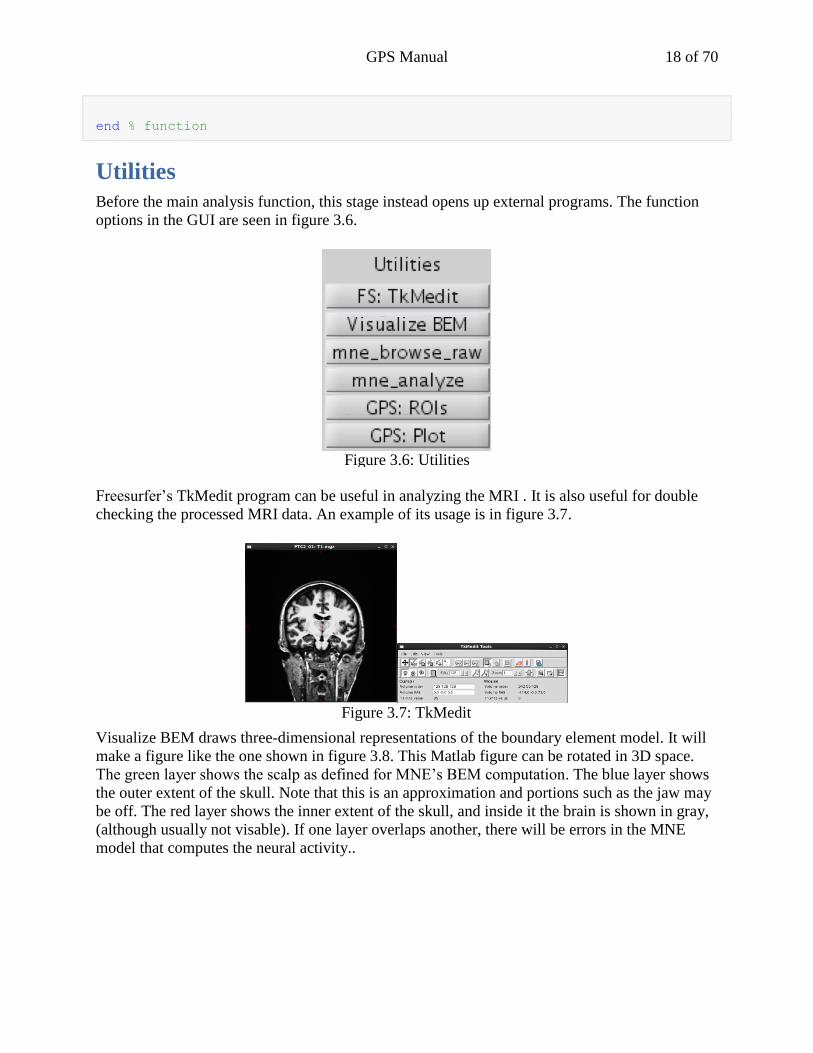
Before the main analysis function, this stage instead opens up external programs. The function

options in the GUI are seen in figure 3.6.

Freesurfer’s TkMedit program can be useful in analyzing the MRI . It is also useful for double

checking the processed MRI data. An example of its usage is in figure 3.7.

Visualize BEM draws three-dimensional representations of the boundary element model. It will

make a figure like the one shown in figure 3.8. This Matlab figure can be rotated in 3D space.

The green layer shows the scalp as defined for MNE’s BEM computation. The blue layer shows

the outer extent of the skull. Note that this is an approximation and portions such as the jaw may

be off. The red layer shows the inner extent of the skull, and inside it the brain is shown in gray,

(although usually not visable). If one layer overlaps another, there will be errors in the MNE

model that computes the neural activity..

Figure 3.6: Utilities

Figure 3.7: TkMedit

GPS Manual 19 of 70

Minimum Norm Estimate’s mne_browse_raw and mne_analyze programs help in preprocessing

and viewing the data after the estimates have been created. Their usage will be detailed in the

MNE section.

The remaining two buttons open up interfaces developed along with GPS.

GPS: ROIs is used to automatically cluster regions of the brain based on neural activity; it is

described in more detail in chapter 6.

GPS: Plot creates an environment to visualize granger causality, it is described in chapter 7.

Figure 3.8: Visualize BEM

Figure 3.9: mne_browse_raw

Figure 3.10: mne_analyze

GPS Manual 20 of 70

Figure 3.9: GPS ROIs

Figure 3.10: GPS Plot

GPS Manual 21 of 70

Chapter 4: Analysis Routines

4.1 Magnetic Resonance Imaging

The MRI stream is largely automated. It is broken down into sections based on the functions run.

Steps 2 to 9 are automated so they can be easily batch ran together.

4.1.1 Import

When this program is run, it will ask the user whether to retrieve the raw MRI scan from the

Bourget computer cluster or a specified location. If Bourget is selected, it will attempt to find the

location of the folder with the subject’s MRI on that server using the Martinos command

findsession. Otherwise, the user can retrieve an MRI scan from a specified folder – most

useful when importing from the compact disk drive. On most Linux machines, the CD drive is in

the folder /Media.

The raw MRI scan will be imported to <study.mri.rawdir>/<subject.name>

4.1.2 Finding the T1 MPRAGE file

The next program scans through the subject’s raw MRI directory to locate the T1 MPRAGE scan

file in order to process the Freesurfer reconstruction. This will use the Martinos center shell

command unpacksdcmdir. The program scans the unpack.log file for which file corresponds to

the entire – or start of – the T1 MPRAGE scan. There may be cases in which this function will

not work on the raw MRI data. If the file containing the T1 MPRAGE scan is known, that file

Figure 4.1: MRI Processing Functions

GPS Manual 22 of 70

can be manually selected using the Structure Editing Interface under the variable

subject.mri.first_mpragefile.

4.1.3-5 Freesurfer Automatic Reconstruction

The buttons Organize, Build Surfaces, and FS Average are all steps in the Freesurfer

reconstruction of the cortical surface. If any of these functions need to be redone, it may be

necessary to manually delete the subjects MRI directory in which it writes the file to. The default

folder for this is <study.mri.dir>/<subject.name>. These programs call on the three primary

sections of the recon-all command.

Organize (-autorecon1) extracts the important data from the T1 MPRAGE scan

Build Surfaces (-autorecon2) creates the white matter, grey matter, scalp, and many

other surfaces important for cortical processing

FS Average (-autorecon3) maps the subject’s brain to the Freesurfer average brain and

automatically parcellates the brain into regions.

4.1.6-9 MNE Preparation

The next few buttons call MNE commands in the shell through Matlab.

Source Space (mne_setup_source_space) creates a decimated vertex based

representation of the cortical surface based on the one made in Freesurfer,. It usually ends

up with 10,000 vertices in an effort to compress the data.

Setup Coreg (mne_setup_mri) creates the files necessary for the coregistration step

found in the MEG routines.

BE Model (mne_watershed_bem) constructs the Boundary Element Model used in the

source estimation process – particularly for the EEG signals. It also copies a few files to

folders for some of the other programs.

BE Model to .fif (mne_setup_forward_model) does the steps necessary to set up the

forward model.

4.1.10 Converting the surfaces into a Matlab format

In order to decrease the time it takes for the software to load subject’s brain data, this function

collects all the surfaces and some forward model elements into a Matlab matrix file. When doing

this for the last subject, it will automatically attempt to do this for the average subject brain.

4.1.11 Average Brain Surface

This function creates a brain using the Freesurfer command make_average_subject to combine

the brains of each of the subjects into an average one. Run this command after you have

processed the MRIs for all of the subjects in the study.

GPS Manual 23 of 70

4.2 Magnetoencephalography

This step prepares the data for the Minimum Norm Estimates analysis, and it requires the most

user input.

4.2.1 Importing the Scan

After completing the MEG scan that data will be ready to be imported using the Import button.

The system is configured to first look for the data on the Martinos network megraid server. The

program will ask for the number of the megraid hard drive that the data was saved to and save it

to the subject’s parameters as subject.meg.raid. It will look for the scan data under the folder:

/space/megraid/<subject.meg.raid>/MEG/<study.meg.raid_pi>/subj_<subject.name>

If it isn’t able to find the right files it will prompt the user to locate the correct directory

containing the MEG recordings.

4.2.2&3 Extracting and Processing Events

The Extract Events button will automatically extract the event information to .eve files into the

MEG/<subject.name>/triggers directory. Older versions of the MEG software recorded a

different event channel so the program will try both channels.

Processing events will require a customized program for each study. It will associate the events

recorded during the MEG recording with additional features defined by the user. It will create

event files with new event codes based on the primary conditions.

4.2.4 Bad Channels

The user must mark abnormal channels to prevent them from affecting the analysis later on.

Channels are usually bad when : 1) There is a large amplitude difference or 2) There is an

unusual periodic or random signal not found in other channels. It is often hard to determine

exactly if a channel is abnormal. EOG channels should not be marked in this fashion. The user

should load one or two blocks in mne_browse_raw and write down channels that are abnormal.

Then they should click on the button BadChannel and type the identified bad EEG and MEG

channels in their respective boxes. These channels will be ignored and not used in the analysis.

Figure 4.2: MEG Preprocessing Functions

GPS Manual 24 of 70

4.2.5 Correcting for Blink and Eye Movement Artifacts

Although there are many attested ways to mitigate the effects of eye blinks in brain signals, this

software is configured to use the principal component analysis implemented in MNE’s

mne_browse_raw program. In order to use this, the user must open a block of the MEG scan in

mne_browse_raw and select eye blinks by creating an additional event – conventionally number

555. Scroll through the vertical EOG data and mark the center of the blinks with the cursor then

click the “Picked to” button with the number 555. Note the duration of the blink artifacts.

Figure 4.3: mne_browse_raw showing a bad channel in black

Figure 4.4: The input dialog in GPS: Analysis marking

bad channels by channel number designation

GPS Manual 25 of 70

Click on the function Process/Create a new SSP Operator…. This command performs a

principal component analysis of the data, based on the time period selected. We will use this

analysis to identify the principal components related to blinking. The routine allows the user to

enter the start time and the end time of the subject’s blinks relative to the marks created for the

particular event number. For instance, in the data shown (see figure 4.6) the blinks are 400 ms

long and marked to the channel 555. If this process fails, it is likely because it was not able to

locate enough time samples in this window, so more blinks should be selected or there could be

another issue with the data.

Now, a menu of principal component analysis projections will appear. Multiplying the data by

these projections (vectors) should remove artifacts from the raw data. PCA decomposes

components that reflect the major underlying signals. The most prominent components will be

the blinks, but be very careful: auditory processing signals may also be detected by the data; if

they are screened out using the principal component analysis then the data is destroyed. Thereby,

the task is to identify the components that affect the data the most negatively and are correlated

with the eye blinks. The saved eye blink events will have light blue lines so the events can be

seen on the EEG and MEG channels. Select projections for the EEG channels, the MEG planar

gradiometers, and the MEG axial magnetometers. It is useful to find a page of channels that are

overtly influenced by the blinks to operate on.

Figure 4.5: mne_browse_raw showing the EOG channels with marked artefacts

Figure 4.6: Dialogue in mne_browse_raw prompting the user to select a time window

GPS Manual 26 of 70

Once the projections that clean up the blinks have been selected, select all the existing

projections. Before you save, make sure that the “Include EEG average reference” option has

been checked. Click accept and save the file as <subject.name>_eog_proj.fif in the subject’s

MEG raw data directory. As long as the analysis interface shows that you have the same eog

projection file it will automatically apply the EOG projections.

Figure 4.7: EEG channels with a blink before and after a successful projection

Figure 4.8: MEG channels with a blink before and after a successful projection. Note that the

non-blink related bump a few hundred milliseconds after the blink is preserved.

GPS Manual 27 of 70

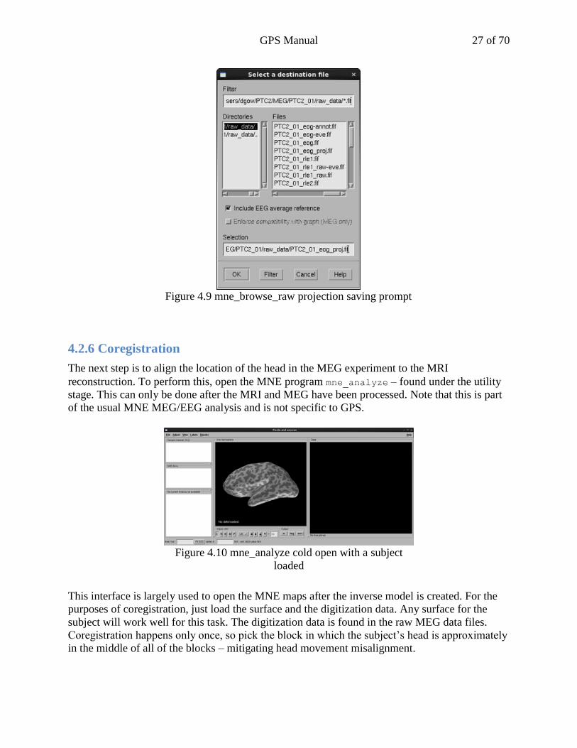
4.2.6 Coregistration

The next step is to align the location of the head in the MEG experiment to the MRI

reconstruction. To perform this, open the MNE program mne_analyze – found under the utility

stage. This can only be done after the MRI and MEG have been processed. Note that this is part

of the usual MNE MEG/EEG analysis and is not specific to GPS.

This interface is largely used to open the MNE maps after the inverse model is created. For the

purposes of coregistration, just load the surface and the digitization data. Any surface for the

subject will work well for this task. The digitization data is found in the raw MEG data files.

Coregistration happens only once, so pick the block in which the subject’s head is approximately

in the middle of all of the blocks – mitigating head movement misalignment.

Figure 4.9 mne_browse_raw projection saving prompt

Figure 4.10 mne_analyze cold open with a subject

loaded

GPS Manual 28 of 70

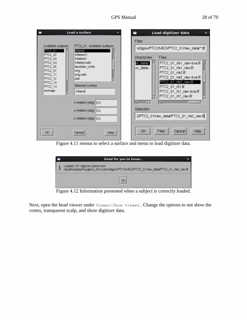
Next, open the head viewer under Viewer/Show viewer… Change the options to not show the

cortex, transparent scalp, and show digitizer data.

Figure 4.11 menus to select a surface and menu to load digitizer data.

Figure 4.12 Information presented when a subject is correctly loaded.

GPS Manual 29 of 70

Now, open the Coordinate alignment interface under the Adjust menu. The first task will be

to select the locations of the fiducials on the scalp. For each point, click each fiducial button (LAP

– Left Auricular Point, Nasion, RAP) in Figure 4.15 area 1, and then click the approximate

corresponding location for each point on the scalp.

Figure 4.13 MRI head surface viewer at load and after selecting the head coordinates

Figure 4.14 Viewer options to visualize head coordinates

GPS Manual 30 of 70

After the fiducials have been located, click Align using fiducials and it will align the EEG

points to the scalp. Each circle corresponds to each point clicked on by the digitizing pen. The

size of the circles reflects the distance from the MRI computed scalp. Blue circles represent

points inside the scalp and red circles represent points outside the scalp.

Figure 4.15 Coordinate alignment menu

Figure 4.16 Subject’s scalp surface with mouse cursor above the three

fiducials, from left to right: RAP, Nasion, LAP

GPS Manual 31 of 70

In order to refine the alignment, let the program automatically align the points to the best fit.

Under the ICP align option in area 2 (and see in figure 4.18), set it to 50 steps and click the

button. This will move the points to a better fit to the scalp.

Next, discard the points that are far away and are biasing the automatic alignment by omitting

points that are more than half a centimeter away. This button is found in area 3 of the coordinate

alignment interface. Then click the ICP align button again.

Save the coregistration using the Save MRI set button in area 4. It will save a file in the

subject’s MRI directory with the date and time of this coregistration.

Figure 4.17 Scalp surface in in three stages

1) After fiducial alignment

2) After automated ICP alignment

3) After discarding far points and additional ICP alignment

Figure 4.18 Automatic alignment box

Figure 4.19 Point discard selection box

GPS Manual 32 of 70

Back in the Analysis interface, click on the MEG/Coregistration button and select the file that

was just created in the mne_analyze interface.

Figure 4.20 Saving dialog

Figure 4.21 Selecting that saved file in the GPS Analysis prompt

GPS Manual 33 of 70

4.3 Minimum Norm Estimates

This stage of the analysis constructs a matrix that maps sensor activity to the cortical surface.

Each function is highly automated, therefore user should only split it into phases in case certain

stages need to be re-run.

4.3.1 Averaging Sensor Data

After the events have been processed, bad channels marked, and EOG projection made, the data

from the sensors can be averaged. Averaging the MEG and EEG waves will increase the signal

to noise ratio. This step will create .fif files containing the waves. It will first make files for

each block and then an average for the whole subject. This stage will also create averages for the

covariance processing in order to weigh down noisy channel data. It is important to be familiar

with the study.mne parameters and the condition.event parameters. Before processing this,

consult Appendix 2. This step will only create averages for conditions considered primary

conditions. This process filters out frequencies higher than 60 Hz from the sensor data. Filtered

block .fif files are saved in <subject.meg.dir>/processed_data/ and are used later in the

Granger analysis.

4.3.2&3 MNE Forward and Inverse Solution

These programs route information to the MNE routines that create a model mapping cortical

activity to sensor activity and then back around. There are particular options that can be changed

for this process if the Matlab code is modified.

4.3.4 Extract Evoked Trials

The next step is to gather the evoked trials into groups based on each event code set in the

Process Events step. It will make a series of .mat files with names based on the event codes that

can be collected later on for trial analysis.

Figure 4.21 MNE Processing Functions

GPS Manual 34 of 70

4.3.5-7 Source Timecourses and Average Cortex Maps

These functions make source timecourses, illustrating the activity on the cortical surface over

time. The Make .stc function creates stc files with the mne tag based on the sensor averages and

the inverse solution – only for the primary conditions. The Morphed .stc function will make stc

files on the average cortical surface It is done in the same manner as the primary conditions, but

it will also convert act tagged .stc files for secondary conditions made during the granger-

>condition phase. The Average Subject button will combine the morphed .stc files.

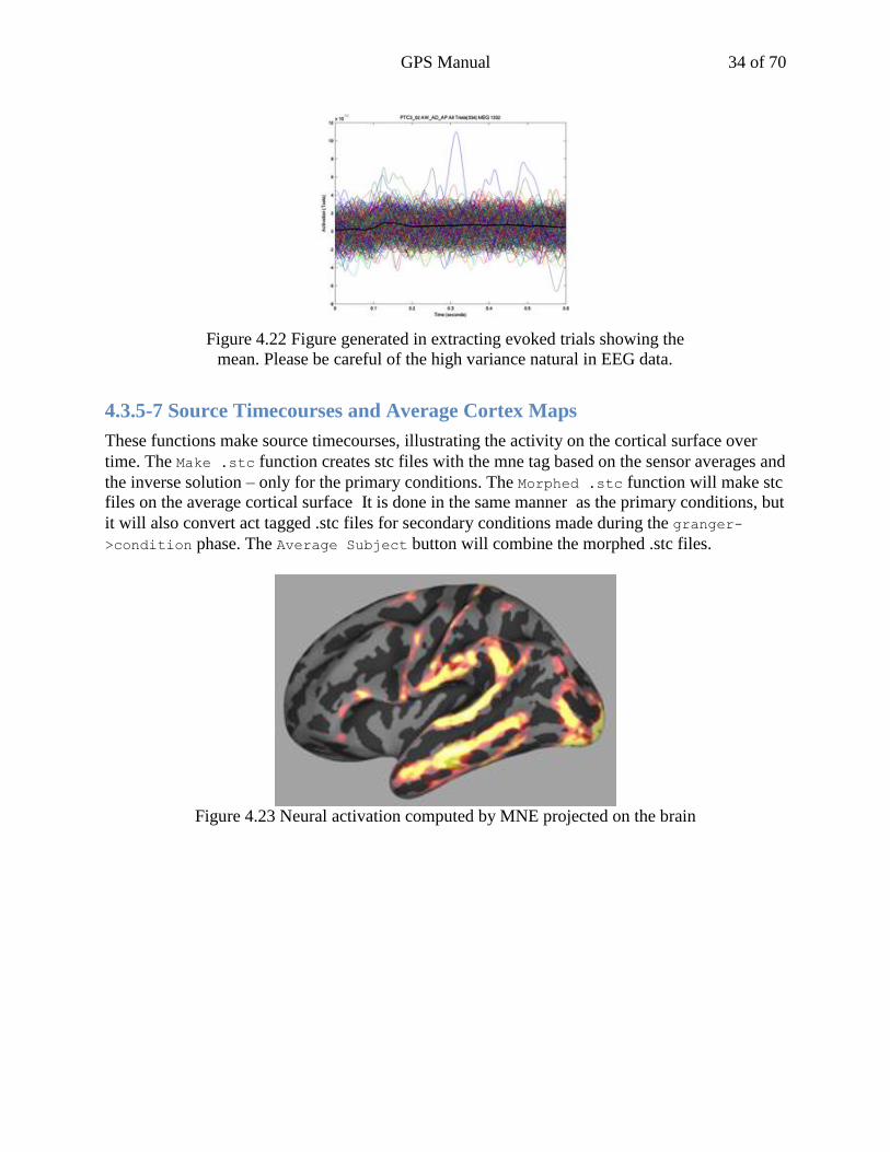
Figure 4.22 Figure generated in extracting evoked trials showing the

mean. Please be careful of the high variance natural in EEG data.

Figure 4.23 Neural activation computed by MNE projected on the brain

GPS Manual 35 of 70

4.4 Phase Locking Values

Please note that this function has been temporarily removed from the interface and will be

restored later when the group is satisfied with it. To restore the PLV stage, manually edit the

gps_presets.m file and add a stage called “plv” to the stages and stage_names fields. Additional

stages can also be added by editing this part. You will need to edit gpsa_load_stage.m for

additional stages

In order to better locate regions of interest, our lab sought to make use of metrics related to

functional connectivity. Phase locking values measure the similarity in the phase of two waves.

The technique takes a label for one region of interest and computes the phase locking between

that area and the rest of the brain, generating .stc files similar to the ones in the MNE stage.

4.4.1 Region of Interest

The program expects the user to create a region of interest .label file (either in mne_analyze or

in the ROI interface) and put it in the <study.plv.dir>/rois/<condition.name> folder. The

Reference ROIs button will map average subject labels to each individual subject. If multiple

labels are in that folder they will also be mapped, but usually only one reference ROI will be

used in the PLV analysis. The program will also create an image of the reference vertex on the

brain showing were the vertices were located with the cortical activation backdrop.

Figure 4.24 PLV Analysis functions

Figure 4.25 Neural Activation looked at to make a reference ROI

GPS Manual 36 of 70

4.4.2 & 3 Acquiring Trial Data for PLV Analysis

The next two buttons extract sensor data and put them into .mat files to be used in the Compute

PLV routine. Gather Trials gets evoked responses from the condition.event parameters.

Emptyroom Trials extracts chunks of time for simulated trials from the subjects emptyroom

file.

4.4.4 Computing Phase Locking

Functional connectivity analyses provide an obvious tool for identifying ROIs. We are extremely

interested in the use of ~40 Hz gamma phase locking meaures for this purpose. In theory, one

would identify a reference ROI and identify other ROIs based on phase locking with this signal.

This routine will generate .mat and .stc movies of the phase locking values on the subject’s

cortical surface. However, we caution against using them in their current form because these

analyses show a strong spatial bias to the region around the reference site.

4.4.5-6 Average Brain Timecourses

For group level analysis, the Morphed .stc button maps the subject’s phase locking .stc file to

the average brain. Average Subject will combine the morphed files to get a study-wide average

of phase locking.

Figure 4.26 Phase locking values to the STG mapped on to the cortex

GPS Manual 37 of 70

4.5 Granger Causality

The final stage of the MEG analysis is to compute the functional connectivity measured in

Granger causality created using Kalman filters.

4.5.1&2 Regions of Interest

To begin Granger analysis, first define a set of regions of interest to be used in the granger

analysis. This step must be done with great care because it influences the strength of inferences

that can be made, the sensitivity of the measures, and the processing demands of the analyses.

Using too few ROIs may increase the likelihood of spurious correlation. One should make every

effort to include all plausibly interacting ROIs in a system. Using ROIs with timecourses that are

too similar reduces the sensitivity of Granger analyses. When creating ROIs one must therefore

respect the limits of the imaging modalities spatial resolution. Using too many ROIs may also

make analyses computationally unwieldy. This is in many ways an exercise in constraint

satisfaction. In our experience, we tend to get the best results when using 15-50 ROIs, each

consisting of 100-1000 full brain vertices or -50 MNE decimated brain vertices. This of course is

a function of the task and the spatial resolution of the source reconstruction.

The Region of Interest interface can be used to make the set of cortical labels and is integrated

into the stream. Otherwise, for each condition, put the condition’s MNE .label files in the

<study.granger.dir>/rois/<condition.granger.roiset> directory. Multiple conditions

can share the same ROI set, in fact that is advised for comparable analysis later on. For single

subject analysis, put the label files in that directory in a subfolder of the subject’s name.

Running the Process ROIs button will make .mat files from the labels. If the ROIs were made

on the average cortical surface, it will spin them back to the subjects. Regardless, for each

subject/condition pair this is run on, the routine will locate the vertices with the highest cortical

activation within each region. These vertices are used to get the activation profiles to be used in

the Granger computation. Some later programs will want the average subject’s vertices.

Figure 4.24 Granger analysis functions

GPS Manual 38 of 70

The MNI Coordinates button will retrieve the MNI coordinates of the region’s central vertices

for reporting.

ROIs generated

in the ROI interface. GPSr.m

ROIs interpreted for average

brain vertices in gpsa_granger_rois.m

ROIs spun back to

a subject using gpsa_granger_rois.m

4.5.3&4 Gather Timecourses

The next step is to gather data for each subject (or group of trials) for each wave going into the

Kalman filter.

1. ROI Timecourses: Get the ROI profiles for each condition based on the processed ROI

centroids made in Process ROIs and the activation .stc files made in the MNE/Evoked

Trials. Single subject studies will average groups of trials and give multiple waveforms

for each subject.

2. Consolidate: Collect timecourses for each subject or set into a single input file for the

Granger/Kalman filters. This will also interpolate all timecourses to 1000 Hz so that

Granger data can be studied directly at the millisecond resolution.

Figure 4.26 Automatically generated graph showing the timecourses for multiple ROIs.

GPS Manual 39 of 70

4.5.6 Computing Granger-Causality using Kalman Filters

Before executing this function, make sure the parameters are set according to your design. The

two most important parameters are study.granger.model_order and study.granger.W_gain.

The model order refers to the number of time lags used in the Kalman filter to predict future

epochs. A model order of 7, for instance, will use the data of the past 7 samples, incidentally the

past 7 ms, to predict each future time point. This number can be computed empirically using

Bayesian Information Criteria or another method, but this is not currently built into the GUI.

The W_gain variable refers to the prediction adaptation, the amount that the prediction matrix

changes in each round relative to the prediction error. A W_gain of 0.5 will half the influence of

the past computation so the model will change dynamically. A W_gain of 0.03 will be more

conservative.

Pressing Compute Granger will run gps_granger and gps_kalman in order to determine

functional connectivity. This function will process the vertices but it will not produce any

visuals, use the plotting GUI for that purpose. Functional connectivity is computed by creating

time varying autoregressive models based on the signal data of the ROIs as selected above. This

routine will create a Kalman filter with the full set of ROIs and once for each ROI -- running the

full set minus the selected ROI. If the prediction error of the Kalman filter is increased by losing

an ROI, it is inferred that the inclusion of the ROI was helpful for prediction and thereby

Granger-causes another. The results are called Granger causality indices.

4.5.7 Generating Null Hypotheses to measure significance

The Granger results, although clear time courses, do not necessarily establish significant

Granger-causality. Each model has factors based on the number of ROIs and underlying neural

processes. In order to establish which periods of Granger-causality are significant, the model is

run numerous times with small perturbations that should remove causality. Usually, we produce

this modified model 2000 times, this parameter can be modified at study.granger.N_comp.

This will create a very large matrix with the Granger causality indices for 2000 models, between

each ROI, for each timepoint. The size of this matrix could easily be 500MB and it could take

hours or days to compute (even though it uses parallel processing) , thus it is advised that users

only do this operation when satisfied with the data.

The original data are altered by taking the original Kalman filter and reconstructing the data. For

each pair of regions A and B, the coefficients of the prediction matrix (also called the state

process), mapping A to B are zeroed out and the residuals are shuffled so it produced a slightly

noisier version of the original regions' signals without the predicted connection. Under this

restriction, if region A still has high Granger causality index (GCI) in causing B, then the

original index is less significant.

4.5.8 Get Significance

This last function loads in the null hypothesis file and generates some inferential statistics based

on it (such as p values). It saves this analysis in the results folder. After this step is done, you can

see your data in the GPS: Plot Drawer, as explained in Chapter 7.

GPS Manual 40 of 70

Chapter 5: Structure Editing Interface

This interface assists the user in editing parameters for each study. A description of each

parameter is in Appendix 2.

Selection

There are five drop-down lists. The list on the left-top corner changes which study folder is being

viewed. The list below that, the leftmost list in the middle row, controls which file is opened.

Most of these files will be the study parameter, with just the name of the study,subjects or

conditions. There may be extra files listed that are .mat files in the study’s parameter directory

that the interface does not recognize and thereby cannot change.

The next three dropdown lists specify fields within the parameter file. Fields that are

substructures are expanded into the next list. For instance, shown on the screen is the parameter

subject.meg.bad_meg which recalls the numbers of the bad MEG channels. Changing files will

not alter the substructure configuration that is open, making it easier to change parameters

systemically between sets.

Options

The white bar in the middle can be used to edit most fields. The data type expected for each field

is listed in the middle-bottom box

The delete file key has not been enabled yet.

Saving

Parameters are saved after changing files (subjects, conditions…) and by pressing the Save &

Exit button.

GPS Manual 41 of 70

Chapter 6: Region of Interest Interface

Cortical activity reconstructions generate data for thousands or tens of thousands of locations

across the brain, (vertices in the 2D grey matter surface for MNE). Most algorithms and group

level analysis are performed over vertices in an averaged cortical surface.

A GUI was constructed to automate and facilitate

the creation of ROIs. Our create a reliable,

transparent and objective process for identifying

ROIs that meet the assumptions of Granger

analysis. The next pages describe how functions are

organized within each menu of this GUI, followed

by an outline showing the process used to create

regions of interest

Organization

The graphical user interface has panels on the left hand side and image(s) of the brain on the

right. Over time the program will generate additional figures showing activation profiles,

similarity matching, and region forming. When the program is booted, it will open a figure that

retains activation movies and other heavy data in memory – do not close this figure as it is

necessary to keep the information without slowing the program down.

There is also a menu used to quickly toggle visualization options.

As data is loaded, these options are unlocked. The options Left and

Right select whether or not to show those hemispheres. Cents

allows visualization of centroid vertices. ROIs displays regions of

interest across the cortical surface. Pause Auto Draw will pause the

automatic generation of new brain images in case many options are

being changed – otherwise with every edit the surface is redrawn,

which could contribute to long loading times. The other five options

toggle whether each metric’s information is shown on the cortical

surface.

Loading Data

By clicking on the Dataset button in the panel list, a new panel is

opened to select data to load. There are four drop down lists that

allows the selection of the study, subject, condition, and set

(defunct). These options are loaded from what is provided in the

GPS Manual 42 of 70

analysis GUI and call their parameters from the same parameter files as the rest of the study. The

set list corresponds to a dated feature to select multiple sets of regions for the same condition.

Ideally, each condition will be different. The program will automatically retrieve the necessary

brain information for the subject selected.

The Measures list allows .stc and certain .mat files to be loaded into the program. It will

automatically expect certain file names based on what the analysis program’s default are. The

browse button will allow the user to select different stc or mat files. When selecting an stc file,

select the left hemisphere one and it will automatically find the right hemisphere based on the

filename.

Brain Viewing Options

The brain panel shows options for the cortical surface visualization. The

Left and Right buttons are used to select which hemispheres will be

displayed. The Rotating Movie button will create a movie of the brain

rotating with whatever settings are currently enabled. This function is

optional, and may not support all types of data.

Surface

This dropdown list will enable the user to change which cortical

representation is shown. Each surface is loaded from the Freesurfer

reconstruction.

Pial (Grey Matter) White Matter Inflated

Viewing Angle

The viewing angle can also be adjusted. The 6 cubic views are options in the drop down –

Lateral, Medial, Frontal, Occipital, Dorsal, and Ventral. There are two more views. The

first is Lat & Med which loads both the lateral and medial surfaces –showing the lateral on top.

The last view option Free Rotate unlocks the free rotation option for Matlab figures. It gives the

cursor the ability to drag and move to parts of the brain.

GPS Manual 43 of 70

Lat & Med Lateral Frontal Dorsal

Background Overlays

There are many useful overlays available to make cortical features more visible. The information

used to build the overlays also comes from the Freesurfer reconstruction. The Gyri/Sulci

overlay will color gyri in light grey and sulci in darker gray. The FS Regions overlay loads the

Desikan-Killiany Atlas cortical parcellation of the surface as determined by Freesurfer. The

information from this parcellation is used to assign names of regions of interest. The Shadow

options will create a light source in the Matlab figure and shade the brain appropriately so folds

are visible.

All off Gyri/Sulci FS Regions Shadows All on

Metrics

The next panel allows the user to manipulate the data

overlays loaded in the previous step and create two new

ones. The menu keeps separate configurations for each

metric.

Five Measures of Source Activity

GPS Manual 44 of 70

The first three metrics are loaded by the user: the Minimum Norm Estimates of the cortical

activity, the phase locking values across the cortex, and it also has room for another metric

named custom. Although the default names are preserved, information can be freely loaded into

these three topics.

The Maximal Activity metric is used to collect the data from the other primary metrics in order

to determine the location of the centroids for making the regions of interest. It is based on one of

the three original data metrics (the Basis). Optionally, another metric can be added in. The data

is summed after individual standardizing in the original metric menu so even data with two

different scales can be used together.

Similarity will be discussed in the Regioning section.

Time Window

This interface was designed

to summarize data, so by

default it will display the

mean of the cortical activity measure from 100 to 400.

The starts and stops of the time window can be modified by changing the values in the text input

fields. The Compute the {mean, median, max} option allows the user to change which how

the data is summarized for the window.

Multiple fields can be selected by entering multiple starts and stops. For example, if the start

times are listed as 100, 500, and stops 400, 800, then the program will take the means of the

time windows 100 to 400 and 500 to 800 then take the max of these two values. The way the

time periods are combined is changed in the Combined via {mean, median, max}.

Standardizing

Data sets may be presented on vastly different scales so in combining them it may be important

to standardize the measures. By checking the standardize option, the timecourses are subtracted

by the mean of all of the timecourses, and then divided by the standard deviation. The adjusted

waves can be interpreted with the amplitude “standard deviations from the baseline”. Selecting

Only Mean will remove the step in which it divides by the standard deviation.

There are many scopes of standardization, accessed through the list starting with Globally.

Globally will use the mean/standard deviation for every time sample in every vertex. per

Vertex will standardize for each source vertex separately, eliciting the unique shape of each

source’s waveform, while per Time Sample will standardize in each point in time across the

brain, highlighting the waveforms that are consistently higher than others. The windows options

will standardize each specified time window separately.

Visualizing

The last options for the metric regard visualizing the distribution of activity on the cortical

surface. The show checkmark (entangled with the metric’s name in the quick display option)

GPS Manual 45 of 70

toggles the visibility of the overlay. The metrics are rendered by applying indexed colors to each

vertex based on their value. The distribution of color is from black (matching the background

color of the brain) to white. In between, the color scale can be based in percentiles or absolute

values which can be specified by the user. There is a drop down list of the color schemes,

including the six main digital spectrum colors, as well as the standard hot and cool continuums,

brightness, and schemes alternating the color on each threshold marker: RGB or RBG. See them

below:

Hot Cool RGB RBG Bright

Red Yellow Green Cyan Blue Magenta

Every time the metrics compute a new

mapping, it will produce a chart such as

displayed on the left. Although these

windows can become overwhelming, they

display a summary of the timecourses and

distribution of values for the metric. The

top chart shows the average timecourse

(blue), median (light blue), and .25 and .75

quartiles (seafoam). The histogram below

shows how many vertices meet each

specific threshold.

Centroids

This menu uses the Maximal Activity metric to find vertices to seed

potential ROIs. Clicking Find from Maximal Activity, runs a very

quick algorithm to determine vertices across the brain of locally high

activity. These vertices will be used as centroids for regions of interest.

Use the Show Centroids button to draw crosshairs over each point

considered a centroid. The Text shows automatically generated

labels. Centroids are labeled based on their Freesurfer region and the

ordered of which was the highest.

There are two primary parameters. Percentile controls how many of

GPS Manual 46 of 70

the vertices above the x percentile of Maximal Activity are eligible to becoming centroids. The

algorithm looks through this list from the highest activity to lowest. It selects the centroids from

the top of the list one at a time, throwing out candidate vertices that are within the Spatial

Exclusion parameter of the selected vertex This step is done so that only locally maximal

vertices are selected rather neighboring points.

GPS Manual 47 of 70

Creating Regions

Regions of interest can be generated from the list of centroids automatically. There are a variety

of parameters used in this step. These parameters place limits on the similarity that are used to

define and differentiate ROIs. Points that have measured similarity close enough to centroids are

combined to make a region across the cortex. Each region can have no more than 1000 vertices.

The Make ROIs button will create regions from only selected centroids, while the Make All

ROIs button will create regions based on all centroids. They can be removed individually or in

batch. There is a toggle for showing region patches and labels just like the centroid setting.

Parameters

Redundancy: When each ROI is created, centroids that

are similar to the selected centroids, and are between

this threshold and 0 (zero would be identical to the

selected centroid) are thrown out to make sure only

unique regions are formed. This is shown as vertices

with colors between red and blue on the brain.

Similarity: Vertices on the cortex within this similarity

threshold are included within the selected centroid’s

region of interest. This is shown as vertices with colors

between blue and green.

Continuity: The number of millimeters a point must be

from other neighbors to be considered in a contiguous

region of interest.

Spatial Weight: A value between 0 and 1 that weighs

Euclidean spatial proximity between the centroid and

vertices. By using this threshold, points closer to the

centroid are more likely to be included in the region,

and points in other locations of the brain are not thrown out based on redundancy.

Activity Weight (MNE, PLV…): This will weigh the mean activity within the focus time period

in the similarity computation. Points with lesser mean activation will be weighted down while

points with higher or similarly high activation will be considered more similar.

When regions are created, a figure is

made showing the vertices that are

within the similarity threshold, and

highlighting the ones that are

considered in a contiguous region

starting from the centroid.

GPS Manual 48 of 70

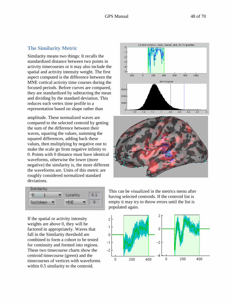
The Similarity Metric

Similarity means two things: It recalls the

standardized distance between two points in

activity timecourses or it may also include the

spatial and activity intensity weight. The first

aspect computed is the difference between the

MNE cortical activity time courses during the

focused periods. Before curves are compared,

they are standardized by subtracting the mean

and dividing by the standard deviation. This

reduces each vertex time profile to a

representation based on shape rather than

amplitude. These normalized waves are

compared to the selected centroid by getting

the sum of the difference between their

waves, squaring the values, summing the

squared differences, adding back these

values, then multiplying by negative one to

make the scale go from negative infinity to

0. Points with 0 distance must have identical

waveforms, otherwise the lower (more

negative) the similarity is, the more different

the waveforms are. Units of this metric are

roughly considered normalized standard

deviations.

This can be visualized in the metrics menu after

having selected centroids. If the centroid list is

empty it may try to throw errors until the list is

populated again.

If the spatial or activity intensity

weights are above 0, they will be

factored in appropriately. Waves that

fall in the Similarity threshold are

combined to form a cohort to be tested

for continuity and formed into regions.

These two timecourse charts show the

centroid timecourse (green) and the

timecourses of vertices with waveforms

within 0.5 similarity to the centroid.

GPS Manual 49 of 70

Procedure

1. Select the study, subject brain, and condition to make

regions for.

2. Load the metrics that will be used, at least including

MNE cortical activity.

3. Visualize the MNE cortical

activity.

4. Generate the Maximal Activity metric from one or more

datasets.

5. Generate a list of centroids as candidates to seed regions

of interest.

6. Select necessary

regions and examine

similarity.

7. Create (All) ROIs.

This will automatically

run.

8. Save labels in the saving menu. This step will also save a

screenshot of the current view and save a .mat file containing

data useful for downstream analysis.

GPS Manual 50 of 70

Chapter 7: Plot Drawing Interface

The plot drawing interface is a tool that loads the data produced by GPS Analysis and displays

graphs of Granger causality. Below, it is outlined each of the menus and the effects of each

option. This interface can be operated without MNE or Freesurfer as long as the subject’s MRI

files have already been processed and the final Granger results have been computed.

Figure 7.1 Granger Plot Drawing Open

GPS Manual 51 of 70

There are 3 main boxes on the screen. The buttons in “Features” select different menus to appear

down below. The box labeled “Dataset” in Figure 7.1 will display options for each feature. The

“Screenshot” box just contains fast shortcuts to take pictures of the circle & surface plots or the

timecourse plot.

Besides this menu figure, GPS: Plot Drawing has three more figures. The Circle or Surface

figure displays rendered graphical or neural displays of the data. The Timecourse figure shows

time courses indicated in the last feature button. At start, they are turned off by default but you

can change them in the menus.

The data figure will hold all of the data you select to load in the dataset menu. It will also contain

analysis made by the GUI. The reason these variables are stored in a separate figure window is

because, otherwise, the primary figure would be overburdened with memory-wanting variables

and it would act very slow. Do not close this window or you will lose your session’s data. It is

safe to minimize it.

Loading a Dataset

The Dataset menu provides functions for the user to load granger analysis for the conditions of a

study. The study list is populated by looking at the GPS parameters directory just like in GPS

Analysis. The condition list shows conditions for that study. Since conditions specify which

brain they have data analysis on, it can automatically figure out which freesurfer files to load.

Figure 7.2 Data figure

Figure 7.3 Dataset button and menu

GPS Manual 52 of 70

Clicking on the Load button next to Granger will open a dialog to select the file in which the

Granger data is held. If everything is built in GPS and the Analysis functions ran okay, then the

dialog should point to the correct file to open.

This folder is the condition.granger.dir/results folder. The original granger analysis is in the raw

directory and can also be opened by GPS: Plot Drawer. The null hypothesis data is in the

corresponding folder but takes too much time to load so that extra preparation step was built into

the GPS: Analysis routine.

The activation loading function will find the MNE cortical activation maps generated in the

MNE stage of the analysis. Right now, there is not support for comparing activation maps so the

comparison condition does not have that option.

The compare section has a dropdown list of all of the conditions compatible with the selected

condition for comparison. For instance, both conditions must be analyzed with the same cortical

surface.

Figure 7.4 Dataset file selection dialog

GPS Manual 53 of 70

Rendered “Surface” Plots

In order to see the neural activity on the brain or see nodes with granger causality flowing

between them, choose a surface in the surface menu. The cortical surface can display activation

as well as be drawn on by the visualization functions to illustrate causality. The circle display

just shows each region as a label around a circle and can display arrows or node sizes.

Options

Background: Allows you to choose the color for the background of the render.

Width: Attempt to make the plot a fixed width long.

Height:Attempt to make the plot a fixed width tall.

Portions:

o Left/Right: Include the left and/or the right hemisphere.

o Lateral/Medial: Display the surfaces from either perspective

Cortex Options

o Surface: Default “Inflated” this specifies which FS built cortical surface to view

o Gyri/Sulci: This option clarifies whether or not to partition the brain into gyri

and sulci by brightness.

o Shadows: Determines whether the rendering engine should spend time

making shadows. Turn this off if you want a more cartoony approach.

Cortical Atlas

o Freesurfer automatically generates a few atlases of the subject’s brain such as

coarse descriptions of primary anatomical areas. If you select an option other than

Figure 7.5 Surface button and menu

GPS Manual 54 of 70

none from the dropdown, it will draw an overlay of these regions on the cortical

images.

o Layer: Whether or not you want the atlas’s features to be shown on the

foreground (blended with cortical activation), background (blended with the

gyri/sulci overlay) or on top of it all.

o Border: If you want thicker borders to the regions, write a number between 1 and

10 in this box. For instance, your GPS Analysis processed ROIs will be available

as an atlas and you can visualize it in this rendering scheme.

o Show Labels: When this box is checked it will show the names of the labels.

o Just Primary: Turn this option on if you are selecting just one or a few of the

ROIs from the “Regions” menu and want to map only these primary ROIs on to

the cortical map.

Figure 7.6 A typical cortical surface display

Figure 7.7 Circle representation, showing granger causality directions as arrows

GPS Manual 55 of 70

Cortical Activity

This menu works only if you have loaded a cortical activity basis for the primary condition. If

you check the box “Show Activation,” the program will render cortical activation using a

standard heat map on the cortical surface. It will average it in the millisecond time window you

specify. Activity can be colored by percentage (P) thresholds or absolute value (V) thresholds.

At this monment the Show Colorbar box is disabled.

Figure 7.8 Cortical Activity button and menu

GPS Manual 56 of 70

Regions, selection and labels

Loading all of the granger connections at once can be daunting and incomprehensible. Thereby,

GPS allows you to select just a subset of your data to look at. The primary box shows all of the

ROIs of the condition you are analyzing. By selecting ROIs here, only granger connections

involving these ROIs will be displayed. The All, L, and R buttons select (or deselect) the whole

list, the left side, or the right side respectively.

The connections list contains a listing of all possible pairs involving the selected ROIs from the

primary listing. If you select the exclusive filter, it will only show possible pairs involving

combinations among selected ROIs. You can choose to ignore outbound or inbound connections

from your selected ROIs by unchecking that box. Checking the box Between hemis will only

display connections that stay in one hemisphere (eg. Left to left).

The labels box is a secondary way to label your regions, which options for font size and font

color.

Granger Process

The next two buttons open menus that help you manipulate the Granger connectivity data.

Figure 7.9 Regions button and menu

GPS Manual 57 of 70

Methodology

This option list helps you to properly format your data for visual analysis.

Options: Dropdown: The dropdown list lets you specify whether you are seeing your primary

condition, or your comparison condition.

GCI: Specify that time points are significant if the Granger Causality Index is above a

certain value. 0 is the baseline GCI, but numbers around 0.25 generally work in practice.

However, once you have run significance testing use P values.

P Value: Timepoints can be evaluated on how unusual they are from the null hypothesis

tests.

Time Window: This window cannot be edited, but it displays the information from the

time page.

Dropdown 2: This allows you to select whether you are counting the number of

significant timepoints, or whether you want to add suprathreshold values together.

Exclude connections with… This helps you to exclude weak connections from

visualization. The prob. same below option only works when there are p values for a

primary and comparison condition.

Figure 7.10 Method button and options

GPS Manual 58 of 70

Time

This feature allows you to specify which time window you are examining. In practice, you will

not modify this often. If you specify lower durations and intervals you can see more slices of the

granger interaction and you can use the slide to jump between time periods.

The timestamp option at the bottom is useful for understanding which time points are actually

going into your visualizations.

Granger Visualizations

There are three visualizations available to examine the data:

Figure 7.11 Time button and options

GPS Manual 59 of 70

Arrows

This feature set allows you to visualize Granger interactions as arrows. Arrows are useful in

showing the directionality of signals between ROIs

Options Show Arrows: Toggles the display on the cortical or circle surface

Terminal Wedge…: Allows you to choose among different arrow styles.

Green-Blue Gradient: Allows you to choose among different arrow colors. The

green/blue option is generally the most used option. Green represents signals leaving the

region, while blue represents signal arriving at the region.

Scaling: This option allows you to modify the size of the arrow in order to enhance

visualization; however it is advised that users keep the same scale across analysis.

Borders: Selecting this box will add borders to the arrows.

Label Weights:Check if you want values indicating magnitude displayed in each arrow.

Asterisks to show significance:If you are doing a comparative test, you can click this and

it will put asterisks in arrows based on if that relation is statistically important.

Figure 7.12 Arrows button and options

GPS Manual 60 of 70

Figure 7.13 shows what the arrows look like on a cortical surface. In this case, it is showing a

comparative analysis between the “all” and “correct” conditions. Green-Blue arrows show higher

“all” activity, Yellow-Magenta arrows show higher “correct” activity.

Nodes, “Bubbles”

Instead of arrows, values can be displayed as circles where the regions are located. They will be

colored the same way as the arrows but other options can change their behavior.

Options Outgoing: Toggle button for whether or not to show the sum of granger connection

indices (or the count of, depending on your method) starting at each node.

Figure 7.13 Cortical surface with arrows

Figure 7.14 Nodes button and options

GPS Manual 61 of 70

Incoming: Selecting this box will show the sum of granger connection indices ending at

each node.

Scaling: This section allows you to input a desirable scale for the circles in order to

enhance visualization; however it is advised that users keep the same scale across

analysis.

Circles overlaid… This menu presents with options of different ways that outgoing

and incoming summations can be visualized.

Don’t draw primary regions: Checking this box will only display circle on the ROIs that

are influenced by the selected ROIS, thus there will be no circles on top of selected ROIs

Borders: Checking this box will draw borders around the circles

Label weights: Add text indicating the values. Shown around label. It can be very

effective for giving summary statistics.

Asterisks…: Indicates comparative significance in circles/labels.

Time Courses

. There are a large number of options for this feature set. It will display the time courses for all of

the connections selected in the Regions menu. The solid line will show the GCI (or p-value, as

specified in the Method menu) and the dashed line will show the criteria (eg. a p-value of no

more than 0.05).

Options: Show Timecourses:Checking this box will open a timecourse figure.

Figure 7.15 Timecourses button and menu

GPS Manual 62 of 70

[ ] Plots: Allows you to input the number of plots to be generated, which can be

useful when viewing a lot of connections.

Fill: Fill the space the experimental values are above the criteria.

Reflections: Plot the reverse directions as well, on a flipped chart if you have also

selected tips only.

Tips Only: Selecting this option will only draw values within the criteria line, which

can make the chart much more tractable.

Signif. Spikes: Draw vertical lines where timepoints are significant

Plot P Values: Change the legend to p values as well as the nature of some of the

functions.

Log scale: Change the y axis to a logarithmic scale.

Flip Y Dir: Flip the direction of the Y axis

Right Y Axis: Show the Y axis on the other side of the screen

Legend: This menu allows user to choose where legend should be positioned

within the picture.

Y Bounds: The minimum and maximum for the plot

Background: This menu allows user to choose the background color for the graph.

Width: The approximate width of the plot

Height: The approximate height of the plot

Font: What font to render the names in. Some journals require specific fonts. Be

careful, this list is generated from your computer but not all fonts listed may render

corrected in Matlab.

GPS Manual 63 of 70

The following, are graphs for the sample data’s all and correct condition which the timecourse

settings to make those plots.

Figure 7.16 Timecourse options for Figure 7.17

Figure 7.17 Timecourse plots for L-STG to L-MTG1 (Red) and L_MTG2 (Cyan) for WPM

“all” (Left) and “correct” (Right) conditions.

GPS Manual 64 of 70

Appendix 1: Remote Connecting

This section applies to Martinos Center users only.

In order to access the graphical processing stream from a personal computer or a machine not

directly connected to the Martinos network, one needs to build a network bridge to the center.

There are a few different ways to remotely connect; this section will highlight the most used

ones. This presumes that you have access to a Martinos network computer Linux computer. This

manual should provide you all of the necessary information but in case you run into any

problems or want more options you may consult the Martinos documentation for remote

connections.

http://www.nmr.mgh.harvard.edu/martinos/userInfo/computer/remoteAccess.php

Secure Shell (SSH)

The simplest way to connect to a Martinos network computer is using the Secure Shell protocol,

shortened as SSH. This will open a session identical to operating a terminal (shell) client on the

Linux machine itself.

Windows

Users of the Windows operating system will

need to use PuTTY or a similar SSH client to

connect to a computer on the Martinos network.

This may be downloaded here:

http://www.chiark.greenend.org.uk/~sgtatham/p

utty/download.html

The first step in connecting is to establish a

session with the Martinos network gateway, that

is the servers door, entry, or gate. Do not do

analysis on these computers, but use this to get

into the network. Open up PuTTY. Specify the

hostname as <server>.nmr.mgh.harvard.edu

and the port as number 22.

Enter your username and password. Once you are connected, directly connect to the computer by

using the ssh command within terminal. The command is ssh <servername>. You will be

prompted to enter your password again.

GPS Manual 65 of 70

Macintosh and Linux

It is much easier to connect on a Macintosh or Linux computer. Since they are built on a Unix

kernel and have similar design elements, you can connect to the Martinos network with the

native Terminal program. To connect to an internal server connect to a gateway first. The

command to connect is

ssh <username>@<server>.nmr.mgh.harvard.edu

Virtual Network Computing (VNC)

This approach will enable you to open a desktop session on the remote computer that will appear

as a window. In order to start a VNC session you may need to set it up your VNC parameters on

your user account in the Martinos network. To start a session, open a terminal to the computer

that you want to host the session

or SSH into that computer. Start

the VNC server by typing the

command vncserver :<num>,

where the number is a value

between 1 and 99 that no other

user will use. This server will

create a session in the remote

connecting port of that number.

In order to terminate an

existing vncserver connection,

terminate the process using

the same command as before

but adding the kill option: vncserver –kill :<num>

Windows

Back at the computer that is opening the remote connection, you will need to open an SSH

session that bridges the VNC connection and then open a VNC viewer. Load the previous

session information in which you connect to a Martinos gateway. In the configuration, go to the

options for Connection/SSH/Tunnels and add a new forwarded port whose source port is 59XX,

in which the number you choose above fills the tens digit. The destination is the desktop you

GPS Manual 66 of 70

started the vncserver session at then the appropriate 59XX number again. Add this to the list of

forwarded ports, save the session and go.

Now, your computer will need a program that

can open VNC sessions. One such program is

called Tight VNC. Connect to the remote host

<desktop>:<num> and enter your VNC

password. Note that when you first use VNC

you will set up your VNC password and this

does not need to change –unlock your Martinos

account password. Click OK and the program

will open a remote desktop session.

http://www.tightvnc.com/

Macintosh

Chicken of the VNC offers a much easier client to connect to VNC sessions. The SSH

connection is provided by the program. Just enter the destination computer, connection port

number, VNC password, and toggle the

SSH options and enter the SSH host as <username>@

<server>.nmr.mgh.harvard.edu .

When the session starts it will prompt for

your Martinos center password.

http://sourceforge.net/projects/chicken/

GPS Manual 67 of 70

File Transfer Protocol (FTP) – Windows

In order to transfer files between the Martinos

network and you computers you will want to use

a file transferring client. On Windows

computers, WinSCP offers a great client for

crossing servers. You will want to connect to

one of the gateway servers.

http://sourceforge.net/projects/winscp/

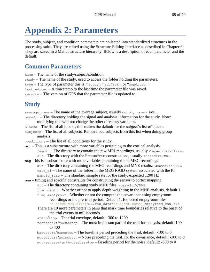
GPS Manual 68 of 70

Appendix 2: Parameters

The study, subject, and condition parameters are collected into standardized structures in the

processing suite. They are edited using the Structure Editing Interface as described in Chapter 6.

They are saved in a Matlab structure hierarchy. Below is a description of each parameter and the

default.

Common Parameters

name – The name of the study/subject/condition.

study – The name of the study, used to access the folder holding the parameters.

type – The type of parameter this is. “study”, “subject”, or “condition”

last_edited – A timestamp to the last time the parameter file was saved.

version – The version of GPS that the parameter file is updated to.

Study

average_name – The name of the average subject, usually <study name>_ave.

basedir – The directory holding the signal and analysis information for the study. Note:

modifying this will not change the other directory variables.

blocks – The list of all blocks, this makes the default for the subject’s list of blocks.

subjects – The list of all subjects. Remove bad subjects from this list when doing group

analysis.

conditions – The list of all conditions for the study.

mri – This is a substructure with more variables pertaining to the cortical analysis

rawdir – The directory to contain the raw MRI recordings, usually <basedir>/MRIraw.

dir – The directory with the Freesurfer reconstructions, usually <basedir>/MRI.

meg – his is a substructure with more variables pertaining to the MEG recordings

dir – The directory containing the MEG recordings and MNE results, <basedir>/MEG.

raid_pi – The name of the folder in the MEG RAID system associated with the PI.

sample_rate – The standard sample rate for the study, expected 1200 Hz

mne – timing and specific constraints for constructing the sensor to cortex mapping

dir – The directory containing study MNE files. <basedir>/MNE.

flag_depth – Whether or not to apply depth weighting in the MNE analysis, default 1.

flag_emptyroom – Whether or not the compute the covariance using emptyroom

recordings or the pre-trial period. Default 1. Expected emptyroom files: <subject.meg.dir>/MEG/raw_data/<subject.name>_emptyroom_raw.fif

There are 10 more parameters in pairs that mark time boundaries relative to the onset of

the trial events in milliseconds.

start/stop – The trial envelope, default: -300 to 1200

focusstart/focusstop – The most important part of the trial for analysis, default: 100

to 400

basestart/basestop – The baseline period preceding the trial, default: -100 to 0

noisestart/noisestop – Noise preceding the trial, for the covariance, default: -300 to 0

noiasebasestart/noisebasetop – Baseline period for the noise, default: -300 to 0

GPS Manual 69 of 70

plv – this is a substructure with variables pertaining to phase locking analysis

dir – The directory containing the PLV trials and results, default: <basedir>/PLV.

frequencies – List of the frequencies PLV is being done in.

flag – A temporary flag to indicated whether or not PLV analysis is being done, defunct.

granger – this is a substructure with variables pertaining to Granger analysis

dir – The directory containing the Granger data, default: <basedir>/Granger.

model_order – The number of time lags for the Kalman filter, default: 5

W_gain – An adjustable variable for the Kalman filter, default: 0.5

N_comp – The number of iterations for the null hypothesis training, default: 0.5

plv_freq – The frequency used if incorporating PLV in the granger ROIs, default: 0.5

srcs – String pattern to match Granger-causality causing regions to

snks – String pattern to match Granger-causality receiving regions to.

singlesubject – An adjustable flag for the Granger analysis, default: 0 (False)

Subject

blocks – The list of successful blocks the subject has. Default is the list of all from the study.

mri – This is a substructure with variables pertaining to the cortical analysis.

rawdir – The directory to contain the raw MRI recordings, default

<study.mri.rawdir>/<subject.name>.

sourcedir – The folder that the MRI recordings originate from

first_mpragefile – The first (or only) file that the T1 MPRAGE MRI scan is located.

dir – The directory with the Freesurfer reconstructions, default

<study.mri.dir>/<subject.name>.

corfile – The file with the MEG-MRI coregistration

ico – The density of the decimated vertices. Default: 7

meg – his is a substructure with more variables pertaining to the MEG recordings

raid – The MEG RAID server the subject’s data is hosted on.

dir – The directory containing the MEG recordings and MNE results,

<study.meg.dir>/<subject.name>.

sourcedir – The directory the MEG recordings were copied from.

bad_eeg – list of the numbers designations of the bad EEG channels.

bad_meg – list of the numbers designations of the bad MEG channels.

sample_rate – The sample rate of the MEG recordings for the subject.

projfile – The .fif file containing the EOG projections, declared in the analysis stage.

behav – A structure containing custom behavioral data, made while processing events.

mne – timing and specific constraints for constructing the sensor to cortex mapping

dir – The directory containing study MNE files. Default: <study.mne.dir>/<subject.name>

avefile – The file with primary condition sensor averages.

covfile – The covariance file used in the MNE inverse model.

fwdfile – The file containing the forward model, mapping cortex to sensor activity.

invfile – The file containing the inverse model, mapping sensor to cortex activity.

plv – this is a substructure with variables pertaining to phase locking analysis

sample_rate – Defunct.

sample_times – The times for each sample relative to the trial onset.

GPS Manual 70 of 70

Condition

level – Numeric assignment to which level the condition is on. 1 means primary – should be

used in constructing the inverse solution, 2 means secondary – distinct set of trials to

generate source timecourses, 3 is a placeholder and may be implemented to mean tertiary

– a time subset of a secondary trial.

event – This is a substructure with variables pertaining to determining the evoked period

desc – A description of the event if not the condition name itself. Saved in –ave.fif file

during the MNE/average_waves function.

code – The numeric codes corresponding the grouped event numbers to this condition.

There are 6 more parameters in pairs that mark time boundaries relative to the onset of

the trial events in milliseconds. They are based on the study’s times.

start/stop – The trial envelope, default: -300 to 1200

focusstart/focusstop – The most important part of the trial for analysis, default: 100

to 400

basestart/basestop – The baseline period preceding the trial, default: -100 to 0

cortex – This is a substructure with variables pertaining to cortical estimates

brain – The cortical service the condition is meant for, usually average but it may be

subject relevant.

plvrefdir – The location to where the average PLV reference label(s) are located.

Default: <study.plv.dir>/rois/<condition.name>.

roidir – Old way to organize ROIs, this is a pointer to the ROI directory.

roiset – This new way expects the ROI labels (and data .mat file) to be in the

<study.granger.dir>/rois/<condition.cortex.roiset>. This change was

made when it was apparently that more conditions may be pointed to the same set

of regions. The default is just the condition name.

granger – This is a substructure with variables relevant to Granger analysis.

subsets – Divisions in time for the Granger analysis if relevant. Otherwise empty.

The next three parameters are pointers to files for the Granger processing. Right now

gps_filename.m or gpsa_granger_filename.m will automatically determine

the Granger filenames so these parameters are not used.

input – The file with the collection of ROI timecourses for input to Granger analysis.

output – The file with the results of the Granger analysis.

signif – The file with Granger null hypotheses for significance testing.