granger causality and national procurement … spending time series data that can improve...

DraftCopy

Défense

nationale

National

Defence

Defence R&D CanadaCentre for Operational Research and Analysis

Materiel Group Operational ResearchAssistant Deputy Minister (Materiel)

DRDC CORA TM 2011-154September 2011

Granger Causality and NationalProcurement SpendingApplications to the CC130 Hercules Fleet Performance

David W. MayburyMateriel Group Operational Research

DraftCopy

DraftCopy

Granger Causality and National ProcurementSpendingApplications to the CC130 Hercules Fleet Performance

David W. MayburyMateriel Group Operational Research

Defence R&D Canada – CORATechnical MemorandumDRDC CORA TM 2011-154September 2011

DraftCopy

Principal Author

Original signed by David W. Maybury

David W. Maybury

Approved by

Original signed by R.M.H. Burton

R.M.H. Burton

Section Head (Joint Systems Analysis)

Approved for release by

Original signed by P. Comeau

P. Comeau

Chief Scientist

c© Her Majesty the Queen in Right of Canada as represented by the Minister of National

Defence, 2011

c© Sa Majesté la Reine (en droit du Canada), telle que représentée par le ministre de la

Défense nationale, 2011

DraftCopy

Abstract

Using Granger causality tests, we look for relationships in performance and National Pro-

curement spending time series data that can improve forecasting capabilities with the CC130

fleet. We find that no meaningful relationships exist between spending and performance in-

dicators within the spending envelope studied. Our results concord with earlier work based

on random matrix theory and minimal spanning trees, which suggest the fleet is robust to

spending shocks. We conclude that NP spending changes do not correlate with subsequent

CC130 Hercules aircraft performance changes and vice versa. Granger causality tests rep-

resent a powerful tool which can be used with future fleet studies.

Résumé

Nous avons recours à des tests de causalité à la Granger pour établir des liens entre les

données de séries chronologiques sur le rendement et les dépenses d’approvisionnement

national qui permettraient d’améliorer les capacités de prévision pour la flotte des CC130.

Nous constatons qu’il n’existe aucun lien significatif entre les dépenses et les indicateurs

de rendement performance au sein de l’enveloppe de dépenses étudiée. Nos résultats sont

conformes à ceux de recherches antérieures fondées sur la théorie des matrices aléatoires

et sur les arbres de poids minimum, et selon lesquelles la flotte résiste aux réductions des

dépenses. Nous pouvons conclure que les fluctuations des dépenses d’approvisionnement

national et les fluctuations ultérieures du rendement des avions CC130 Hercules ne sont

pas corrélées, et inversement. Les tests de causalité à la Granger constituent un puissant

outil qui pourra servir dans les futures études de flotte.

DRDC CORA TM 2011-154 i

DraftCopy

This page intentionally left blank.

ii DRDC CORA TM 2011-154

DraftCopy

Executive summary

Granger Causality and National Procurement SpendingDavid W. Maybury; DRDC CORA TM 2011-154; Defence R&D Canada – CORA;September 2011.

ADM(Mat) has sought a deeper understanding of the relationship between National Pro-

curement (NP) spending and fleet performance across the Canadian Forces for the last eight

years. Senior decision-makers have hoped that insight into spending effects on fleet oper-

ations would eventually lead to better sparing methodologies, more efficient maintenance

activities and schedules, along with a deeper understanding of end-of-life issues. Using the

CC130 NP spending and performance data, we re-examine the results in [2] by applying

econometric times series methods.

We search for relationships between time series by using Granger causality tests, which

tells us if the mean squared forecasting error of one time series can be reduced through

knowledge of another time series. This study provides a complement to [2] and we show

that NP spending does not improve the predictability of any time series. We find that no

meaningful relationships exist between spending and performance indicators within the

spending envelope studied.

We should stress that not discovering Granger causality in spending and fleet performance

data does not imply inefficiency. In fact, an efficiently maintained fleet should not show

a strong correlation between routine spending and performance changes. On the other

hand, we caution that these results do not imply that the underlying supply chain is optimal

– the robustness to spending shocks may simply arise from non-optimally high inventory

levels. We cannot address supply chain issues or optimal sparing through Granger causality

tests. From the analysis in this study, we can only conclude that NP spending changes

do not correlate with subsequent performance changes and vice versa. Further analysis

is warranted on the supply chain to understand the reasons behind the lack of Granger

causality.

DRDC CORA TM 2011-154 iii

DraftCopy

Sommaire

Granger Causality and National Procurement SpendingDavid W. Maybury ; DRDC CORA TM 2011-154 ; R & D pour la défense Canada –CARO ; septembre 2011.

Au cours des huit dernières années, le SMA(Mat) a voulu mieux comprendre les liens entre

les dépenses d’approvisionnement national et le rendement de la flotte dans l’ensemble

des Forces canadiennes. Les décideurs principaux espéraient que de mieux comprendre

les effets des dépenses sur la flotte permettrait de mieux définir les quantités optimales de

pièces de rechange à garder en stock, d’améliorer l’efficacité des activités et des calendriers

d’entretien et de mieux comprendre les problèmes associés à la fin de vie utile. À l’aide des

données sur le rendement de la flotte de CC130 et sur les dépenses d’approvisionnement

national connexes, nous réexaminons les résultats obtenus [2] en appliquant les méthodes

économétriques de séries chronologiques.

Nous vérifions s’il existe des liens entre les séries chronologiques au moyen des tests de

causalité à la Granger, qui permettront de déterminer si l’erreur quadratique moyenne de

prévision d’une série chronologique peut être réduite par l’introduction d’une autre série

chronologique. La présente étude se veut un complément de [2], et nous y démontrons

que les dépenses d’approvisionnement national n’améliorent pas la prévisibilité des séries

chronologiques. Nous constatons qu’il n’existe aucun lien significatif entre les dépenses et

les indicateurs de rendement performance au sein de l’enveloppe de dépenses étudiée.

Nous devons souligner que l’absence d’un lien de causalité à la Granger entre les dépenses

et le rendement de la flotte n’est pas synonyme d’inefficacité. En fait, dans le cas d’une

flotte entretenue de façon efficiente, une forte corrélation entre les dépenses courantes et

les fluctuations du rendement ne devrait pas être observée. Une mise en garde s’impose

toutefois : les résultats ne devraient pas porter à croire que la chaîne d’approvisionnement

sous jacente est optimale - la résistance aux chocs de dépenses peut simplement s’expliquer

par des stocks trop grands. Les tests de causalité à la Granger ne permettent pas de traiter les

questions relatives à la chaîne d’approvisionnement ou aux quantités optimales de pièces de

rechange à garder en stock. La seule conclusion pouvant être tirée de la présente analyse est

que les dépenses d’approvisionnement national et les fluctuations ultérieures du rendement

ne sont pas corrélées, et inversement. D’autres études sur la chaîne d’approvisionnement

devront chercher à comprendre l’absence d’un lien de causalité à la Granger.

iv DRDC CORA TM 2011-154

DraftCopy

Table of contents

Abstract . . . . . . . . . . . . . . . . . . . . . . . . . . . . . . . . . . . . . . . . . i

Résumé . . . . . . . . . . . . . . . . . . . . . . . . . . . . . . . . . . . . . . . . . i

Executive summary . . . . . . . . . . . . . . . . . . . . . . . . . . . . . . . . . . . iii

Sommaire . . . . . . . . . . . . . . . . . . . . . . . . . . . . . . . . . . . . . . . . iv

Table of contents . . . . . . . . . . . . . . . . . . . . . . . . . . . . . . . . . . . . v

Acknowledgements . . . . . . . . . . . . . . . . . . . . . . . . . . . . . . . . . . . vi

1 Introduction . . . . . . . . . . . . . . . . . . . . . . . . . . . . . . . . . . . . . 1

1.1 Background . . . . . . . . . . . . . . . . . . . . . . . . . . . . . . . . . 1

1.2 Scope . . . . . . . . . . . . . . . . . . . . . . . . . . . . . . . . . . . . . 2

2 Results . . . . . . . . . . . . . . . . . . . . . . . . . . . . . . . . . . . . . . . . 3

2.1 Data selection . . . . . . . . . . . . . . . . . . . . . . . . . . . . . . . . 4

2.2 Analysis . . . . . . . . . . . . . . . . . . . . . . . . . . . . . . . . . . . 5

3 Conclusions . . . . . . . . . . . . . . . . . . . . . . . . . . . . . . . . . . . . . 10

References . . . . . . . . . . . . . . . . . . . . . . . . . . . . . . . . . . . . . . . . 12

Annex A: Time series and Granger causality . . . . . . . . . . . . . . . . . . . . . 13

Annex B: Fleet indicator definitions . . . . . . . . . . . . . . . . . . . . . . . . . . 17

List of Acronyms . . . . . . . . . . . . . . . . . . . . . . . . . . . . . . . . . . . . 22

DRDC CORA TM 2011-154 v

DraftCopy

Acknowledgements

I would like to thank Dr. Ben Solomon for useful discussions and his encouragement during

this project.

vi DRDC CORA TM 2011-154

DraftCopy

1 Introduction

It would be nice to use a non-parametric approach – just use histograms to characterize the jointdensity . . . Unfortunately, we will not have enough data to follow this approach in macroeconomicsfor 2000 years or so.

— John H. Cochrane

1.1 BackgroundADM(Mat) has sought a deeper understanding of the relationship between National Pro-

curement (NP) spending and fleet performance across the Canadian Forces for the last eight

years. Senior decision-makers have hoped that insight into spending effects on fleet oper-

ations would eventually lead to better sparing methodologies, more efficient maintenance

activities and schedules, along with a deeper understanding of end-of-life issues. In a pe-

riod of budget restraints, ADM(Mat) requires an analysis of the effect that changes in NP

spending have on DND fleets. In response to ADM(Mat)’s concerns, the Directorate of

Materiel Group Operational Research (DMGOR) has applied numerous technical methods

to fleet data over the last five years, including neural networks trained on performance and

costing data, generalized filter methods, and asymptotic methods based on equilibrium re-

laxation of coupled differential equations [1]. Despite the incredible efforts, each method

has failed to identify a compelling link between high level performance indicators and NP

spending.

Last year, the DMGOR undertook a study to elucidate spending linkages with performance

data by examining the correlation structure of NP spending and performance time series

data with the CC130 fleet. In [2], the DMGOR found that the correlation matrix for CC130

fleet performance with NP spending data contained a significant amount of noise dressing,

which impedes the development of a general filter method. By constructing a minimal

spanning tree on an ultrametric space in which the performance indicators and NP spending

formed nodes, the DMGOR found that NP spending did not form a hub or cluster with the

performance data. As a result, it was concluded in [2] that NP spending changes do not

provide a meaningful input to predicting future performance changes.

While the problem seems well posed and the result of [2] counterintuitive, any potential

analysis that attempts to isolate the effect of spending levels on fleet performance faces ex-

treme hurdles. Since spending connects to a myriad of exogenous economic factors, such

as inflation, price fluctuations in materiel, and worldwide supply chain pressures, a simple

one-to-one map cannot exist between spending and any performance measure1. For exam-

ple, in any one period, spending may rise as the result of an increase in the cost of lubricants

1We suffer from simultaneous equation bias under which the error term in a regression analysis is cor-

related with the explanatory variable. Simultaneous equation bias plagues the social sciences as we cannot

usually perform a controlled experiment.

DRDC CORA TM 2011-154 1

DraftCopy

while performance may decline due to the discovery of an unexpected aging effect. The

problem of connecting NP spending to fleet performance must rely on a statistical analysis

of changes in both fleet indicators and costs as primary inputs.

This paper re-examines the results in [2]. Instead of focusing on the correlation matrix’s

structure, we search for relationships in vector autoregressive models of the performance

and NP spending time series data. In particular, we apply statistical tests that identify if

knowledge of the NP time series improves the prediction of the high level performance

indicators. This study provides a complement to [2] and we show that NP spending does

not improve the predictability of any CC130 performance time series.

1.2 ScopeADM(Mat) requires a study to identify possible exploitable information between NP spend-

ing and fleet performance. In particular, a former COS(Mat) [3] tasked the DMGOR to

search for a methodology that would allow a more logical articulation of the linkage be-

tween the resources allocated to National Procurement. In discussions with the former

DCOS(Mat), the CC130 Hercules fleet was identified as a priority for the previous study

[2]. We extend the analysis in [2] using time series techniques. Our modelling methods

aim to:

• use the theory of time series to identify if the mean squared error (MSE) in the predic-

tion of changes in the performance time series data are reduced through knowledge

of changes in total NP spending; and

• identify how the results of [2] concord with this study

We obtained all performance data on the CC130 from the AEPM PERFORMA database

[4] and NP data from Financial and Managerial Accounting System (FMAS) [5].

We organize the paper in two parts. Following the introduction we informally discuss

Granger causality and display key results. Section 3, contains the conclusions and discusses

future avenues for research. We reserve the Annex A and annex B for technical discussions

on time series statistical test, and for definitions of the performance indicators respectively.

2 DRDC CORA TM 2011-154

DraftCopy

2 Results

In [2], it was determined through random matrix theory that the univarite innovations in

changes in NP spending did not correlate with subsequent univarite innovations in the per-

formance change data. The analysis told us that the majority of observed cross-correlations

were spurious and could mostly be explained through noise dressing. Furthermore, NP

spending did not form a central hub in the minimal spanning tree analysis [2]. These ob-

servations suggest that knowledge of changes in NP spending does not improve forecasting

changes in the performance time series data.

We seek a further understanding of relationships in the performance and NP spending data

using the theory of time series analysis. In particular, we use Granger causality tests [6]

to search for information in one time series that can improve the forecast of another time

series. We will see that Granger causality tests provide a excellent complement to the work

in [2].

The concept of Granger causality rests on the ability to use the past knowledge in one time

series to help improve the forecast of another time series. It is true that if one time series

actually causes another time series then knowledge of the driving time series will improve

the forecasts, but Granger causality does not give us actual causal information. In fact,

causality is not something that we can test for statistically, but must be known a priori. An

example will help illustrate Granger causality.

Imagine that we have built a crude home-made weather station that we use to predict the

weather. We make observations and compare our recordings with our predictions. Our only

source of information to make forecasts comes from our weather station, which includes all

past observations. Now, suppose that we decide to include Environment Canada’s weather

observations in our information set when we make a forecast. Given that Environment

Canada has state-of-the-art meteorological equipment, the inclusion of their observations in

our forecast will almost certainly improve our prediction of the weather. From a time series

perspective, Environment Canada’s observations Granger cause the weather time series

generated by our home-made weather station – we can improve our forecast through the

knowledge of Environment Canada’s data. The improved weather forecast does not mean

that Environment Canada actually causes the weather (after all, shooting the weatherman

will not stop the weather), but positive Granger causality effects between the time series

imply that we have found a mechanism for reducing the MSE in our forecasts. Clearly, we

should use this extra information if we are serious about predicting the weather. Granger

causality tests help us establish relevant information and relationships within multiple time

series data.

Armed with Granger causality tests, we can now rephrase the problem and search for rela-

tionships that extend the findings of the random matrix theory approach and minimal span-

ning tree technique. Using the theory of time series will provide us with a more refined


DraftCopy

analysis and allow us to dive deeper into the data as we search for meaningful relationships.

Granger causality methods can be applied generally at CORA across problems which have

multiple time series data.

2.1 Data selectionThis study uses two data sources for the CC130 fleet: the PERFORMA database for fleet

performance indicators, and FMAS for NP spending levels. In total, we select the same 13

high level performance indicators in [2], and we search for connections in the time series

data. Furthermore, we break down the NP spending into spares and R&O to help identify

relationships within spending subsets. For this study, we use cost centres:

• 8485QA: CC130 Spares;

• 8485QB: T56 Engine Spares;

• 8485QH: CC130 Airframe Repair and Overhaul;

• 8485QJ: CC130 Miscellaneous Engine;

• 8485QL: CC130 T56 Engine Repair and Overhaul;

• 8485TM: Repair and Overhaul Flight Navigation Communication Equipment and;

• 8485UQ: CC130 Ties.

In the total NP part of the study, we used the data from all cost centres while in the

spares/R&O breakdown part of the study we use 8485QA, 8485QB, and 8485QH, 8485QJ,

8485QL respectively.

We use the PERFORMA database to extract 10 years of monthly data (December of 1998

to November 2008, representing the same data set as [2]) for the performance indicators,

thereby giving us 120 measurements. In the data selection process, we need to ensure that

time series data captures the fleet’s performance at a high level with an expectation that NP

spending has an effect on the indicators themselves. The performance indicators we use

are:

1. All failures

2. Ao – Overall operational availability

3. Corrective maintenance person-hours rate

4. First level Ao

5. Flying hours


DraftCopy

6. Mean flying time between on aircraft corrective forms

7. Mean flying time between on aircraft preventive forms

8. Mean flying time between downing event

9. Off aircraft maintenance person-hour rate

10. On aircraft maintenance person-hour rate

11. On aircraft robs maintenance person-hour rate

12. Operation mission abort rate

13. Preventive maintenance person-hour rate

A full description of each performance indicator can be found in Annex B. The data we

select from the PERFORMA database concords with the type of data examined in past

attempts that address the NP allocation problem. Applying time series methods to the data

expands not only on the work in [1], but also on previous (unpublished) work that focused

on Ao as the main object to connect with NP spending [1].

We obtained the financial data from FMAS broken down by spares and R&O. The data

covers the same time frame (in monthly form) as the performance indicator data. The

financial data are placed inside a 13 month year to account for spending invoiced at the end

of one fiscal year but expensed in the following fiscal year. We correct for the 13 month

year by placing the data from the 13th month into the first month of the new fiscal year. We

understand that from an accounting perspective the 13th month represents a separate entity

to capture actual previous fiscal year spending relationships, but for our study, we need

to treat spending as a continuous process. Moving the 13th month spending into the first

fiscal month of the following year has the effect of removing the artificial discontinuous

seasonal jump that we see in the spending data at fiscal year changes. Since we desire

a relationship between incremental changes in the data, we must ensure that we make

appropriate comparisons with continuous time. We treat spending on spares, spending on

R&O, and total NP spending separately in the analysis.

2.2 AnalysisWe break the analysis down into three parts: performance indicators with total NP spend-

ing, performance indicators with spares spending, and performance indicators with R&O

spending. Before we apply time series modelling, we need to put the data in a standard

form through the transformation,

yi(t) = log

(xi+1

xi

), (1)


DraftCopy

where xi denotes the individual time series values. As we are not interested in absolute

levels2, eq.(1) ensures that we compare changes in NP spending to changes in performance

time series. In the small change approximation, eq.(1) expresses the percent change in the

time series level. The effect of changes represent the relationships that we wish to exam-

ine. To perform our analysis, we use MATLAB R©’s Econometrics Toolbox, and Statistics

Toolbox which contain all the routines needed for detailed time series analysis.

We test the transformed data for stationarity by using the augmented Dickey-Fuller test

(see [7] for details) with lags from 0 to 14 to assess the null hypothesis of a unit root with

and without drift. We find that we can reject the null hypothesis at the 95% confidence

level for all of the time series studied. Thus, we accept that each time series is stationary.

Next, we create 14 bivariate time series, pairing NP spending with each performance in-

dicator. Using the Akaike information criterion, we determine the best fit bivariate model

for each of the 14 cases. In each case, we test the residuals of the best fit model for het-

eroskedasticity using Engle’s ARCH test to detect model misspecification. We find that we

cannot reject the null hypothesis of no ARCH effects at the 95% confidence level in each

case of the 14 cases and thus we accept each best fit VAR model.

Using the F-test, we test each VAR model for Granger causality under the null hypothesis

that NP spending does not Granger cause any performance time series. Since we perform

14 F-tests in each spending-performance time series anlaysis, we use the 99% critical value

of the F-test to prevent rejecting the null hypothesis through type I errors.

In Table 1, we show the F-test results for Granger causality on all bivariate models of per-

formance with NP, spares and R&O spending. For total NP spending, we cannot reject the

null hypothesis of no Granger causality at the 99% confidence level (or at the 95% confi-

dence level). Thus, changes in NP spending do not Granger cause any of the changes in

performance indicators, which means that we cannot improve the linear forecast of per-

formance based on knowledge of the changes in the NP spending time series. We also

see that changes in spending on spares do not Granger cause changes in performance. For

each case, we test the robustness of the results by changing the lags in the best fit models

by two units in each direction around the Akaike information criterion. In all cases, the

acceptance of the null for NP and spares spending is maintained. However, at the 99%

confidence level, we see that changes in R&O spending allow us to reject the null hypoth-

esis of no Granger causality for changes in Flying Hours (TS5) and changes in Operation

Mission Abort Rate (TS12). While the result suggests that we can use R&O spending to

help improve the forecast of Flying Hours and Operation Mission Abort Rate, the results

are not robust under a sensitivity analysis around the minimum of the Akaike information

criterion. If we change the best fit model by two lags in either direction, the rejection of

the null hypothesis disappears. Since we have no underlying model linking any of the per-

formance indicators to R&O spending, the lack of robustness in the result tells us that we

2The client is concerned with the effect of changes in performance from changes in spending.


DraftCopy

Tab

le1:Granger

causality

F-test(S

pen

dingGranger

causingperform

ance

)

Fvalue

TS1

TS2

TS3

TS4

TS5

TS6

TS7

TS8

TS9

TS10

TS11

TS12

TS13

Tota

lNP

Spen

ding

F 0.99

2.4093

3.2002

2.3638

3.2002

2.7064

2.7064

2.8292

3.2002

3.2002

2.7064

3.2002

2.9877

2.7064

F-value

0.8181

0.6186

1.4290

0.5348

1.7829

1.3435

1.3641

1.6711

0.3447

0.9124

0.4707

1.1610

0.443

Spar

esSp

endi

ngF 0

.99

2.3258

3.2002

2.3258

3.2002

2.3258

2.7064

2.7064

3.2002

2.3258

2.7064

2.3258

2.3258

2.3638

F-value

0.9060

0.9330

0.5890

0.9539

0.6363

1.6719

1.0322

0.9780

0.7059

1.6759

1.1728

0.8816

0.8472

R&

OSp

endi

ngF 0

.99

2.3258

2.9877

2.3638

3.2002

2.70

642.7064

2.8292

3.2002

3.2002

2.7064

3.2002

2.52

912.4637

F-value

0.9849

1.0728

1.9753

0.8868

2.71

651.9515

1.5998

2.9922

1.8439

1.3955

0.4714

2.95

251.8261


DraftCopy

should cautiously reject the conclusion that R&O spending Granger causes Flying Hours

or the Operation Mission Abort Rate. These two time series should be flagged for future

analysis.

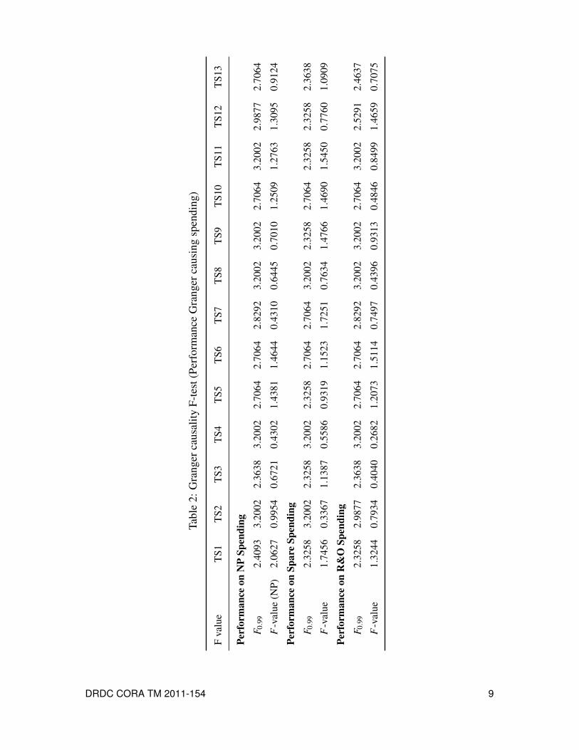
Finally, we turn the problem around to see if changes in one of the performance indicators

Granger cause spending changes. In table 2 we see that we cannot reject the null hypothesis

of no Granger causality. Again, the results are robust under changing the lags by two unit

in each direction.


DraftCopy

Tab

le2:Granger

causality

F-test(P

erform

ance

Granger

causingsp

ending)

Fvalue

TS1

TS2

TS3

TS4

TS5

TS6

TS7

TS8

TS9

TS10

TS11

TS12

TS13

Perf

orm

ance

onN

PSp

endi

ngF 0

.99

2.4093

3.2002

2.3638

3.2002

2.7064

2.7064

2.8292

3.2002

3.2002

2.7064

3.2002

2.9877

2.7064

F-value(N

P)

2.0627

0.9954

0.6721

0.4302

1.4381

1.4644

0.4310

0.6445

0.7010

1.2509

1.2763

1.3095

0.9124

Perf

orm

ance

onSp

are

Spen

ding

F 0.99

2.3258

3.2002

2.3258

3.2002

2.3258

2.7064

2.7064

3.2002

2.3258

2.7064

2.3258

2.3258

2.3638

F-value

1.7456

0.3367

1.1387

0.5586

0.9319

1.1523

1.7251

0.7634

1.4766

1.4690

1.5450

0.7760

1.0909

Perf

orm

ance

onR

&O

Spen

ding

F 0.99

2.3258

2.9877

2.3638

3.2002

2.7064

2.7064

2.8292

3.2002

3.2002

2.7064

3.2002

2.5291

2.4637

F-value

1.3244

0.7934

0.4040

0.2682

1.2073

1.5114

0.7497

0.4396

0.9313

0.4846

0.8499

1.4659

0.7075


DraftCopy

3 Conclusions

Searching for a connection between NP spending and fleet performance indicators repre-

sents a difficult problem. Past attempts, based largely on filter methods, have met defence

scientists with frustration. In 2010, the DMGOR re-analyzed the problem from a random

matrix theory and a minimal spanning tree approach [2] and found that NP spending was

not strongly linked to any performance indicator. In particular, [2] discovered that the uni-

varite spending innovations were not correlated with subsequent performance time series

innovations in any meaningful way.

The application of Granger causality test provides a new method for looking at spending

and performance data. Granger causality tells us which time series contain information

that allow us to reduce the MSE forecasting error in another time series. The application

of this technique to spending and CC130 fleet performance data from December 1998 to

November 2008 confirms the results in [2] and provides the CF with a new tool to help

search for relationships in time series data. In our analysis, we found that (R&O) spending

potentially Granger causes Flying Hours and the Operation Mission Abort Rate, yet the

effect disappears under slight model respecifications. This result suggests that we focus

on these time series in future analysis. Interestingly, the Operation Mission Abort Rate

appears close to (R&O) spending in the dendrogram in [2] (although not part of a central

hub).

We must stress that Granger causality does not tell us anything about actual causality or the

direction of any causal relationships. For example, it has been shown (see [7]) that stock

prices Granger cause dividends when in reality it is the market’s assessment of dividend

policies that set stock prices. This observation shows that Granger causality can mix up the

real underlying causal direction. Granger causality tests can help us understand forward

looking effects in the data. In the stock price and dividend example, Granger causality tells

us that stock prices are forward looking and hence they cannot be predicted based on ob-

serving other time series, such as dividends, even if the other time series are known entities

in stock price formation. In spending and fleet performance issues, we can use the same

tests to uncover forward looking spending effects on maintenance. If future analysis show

that R&O spending continue to Granger cause Flying Hours and the Operation Mission

Abort Rate, we must guard against the interpretation that changes in R&O spending cause

changes in the other time series. The fleet may have forward looking behaviour under

which known problems that will reduce future Flying Hours or cause a higher Operation

Mission Abort Rate induce decision makers to act. In this case, the causality runs in the

opposite direction to the Granger causality finding.

We should stress that not discovering Granger causality in spending and fleet performance

data does not imply inefficiency. In fact, an efficiently maintained fleet should not show

a strong correlation between routine spending and performance changes. On the other

hand, we caution that these results do not imply that the underlying supply chain is optimal


DraftCopy

– the robustness to spending shocks may simply arise from non-optimally high inventory

levels. We cannot address supply chain issues or optimal sparing through Granger causality

tests. From the analysis in this study, we can only conclude that NP spending changes do

not correlate with subsequent performance changes and vice versa within the fluctuations

observed of the data. Further analysis is warranted on the supply chain to understand the

reasons behind the lack of Granger causality.


DraftCopy

References

[1] Dr. P. E. Desmier , Private communication, (February 1, 2009).

[2] D. W. Maybury, A Random Matrix Theory Approach to National Procurement

Spending, DRDC CORA TM 2010-168, (August 2011).

[3] K. F. Ready, Private communication, (February 06, 2003).

[4] InnoVision Consulting Inc., AEPM PERFORMA, DV6000.4000.6052.

[5] Financial Managerial Accounting System, http://DRMIS-SIGRD.MIL.CA

[6] C. W. J. Granger, Investigating Causal Relations by Econometric Models and

Cross-Spectral Methods, Econometrica (Econometrica, Vol. 37, No. 3) 37 (3):

424438, (1969).

[7] J. D. Hamilton, Time Series Analysis, Princton University Press, (1994).

[8] P. J. Brockwell, and R.A. Davis, Introduction to Time Series, Springer, (2001).


DraftCopy

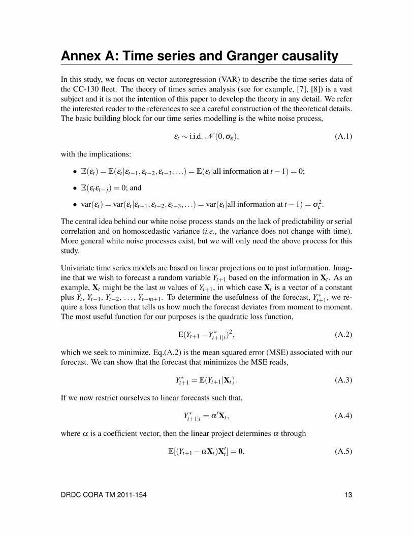
Annex A: Time series and Granger causality

In this study, we focus on vector autoregression (VAR) to describe the time series data of

the CC-130 fleet. The theory of times series analysis (see for example, [7], [8]) is a vast

subject and it is not the intention of this paper to develop the theory in any detail. We refer

the interested reader to the references to see a careful construction of the theoretical details.

The basic building block for our time series modelling is the white noise process,

εt ∼ i.i.d. N (0,σε), (A.1)

with the implications:

• E(εt) = E(εt |εt−1,εt−2,εt−3, . . .) = E(εt |all information at t−1) = 0;

• E(εtεt− j) = 0; and

• var(εt) = var(εt |εt−1,εt−2,εt−3, . . .) = var(εt |all information at t−1) = σ2ε .

The central idea behind our white noise process stands on the lack of predictability or serial

correlation and on homoscedastic variance (i.e., the variance does not change with time).

More general white noise processes exist, but we will only need the above process for this

study.

Univariate time series models are based on linear projections on to past information. Imag-

ine that we wish to forecast a random variable Yt+1 based on the information in Xt . As an

example, Xt might be the last m values of Yt+1, in which case Xt is a vector of a constant

plus Yt , Yt−1, Yt−2, . . . , Yt−m+1. To determine the usefulness of the forecast, Y ∗t+1, we re-

quire a loss function that tells us how much the forecast deviates from moment to moment.

The most useful function for our purposes is the quadratic loss function,

E(Yt+1−Y ∗t+1|t)2, (A.2)

which we seek to minimize. Eq.(A.2) is the mean squared error (MSE) associated with our

forecast. We can show that the forecast that minimizes the MSE reads,

Y ∗t+1 = E(Yt+1|Xt). (A.3)

If we now restrict ourselves to linear forecasts such that,

Y ∗t+1|t = α ′Xt , (A.4)

where α is a coefficient vector, then the linear project determines α through

E[(Yt+1−αXt)X′t ] = 0. (A.5)


DraftCopy

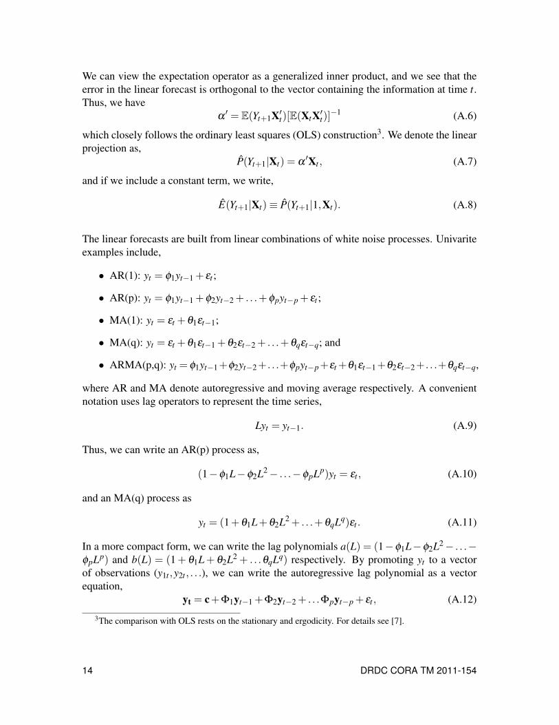
We can view the expectation operator as a generalized inner product, and we see that the

error in the linear forecast is orthogonal to the vector containing the information at time t.Thus, we have

α ′ = E(Yt+1X′t)[E(XtX′t)]−1 (A.6)

which closely follows the ordinary least squares (OLS) construction3. We denote the linear

projection as,

P(Yt+1|Xt) = α ′Xt , (A.7)

and if we include a constant term, we write,

E(Yt+1|Xt)≡ P(Yt+1|1,Xt). (A.8)

The linear forecasts are built from linear combinations of white noise processes. Univarite

examples include,

• AR(1): yt = φ1yt−1+ εt ;

• AR(p): yt = φ1yt−1+φ2yt−2+ . . .+φpyt−p + εt ;

• MA(1): yt = εt +θ1εt−1;

• MA(q): yt = εt +θ1εt−1+θ2εt−2+ . . .+θqεt−q; and

• ARMA(p,q): yt = φ1yt−1+φ2yt−2+. . .+φpyt−p+εt +θ1εt−1+θ2εt−2+. . .+θqεt−q,

where AR and MA denote autoregressive and moving average respectively. A convenient

notation uses lag operators to represent the time series,

Lyt = yt−1. (A.9)

Thus, we can write an AR(p) process as,

(1−φ1L−φ2L2− . . .−φpLp)yt = εt , (A.10)

and an MA(q) process as

yt = (1+θ1L+θ2L2+ . . .+θqLq)εt . (A.11)

In a more compact form, we can write the lag polynomials a(L) = (1−φ1L−φ2L2− . . .−φpLp) and b(L) = (1+ θ1L+ θ2L2 + . . .θqLq) respectively. By promoting yt to a vector

of observations (y1t ,y2t , . . .), we can write the autoregressive lag polynomial as a vector

equation,

yt = c+Φ1yt−1+Φ2yt−2+ . . .Φpyt−p + εt , (A.12)

3The comparison with OLS rests on the stationary and ergodicity. For details see [7].


DraftCopy

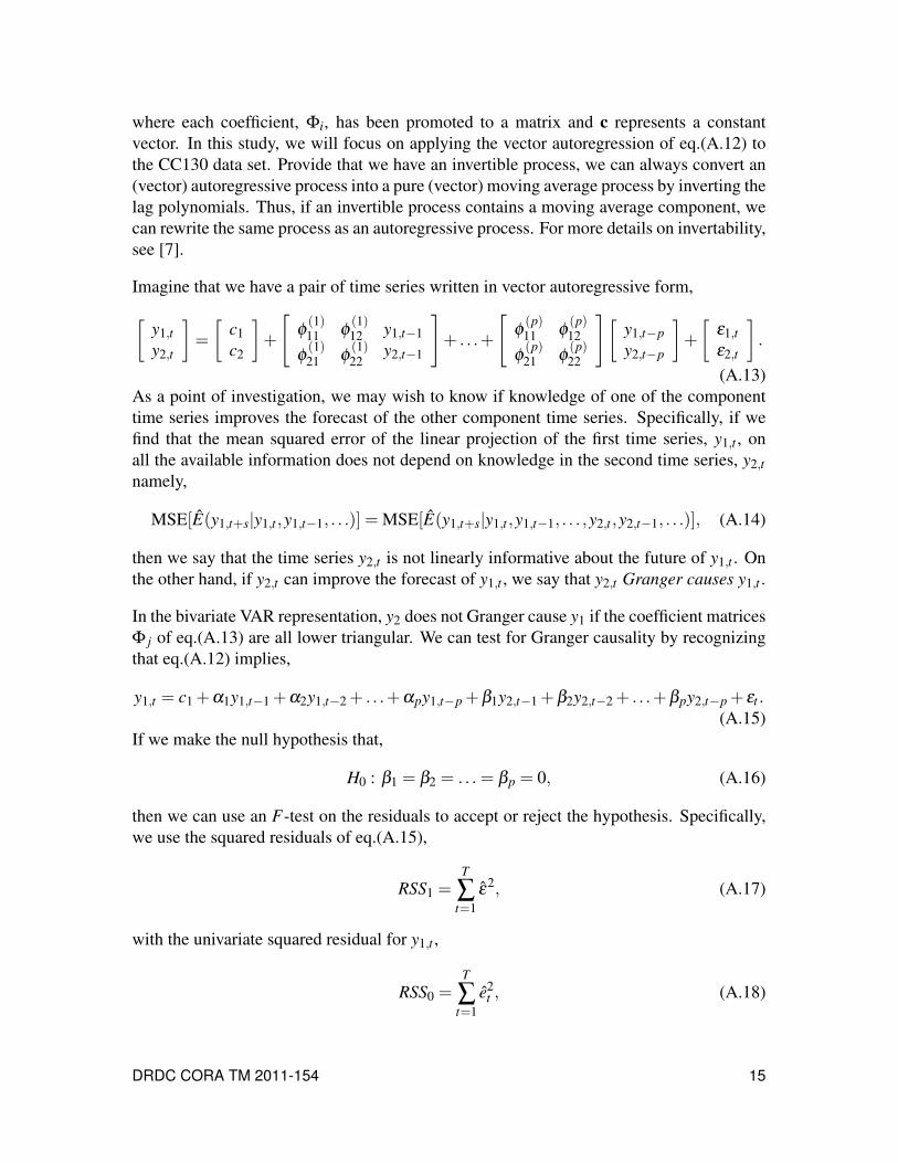
where each coefficient, Φi, has been promoted to a matrix and c represents a constant

vector. In this study, we will focus on applying the vector autoregression of eq.(A.12) to

the CC130 data set. Provide that we have an invertible process, we can always convert an

(vector) autoregressive process into a pure (vector) moving average process by inverting the

lag polynomials. Thus, if an invertible process contains a moving average component, we

can rewrite the same process as an autoregressive process. For more details on invertability,

see [7].

Imagine that we have a pair of time series written in vector autoregressive form,

[y1,ty2,t

]=

[c1c2

]+

[φ (1)11 φ (1)

12

φ (1)21 φ (1)

22

y1,t−1

y2,t−1

]+ . . .+

[φ (p)11 φ (p)

12

φ (p)21 φ (p)

22

][y1,t−py2,t−p

]+

[ε1,tε2,t

].

(A.13)

As a point of investigation, we may wish to know if knowledge of one of the component

time series improves the forecast of the other component time series. Specifically, if we

find that the mean squared error of the linear projection of the first time series, y1,t , onall the available information does not depend on knowledge in the second time series, y2,tnamely,

MSE[E(y1,t+s|y1,t ,y1,t−1, . . .)] =MSE[E(y1,t+s|y1,t ,y1,t−1, . . . ,y2,t ,y2,t−1, . . .)], (A.14)

then we say that the time series y2,t is not linearly informative about the future of y1,t . On

the other hand, if y2,t can improve the forecast of y1,t , we say that y2,t Granger causes y1,t .

In the bivariate VAR representation, y2 does not Granger cause y1 if the coefficient matrices

Φ j of eq.(A.13) are all lower triangular. We can test for Granger causality by recognizing

that eq.(A.12) implies,

y1,t = c1+α1y1,t−1+α2y1,t−2+ . . .+αpy1,t−p +β1y2,t−1+β2y2,t−2+ . . .+βpy2,t−p + εt .(A.15)

If we make the null hypothesis that,

H0 : β1 = β2 = . . .= βp = 0, (A.16)

then we can use an F-test on the residuals to accept or reject the hypothesis. Specifically,

we use the squared residuals of eq.(A.15),

RSS1 =T

∑t=1

ε2, (A.17)

with the univariate squared residual for y1,t ,

RSS0 =T

∑t=1

e2t , (A.18)


DraftCopy

where

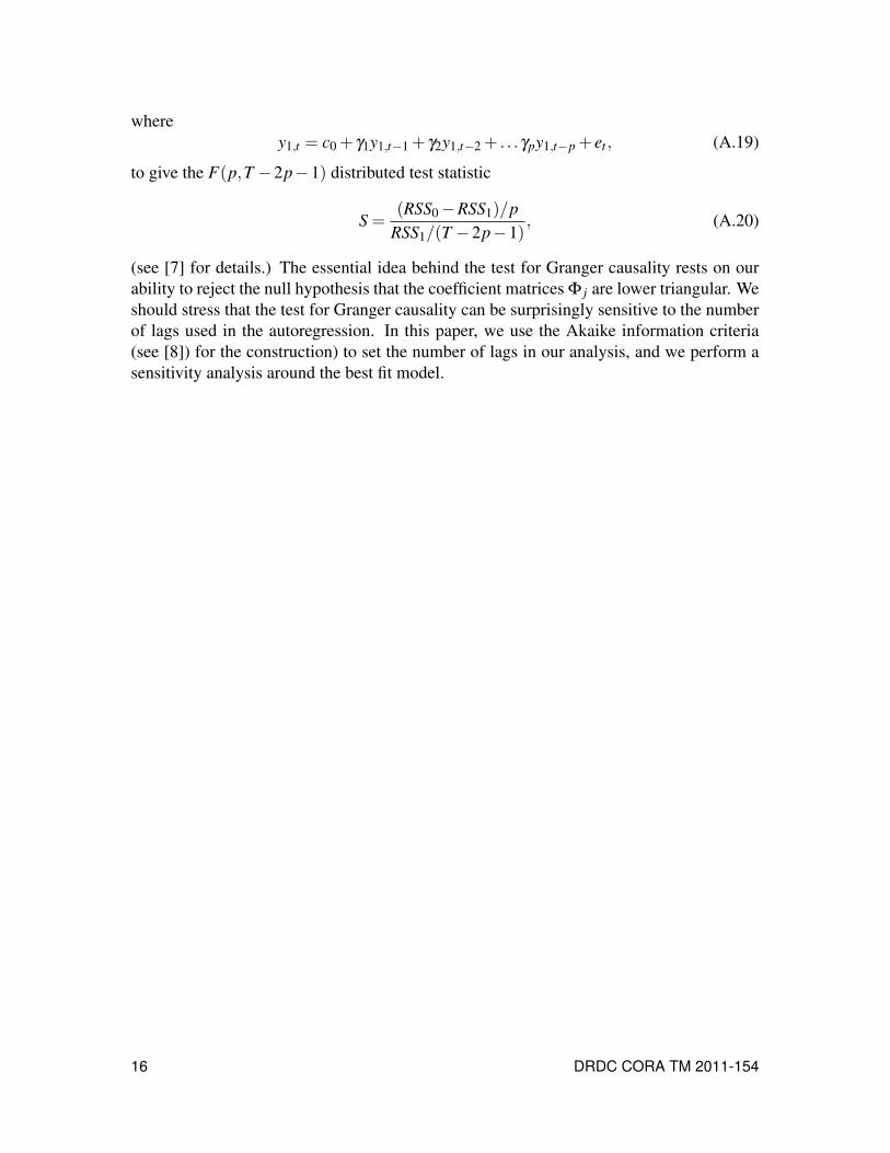
y1,t = c0+ γ1y1,t−1+ γ2y1,t−2+ . . .γpy1,t−p + et , (A.19)

to give the F(p,T −2p−1) distributed test statistic

S =(RSS0−RSS1)/p

RSS1/(T −2p−1), (A.20)

(see [7] for details.) The essential idea behind the test for Granger causality rests on our

ability to reject the null hypothesis that the coefficient matrices Φ j are lower triangular. We

should stress that the test for Granger causality can be surprisingly sensitive to the number

of lags used in the autoregression. In this paper, we use the Akaike information criteria

(see [8]) for the construction) to set the number of lags in our analysis, and we perform a

sensitivity analysis around the best fit model.


DraftCopy

Annex B: Fleet indicator definitions

This Annex contains the definitions of the fleet indicators used in the analysis provided in

this paper. The definitions listed below are taken verbatim from the PERFORMA database.

Further technical information can be found in the PERFORMA database[4].

All Failures

Definition: All Failures are the sum of the On-A/C Failures and the Off-A/C Failures.

• On-A/C Failures: Total number of failures recorded on a CF 349 form against a

piece of equipment installed on an Aircraft. Those are determined from all entries

recorded on the On-A/C CF 349 maintenance forms against any valid WUC, where

the equipment had to be replaced or repaired in order to return the Aircraft to a

serviceable status. This includes all valid Sequence 1 and 2 line entries.

• Off-A/C Failures: Total number of failures recorded against uninstalled equipment.

An Off-A/C form is defined as a CF 349 formwithout an Aircraft number or a CF 543

form. A failure will have a Fix = 3 or for non-serialized items, the Fix = 6 with a con-

tractor Fixer Unit Code (3 letters) and a supplementary data of TLRO/TLIR/TLM.

Ao – Operational Availability as % of time

Definition: (Ao) Operational Availability as % of time is the proportion of observed time

that a group of Aircraft is in an operable state (not undergoing maintenance) in relation

to the total operational time available during a stated period. Operational Availability as

percentage of time is calculated using: Ao = Up Time / (Up Time + Down Time) Where:

“Up Time” is the total actual number of calendar hours where the selected Aircraft are

not undergoing any maintenance action during the chosen period (no open CF 349) and

the Allocation Code is not “LX”. And: “Up Time + Down Time” is the total number of

calendar hours included in the selected period of the analysis. In calculating all downtimes

and uptimes, the date and time are translated to the nearest hour based on 24/7 operations.

Corrective Maintenance Person-Hours Rate

Definition: Total number of “Maintenance Person-Hours” reported on CF 349 and CF

543 corrective maintenance forms for every 1000 hours flown by a specific fleet. This

calculation involves three defaults when examining MPHRs for a particular component.

• Installation Factor (IF): Quantity of the same item that is installed on a single Aircraft

(e.g. there are two engines on the Aircraft). The Installation Factor information is

not available so 1 is used as default.


DraftCopy

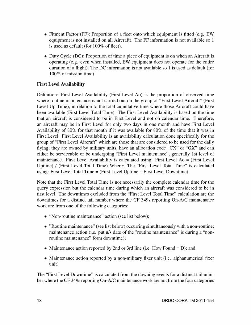
• Fitment Factor (FF): Proportion of a fleet onto which equipment is fitted (e.g. EW

equipment is not installed on all Aircraft). The FF information is not available so 1

is used as default (for 100% of fleet).

• Duty Cycle (DC): Proportion of time a piece of equipment is on when an Aircraft is

operating (e.g. even when installed, EW equipment does not operate for the entire

duration of a flight). The DC information is not available so 1 is used as default (for

100% of mission time).

First Level Availability

Definition: First Level Availability (First Level Ao) is the proportion of observed time

where routine maintenance is not carried out on the group of “First Level Aircraft” (First

Level Up Time), in relation to the total cumulative time where those Aircraft could have

been available (First Level Total Time). The First Level Availability is based on the time

that an aircraft is considered to be in First Level and not on calendar time. Therefore,

an aircraft may be in First Level for only two days in one month and have First Level

Availability of 80% for that month if it was available for 80% of the time that it was in

First Level. First Level Availability is an availability calculation done specifically for the

group of “First Level Aircraft” which are those that are considered to be used for the daily

flying; they are owned by military units, have an allocation code “CX” or “GX” and can

either be serviceable or be undergoing “First Level maintenance”, generally 1st level of

maintenance. First Level Availability is calculated using: First Level Ao = (First Level

Uptime) / (First Level Total Time) Where: The “First Level Total Time” is calculated

using: First Level Total Time = (First Level Uptime + First Level Downtime)

Note that the First Level Total Time is not necessarily the complete calendar time for the

query expression but the calendar time during which an aircraft was considered to be in

first level. The downtimes excluded from the “First Level Total Time” calculation are the

downtimes for a distinct tail number where the CF 349s reporting On-A/C maintenance

work are from one of the following categories:

• “Non-routine maintenance” action (see list below);

• ”Routine maintenance” (see list below) occurring simultaneously with a non-routine;

maintenance action (i.e. put u/s date of the "routine maintenance" is during a “non-

routine maintenance” form downtime);

• Maintenance action reported by 2nd or 3rd line (i.e. How Found = D); and

• Maintenance action reported by a non-military fixer unit (i.e. alphanumerical fixer

unit)

The “First Level Downtime” is calculated from the downing events for a distinct tail num-

ber where the CF 349s reporting On-A/Cmaintenance work are not from the four categories


DraftCopy

listed above. The downtimes for all these downing events are calculated for each distinct

tail number and added up to get the total “First Level Downtime”. A downing event down-

time is composed of a single or a group of CF 349s reporting work performed On-A/C

(i.e. CF 349s must have a tail number) from the time the Aircraft was first put u/s to the

completion of the maintenance work that brings the Aircraft to a serviceable status. The

downtime calculation for any downing event starts when a CF 349 form is opened against a

distinct tail number (put u/s date-time when the Aircraft becomes unserviceable) and ends

when the last CF 349 is closed ’ (last certified serviceable date-time bringing the Aircraft

back to a serviceable status) The “First Level Up Time” is defined as any period where a

First Level Aircraft is not undergoing maintenance.

Flying Hours

Definition: Total flying hours recorded by the aircrew during a given time period as re-

ported via the monthly AUSR report.

Mean Flying Time Between On-A/C Corrective Forms

Definition: Average elapsed flying time between two consecutive On-A/C Corrective Forms.

This is determined by dividing the total operating hours of a piece of equipment over a

given period by the total number of On-A/C Corrective Forms recorded against that equip-

ment. For periods with no forms or events occurring, the operating hours will be shown.

Mean Flying Time Between On-A/C Preventive Forms

Definition: Average elapsed flying time between two consecutive On-A/C Preventive Forms.

This is determined by dividing the total operating hours of a piece of equipment over a

given period by the total number of On-A/C Preventive Forms recorded against that equip-

ment. For periods with no forms or events occurring, the operating hours will be shown.

This parameter is more suitable for analysis at the system or component level.

Mean Flying Time Between Downing Events

Definition: MFTBDE indicates the average flying hours between two consecutive Aircraft

Downing Events. A downing event refers to any single occurrence, or group of occur-

rences, where an Aircraft is brought from a Serviceable/Operational status to an Unser-

viceable/Repair status. These include both Preventive and Corrective Maintenance Actions

reported against an operational Aircraft. Only forms with a numerical fixer unit are in-

cluded in an event. A downing event may include several failures that are all repaired

following the single downing event.

Off-A/C Maintenance Person-Hours Rate

Definition: Total number of “Maintenance Person-Hours” reported on “Off-A/C” forms for

every 1000 hours flown by a specific fleet or selected Aircraft.


DraftCopy

This calculation involves three defaults when examining MPHRs for a particular compo-

nent.











On-A/C Maintenance Person-Hours Rate

Definition: Total number of “Maintenance Person-Hours” reported on “On-A/C” forms for

every 1000 hours flown by a specific fleet or selected Aircraft.

This calculation involves three defaults when examining MPHRs for a particular compo-

nent.











On Aircraft Robs Maintenance Person-Hour Rate

Definition: Number of “Maintenance Person-Hours” reported against a ROB on “On-A/C

forms” for every 1000 hours flown by a specific fleet or selected Aircraft. This calculation

involves three defaults when examining MPHRs for a particular component.





DraftCopy








Ops Mission Aborts Rate

Definition: Total number of “Ops Mission Aborts” reported for every 1000 hours flown by

a specific fleet.

Rate calculations involve three defaults.











Preventive Maintenance Person-Hours Rate

Definition: Total number of “Maintenance Person-Hours” reported on CF 349 and CF

543 preventive maintenance forms for every 1000 hours flown by a specific fleet. This

calculation involves three defaults when examining MPHRs for a particular component.












DraftCopy

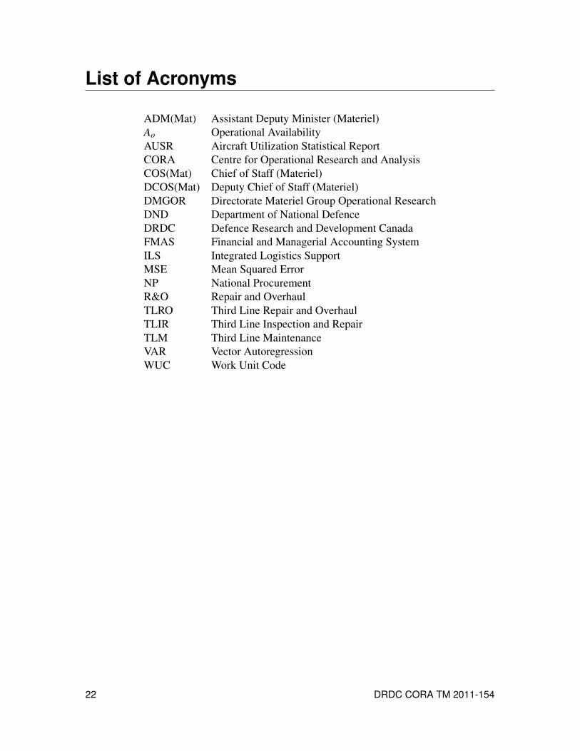
List of Acronyms

ADM(Mat) Assistant Deputy Minister (Materiel)

Ao Operational Availability

AUSR Aircraft Utilization Statistical Report

CORA Centre for Operational Research and Analysis

COS(Mat) Chief of Staff (Materiel)

DCOS(Mat) Deputy Chief of Staff (Materiel)

DMGOR Directorate Materiel Group Operational Research

DND Department of National Defence

DRDC Defence Research and Development Canada

FMAS Financial and Managerial Accounting System

ILS Integrated Logistics Support

MSE Mean Squared Error

NP National Procurement

R&O Repair and Overhaul

TLRO Third Line Repair and Overhaul

TLIR Third Line Inspection and Repair

TLM Third Line Maintenance

VAR Vector Autoregression

WUC Work Unit Code


DraftCopy

DOCUMENT CONTROL DATA(Security classification of title, body of abstract and indexing annotation must be entered when document is classified)

1. ORIGINATOR (The name and address of the organization preparing thedocument. Organizations for whom the document was prepared, e.g. Centresponsoring a contractor’s report, or tasking agency, are entered in section 8.)

Defence R&D Canada – CORADept. of National Defence, MGen G.R. Pearkes Bldg.,101 Colonel By Drive, Ottawa, Ontario, Canada K1A0K2

2. SECURITY CLASSIFICATION (Overallsecurity classification of the documentincluding special warning terms if applicable.)

UNCLASSIFIED

3. TITLE (The complete document title as indicated on the title page. Its classification should be indicated by the appropriateabbreviation (S, C or U) in parentheses after the title.)

Granger Causality and National Procurement Spending

4. AUTHORS (Last name, followed by initials – ranks, titles, etc. not to be used.)

Maybury, D.W.

5. DATE OF PUBLICATION (Month and year of publication ofdocument.)

September 2011

6a. NO. OF PAGES (Totalcontaining information.Include Annexes,Appendices, etc.)

32

6b. NO. OF REFS (Totalcited in document.)

8

7. DESCRIPTIVE NOTES (The category of the document, e.g. technical report, technical note or memorandum. If appropriate, enterthe type of report, e.g. interim, progress, summary, annual or final. Give the inclusive dates when a specific reporting period iscovered.)

Technical Memorandum

8. SPONSORING ACTIVITY (The name of the department project office or laboratory sponsoring the research and development –include address.)

Defence R&D Canada – CORADept. of National Defence, MGen G.R. Pearkes Bldg., 101 Colonel By Drive, Ottawa, Ontario,Canada K1A 0K2

9a. PROJECT NO. (The applicable research and developmentproject number under which the document was written.Please specify whether project or grant.)

N/A

9b. GRANT OR CONTRACT NO. (If appropriate, the applicablenumber under which the document was written.)

10a. ORIGINATOR’S DOCUMENT NUMBER (The officialdocument number by which the document is identified by theoriginating activity. This number must be unique to thisdocument.)

DRDC CORA TM 2011-154

10b. OTHER DOCUMENT NO(s). (Any other numbers which maybe assigned this document either by the originator or by thesponsor.)

11. DOCUMENT AVAILABILITY (Any limitations on further dissemination of the document, other than those imposed by securityclassification.)( X ) Unlimited distribution( ) Defence departments and defence contractors; further distribution only as approved( ) Defence departments and Canadian defence contractors; further distribution only as approved( ) Government departments and agencies; further distribution only as approved( ) Defence departments; further distribution only as approved( ) Other (please specify):

12. DOCUMENT ANNOUNCEMENT (Any limitation to the bibliographic announcement of this document. This will normally correspondto the Document Availability (11). However, where further distribution (beyond the audience specified in (11)) is possible, a widerannouncement audience may be selected.)

DraftCopy

13. ABSTRACT (A brief and factual summary of the document. It may also appear elsewhere in the body of the document itself. It is highlydesirable that the abstract of classified documents be unclassified. Each paragraph of the abstract shall begin with an indication of thesecurity classification of the information in the paragraph (unless the document itself is unclassified) represented as (S), (C), (R), or (U).It is not necessary to include here abstracts in both official languages unless the text is bilingual.)

Using Granger causality tests, we look for relationships in performance and National Procure-ment spending time series data that can improve forecasting capabilities with the CC130 fleet.We find that no meaningful relationships exist between spending and performance indicatorswithin the spending envelope studied. Our results concord with earlier work based on randommatrix theory and minimal spanning trees, which suggest the fleet is robust to spending shocks.We conclude that NP spending changes do not correlate with subsequent CC130 Hercules air-craft performance changes and vice versa. Granger causality tests represent a powerful toolwhich can be used with future fleet studies.

14. KEYWORDS, DESCRIPTORS or IDENTIFIERS (Technically meaningful terms or short phrases that characterize a document and couldbe helpful in cataloguing the document. They should be selected so that no security classification is required. Identifiers, such asequipment model designation, trade name, military project code name, geographic location may also be included. If possible keywordsshould be selected from a published thesaurus. e.g. Thesaurus of Engineering and Scientific Terms (TEST) and that thesaurus identified.If it is not possible to select indexing terms which are Unclassified, the classification of each should be indicated as with the title.)

Granger causalityFleet performanceNational procurement spendingTime Series

DraftCopy

DraftCopy

DRDC CORA

www.drdc-rddc.gc.ca

granger causality and national procurement … spending time series data that can improve...

Documents