Grand Corruption by Theft and Bribery

Desiree A. Desierto∗

George Mason University

January 13, 2021

Abstract

A public official who has discretionary power over the government budget can ob-tain rents by stealing government revenues or receiving bribe payments in exchangefor spending those revenues on public goods and services. I propose a method of si-multaneously measuring these two kinds of grand corruption. I then demonstrate itusing data from asset declarations of municipal mayors in the Philippines. The resultssuggest that an increase in government revenues increases theft, but decreases bribesby a larger extent such that total corruption falls. However, public good provision alsodeclines since some of the additional revenues are stolen.

∗Email: ddesiert@gmu.edu; Address: Economics Department, George Mason University, Buchanan Hall,1st Floor, MSN 3G4, Fairfax VA 22030. I am grateful for comments from, and discussions with, ScottGehlbach, Rikhil Bhavnani, Teppei Yamamoto, David Weimer, John Duggan, Mark Koyama, Nathan Nunn,Cesar Martinelli, and seminar audiences at Stanford, Wisconsin, George Mason, Tulane, Kentucky, Illinois,Rochester, and American University.

1 Introduction

This paper is the first to simultaneously measure two kinds of grand corruption: the theft of

government revenues, and bribe payments from public spending. Both types of corruption

are ubiquitous, especially in the developing world.1 Two of the largest corruption scandals to

date illustrate how government revenues can be siphoned off directly, or otherwise allocated

to public projects that are implemented by firms from which public officials obtain bribes

and kickbacks. Former Malaysian Prime Minister Najib Razak is currently on trial for his

suspected involvement in the theft of over $4.5 billion from the Malaysia’s state development

fund 1MDB, out of which $681 million were allegedly transferred to Mr. Razak’s personal

bank account. The funds were apparently embezzled out of the country and spent on luxury

properties, yachts, and even used to fund the 2013 Hollywood film “The Wolf of Wall Street”.

In Brazil, the Petrobras scandal illustrates large scale corruption in the form of bribery,

in which officials at the state-owned oil company Petroleo Brasileiro were alleged to have

received bribes from construction companies in exchange for awarding contracts to the latter.

The scandal is estimated to have amounted to $9.5 billion in illicit payments, some of which

were alleged to have been used in vote-buying schemes that benefited the Workers Party,

including former Presidents Ignacio Lula Da Silva and Dilma Rousseff.

The costs are enormous even in normal times. The OECD (2013) estimates that about

20 to 25% of government procurement budgets, equivalent to about $2 trillion or 2% of

global GDP, are lost annually to corruption, while the IMF (2017) suggests that such an

amount captures the annual cost of bribery alone. The cost of theft is also likely to be large.

Global Financial Integrity (2015) calculates that between 2004 to 2013, developing countries

lost $ 7.8 trillion from illicit financial outflows due to trade misinvoicing and leakages in the

balance of payments. The Independent reports that about $1 trillion a year is siphoned away

1These, of course, are not the only types of grand corruption. From Transparency International: “Grandcorruption occurs when a public official...causes the State or any of its people a loss greater than 100 times theannual minimum subsistence income of its people; as a result of bribery, embezzlement or other corruption of-fence”. See https://www.transparency.org/news/feature/what is grand corruption and how can we stop it.For recent surveys, see Fisman and Golden (2017) and Rose-Ackerman and Palifka (2016).

1

from developing countries through money laundering, tax evasion, and embezzlement.2

Theft and bribery also occur at the local level – in some cases, local government officials

embezzle public funds that have already been allocated towards particular projects, while in

other cases, they allocate the funds towards projects in exchange for bribes and kickbacks.

For instance, Olken (2006) shows that in Indonesia, about 18% of government subsidized

rice that were allocated to villages and districts ‘disappeared’ in that they were not received

by the intended households. Olken suggests that the rice was stolen by village officials who

were in charge of distributing it. Similarly, Reinikka and Svensson (2004) show that 86%

of Uganda’s educational grants were not received by schools, while Neihaus and Suktankhar

(2013) estimate that 79% of funds allocated to India’s National Rural Employee Guarantee

Scheme did not reach the employees. Meanwhile, Batalla (2000) provides anecdotal evidence

of how bribery from public spending occurs at the local level in the Philippines. Large

public works projects that cover multiple jurisdictions are divided into smaller projects so

that local governments could award them to their ‘favored’ contractors. In exchange, local

officials apparently earn kickbacks amounting to about 20 to 40% of the project. More recent

evidence of local-level bribery in developing countries include Knutsen, Kotsadam, Olsen,

and Wig (2016) for Africa, Brierley (2020) for Ghana, and Figueroa (2020) for Argentina.

Developed countries are not immune to such instances of corruption. Dincer and Johnston

(2018) provide a corruption perceptions index for states in the U.S. and reveal that in most

states, illegal corruption in the state’s executive and legislative branches are perceived to be

“slightly common” or “moderately common”. Leeson and Sobel (2008) analyze a specific

type of public good provision from which local public officials can steal revenues or earn bribes

- the allocation of funds for disaster relief. They show that between 1990 and 1999, each

$100 of funds provided by the Federal Emergency Management Agency (FEMA) to states

for natural disaster relief increased the state’s average number of convictions of corruption-

related crimes by 102%. They suggest two ways by which state public officials benefit - theft

2See http://www.independent.co.uk/news/world/politics/criminals-and-corrupt-politicians-steal-1trn-a-year-from-the-worlds-poorest-countries-9707104.html.

2

and bribery. Citing Lakin (2004), they note that officials in Buchanan county in Virginia

solicited bribes from firms that have been awarded contracts for reconstruction projects. As

an example of theft, they mention that in 2005, a public employee in Florida attempted to

embezzle $48,000 of FEMA relief after a hurricane in 1998.

The key distinction between theft and bribery is that theft is directly appropriated from

revenues, whereas bribes are indirectly earned by spending those revenues. One could then

estimate the direct effect of government revenues on a public official’s accumulated wealth

to measure her accumulated rents from theft, and estimate the indirect effect of revenues

through public spending to measure her accumulated rents from bribes. The problem, how-

ever, is that these two effects cannot be readily measured because of a critical simultaneity

problem: the revenues that are stolen cannot be spent. This means that the public official’s

accumulated rents and the level of public spending are jointly determined. Unless one im-

poses additional restrictions, it is impossible to measure both the direct and the indirect

effects of government revenues.

To obtain such restrictions, I construct a formal model from which I derive an important

comparative static result that enables one to separate out the direct from the indirect effect.

I find that there exists a threshold level of government revenues, at and below which the

public official is constrained not to steal revenues and, therefore, can only keep increasing

her rents by spending each additional revenue and extracting bribes therefrom. Above the

threshold, I find that each additional revenue is stolen, which implies that public spending

above the threshold, and the amount of bribes associated with it, remain fixed. To estimate

the direct effect, one could then use data from jurisdictions that have revenues above the

threshold. Pinning down the direct effect, one could then use data from jurisdictions below

and above the threshold to estimate the indirect effect since bribe-taking occurs below and

above the threshold, albeit at a fixed rate in the latter region.

To implement the statistical procedure, I parameterize the model, add stochastic errors,

make additional assumptions, and derive the formulae for the direct effect and the indirect

3

effect. I then propose a two-step estimation of the parameters in the formulae. First, given

data on many jurisdictions, one estimates the probability that a jurisdiction is at or below

the threshold level of revenues. Second, one estimates the model’s parameters using the

subset of jurisdictions at or below the threshold, and the subset of jurisdictions above the

threshold. These estimated parameters, along with the estimated probability from the first

step, are finally combined according to the formulae for the direct and indirect effects.

Finally, to illustrate the method, I use data from municipalities in the Philippines. The

Philippines is an ideal test case, since instances of grand corruption in the allocation of

public funds abound, both in the form of theft and bribery. Anecdotal evidence suggest that

between 20 to 40% of the cost of road construction projects are routinely spent on public

officials as bribes and kickbacks (See Batalla, 2000). Theft also appears to be rampant. In

fact, between 1979 to 2016, over 10,000, or almost 30% of all corruption cases filed against

high-level public officials were cases involving the malversation of public funds.3

Another advantage to using Philippine data is that the municipal mayor’s rents can

be directly quantified using asset declarations—the Statement of Assets, Liabilities, and

Net Worth (SALN), which all public employees and elected officials are required to submit

for each year in office. While, in principle, data from SALNs can be accessed by private

individuals, large-scale statistical analyses of the reported assets in the SALNs have not

been done before, and understandably so, since only hard (paper) copies of the SALNs can

be requested from the government repository. Thus, for this study, I manually collected,

digitized, and encoded the data from all the SALNs submitted by mayors in multiple years.4

3The figures are based on the following article in Philippine news network Rappler that reports onthe number of corruption cases filed in the Sandiganbayan: https://www.rappler.com/newsbreak/159148-biggest-corruption-cases-sandiganbayan-graft-plunder-malversation. The Sandiganbayan is a special court,established in 1978 by Presidential Decree (PD) No. 1486, which has jurisdiction over all cases involving high-level public officials in the exercise of their duties. Malversation of public funds involves the appropriation ofpublic funds by a public official who is accountable for such funds. (See the Philippine Revised Penal Code(Title VII, Ch. 4, Art. 217) for the complete legal definition).

4Asset disclosure statements have been used to identify the rents from public office in other countries.In particular, Eggers and Hainmueller (2011) and Ziobrowski et al. (2011), among others, use the FinancialDisclosure Reports of members of the US Congress to estimate the value of holding public office in the US.Meanwhile, Fisman et al. (2014) use disclosure affidavits of candidates in state assembly elections in Indiato compute the difference in the change in the net worth of election winners and losers.

4

As a proxy for the public official’s accumulated wealth, I compute the growth of a municipal

mayor’s assets during one term of office, while dealing with issues of selection and likely

misreporting in the SALN.

I find a positive direct effect and a negative indirect effect. That is, municipal revenues in-

crease a mayor’s accumulated rents from theft, but decrease accumulated rents from bribery.

The estimated magnitude of the indirect effect is larger than that of the direct effect, such

that the net change in total accumulated rents is negative. This suggests that in the case

of the Philippines, an increase in government revenues lowers corruption, in that total rent

accumulation slows down, but it also decreases the provision of public goods and services

since some of the additional revenues are stolen.

One might contend that only the change in total rents should matter, and that the source

of such rents – whether theft or bribery is irrelevant. I offer three arguments to rebut this

claim. First, anti-corruption efforts may be more effective when it can target the exact

nature of the corrupt act. In the Philippines, for example, a public official who engages in

the theft of government revenues may be charged with crimes of graft and malversation of

public funds, in which case, the documentation of irregular transactions, e.g. audits, may be

sufficient evidence.5 On the other hand, bribery charges require stronger evidence since the

receipt of rents alone does not establish that bribery has taken place—to prove that there

was a quid pro quo arrangement, it also has to be shown that the rents were obtained in

exchange for a specific favor.

Second, the type of high-level corruption that occurs has important implications on social

welfare. While theft involves a dollar-for-dollar transfer of revenues from tax payers to the

public official, bribes are paid in exchange for public goods whose marginal social benefit

may be large. Thus, even when additional revenues decrease total rents, net social welfare

may decrease if the foregone marginal bribe payments are sufficiently large, since the latter

also implies a significant loss of marginal social benefit from the additional public goods that

5Avis, Ferraz and Finan (2018) show the effectiveness of random audits in Brazil.

5

could have been provided had the public official taken the extra bribes instead.

Lastly, this analysis has implications on political turnover. If bribes are associated with

some positive social benefit, citizens might be willing to condone incidents of bribery. In-

deed, recent papers suggest that in selecting political leaders, voters in developing coun-

tries knowingly make a tradeoff between corruption and competence (see, e.g. Rosas and

Manzetti (2015), Choi and Woo (2013), Zechmeister and Zizumbo-Colunga (2013). Winters

and Weitz-Shapiro (2013) sum up this idea of a tradeoff using the Portuguese “rouba, mas

faz”—“He robs, but he gets things done”). In contrast, the theft of government revenues

presents no such tradeoff, precisely because stolen public funds cannot therefore be spent

on public goods and services. Thus, voters might be less willing to tolerate the rent-seeking

behavior of an official who steals public funds, and are thus less likely to select such official,

than one who obtains rents from bribe payments alone.

2 Theft and Bribery in Public Good Provision

Grossman and Helpman (2001) provide a model of public good provision by a public official

who extracts bribes from the private sector in exchange for spending government revenues

on public goods. In this extension, I allow for the possibility that the official also steals some

of the revenues.

Consider a jurisdiction with two sectors/principals whose common agent – a public official

in charge of the government budget, decides how to use government revenues T . Specifically,

the agent allocates public spending g1 towards principal 1 and g2 to principal 2. Principal 1

offers the agent bribe b in exchange for g1, and derives net benefit V (g1)− b from spending.

(Principal 2 does not offer bribes and derives benefit V (g2) from spending.) Let V ′(·) >

0, V ′′(·) < 0.

Faced with the bribe offer, the agent then chooses (g1, g2), and keeps any unspent revenues

for herself. The agent’s total rents R thus consist of stolen revenues and the bribe payment,

6

i.e. R = T − g1 − g2 + b. The agent also cares about social welfare such that her utility is

given by U = λ[V (g1) + V (g2)] + (1− λ)(T − g1 − g2 + b), where λ ∈ (0, 1) is the weight she

attaches to social welfare.

As standard in common agency models with complete information, in equilibrium, the

agent’s action (spending allocation) and the principal’s payment (bribes) are jointly efficient.

The equilibrium allocation and bribe payment is thus a solution to the following problem:

maxg1,g2,b

V (g1)− b

s.t. λ[V (g1) + V (g2)] + (1− λ)(T − g1 − g2 + b) ≥ U (a)

g1 + g2 − T ≤ 0 (b),

where U is the agent’s reservation utility—what it would obtain if it rejects principal 1’s

offer. Thus, (a) is the agent’s participation constraint. Meanwhile, constraint (b) captures

the possibility of theft. If (b) holds with equality, i.e. the constraint is binding, then no

theft is possible; hence (b) is the ‘no-theft constraint’. If it is non-binding, the amount

T − g1 − g2 > 0 can be stolen.

Proposition 1 below formally establishes that there exists a threshold value of revenues

T , at or below which the no-theft constraint is binding and, therefore, theft is not possible.

This implies that T captures the demand for public spending that the agent is constrained

to meet. Above this threshold, the no-theft constraint is non-binding and, thus, the agent

can now steal. Because only public spending at the amount of T has to be met, the agent is

able to steal all additional revenues above T .

Thus, Proposition 1 shows that when the agent is constrained not to steal and has to

spend all the revenues, the equilibrium amounts of public spending, g∗1 and g∗2, depend on

the size of the revenues (as well as the weight λ attached to social welfare). In contrast, if

the agent is unconstrained not to steal and therefore steals all additional revenues above T ,

then g∗1 and g∗2 are independent of the size of the revenues and only depend on λ.

Total equilibrium rents R∗ are therefore equal to equilibrium bribes b∗ when the no-theft

7

constraint is binding, or when revenues are at or below T , since theft is not possible. (In

turn, b∗ is determined by the amount spent on the bribing sector, g∗1, as well as T and λ).

When the no-theft constraint is non-binding, or revenues are above T , then R∗ consists of

both the equilibrium amount of bribes b∗ and of stolen revenues T − g∗1 − g∗2.

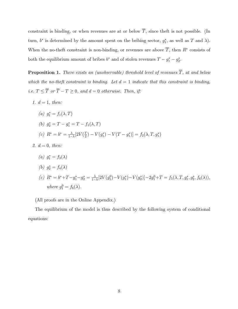
Proposition 1. There exists an (unobservable) threshold level of revenues T , at and below

which the no-theft constraint is binding. Let d = 1 indicate that this constraint is binding,

i.e. T ≤ T or T − T ≥ 0, and d = 0 otherwise. Then, if:

1. d = 1, then:

(a) g∗1 = f1(λ, T )

(b) g∗2 = T − g∗1 = T − f1(λ, T )

(c) R∗ = b∗ = λ1−λ [2V (T

2)− V (g∗1)− V (T − g∗1)] = f2(λ, T, g

∗1)

2. d = 0, then:

(a) g∗1 = f3(λ)

(b) g∗2 = f4(λ)

(c) R∗ = b∗+T−g∗1−g∗2 = λ1−λ [2V (g01)−V (g∗1)−V (g∗2)]−2g01+T = f5(λ, T, g

∗1, g∗2, f6(λ)),

where g01 = f6(λ).

(All proofs are in the Online Appendix.)

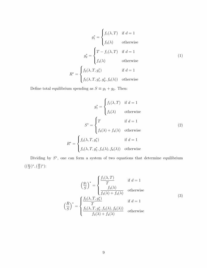
The equilibrium of the model is thus described by the following system of conditional

equations:

8

g∗1 =

f1(λ, T ) if d = 1

f3(λ) otherwise

g∗2 =

T − f1(λ, T ) if d = 1

f4(λ) otherwise

R∗ =

f2(λ, T, g

∗1) if d = 1

f5(λ, T, g∗1, g∗2, f6(λ)) otherwise

(1)

Define total equilibrium spending as S ≡ g1 + g2. Then:

g∗1 =

f1(λ, T ) if d = 1

f3(λ) otherwise

S∗ =

T if d = 1

f3(λ) + f4(λ) otherwise

R∗ =

f2(λ, T, g

∗1) if d = 1

f5(λ, T, g∗1, f4(λ), f6(λ)) otherwise

(2)

Dividing by S∗, one can form a system of two equations that determine equilibrium

((g1S

)∗, (RS

)∗):

(g1S

)∗=

f1(λ, T )

Tif d = 1

f3(λ)

f3(λ) + f4(λ)otherwise

(RS

)∗=

f2(λ, T, g

∗1)

Tif d = 1

f5(λ, T, g∗1, f4(λ), f6(λ))

f3(λ) + f4(λ)otherwise

(3)

9

This can be expressed more generally as:

(g1S

)∗=

h1(λ, T ) if d = 1

h2(λ) otherwise

(RS

)∗=

h3(λ, T, g

∗1) if d = 1

h4(λ, T, g∗1) otherwise

(4)

Lastly, note that while Proposition 1 establishes the existence of T , the model cannot

determine its value. Thus, while the amount of revenues T is observable, whether or not it

exceeds T , and therefore the indicator variable d, is unobservable. However, d depends on

revenues, since a larger T makes it more likely that it exceeds T . It also depends on λ, since

the agent is more constrained not to steal the more she cares about social welfare. That is:

Proposition 2. The value of d depends on λ and T .

3 Measuring Theft and Bribery

To take this model to the data, I parameterize (4) and include a vector of error terms u which

are necessary for two reasons. One is that there may be other variables that can possibly

affect g1S, RS

, and d. The other is that RS

and d are measured with error. Since rents are

inherently hidden, one cannot perfectly quantify R. Whether or not the no-theft constraint

is binding, i.e. d, is unobservable and can thus only be captured by a proxy variable.

Thus, let y = (g1S, RS

) and d be the dependent variables in the system, x = (1, λ, T )

the independent variables, u the error term, and θ a vector of parameters. Assume a finite

population of jurisdictions {Z}, with |Z| = Z. For jurisdiction i ∈ {Z}, the system can be

expressed as

g(yi, di,xi,ui|θ) = 0. (5)

10

Consider the following assumptions:

ASSUMPTIONS

1. There exists a unique solution for yi for every (xi, di,ui) such that yi = f(xi, di,ui|π),

where π is a vector of parameters that are functions of θ.

2. f is additively separable in (xi, di) and ui.

3. (a) E(ui|xi, di) = E(ui) and (b) ui ∼ N (0, σ2).

4. π = (α, β1, β2).

5. Pr(di = 1|xi) = Φ(xiα), where Φ is the standard normal cdf.

6. E(yi|xi, di = 1) = xiβ1 and E(yi|xi, di = 0) = xiβ

2.

Under assumptions 1 and 2, one can write equation (1) as:

yi = g(xi, di|π) + ui = E(yi|xi, di) + ui. (6)

Taking the expectation of E(yi|xi, di) over di:

yi = Pr(di = 1|xi)E(yi|xi, di = 1) + (1− Pr(di = 1|xi))E(yi|xi, di = 0) + ui, (7)

which, under assumptions 4, 5, and 6, can be written as:

yi = Φ(xiα)xiβ1 + (1− Φ(xiα))xiβ

2 + ui. (8)

Lastly, rearranging gives:

yi = xiγi + ui, (9)

where γi ≡ Φ(xiα)β1 + (1− Φ(xiα))β2.

11

3.1 Decomposing the Marginal Effect of Revenues on Total Rents

To identify the marginal rents from theft and those from bribery, one can conduct compara-

tive statics to determine the effect of T on RS

. Recall that total rents consist of stolen revenues

and bribe payments. Equation (4) implies that the total derivative of RS

with respect T is

(i)dRS

dT= ∂h3()

∂T+ ∂h3()

∂g1

∂g1∂T

if d = 1 and (ii)dRS

dT= ∂h4()

∂T+ ∂h4()

∂g1

∂g1∂T

= ∂h4()∂T

if d = 0. Thus, for a

jurisdiction with d = 1 such that theft cannot occur, a change in rents per total spending,

i.e. RS

, as a response to a change in T would be all due to a change in the amount of bribes

per total spending which, according to (i), operates through a change in g1. In contrast, for

a jurisdiction with d = 0 such that theft is possible, (ii) shows that there is no change in g1

as a response to a change in T . This implies that a change in T does not induce a change in

bribes per total spending and, thus, any change in RS

as a response to a change in T would

be due to a change in theft, or the amount of stolen revenues, per total spending.

The difficulty, however, is in identifying the overall, or average, change in theft and

bribery if some jurisdictions have d = 1 while others d = 0, given that d is endogenous to λ

and T . I thus derive these parameters.

To proceed, note that from (9), one can express the equation for RS i

as:

R

S i= γR0i + γRλiλi + γRTiTi + uRi , (10)

where:

γR0i = Φ(xiα)β1R0 + (1− Φ(xiα))β2

R0,

γRλi = Φ(xiα)β1Rλ + (1− Φ(xiα))β2

Rλ,

γRTi = Φ(xiα)β1RT + (1− Φ(xiα))β2

RT ,

β1 = [β1R0 β1

Rλ β1RT ] and β2 = [β2

R0 β2Rλ β2

RT ],

12

or:

R

S i= Φ(xiα)[(β1

R0 − β2R0) + (β1

Rλ − β2Rλ)λi + (β1

RT − β2RT )Ti] + β2

R0 + β2Rλλi + β2

RTTi + uRi .

By assumption 3, the expected value of RS i

given xi is:

E[(R

S i)|xi] = Φ(xiα)[(β1

R0−β2R0)+(β1

Rλ−β2Rλ)λi+(β1

RT−β2RT )Ti]+β

2R0+β2

Rλλi+β2RTTi. (11)

One can then obtain the derivative with respect to revenues:

dE[(RS i

)|xi]dTi

= [Φ(xiα)+φ(xiα)αTTi](β1RT−β2

RT )+φ(xiα)αT [(β1R0−β2

R0)+(β1Rλ−β2

Rλ)λi]+β2RT ,

(12)

where φ(xiα)αT is the marginal effect of Ti on Pr(d = 1)—with αT as the marginal effect of

Ti on the index function xiα and φ(·) the standard normal pdf.

Thus, for jurisdiction i ∈ {Z}, the total effect of revenues on its expected rents (per spend-

ing) is the sum of a direct effect (a) β2RT and an indirect effect (b) [Φ(xiα)+φ(xiα)αTTi](β

1RT−

β2RT ) + φ(xiα)αT [(β1

R0 − β2R0) + (β1

Rλ − β2Rλ)λi] through spending g1. That is, (a) is unaf-

fected by g1 whereas (b) is. To see this, note that by symmetry, one can get the following

expression:

dE[(g1S i

)|xi]dTi

= [Φ(xiα)+φ(xiα)αTTi](β1gT −β2

gT )+φ(xiα)αT [(β1g0−β2

g0)+(β1gλ−β2

gλ)λi]+β2gT

(13)

Re-writing this as Φ(xiα) + φ(xiα)αTTi =dE[(

g1S i

)|xi]dTi

−φ(xiα)αT [(β1g0−β2

g0)+(β1gλ−β

2gλ)λi]−β

2gT

β1gT−β

2gT

and

substituting into (13) obtain:

dE[(RS i

)|xi]dTi

=( dE[(

g1S i

)|xi]dTi

− φ(xiα)αT [(β1g0 − β2

g0) + (β1gλ − β2

gλ)λi]− β2gT

β1gT − β2

gT

)(β1

RT−β2RT )+β2

RT ,

(14)

where the first term is determined by spending, whereas the second term is not.

13

Thus, to summarize, the following are the population parameters of interest:

Definition The direct effect of jurisdiction i’s revenues, Ti, on its expected rents (per

spending), E[RS|xi], isD = β2

RT , while the indirect effect is Ii = [Φ(xiα)+φ(xiα)αTTi](β1RT−

β2RT ) + φ(xiα)αT [(β1

R0 − β2R0) + (β1

Rλ − β2Rλ)λi]. The total effect is the sum of the direct

and indirect effects, i.e. Wi = [Φ(xiα) + φ(xiα)αTTi](β1RT − β2

RT ) + φ(xiα)αT [(β1R0 − β2

R0) +

(β1Rλ − β2

Rλ)λi] + β2RT .

In turn, these parameters identify the marginal rents from theft, from bribery, and the

total change in corruption:

Proposition 3. Parameter D identifies the expected change in rents from theft (as a pro-

portion of total spending) in jurisdiction i as a response to a change in its revenues Ti,

parameter Ii the expected change in rents from bribes (as a proportion of total spending),

and parameter Wi the expected change in total rents (as a proportion of total spending).

3.2 Estimating the Direct, Indirect and Total Effects

The following two-step procedure obtains estimates for the direct effect (D), indirect effect

(Ii), and total effect (Wi) of revenues on the expected rents (per spending) in jurisdiction i,

using a random sample S ⊂ Z, with |S| = S.

1. Estimate Pr(di = 1)|xi) by probit regression to get αT and, for each municipality i in

sample S, Φi and φi.

2. Using the subset of the data for which di = 1, regress yi on xi by OLS to get β1. Do

the same for the subset for which di = 0 to get β2.

Using these estimates, one can then compute D, Ii, Wi according to the definition of the

population parameters D, Ii, Wi.

This procedure yields consistent estimates of D, Ii, Wi, under assumptions (5) and (6).

To see this, note that plim D = D, or plim β2RT = β2

RT since, under assumption (6), OLS

14

gives a consistent estimate of β2RT . As for the estimate of the indirect effect, note that under

assumption (6), OLS gives consistent estimates of β1RT , β

2RT , while under assumption (5),

the probit (MLE) regression gives consistent estimates of α and, hence, of Φ(·) and φ(·).

Thus, plim Ii = Ii, or plim[Φ(xiα) + φ(xiα)αTTi](β1RT − β2

RT ) + φ(xiα)αT [(β1R0 − β2

R0) +

(β1Rλ− β2

Rλ)λi] = [Φ(xiα)+φ(xiα)αTTi](β1RT −β2

RT )+φ(xiα)αT [(β1R0−β2

R0)+(β1Rλ−β2

Rλ)λi].

Finally, it follows that plim Wi ≡ Di + Ii = Di + Ii ≡ Wi.

Note that while D is the same for any i, the indirect effect Ii varies across i.6 One can also

summarize across sample S by taking the respective averages S−1ΣIi and S−1ΣWi. These

are consistent estimates of the average indirect and total effects for that subset S of the entire

population of jurisdictions Z, since plim(S−1ΣIi) = S−1ΣIi and plim(S−1ΣWi) = S−1ΣWi.

Section 4.2 reports D, as well as Ii and Wi for a jurisdiction with mean x. Standard

errors are obtained by bootstrapping the procedure. In the Online Appendix, I use the

Delta method to formally derive the standard errors of the sample averages of the indirect

and total effects, i.e. S−1ΣIi and S−1ΣWi.

4 Illustration

To demonstrate the estimation of the direct, indirect, and total effects of government revenues

on a public official’s rents (per spending), I use data from the Philippines.

The Philippines is a democratic republic with a presidential form of government, where

power is divided between the executive branch, the (bi-cameral) legislature, and the judiciary.

It is a unitary state with administrative divisions at the local level, called local government

units (LGUs), which are, from highest to lowest division, the provinces, municipalities,

and barangays. These LGUs are respectively headed by governors, mayors, and barangay

chairmen/captains, who are all elected into three-year terms of office and can serve up to a

maximum of three consecutive terms. The empirical analysis in this paper is conducted at

6After performing the two-step procedure, one then computes Ii, Wi by choosing some value of λi, Ti.Thus, in getting plim Ii, I have ‘fixed’ the value of λi and Ti which are thus treated as constants.

15

the level of the municipality.

As of 2017, there are 1,634 municipalities in the Philippines, 145 of which are classified as

cities. These are grouped into 81 provinces, which can be further aggregated into 18 regions,

8 of which are geographically located in the northern group of islands known as Luzon, 4 in

the middle Visayan islands, and 6 in the southern part, Mindanao.7

A municipal government is managed by an elected mayor, while a provincial govern-

ment is managed by an elected provincial governor. Regions are managed by the national

government, through national government agencies, e.g. Department of Public Works and

Highways, Department of Education, Department of Health, whose funding comes solely

from the national budget and whose projects are administered by the agencies’ regional

offices. Regional officers are appointed by the central government, and not elected.

In contrast, local government units (LGUs)—municipal and provincial governments, have

some degree of autonomy in that they can provide public goods and services within their

locality. While they can also raise additional revenues, the primary source of revenues of

an LGU—comprising 50 to 90% of total municipal government revenues, is the Internal

Revenue Allotment (IRA), which is the LGU’s share of national government revenues. The

IRA is determined according to a fixed formula that is based on the LGU’s land area and

population, and is automatically remitted to the LGU, as specified in Sec. 285 of Republic

Act 1760.

To estimate the parameters of interest, one needs data on RS

, g1S

, T , λ, and a proxy for d.

I describe these next.

7The island groupings are made only on the basis of geographical, and not administrative, divisions. Luzonis the largest and most populous, and contains the 17 municipalities of the capital, Metro Manila/NationalCapital Region (NCR). For the main analyses, I exclude the NCR as it is a clear outlier, being the mostdensely populated, urbanized, and developed region in the country. (See the Online Appendix for a moredetailed discussion of the data, and additional results using a sample that includes the NCR.)

16

4.1 Data

BLGF. From the Bureau of Local Government Finance (BLGF), I obtained statements

of tax receipts and expenditures for each municipality from the years 2011 to 2014. On the

revenue side, the statement shows the municipality’s revenues from each source, including the

IRA. Apart from the IRA, other external sources of revenues include grants, donations, and

aid. Internal sources include municipal taxes (on real estate and business) and municipal

non-tax revenues such as regulatory fees and service charges. On the expenditure side,

amounts are shown for each broad type of public spending, such as on education, health,

social services, and economic services. There is also a separate entry for capital expenditures,

which cover the purchase of property, plant and equipment, and public infrastructure. Lastly,

the statement also includes the cost of debt that the municipality holds.

I have taken the averages of each of the revenue, expenditure, and debt components

over the period 2011 to 2014. As a measure of total spending S, I use total expenditures,

and for T , I use the Internal Revenue Allotment. The latter is reasonably exogenous as it

is automatically allocated out of national revenues according to a fixed, legally-mandated,

formula.8 I use expenditures on construction, public services, education, health, labor and

employment, housing, social welfare, and economic services, and divide each of these by S

to obtain several measures of g1S

.9

To construct a proxy for whether or not the no-theft constraint is binding, I exploit a

particular institutional feature in the Philippines by creating a proxy called No Debt, which

assigns d = 1 to municipalities that have no debt—their cost of debt is zero, and d = 0

otherwise.

In the Philippines, the municipality can “contract loans, credits, and other forms of in-

debtedness” in order to finance additional spending on public goods and services, but there

8Brollo et al. (2013) similarly use federal transfers to the municipality as a measure of the latter’s revenuesin Brazil.

9The Online Appendix formally shows that the particular type of expenditure is immaterial – using anyof these measures yields the exact same results, since the expenditures are jointly determined.

17

is no objective way of verifying whether such projects are necessary and/or whether the

municipality has to take out loans to fund such projects.10 In fact, there is no external

project audit, and all terms and conditions of the loan are simply agreed upon by the munic-

ipality and the lender. Because of the weak requirements for accountability to municipality

constituents and to national authorities for incurring debt, the additional spending that are

supposed to justify the loans can be potentially used to cover for theft. Thus, theft would

be relatively easier when the municipality incurs debt than when it does not, which makes

the no-theft constraint non-binding when No Debt = 0.

In contrast, the municipality would arguably find it harder to engage in theft if it relies

solely on revenues to finance spending, since raising municipal taxes and charging fees make

the municipality more accountable to its constituents—the latter are more likely to be more

vigilant in verifying that the additional revenues are used for legitimate spending. Thus,

when No Debt = 1, the no-theft constraint is binding.11

In the Online Appendix, I also consider two other proxies for d —city and urban, which

indicate that the municipality is a city, and is classified as urban, respectively. In these

types of municipalities, the no-theft constraint is binding to the extent that public projects

in these municipalities are subject to more scrutiny. As reported in the Online Appendix, the

results when using these proxies are actually stronger. Using NoDebt gives more conservative

estimates.

10Local Government Code, RA 7160, Title IV, Sec. 297: “A local government unit may contract loans,credits, and other forms of indebtedness with any government or domestic private bank and other lendinginstitutions to finance the construction, installation, improvement, expansion, operation, or maintenance ofpublic facilities, infrastructure facilities, housing projects, the acquisition of real property, and the imple-mentation of other capital investment projects, subject to such terms and conditions as may be agreed uponby the local government unit and the lender. The proceeds from such transactions shall accrue directly tothe local government unit concerned.”

11This is not to say, however, that creditors cannot also make the government accountable. For instance,historical evidence (e.g. North and Weingast (1989), Stasavage (2010), Scheve and Stasavage (2012)) suggestthat the government can increase its ability both to raise tax revenues and gain access to credit wheninstitutional reforms are made to curb the abuse of authority. It remains an empirical question, however,whether debt or taxation induces greater accountability. I argue that in the case of the Philippines, the localgovernment is more accountable—specifically, it is more difficult to steal revenues, if taxes were the onlysource of public funds, than if both debt and taxes finance spending.

18

PSA. I obtained 2010 Census data from the Philippine Statistics Authority (PSA), which

contains, among other variables, population data as of 2010, that is, prior to the period

2011-2014. From this I calculated the proportion of the population aged 15 to 24, to proxy

for λ. Recall that λ measures the extent to which the politician values social welfare over

rents. In effect, λ captures the degree of control that citizens have over a rent-seeking

politician. When the youth population is large, the more the politician has to care about

social welfare—otherwise, either she is likely to lose in elections where a lot of voters are

idealistic and cannot be bought, and/or likely to be reported to the media or authorities for

corruption.

In the Online Appendix, I use other data from the Census to construct the following

alternative proxies for λ: the proportion of school-age youth who are enrolled in school; the

proportion of the population who are employed; the proportion of the population who are

employed in managerial and professional jobs; the proportion of all households who have at

least one cellphone; and the proportion of the population who are registered voters. These

proxy for λ to the extent that they capture the vigilance and capability of the municipality

to monitor the performance of the politician.

Data from the 2010 Census and the Philippine Standard Geographic Code (PSGC) are

also used to construct the following control variables: the log of the land area of the munici-

pality, and the log of its average population between 2010 and 2015, and various measures of

economic development: the proportion of total households that have electricity; the propor-

tion of total households who own the land they occupy; the proportion of total households

who own the house they occupy; and the income classification of the municipality ranging

from 1 to 6, where 6 is the highest level possible.

SALN. Finally, I construct a measure of rents R using data reported by the mayor in her

Statement of Assets, Liabilities, and Net Worth (SALN). All public employees and elected

officials are mandated by law to submit a SALN annually—i.e. one SALN for each year of

19

office. The SALN lists all assets owned, with separate categories for real properties and

other personal assets, and acquisition costs and market values. It also lists each liability

held, sources and amount of gross income, personal and family expenses, income taxes paid,

business interests and financial connections, and any relatives who hold positions in govern-

ment. Currently, only paper copies of SALNs can be requested. I obtained from the Office of

the Ombudsman copies of the SALNs of each municipal mayor in the years 2011 and 2014,

and digitized and encoded the entries from each SALN.

To capture rents earned by the mayor between the years 2011 and 2014, I compute the

change in the net worth of the mayor by taking the difference of the net worths she reported

in her 2014 and 2011 SALNs. I similarly calculate the changes in her real assets, personal

assets and liabilities. I then divide each of these changes by S to construct proxies for

RS

. While the main proxy is the change the mayor’s net worth (per spending), using its

components should reveal consistent results, with the change in real assets and in personal

assets following the same pattern as the change in net worth since they increase the latter,

and the change in liabilities moving in the opposite direction since they decrease networth.

I obtain the averages of the 2011 and 2014 reported values of the mayor’s net worth, real

assets, personal assets, liabilities, as well as their percentage growth.

An important issue is whether the SALNs are a reliable source of information. A corrupt

politician might want to conceal any illegally-gotten wealth by not submitting the SALN

and/or by misreporting items. Note, however, that failure to submit the SALN, and false

declarations in the SALN, are offenses that carry criminal and administrative penalties.

In fact, Fisman et al. (2014) make a similar argument in justifying the use of the asset

disclosure affidavits in India. Szakonyi (2018) shows that after the imposition of financial

disclosure requirements in Russia, incumbent municipal officials were less likely to run again.

This suggests that it is not easy for public officials to falsify documents and that disclosure

requirements can actually reveal rents accumulated from public office.

In the Philippines, even the highest public officials have been prosecuted for failure to

20

submit and/or report all items in the SALN, including a former President who was convicted

of plunder charges, a former Chief Justice of the Supreme Court who was impeached, and

the current Chief Justice who has just been removed from office. Because the penalties are

non-trivial, it would be rational for a mayor to submit a SALN at least once, or at certain

years, during her term.12 To the extent that the mayor’s choice of specific years in which

to submit is random, the particular sample I use (which consists of only the 2011 and 2014

SALNs) is thus random.

The consequence is that while attrition rates are expected to be high and the sample size

small (since not all mayors would choose the same year/s in which to submit), this would

not likely generate any selection bias.

To demonstrate the plausibility of this claim, I construct a placebo sample and show that

‘untreated’ mayors, had they been treated, would have been selected into the main sample

at the same rate as the ‘treated’ mayors are. That is, in the following, I show that the

hypothetical rate of selection is equal to the actual rate of selection into the sample.

First note that I obtained fiscal data from 1,620 municipalities, or 99% of all municipalities

in the Philippines. The analysis covers the period between 2011 and 2014, and there was an

election in 2013.13 Out of the 1,620 municipalities, 1,014 experienced a turnover, such that

their mayor in 2011 was different from their mayor in 2014. Meanwhile, the other 606 did

not experience a turnover—their mayor was re-elected. The sample of interest thus consists

of these 606 municipalities because one can only compute the change in assets of a mayor

12Although the law clearly requires submission of the SALN for every year in public office, the offi-cial might appear less culpable of violating the law if she submits a SALN a few times. In fact, inthe impeachment trial of the current Chief Justice of the Supreme Court, the Chief Justice argued thatthe fact that some of her SALNs are missing does not imply that she did not submit them as shedid the others. She cites the Doblado case in which the Supreme Court ruled that “one cannot read-ily conclude that respondent failed to file his sworn SALN for the years...simply because these docu-ments are missing in the files of the OCA...” (For the complete audio recording of the oral arguments,go to http://sc.judiciary.gov.ph/microsite/quo-warranto/index.html. For newspaper coverage, see, e.g.,https://www.google.com/amp/newsinfo.inquirer.net/981451/sereno-de-castro-butt-heads-over-saln.amp.)

13Local elections are held every three years, and officials can be elected up to three times in succession.Local governments in the Philippines are largely run by family networks and political dynasties. (SeeQuerubin (2016) and Cruz, Labonne and Querubin (2017).) It is not uncommon for a mayor who has servedfor three consecutive terms to be replaced by a family member. The mayor is also not barred from holdingthe same office again after the three-term limit is reached, provided that there is a gap of at least one term.

21

between 2011 to 2014 if she served in the two terms. (Only elected officials are required to

file the SALN—candidates do not file it.) Only for these mayors could one show how much,

if any, of their accumulated assets could have included rents from theft and/or bribery.

The 1,014 municipalities are placebos—the difference in the 2014 assets and the 2011 assets

cannot constitute accumulated rents simply because they belong to different mayors.

However, as indicated in Figure 1 below, among the 606 treated municipalities/mayors,

only 232 mayors submitted a SALN in 2011, and only 231 of these 232 submitted again

in 2014. Thus, the main sample consists of these 231 municipalities for which the mayor’s

accumulated assets can be computed. This implies that the actual rate of selection into

the sample is the joint probability 232606× 231

232= 38%. To obtain the hypothetical rate of

selection, note that the 1,014 municipalities that experienced a turnover actually had 2,028

mayors in the sample period—1,014 in 2011 and a different set of 1,014 mayors in 2014.

Each of these mayors could only submit once, that is, either in 2011 or in 2014. Figure 1

shows that 621 of the 2011 mayors submitted a SALN, whereas only 167 of the 2014 mayors

submitted.14 Now assume that any of these mayors who submitted, if re-elected, would

submit a second time at the same rate at which the mayors who were actually re-elected

submitted a second time, i.e. with probability 231232

. Then the probability that a 2011 mayor

would have been selected into the sample had she been the mayor in 2014 is 6211,014× 231

232, while

the probability that a 2014 mayor would have been selected into the sample had she been the

2011 mayor is 1671,014× 231

232. The (overall) hypothetical rate of selection is simply the average

( 6211,014

× 231232

)+( 1671,014

× 231232

)

2= 38.6%, which is approximately equal to the actual rate of selection.

The Online Appendix provides greater detail and further statistical analyses to show

that the sample, though small, is likely to be a random one. It also presents a selection

model that shows that even if the sample were non-random—specifically, even if the mayor’s

probability of submitting the SALN and/or her probability of accurately reporting items in

14As shown in the Online Appendix, 166 municipalities out of the 1,014 had both their mayors submit aSALN. Only for these 166 can the difference in 2014 and 2011 assets can be computed, although the assetsare from different mayors. Thus, while there are potentially 1,014 placebo municipalities, only 166 of themactually constitute a placebo sample which can be used to estimate the model.

22

the SALN were to vary systematically with the mayor’s rents, this would still not bias the

results under certain conditions. Summary statistics are also in the Online Appendix.

Figure 1: SALN submission by mayors in 2011 and 2014

1,620 mun.

1,014 mun.

606 mun. = 606 mayors

1,014 mayors (2011)→ 621 submitted

1,014 mayors (2014)→ 167 submitted

232 submitted (2011)

231 submitted (2014)

4.2 Results

Table ?? demonstrates that the measures for RS

—i.e the change in net worth, in real assets,

and in liabilities (per spending), indeed capture, or at least include, rents, by showing that

their values are implausibly high to have been legitimately accumulated over the sample

period. On average, mayors’ net worth grew by about 27,000% between 2011 and 2014.

Even for a restricted sample that includes about 70% of the sample, the growth rate of

mayors’ assets over the period still amounts to 160%. Such growth vastly outstrips most

macroeconomic indicators, from GDP per capita and wages to consumer spending, vehicle

sales, and real estate values.15

The direct, indirect, and total effects of revenues T on rents per spending RS

are estimated

according to the procedure presented in Section 3. Table ?? presents the results using the

IRA as a measure of revenues T , construction spending per total spending to measure g1S

,

the proportion of the population aged 15-24 as proxy for λ, No Debt as proxy for d, and the

change in net worth, in real assets, and in liabilities (per spending) as different measures of

RS

.

15See Online Appendix for details.

23

Table 1: Percentage growth of various Philippine economic indicators, and of mayors’ networth (2011-2014)

GDP per capita 18%Minimum wages 20%GDP from Public Administration 14%Consumer spending 26%Vehicle sales 50%Mining sector 115%Construction 50%Real estate 20%(Annual) yield, 10-yr gov’t. bonds 4%-8%(Annual) CB benchmark interest rate 3.5%—4.5%Phil. Stock Exchange Index 100%Mayors’ net worth (full sample—231 municipalities) 27,535%Mayors’ net worth (restricted sample—166 municipalities) 160%

This table presents the percentage growth between 2011 and 2014 of several Philippine economic indicators, computed using datafrom tradingeconomics.com, as well as the percentage growth of Philippine mayors’ net worth, computed using data from eachmayor’s Statement of Assets, Liabilities, and Net Worth (SALN) in 2011 and in 2014. For the full sample of 231 municipalities forwhich both the 2011 and 2014 SALNs of its mayor are available, the mean percentage growth of the mayors’ net worth is 27,535percent. For a restricted sample of 166 municipalities, the mean percentage growth of the mayors’ net worth is 160%, which isstill higher than the percentage growth of any of the economic indicators.

First note that the estimated direct effect is positive while the indirect effect is negative

and larger in absolute value. Thus, the estimated total effect of the IRA on the change

in net worth (per spending) is negative. The table shows that a 1-unit increase in the

IRA induces a drop of 0.0000621 in the change in the mayor’s net worth (per spending).

This implies a 0.00006210.054

= 0.1% decrease in the mean change in net worth (per spending)

following a 1% increase in mean IRA. This means that for a municipality with mean total

spending S, an additional P 1 million in revenues is expected to decrease the mayor’s rents

by 145.72m× 0.0000621 = P 9, 049.21. The estimated direct and indirect effects reveal that

145.72m× 0.0001281 = P 18, 666.73 of the P 1million are expected to be stolen, while bribe

payments are expected to decrease by 145.72m × 0.0001902 = P 27, 715.94. Thus, on net,

the expected (total) marginal rents generated by an additional P 1million of revenues is

18, 666.73− 27, 715.94 = P−9, 049.21 (see Figure 2).

Note that the total effect alone cannot reveal the extent of corruption in the allocation

of government revenues – on the contrary, the estimated total effect shows a decrease in the

change in net worth (per spending). Rather, it is the decomposition of the total effect into

the direct and indirect effects which provides a clearer picture.

A decrease in the change in net worth following an increase in revenues already suggests

24

Table 2: Direct, Indirect, and Total Effects of municipal revenues on a mayor’s accumulated networth, real assets, and liabilities through construction spending

(1) (2) (3)Change in NET WORTH Change in REAL ASSETS Change in LIABILITIES

per Spending per Spending per Spending

Direct Effect 1.281 0.307 -0.32(95% CI) (-1.576, 4.138) (-1.067, 1.679) (-0.799, 0.159)(80% CI) (0.074, 1.63) (-0.399 1.286) (-0.648, -0.079)Indirect Effect -1.902 -0.4 0.232(95% CI) (-6.798, 3.00) (-1.475, 0.675) (-0.211, 0.676)(80% CI) (-0.198, -2.78) (-1.087, 0.045) (0.089, 0.601)Total Effect -0.621 -0.094 -0.088(95% CI) (-5.738, 4.496) (-1.101, 0.914) (-0.575, 0.398)(80% CI) (-0.124, -0.115) (-1.485, 1.331) (-0.558, 0.552)Observations 198 198 198

This table presents the direct, indirect, and total effects of the municipality’s Internal Revenue Allotment on the changein the mayor’s net worth (column 1), real assets (column 2), and liabilities (column 3) per total public spending in themunicipality. The indirect and total effects vary across observations, and are here evaluated at the means. 95% and80% confidence intervals (in parentheses) are constructed from bootstrapped standard errors. The direct, indirect, andtotal effects and confidence intervals are multiplied by 10,000 for readability.

Figure 2: The effect of increasing the Internal Revenue Allotment (ira) by P 1 million ontheft, public spending, and bribe payments, simulated for a municipality with mean ira

1, 000, 000 =

{18, 666.73 stolen

981, 333.27 spent→ 27, 715.94 decrease in bribes

Total rents change by (18, 666.73− 27, 715.94) = −9, 049.21

that the change in net worth captures something other than a change in legitimate wealth.

Changes in the IRA generate little, if any, changes in the mayor’s tax burden, since the IRA

is a share in national revenues. Moreover, income tax rates have been fixed at the same level

over the period. One other possibility could be that revenues are spent inefficiently such that

larger revenues actually worsen economic conditions and thereby decrease (legitimate) asset

growth. In this case, however, the IRA should affect the change in net worth (per spending)

only indirectly through spending—there should be no direct effect. Yet Table ?? shows that

the total effect is not equal to the indirect effect.

The results, in fact, cannot support the alternative interpretation that revenues affect

25

(decrease) the legitimate wealth accumulation of mayors. If revenues somehow adversely

affect economic conditions, they can only do so through (inefficiencies in) public spending, in

which case the direct effect should be zero. If revenues directly decrease assets by increasing

the tax burden, then the direct effect should be negative. Thus, while a negative indirect

effect could indicate inefficiencies in the use of government revenues, the fact that there is

also a positive direct effect suggests that such inefficiencies are not benign.

Indeed, the results appear consistent with the interpretation that the allocation of rev-

enues generates rents, in a manner proposed by the model. That is, the IRA increases the

marginal rents from theft—the direct effect is positive, and decreases marginal rents from

bribe payments—the indirect effect is negative. Note that this pattern is obtained even when

the change in real assets is used to proxy for rents. That the reverse pattern is shown for the

change in liabilities also supports the interpretation, since larger (smaller) liabilities implies

lower (higher) net worth. Thus, while the total effect of the IRA on the change in liabilities

(per spending) is negative and would thus seem counterintuitive given that the total effect

on the change in net worth (per spending) is also negative, the decomposition into the direct

and indirect effects reveals a consistent explanation. One material difference, however, is

that when the change in net worth and in real assets are used to proxy for rents, the (abso-

lute) magnitude of the indirect effect is larger than the direct effect, but it is smaller when

the change in liabilities is used as proxy, which explains why the total effect of the IRA on

the change in liabilities (per spending) is negative instead of positive.

Examining the estimates of particular parameters that go into the calculation of the

direct and indirect effects provides further corroborating evidence. Recall from the formal

derivations in Section 3 that the direct effect is equal to β2RT—the marginal effect of revenues

on rents in jurisdictions (e.g. municipalities) in which the no-theft constraint is non-binding

and, thus, in which the politician is able to engage in theft. This is estimated in our sample

as β2RT—the marginal effect of the IRA on the change in net worth (per spending) among

municipalities that have debt, i.e. for which No Debt = 0. One can also compare this

26

to β1RT—the marginal effect of revenues in jurisdictions in which the no-theft constraint is

binding and, thus, in which the politician is compelled to spend all revenues and not steal

them. This is estimated in the sample as β1RT—the marginal effect of the IRA on the change

in net worth among municipalities that have no debt, i.e. for which No Debt = 1. Necessary

for β2RT to be taken as evidence of rents from theft are that β2

RT ≥ 0 and β1RT ≤ 0. That is, if

theft is indeed occurring, then revenues cannot directly decrease the accumulated wealth of

politicians who are able to steal those revenues, and cannot directly increase the accumulated

wealth of politicians who cannot steal them.

Tables ?? to ?? confirm this pattern. When the change in net worth is used as a measure

of rents (Table ??), β1RT is equal to −6.67e(−05), while β2

RT is equal to 0.000128 (the same

as the direct effect in Table ??). Table ?? shows the same pattern when the change in real

assets (per spending) is used instead. Results are also consistent when using the change in

liabilities (per spending) in that the signs are reversed (Table ??): β1RT = 8.68e(−06), and

β2RT = −3.20e(−05).

As for the indirect effect, the formal derivation in section 3 shows that it is a function

of the parameters in the two kinds of jurisdictions—those in which the no-theft constraint

is binding and those in which it is non-binding, and the parameters that determine the

probability that the jurisdiction is one in which the constraint is binding.

The intuition is as follows. Since the indirect effect of revenues on rents is generated

through public spending, it thus depends on the equilibrium amount of spending and, hence,

the equilibrium amount of stolen revenues. Now the latter is determined by the action of

the mayors who are able to steal (i.e. for which the no-theft constraint is non-binding), but

this ability is, in turn, endogenous to revenues and λ (the weight that the mayor attaches

to social welfare). The larger the revenues, the greater the opportunity to steal, but the

higher the weight attached to social welfare, the less likely the mayor would want to steal.

Thus, larger (smaller) revenues and a lower (higher) social-welfare weight would increase

(decrease) the probability that the mayor is able to steal (i.e. that the no-theft constraint

27

Table 3: Effect of municipal revenues on public spending on construction and on the mayor’saccumulated net worth (by system OLS regression), in municipalities in which the no-theftconstraint binds, and in municipalities in which it does not bind

No Debt = 1 No Debt = 0(1) (2) (3) (4)

Change in Change inConstruction NET WORTH Construction NET WORTH

spending per spending spending per spending

Proportion of Population Aged 15-24 34.47 2.043 -207.6 -0.900(75.46) (6.753) (341.1) (2.186)

Internal Revenue Allotment 0.166*** -6.67e-05 0.270*** 0.000128(0.0161) (0.00144) (0.0284) (0.000182)

Constant -11.36 -0.229 34.75 0.146(14.63) (1.310) (65.80) (0.422)

Observations 68 68 130 130R-squared 0.624 0.001 0.419 0.004

This table presents estimates from a system OLS regression of the municipality’s construction spending, andof the mayor’s accumulated net worth per total public spending, on the Internal Revenue Allotment. Columns(1) and (2) use data on municipalities in which the no-theft constraint binds, as proxied by No Debt = 1,while columns (3) and (4) use data on municipalities in which the constraint does not bind (No Debt = 0).Standard errors are in parentheses. *** p<0.01, ** p<0.05, * p<0.1

Table 4: Effect of municipal revenues on public spending on construction and on the mayor’saccumulated real assets (by system OLS regression), in municipalities in which the no-theftconstraint binds, and in municipalities in which it does not bind

No Debt = 1 No Debt = 0(1) (2) (3) (4)

Change in Change inConstruction REAL ASSETS Construction REAL ASSETS

spending per spending spending per spending

Proportion of Population Aged 15-24 34.47 -0.0197 -207.6 -0.350(75.46) (0.442) (341.1) (1.221)

Internal Revenue Allotment 0.166*** -6.13e-05 0.270*** 3.07e-05(0.0161) (9.42e-05) (0.0284) (0.000102)

Constant -11.36 0.0142 34.75 0.0566(14.63) (0.0857) (65.80) (0.236)

Observations 68 68 130 130R-squared 0.624 0.007 0.419 0.001

This table presents estimates from a system OLS regression of the municipality’s construction spending, andof the mayor’s accumulated real assets per total public spending, on the Internal Revenue Allotment. Columns(1) and (2) use data on municipalities in which the no-theft constraint binds, as proxied by No Debt = 1, whilecolumns (3) and (4) use data on municipalities in which the constraint does not bind (No Debt = 0). Standarderrors are in parentheses. *** p<0.01, ** p<0.05, * p<0.1

28

Table 5: Effect of municipal revenues on public spending on construction and on the mayor’saccumulated liabilities (by system OLS regression), in municipalities in which the no-theftconstraint binds, and in municipalities in which it does not bind

No Debt = 1 No Debt = 0(1) (2) (3) (4)

Change in Change inConstruction LIABILITIES Construction LIABILITIES

spending per spending spending per spending

Proportion of Population Aged 15-24 34.47 0.00978 -207.6 0.129(75.46) (0.222) (341.1) (0.368)

Internal Revenue Allotment 0.166*** 8.68e-06 0.270*** -3.20e-05(0.0161) (4.74e-05) (0.0284) (3.06e-05)

Constant -11.36 -0.00567 34.75 -0.0113(14.63) (0.0431) (65.80) (0.0710)

Observations 68 68 130 130R-squared 0.624 0.001 0.419 0.008

This table presents estimates from a system OLS regression of the municipality’s construction spending,and of the mayor’s accumulated liabilities per total public spending, on the Internal Revenue Allotment.Columns (1) and (2) use data on municipalities in which the no-theft constraint binds, as proxied byNo Debt = 1, while columns (3) and (4) use data on municipalities in which the constraint does not bind(No Debt = 0). Standard errors are in parentheses. *** p<0.01, ** p<0.05, * p<0.1

is non-binding). Given the equilibrium amount of theft, the equilibrium amounts of public

spending in both jurisdiction-types are determined, from which the equilibrium amount of

bribes are obtained.

The results are consistent with this mechanism. From a probit regression (see Table ??)

estimating the probability that the no-theft constraint is binding (i.e. Pr(No Debt = 1)),

lower revenues (IRA) and higher social-welfare weight (proportion of population aged 15-24)

appear to increase this probability of being in a jurisdiction in which the mayor is unable

to steal revenues. Since what is not stolen is spent, these variables are thus associated with

(construction) spending in the two types of jurisdictions, as reported in columns 1 and 3

of Tables ?? to ??. Finally, since bribes are earned by spending, the equilibrium effect of

the IRA on bribe-rents—the indirect effect, is a combination of the estimated parameters

determining the change in net worth (per spending) in both jurisdictions (columns 2 and

4 of Table ??), with the estimated parameters determining the probability of being in one

29

Table 6: Estimating the probability (by probit regression) that the no-theft constraint binds,as proxied by No Debt

No Debt

Proportion of Population Aged 15-24 4.667(6.013)

Internal Revenue Allotment -0.00189**(0.000959)

Constant -1.134(1.163)

Observations 198

This table presents estimates from a probit regression of No Debt on the municipality’s Internal RevenueAllotment and on the proportion of its population aged 15 to 24. Standard errors are in parentheses. ***p<0.01, ** p<0.05, * p<0.1

jurisdiction-type or the other acting as weights.

From the formula for the indirect effect, one can deduce that the estimated indirect

effects in Table ?? are negative because β2Rλ—the estimated coefficient of the proportion

of the population aged 15-24 in municipalities where theft is more likely (row 1, column

4 of Table ??) is negative and sufficiently large. This suggests that the youth population

limits the extent of rent-seeking in these municipalities such that even if the IRA appears to

increase theft (β2RT > 0), the equilibrium amount of stolen revenues is sufficiently low. Note

that the same pattern holds when using the change in real assets as proxy for rents—Table

?? shows that β2Rλ is negative. One can also get a consistent result with the change in

liabilities, in which case β2Rλ is now positive (see Table ??).

The same overall result—positive direct effect and negative indirect and total effects,

is consistently obtained even when using alternative proxies for λ. Table ?? in the Online

Appendix shows that with one exception, all the estimated direct, indirect, and total effects

are remarkably close in values.

The Online Appendix also subsets the sample by major geographical areas. Table ??

there in shows that the result is likely driven by Luzon, rather than the combined Visayas

and Mindanao regions (VisMin). Not only is the estimated direct effect in VisMin negative,

but Table ?? shows that |β2RT | < |β1

RT |. In contrast, Table ?? reveals that, in Luzon, β2RT > 0

30

while β1RT < 0. Also, while in Luzon, youth population appears to decrease the change in

net worth (per spending) in municipalities in which theft is more likely (see Table ??), it

appears to increase it in VisMin (see Table ??), which further casts doubt on the possibility

that the β2RT in VisMin actually captures captures rents from theft. That a pattern of

corruption would be more apparent in Luzon is to be expected since the area contains the

richest municipalities and enjoys higher levels of development and economic activity. There,

opportunities for rent-seeking could very well be larger.

A final piece of evidence comes from estimating the direct, indirect, and total effects in

the placebo sample.16 Table ?? in the Appendix shows that the signs of the estimates are

inconsistent across the different proxies for rents. While from Table ??, the IRA is still

seen to decrease the probability of being in a municipality in which theft is less likely, the

proportion of the population aged 15-24 now appears to decrease this probability. Lastly,

the estimated parameters from the two jurisdiction-types cannot support the predictions of

the model. When using the change in net worth (per spending) (see Table ??), β1RT > 0,

but when using the change in real assets (Table ??), β1RT < 0. In the latter, β2

RT is also

negative, which would imply that the IRA directly decreases the change in net worth (per

spending) in municipalities in which theft is supposed to be more likely. Finally, when the

change in liabilities is used (Table ??), β1RT , β

2RT > 0, which is consistent with the results

from Table ?? inasmuch as liabilities decrease, while real assets increase, net worth, but is

then inconsistent with a rent-seeking interpretation.

I perform other robustness checks. These include using other types of spending to measure

g1S

, the removal of outliers, the inclusion of municipalities in NCR/Metro Manila, and using

other proxies for d.

Overall, the results suggest that an increase in government revenues lowers corruption –

it increases the theft of revenues but decreases bribes to a larger extent such that total rent

accumulation falls. However, this also implies that public good provision declines, since the

16Recall that for placebo municipalities, the change in net worth, in real assets, and in liabilities (perspending) are the differences in net worth, real assets, and liabilities of the 2014 and the 2011 mayor.

31

stolen revenues forego public spending.

While the results are particular to the Philippines, and depends on the quality of data, the

empirical exercise is potentially replicable using other data and proxies, including alternative

measures of whether or not the no-theft constraint is binding, which may be country-specific.

The method provides a general approach to measuring theft and bribery and, as such, can

overcome concerns of external validity.

5 Conclusions

This paper proposes a method of measuring the two kinds of grand corruption in the allo-

cation of government revenues – theft and bribery. A rent-seeking public official who has

discretion over the allocation of revenues can either steal, or directly appropriate, the rev-

enues, or indirectly earn rents by spending the revenues on public goods and services in

exchange for bribe payments. Thus, an increase in government revenues induces a direct

and indirect effect on the public official’s total rents (through spending). However, since

what is stolen is therefore not spent, the direct and indirect effects are jointly determined.

Without providing an explicit model from which identification restrictions can be derived,

it is impossible to disentangle the effect of an increase in revenues on the expected change

in theft from its effect on the expected change in bribe-rents, and vice versa.

Conventional approaches to estimating the total effect of revenues on rents can fail to

detect a change in corruption—a zero effect would imply that revenues are not a source of

rents, while a negative effect would suggest that increasing revenues would actually decrease

corruption. However, decomposing the total effect into a direct and indirect effect can reveal

the true extent of corruption. This is because the marginal effects of revenues on theft and

on bribes can be different, not only in magnitude, but in the direction of the effects. As

I illustrate using municipal-level data from the Philippines, decomposing the total effect of

revenues into a direct effect and an indirect effect can reveal an increase in stolen revenues and

32

a decrease in bribe payments, which could explain why total rents appear to be unchanged

or even decrease.

References

[1] Avis, Eric, Ferraz, Claudio, and Finan, Frederico. 2018. “Do Government Audits Re-

duce Corruption? Estimating the Impacts of Exposing Corrupt Politicians.” Journal of

Political Economy 126(5): 1912-1964.

[2] Batalla, Eric C. 2000. “De-institutionalizing Corruption in the Philippines.” De La Salle

University Working Paper.

[3] Brierley, Sarah. 2020. “Unprincipled Principals: Co-opted Bureaucrats and Corruption

in Ghana.” American Journal of Political Science 64(2): 209-222.

[4] Choi, Eunjung and Jongseok Woo. 2010. “Political Corruption, Economic Performance,

and Electoral Outcomes: A Cross-National Analysis.” Contemporary Politics 16: 249-

262.

[5] Cruz, Cesi, Labonne, Julien, and Querubin, Pablo. 2017. “Politician Family Networks

and Electoral Outcomes: Evidence from the Philippines.” American Economic Review

107(10): 3006-3037.

[6] Dincer, Oguzhan and Johnston, Michael. 2018. “Measuring Illegal and Legal Corrup-

tion in American States: Some Results from 2018 Corruption in America Survey”.

http://greasethewheels.org/cpi/.

[7] Eggers, A.C. and J. Hainmueller. 2011.“Political Investing: The Common Stock Invest-

ments of Members of Congress 2004-2008.” Working paper, Massachusetts Inst. Tech.

[8] Figueroa, Valentin. 2020. “Political Corruption Cycles: High-Frequency Ev-

idence from Argentina’s Notebook Scandal.” Comparative Political Studies

doi:10.1177/0010414020938102

33

[9] Fisman, R. and M. A. Golden. 2017. Corruption: What Everyone Needs to Know. New

York: Oxford University Press.

[10] Fisman, R., Schulz, Florian, and Vig, Vikrant. 2014. “The Private Returns to Public

Office.” Journal of Political Economy 122(4): 806-862.

[11] Global Financial Integrity. 2015. “Illicit Financial Flows from Developing Coun-

tries: 2004-2013.” http://www.gfintegrity.org/wp-content/uploads/2015/12/IFF-

Update 2015-Final-1.pdf.

[12] Grossman, Gene M. and Helpman, Elhanan. 2001. Special Interest Politics. Cambridge,

MA: MIT Press.

[13] IMF. 2016. “Corruption: Costs and Mitigating Strategies.” IMF Staff Discussion Note

16/05.

[14] Knutsen, Carl Henrik, Kotsadam, Andreas, Olsen, Eivind Hammersmark, and Wig,

Tore. 2016. “Mining and Local Corruption in Africa.” American Journal of Political

Science 61(2): 320-334.

[15] Lakin, Matthew. 2004. “Sixteen Accused of Misconduct in Aftermath of 2002 Flooding.”

Bristol Herald Courier, June 25, 2004

[16] Leeson, Peter T., and Sobel, Russell S. 2008. “Weathering Corruption”. Journal of Law

and Economics 51: 667-681.

[17] North, Douglass C. and Weingast, Barry R. 1989. “Constitutions and Commitment: The

Evolution of Institutions Governing Public Choice in Seventeenth-Century England.”

Journal of Economic History 49(4): 803-832.

[18] Neihaus, Paul and Sandip Sukhtankar. 2013. “Corruption Dynamics: The Golden Goose

Effect.” American Economic Journal: Economic Policy 5(4): 230-69.

[19] OECD. 2013. Implementing the OECD Principles for Integrity in PublicProcure-

ment. http://www.oecd-ilibrary.org/governance/implementing-the-oecd-principles-for-

integrity-in-public-procurement 9789264201385-en.

34

[20] Olken, Benjamin A. 2006. “Corruption and the Costs of Redistribution: micro evidence

from Indonesia.” Journal of Public Economics 90: 853-70.

[21] Querubin, Pablo. 2016. “Family and Politics: Dynastic Persistence in the Philippines.”

Quarterly Journal of Political Science 11(2): 151-181.

[22] Rosas, Guillermo, and Luigi Manzetti. 2015. “Reassessing the Trade-off Hypothesis:

How Misery Drives the Corruption Effect on Presidential Approval.” Electoral Studies

39: 26-38.

[23] Rose-Ackerman, S. and B.J. Palifka. 2016. Corruption and Government: Causes, Con-

sequences, and Reform. New York N.Y.: Cambridge University Press.

[24] Reinikka, Ritva and Jakob Svensson. 2004. “Local Capture: Evidence from a Central

Government Transfer Program in Uganda.” Quarterly Journal of Economics 119: 679-

706.

[25] Stasavage, David. 2010. “When Distance Mattered: Geographic Scale and the Devel-

opment of European Representative Assemblies.” American Political Science Review

104(4): 625-643.

[26] Scheve, Kenneth and Stasavage, David. 2012. “Democracy, War, and Wealth: Lessons

from Two Centuries of Inheritance Taxation.” American Political Science Review

106(1): 81-102.

[27] Szakonyi, David. 2018. “Indecent Disclosures: Anti-Corruption Campaigns and Political

Selection.” Available at SSRN: https://ssrn.com/abstract=3101123.

[28] Winters, Matthew S. and Rebecca Weitz-Shapiro. 2013. “Lacking Information or Con-

doning Corruption? Voter Attitudes Toward Corruption in Brazil.” Journal of Com-

parative Politics 45(4)’: 418-436.

[29] Zechmeister, Elizabeth J. and Daniel Zizumbo-Colunga. 2013. “The Varying Political

Toll of Concerns About Corruption in Good versus Bad Economic Times.” Comparative

Political Studies 46(10): 1190-1218.

35

Online Appendices (For Web Publication Only)

1 Theft and Bribery in the Philippines

Public corruption continues to be a formidable problem in the Philippines. While the country

has seen some improvement in its cross-country corruption scores since 2008, the downward

trend appears to have reversed since 2013. Based on the Corruption Perceptions Index (CPI),

the Philippines was the 141st least corrupt nation out of 180 countries in 2008, 85th out of

175 in 2014, and 101st out of 176 in 2016. The World Bank Governance Indicators show a

similar pattern. According to the Control of Corruption Indicator (CCI), the country was

at the 25 percentile rank in 2008 – 25%of countries fared better than the Philippines. Its

rank decreased to 44 in 2013, before going up to 34 in 2016.17

Grand corruption in the allocation of public funds is particularly pernicious. Batalla

(2000) finds, based on interviews and news reports, that 20-60 percent of public works con-

tracts are lost to corruption. He notes that many road projects are divided into smaller

projects, each worth less than P 10 million (Philippine Peso, approx. $195,000) — in such

cases, it is the LGU, instead of the central government through the Department of Public

Works and Highways (DPWH), that awards and implements each contract. This ensures

that the projects are given to “favored” contractors of the local government. Citing a focus

group discussion in 2000 with an NGO (the Concerned Citizens of Abra for Good Govern-

ment (CCAGG)) that used to observe bidding procedures in the province of Abra, Batalla

notes that “though the papers of the bidding participants were submitted, it seemed that

a contractor getting a particular project was already known”. He also discloses that in

exchange for the contract, contractors spend about 20 to 40% of the project cost as kick-

17See https://www.transparency.org/research for CPI data. The CCI can be downloaded from:http://databank.worldbank.org/data/reports.aspx?source=worldwide-governance-indicators#

Appendix p.1

backs. In addition, during the implementation stage, some 20-30% are lost by deviating

from the original Program of Work, e.g. using substandard materials, payroll padding, and

overpricing.

Corruption does not only occur at the local level. While Batalla indicates that almost

3,000 cases were filed against LGU officials between 1990-1995 involving about P 2.3 billion

($45 million) before the anti-corruption court Sandiganbayan, he also shows that between

1990-1998, 10,615 cases were filed against officials in line agencies of the central government,

involving P 7.8 billion ($150 million).

Such trends have continued to the present. The Aquino administration (2010-2016)

cancelled many allegedly anomalous infrastructure projects as part of its “Matuwid Na Daan”

(straight path) anti-corruption strategy, including 900 contracts at the DPWH in the first

year alone, the $350 million flood control project with Belgian firm Baagerwerken Decloedt

En Zoon (BDZ), and the $400 million NAIA 3 airport terminal contract with PIATCO and

German firm Fraport.18 Philippine news network Rappler reports that between 1979–2016,

a total of 33,772 corruption cases were filed before the Sandiganbayan.19 The total amount

of public funds involved in the 15 largest cases that are still pending as of November 2016 is

approximately $750 million.

In many instances, it is difficult to isolate particular forms of corruption involved, in which

case the official is charged with multiple cases. Republic Act No. 3019, or the Anti-Graft

and Corrupt Practices Act, enumerates 11 acts that constitute graft or corrupt practices,

including “directly or indirectly requesting or receiving any gift, present, share, percentage, or

benefit, for himself and for any other person, in connection with any contract or transaction

18Information on the number of cancelled DPWH contracts is from a speech by a Cabinetmember of Pres. Aquino—see Desierto (2012). For the BDZ and Fraport contracts, see, e.g.,http://www.manilatimes.net/world-court-rules-aquinos-2011-cancellation-belgian-dredging-project-illegal/309961/ and http://newsinfo.inquirer.net/720841/what-went-before-the-naia-3-saga.

19https://www.rappler.com/newsbreak/159148-biggest-corruption-cases-sandiganbayan-graft-plunder-malversation

Appendix p.2

between the Government and any other party”. In addition, under the Revised Penal Code

(Title VII), a public official can also be penalized specifically for bribery (ch. 2, sec. 2),

frauds against the public treasury (ch. 3, art. 213), and the malversation of public funds

(ch. 4, art. 217). Lastly, Republic Act No. 7080 defines the crime of plunder by which

a public official accumulates ill-gotten wealth of at least P 50 million ($1 million) through

the misappropriation of funds, receipt of kickbacks, and similar corrupt acts listed in sec.

1d. The penalty for plunder ranges from reclusion perpetua (life imprisonment) to death.

Among the 33,772 corruption cases reported in the Rappler article, 10,094 (30 percent) are

cases of malversation, while 7,968 (24%) involve graft.20

While the crime of malversation legally defines the direct appropriation of public funds,

graft covers a number of practices. It is especially worth noting that illicit transactions

involving kickbacks from public spending and irregular bidding of projects are not necessarily

charged with direct bribery, even though such transactions suggest that an illicit exchange

has taken place between the public official and private sector contractors. The reason is

that the evidentiary standards to establish such quid pro quo arrangements are high—it

has to be clearly shown that the official performs an act, e.g. award a contract, specifically

in consideration of a gift/benefit to herself.21 Thus, from a legal standpoint, receiving a

kickback does not necessarily imply that bribery took place unless it can be shown that the

official purposely committed an act in order to receive the kickback, and nor can irregularities

in the bidding process be taken as evidence of bribery unless the official can be shown to

have willingly participated in the irregularities in exchange for some gift/benefit.

20Note that these do not perfectly map into individual persons or distinct anomalous transactions, sincean official can be charged both with malversation and graft involving the same public funds. For instance,out of the 15 largest cases pending at the court, 4 include both charges of graft and malversation, 6 involvemultiple counts of graft, and one case includes the specific charge of direct bribery (along with graft andmalversation).

21Personal interview with former Ombudsman Aniano Desierto on Oct. 18, 2017. The Office of theOmbudsman investigates complaints against public officials and employees, and prosecutes them in court.It has “primary jurisdiction over cases cognizable by the Sandiganbayan . . . ” (Rep. Act. 6770).

Appendix p.3

The purpose of this paper is not to identify the types of crimes of corruption involved in

the allocation of public funds but, rather, to measure the rents associated with such corrupt

acts. Now, a public official who has authority and discretion over a government budget can

extract rents from the revenue side and the expenditure side. That is, she can steal the

revenues, and/or obtain bribes and kickbacks by spending those revenues on public goods

and services. The implication is that, while theft involves a transfer of revenues from public

coffers to the public official, bribes and kickbacks are associated with some positive social

benefit from public goods and services.

Sandiganbayan cases of malversation of public funds would thus generally fall under theft,

whereas cases of bribery and/or graft that involve kickbacks from government projects would

tend to map into bribery, provided that the latter generates some positive social benefit while

the former does not. The following examples are some of the most controversial corruption

cases in the Philippines in recent times.22 Examples 1 and 2 fall neatly under bribery and

theft, respectively, while the classification of examples 3 and 4 may seem unorthodox. In

these latter instances, the deciding factor is whether the corrupt acts are associated with

some positive social benefit.

Example 1 (NBN-ZTE deal). In 2007, the central government, through the Depart-

ment of Transportation and Communications (DOTC) Secretary Leandro Mendoza, signed

a $ 329.5 million contract with Chinese firm ZTE to build a National Broadband Network

(NBN). Allegations were made that then Commission on Elections Chairman Benjamin Aba-

los went to China to broker the deal and demand kickbacks from ZTE officials. This led

to investigations in the Senate, during which whistleblower Rodolfo Lozada testified that

Abalos and Mike Arroyo, the husband of then Pres. Gloria Macapagal-Arroyo, orchestrated

22Detailed accounts of such controversies can be readily found in many Philippine news reports.

Appendix p.4

and received the kickbacks. Pres. Arroyo was eventually charged with 2 counts of graft,

one in which her co-accused were Mendoza, Abalos, and Mike Arroyo. The Sandiganbayan

dismissed the charges in 2016.

If true, the allegations would illustrate a case of bribery, since the kickbacks appear to

have been obtained in exchange for the contract, and a national broadband network could

have potentially generated large positive social benefits.

Example 2 (Fertilizer Fund scam). In 2004, then Department of Agriculture Under-

secretary Jocelyn Bolante was alleged to have diverted P 728 million ($14 million) allocated

for the purchase of farm fertilizers into the campaign funds of Pres. Arroyo. Several charges

were filed against Bolante and other officials, including plunder, malversation, and graft.

The plunder case against Bolante was dropped in 2016.

This instance would constitute theft. The funds were already intended for the purchase

of farm fertilizers and, hence, no (illicit) payment was made in exchange for such alloca-

tion. Instead, the allocated funds were appropriated for ‘private’ use—campaign funds are

a personal benefit to the candidate and does not generate positive social benefits.

Example 3 (PDAF scam). The Philippine Development Assistance Fund (PDAF) refers

to discretionary ‘pork barrel’ funds assigned to each member of Congress, which the latter

are supposed to allocate to development projects on their own discretion. In 2013, a scam

was exposed by the Philippine Daily Inquirer in which the PDAF was allegedly used to fund

projects that were supposed to be implemented by businesswoman Janel Lim-Napoles. It

turns out, however, that such projects were ghost projects. The funds would be allocated

to fictitious foundations and NGOs under the holding company of Napoles. Napoles would

allegedly offer a 40–50% kickback to the legislator, and a commission of 10–15%to the LGUs

Appendix p.5

of the province and municipality in which the fictitious project is located. Napoles and 37

others including 3 Senators and 5 Congressmen were charged with various cases of plunder,

malversation, graft, and direct bribery, involving P 10 billion ($200 million).

These illicit transactions may thus seem to be a case of bribery, since there appears to be

quid pro quo arrangements between the public official and private entities through Napoles.

Also, the legislator has discretion and authority over the allocation of her share in the PDAF.

However, since the projects are fictitious, the associated payments are more aptly classified

as rents from theft since ghost projects have no social value. That is, in spite of having been

coursed through private firms and entities, the kickbacks are ultimately just transfers from

the PDAF to the public official.

Example 4 (Malampaya Gas Royalties). A total of P 900 million ($17.4 million) of

royalties from the Malampaya gas field off the province of Palawan were also allegedly di-

verted into Napoles’ companies. Rents associated with these royalties can be classified as

theft, since the companies have no social value. However, some of the Malampaya revenues

were also used to fund infrastructure projects, from which kickbacks were allegedly received.

Former Palawan Governor Joel Reyes and 41 others were charged with graft and falsifica-

tion of documents involving some P 1.5 billion ($30 million) in royalties. These funds were

allegedly allocated to contracts in anomalous ways, including the non-submission of bidding

documents. Irregularities in the implementation of the projects were also alleged, from the

falsification of inspection reports and the non-completion of projects. Note, however, that

while the latter were left unfinished, some parts of the projects are still visible, in which case

some positive social benefit could be attached to them.

The allocation of the Malampaya royalties thus appears to provide both instances of theft

and bribery.

Appendix p.6

2 Proofs

A Proof of Proposition 1

I first show the existence of T by applying the implicit function theorem to the following

Kuhn-Tucker conditions for optimal g∗1, g∗2 (and Lagrange multiplier γ∗):

V ′(g∗1) +λ

1− λV ′(g∗1)− 1− γ∗ = 0

λ

1− λV ′(g∗2)− 1− γ∗ = 0

γ∗(g∗1 + g∗2 − T ) = 0.

Consider interior solutions. Necessary for g∗1, g∗2, γ

∗ to exist is that the inverse of

A =

V ′′(g∗1) λ

1−λV′′(g∗2) −1

0 λ1−λV

′′(g∗2) −1

γ∗ γ∗ g∗1 + g∗2 − T

exists or, equivalently, that the determinant ofA is non-zero. Note that detA = V ′′(g∗1)[ λ

1−λV′′(g∗1)(g∗1+

g∗2 − T ) + γ∗]. With theft, g∗1 + g∗2 − T < 0, which implies (for complementary slackness to

hold) that γ∗ = 0. Imposing γ∗ = 0, detA = V ′′(g∗1)[ λ1−λV

′′(g∗2)(g∗1 + g∗2 − T )], which is less

than zero, unless g∗1 = 0 or g∗2 = 0 in which case detA = 0. Thus, if sufficiency conditions

are met such that g∗1, g∗2, γ

∗ exist, it must be that even when theft occurs such that γ∗ = 0,

some revenues are still allocated to both principals, i.e. g∗1, g∗2 > 0. Consider the minimum

possible values g1, g2 > 0 that such allocations can take, and let their sum be denoted as

threshold T . Then, if revenues are at or below this threshold, i.e. T ≤ T , the agent is

constrained to provide g1, g2, which means that she is constrained not to steal the amount

Appendix p.7

T = g1 + g2. Thus, the no-theft constraint is binding when T ≤ T .

I next show results (1) and (2). First consider the case when the no-theft constraint

is binding, i.e. d = 1. In equilibrium, constraint (a) binds with equality, which implies

that (i) b =(

11−λ

)[U − λ[V (g1) + V (T − g1)]

]. Substituting (i) into the maximand and

letting g2 = T − g1 (since the no-theft constraint is binding), the problem can then be

expressed as (ii) maxg1 V (g1)−(

11−λ

)[U −λ[V (g1) +V (T − g1)]

], whose first-order condition

(FOC) for optimal g∗1 is V ′(g∗1) = λV ′(T − g∗1), which is implicit in λ and T . Thus, since

g∗1 exists—the second-order condition SOC for a maximum, V ”(g∗1) + λV ”(T − g∗1), is met,

then there is a function, f1, such that g∗1 = f1(λ, T ). Since the no-theft constraint is binding,

g∗2 = T −g∗1 = T −f1(λ, T ). Meanwhile, R∗ = T −g∗1−g∗2 +b∗ = b∗ since there is no theft. To

get the expression for b∗, note that U is the agent’s utility if she rejects the bribe. In this case,

the agent would choose g01 to maximize λ[V (g1)+V (T−g1)]. The FOC is V ′(g01) = V ′(T−g01),

which implies g01 = (T − g01) = T2. Thus, U = λ[V (T

2) + V (T

2)] = 2λV (T

2). Plugging this into

(i) gives b∗ = λ1−λ

[2V (T

2)− V (g∗1)− V (T − g∗1)

], which is a function, f2, of λ, T, g∗1.

Now, for the case when the no-theft constraint is non-binding (d = 0), substitute g2 for

T − g1 in problem (ii) and add the constraint g1 + g2 ≤ 0. Thus, the necessary conditions for

optimal g∗1, g∗2, γ

∗ are given by the above Kuhn-Tucker conditions. With theft, complemen-

tary slackness requires that γ∗ = 0, which implies that g∗1 and g∗2 are functions of λ. They

are not, however, affected by T . To see this, I show below that the derivativesdg∗1∂T

anddg∗1∂T

are equal to zero.

Applying Cramer’s rule:

dg∗1dT

= − 1

detAdet

V ′(g∗1)

dg∗1dT

11−λ −

dγ∗

dT0 −1

V ′(g∗2)dg∗2dT

11−λ −

dγ∗

dTλ

1−λV′′(g∗2) −1

(g∗1 + g∗2 − T )dγ∗

dT− γ∗ γ∗ g∗1 + g∗2 − T

Appendix p.8

Imposing γ∗ = 0 and dγ∗

dT= 0 gives

dg∗1dT

= − 1detA

[(g∗1 + g∗2 − T )V ′(g∗1)dg∗1dT

11−λV

′′(g∗2)] or,

simplifying,dg∗1dT

= 0.

Analogously,

dg∗2dT

= − 1

detAdet

V ′′(g∗1) 1

1−λ V ′(g∗1)dg∗1dT

11−λ −

dγ∗

dT−1

0 V ′(g∗2)dg∗2dT

11−λ −

dγ∗

dT−1

γ∗ (g∗1 + g∗2 − T )dγ∗

dT− γ∗ g∗1 + g∗2 − T

.

Imposing γ∗ = 0 and dγ∗

dT= 0 gives

dg∗2dT

= − 1detA

[(g∗1 + g∗2 − T )V ′(g∗2)dg∗2dT

11−λV

′′(g∗1)] or,

simplifying,dg∗2dT

= 0.

Thus, g∗1 = f3(λ) and g∗2 = f4(λ). Now, R∗ = T−g∗1−g∗2+b∗. To get the expression for b∗,

note that if the agent rejects the bribe, she obtains U = λ[V (g01)+V (g02)]+(1−λ)(T−g01−g02).

Plugging this into (i), adding T − g∗1 − g∗2, and simplifying give R∗ = λ1−λ [2V (g01)− V (g∗1)−

V (g∗2)] − 2g01 + T , which is a function of λ, T, g∗1, g∗2, and g01. To show that g01 = f6(λ), I

show that g01 6= g∗1 and g01 6= g∗2, and that g01 is a function only of λ (and not of T ). To

proceed, note that when the agent rejects the bribe, she instead chooses g01, g02 from solving

maxg1,g2 λ[V (g1) + V (g2)]] + (1− λ)(T − g1 − g2) subject to g1 + g2 − T ≤ 0. The necessary

conditions are

λV ′(g01)− (1− λ)− γ0 = 0

λV ′(g02)− (1− λ)− γ0 = 0

γ0(g01 + g02 − T ) = 0 .

Note that these conditions are are different from the previous Kuhn-Tucker conditions, im-

plying that g01 6= g∗1 and g01 6= g∗2 (and g01 = g02). They still imply that g01 is a function of λ.

Appendix p.9

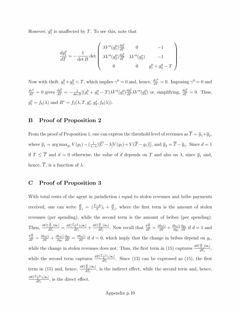
However, g01 is unaffected by T . To see this, note that

dg01dT

= − 1

detBdet

λV ′′(g01)

dg01dT

0 −1

λV ′′(g02)dg02dT

λV ′′(g∗2) −1

0 0 g01 + g02 − T

.

Now with theft, g01 +g02 < T , which implies γ0 = 0 and, hence, dγ0

dT= 0. Imposing γ0 = 0 and

dγ0

dT= 0 gives

dg01dT

= − 1detB

[(g01 + g02 − T )λV ′′(g01)dg01dTλV ′′(g02) or, simplifying,

dg01dT

= 0. Thus,

g01 = f6(λ) and R∗ = f5(λ, T, g∗1, g∗2, f6(λ)).

B Proof of Proposition 2

From the proof of Proposition 1, one can express the threshold level of revenues as T = g1+g2,

where g1 = arg maxg1 V (g1)− ( 11−λ)[U −λ[V (g1) +V (T − g1)]], and g2 = T − g1. Since d = 1

if T ≤ T and d = 0 otherwise, the value of d depends on T and also on λ, since g1 and,

hence, T , is a function of λ.

C Proof of Proposition 3

With total rents of the agent in jurisdiction i equal to stolen revenues and bribe payments

received, one can write RS i

= (T−SS

)i + BS i

, where the first term is the amount of stolen

revenues (per spending), while the second term is the amount of bribes (per spending).

Then,dE[(R

S i)|xi]

dTi=

dE[T−SS

)i|xi]dTi

+dE[B

S i)|xi]

dTi. Now recall that

dRS

dT= ∂h3()

∂T+ ∂h3()

∂g1

∂g1∂T

if d = 1 and

dRS

dT= ∂h4()

∂T+ ∂h4()

∂g1

∂g1∂T

= ∂h4()∂T

if d = 0, which imply that the change in bribes depend on g1,

while the change in stolen revenues does not. Thus, the first term in (15) capturesdE[B

S i)|xi]

dTi,

while the second term capturesdE[T−S

S)i|xi]

dTi. Since (13) can be expressed as (15), the first

term in (15) and, hence,dE[B

S i)|xi]

dTi, is the indirect effect, while the second term and, hence,

dE[T−SS

)i|xi]dTi

, is the direct effect.

Appendix p.10

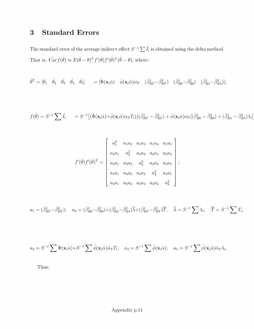
3 Standard Errors

The standard error of the average indirect effect S−1∑Ii is obtained using the delta method.

That is, ˆV arf(θ) ≈ E(θ − θ)Tf ′(θ)f ′(θ)T (θ − θ), where:

θT = [θ1 θ2 θ3 θ4 θ5] = [Φ(xiα) φ(xiα)αT (β1RT−β2

RT ) (β1R0−β2

R0) (β1Rλ−β2

Rλ)];

f(θ) = S−1∑

Ii = S−1[(Φ(xiα)+φ(xiα)αTTi))(β

1RT − β2

RT ) + φ(xiα)αT [(β1R0 − β2

R0) + (β1Rλ − β2

Rλ)λi]];

f ′(θ)f ′(θ)T =

a21 a1a2 a1a3 a1a4 a1a5

a2a1 a22 a2a3 a2a4 a2a5

a3a1 a3a2 a23 a3a4 a3a5

a4a1 a4a2 a4a3 a24 a4a5

a5a1 a5a2 a5a3 a5a4 a25

;

a1 = (β1RT−β2

RT ); a2 = (β1R0−β2

R0)+(β1Rλ−β2

Rλ)λ+(β1RT−β2

RT )T , λ = S−1∑

λi, T = S−1∑

Ti;

a3 = S−1∑

Φ(xiα)+S−1∑

φ(xiα)αTTi; a4 = S−1∑

φ(xiα); a5 = S−1∑

φ(xiα)αTλi.

Thus:

Appendix p.11

ˆV ar(S−1∑

Ii) ≈ σ21a

21 + 2σ12a1a2 + 2σ13a1a3 + 2σ14a1a4 + 2σ15a1a5

+σ22a

22 + 2σ23a2a3 + 2σ24a2a4 + 2σ25a2a5

+σ23a

23 + 2σ34a3a4 + 2σ35a3a5

+σ24a

24 + 2σ45a4a5

+σ25a

25,

where σ21, σ

22, ...σ

25 respectively denote ˆV ar(θ1), ˆV ar(θ2), ... ˆV ar(θ5), while σ12, σ13, ...σ45 re-

spectively denote ˆCov(θ1θ2), ˆCov(θ1θ3), . . . ˆCov(θ4θ5), and the standard error of the esti-

mated average indirect effect is simply

√ˆV ar(S−1

∑Ii). The standard error of the estimated

average total effect S−1∑Wi = D + S−1

∑Ii is

√ˆV ar(S−1

∑Wi) =

√ˆV ar(D) + ˆV ar(S−1

∑Ii) + 2 ˆCov(D, S−1

∑Ii).

4 The Sample

Recall that out of 1,620 municipalities for which fiscal data are available, 606 municipalities

comprise the ‘treatment’ group, where the (binary) treatment is the possibility of accumu-

lating wealth between 2011 and 2014 or, equivalently, of having the mayor re-elected in

2013, or of not experiencing a turnover. (Given that the possibility exists, one could then

estimate the continuous effect of government revenues on the mayor’s accumulated wealth,

using the structural model I propose.) The remaining 1,014 ‘untreated’ municipalities can

then be used to construct a placebo sample. These municipalities were not ‘treated’ in the

sense that there is no wealth accumulation possible. The assets declared in 2011 are different

from those declared in 2014 since they are from different mayors. One could compute the

difference in the value of these assets, but this would not capture wealth accumulation.

Appendix p.12

Thus, by estimating the structural model using the 606 municipalities, one would actually

draw inference about re-elected mayors, and be able to check the validity of the results by

comparing them with the results from estimating the model using the placebo sample.

The problem is that I do not have complete SALN data for all the 606 municipalities,

because not all of their mayors submitted in 2011 and 2014. Thus, I only have a selected

sample based on whether or not the municipality fully complied with the SALN requirements,

i.e. submitted in both years. Only 231 out of the 606 municipalities complied fully—this

implies an attrition rate of about 62%. The placebo sample is similarly constructed. Out of

the 1,014 untreated municipalities, only 166 had both their 2011 and 2014 mayors submit the

SALN and, thus, for which the difference between 2014 and 2011 assets can be computed.

Attrition among the untreated municipalities is thus higher at 84%. Included in those that

attrited from the main sample and the placebo sample are the 17 municipalities/cities from

the National Capital Region (NCR) in Luzon—more commonly known as Metro Manila,

thirteen of which did not experience a turnover in 2013. While it appears that fifteen of these

municipalities had their mayor submit the SALN in both 2011 and 2014 and could thus have

been included either in the main sample or the placebo sample, I have decided to exclude

the entire NCR since it is a clear outlier.23 Metro Manila is the most densely populated,

urbanized, and developed region in the country. Local administration in this region is also

different—the municipalities/cities are not aggregated into provinces, but are divided into

districts for statistical purposes. (These districts have no elected officials, nor receive the

IRA). Lastly, the SALNs of the mayors in Metro Manila are kept by the central office of the

Ombudsman, and not the Office of the Deputy Ombudsman for Luzon, which introduces

extra variation in the efficiency by which SALN records are stored and reproduced. As it

23In Appendix ??, I verify the robustness of results by re-estimating the model using a sample that includesthe NCR.

Appendix p.13

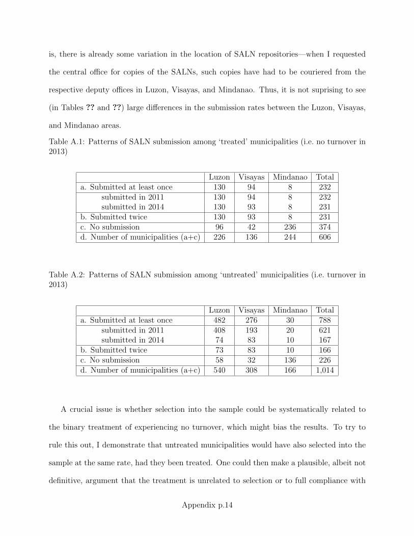
is, there is already some variation in the location of SALN repositories—when I requested

the central office for copies of the SALNs, such copies have had to be couriered from the

respective deputy offices in Luzon, Visayas, and Mindanao. Thus, it is not suprising to see

(in Tables ?? and ??) large differences in the submission rates between the Luzon, Visayas,

and Mindanao areas.

Table A.1: Patterns of SALN submission among ‘treated’ municipalities (i.e. no turnover in2013)

Luzon Visayas Mindanao Totala. Submitted at least once 130 94 8 232

submitted in 2011 130 94 8 232submitted in 2014 130 93 8 231

b. Submitted twice 130 93 8 231c. No submission 96 42 236 374d. Number of municipalities (a+c) 226 136 244 606

Table A.2: Patterns of SALN submission among ‘untreated’ municipalities (i.e. turnover in2013)

Luzon Visayas Mindanao Totala. Submitted at least once 482 276 30 788

submitted in 2011 408 193 20 621submitted in 2014 74 83 10 167

b. Submitted twice 73 83 10 166c. No submission 58 32 136 226d. Number of municipalities (a+c) 540 308 166 1,014

A crucial issue is whether selection into the sample could be systematically related to

the binary treatment of experiencing no turnover, which might bias the results. To try to

rule this out, I demonstrate that untreated municipalities would have also selected into the

sample at the same rate, had they been treated. One could then make a plausible, albeit not

definitive, argument that the treatment is unrelated to selection or to full compliance with

Appendix p.14

the SALN requirement.24

Now, the rate of full compliance among the treated is 232606∗ 231

232= 38%. (As shown in Table

??, there are 606 municipalities that did not experience a turnover and were thus treated;

among these, 232 submitted a SALN at least once—232 in 2011 and 231 in 2014, and among

these 232 municipalities, 231 submitted twice. Thus, the probability of submitting the SALN

once is 232606

; and the probability of submitting a second time is 231232

, and their joint probability

is the rate of full compliance.)

From Table ??, there are 788 untreated municipalities whose 2011 and/or 2014 mayor

submitted her SALN. To demonstrate that untreated municipalities, had they been treated,

would have been selected into the (main) sample at the same rate that a treated municipality

is selected, one would need to show how a mayor in these 788 municipalities would behave,

that is, whether she would submit the SALN and, conditional on having submitted, whether

she would submit a second time if she were re-elected. Now, there are actually two types of

mayors in these municipalities—a 2011 mayor, and a 2014 mayor. (Although an untreated

municipality can have two SALN submissions, i.e. one from its 2011, and another from its

2014, mayor, a particular mayor in an untreated municipality can only submit once). The

rate of one/first-time submission of the 2011-mayor type is 6211,014

= 61%. Assuming this type

of mayor would submit a second time at the same rate as a mayor in a treated municipality

would, i.e. at 231232

= 99.6%, then the rate of full compliance of this type of mayor would

be the joint probability 61 ∗ 99.6% = 60.76%.25 Analogously, the rate of one/first-time

submission for a 2014 mayor is 1671,014

= 16.5%—with a 99.6% resubmission rate, their rate

24What is ultimately of interest is the continuous treatment of revenues (although necessary for this isreceipt of the binary treatment of not experiencing a turnover). Thus, in Appendix ??, I show that selectioneither into the main or the placebo sample is unrelated to revenues by demonstrating that in both thesesamples, submitting the SALN twice is not significantly associated with the municipality’s ira.

25In fact, Table ?? implies that conditional on having submitted in 2014, an untreated municipality wouldhave almost certainly submitted in 2011, i.e. at the rate 166

167 = 99.4%. This, however, does not pertain to themayor’s behavior—the 167 mayors that submitted in 2014 could not have been the same 166 mayors thatsubmitted in 2011.

Appendix p.15

of full compliance would be 16.5 ∗ 99.6% = 16.43%. Taking the simple average gives the

hypothetical rate of full compliance of untreated municipalities: 60.76+16.432

= 38.6%, which

is very close to the 38% compliance rate of the treated municipalities.

In taking the simple, rather than some weighted, average, one implicitly assumes that

the 2011 and 2014 mayors in the untreated municipalities are the same in all others respects

(except in their one/first-time SALN submission rate). Thus, it is as though there are only

1,014 mayors among the untreated municipalities between 2011 and 2014, although in fact

there are 1, 014 ∗ 2 = 2, 028. Viewing the 2011 and 2014 mayors of a municipality as though

they were only one mayor arguably makes the untreated municipalities more comparable to

the treated municipalities, since the latter have only one mayor each.

As for the difference in the one/first-time submission rates between the 2011 and 2014

mayors in untreated municipalities, the relatively higher rate for the 2011 mayors is suggestive

of lags or delays in the submission. That is, the 2011 mayors may simply have had more

time to turn in their SALN than the 2014 mayors who have just started their first year

of office. This could explain why mayors in the treated municipalities have a high rate

(99%) of second-time submission—by 2014, they already have an existing SALN which they

could easily modify or re-submit as is. The issue remains, however, as to why the 2011

submission rate is lower for the treated than the untreated municipalities, i.e. 232606

= 38.28%

vs. 6211,014

= 61%.

First note that this difference is largely driven by Mindanao and, to a smaller extent, by

Luzon. Tables ?? and ?? imply that in Visayas, the 2011 submission rates in the treated

and the untreated municipalities are similar at 93136

= 68% and 193308

= 63%, respectively. The

largest difference in the 2011 submission rates between treated and untreated municipali-

ties appears to have come from Mindanao. Among the untreated, the rate is 20166

= 12%,

while among the treated, it is 8244

= 0.03%, which implies a difference of 12−0.030.03

= 399%.

Appendix p.16

Meanwhile, the difference in Luzon is only 31%, that is, 408540

= 76% among the untreated

vs. 130226

= 58% among the treated. Also, recall that the Luzon municipalities excludes the

17 from Metro Manila, most of which would have been considered treated. Including them

would have raised the 2011 submission rate of treated municipalities in Luzon to about 60%,

which would be closer to the rate among the untreated.26

Two facts about Mindanao are noteworthy. One is that it is the poorest and least

developed area in the country, burdened by ongoing insurgency and armed conflict with

Muslim separatist groups. The other is that local politics is far less competitive—note that

244244+166

= 60% of municipalities in Mindanao experienced no turnover in 2013, compared to

226226+540

= 35% and 136136+308

= 31% in Luzon and Visayas, respectively.27 One could envisage

that both of these factors contribute to low SALN submission rates, as administrative capac-

ity may be lower, and record-keeping less reliable, in Mindanao. Note, then, that compared

to Luzon and Visayas, the rates of submission in 2011, and in 2014, and of submitting twice,

are all lower (while the rate of non-submission is higher), whether among the treated or the

untreated municipalities. That the difference in 2011 submission rates between Mindanao

and Luzon-Visayas is more pronounced among the treated municipalities further makes plau-

sible that administrative capacity and record-keeping may be more lax when there is weak

political competition such that there is no turnover, and even more so in less developed areas

(i.e. Mindanao).

Ultimately, however, what determines selection into the (main) sample is whether or

not the mayors in treated municipalities submitted the SALN in both years. Similarly, the

placebo sample consists of untreated municipalities whose 2011 mayor and 2014 mayor both

26Thirteen of the seventeen Metro Manila mayors were reelected, and for all of them the 2011 SALNare available. This implies that the 2011 submission rate among the treated in Luzon would have been130+13226+13 = 60%. Four were not reelected, all of whom provided 2011 SALNs. This implies that the Luzon

2011 submission rate among the untreated would have been 408+4540+4 = 76%. This gives a difference of 27%.

27Elections in Mindanao are also fraught with allegations of fraud and incidence of violence. See, e.g.http://newsinfo.inquirer.net/792073/violence-vote-buying-still-rampant-in-ph-polls-us-ngo.

Appendix p.17

submitted. Recall that the rate of inclusion into the placebo sample ( 1661,014

= 16%) is actually

much lower than the rate of selection into the main sample (231606

= 38%). One possibility is

that while lower political competition (that enables re-election in the municipality) could be

associated with lower administrative and record-keeping capacities, the mayors themselves,

once re-elected, might be more efficient and conscientious in submitting the SALN (on time).

This might explain why, conditional on having submitted in 2011, a re-elected mayor almost

certainly submits again in 2014 (i.e. at rate 99.6%), whereas a mayor that is elected for the

first time in 2013 is far less likely to have submitted a SALN in 2014 (i.e. at rate 16.5%).

If the latter were re-elected in the next election (2016), it could very well be that she will

submit again (i.e. at rate 99.6%). This, then, provides an alternative justification for the

earlier calculation that 38.6% of untreated municipalities would have been selected into the

sample had they not experienced a turnover.

The foregoing analysis suggests that the selection of a municipality into the sample is

exogenous to the mayor’s rent-seeking behavior. That a mayor has on (retrievable) record

a 2011 and a 2014 SALN might more plausibly have to do with the ability of the mayor’s

office to ensure that, each year, the mayor receives the SALN form, fills it in, and is sent

to the appropriate (deputy) Ombudsman’s office on time, as well as the ability of the latter

to maintain SALN records and provide complete copies to whoever might request them.

Given that the penalties for failure to submit the SALN are non-trivial, it would be rational

for a mayor to submit the SALN at least once, or at random years, during her term/s of

office. (Recall that the SALN is required for every year in office.) For a rent-seeking mayor to

deliberately fail to submit in the specific years 2011 and 2014 in order to conceal accumulated

rents implies that she anticipates that someone would take copies of her 2011 and 2014 SALNs

and be able to infer that the difference in the value of the assets reported therein is too high

to be legitimate. To my best knowledge, the Office of the Ombudsman does not routinely

Appendix p.18

make this kind of calculation. In fact, newspapers and journalists periodically publish the

net worth of public officials, especially during elections, but no one has been prosecuted for

having reported too large a net worth. On the contrary, what usually invites further scrutiny

are allegations of unreported assets or failure to submit the SALN.

Note, then, that the claim that the particular sample used in this paper is random does

not ignore the possibility that rent-seeking mayors are wary of faithfully submitting the

SALNs, lest they reveal ill-gotten wealth. It could very well be that they deliberately fail

to submit in some years and/or omit to report some assets in the SALN.28 Rather, the

argument is that given the costs of violating SALN requirements, even a rent-seeking mayor

would want to submit an accurate SALN at least once. That she would deliberately exclude

the specific years 2011 and 2014 is what is untenable, which makes the particular sample

random.

5 Descriptive Statistics

Appendix ?? presents summary statistics of the proxy variables in multiple tables. The first

table, Table ??, uses all 1,620 municipalities. Table ?? uses only the 606 municipalities that

were ’treated’ with re-election or no turnover—the intended sample, while Table ?? uses the

231 municipalities from this subset whose mayor submitted the SALN in 2011 and 2014—the

selected sample. Table ?? uses the 1,014 ‘untreated’ municipalities that had a turnover and

thus had two mayors in the sample period, while Table ?? uses the 166 municipalities from

this subset whose two mayors each submitted a SALN—the placebo sample.

What is most noteworthy is the difference in asset accumulation between the treated

and untreated municipalities. Table ?? shows that between 2011 and 2014, on average, a

28The high attrition rates in both the main and placebo samples are thus unsurprising. Also, as shown inAppendix ??, incidences of misreporting in some components of the mayor’s net worth are also apparent inthe sample.

Appendix p.19

re-elected mayor accumulated (net) assets equivalent to 0.054 of total government spending

in her municipality (i.e. mean networth = 0.054). In contrast, mean networth for mu-

nicipalities that had a turnover is −0.044 (Table ??). This confirms that in the placebo

sample, no wealth accumulation is possible. Indeed, networth in this sample only captures

the difference in net worth between the 2011 and the 2014 mayor.

It also appears that, with the exception of the asset variables, the main sample and

the placebo sample are similar—for most of the proxy variables, the mean values in Table

?? are close to those in Table ??. However, mean ira seems lower in municipalities that

had no turnover than those that had (Tables ?? and ??). Also, while the mean ira among

municipalities with no turnover is 90 (million pesos—see Table ??), the subset selected

into the main sample has higher mean ira at 98.5 (Table ??). On the other hand, while

mean ira among municipalities that experienced a turnover is 105 (see Table ??), the subset

selected into the placebo sample has mean ira equal to 120 (Table ??). Since ira is actually

the (continuous) treatment of interest in the model, one would be rightly concerned if this

treatment were to determine sample selection. I thus try to demonstrate that this is unlikely.

First note that since the model is only concerned with measuring the effect of ira on

rent accumulation, the relevant sample of interest consists only of those 606 municipalities

whose mayor was re-elected in 2013 and, hence, had the opportunity to earn rents between

2011-2014. Thus, necessary for a municipality to be treated with ‘rent-generating’ ira is

having been ‘treated’ with re-election. Table ?? shows that the latter binary treatment

appears to be exogenous in the sense that it is unrelated to all the proxy variables in the

model. However, sufficiency requires that ira itself is exogenous to sample selection. Thus,

Table ?? tests which variables possibly determine whether or not the municipality submits

the SALN in 2011 and in 2014. It appears that with the exception of electricity, none of the

variables capturing municipality characteristics determine whether two different mayors from

Appendix p.20

the same municipality would both submit their SALN. This suggests that the placebo sample

of 166 municipalities is a random subset of the 1,014 municipalities that had a turnover. In

contrast, some of the variables seem to affect whether or not the same re-elected mayor would

submit twice. In particular, selection into the main sample appears to be negatively related

with some spending variables (construction, pubserv, health, econ), negatively related to

electricity, and positively or negatively related to some proxies for λ. Note, however, that

when controlling for these variables, ira itself is insignificant.

Appendix p.21

Table A.3: Determinants of no turnover in 2013

VARIABLES No TurnoverChange in Net Worth per Spending 0.0605

(0.0574)Change in Real Assets per Spending 0.0260

(0.261)Change in Personal Assets per Spending -0.0243

(0.0821)Change in Liabilities per Spending -0.207

(0.221)Construction Spending -0.00169

(0.00635)Capital and Investment Spending 0.895

(1.236)Public Services Spending 0.153

(1.031)Education Spending -0.362

(2.087)Health Spending -0.768

(1.520)Labor Spending 7.005

(6.706)Housing Spending 0.876

(1.401)Social Welfare Spending 0.276

(1.323)Economic Services Spending 0.124

(1.094)No Debt 0.0262

(0.0797)Proportion of Population Aged 15-24 1.312

(2.711)Proportion of School-Age Youth Enrolled in School -0.845

(1.386)Proportion of Population Who Are Employed 0.290

(0.767)

Appendix p.22

Proportion of Population in Professional Jobs -1.257(1.047)

Proportion of Households That Have Electricity -0.00417(0.352)

Proportion of Households That Have At Least One Cellphone -0.0306(0.491)

Proportion of Population Who are Registered Voters 0.101(0.429)

Internal Revenue Allotment 0.00106(0.00215)

Proportion of Households Who Own the Land They Occupy -0.307(0.281)

Proportion of Households Who Own the House They Occupy 0.233(0.492)

Income Classification 1-6, with 6 as Highest Level 0.00961(0.0460)

Urban Municipality -0.0499(0.155)

Log of the Land Area of the Municipality -0.0410(0.0676)

Log of the Average Population Between 2010-2015 -0.00627(0.0875)

Observations 278R-squared 0.066

Standard errors in parentheses*** p<0.01, ** p<0.05, * p<0.1

Appendix p.23

Table A.4: Determinants of submitting the SALN in both years, for municipalities that hadno turnover in 2013 vs. those that had

(1) (2) (3) (4)Submitted in 2011 and 2014 Submitted in 2011 and 2014

VARIABLES No Turnover With Turnover

Construction Spending 0.000890 6.41e-05(0.00520) (0.00197)

Capital and Investment Spending -1.437 -0.349(0.879) (0.498)

Public Services Spending -1.459* -0.182(0.748) (0.453)

Education Spending -0.576 0.103(1.459) (0.783)

Health Spending -2.541** -0.0562(0.995) (0.578)

Labor Spending 2.075 -3.888(4.857) (4.463)

Housing Spending 0.600 -0.575(1.149) (0.602)

Social Welfare Spending -0.734 -0.272(0.976) (0.563)

Economic Services Spending -1.655** -0.170(0.777) (0.459)

No Debt -0.0180 -0.0253(0.0520) (0.0311)

Proportion of Population Aged 15-24 5.530*** 0.972(1.671) (0.996)

Proportion of School-Age Youth Enrolled in School -1.943** -0.213(0.808) (0.500)

Proportion of Population Who Are Employed 0.303 0.208(0.417) (0.276)

Proportion of Population in Professional Jobs -0.0207 0.416(0.668) (0.328)

Proportion of Households That Have Electricity -0.493*** -0.263**(0.173) (0.106)

Appendix p.24

Proportion of Households That Have At Least One Cellphone 1.021*** 0.172(0.239) (0.152)

Proportion of Population Who are Registered Voters -0.269 0.150(0.240) (0.155)

Internal Revenue Allotment 0.00239 -0.000559(0.00179) (0.000797)

Proportion of Households Who Own the Land They Occupy 0.0144 0.151(0.168) (0.0975)

Proportion of Households Who Own the House They Occupy -0.127 -0.341(0.307) (0.210)

Income Classification 1-6, with 6 as Highest Level -0.00625 -0.0189(0.0326) (0.0181)

Urban Municipality -0.0131 -0.0584(0.129) (0.0554)

Log of the Land Area of the Municipality 0.0171 -0.0131(0.0425) (0.0236)

Log of the Average Population Between 2010-2015 -0.0796 0.0166(0.0631) (0.0345)

Average Net Worth per Spending 0.0135 -0.0119(0.0470) (0.0207)

Average Real Assets per Spending -0.00714 -0.212**(0.0251) (0.105)

Average Personal Assets per Spending -0.0113 0.135*(0.0544) (0.0745)

Average Liabilities per Spending 0.0509 0.439**(0.108) (0.181)

Constant 1.719 0.994*** 0.360 0.207***(1.212) (0.00534) (0.766) (0.0166)

Observations 512 232 820 788R-squared 0.156 0.002 0.034 0.012

Standard errors in parentheses*** p<0.01, ** p<0.05, * p<0.1

Appendix p.25

6 Summary Statistics

Table A.5: Summary Statistics for all 1,620 municipalities

(1) (2) (3) (4) (5)VARIABLES N mean sd min max

Total Spending 1,620 153.5 471.5 16.70 9,103Change in Net Worth per Spending 397 0.0129 0.693 -9.187 9.012Change in Real Assets per Spending 397 0.00996 0.193 -1.548 2.670Change in Personal Assets per Spending 397 -0.000543 0.474 -8.884 2.213Change in Liabilities per Spending 397 0.0170 0.208 -0.318 3.816Construction Spending 1,620 18.86 104.6 0 2,998Capital and Investment Spending 1,620 0.0826 0.0858 0 0.612Public Services Spending 1,620 0.582 0.123 0.180 0.963Education Spending 1,620 0.0182 0.0249 0 0.285Health Spending 1,620 0.0770 0.0316 0 0.236Labor Spending 1,620 0.000426 0.00333 0 0.0625Housing Spending 1,620 0.0104 0.0279 0 0.384Social Welfare Spending 1,620 0.0518 0.0337 0 0.356Economic Services Spending 1,620 0.148 0.0771 0.0141 0.640No Debt 1,620 0.393 0.489 0 1Proportion of Population Aged 15-24 1,474 0.193 0.0129 0.0745 0.247Proportion of School-Age Youth Enrolled in School 1,474 0.274 0.0274 0.0248 0.401Proportion of Population Who Are Employed 1,474 0.334 0.0562 0.156 0.857Proportion of Population in Professional Jobs 1,474 0.107 0.0489 0.00376 0.425Proportion of Households That Have Electricity 1,474 0.762 0.193 0 0.997Proportion of Households That Have At Least One Cellphone 1,474 0.645 0.151 0.110 1Proportion of Population Who are Registered Voters 1,460 0.593 0.113 0.243 2.419Internal Revenue Allotment 1,620 99.28 163.4 16.58 2,787Proportion of Households Who Own the Land They Occupy 1,474 0.391 0.184 0.0152 0.994Proportion of Households Who Own the House They Occupy 1,474 0.853 0.0754 0.0645 1Income Classification 1-6, with 6 as Highest Level 1,447 3.115 1.468 1 6Urban Municipality 1,460 0.0562 0.230 0 1Log of the Land Area of the Municipality 1,460 9.526 0.912 6.148 12.30Log of the Average Population Between 2010-2015 1,460 10.30 0.762 5.313 12.69Average Net Worth per Spending 1,020 0.160 0.676 -0.0802 19.22Average Real Assets per Spending 1,020 0.0903 0.319 0 8.840Average Personal Assets per Spending 1,020 0.0745 0.208 0 4.480Average Liabilities per Spending 1,020 0.0305 0.0832 0 1.912Percentage Growth of Net Worth 229 27,535 260,784 -196.2 2.842e+06Percentage Growth of Real Assets 210 436.4 5,681 -193.5 82,328Percentage Growth of Personal Assets 214 190.3 1,027 -100 12,422Percentage Growth of Liabilities 187 242.6 1,202 -168.6 13,233

Appendix p.26

Table A.6: Summary Statistics for the Intended Sample, i.e. the 606 municipalities that hadno turnover

(1) (2) (3) (4) (5)VARIABLES N mean sd min max

Total Spending 606 152.6 549.8 20.94 9,103Change in Net Worth per Spending 231 0.0540 0.641 -2.960 9.012Change in Real Assets per Spending 231 0.000949 0.127 -1.548 0.584Change in Personal Assets per Spending 231 0.0123 0.103 -1.009 0.728Change in Liabilities per Spending 231 0.00462 0.0467 -0.318 0.246Construction Spending 606 18.50 106.5 0 2,362Capital and Investment Spending 606 0.0801 0.0798 0 0.565Public Services Spending 606 0.592 0.122 0.248 0.963Education Spending 606 0.0174 0.0242 0 0.184Health Spending 606 0.0777 0.0325 0 0.206Labor Spending 606 0.000505 0.00409 0 0.0625Housing Spending 606 0.00953 0.0253 0 0.254Social Welfare Spending 606 0.0499 0.0308 0 0.302Economic Services Spending 606 0.145 0.0802 0.0141 0.640No Debt 606 0.404 0.491 0 1Proportion of Population Aged 15-24 552 0.193 0.0139 0.0745 0.238Proportion of School-Age Youth Enrolled in School 552 0.276 0.0299 0.0248 0.401Proportion of Population Who Are Employed 552 0.333 0.0597 0.200 0.857Proportion of Population in Professional Jobs 552 0.102 0.0431 0.0167 0.327Proportion of Households That Have Electricity 552 0.747 0.194 0 0.997Proportion of Households That Have At Least One Cellphone 552 0.625 0.154 0.145 1Proportion of Population Who are Registered Voters 553 0.598 0.105 0.243 1.468Internal Revenue Allotment 606 89.67 152.7 16.58 2,787Proportion of Households Who Own the Land They Occupy 552 0.395 0.187 0.0152 0.992Proportion of Households Who Own the House They Occupy 552 0.856 0.0851 0.0645 0.996Income Classification 1-6, with 6 as Highest Level 550 3.304 1.467 1 6Urban Municipality 553 0.0325 0.178 0 1Log of the Land Area of the Municipality 553 9.440 0.864 6.548 11.89Log of the Average Population Between 2010-2015 553 10.23 0.758 5.313 12.34Average Net Worth per Spending 232 0.156 0.415 -0.00302 4.583Average Real Assets per Spending 232 0.116 0.596 0 8.840Average Personal Assets per Spending 232 0.0801 0.204 0 2.237Average Liabilities per Spending 232 0.0280 0.0456 0 0.364Percentage Growth of Net Worth 229 27,535 260,784 -196.2 2.842e+06Percentage Growth of Real Assets 210 436.4 5,681 -193.5 82,328Percentage Growth of Personal Assets 214 190.3 1,027 -100 12,422Percentage Growth of Liabilities 187 242.6 1,202 -168.6 13,233

Appendix p.27

Table A.7: Summary Statistics for the Selected Sample, i.e. the 231 municipalities whosemayor submitted the SALN in 2011 and 2014

(1) (2) (3) (4) (5)VARIABLES N mean sd min max

Total Spending 231 145.7 313.5 22.16 3,820Change in Net Worth per Spending 231 0.0540 0.641 -2.960 9.012Change in Real Assets per Spending 231 0.000949 0.127 -1.548 0.584Change in Personal Assets per Spending 231 0.0123 0.103 -1.009 0.728Change in Liabilities per Spending 231 0.00462 0.0467 -0.318 0.246Construction Spending 231 17.32 44.16 0 424.6Capital and Investment Spending 231 0.0882 0.0913 0 0.565Public Services Spending 231 0.578 0.134 0.248 0.963Education Spending 231 0.0190 0.0250 0 0.163Health Spending 231 0.0726 0.0318 0 0.162Labor Spending 231 0.000808 0.00570 0 0.0625Housing Spending 231 0.0122 0.0318 0 0.254Social Welfare Spending 231 0.0489 0.0369 0 0.302Economic Services Spending 231 0.146 0.0821 0.0160 0.640No Debt 231 0.338 0.474 0 1Proportion of Population Aged 15-24 198 0.195 0.0148 0.0745 0.234Proportion of School-Age Youth Enrolled in School 198 0.270 0.0305 0.0248 0.370Proportion of Population Who Are Employed 198 0.342 0.0647 0.243 0.857Proportion of Population in Professional Jobs 198 0.109 0.0516 0.0289 0.327Proportion of Households That Have Electricity 198 0.754 0.201 0.207 0.985Proportion of Households That Have At Least One Cellphone 198 0.662 0.156 0.210 1Proportion of Population Who are Registered Voters 205 0.591 0.107 0.243 1.347Internal Revenue Allotment 231 98.52 119.8 24.29 1,084Proportion of Households Who Own the Land They Occupy 198 0.389 0.181 0.0962 0.941Proportion of Households Who Own the House They Occupy 198 0.842 0.0936 0.0645 0.970Income Classification 1-6, with 6 as Highest Level 204 3 1.525 1 6Urban Municipality 205 0.0488 0.216 0 1Log of the Land Area of the Municipality 205 9.553 0.890 7.296 11.89Log of the Average Population Between 2010-2015 205 10.34 0.804 5.313 12.34Average Net Worth per Spending 231 0.156 0.416 -0.00302 4.583Average Real Assets per Spending 231 0.116 0.598 0 8.840Average Personal Assets per Spending 231 0.0804 0.205 0 2.237Average Liabilities per Spending 231 0.0281 0.0456 0 0.364Percentage Growth of Net Worth 229 27,535 260,784 -196.2 2.842e+06Percentage Growth of Real Assets 210 436.4 5,681 -193.5 82,328Percentage Growth of Personal Assets 214 190.3 1,027 -100 12,422Percentage Growth of Liabilities 187 242.6 1,202 -168.6 13,233

Appendix p.28

Table A.8: Summary Statistics for the 1,014 Municipalities that had a Turnover

(1) (2) (3) (4) (5)VARIABLES N mean sd min max

Total Spending 1,014 154.1 418.0 16.70 7,057Change in Net Worth per Spending 166 -0.0442 0.758 -9.187 1.295Change in Real Assets per Spending 166 0.0225 0.258 -0.329 2.670Change in Personal Assets per Spending 166 -0.0185 0.725 -8.884 2.213Change in Liabilities per Spending 166 0.0343 0.317 -0.284 3.816Construction Spending 1,014 19.07 103.5 0 2,998Capital and Investment Spending 1,014 0.0840 0.0892 0 0.612Public Services Spending 1,014 0.577 0.122 0.180 0.903Education Spending 1,014 0.0186 0.0254 0 0.285Health Spending 1,014 0.0766 0.0310 0 0.236Labor Spending 1,014 0.000379 0.00277 0 0.0373Housing Spending 1,014 0.0109 0.0293 0 0.384Social Welfare Spending 1,014 0.0529 0.0352 0 0.356Economic Services Spending 1,014 0.149 0.0751 0.0187 0.637No Debt 1,014 0.387 0.487 0 1Proportion of Population Aged 15-24 922 0.193 0.0123 0.127 0.247Proportion of School-Age Youth Enrolled in School 922 0.273 0.0259 0.182 0.371Proportion of Population Who Are Employed 922 0.334 0.0540 0.156 0.630Proportion of Population in Professional Jobs 922 0.110 0.0518 0.00376 0.425Proportion of Households That Have Electricity 922 0.771 0.193 0.0210 0.993Proportion of Households That Have At Least One Cellphone 922 0.656 0.148 0.110 0.947Proportion of Population Who are Registered Voters 907 0.590 0.118 0.271 2.419Internal Revenue Allotment 1,014 105.0 169.3 17.08 2,624Proportion of Households Who Own the Land They Occupy 922 0.389 0.183 0.0501 0.994Proportion of Households Who Own the House They Occupy 922 0.852 0.0689 0.560 1Income Classification 1-6, with 6 as Highest Level 897 2.999 1.457 1 6Urban Municipality 907 0.0706 0.256 0 1Log of the Land Area of the Municipality 907 9.578 0.937 6.148 12.30Log of the Average Population Between 2010-2015 907 10.35 0.760 7.146 12.69Average Net Worth per Spending 788 0.161 0.736 -0.0802 19.22Average Real Assets per Spending 788 0.0827 0.165 0 1.719Average Personal Assets per Spending 788 0.0729 0.210 0 4.480Average Liabilities per Spending 788 0.0313 0.0914 0 1.912

Appendix p.29

Table A.9: Summary Statistics for the Placebo Sample, i.e. the 166 municipalities that hada turnover and whose two mayors submitted a SALN

(1) (2) (3) (4) (5)VARIABLES N mean sd min max

Total Spending 166 158.4 249.8 22.52 1,827Change in Net Worth per Spending 166 -0.0442 0.758 -9.187 1.295Change in Real Assets per Spending 166 0.0225 0.258 -0.329 2.670Change in Personal Assets per Spending 166 -0.0185 0.725 -8.884 2.213Change in Liabilities per Spending 166 0.0343 0.317 -0.284 3.816Construction Spending 166 16.60 34.70 0 268.1Capital and Investment Spending 166 0.0751 0.0727 0 0.419Public Services Spending 166 0.582 0.127 0.270 0.903Education Spending 166 0.0181 0.0224 0 0.104Health Spending 166 0.0704 0.0320 0 0.209Labor Spending 166 0.000278 0.00251 0 0.0317Housing Spending 166 0.00719 0.0230 0 0.161Social Welfare Spending 166 0.0518 0.0352 0 0.244Economic Services Spending 166 0.158 0.0766 0.0362 0.589No Debt 166 0.331 0.472 0 1Proportion of Population Aged 15-24 128 0.195 0.0119 0.163 0.236Proportion of School-Age Youth Enrolled in School 128 0.273 0.0216 0.227 0.331Proportion of Population Who Are Employed 128 0.343 0.0462 0.253 0.490Proportion of Population in Professional Jobs 128 0.113 0.0549 0.0400 0.291Proportion of Households That Have Electricity 128 0.740 0.208 0.0354 0.976Proportion of Households That Have At Least One Cellphone 128 0.652 0.138 0.360 0.894Proportion of Population Who are Registered Voters 138 0.606 0.182 0.336 2.419Internal Revenue Allotment 166 120.3 142.6 22.91 852.9Proportion of Households Who Own the Land They Occupy 128 0.395 0.204 0.0645 0.967Proportion of Households Who Own the House They Occupy 128 0.837 0.0638 0.638 0.990Income Classification 1-6, with 6 as Highest Level 134 2.933 1.415 1 6Urban Municipality 138 0.0580 0.235 0 1Log of the Land Area of the Municipality 138 9.709 0.889 7.524 11.90Log of the Average Population Between 2010-2015 138 10.36 0.685 7.775 11.83Average Net Worth per Spending 166 0.139 0.374 -0.000498 4.655Average Real Assets per Spending 166 0.0756 0.133 0 1.335Average Personal Assets per Spending 166 0.0930 0.360 0 4.480Average Liabilities per Spending 166 0.0426 0.157 0 1.912

7 Selection Model

In the following, I formally show that the estimates are unaffected in spite of the fact that

many jurisdictions/municipalities drop out of the sample because some politicians fail to

submit the SALNs for the two years 2011 and 2014. In particular, I first demonstrate

Appendix p.30

in subsection ?? that there is no selection bias if all other factors that affect government

spending and rents (apart from revenues and λ ) are independent of the politician’s decision

to submit the SALN, which I call “independence from selection”. Then, I show that there is

still no selection bias under weaker assumptions if the only variables affecting the politician’s

decision to submit are either λ and T , i.e. ”selection on explanatory variables”, or government

spending and rents, i.e “selection on outcome variables”. In subsection ??, I obtain analogous

results in the case when the politician’s decision to submit the SALN also depends on whether

or not the politician would accurately report the items on the SALN.

A

Jurisdiction j is selected into the sample if the politician from j submits her SALN for both

years 2011 and 2014 (from which the difference in the value of her assets can be computed).

Non-submission of the SALN for each year in office is a crime that is punishable by law. On

the other hand, submitting the SALN makes a corrupt politician vulnerable to allegations of

corruption, prosecution in court, and conviction. Thus, the politician, in deciding whether

or not to submit the SALN in 2011 and 2014, weighs the utility of avoiding sanctions for

failure to submit, against the (dis)utility from providing evidence/information on her assets

which may be used against her.

Thus, denote the net utility of the politician j from submitting the SALN for both years

2011 and 2014 as Sj, and suppose it is determined by:

Sj = vjαj + wj,

where vj are the factors that affect Sj, while wj is the error term. The politician submits

the SALN for both years and, hence, is selected into the sample, if net utility Sj is positive.

Appendix p.31

That is, letting sj indicate submission for both years/selection into the sample, sj = 1 if

Sj = vjαj + wj > 0 or wj > −vjα, and sj = 0 otherwise.

Recall that we are interested in estimating the system

yj = xjγj + uj.

However, since yj can only be observed if sj = 1, what we are actually only able to estimate

is:

E(yj|sj = 1,xj) = E(yj|wj > −vjα,xj).

Consider the following assumptions:

(a) wj ⊥ vj, wj ⊥ xj

(b) E(uj|xj) = E(uj) = 0

(c) uj ⊥ wj

(d) uj ⊥ vj

(e) xj ⊥ vj

Proposition 4. Independence from selection

If (a), (b), (c), (d), and (e) hold, then there is no selection bias.

Proof. Under (a) and (e), E(yj|sj = 1,xj) = xjγj + E(uj|wj > −vjα,xj) which, under (c)

and (d), is equal to xjγj + E(uj|xj). Under (b), this reduces to xjγj. �

Proposition 5. Selection on explanatory variables

Suppose vj = xj. If (a), (b), and (c) hold, then there is no selection bias.

Appendix p.32

Proof. With vj = xj, E(yj|sj = 1,xj) = E(yj|wj > −xjα,xj). Under (a) and (c), this is

equal to xjγj + E(uj|xj) which, under (b), reduces to xjγj.

�

Proposition 6. Selection on outcome variables

Suppose vj = yj. If (a) and (b) hold, then there is no selection bias.

Proof. With vj = yj, E(yj|sj = 1,xj) = E(vj|wj > −vjα,xj). Under (a), this is equal to

E(vj|xj) = E(yj|xj) = xjγj + E(uj|xj) which, under (b), reduces to xjγj.

�

B

Now suppose that the net utility from submitting both SALNs is affected by whether or

not the politician will falsify, or inaccurately report the required information on the SALN.

Specifically, let rj = 1 indicate accurate reporting, and 0 otherwise, and the net utility Sj is

now given by:

Sj = vjαj + δrj + wj.

Consider the following additional assumptions:

(i) rj ⊥ xj

(ii) rj ⊥ uj

(iii) rj ⊥ vj

Proposition 7. Independence from selection

If assumptions (a), (b), (c), (d), (e), (i), and (ii) hold, then there is no selection bias.

Appendix p.33

Proof. Under (a), (e), and (i), E(yj|sj = 1,xj) = xjγj + E(uj|wj > −vjα − δrj,xj) which,

under (c), (d), and (ii), is equal to xjγj + E(uj|xj). Under (b), this reduces to xjγj.

�

Proposition 8. Selection on explanatory variables

Suppose vj = xj. If (a), (b), (c), (i) and (ii) hold, then there is no selection bias.

Proof. With vj = xj, E(yj|sj = 1,xj) = E(yj|wj > −xjα− δrj,xj). Under (a), (c), (i), and

(ii), this is equal to xjγj + E(uj|xj) which, under (b), reduces to xjγj.

�

Proposition 9. Selection on outcome variables

Suppose vj = yj. If (a), (b), and (iii) hold, then there is no selection bias.

Proof. With vj = yj, E(yj|sj = 1,xj) = E(vj|wj > −vjα − δrj,xj). Under (a) and (iii),

this is equal to E(vj|xj) = E(yj|xj) = xjγj + E(uj|xj) which, under (b), reduces to xjγj.

�

8 Wealth Accumulation

The difference in the net worth of a mayor between the years 2011 and 2014 should be

close to zero, because any (legitimate) increase in salaries and allowances of the mayor

would be closely matched by an increase in her expenses. Nevertheless, even accounting for

the possibility that mayors are financially prudent, and that they may have other sources of

legitimate income, their asset performance and spending patterns are dependent on economic

conditions and, to that extent, are expected to be consistent with macroeconomic trends.

Overall, the Philippine economy grew by about 18% in the sample period—from a GDP

per capita of $ 2129.5 in 2010 to 2505.8 in 2014. Between 2010 to 2014, the annual GDP

Appendix p.34

growth rate reached a high of 9% and a low of about 2%.29 Minimum wages grew by about

20%, from a monthly minimum wage of 7,995 (Philippine pesos P ) in 2010, to 9,581.8 in

2014. The growth of GDP from Public Administration (which would include salaries in the

public sector) is more modest—in 2010 it reached a high of 72,000 (million P ), and in 2014,

82,000, implying a growth rate of about 14%. Meanwhile, spending likely outstripped the

wage growth of public servants, since consumer spending grew by 26%, from 950,000 (million

P ) in 2010 to 1,200,000 in 2014. Vehicle sales alone grew by 50%—4,000 (million P ) in 2010

to 6,000 in 2014. By these trends, it is thus difficult to imagine that mayors would have

been able to save significant amounts out of (legitimate) salaries and allowances for their net

worth to have increased over the sample period.

Of course, mayors may have other legitimate sources of income—from their interest in

businesses, and/or their pre-existing assets. However, unless such businesses are in the

mining sector, which grew by 115%, or construction, which grew by 50%, the growth in their

business incomes would have still been outpaced, or at least closely matched by, consumer

spending. As for the growth of pre-existing assets, note that real estate values only grew

by about a maximum of 20%. (The CPI for Housing and Utilities reached a high of 132

and a low of 110 index points.) The Philippine 10-year government bond yield had a high

of 8% and a low of less than 4%, while the Central Bank benchmark interest rate had a

high of 4.5% and a low of 3.5%. Philippine stock prices fared better—the Philippine Stock

Exchange index (PSEi) doubled over the period, from about 3,000 basis points in 2010 to

6,000 in 2014.

Yet even allowing for the best-case scenario (e.g. high savings and investments, involve-

ment in mining and construction, real estate holdings), Table ?? reveals that the implied

growth rates of mayors’ net worth, real assets, personal assets, and liabilities between 2011

29Data on the Philippine economy are obtained from tradingeconomics.com.

Appendix p.35

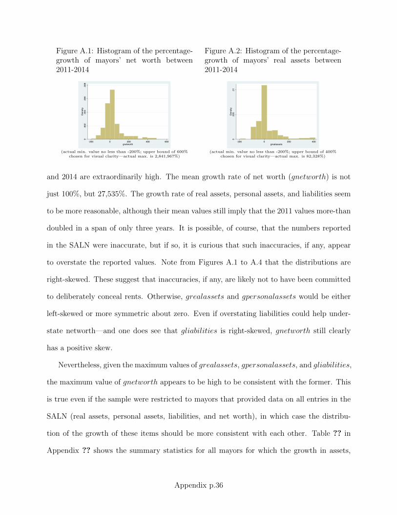
Figure A.1: Histogram of the percentage-growth of mayors’ net worth between2011-2014

0.002

.004

.006

.008

Density

-200 0 200 400 600gnetworth

(actual min. value no less than -200%; upper bound of 600%chosen for visual clarity—actual max. is 2,841,967%)

Figure A.2: Histogram of the percentage-growth of mayors’ real assets between2011-2014

0.005

.01

Density

-200 0 200 400grealassets

(actual min. value no less than -200%; upper bound of 400%chosen for visual clarity—actual max. is 82,328%)

and 2014 are extraordinarily high. The mean growth rate of net worth (gnetworth) is not

just 100%, but 27,535%. The growth rate of real assets, personal assets, and liabilities seem

to be more reasonable, although their mean values still imply that the 2011 values more-than

doubled in a span of only three years. It is possible, of course, that the numbers reported

in the SALN were inaccurate, but if so, it is curious that such inaccuracies, if any, appear

to overstate the reported values. Note from Figures A.1 to A.4 that the distributions are

right-skewed. These suggest that inaccuracies, if any, are likely not to have been committed

to deliberately conceal rents. Otherwise, grealassets and gpersonalassets would be either

left-skewed or more symmetric about zero. Even if overstating liabilities could help under-

state networth—and one does see that gliabilities is right-skewed, gnetworth still clearly

has a positive skew.

Nevertheless, given the maximum values of grealassets, gpersonalassets, and gliabilities,

the maximum value of gnetworth appears to be high to be consistent with the former. This

is true even if the sample were restricted to mayors that provided data on all entries in the

SALN (real assets, personal assets, liabilities, and net worth), in which case the distribu-

tion of the growth of these items should be more consistent with each other. Table ?? in

Appendix ?? shows the summary statistics for all mayors for which the growth in assets,

Appendix p.36

Figure A.3: Histogram of the percentage-growth of mayors’ personal assets be-tween 2011-2014

0.002

.004

.006

.008

.01

Density

-200 0 200 400 600gpersonalassets

(actual min. value no less than -100%; upper bound of 600%chosen for visual clarity—actual max. is 7,696%)

Figure A.4: Histogram of the percentage-growth of mayors’ liabilities between2011-2014

0.001

.002

.003

.004

.005

Density

-200 0 200 400 600gliabilities

(actual min. value no less than -200%; upper bound of 600%chosen for visual clarity—actual max. is 13,233%)

personal assets, liabilities and net worth are available and can be computed. (Growth rates

could not be obtained when the 2011 value is zero.) While the mean gnetworth drops consid-

erably to 17,176%, this still seems extraordinarily high, considering that the maximum value

of gnetworth remains at 2,841,967% while the maximum grealassets is only 82,327% and

maximum personalassets is only 7696%. One could thus try to restrict the sample based on

the value of gnetworth. Table ?? reports the summary statistics of the growth rates when

gnetworth is restricted to values: less than 1,000,000%, which removes one outlier; less than

1,000%, which removes another; and less than 100%, which removes an additional 27.

Note that while gnetworth drops considerably as more extreme values are removed, the

distribution of the other variables remain more or less stable, with the same minimum and

maximum values, and the mean values hovering around the same values. This is not to

be taken as evidence, however, that reported real assets, personal assets and liabilities are

any more accurate than reported net worth. In fact, if we were to exclude outliers based on

grealassets, or on gpersonalassets, or on gliabilities, the distribution of gnetworth remains

stable—its minimum and maximum values are the same, while the mean stays around 17,000

to 20,000%. (See Tables ?? and ??.)

Nevertheless, there does appear to be inaccuracies in the reported values. By identity,

Appendix p.37

net worth should be equal to the sum of real and personal assets, less liabilities. This implies

that the difference in net worth between 2011 and 2014 should also be equal to the sum of the

difference in real assets and difference in personal assets, minus the difference in liabilities.

However, this equality holds for only 89 out of the 231 mayors in the sample. This is not

to say that reported net worth are unreliable—it could be its components that have been

inaccurately reported such that some real and personal assets and liabilities were not listed,

even though the true net value (net worth) is provided. In fact, in Tables ?? and ??, while

the mean gnetworth seems consistent with the mean values of grealassets, gpersonalassets

and gliabilities when the reported net worth tallies with the calculated net worth based

on reported components, it is telling that when they do not match, gnetworth appears to

vastly outstrip the growth in real assets and real properties (net the growth in liabilities).

This suggests that some components of net worth might have been omitted. Yet despite

this apparent inaccuracy, recall that the distributions of grealassets and gpersonalassets

themselves are right-skewed (and gliabilities left-skewed), which suggest that real and per-

sonal assets are more likely overstated, than understated. It thus remains doubtful that any

inaccuracies in reporting might have been committed to deliberately conceal rents.30

To further strengthen the plausibility of this argument, Table ?? shows that mean

gnetworth is much larger for mayors with business interests than for those that do not.

Thus, it could simply be that the growth of mayors’ assets, liabilities and net worth were

simply fueled by their (legitimate) business activities. However, the business activities them-

selves could act as cover for rent-seeking. Concealment of rents might be less necessary if

a mayor has businesses that can legitimately generate additional income. Thus, a priori, it

is difficult to ascertain which outliers, if any, should be discarded from the sample, as they

30In Appendix ??, I present a model in which the politician’s decision to submit the SALN alreadyinternalizes her decision whether to (deliberately) report items in the SALN accurately or not. To the extentthat this model holds, any apparent inaccuracy that is revealed in the sample should be random, rather thanorchestrated.

Appendix p.38

might accurately report large rents. So as not to throw out observations that may very

well contain valuable information, the succeeding regressions use all 231 data points in the

sample.

9 Percentage growth of mayors’ assets and liabilities

Table A.10: Summary statistics for all mayors for whose percentage growth in net worth,real assets, personal assets, and liabilities can all be computed

(1) (2) (3) (4) (5)VARIABLES N mean sd min max

Percentage Growth of Net Worth 167 17,176 219,908 -196.2 2.842e+06Percentage Growth of Real Assets 167 520.8 6,370 -193.5 82,328Percentage Growth of Personal Assets 167 138.0 639.2 -100 7,696Percentage Growth of Liabilities 167 204.8 1,169 -168.6 13,233

10 Robustness Checks

I perform a number of robustness checks summarized below. Details are given in section ??.

Other proxies for spending g1S

The structural model implies that the exact same direct,

indirect and total effects should be obtained when using other components of total public

spending, e.g. spending on health, education, etc., since these components are actually jointly

determined. (See section ?? for a formal exposition.) This artifact of the model is confirmed

by the data—re-estimating the structural model using each of these other components of

total spending as alternative proxies for g1S

produces exactly the same direct, indirect, and

total effects.

Appendix p.39

Table A.11: Summary statistics for all mayors in ?? for whose percentage growth of networth is less than 1,000,000, less than 1,000, and less than 100, respectively

(1) (2) (3) (4) (5)VARIABLES N mean sd min max

Percentage Growth of Net Worth 166 159.6 1,049 -196.2 11,713Percentage Growth of Real Assets 166 524.3 6,389 -193.5 82,328Percentage Growth of Personal Assets 166 139.3 640.9 -100 7,696Percentage Growth of Liabilities 166 206.7 1,172 -168.6 13,233

(1) (2) (3) (4) (5)VARIABLES N mean sd min max

Percentage Growth of Net Worth 165 89.53 537.2 -196.2 6,720Percentage Growth of Real Assets 165 527.5 6,409 -193.5 82,328Percentage Growth of Personal Assets 165 140.1 642.8 -100 7,696Percentage Growth of Liabilities 165 208.2 1,176 -168.6 13,233

(1) (2) (3) (4) (5)VARIABLES N mean sd min max

Percentage Growth of Net Worth 137 1.366 45.88 -196.2 98.73Percentage Growth of Real Assets 137 618.0 7,034 -193.5 82,328Percentage Growth of Personal Assets 137 107.5 676.5 -100 7,696Percentage Growth of Liabilities 137 192.1 1,255 -168.6 13,233

Inclusion of NCR When the municipalities of the National Capital Region (NCR)/ Metro

Manila are included in the sample, the reduced-form regressions reveal the same pattern—

the IRA decreases the change in net worth (per spending). However, the estimated total

effect (from the structural model) of the IRA is now positive. For a municipality with mean

IRA, a 1-unit increase in the IRA i.e. an additional P 1 million, increases a mayor’s rents by

P 145.72m× (0.0000404) = P 5, 887.08. Nevertheless, the direct effect is still positive, which

reveals an increase in the rents from theft, while the indirect effect is still negative, which

implies a decrease in bribe payments, albeit the latter is sufficiently small in absolute value

such that it is exceeded by the latter. Figure 3 illustrates the effects for a municipality with

Appendix p.40

Table A.12: Summary statistics for all mayors in ?? for whose percentage growth of realassets is less than 50,000, less than 5,000, less than 500, and less than 100, respectively

(1) (2) (3) (4) (5)VARIABLES N mean sd min max

Percentage Growth of Net Worth 166 17,280 220,569 -196.2 2.842e+06Percentage Growth of Real Assets 166 27.97 151.5 -193.5 1,502Percentage Growth of Personal Assets 166 138.9 641.0 -100 7,696Percentage Growth of Liabilities 166 206.3 1,172 -168.6 13,233

(1) (2) (3) (4) (5)VARIABLES N mean sd min max

Percentage Growth of Net Worth 166 17,280 220,569 -196.2 2.842e+06Percentage Growth of Real Assets 166 27.97 151.5 -193.5 1,502Percentage Growth of Personal Assets 166 138.9 641.0 -100 7,696Percentage Growth of Liabilities 166 206.3 1,172 -168.6 13,233

(1) (2) (3) (4) (5)VARIABLES N mean sd min max

Percentage Growth of Net Worth 164 17,450 221,913 -196.2 2.842e+06Percentage Growth of Real Assets 164 15.19 85.75 -193.5 411.3Percentage Growth of Personal Assets 164 129.1 638.4 -100 7,696Percentage Growth of Liabilities 164 206.3 1,179 -168.6 13,233

(1) (2) (3) (4) (5)VARIABLES N mean sd min max

Percentage Growth of Net Worth 146 19,587 235,195 -196.2 2.842e+06Percentage Growth of Real Assets 146 -8.266 43.43 -193.5 89.94Percentage Growth of Personal Assets 146 130.0 673.1 -100 7,696Percentage Growth of Liabilities 146 197.6 1,241 -168.6 13,233

mean IRA.

Removal of Outliers Among the municipalities outside the NCR, the estimated effects

of the IRA on the change in net worth (per spending) appears to be (qualitatively) robust to

the removal of outliers. The direct effect remains positive, and the indirect effect negative.

Appendix p.41

Table A.13: Summary statistics for all mayors in ?? for whose percentage growth of personalassets is less than 5,000, and less than 100, respectively

(1) (2) (3) (4) (5)VARIABLES N mean sd min max

Percentage Growth of Net Worth 166 17,280 220,569 -196.2 2.842e+06Percentage Growth of Real Assets 166 524.3 6,389 -193.5 82,328Percentage Growth of Personal Assets 166 92.50 250.4 -100 1,676Percentage Growth of Liabilities 166 206.7 1,172 -168.6 13,233

(1) (2) (3) (4) (5)VARIABLES N mean sd min max

Percentage Growth of Net Worth 126 22,679 253,174 -100 2.842e+06Percentage Growth of Real Assets 126 670.1 7,333 -100 82,328Percentage Growth of Personal Assets 126 2.296 43.58 -100 99.96Percentage Growth of Liabilities 126 211.1 1,319 -100 13,233

Table A.14: Summary statistics for all mayors in ?? whose reported net worth tallies withcalculated net worth

(1) (2) (3) (4) (5)VARIABLES N mean sd min max

Percentage Growth of Net Worth 72 126.9 795.2 -100 6,720Percentage Growth of Real Assets 72 21.20 98.31 -100 650Percentage Growth of Personal Assets 72 206.8 934.7 -100 7,696Percentage Growth of Liabilities 72 280.9 1,587 -100 13,233

Table A.15: Summary statistics for all mayors in ?? whose reported net worth does not tallywith calculated net worth

(1) (2) (3) (4) (5)VARIABLES N mean sd min max

Percentage Growth of Net Worth 95 30,098 291,563 -196.2 2.842e+06Percentage Growth of Real Assets 95 899.4 8,445 -193.5 82,328Percentage Growth of Personal Assets 95 85.93 234.9 -100 1,583Percentage Growth of Liabilities 95 147.2 710.0 -168.6 6,236

Appendix p.42

Table A.16: Summary statistics for all mayors in ?? with business interests, and withoutbusiness interests, respectively

(1) (2) (3) (4) (5)VARIABLES N mean sd min max

Percentage Growth of Net Worth 100 28,599 284,181 -100 2.842e+06Percentage Growth of Real Assets 100 26.99 169.5 -100 1,502Percentage Growth of Personal Assets 100 102.2 286.5 -100 1,676Percentage Growth of Liabilities 100 266.8 1,373 -100 13,233

(1) (2) (3) (4) (5)VARIABLES N mean sd min max

Percentage Growth of Net Worth 67 128.2 824.0 -196.2 6,720Percentage Growth of Real Assets 67 1,258 10,055 -193.5 82,328Percentage Growth of Personal Assets 67 191.6 948.4 -99.05 7,696Percentage Growth of Liabilities 67 112.4 771.5 -168.6 6,236

Figure A.5: The effect of increasing the Internal Revenue Allotment (ira) by P 1 millionon theft, public spending, and bribe payments, simulated for a municipality with mean ira;sample includes NCR

1, 000, 000 =

{15, 271.46 stolen

984, 728.54 spent→ 9, 398.94 decrease in bribes

Total rents change by (15, 271.46− 9, 398.94) = 5, 872.52

However, Figure 4 shows that when the change in networth (per spending) is restricted to

values between −3 and 3, the indirect effect is smaller in absolute magnitude than the direct

effect, which generates a positive total effect. Figure 5 and 6 illustrates the case when the

change in real assets (per spending) is restricted between −0.5 and 0.5, and when the change

in liabilities (per spending) is between −0.2 and 0.2, respectively. In both cases, the the

indirect effect is sufficiently large such that the total effects are negative.

When the sample is further restricted to municipalities whose mayor’s change in net

worth (per spending) is between −0.2 and 0.2 (which removes 46 municipalities—about 20%

Appendix p.43

Figure A.6: The effect of increasing the Internal Revenue Allotment (ira) by P 1 millionon theft, public spending, and bribe payments, simulated for a municipality with meanira; sample includes only municipalities whose mayor’s change in net worth per spending isbetween −3 and 3

1, 000, 000 =

{18, 666.73 stolen

981, 333.27 spent→ 15, 038.30 decrease in bribes

Total rents change by (18, 666.73− 15, 038.30) = 3, 628.43

Figure A.7: The effect of increasing the Internal Revenue Allotment (ira) by P 1 millionon theft, public spending, and bribe payments, simulated for a municipality with mean ira;sample includes only municipalities whose mayor’s change in real assets per spending isbetween −0.5 to 0.5

1, 000, 000 =

{3, 395.28 stolen

996, 604.72 spent→ 20, 342.51 decrease in bribes

Total rents change by (3, 395.28− 20, 342.51) = −16, 947.24

Figure A.8: The effect of increasing the Internal Revenue Allotment (ira) by P 1 millionon theft, public spending, and bribe payments, simulated for a municipality with meanira; sample includes only municipalities whose mayor’s change in liabilities per spending isbetween −0.2 to 0.2

1, 000, 000 =

{17, 500.97 stolen

982, 499.03 spent→ 27, 613.94 decrease in bribes

Total rents change by (17, 500.97− 27, 613.94) = −10, 112.97

of the sample), it appears that revenues actually decrease (both types of) corruption. Both

the direct and indirect effects are negative, which implies that the marginal rents from theft

and from bribe payments decrease. From Figure 7, an additional P 1 million in IRA would

induce the mayor to ‘return’ or spend previously acquired rents equal to P 2, 506.38, such

that additional spending equals P 1, 002, 506.38. Such spending decreases bribe payments

Appendix p.44

by P 3, 016.40. Total rents thus decrease by 2, 506.38 + 3, 016.40 = P 5, 522.78. The finding

suggests that corruption is driven by the outliers in the sample. This, however, is to be

expected, since accumulated net worths close to zero are likely to capture growth in legitimate

wealth.

Figure A.9: The effect of increasing the Internal Revenue Allotment (ira) by P 1 millionon theft, public spending, and bribe payments, simulated for a municipality with meanira; sample includes only municipalities whose mayor’s change in net worth per spending isbetween −0.2 to 0.2

1, 000, 000 =

{2, 506.38 stolen

1, 002, 506.38 spent→ 3, 016.40 decrease in bribes

Total rents change by (−2, 506.38− 3, 016.40) = −5, 522.78

Allocated IRA The IRA data, as compiled by the Bureau of Local Government and

Finance, are the amounts that are reported to have been received by the municipalities. As

an alternative data source, the Department of Budget and Management (DBM) computes

the IRA that the national government allocates to each municipality, according to a fixed

formula specified by law. There are some discrepancies between the reported allocated and

reported received amounts—among the 231 municipalities in the sample, the mean received

IRA is P 98.52 million, while the mean allocated IRA is P 98.36 million. Nevertheless, re-

running the reduced-form regressions using the allocated IRA data generates almost identical

estimates. The estimated direct, indirect, and total effects are also very similar (See Figure

8.)

Note, however, that there are 92 municipalities, or about 40% of the sample, whose

received IRA is not equal to the allocated IRA. When these municipalities are dropped from

the sample, the total effect becomes positive. (See Figure 9.)

Appendix p.45

Figure A.10: The effect of increasing the Internal Revenue Allotment (ira) by P 1 millionon theft, public spending, and bribe payments, simulated for a municipality with mean ira;sample uses data on ira that has been allocated by the DBM

1, 000, 000 =

{18, 666.73 stolen

981, 333.27 spent→ 27, 715.94 decrease in bribes

Total rents change by (18, 666.73− 27, 715.94) = −9, 049.21

Figure A.11: The effect of increasing the Internal Revenue Allotment (ira) by P 1 millionon theft, public spending, and bribe payments, simulated for a municipality with meanira; sample includes only municipalities whose reported ira is exactly equal to the amountallocated by the DBM

1, 000, 000 =

{62, 470.16 stolen

937, 529.84 spent→ 43, 337.13 decrease in bribes

Total rents change by (62, 470.16− 43, 337.13) = 19, 133.03

Other proxies for d

Figure A.12: The effect of increasing the Internal Revenue Allotment (ira) by P 1 millionon theft, public spending, and bribe payments, simulated for a municipality with mean ira;sample uses data on city as proxy for whether or not the no-theft constraint binds

1, 000, 000 =

{100, 182.50 stolen

899, 817.50 spent→ 7, 796.02 decrease in bribes

Total rents change by (100, 182.50− 7, 796.02) = 92, 386.48

Lastly, I consider two other proxies for d—the variable that indicates whether the no-

theft constraint is binding. One is city, an indicator for city-municipalities, and another is

urban, an indicator for urban municipalities. It is reasonable to suppose that the no-theft

constraint is binding in cities and urban areas because there would be greater accountability

for public funds in these places. It would be harder to disguise theft since public projects

Appendix p.46

Figure A.13: The effect of increasing the Internal Revenue Allotment (ira) by P 1 millionon theft, public spending, and bribe payments, simulated for a municipality with mean ira;sample uses data on urban as proxy for whether or not the no-theft constraint binds

1, 000, 000 =

{312, 409.11 stolen

687, 590.89 spent→ 29, 566.59 decrease in bribes

Total rents change by (312, 409.11− 29, 566.59) = 282, 842.52

are more visible and vulnerable to scrutiny in dense areas.31 Using either of these proxies

generates a positive total effect of the IRA on the change in net worth (per spending), with

the direct effect still positive, and the indirect effect still negative. Figures 10 and 11 reveal

that the direct and total effects are much larger than when No Debt is used as proxy for d

(recall Figure 2), which suggests that the latter is a more conservative proxy for measuring

any increase in theft and total corruption.

11 Details of Robustness Checks

A Other proxies for spending g1S

Recall from the model that the direct effect D is unaffected by spending. This means that

using different proxies for g1S

should give the exact same estimate D. Furthermore, equations

(2) and (3) show that g1S

already incorporates g2—precisely by dividing by total spending

S, one knows that g1S

captures all other spending g2. That is, the components of total

spending are jointly determined. In what follows, I show that the indirect effect I is the

same, regardless of which component is used to proxy for g1S

. Thus, one does not need to

know ex-ante which type of public spending generates bribes—the same indirect effect I is

31Technically, however, these proxies do not/cannot be caused by revenues and λ, although they may becorrelated with them. For this reason, No Debt is still the most conceptually suitable proxy.

Appendix p.47

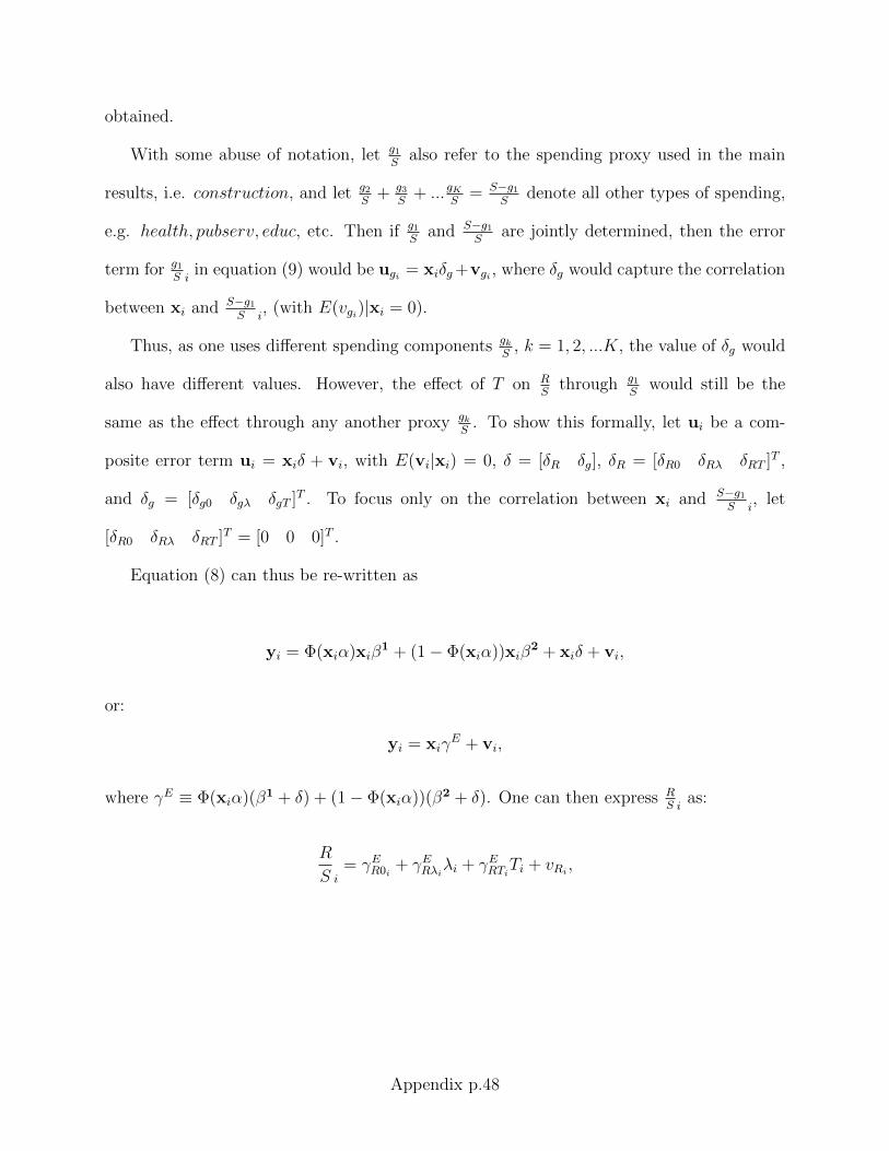
obtained.

With some abuse of notation, let g1S

also refer to the spending proxy used in the main

results, i.e. construction, and let g2S

+ g3S

+ ...gKS

= S−g1S

denote all other types of spending,

e.g. health, pubserv, educ, etc. Then if g1S

and S−g1S

are jointly determined, then the error

term for g1S i

in equation (9) would be ugi = xiδg+vgi , where δg would capture the correlation

between xi and S−g1S i

, (with E(vgi)|xi = 0).

Thus, as one uses different spending components gkS

, k = 1, 2, ...K, the value of δg would

also have different values. However, the effect of T on RS

through g1S

would still be the

same as the effect through any another proxy gkS

. To show this formally, let ui be a com-

posite error term ui = xiδ + vi, with E(vi|xi) = 0, δ = [δR δg], δR = [δR0 δRλ δRT ]T ,

and δg = [δg0 δgλ δgT ]T . To focus only on the correlation between xi and S−g1S i

, let

[δR0 δRλ δRT ]T = [0 0 0]T .

Equation (8) can thus be re-written as

yi = Φ(xiα)xiβ1 + (1− Φ(xiα))xiβ

2 + xiδ + vi,

or:

yi = xiγE + vi,

where γE ≡ Φ(xiα)(β1 + δ) + (1− Φ(xiα))(β2 + δ). One can then express RS i

as:

R

S i= γER0i

+ γERλiλi + γERTiTi + vRi ,

Appendix p.48

where:

γER0i= Φ(xiα)(β1

R0 + δR0) + (1− Φ(xiα))(β2R0 + δR0)

γERλi = Φ(xiα)(β1Rλ + δRλ) + (1− Φ(xiα))(β2

Rλ + δRλ),

γERTi = Φ(xiα)(β1RT + δRT ) + (1− Φ(xiα))(β2

RT + δRT ),

β1R = [β1

R0 β1Rλ β1

RT ]T and β2R = [β2

R0 β2Rλ β2

RT ]T .

(16)

However, with [δR0 δRλ δRT ]T = [0 0 0]T , this reduces to

R

S i= Φ(xiα)[(β1

R0 − β2R0) + (β1

Rλ − β2Rλ)λi + (β1

RT − β2RT )Ti] + β2

R0 + β2Rλλi + β2

RTTi + vRi .

Finally, since E(vi|xi) = 0, the expected value of RS i

given xi is the same as before (see

equation (12)):

E[(R

S i)|xi] = Φ(xiα)[(β1

R0 − β2R0) + (β1

Rλ − β2Rλ)λi + (β1

RT − β2RT )Ti] + β2

R0 + β2Rλλi + β2

RTTi,

as well as its derivative with respect to revenues (see equation (13)):

dE[(RS i

)|xi]dTi

= [Φ(xiα)+φ(xiα)αTTi](β1RT−β2

RT )+φ(xiα)αT [(β1R0−β2

R0)+(β1Rλ−β2

Rλ)λi]+β2RT ,

Thus, the same direct, indirect, and total effects are obtained, which implies that the partic-

ular choice of spending proxy, as long as it is divided by total spending S, is inconsequential.

Indeed, Tables ?? to ?? show that using different components of spending gives the exact

Appendix p.49

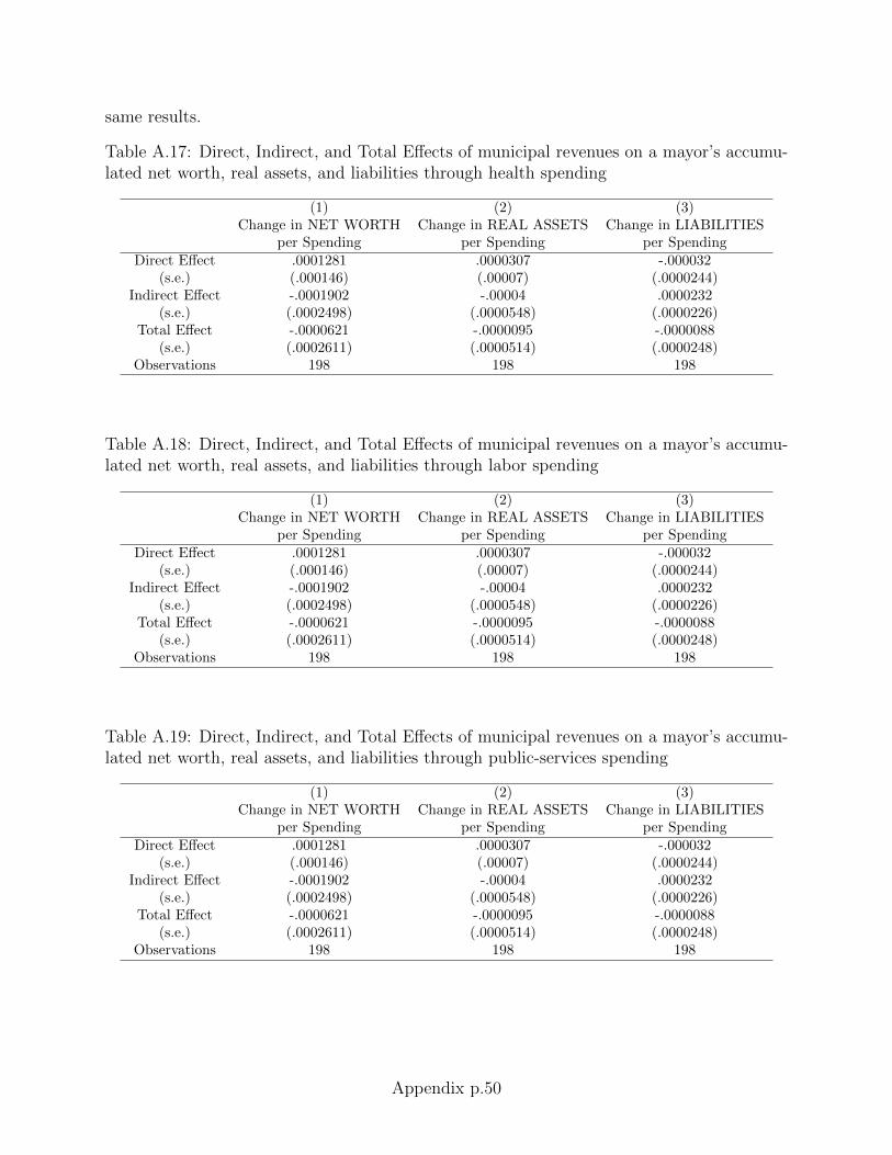
same results.

Table A.17: Direct, Indirect, and Total Effects of municipal revenues on a mayor’s accumu-lated net worth, real assets, and liabilities through health spending

(1) (2) (3)Change in NET WORTH Change in REAL ASSETS Change in LIABILITIES

per Spending per Spending per SpendingDirect Effect .0001281 .0000307 -.000032

(s.e.) (.000146) (.00007) (.0000244)Indirect Effect -.0001902 -.00004 .0000232

(s.e.) (.0002498) (.0000548) (.0000226)Total Effect -.0000621 -.0000095 -.0000088

(s.e.) (.0002611) (.0000514) (.0000248)Observations 198 198 198

Table A.18: Direct, Indirect, and Total Effects of municipal revenues on a mayor’s accumu-lated net worth, real assets, and liabilities through labor spending

(1) (2) (3)Change in NET WORTH Change in REAL ASSETS Change in LIABILITIES

per Spending per Spending per SpendingDirect Effect .0001281 .0000307 -.000032

(s.e.) (.000146) (.00007) (.0000244)Indirect Effect -.0001902 -.00004 .0000232

(s.e.) (.0002498) (.0000548) (.0000226)Total Effect -.0000621 -.0000095 -.0000088

(s.e.) (.0002611) (.0000514) (.0000248)Observations 198 198 198

Table A.19: Direct, Indirect, and Total Effects of municipal revenues on a mayor’s accumu-lated net worth, real assets, and liabilities through public-services spending

(1) (2) (3)Change in NET WORTH Change in REAL ASSETS Change in LIABILITIES

per Spending per Spending per SpendingDirect Effect .0001281 .0000307 -.000032

(s.e.) (.000146) (.00007) (.0000244)Indirect Effect -.0001902 -.00004 .0000232

(s.e.) (.0002498) (.0000548) (.0000226)Total Effect -.0000621 -.0000095 -.0000088

(s.e.) (.0002611) (.0000514) (.0000248)Observations 198 198 198

Appendix p.50

Table A.20: Direct, Indirect, and Total Effects of municipal revenues on a mayor’s accumu-lated net worth, real assets, and liabilities through education spending

(1) (2) (3)Change in NET WORTH Change in REAL ASSETS Change in LIABILITIES

per Spending per Spending per SpendingDirect Effect .0001281 .0000307 -.000032

(s.e.) (.000146) (.00007) (.0000244)Indirect Effect -.0001902 -.00004 .0000232

(s.e.) (.0002498) (.0000548) (.0000226)Total Effect -.0000621 -.0000095 -.0000088

(s.e.) (.0002611) (.0000514) (.0000248)Observations 198 198 198

Table A.21: Direct, Indirect, and Total Effects of municipal revenues on a mayor’s accumu-lated net worth, real assets, and liabilities through social welfare spending

(1) (2) (3)Change in NET WORTH Change in REAL ASSETS Change in LIABILITIES

per Spending per Spending per SpendingDirect Effect .0001281 .0000307 -.000032

(s.e.) (.000146) (.00007) (.0000244)Indirect Effect -.0001902 -.00004 .0000232

(s.e.) (.0002498) (.0000548) (.0000226)Total Effect -.0000621 -.0000095 -.0000088

(s.e.) (.0002611) (.0000514) (.0000248)Observations 198 198 198

Table A.22: Direct, Indirect, and Total Effects of municipal revenues on a mayor’s accumu-lated net worth, real assets, and liabilities through economic services spending

(1) (2) (3)Change in NET WORTH Change in REAL ASSETS Change in LIABILITIES

per Spending per Spending per SpendingDirect Effect .0001281 .0000307 -.000032

(s.e.) (.000146) (.00007) (.0000244)Indirect Effect -.0001902 -.00004 .0000232

(s.e.) (.0002498) (.0000548) (.0000226)Total Effect -.0000621 -.0000095 -.0000088

(s.e.) (.0002611) (.0000514) (.0000248)Observations 198 198 198

B Inclusion of NCR mayors

Table ?? estimates the reduced-form model, while Table ?? estimates the structural model,

using a sample that includes municipalities from NCR/Metro Manila.

Appendix p.51

Table A.23: Total effect of IRA on mayor’s accumulated net worth, real assets, and liabilities,by quantile regression—sample includes NCR

(1) (2) (3) (4) (5) (6)Change in NETWORTH Change in REAL ASSETS Change in LIABILITIES

per Spending per Spending per Spending

Proportion of Population Aged 15-24 -0.103 -0.00524 -0.00360(0.140) (0.0375) (0.0448)

Internal Revenue Allotment -7.06e-06* -4.40e-06 0 3.03e-08 0 -7.99e-08(3.69e-06) (1.51e-05) (5.63e-07) (4.39e-06) (3.54e-06) (4.31e-06)

Constant 0.00778*** 0.0271 0 0.00110 0 0.000744(0.00192) (0.0273) (0.000587) (0.00725) (0.000892) (0.00869)

Observations 241 208 231 198 231 198sum adev 12.38 10.36 4.424 3.753 2.644 2.153sum rdev 12.39 10.37 4.424 3.754 2.644 2.153

Robust standard errors in parentheses*** p<0.01, ** p<0.05, * p<0.1

Table A.24: Direct, Indirect, and Total Effects of municipal revenues on a mayor’s accumu-lated net worth, real assets, and liabilities through construction spending; sample includesNCR

(1) (2) (3)Change in NET WORTH Change in REAL ASSETS Change in LIABILITIES

per Spending per Spending per SpendingDirect Effect .0001048 .0000307 -.000032

(s.e.) (.0001077) (.0000725) (.0000225)Indirect Effect -.0000645 -.0000315 .000014

(s.e.) (.0001181) (.0000459) (.0000207)Total Effect .0000404 .0000008 -.000018

(s.e.) (.0001265) (.0000572) (.0000235)Observations 208 208 208

C Removal of Outliers

Figures A.5a–c reveal that except for few values that are very far from zero, the distributions

of networth, realassets and liabilities are symmetric about zero. I drop these extreme values

and re-estimate the structural model. Table ?? reports results for the case when networth

is restricted to values between −3 and 3, Table ?? for when realassets is between −0.5 and

0.5, Table ?? for when liabilities is between −0.2 and 0.2, and Table ?? for when networth

Appendix p.52

is further restricted to values between −0.2 and 0.2.

Figure A.14: Kdensity Plots

0.5

11.

52

2.5

Den

sity

-5 0 5 10networth

kernel = epanechnikov, bandwidth = 0.0086

Kernel density estimate

(a) networth ∈ (−3, 3) approx. symmetric around zero

02

46

Den

sity

-1.5 -1 -.5 0 .5realassets

kernel = epanechnikov, bandwidth = 0.0039

Kernel density estimate

(b) realassets ∈ (−0.5, 0.5) approx. symmetricaround zero

010

2030

Den

sity

-.4 -.2 0 .2liabilities

kernel = epanechnikov, bandwidth = 0.0029

Kernel density estimate

(c) liabilities ∈ (−0.2, 0.2) approx. symmetricaround zero

Table A.25: Direct, Indirect, and Total Effects of municipal revenues on a mayor’s accumu-lated net worth, real assets, and liabilities through construction spending; sample includesonly municipalities whose mayor’s change in net worth per spending is between −3 and 3

(1) (2) (3)Change in NET WORTH Change in REAL ASSETS Change in LIABILITIES

per Spending per Spending per SpendingDirect Effect .0001281 .0000307 -.000032

(s.e.) (.0001418) (.0000699) (.0000229)Indirect Effect -.0001032 -.0000387 .0000213

(s.e.) (.0000864) (.0000541) (.0000223)Total Effect .0000249 -.0000081 -.0000107

(s.e.) (.0000962) (.0000558) (.0000230)Observations 197 197 197

Appendix p.53

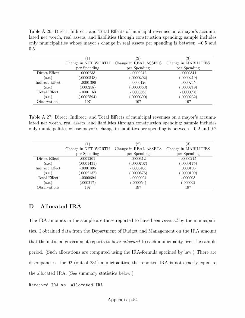
Table A.26: Direct, Indirect, and Total Effects of municipal revenues on a mayor’s accumu-lated net worth, real assets, and liabilities through construction spending; sample includesonly municipalities whose mayor’s change in real assets per spending is between −0.5 and0.5

(1) (2) (3)Change in NET WORTH Change in REAL ASSETS Change in LIABILITIES

per Spending per Spending per SpendingDirect Effect .0000233 -.0000242 -.0000341

(s.e.) (.0000548) (.0000292) (.0000219)Indirect Effect -.0001396 -.0000126 .0000245

(s.e.) (.000258) (.0000368) (.0000219)Total Effect -.0001163 -.0000368 -.0000096

(s.e.) (.0002594) (.0000390) (.0000232)Observations 197 197 197

Table A.27: Direct, Indirect, and Total Effects of municipal revenues on a mayor’s accumu-lated net worth, real assets, and liabilities through construction spending; sample includesonly municipalities whose mayor’s change in liabilities per spending is between −0.2 and 0.2

(1) (2) (3)Change in NET WORTH Change in REAL ASSETS Change in LIABILITIES

per Spending per Spending per SpendingDirect Effect .0001201 .0000312 -.0000215

(s.e.) (.0001431) (.0000707) (.0000175)Indirect Effect -.0001895 -.0000406 .0000185

(s.e.) (.0002137) (.0000575) (.0000199)Total Effect -.0000694 -.0000094 -.000003

(s.e.) (.000217) (.000054) (.00002)Observations 197 197 197

D Allocated IRA

The IRA amounts in the sample are those reported to have been received by the municipali-

ties. I obtained data from the Department of Budget and Management on the IRA amount

that the national government reports to have allocated to each municipality over the sample

period. (Such allocations are computed using the IRA-formula specified by law.) There are

discrepancies—for 92 (out of 231) municipalities, the reported IRA is not exactly equal to

the allocated IRA. (See summary statistics below.)

Received IRA vs. Allocated IRA

Appendix p.54

Table A.28: Direct, Indirect, and Total Effects of municipal revenues on a mayor’s accumu-lated net worth, real assets, and liabilities through construction spending; sample includesonly municipalities whose mayor’s change in net worth per spending is between −0.2 and0.2

(1) (2) (3)Change in NET WORTH Change in REAL ASSETS Change in LIABILITIES

per Spending per Spending per SpendingDirect Effect -.0000172 -.0000255 -.0000255

(s.e.) (.000028) (.0000268) (.0000171)Indirect Effect -.0000207 .0000005 .0000154

(s.e.) (.0000265) (.00003) (.0000206)Total Effect -.0000379 -.000025 -.0000101

(s.e.) (.0000291) (.0000316) (.0000215)Observations 185 185 185

Variable | Obs Mean Std. Dev. Min Max

-------------+---------------------------------------------------------

Received IRA | 231 98.52139 119.839 24.29 1083.83

Allocated IRA | 231 98.35736 118.5756 24.29 1062.27

However, Tables ?? to ?? show that using the allocated IRA in lieu of the received IRAgenerates estimates that are practically identical to estimates using received IRA.

Table A.29: Estimating the probability (by probit regression) that the no-theft constraintbinds, as proxied by No Debt; revenues proxied by allocated Internal Revenue Allotment

VARIABLES No Debt

Proportion of Population Aged 15-24 4.663(6.013)

Internal Revenue Allotment (Allocated) -0.00190**(0.000963)

Constant -1.133(1.163)

Observations 198Standard errors in parentheses

*** p<0.01, ** p<0.05, * p<0.1

When the municipalities whose received IRA is not equal to allocated IRA are droppedfrom the sample, the results are different—while the direct effect is still positive, and theindirect effect still negative, the total effect is now positive (See Table ??.)

Appendix p.55

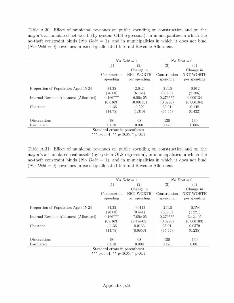
Table A.30: Effect of municipal revenues on public spending on construction and on themayor’s accumulated net worth (by system OLS regression), in municipalities in which theno-theft constraint binds (No Debt = 1), and in municipalities in which it does not bind(No Debt = 0); revenues proxied by allocated Internal Revenue Allotment

No Debt = 1 No Debt = 0(1) (2) (3) (4)

Change in Change inConstruction NET WORTH Construction NET WORTH

spending per spending spending per spending

Proportion of Population Aged 15-24 34.35 2.042 -211.5 -0.912(76.08) (6.754) (339.3) (2.186)

Internal Revenue Allotment (Allocated) 0.166*** -6.50e-05 0.276*** 0.000134(0.0163) (0.00145) (0.0286) (0.000184)

Constant -11.36 -0.229 35.01 0.148(14.75) (1.310) (65.45) (0.422)

Observations 68 68 130 130R-squared 0.618 0.001 0.425 0.005

Standard errors in parentheses*** p<0.01, ** p<0.05, * p<0.1

Table A.31: Effect of municipal revenues on public spending on construction and on themayor’s accumulated real assets (by system OLS regression), in municipalities in which theno-theft constraint binds (No Debt = 1), and in municipalities in which it does not bind(No Debt = 0); revenues proxied by allocated Internal Revenue Allotment

No Debt = 1 No Debt = 0(1) (2) (3) (4)

Change in Change inConstruction NET WORTH Construction NET WORTH

spending per spending spending per spending

Proportion of Population Aged 15-24 34.35 -0.0113 -211.5 -0.358(76.08) (0.441) (339.3) (1.221)

Internal Revenue Allotment (Allocated) 0.166*** -7.05e-05 0.276*** 3.42e-05(0.0163) (9.47e-05) (0.0286) (0.000103)

Constant -11.36 0.0133 35.01 0.0579(14.75) (0.0856) (65.45) (0.235)

Observations 68 68 130 130R-squared 0.618 0.009 0.425 0.001

Standard errors in parentheses*** p<0.01, ** p<0.05, * p<0.1

Appendix p.56

Table A.32: Effect of municipal revenues on public spending on construction and on themayor’s accumulated liabilities (by system OLS regression), in municipalities in which theno-theft constraint binds (No Debt = 1), and in municipalities in which it does not bind(No Debt = 0); revenues proxied by allocated Internal Revenue Allotment

No Debt = 1 No Debt = 0(1) (2) (3) (4)

Change in Change inConstruction NET WORTH Construction NET WORTH

spending per spending spending per spending

Proportion of Population Aged 15-24 34.35 0.00741 -211.5 0.130(76.08) (0.222) (339.3) (0.368)

Internal Revenue Allotment (Allocated) 0.166*** 1.13e-05 0.276*** -3.29e-05(0.0163) (4.77e-05) (0.0286) (3.10e-05)

Constant -11.36 -0.00541 35.01 -0.0114(14.75) (0.0431) (65.45) (0.0710)

Observations 68 68 130 130R-squared 0.618 0.001 0.425 0.009

Standard errors in parentheses*** p<0.01, ** p<0.05, * p<0.1

Table A.33: Direct, Indirect, and Total Effects of municipal revenues on a mayor’s accumu-lated net worth, real assets, and liabilities through construction spending; revenues proxiedby allocated Internal Revenue Allotment

(1) (2) (3)Change in NET WORTH Change in REAL ASSETS Change in LIABILITIES

per Spending per Spending per SpendingDirect Effect .0001281 .0000307 -.000032

(s.e.) (.0001457) (.00007) (.0000244)Indirect Effect -.0001902 -.00004 .0000232

(s.e.) (.0002498) (.0000548) (.0000226)Total Effect -.0000621 -.0000094 -.0000088

(s.e.) (.0002611) (.0000514) (.0000248)Observations 198 198 198

E Other proxies for d

Lastly, I use two other proxies for d (i.e. the indicator for when the no-theft constraintis binding), namely, city, an indicator for city-municipalities, and urban, an indicator forurban municipalities. As Tables ?? and ?? show, the estimated total effect (via the structuralapproach) is now positive, albeit the direct effect is still positive and the indirect effect stillnegative.

Appendix p.57

Table A.34: Direct, Indirect, and Total Effects of municipal revenues on a mayor’s accumu-lated net worth, real assets, and liabilities through construction spending; sample includesonly municipalities with received equal to allocated Internal Revenue Allotment

(1) (2) (3)Change in NET WORTH Change in REAL ASSETS Change in LIABILITIES

per Spending per Spending per SpendingDirect Effect .0004287 .0001173 -.0000578

(s.e.) (.000296) (.0001515) (.0000443)Indirect Effect -.0002974 -.0001454 (.000116)

(s.e.) (.0002215) (.0001282) (.0000531)Total Effect .0001312 -.000028 .0000582

(s.e.) (.0002263) (.0001277) (.0000547)Observations 113 113 113

Table A.35: Direct, Indirect, and Total Effects of municipal revenues on a mayor’s accumu-lated net worth, real assets, and liabilities through construction spending; no-theft constraintproxied by city

(1) (2) (3)Change in NET WORTH Change in REAL ASSETS Change in LIABILITIES

per Spending per Spending per SpendingDirect Effect .0006875 .0001247 -.0000305

(s.e.) (.0007139) (.0001851) (.0000641)Indirect Effect -.0000535 -.0000139 -.0000087

(s.e.) (.0001201) (.0000351) (.0000127)Total Effect .000634 .0001108 -.0000392

(s.e.) (.000652) (.0001741) (.0000624)Observations 198 198 198

Table A.36: Direct, Indirect, and Total Effects of municipal revenues on a mayor’s accumu-lated net worth, real assets, and liabilities through construction spending; no-theft constraintproxied by urban

(1) (2) (3)Change in NET WORTH Change in REAL ASSETS Change in LIABILITIES

per Spending per Spending per SpendingDirect Effect .0021439 .0003165 -.0000005

(s.e.) (0.000657) (.0003521) (.0001085)Indirect Effect -.0002029 -.0000336 -.0000068

(s.e.) (.0000784) (.0000177) (.0000085)Total Effect .001941 .0002829 -.0000073

(s.e.) (.0006031) (.0003373) (.0001033)Observations 198 198 198

12 Additional Tables

Appendix p.58

Table A.37: Direct, Indirect, and Total Effects of municipal revenues on a mayor’s accumu-lated net worth through construction spending, using different proxies for λ

Change in NET WORTH per Spending, using as λ the following proxies:Proportion Proportion Proportion Proportion Proportion

of School-Age Youth Who Are of Population of Households of Population whoEnrolled in School Employed in Professional Jobs That Have a Cellphone are Registered Voters

Direct Effect .0001057 .0001294 .0000596 .0001026 .0007989(s.e.) (.0001328) (.000135) (.0000975) (.0001307) (.0005053)

Indirect Effect -.0001342 -.0001702 -.0008474 -.0002589 .0010737(s.e.) (.0002666) (.0002569) (.0007179) (.0003786) (.0018987)

Total Effect -.0000285 -.0000408 -.0007879 -.0001563 .0018726(s.e.) (.0002742) (.0002606) (.0007209) (.0003854) (.0019048)

Observations 198 198 198 198 205

Table A.38: Direct, Indirect, and Total Effects of municipal revenues on a mayor’s accumu-lated net worth through construction spending, subsetting the sample of municipalities bymajor geographical areas Luzon, Visayas-Mindanao

Change in NET WORTH per Spending, using municipalities in:Entire country Luzon Visayas and

MindanaoDirect Effect .0001281 .0004345 -.0000065

(s.e.) (.0001457) (.0004249) (.0000508)Indirect Effect -.0001902 -.0003678 -.0000315

(s.e.) (.0002498) (.0008233) (.00005)Total Effect -.0000621 .0000667 -.0000381

(s.e.) (.0002611) (.0008281) (.0000612)Observations 198 129 69

Appendix p.59

Table A.39: Effect of municipal revenues on public spending on construction and on themayor’s accumulated net worth (by system OLS regression), in municipalities in which theno-theft constraint binds (No Debt = 1), and in municipalities in which it does not bind(No Debt = 0); sample includes only municipalities in Visayas and Mindanao

No Debt = 1 No Debt = 0(1) (2) (3) (4)

Change in Change inConstruction NET WORTH Construction NET WORTH

spending per spending spending per spending

Proportion of Population Aged 15-24 91.06 -1.299 -179.5 0.630(72.80) (0.953) (169.2) (0.784)

Internal Revenue Allotment 0.0857*** -4.93e-05 0.160*** -6.53e-06(0.0213) (0.000279) (0.0113) (5.22e-05)

Constant -20.82 0.294 33.18 -0.118(14.44) (0.189) (33.74) (0.156)

Observations 17 17 52 52R-squared 0.570 0.115 0.797 0.012

Standard errors in parentheses*** p<0.01, ** p<0.05, * p<0.1

Table A.40: Effect of municipal revenues on public spending on construction and on themayor’s accumulated net worth (by system OLS regression), in municipalities in which theno-theft constraint binds (No Debt = 1), and in municipalities in which it does not bind(No Debt = 0); sample includes only municipalities in Luzon

No Debt = 1 No Debt = 0(1) (2) (3) (4)

Change in Change inConstruction NET WORTH Construction NET WORTH

spending per spending spending per spending

Proportion of Population Aged 15-24 65.92 3.533 218.6 -5.185(89.78) (8.278) (559.6) (4.493)

Internal Revenue Allotment 0.167*** -0.000135 0.524*** 0.000435(0.0183) (0.00169) (0.0518) (0.000416)

Constant -16.16 -0.460 -65.15 0.915(17.19) (1.585) (105.5) (0.847)

Observations 51 51 78 78R-squared 0.639 0.004 0.592 0.024

Standard errors in parentheses*** p<0.01, ** p<0.05, * p<0.1

Appendix p.60

Table A.41: Direct, Indirect, and Total Effects of municipal revenues on the differences innet worth, real assets, and liabilities of the 2011 and the 2014 mayors through constructionspending; using placebo sample

(1) (2) (3)Difference in NET WORTH Difference in REAL ASSETS Difference in LIABILITIES

per Spending per Spending per SpendingDirect Effect .0003089 -.0000534 -.0000922

(s.e.) (.0003481) (.0000585) (.0000587)Indirect Effect -.0001304 -.000062 -.0001252

(s.e.) (.0002187) (.0001421) (.0001923)Total Effect .0001785 -.0001154 -.0002175

(s.e.) (.0001761) (.0001433) (.0001938)Observations 128 128 128

Table A.42: Estimating the probability (by probit regression) that the no-theft constraintbinds, as proxied by No Debt; using placebo sample

No DebtProportion of Population Aged 15-24 -3.950

(10.21)Internal Revenue Allotment -0.00235**

(0.00114)Constant 0.527

(1.983)Observations 128

Standard errors in parentheses*** p<0.01, ** p<0.05, * p<0.1

Appendix p.61

Table A.43: Effect of municipal revenues on public spending on construction and on thedifference in net worth of the 2011 and 2014 mayors (by system OLS regression), in munici-palities in which the no-theft constraint binds (No Debt = 1), and in municipalities in whichit does not bind (No Debt = 0); using placebo sample

No Debt = 1 No Debt = 0(1) (2) (3) (4)

Difference in Difference inConstruction NET WORTH Construction NET WORTH

spending per spending spending per spending

Proportion of Population Aged 15-24 -13.69 1.336 8.675 0.463(249.0) (2.961) (249.0) (8.447)

Internal Revenue Allotment 0.197*** 7.05e-05 0.191*** 0.000309(0.0281) (0.000334) (0.0196) (0.000666)

Constant -4.772 -0.289 -6.022 -0.223(48.49) (0.577) (48.37) (1.641)

Observations 39 39 89 89R-squared 0.558 0.006 0.523 0.003

Standard errors in parentheses*** p<0.01, ** p<0.05, * p<0.1

Table A.44: Effect of municipal revenues on public spending on construction and on thedifference in real assets of the 2011 and 2014 mayors (by system OLS regression), in mu-nicipalities in which the no-theft constraint binds (No Debt = 1), and in municipalities inwhich it does not bind (No Debt = 0); using placebo sample

No Debt = 1 No Debt = 0(1) (2) (3) (4)

Difference in Difference inConstruction REAL ASSETS Construction REAL ASSETS

spending per spending spending per spending

Proportion of Population Aged 15-24 -13.69 -0.600 8.675 -0.376(249.0) (7.395) (249.0) (1.205)

Internal Revenue Allotment 0.197*** -0.000199 0.191*** -5.34e-05(0.0281) (0.000835) (0.0196) (9.50e-05)

Constant -4.772 0.178 -6.022 0.0923(48.49) (1.440) (48.37) (0.234)

Observations 39 39 89 89R-squared 0.558 0.002 0.523 0.005

Standard errors in parentheses*** p<0.01, ** p<0.05, * p<0.1

Appendix p.62

Table A.45: Effect of municipal revenues on public spending on construction and on thedifference in liabilities of the 2011 and 2014 mayors (by system OLS regression), in munici-palities in which the no-theft constraint binds (No Debt = 1), and in municipalities in whichit does not bind (No Debt = 0); using placebo sample

No Debt = 1 No Debt = 0(1) (2) (3) (4)

Difference in Difference inConstruction LIABILITIES Construction LIABILITIES

spending per spending spending per spending

Proportion of Population Aged 15-24 -13.69 -2.196 8.675 -0.716(249.0) (10.24) (249.0) (1.154)

Internal Revenue Allotment 0.197*** -0.000388 0.191*** -9.22e-05(0.0281) (0.00116) (0.0196) (9.10e-05)

Constant -4.772 0.553 -6.022 0.180(48.49) (1.993) (48.37) (0.224)

Observations 39 39 89 89R-squared 0.558 0.004 0.523 0.018

Standard errors in parentheses*** p<0.01, ** p<0.05, * p<0.1

Appendix p.63