Gradual bidding in ebay-like auctions∗

Attila Ambrus† James Burns ‡ Yuhta Ishii §

May 22, 2012

This paper shows that in online auctions like eBay, if bidders are not con-tinuously participating in the auction but can only place bids at random times,then many different equilibria arise besides truthful bidding, despite the optionto leave proxy bids. These equilibria can involve gradual bidding, periods ofinactivity, and waiting to start bidding towards the end of the auction - biddingbehaviors common on eBay. In a common value environment, we characterizea class of equilibria that include the best and worst equilibria for the seller.The revenue of the seller in the latter can be a small fraction of what could beobtained at a sealed-bid second-price auction. For large number of bidders, weshow that the worst equilibrium has the feature that bidders are passive untilnear the end of the auction, and then they start bidding incrementally.

∗We thank Itay Fainmesser, Drew Fudenberg, Tanjim Hossain, Al Roth and seminar partic-ipants at Duke University, the Harvard-MIT theory seminar, University of Maryland, Wash-ington University and University of Pittsburgh for useful comments.

†Department of Economics, Duke University, Box 90097, Durham NC 27708,aa231@duke.edu

‡Department of Economics, Harvard University, Cambridge, MA 02138,jburns@fas.harvard.edu

§Department of Economics, Harvard University, Cambridge, MA 02138,ishii2@fas.harvard.edu

1

1 Introduction

A distinguishing feature of online auctions, relative to spot auctions, is thatthey typically last for a relatively long time.1 However, this aspect is oftensuppressed in the related economics literature. In particular, for bidders withprivate evaluations, online auction mechanisms such as eBay, where bidders canleave a proxy bid and the highest bidder wins the object at a price equal to thesecond highest bid (plus a minimum bid increment) are commonly regarded asstrategically equivalent to second-price sealed-bid auctions. Since bidding one’strue evaluation in the latter context is a weakly dominant strategy, and placinga bid takes some effort, the argument establishes that a rational bidder at aneBay-like auction should only place one bid, equal to her true evaluation, at herearliest convenience.

In contrast with the above predictions, observed bidding behavior on ebayinvolves both a substantial amount of gradual bidding and last-minute bidding(commonly referred to as sniping). Ockenfels and Roth (2006) report that theaverage number of bids per bidder is 1.89 and 38 % of bidders submit morethan one bid. In the field experiment of Hossain and Morgan (2006) 76 % ofthe auctions had at least one bidder placing multiple bids.2 Regarding sniping,Roth and Ockenfels (2002) report that 18% of auctions in their data receivedbids in the last minute, while Bajari and Hortacsu (2003) find that the medianwinning bid arrives after 98.3% of the auction time elapsed, while 25% of thewinning bids arrive after 99.8% of the auction time elapsed.

While Roth and Ockenfels (2002) proposes a model in which last-minute bid-ding can be an equilibrium,3 the existing literature typically considers gradualbidding to be a naive (irrational) behavior. Relatedly, Ku et al. (2005) explainbidding behavior on online auctions with a model of emotional decision-makingand competitive arousal, Ely and Hossain (2009) describe incremental biddersas confused, mistaking eBay’s proxy system for an ascending auction, whileHossain (2008) explains observed bidding behavior using behavioral buyers wholearn about their own valuations through the process of placing bids.4

1On eBay sellers can specify durations ranging from 1 day to 30 days.2See also Zeithammer and Adams (2010), who find evidence in online auction field data

for incremental bidding. For example they find that the frequency of the winning bid beingexactly the minimum increment higher than the runner up bid to be too high than what wouldbe implied by truthful bidding (they observe the winning bidder’s proxy bid, hence they canperform this test). Moreover, such an event is much more likely if the winning bidder placesa bid after the runner up bidder than vice versa.

3However, Hasker et al. (2009), using ebay data, reject the hypothesis that bidders followa war of snipe profile as in Roth and Ockenfels (2002). See also Ariely et al. (2005) for arelated laboratory experiment.

4See also Compte and Jehiel (2004) and Rasmusen (2006) for bidders learning their trueevaluations during the auction. Other explanations include the presence of multiple over-lapping auctions for identical or close substitute objects as in Peters and Severinov (2006),Hendricks et al. (2009), and Fu (2009). However, gradual and last-minute bidding seemsto be prevalent for rare or unique objects, too, not only for objects with many close substi-tutes being auctioned at any time (for example, they occur in the experiments of Ariely etal. (2005) despite there is no concurrent competing auction). Furthermore, as Hossain (2008)points out, this type of argument also has trouble explaining many bids by the same bidder

2

In this paper we show that if bidders are not present for the whole durationof the auction (a clearly unrealistic scenario for online auctions), instead theyhave periodic random opportunities to check the status of the auction and placebids,5 then despite the possibility of proxy bids, there can be many differentequilibria of the resulting game with perfectly rational bidders, in a privatevalue context. The best equilibrium for the seller in this game still impliestruthful bidding by the bidders, upon the first time they can place a bid. If thetime horizon of the auction is long, the seller’s revenue in this equilibrium isapproximately what he could get in a second-price sealed bid auction. However,there are typically many other equilibria, in weakly undominated strategies,which imply incremental bidding, long periods of intentionally not placing bids,and potentially sniping. The expected revenue of the seller from these equilibriacan be a very small fraction of the expected revenue from the best equilibrium,even when the time horizon for the auction is arbitrarily large and bidders getfrequent opportunities to place bids.

To understand the intuition for the existence of such equilibria, consider twobidders, each with evaluation v > 2 and getting random chances to make bids(including potentially proxy bids exceeding what becomes the leading price)over the course of the auction according to a Poisson arrival process. Supposethat the initial price is 0. Clearly, there is an equilibrium in which wheneverthe current price is below v and a bidder has the opportunity to make a bid,he places a bid of v. However, there is another equilibrium in which a bidder,when she gets the chance, increases the price gradually, by the minimum bidincrement. The key insight here is that gradual bidding is self-enforcing: ifother bidders follow such a strategy then it is strictly in the interest of a bidderto do likewise. Increasing the price by more than the minimum increment doesnot increase the likelihood of eventually winning the object, only speeds up theincrease of the leading price, reducing the surplus that the winning bidder gets.Hence, gradual bidding is a form of implicit collusion among bidders that isconsistent with equilibrium in our model.

If the time horizon of the auction is long (relative to the arrival rates) thenbesides gradual bidding, it also becomes optimal for bidders to wait and passon opportunities to increase the current price, for prolonged periods of time.In particular, we show that for certain prices there are cutoff points in timesuch that bidders pass on opportunities to increase the price further if they getarrivals before the cutoff, instead prefer to remain losing bidders at the currentprice. This implies that if the time horizon is long (relative to the arrival rates)then players are inactive for most of the duration of the auction, and only startincrementing bids near the deadline. For this reason, the expected revenue ofthe seller can be a small fraction of v no matter how long the auction is, or

in a short interval of time, which is quite common in ebay. Bajari and Hortacsu (2003) raisethe possibility that all ebay auctions have some common value component.

5It is important for our results that whenever a bidder gets the chance to check the statusof the auction, she can place multiple bids. In particular, if she places a bid incrementing thecurrent price but gets notified that this bid was not enough to take over the lead, she canplace a subsequent higher bid.

3

how frequently players get opportunities to bid. Another noteworthy featureof a gradual equilibrium is that it can prescribe placing a bid of 1 upon thefirst arrival, and then a long period of inactivity, followed by all bidders tryingto incrementally overbid each other towards the end of the auction. This isconsistent with the finding reported in Roth and Ockenfels (2002) and in Bajariand Hortacsu (2003) that the distribution of bid timing as fraction of auctionduration is bimodal, with a small peak at the beginning and a lot of activity atthe very end.

For any number of bidders and arbitrary time horizon, we characterize a classof equilibria that includes the worst equilibrium for the seller. This equilibriumis non-Markovian if the time horizon is long, and has the feature that alongthe equilibrium path players wait until the very end of the auction (with bidsplaced earlier triggering switching to a truthful bidding equilibrium) and thenbid gradually. This bidding behavior is similar to sniping, as in Roth andOckenfels (2002), with the difference that the snipers only overbid incrementallyinstead of truthfully. In fact, it can be shown that in our framework Roth andOckenfels type strategy profiles, in which bidders wait till the end of the auctionand then bid truthfully, cannot be an equilibrium. Such profiles in a continuous-time framework (with no special “last period” as in Roth and Ockenfels) unravel,with each bidder wanting to start sniping at least a little bit earlier than theothers.

A paradoxical feature of the worst equilibrium is that as the value of theobject for the bidders increases, gradual bidding starts later, decreasing theexpected revenue of the seller. Increasing the number of bidders also delays thestart of bidding, but over all increases the expected revenue of the seller.

For short time horizons and any number of bidders, and for arbitrary timehorizons and a large number of bidders, we also characterize a class of Markovianequilibria with gradual bidding. In case of a large number of bidders theseequilibria also have the feature of bidders waiting until near the end of theauction and then start bidding gradually.

Gradual bidding equilibria also exist when arrival rates change over time,such as when they increase over time as the end of the auction approaches.Relative to constant arrival rates, in the latter case players wait longer beforethey start placing bids, and (gradual) bidding might only take place for a shortinterval before the end of the auction. For this reason, even when arrival ratesreach very high levels before the end of the auction, as long as they are boundedfrom above, the expected number of bids and the winning price can remain verylow. In line with this point, in the survey of Roth and Ockenfels (2002), 90percent of bidders reported that sometimes when they specifically planned tobid late, something came up that prevented them from being available at theend of the auction, and they could not place a bid as planned.6

We note that our work is part of a recent string of papers examining continu-

6In a previous version of the paper we also demonstrated that the existence of gradualbidding equilibria extend beyond the complete information symmetric bidders case, to spec-ifications in which different bidders can have different evaluations, different frequencies ofbidding, or uncertain about other bidders’ evaluations.

4

ous time games with random discrete opportunities to take actions, in differentcontexts: Ambrus and Lu (2009) investigates multilateral bargaining with adeadline in a similar context, while Kamada and Kandori (2009), Kamada andSugaya (2010) and Calgano and Lovo (2010) examine situations in which play-ers can publicly modify their action plans before playing a normal-form game.An important difference between these models and the current one, leading todifferent types of predictions, is that in the latter models the actions players cantake are unrestricted by previous history. In contrast, in an auction game likein the current paper previous bids restrict the set of feasible bids subsequently,as the leading price can only increase. There is also a recent string of papersin industrial organizations, on structural estimation of continuous-time modelsin which players can change their actions at discrete random times, but payoffsare accumulated continuously (Doraszelski and Judd (2010), Arcidiacono et al.(2010)).

2 The model and the benchmark truthful equi-librium

A continuous-time single-good auction Λ is defined by a set of n potential bid-ders with reservation values v1, v2, ..., vn and arrival rates λ1, λ2, ..., λn, and astart time T < 0. We normalize the end time of the auction to 0. We assumethat vi ∈ Z++ and λi ∈ R++ for every i = 1, ..., n. For simplicity, in the cur-rent paper we restrict attention to the case when vi = v for every i = 1, ..., n.In a previous version of the paper we also considered bidders with asymmetricevaluations, as well as more general environments with reservation values beingprivate information.7 The current setting corresponds to an environment inwhich the good has a known common value. While this is clearly a simplifyingassumption, recent research on eBay suggests that a large number of auctionsfall in this category. In particular, Einav et al. (2011) find hundreds of thou-sand cases on eBay in which the same seller sells items with exactly the samedescription both through auctions, and at the same time through a traditionalposted price mechanism. The latter can be considered as the market price, orcommonly known value of the particular good from the particular seller.

Between times T and 0 bidders get random opportunities to place bids ac-cording to independent Poisson processes with arrival rates as above. We nor-malize the starting bid to 0, and minimum bid increment to 1. Bidders maymake multiple bids during a single arrival and can observe the outcome of eachbid. For simplicity we assume that all bids made during an arrival are carriedout instantaneously.

We assume that bidders can leave proxy bids, hence we need to distinguishbetween current price P and current highest bid B ≥ P . The set of availablebids is given by {b ∈ Z++|b ≥ B + 1} for the bidder who holds the highest bid

7Although the analysis becomes more complicated, we showed that the type of equilibriawe construct in the current paper extend to these more general environments.

5

at time t and {b ∈ Z++|b ≥ P + 1} otherwise. When a bid b is made, the priceadjusts as follows: if b ≥ B+1, then P becomes B, B becomes b, and the playerwho placed the bid becomes the winning bidder.8 Otherwise, P becomes b andboth B and the winning bidder remains the same. At the end of the auction(t = 0) the current high bidder wins the good and pays the current price. Weassume that the evolution of P is publicly observed, but B is only known by thebidder holding the highest bid (with the exception of P = 0, which necessarilyimplies B = 0).

The assumption that bidders can place multiple bids at an arrival oppor-tunity enables them to bid incrementally, no matter what the current highestbid is. In particular, a bidder can achieve this by always bidding the currentprice plus one, until she becomes the winning bidder. This is an importantcomponent of our model.

Strategies of bidders specify bidding behavior (that is either placing an avail-able bid or not placing a bid) upon arrival as a function of calendar time, publichistory (time path of P ) and private history (previous arrival times of the playerand previous actions chosen at those arrival times). In order for expected pay-offs to be well defined for all strategy profiles, we restrict bidders’ strategies tobe measurable with respect to the natural topologies.9

In the rest of the analysis we restrict attention to strategy profiles in whichplayers’ strategies only depend on the public history. The solution concept weuse is perfect public equilibrium (requiring that conditional on any public his-tory, every player’s continuation strategy is a best response to other players’strategies) on conditionally weakly undominated strategies. From now on, forthe sake of exposition, we will simply refer to the concept as equilibrium. Notethat without the requirement that strategies are not weakly dominated, even insealed-bid second-prize auctions typically there exist many equilibria, as low val-uation bidders may place bids above their evaluations, influencing the winningprice, as long as they do not win the object.

In some of the analysis we further restrict attention to Markovian equilibria.We say that a bidder’s strategy is Markovian if it only depends on payoff-relevant information, namely the current leading price P , the identity of thecurrent winner, and calendar time t. The latter is payoff relevant as it determinesthe distribution of future arrival sequences by the bidders (in particular, theprobability that the given bidder will not get another chance to place a bid). Inparticular, a Markovian strategy depends trivially on the history of prices andwinning bidders before t.

It turns out the weak undomination requirement, although considerably lessrestrictive in our game than in a static auction, is still a relatively easy to checkrestriction. In particular, it rules out placing bids above one’s evaluation after

8In a previous version of the model, we defined the rules such that P becomes B + 1, asopposed to B. This corresponds better to the Ebay mechanism, but makes the analysis morecumbersome. Nevertheless, the qualitative conclusions we obtained were the same in the twomodel versions.

9For the formal details, see Appendix A of Ambrus and Lu (2009) in a similar continuous-time game with random arrivals.

6

any history,10 and it does not rule out placing any bid at or below the trueevaluation, after any history. On top of this, the only additional restriction thatconditionally weakly undominatedness imposes is that losing players cannotabstain from placing a bid close enough to the end of the auction if play at thatpoint is consistent with the current highest bid being strictly below v.

In order to state this formally, for every i = 1, ..., n, let t∗i be defined as thet < 0 satisfying 1 − etλi = etΣj �=iλj . Note that the left hand side is strictlydecreasing in t, while the right hand side is strictly increasing. Moreover, forsmall enough t the left hand side is clearly larger than the right hand side, whilefor t close to 0 the right hand side is larger. Hence, t∗i is well-defined. Theinterpretation of t∗i is that it is the time at which bidder i is indifferent betweenbecoming the winning bidder at some price p < v, but assuming that this eventtriggers every other bidder to place a bid of v upon first arrival, versus passingon the bidding opportunity and waiting for the next opportunity, assuming thatif doing so, no other bidder will ever increase her bid. Intuitively, after t∗i be-coming the winning bidder is strictly preferred by i even when she has the mostpessimistic belief regarding the continuation strategies of others conditional onthis event, and the most optimistic belief regarding the continuation strategiesconditional on not bidding at the current time.

Claim 1. A strategy of player i is conditionally weakly undominated iff itsatisfies the following: (i) it never calls for placing a bid b > v after any history;(ii) if at any time-t history such that t ≥ t∗i , player i is not the current winner,and given the history it is possible that she can become the winning bidder ata price P < v, it calls for placing a bid.

For the proof, see the Appendix. All of the equilibria we construct belowtrivially satisfy the conditions for conditionally weakly undominatedness.

It is easy to see that a strategy profile in which each bidder i bids v wheneverarriving and current price being below this level, and otherwise not placing abid, constitutes an equilibrium. Given other bidders’ strategies, no bidder cangain at any history by deviating from this strategy, and Claim 1 implies thatthese strategies are weakly undominated. Furthermore, there cannot be anyequilibrium giving a higher expected revenue to the seller, given that in equilib-rium as defined above, no player ever places a bid above her evaluation. For thisreason, and because it is analogous to the unique equilibrium in a second-pricesealed bid auction, the above truthful equilibrium is a natural benchmark tocompare all other equilibria to in the subsequent analysis.

10A strategy in which at some history i places a bid above vi is weakly dominated by astrategy which at this history specifies placing a bid vi (or restraining from bidding if P ≥ vi),otherwise identical to the original strategy.

7

3 Short Auctions

In this section we consider auctions that are short enough (relative to the arrivalrates of bidders) that any losing bidder wants to place a bid when possible. Forthis case we analytically characterize a class of Markovian equilibria that containthe most gradual possible bidding equilibrium (that is when bidding alwaysimplies raising the price incrementally) on one extreme, and truthful equilibriumon the other. The former is the worst symmetric Markovian equilibrium for theseller in short auctions.

In Subsection 3.1 we provide an example of an incremental equilibrium, andexplain the main features of the dynamic strategic interaction in such equilib-rium. In Subsection 3.2 we formally characterize a class of Markovian equilibriawith gradual bidding.

3.1 Example of a short auction with two bidders

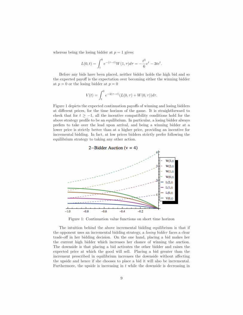
Consider an auction with 2 symmetric bidders with values and arrival ratesgiven by v = 4 and λ = 1, and let T = −1. We would like to construct anequilibrium in which bidders make only the minimal bid necessary to hold thecurrent high bid, whenever they arrive.

Formally, we consider a strategy profile in which a losing bidder bids p + 1when p ∈ {0, 1, 2, 3} and restrains from bidding when p ≥ 4. At the same time,a winning bidder restrains from increasing the current (proxy) price if she getsthe chance to do so.

Let W (p, t) and L(p, t) denote the expected payoffs of a winning bidder (thebidder holding the current high bid) and the losing bidder respectively at timet when current price is p, along the path of play when players adhere to thestrategies above. Note that we suppress the current high bid as this is uniquelydetermined by the price along the path of play.

Trivially, W (4, t) = 0 and L(p, t) = 0 for p ≥ 3. At p = 2 and p = 3 thewinning bidder gets a payoff of v−p if the other bidder does not arrive before theend of the auction and 0 otherwise. Therefore W (3, t) = et and W (2, t) = 2et.The expected value of being a losing bidder at L(2, t) is given by the expectationover the likelihood of arriving and becoming the winning bidder at p = 3,

L(2, t) =

∫ 0

t

e−(τ−t)W (3, τ)dτ = −tet

Similarly, L(1, t) = −2tet.The expected value of being a winning bidder at p = 1is equal to 4 if the other bidder does not arrive and is equal to the expectationof being the losing bidder at p = 2 if the other bidder does arrive.

W (1, t) =

∫ 0

t

e−(τ−t)L(2, τ)dτ + 3et =t2

2et + 3et

Being the winning bidder at p = 0:

W (0, t) =

∫ 0

t

e−(τ−t)L(1, τ)dτ + 4et = t2et + 4et

8

whereas being the losing bidder at p = 1 gives:

L(0, t) =

∫ 0

t

e−(τ−t)W (1, τ)dτ = − t3

6et − 3tet.

Before any bids have been placed, neither bidder holds the high bid and sothe expected payoff is the expectation over becoming either the winning bidderat p = 0 or the losing bidder at p = 0

V (t) =

∫ 0

t

e−2(τ−t)(L(0, τ) +W (0, τ))dτ.

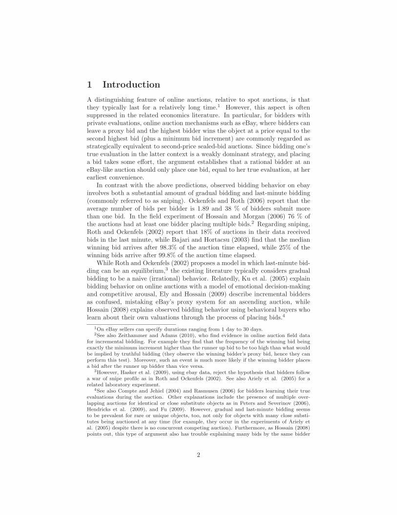
Figure 1 depicts the expected continuation payoffs of winning and losing biddersat different prices, for the time horizon of the game. It is straightforward tocheck that for t ≥ −1, all the incentive compatibility conditions hold for theabove strategy profile to be an equilibrium. In particular, a losing bidder alwaysprefers to take over the lead upon arrival, and being a winning bidder at alower price is strictly better than at a higher price, providing an incentive forincremental bidding. In fact, at low prices bidders strictly prefer following theequilibrium strategy to taking any other action.

Figure 1: Continuation value functions on short time horizon

The intuition behind the above incremental bidding equilibrium is that ifthe opponent uses an incremental bidding strategy, a losing bidder faces a cleartrade-off in her bidding decision. On the one hand, placing a bid makes herthe current high bidder which increases her chance of winning the auction.The downside is that placing a bid activates the other bidder and raises theexpected price at which the good will sell. Placing a bid greater than theincrement prescribed in equilibrium increases the downside without affectingthe upside and hence if she chooses to place a bid it will also be incremental.Furthermore, the upside is increasing in t while the downside is decreasing in

9

t. If an auction is short enough, it will support an incremental equilibrium inwhich bids are placed at every arrival by a losing bidder. This argument alsohints that in longer auctions equilibrium also requires periods of waiting (losingbidders passing on opportunities to place a bid and take over the lead), as theincentive to slow down the increase of the current price might become strongerthan the incentive to take over the lead. We discuss incremental equilibria withdelay in long auctions in Section 4.

We conclude this subsection by noting that in the above equilibrium, a bid-der’s expected payoff is V (0,−1) ≈ 1.45, and the expected revenue for the selleris (1− e−2)4− 2V (0,−1) ≈ 0.57. These expected payoffs are considerably morefavorable to the bidders than those in the benchmark equilibrium, in which theexpected payoffs are roughly 0.93 and 1.60 for the bidders and seller respectively.

3.2 Symmetric Markovian equilibria in short auctions

We now generalize the existence of equilibria with incremental bidding behavior.In particular, we characterize a class of equilibria in which bidding behavior onlydepends on the current price and whether the bidder is currently winning theobject.

Definition 1. A bidding sequence S = {b1, ..., bk} is an integer-valued set thatsatisfies 0 < b1 < ... < bk and bk ∈ {v − 1, v}. S is a completely gradual biddingsequence if S = {1, 2, . . . , v}.

Given a bidding sequence S, let us define for any price p ≤ v, lp as

lp,S = min{l : bl ≥ p}.

For the remainder of the paper, because the bidding sequence of interest willbe unambiguous, we abuse notation and write lp in reference to lp,S . This termis equal to p if p ∈ S and otherwise is the smallest element of S that is greaterthan p. With this we can formally introduce a class of Markovian strategiesthat we will study in this section.

Definition 2. A bidder bids incrementally over bidding sequence S = {b1, ..., bk}with no delays by bidding

1. blp+2 if p ≤ bk−2 and is the losing bidder,

2. v if bk−2 < p < v and is the losing bidder,

3. b1 if p = ∅,4. and otherwise refrains from bidding.

Furthermore a bidder bids completely gradually with no delays if S in theabove definition is the completely gradual bidding sequence.

10

Note that if players play according to the above strategy then the winningprice at any moment is equal to bl for some l, the current highest bid is bl+1,and the losing bidder upon arrival plans to place a bid of bl+2. This relativelysaddle way of prescribing strategies is necessary to induce players to place bidsalong a general bidding sequence, instead of deviating to bidding more graduallythan what the sequence prescribes. As we saw in the example in the previoussubsection, for the most gradual bidding sequence strategies can be defined ina simpler way: whenever price is p, a losing bidder when gets the chance placesa bid of p+1 (and if that was not enough to take over the bid then p+2, etc.).

Theorem 1. In an auction with n symmetric bidders, for any bidding sequenceS = {b1, . . . , bk} with bk = v, there exists a t∗ < 0 such that if T ≥ t∗ the auctionhas an equilibrium in which bidders follow the incremental bidding strategy withno delays over S.

Proof. The following proof is for the two bidder case where we can show thatincremental equilibria exist iff T ≥ − 1

λ . The proof for n bidders is conceptuallythe same but notationally more demanding, and it is given in the Appendix. LetW (p, t) and L(p, t) denote the expected continuation value of the winning andlosing bidder respectively at time t and current price p, conditional on biddersusing an incremental bidding strategy over S = {b1, ..., bk}. Additionally wedefine V (t) as the continuation value of the bidders at time t when no bids havebeen placed. Note that the continuation value can be expressed as a functionof b and t because of the Markovian assumption. We construct the expectedcontinuation values recursively, with L(bk, t) = 0 and W (bk, t) = (v − bk−1)e

λt

and for 0 < l < k,

L(bk−l, t) =

∫ 0

t

λe−λ(τ−t)W (bk−l+1, τ)dτ

W (bk−l, t) =

∫ 0

t

λe−λ(τ−t)L(bk−l+1, τ)dτ + (v − bk−l)eλt

The following incentive conditions on the continuation value functions are suf-ficient to show that an incremental bidding strategy is a best response:

L(bk−l, t) ≥ L(bk−l+1, t) (1)

W (bk−l+1, t) ≥ L(bk−l, t). (2)

The first condition ensures that incremental bids are weakly better than higherbids; higher bids weakly reduce the expected continuation value from becoming alosing bidder without affecting the expected continuation value from remainingthe winning bidder until the end of the auction. Note that this also impliesthat winning bidders will weakly prefer to not adjust their initial bid uponsubsequent arrival. The second inequality implies that making an incrementalbid is always weakly preferred to remaining a losing bidder. Note that the firstset of inequalities are trivially satisfied since for any realization of arrivals, the

11

losing bidder at time t at a highest bid of bk−l gets a weakly better payout thana losing bidder at time t at a highest bid of bk−l+1. We will now prove thatthe second set of inequalities hold with an inductive proof. Note the followingexpressions for the value functions:

W (bk, t) = 0

W (bk−1, t) = eλt(v − bk−2)

L(bk−1, t) = 0

L(bk−2, t) = −λteλt(v − bk−2)

Clearly W (bk, t) ≥ L(bk−l, t) and W (bk−1, t) ≥ L(bk−2, t) for all t ≥ −1/λ. Wenow prove the inductive step; if W (bk−l, t) ≥ L(bk−l−1, t) for all t ≥ −1/λ thenW (bk−l−2, t) ≥ L(bk−l−3, t) for all t ≥ −1/λ.

L(bk−l−3, t) =

∫ 0

t

λe−λ(τ−t)W (bk−l−2, τ)dτ

= −λteλt(v − bk−l−2) +

0∫t

λe−λ(τ−t)

0∫τ

λe−λ(s−τ)L(bk−l−1, s)dsdτ

≤ eλt(v − bk−l−2) +

0∫t

λe−λ(τ−t)

0∫τ

λe−λ(s−τ)W (bk−l, s)dsdτ

= W (bk−l−2, t),

where the inequality follows from our assumption that W (bk, t) ≥ L(bk−1, t)in addition to the fact that t ≥ −1/λ. This then proves the second set ofinequalities for all l. At the beginning of the auction both bidders are activeuntil the first bid is placed, hence the continuation values at B = 0 must betreated separately. The expected continuation value at B = 0 is given by,

L(∅, t) =

∫ 0

t

λe−2λ(τ−t)(W (0, τ) + L(0, τ))dτ

To prove that W (0, t) ≥ L(∅, t) for t ≥ −1/λ, consider a modified game withprice initialized at −1 and a modified bidding sequence for this game: S ={0, b1, . . . , bK}. Let L(p, t) and W (p, t) be the corresponding continuation valuefunctions at price p and time t in the modified game. Note that the recursiveargument used above implies that

L(−1, t) < W (0, t).

Furthermore note that W (0, t) = W (0, t) for all t. However L(∅, t) ≤ L(−1, t)for all t since for every realization of arrivals from a highest bid of 0 at timet, the realized payoff of the losing player in the modified game is weakly larger

12

than in the original game.11 This then allows us to conclude that

L(∅, t) < W (0, t)

as desired.This implies that it is always suboptimal for a losing bidder to pass on biddingopportunities. The way strategies are constructed then trivially implies thatneither underbidding (placing a bid below what is prescribed by the strategyprofile) or overbidding (placing a bid above the prescribed one) cannot be strictlyprofitable deviations.

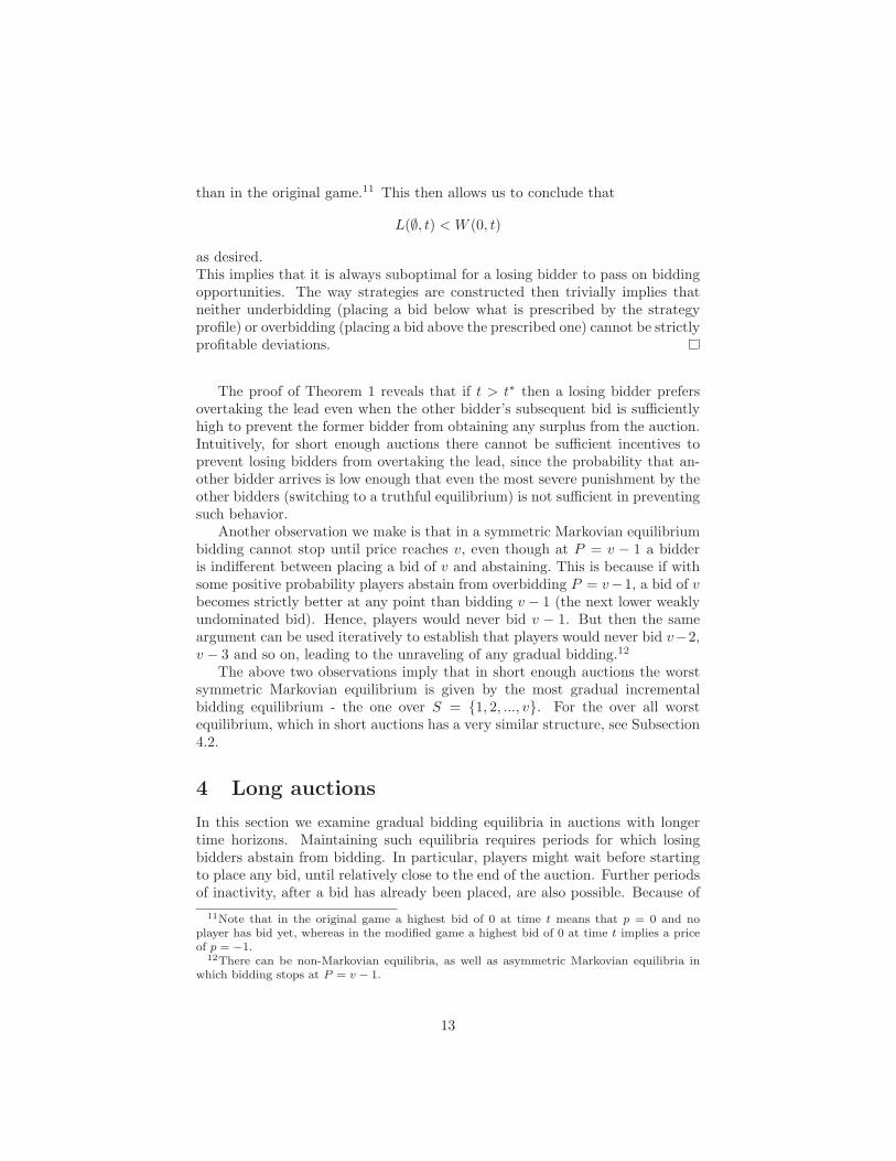
The proof of Theorem 1 reveals that if t > t∗ then a losing bidder prefersovertaking the lead even when the other bidder’s subsequent bid is sufficientlyhigh to prevent the former bidder from obtaining any surplus from the auction.Intuitively, for short enough auctions there cannot be sufficient incentives toprevent losing bidders from overtaking the lead, since the probability that an-other bidder arrives is low enough that even the most severe punishment by theother bidders (switching to a truthful equilibrium) is not sufficient in preventingsuch behavior.

Another observation we make is that in a symmetric Markovian equilibriumbidding cannot stop until price reaches v, even though at P = v − 1 a bidderis indifferent between placing a bid of v and abstaining. This is because if withsome positive probability players abstain from overbidding P = v−1, a bid of vbecomes strictly better at any point than bidding v − 1 (the next lower weaklyundominated bid). Hence, players would never bid v − 1. But then the sameargument can be used iteratively to establish that players would never bid v−2,v − 3 and so on, leading to the unraveling of any gradual bidding.12

The above two observations imply that in short enough auctions the worstsymmetric Markovian equilibrium is given by the most gradual incrementalbidding equilibrium - the one over S = {1, 2, ..., v}. For the over all worstequilibrium, which in short auctions has a very similar structure, see Subsection4.2.

4 Long auctions

In this section we examine gradual bidding equilibria in auctions with longertime horizons. Maintaining such equilibria requires periods for which losingbidders abstain from bidding. In particular, players might wait before startingto place any bid, until relatively close to the end of the auction. Further periodsof inactivity, after a bid has already been placed, are also possible. Because of

11Note that in the original game a highest bid of 0 at time t means that p = 0 and noplayer has bid yet, whereas in the modified game a highest bid of 0 at time t implies a priceof p = −1.

12There can be non-Markovian equilibria, as well as asymmetric Markovian equilibria inwhich bidding stops at P = v − 1.

13

this, no matter how long the auction is, the expected revenue of the seller inthese equilibria can be very small relative to v.

In Subsection 4.1 we provide an example of a gradual bidding equilibriumwith waiting. In long auctions it becomes considerably easier to construct grad-ual bidding equilibria using non-Markovian strategies, so in Subsection 4.2 wepropose a class of such equilibria, for any valuation and any number of bidders,that includes the over all worst equilibrium for the seller. In Subsection 4.3 wepropose a similar Markovian strategy profile that we show constitutes an equi-librium if the number of bidders is large enough. As the 2-bidder example inSubsection 4.1 shows, large number of bidders is not a necessary condition forthe existence of gradual bidding Markovian equilibria, but for a small number ofplayers it is difficult to provide a general recipe for constructing such equilibria.

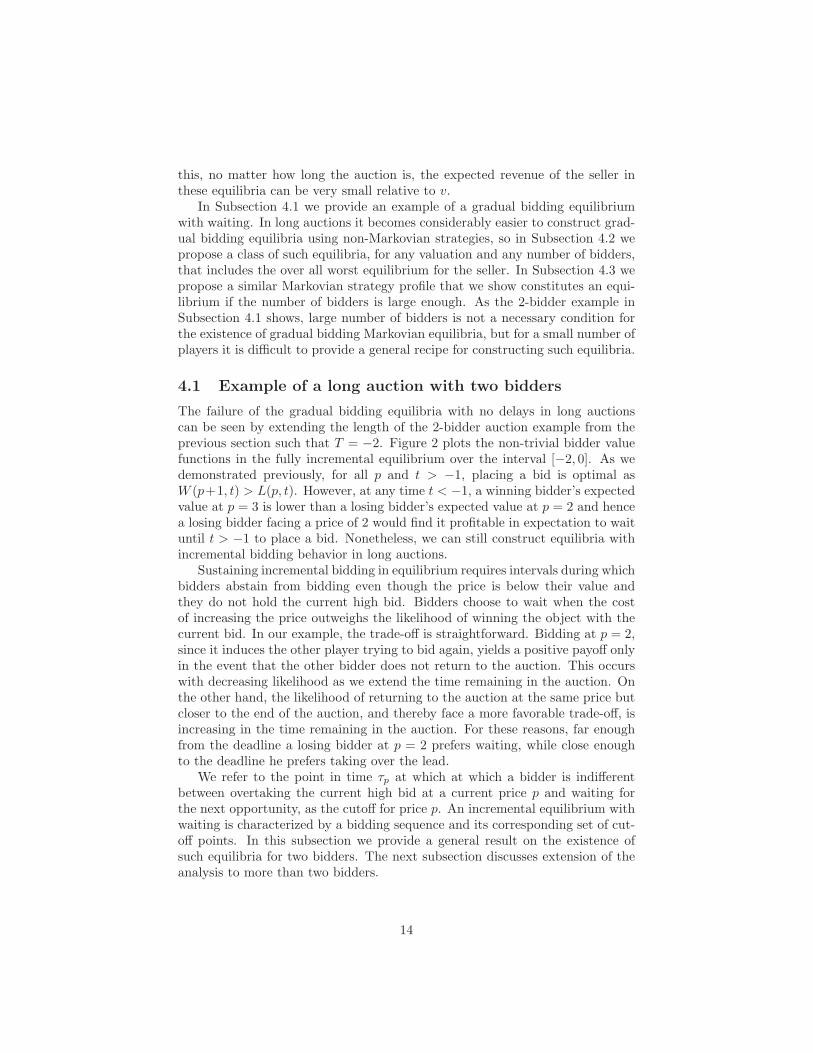
4.1 Example of a long auction with two bidders

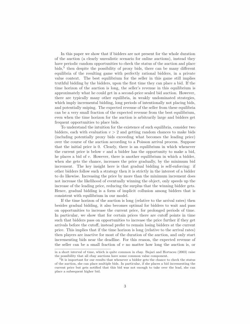
The failure of the gradual bidding equilibria with no delays in long auctionscan be seen by extending the length of the 2-bidder auction example from theprevious section such that T = −2. Figure 2 plots the non-trivial bidder valuefunctions in the fully incremental equilibrium over the interval [−2, 0]. As wedemonstrated previously, for all p and t > −1, placing a bid is optimal asW (p+1, t) > L(p, t). However, at any time t < −1, a winning bidder’s expectedvalue at p = 3 is lower than a losing bidder’s expected value at p = 2 and hencea losing bidder facing a price of 2 would find it profitable in expectation to waituntil t > −1 to place a bid. Nonetheless, we can still construct equilibria withincremental bidding behavior in long auctions.

Sustaining incremental bidding in equilibrium requires intervals during whichbidders abstain from bidding even though the price is below their value andthey do not hold the current high bid. Bidders choose to wait when the costof increasing the price outweighs the likelihood of winning the object with thecurrent bid. In our example, the trade-off is straightforward. Bidding at p = 2,since it induces the other player trying to bid again, yields a positive payoff onlyin the event that the other bidder does not return to the auction. This occurswith decreasing likelihood as we extend the time remaining in the auction. Onthe other hand, the likelihood of returning to the auction at the same price butcloser to the end of the auction, and thereby face a more favorable trade-off, isincreasing in the time remaining in the auction. For these reasons, far enoughfrom the deadline a losing bidder at p = 2 prefers waiting, while close enoughto the deadline he prefers taking over the lead.

We refer to the point in time τp at which at which a bidder is indifferentbetween overtaking the current high bid at a current price p and waiting forthe next opportunity, as the cutoff for price p. An incremental equilibrium withwaiting is characterized by a bidding sequence and its corresponding set of cut-off points. In this subsection we provide a general result on the existence ofsuch equilibria for two bidders. The next subsection discusses extension of theanalysis to more than two bidders.

14

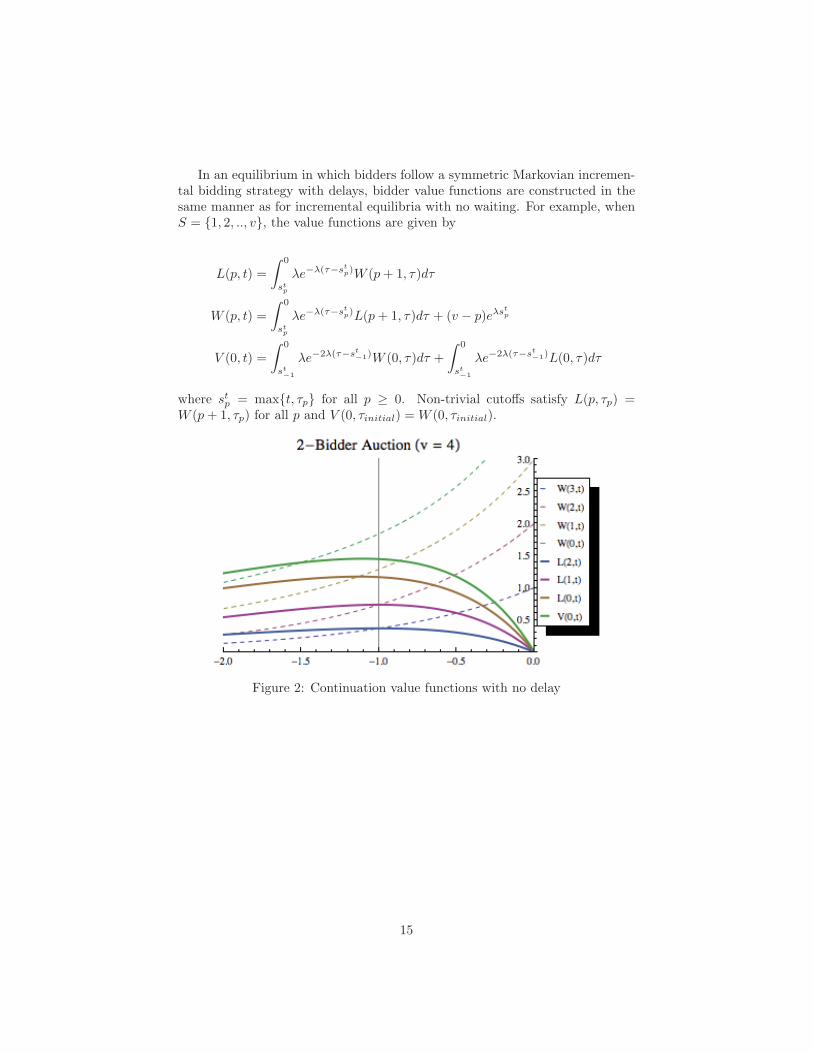
In an equilibrium in which bidders follow a symmetric Markovian incremen-tal bidding strategy with delays, bidder value functions are constructed in thesame manner as for incremental equilibria with no waiting. For example, whenS = {1, 2, .., v}, the value functions are given by

L(p, t) =

∫ 0

stp

λe−λ(τ−stp)W (p+ 1, τ)dτ

W (p, t) =

∫ 0

stp

λe−λ(τ−stp)L(p+ 1, τ)dτ + (v − p)eλstp

V (0, t) =

∫ 0

st−1

λe−2λ(τ−st−1)W (0, τ)dτ +

∫ 0

st−1

λe−2λ(τ−st−1)L(0, τ)dτ

where stp = max{t, τp} for all p ≥ 0. Non-trivial cutoffs satisfy L(p, τp) =W (p+ 1, τp) for all p and V (0, τinitial) = W (0, τinitial).

Figure 2: Continuation value functions with no delay

15

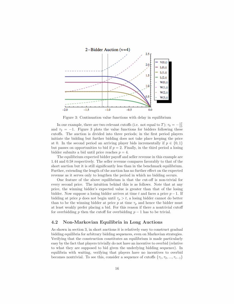
Figure 3: Continuation value functions with delay in equilibrium

In our example, there are two relevant cutoffs (i.e. not equal to T ); τ0 = − 1715

and τ2 = −1. Figure 3 plots the value functions for bidders following thesecutoffs. The auction is divided into three periods; in the first period playersinitiate the bidding but further bidding does not take place keeping the priceat 0. In the second period an arriving player bids incrementally if p ∈ {0, 1}but passes on opportunities to bid if p = 2. Finally, in the third period a losingbidder submits a bid until price reaches p = 4.

The equilibrium expected bidder payoff and seller revenue in this example are1.44 and 0.58 respectively. The seller revenue compares favorably to that of theshort auction but it is still significantly less than in the benchmark equilibrium.Further, extending the length of the auction has no further effect on the expectedrevenue as it serves only to lengthen the period in which no bidding occurs.

One feature of the above equilibrium is that the cut-off is non-trivial forevery second price. The intuition behind this is as follows. Note that at anyprice, the winning bidder’s expected value is greater than that of the losingbidder. Now suppose a losing bidder arrives at time t and faces a price p− 1. Ifbidding at price p does not begin until τp > t, a losing bidder cannot do betterthan to be the winning bidder at price p at time τp and hence the bidder mustat least weakly prefer placing a bid. For this reason if there a nontrivial cutofffor overbidding p then the cutoff for overbidding p− 1 has to be trivial.

4.2 Non-Markovian Equilibria in Long Auctions

As shown in section 3, in short auctions it is relatively easy to construct gradualbidding equilibria for arbitrary bidding sequences, even on Markovian strategies.Verifying that the construction constitutes an equilibrium is made particularlyeasy by the fact that players trivially do not have an incentive to overbid (relativeto what they are supposed to bid given the underlying bidding sequence). Inequilibria with waiting, verifying that players have no incentives to overbidbecomes nontrivial. To see this, consider a sequence of cutoffs {τ1, τ2, ..., τv−1}

16

and a strategy profile according to which a losing bidder bids incrementallywhenever price is p and t < τp, otherwise pass on the bidding opportunity.Suppose that τp for some p is a nontrivial cutoff. If a losing bidder i arrives att < τp when price is p− 2 then the above implies that the bidder faces a trade-off between placing a highest bid of p, as prescribed by the completely gradualbidding sequence, versus placing a bid of p + 1. On the one hand, the latteris better because it implies that if the other player gets a bidding opportunitybetween t and τp then she will bid p but refrain from further bidding. Thisensures that at time τp bidder i remains the winning bidder. The downsideof bidding p + 1 versus p is that the former implies that if the next arrival byanother player is after τp then she will not stop bidding at p, and takes overthe highest bid anyway, but at a higher price than what would have resulted ifi stuck to bidding gradually.

In this subsection we avoid this complication by considering a class of non-Markovian equilibria in which players restrain from overbidding because thelatter triggers a continuation equilibrium in which bidders switch to truthfulstrategies (placing a bid of v whenever possible), which is the most severe pun-ishment possible in equilibrium. In particular, we focus on equilibria that yieldthe worst payoffs among equilibria in which bidding is along a particular bid-ding sequence S, by maximally delaying the period of refraining from placing aparticular bid along the bidding sequence. We will consider Markovian gradualbidding equilibria in long auctions in the next subsection.

4.2.1 General Bidding Sequences

In order to define gradual bidding equilibria with periods of inactivity, we needto extend our definition of bidding sequences.

Definition 3. Let S = {b1, . . . , bk} be a bidding sequence. A strategy profile isan incremental bidding strategy profile with delay over bidding sequence S andcutoff sequence CS = {t∅, t0, . . . , tk−2} if on the equilibrium path,

1. no bidding occurs when t < tlp+2,

2. players bid blp+2 if t ≥ tlp+2 and lp ≤ k − 2,

3. players bid v if v > lp > k − 2,

4. and players bid b1 if p = ∅ and t ≥ t∅.

Note that the definition above only characterizes bidding behavior on theequilibrium path. We leave the strategies off the equilibrium path of play un-restricted in the definition and show that there exist equilibria whose outcomepath follows the definition above.

17

Theorem 2. Let S = {b1, . . . , bk}. Then there exists a cutoff sequence CS

such that there exists an equilibrium that is an incremental bidding strategyprofile with delay over S and CS. Moreover, among cutoff sequences whichcan constitute an equilibrium with the cutoff sentence, there is a maximal one{t∅, t0, . . . , tk−2}, in the sense that ti ≥ ti for any i ∈ {∅, 0, 1, ..., k−2} and cutoffsentence {t∅, t0, . . . , tk−2} that can constitute an equilibrium with the same cutoffsequence.

We will refer to the equilibrium in the second part of the statement as themaximally delayed equilibrium with the given bidding sequence. The construc-tion of such an equilibrium is quite intuitive. We use reversion to the truthfulequilibrium as punishment to deter deviations off the equilibrium path. Notehowever that such punishment is not useful for times very close to the deadlineof the auction. Thus we have a series of cutoff times for which players at a givenprice do not place bids before the cutoff due to the threat of reversion to thetruthful equilibrium but after which the player bids incrementally. We presentthe formal arguments in the following proof.

Proof. We proceed in a recursive manner. Denote by Wn(p, t) and Ln(p, t)the value functions for the winning and losing bidders in an n player auction atprice p and time t conditional on all players playing according to the incrementalbidding strategy over S with no delay. Define tln as the maximal time at whichreversion to the truthful equilibrium is no longer sufficient to deter bidding ata price of bl:

eλ(n−1)tln(v − bl+1) = Ln(bl, tln).

Then define tk−2 = tk−2n and also

W (bk−2, t) =

{Wn(bk−2, t) if t ≥ tk−2

Wn(bk−2, tk−2) if t < tk−2

L(bk−2, t) =

{Ln(bk−2, t) if t ≥ tk−2

Ln(bk−2, tk−2) if t < tk−2.

With this defined, we now define the other cutoffs recursively. Suppose thattl+1 and W (bl+1, t) and L(bl+1, t) have been defined. Then let

W (bl, t) = eλ(n−1)t(v − bl) +

0∫t

λe−λ(n−1)(τ−t)(n− 1)L(bl+1, τ)dτ,

L(bl, t) =

0∫t

λe−λ(n−1)(τ−t) (W (bl+1, τ) + (n− 2)L(bl+1, τ)) dτ.

We can now define tl implicitly as:

L(bl, tl) = eλ(n−1)tl(v − bl+1).

18

Then we define

W (bl, t) =

{W (bl, t) if t ≥ tl

W (bl, t) if t < tl,

L(bl, t) =

{L(bl, t) if t ≥ tl

L(bl, t) if t < tl.

Iterating we can construct all of the relevant cutoffs t0, t1, . . . , tk−2 and all ofthe relevant continuation value functions. In a similar manner we construct thecutoff t∅. Given W (0, t), L(0, t), we define

L(∅, t) =0∫

t

λe−λn(τ−t) (W (0, τ) + (n− 1)L(0, τ)) dτ.

Then define t∅ asL(∅, t∅) = eλ(n−1)t∅v.

Furthermore we define the continuation value when no player has bid as:

L(∅, t) ={L(∅, t) if t ≥ t∅

L(∅, t∅) if t < t∅.

With all of these cutoffs defined, we are now ready to define the candidatestrategy profile. Define first the set H:

H = {h ∈ H : (p, t) ∈ h and p /∈ S or p > bl, t < tl for some l}.

In words this is the set of histories where either some player has been revealedto have bid some amount not in the bid sequence or to have placed a bidabove bl before time tl. It turns out that these histories form the histories offthe equilibrium path of play in the following candidate strategy profile. Thecandidate strategy profile is defined as follows.

1. If p = ∅, bid b1 if and only if t ≥ t∅.

2. If h /∈ H and �h = (p, t) with p �= ∅, then bid blp+2 if and only if t ≥ tlp

and the bidder is losing.

3. If h ∈ H, bid v.

4. Otherwise refrain from bidding.

First note that any element of h ∈ H is not on the outcome path of playaccording to this strategy profile. With this observation, it is easy to check thateach player has incentives to play according to the strategy specified above.

19

The strategies constructed above have the special feature that on the equilib-rium path, bidding takes the form of incremental bidding with delays accordingto the cutoff sequence t∅, . . . , tk−2. Such behavior is optimal due to the threatof reversion to the truthful equilibrium when players deviate to a history offthe equilibrium path of play by bidding when the strategy prescribes them topostpone their bids until a later time.

4.2.2 Special Bidding Sequences

For a general bidding sequence, the maximally delayed equilibrium constructedabove can be complicated, with multiple subsequent waiting periods belongingto different prices. Here we provide a sufficient condition on the bidding sequencefor the maximally delayed equilibrium to have a simple structure, for any numberof bidders, in which there are at most two effective cutoff times, and all waitingis frontloaded in the auction. This simple structure allows us to iterativelycharacterize cutoffs and equilibrium continuation values. We also show that thesame result holds for any bidding sequence when the number of bidders is large.

Let S = {b1, . . . , bk} be a bidding sequence. We call a bidding sequenceregular if the following assumption holds:

v − bk−l

v − bk−l−1≤ v − bk−l−1

v − bk−l−2.

A sufficient condition for the above to hold is if the increments are weakly de-creasing and thus for example, the completely gradual bidding sequence satisfiesthe above property.

Theorem 3. Let S = {b1, . . . , bk} be a regular bidding sequence. Then thecutoff sequence belonging to a maximally delayed equilibrium satisfies that tl isdecreasing in l for l ∈ {0, 1, ..., k − 2}.

Note that the statement implies that there can only be either one or twoeffective cutoffs along the equilibrium path: either t∅ and t0, or only t∅. This isbecause players only overbid a winning price of 0 after t0, which is weakly laterthan all cutoffs belonging to higher prices, hence bidding from this time on isgradual with no waiting, just like at a short auction.

To prove the theorem, we define the cutoff tl as the latest time at whichreversion to a truthful equilibrium is not sufficient to deter a losing bidder frombidding:

eλ(n−1)tl(v − bl+1) = Ln(bl, tl)

where Ln(bl, t) is defined as the continuation value of a losing bidder at time tconditional on all players in the future following a gradual bidding strategy overthe bid sequence S.

To establish that tl is indeed decreasing in l, we first show that when theregularity condition holds, the continuation payoff of a losing bidder at any timet decreases by a relatively greater factor due to a price increase from bl−1 to bl

20

than the value of the object at those respective prices. This then implies thatif tl−1 is such that

eλ(n−1)tl−1

(v − bl) = Ln(bl−1, tl−1),

it must be thateλ(n−1)tl−1

(v − bl+1) > Ln(bl, tl−1),

which means that tl < tl−1. Note however that the monotonicity claim doesnot extend to the cutoff t∅. The reason is that Ln(∅, t) has a slightly differentfunctional form than Ln(bl, t) for l ≥ 0 (since if no one bid yet then there are nlosing bidders potentially wanting to place bids, while in any other case thereare only n−1 losing bidders). Therefore the structure of equilibria may be suchthat there are two effective cutoffs at both t∅ and t0 along the equilibrium path.The proof in its full detail is in Section A.4 in the Appendix.

Similarly the next result establishes that for arbitrary bidding sequences,when the number of bidders is large enough, maximally delayed equilibria againhave the property that once a bid is placed, cutoffs are monotonically decreasingin price. This means that when the number of bidders is large, any biddingsequence admits a structure of equilibrium that is qualitatively similar to thatof a regular bidding sequence. Therefore as we have shown for regular biddingsequences, the equilibrium path of play in maximally delayed equilibria for anyarbitrary sequence with a large number of bidders is such that all of the delayoccurs at the beginning of the auction at the prices of ∅ and 0 (or only at ∅, ift0 ≤ t∅).

Theorem 4. Let S = {b1, ..., bk} be a bidding sequence. Then for sufficientlylarge n, the cutoff sequence belonging to a maximally delayed equilibrium satisfies

t∅ > t0 > t1 > · · · > tk−2 = −1/λ.

The proof of this theorem exploits the properties of the functions Ln(bl, t)and Wn(bl, t), defined as the continuation of a losing and winning bidder con-ditional on all players playing according to a gradual bidding strategy profilewith no delays. We again define tln for a choice of n to be the time at which

eλ(n−1)tln(v − bl+1) = Ln(bl, tln).

Given a collection of cutoffs (at each n) for a price of bl, we argue that the nor-malized continuation value of a losing bidder at a price equal to the next highest

bid, e−λ(n−1)tlnLn(bl−1, tln), must become arbitrarily large as n approaches ∞.

This then means that for n sufficiently large,

Ln(bl−1, tln) > eλ(n−1)tln(v − bl).

Again using the fact that Ln(bl−1, t) is decreasing, we conclude that tl−1n > tln.

The proof is relegated to Section A.4 in the Appendix.

21

4.2.3 Worst Equilibrium

History dependent strategies allow the construction of equilibria that furtherreduce the seller’s expected revenue beyond the equilibria constructed in theprevious section. In this section we characterize the seller-revenue minimizingequilibria in 2-bidder auctions. Strategies in the seller revenue-minimizing equi-librium take the following form: bidders pass on all bidding opportunities priorto t∗ < 0 after which bidders engage in incremental bidding without delay overS = {1, 2, ...v− 3, v− 2, v− 1}. When the price reaches v− 2, any losing bidderarrives and places a bid of v. However, when the price reaches v− 1, no furtherbidding occurs. Any deviation in this stage is punished by reverting to a truth-ful equilibrium, which is the most severe punishment a defector can face as itimplies that any subsequent arrival by the other bidder reduces the deviator’spayoff to 0.

We begin by noting that the threat of punishment allows the final bid tobe v − 1 without causing unravelling; the threat of punishment makes a bidderindifferent between bidding v − 2 and v − 1. Further, if t∗ is greater than thefinal cutoff in the equilibrium without punishment then placing any bid strictlydominates waiting. In particular this means placing a bid of v dominates waitingand hence the threat of punishment cannot induce a bidder to wait.

In a symmetric value auction with 2 bidders, let W (p, t, v) and L(p, t, v)denote the expected payoffs of winning and losing bidders respectively at timet, price p, and symmetric valuation v, conditional on bidders following an in-cremental bidding strategy over S = {1, 2, ...v − 3, v − 2, v − 1} and at leastone bidder having placed a bid. Also let V (0, t, v) be the expected payoff ofthe bidder at time t when nobody has placed a bid. The cutoff t∗v is the pointat which reversion to truthful bidding no longer provides sufficient incentivesfor a bidder to refrain from bidding. Therefore, at t∗v a bidder is indifferentbetween triggering truthful bidding, for an expected payoff of vet

∗v , and waiting,

which yields an expected payoff of V (0, t∗v, v). We begin by showing that t∗v isincreasing in v. Suppose t∗v satisfies

vet∗v =

∫ 0

t∗v

e−2(τ−t∗v) (W (0, τ, v) + L(0, τ, v)) dτ.

Consider the following function in t∗:

vet∗ −

∫ 0

t∗e−2(τ−t∗) (W (0, τ, v) + L(0, τ, v)) dτ.

First note that the derivative of the above function with respect to t∗ is

vet∗ −

∫ 0

t∗2e−2(τ−t∗) (W (0, τ, v) + L(0, τ, v)) dτ +W (0, t∗, v) + L(0, t∗, v)

> W (0, t∗, v) + L(0, t∗, v)−∫ 0

t∗e−2(τ−t∗) (W (0, τ, v) + L(0, τ, v)) dτ > 0

22

for all t∗ > t∗v by the definition of t∗v and the fact that L(0, t∗, v) > 0. Therefore,

vet∗>

∫ 0

t∗e−2(τ−t∗) (W (0, τ, v) + L(0, τ, v)) dτ

for all t∗ > t∗v. Note also that∫ 0

t∗ve−2(τ−t∗v) (W (0, τ, v + 1) + L(0, τ, v + 1)) dτ∫ 0

t∗ve−2(τ−t∗v) (W (0, τ, v) + L(0, τ, v)) dτ

>v + 1

v.

Therefore

(v + 1)et∗v <

∫ 0

t∗v

e−2(τ−t∗v) (W (0, τ, v + 1) + L(0, τ, v + 1)) dτ.

The above observations then imply that t∗v must be increasing in v.It now remains only to demonstrate that bidding is maximally delayed, which

is a straightforward point. The sum of the expected continuation values ofthe two bidders in an auction of length t∗ with arbitrary equilibrium biddingsequence R is bounded above by that of the same auction with equilibriumbidding sequence S. Hence, if a bidder is indifferent at time t between triggeringpunishment and waiting given the bidding sequence S, the bidder must weaklyprefer triggering the punishment for any other bidding sequence T . Therefore,the proposed strategies form the seller minimizing equilibrium.

The cutoff value t∗v is increasing in v, as at a higher v players can be inducedto wait longer, through trigger strategies. Numerical calculations show that t∗v isincreasing in v fast enough so that the expected number of bids and therefore theseller’s expected revenue is decreasing in v (larger t∗v implies a smaller expectednumber of arrivals during the period when players are actively bidding, and thisoutweights the effect that bidding can potentially reach higher prices if v is largerand a lot of arrival events occur towards the end). Hence these computationssuggest that the ratio of the seller’s expected revenue to the bidder’s value vgoes to zero as v grows large.

4.3 Markovian Equilibria in Long Auctions

Constructing Markovian equilibria in long auctions is complicated, for the rea-sons spelled out at the beginning of Subsection 4.2. However, in this Subsectionwe show that for a large number of bidders, the construction of equilibriumstrategies simplifies considerably, for any bidding sequence.

4.3.1 The Completely Gradual Bidding Sequence

The completely gradual bidding sequence has a convenient feature that we donot need to check incentives to underbid since the latter is infeasible by defi-nition. Therefore we begin our analysis with this bidding sequence and latershow that the constructions for the completely gradual bidding sequence can bemodified to accommodate general bidding sequences.

23

Definition 4. A strategy profile is a Markovian completely gradual biddingstrategy profile with delays over the cutoff sequence C = {t∅, t0, . . . , tv−2, tv−1}if she places a bid of p+1 at a price of p and time t if and only if she is a losingbidder and t ≥ tp. Otherwise she refrains from bidding.

Note first that these strategies do indeed restrict play at histories that occuroff the equilibrium path of play as well as those on the equilibrium path. Thisadditional restriction differentiates these strategies from those of the previoussection where behavior off the equilibrium path was left flexible. For this reason,the equilibrium constructions of Subsection 4.2 exhibit more delay in biddingbecause players can use the harshest punishment available, namely reversionto the truthful equilibrium, to deter any deviations off the equilibrium path.In this section, such use of punishment is prohibited as the class of strategiesstudied here are more restrictive. The next result states that for the completelygradual bidding sequence, if the number of bidders is large enough, there existsan equilibrium that is a Markovian completely gradual bidding strategy profilewith delays over some cutoff sequence.

Theorem 5. There exists an n∗ such that for all n > n∗, there exists a cutoffsequence C = {t∅, t0, . . . , tv−2, tv−1} such that the strategy profile in which allplayers bid completely gradually with delays over C is an equilibrium.

To prove this result, we first let the cutoffs be the furthest time away fromthe deadline at which he would prefer to submit a bid of l+2 and thus increasingthe price to l + 1 rather than delaying any bidding, conditional on all biddersin the future following a strategy profile of complete gradual bidding with nodelays. These cutoffs can be defined uniquely for each n. Moreover, for large n,we show that this cutoff sequence is monotonic so that

tv−1 < tv−2 < · · · < t0 < t∅.

Having established monotonicity of cutoffs, it is easy to define continuationvalues consistent with completely gradual bidding over the cutoff sequence de-fined. Because the cutoff sequence is monotonic, after any time t > tl at anyprice at least l, play according to the defined strategy profile follows completegradual bidding with no delays. Then with the aid of some useful properties ofthese continuation value functions that we establish in the proof, one can checkincentive compatibility of the strategies following a technique similar to the oneused in the section on short auctions.

Proof. We denote by Wn(p, t) and Ln(p, t) respectively the continuation valuefunctions of a winning and losing bidder in an n player auction at a price oftime t conditional on all bidders following a incremental bidding strategy withno delays over the bid sequence S = {1, . . . , v}. First define the cutoffs tln asthe time at at which

Wn(l + 1, tln) = Ln(l, tln).

24

We define a similar cutoff denoted t∅n when p = ∅. Note first that such a timetln, if it exists, must be strictly negative for all l ≤ v − 2, since at time 0,Wn(l + 1, 0) > 0 = Ln(l, 0). Furthermore in Section A.5 Lemma 5, we showthat there exists some n∗ such that for all n > n∗ > 2,

tv−2n < tv−3

n < · · · t0n < t∅n.

We assume that n∗ > 2 for later parts of the proof. Let n > n∗ and settl = tln for all l = ∅, 0, . . . , v − 2 and also let tv−1 = −∞. We now show thatcompletely gradual bidding over the cutoff sequence C = {t∅, t0, . . . , tv−2, tv−1}constitutes an equilibrium. The continuation value functions for the winningand losing bidders for the above strategies can be defined easily as follows dueto the monotonic pattern of cutoffs:

W (l, t) =

{Wn(l, t) if t > tl

Wn(l, tl) if t ≤ tl.(3)

L(l, t) =

{Ln(l, t) if t > tl

Ln(l, tl) if t ≤ tl.(4)

If instead the cutoffs above did not display the monotonic pattern exhibited here,then the continuation values will have to be redefined in a more complicatedmanner. The reason is that the monotonic pattern of cutoffs implies that aftertime tl given a price of l, play according to the above strategies constitutescompletely gradual bidding without delays. Therefore after time tl, at a priceof tl the continuation values of a losing and winning bidder are exactly thesame as the continuation values of the same bidding sequence computed for ashort auction. Before we check the incentives of all bidders to follow the strategyprofile described, we demonstrate first that the value functions W and L exhibitthe following properties:

1. W (l, t) is weakly increasing in t.

2. W (l, t) > W (l+1, t) and L(l, t) ≥ L(l+1, t) for all t and all l = 0, . . . , k−1.

Let us prove the first claim. Consider W (l, t). The claim is obvious for l = v.Then note that for all t ≥ tl−1

n > tln > tl+1n , W (l, t) ≥ L(l − 1, t) ≥ L(l + 1, t).

This means that W (l, t) is increasing for all t ≥ tl−1n due to Lemma 3 in the

Appendix. Furthermore it is constant for all t ≤ tln. Thus it remains to checkthe monotonicity of W (l, t) for all t ∈ (tln, t

l−1n ).

W (bl+1, t) > W (bl+2, t) > L(bl+1, t)

for all t > tl+1n . Then for all t > tln,

W (l, t) > W (l + 1, t) > W (l + 2, t) > L(l + 1, t).

Then this means that W (l, t) is increasing for all t > tln again due to Lemma 3in the Appendix. Thus we have proved point 1. Given the above, monotonicity

25

in the price of the value functions for the winning bidders is almost trivial.Consider the functions W (l, t) and W (l+1, t). From Lemma 2, we know for allt ≥ tln,

W (l, t) = Wn(l, t) > Wn(l + 1, t) = W (l + 1, t).

Furthermore for all t < tln,

W (l, t) = Wn(l, tln) > Wn(l + 1, tln) = W (l + 1, tln) ≥ W (l + 1, t).

Now consider the value functions of the losing bidders, L(l, t) and L(l + 1, t).First note that

L(l, t) = Ln(l, t) > Ln(l + 1, t) = L(l + 1, t)

for all t ≥ tln by Lemma 2. Then

L(l, t) = L(l, tln) = W (l + 1, tln) ≥ W (l + 1, t) > W (l + 2, t) > L(l + 1, t).

for all t ∈ [tl+1n , tln). Then note that for all t < tl+1

n ,

L(l, t) = L(l, tl+1n ) > L(l + 1, tl+1

n ) = L(l + 1, t).

With these properties, it is easy to check the incentives of all players. Supposefirst that the price is p �= ∅, t < tp, and the bidder is a losing bidder. Placing abid of p′ > p+ 1 generates a payoff of

0∫max{tp+1,t}

λe−λ(n−1)(τ−max{tp+1n ,t})(n− 1)L(p′, τ)dτ,

whereas not bidding generates a payoff of

L(p, t) = L(p, tp)

= W (p+ 1, tp)

≥ W (p+ 1, t)

=

0∫max{tp+1,t}

λe−λ(n−1)(τ−max{tp+1n ,t})(n− 1)L(p+ 2, τ)dτ.

where the inequality follows from property 1 above. Since property 2 aboveimplies that L(p + 2, τ) ≥ L(p′, τ) for all p′ ≥ p + 2, we have shown that itis suboptimal to bid any amount greater than p′. It is also suboptimal to bidp+ 1. To see this note that the payoff from bidding p+ 1 is

0∫max{tp+1,t}

λe−λ(n−1)(τ−max{tp+1,t}) (W (p+ 1, τ) + (n− 2)L(p+ 1, τ)) dτ

26

since any losing bidder at a price p believes with probability one that the highestbid is p+1. Note that the above expression is exactly equal to Ln(p,max{t, tp+1}).Furthermore not bidding generates a payoff of L(p, tp) = Ln(p, tp). Note that

∂

∂tLn(p, t) = λ(Ln(p, t)−Wn(p+ 1, t)) + λ(n− 2)(Ln(p, t)− Ln(p+ 1, t)) > 0

for all t ≤ tp which implies that Ln(p, t) < Ln(p, tp). This then proves that it issuboptimal to place any bid at such a time. Consider a winning bidder at sucha time. Given that players do not place any bids before time tp, it is trivialto check that placing any further bids is suboptimal. Suppose that the currenthighest bid is b. Then placing a bid of b′ > b gives a payoff of

eλ(n−1)tp(v − p) +

0∫tp

λe−λ(n−1)(τ−tp)(n− 1)L(b′, τ)dτ

which is less than the payoff obtained from not placing any bid:

eλ(n−1)tp(v − p) +

0∫tp

λe−λ(n−1)(τ−tp)(n− 1)L(b, τ)dτ.

Finally let us consider the incentives to bid gradually when the price is p andt ≥ tp. A winning bidder again clearly does not want to place any bids sincethis only increases the price in the future without affecting the probability ofwinning the object. Formally, if the current high bid is b, bidding some amountb′ > b generates a payoff of

eλ(n−1)tp(v − p) +

0∫tp

λe−λ(n−1)(τ−tp)(n− 1)L(b′, τ)dτ

which is clearly less than the expected payoff of not placing any bids:

eλ(n−1)tp(v − p) +

0∫tp

λe−λ(n−1)(τ−tp)(n− 1)L(b, τ)dτ.

Now consider a losing bidder. Such a bidder, by not placing a bid, obtains apayoff of L(p, t) = Ln(p, t) whereas placing a bid of p + 2 generates a bid ofW (p + 1, t) = Wn(p + 1, t). We know from Corollary 1 in the Appendix thatW (p + 1, t) ≥ L(p, t) for all t ≥ tp. Thus it is suboptimal to not place a bid.Placing a bid of b′ > p+2 is also suboptimal since the payoff of such a strategyis less than W (p+1, t). Placing a bid of p+1 followed by no other bids generatesa payoff of Ln(p, t) which is again less than W (p+ 1, t). Thus it is optimal forsuch a losing bidder to place a bid of p+2, which is exactly equivalent to placinga bid of p+ 1 followed by a bid of p+ 2 in the same arrival. This concludes theproof.

27

One of the important features of the equilibrium construction above is themonotonicity of the cutoffs: tv−2 < tv−3 < · · · < t0 < t∅. In fact this pattern ofcutoffs implies that on the equilibrium path of the strategies constructed in theproof, there is a period of inactivity in which no player bids until t∅ after whichplayers bid completely gradually with no delays.

4.3.2 General Bidding Sequences

In this subsection, we extend the construction of the previous subsection toaccommodate general bidding sequences. A modification is necessary to deterunderbidding since players can potentially place a bid less than the next bid inthe bidding sequence to slow down the rate of price increase.

Definition 5. Let S = {b1, . . . , bk} be a bidding sequence. Then a bidder bidsincrementally over S and CS = {t∅, t0, . . . , tk−2} if upon arrival at a price p andtime t,

1. a bidder places a bid of blp+2 if p ≤ bk−2 and t ≥ tp,

2. bids v if bk−2 < p < v,

3. bids b1 if t ≥ t∅ and p = ∅,4. and otherwise, refrains from bidding.

Note that the only difference in the bidding strategies defined above fromthat of the bidding strategies for the completely gradual bidding sequence is thaton the equilibrium path, players place a bid of bl+2 immediately when the priceis bl and the cutoff time has passed. This is exactly equivalent to the equilibriumoutcome behavior in the completely gradual bidding equilibrium with delays.This is necessary here to prevent underbidding when the price is p = ∅, whereasin the completely gradual bidding sequence, such issues are non-existent sinceany price p = 0, 1, 2, . . . , v arises on the equilibrium path.

Then with the definition above, we obtain a similar existence theorem for ageneral bidding sequence for sufficiently large n.

Theorem 6. Let S = {b1, . . . , bk} be a bidding sequence. Then exists some n∗

such that for all n > n∗, there exists a cutoff sequence CS = {t∅, t0, . . . , tk−2}such that incremental bidding over S and CS forms an equilibrium.

The only part of the proof that differs from the proof of the analogoustheorem for the completely gradual bidding sequence is that players may havean incentive to underbid. The proof that underbidding is suboptimal is similarto the proof illustrated in the proof of Theorem 1. Thus we leave the details forthe Appendix.

28

5 Extension: Time-dependent arrival rates

In the previous version of the paper we considered several extensions of ourframework, such as asymmetric arrival rates, asymmetric valuations, and asym-metric information regarding valuations. For all these environments it is possibleto create gradual bidding equilibria similar to those featured in the current pa-per. Here we only consider relaxing the assumption of constant arrival ratesthroughout the auction’s time horizon.

First, note that multiplying all arrival rates by a constant α > 0 is equivalentto rescaling time by 1

α . In particular, if the original game has an incrementalbidding strategy equilibrium over bidding sentence {b1, ..., bk} and cutoff sen-tence {t1, ..., tk} then the game where arrival rates are multiplied by α has anincremental bidding strategy equilibrium over bidding sentence {b1, ..., bk} andcutoff sentence { 1

α t1, ...,1α tk}. Furthermore, expected payoffs with time horizon

T in the original game are the same as with time horizon Tα in the game with

the rescaled arrival rates. In particular, if T ≤ t1 then increasing arrival ratesand keeping the time horizon the same does not change equilibrium expectedpayoffs: it only shifts all cutoffs to the right, in an inversely proportional man-ner. Intuitively, if bidders get frequent opportunities to place bids, it makesthem postpone bidding at different price levels until later, in a way that exactlyoffsets the effect of increasing the arrival rates.

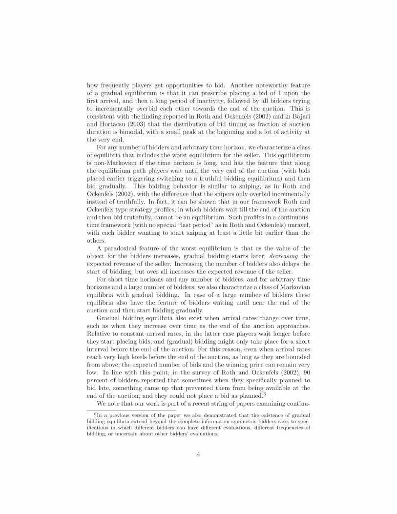
Figure 4: A time-dependent arrival rate

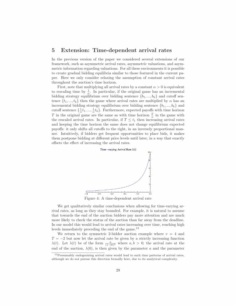
We get qualitatively similar conclusions when allowing for time-varying ar-rival rates, as long as they stay bounded. For example, it is natural to assumethat towards the end of the auction bidders pay more attention and are muchmore likely to check the status of the auction than far away from the deadline.In our model this would lead to arrival rates increasing over time, reaching highlevels immediately preceding the end of the game.13

We return to the symmetric 2-bidder auction example where v = 4 andT = −2 but now let the arrival rate be given by a strictly increasing functionλ(t). Let λ(t) be of the form a

(1−bt)2 where a, b > 0; the arrival rate at the

end of the auction, λ(0), is then given by the parameter a and the parameter

13Presumably endogenizing arrival rates would lead to such time patterns of arrival rates,although we do not pursue this direction formally here, due to its analytical complexity.

29

b determines how steeply arrival rates increase at the end of the auction. The

average arrival rate over the auction is given by λ =∫ 0

−2a

(1−bt)2 dt. We choose

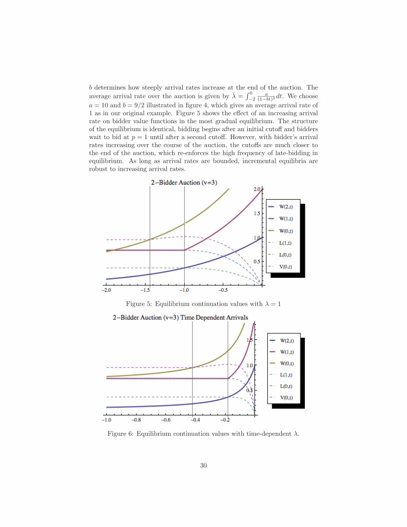
a = 10 and b = 9/2 illustrated in figure 4, which gives an average arrival rate of1 as in our original example. Figure 5 shows the effect of an increasing arrivalrate on bidder value functions in the most gradual equilibrium. The structureof the equilibrium is identical, bidding begins after an initial cutoff and bidderswait to bid at p = 1 until after a second cutoff. However, with bidder’s arrivalrates increasing over the course of the auction, the cutoffs are much closer tothe end of the auction, which re-enforces the high frequency of late-bidding inequilibrium. As long as arrival rates are bounded, incremental equilibria arerobust to increasing arrival rates.

Figure 5: Equilibrium continuation values with λ = 1

Figure 6: Equilibrium continuation values with time-dependent λ.

30

6 Conclusion

This paper shows that on online auctions like ebay where bidders can leaveproxy bids, if bidders get random chances to place bids then many differentequilibria arise in weakly undominated strategies. Bidders can implicitly colludeby bidding gradually or by waiting to place bids, in a self-enforcing manner,slowing down the increase of leading price. These features of our model areconsistent with the empirical observations that both gradual bidding and snipingare common bidder behaviors on ebay.

Our investigation suggests that given a fixed set of bidders, running anascending auction with a long time horizon (long enough that bidders cannotcontinuously participate) has the potential to affect the revenue of the seller veryadversely, even when proxy bidding is possible, relative to running a promptauction. Hence, introducing a time element can only be beneficial if it takestime for potential bidders to find out about the auction.14 It is an open questionwhat mechanism guarantees the highest possible revenue for the seller in suchenvironments. In order to prevent implicit collusive equilibria, sellers mightwant to set high reservation prices and/or minimum bid increments. Theymight also want to allow each bidder to submit at most one bid over the courseof an auction, although in practice this might be difficult to enforce, giventhat the same person can have multiple online identities. We leave the formalinvestigation of these issues to future research.

14In a recent paper, Fuchs and Skrzypacz (2010) considers the arrival of new buyers overtime, but in a dynamic bargaining context in which the seller cannot commit to a mechanism.Another difference compared to our setting is that in their model once a buyer arrives, she iscontinuously present until the end of negotiations.

31

A Appendix

A.1 Proof of Claim 1

Proof of Claim 1: A strategy that at a given history calls for placing a bid ofb > v is conditionally weakly dominated by a strategy that at the same historycalls for placing a bid of v if v > P and abstaining from bidding otherwise,and specifies the same behavioral strategy as the original strategy at any otherhistory.

Take now any history satisfying the requirements in part (ii) of the state-ment. For any possible B given the history, a strategy that specifies abstainingfrom bidding at time t gives at most B(1− etλi) expected payoff, while a strat-egy that calls for i incrementally bidding at this history until either i becomesa winner or P = v yields at least BetΣj �=iλj . Since t ≥ t∗i , the latter expectedpayoff is weakly larger. Moreover, if there is such a B strictly smaller than vthen there exists a strategy profile of the other bidders that is consistent withthe given history and for which a strategy that calls for i incrementally biddingat this history until either i becomes a winner or P = v yields a strictly higherpayoff (conditional on the history) than a strategy that calls for abstaining. Inparticular, any strategy profile of the others consistent with the given informa-tion set and B < v, and also satisfying that other bidders do not increase theirbids at any history after t implies a strict payoff difference.

The above conclude that (i) and (ii) are necessary for a strategy to be con-ditionally weakly undominated.

Assume now that a strategy si of player i satisfies properties (i) and (ii),but it is conditionally weakly dominated by strategy s′i. Then there has to be atime-t history h for some t ≤ 0 at which (i/a) si and s′i specify different biddingbehavior; (i/b) if at h either player i is the winning bidder or no one bid yet,then the final bid bidder i places at t, conditionally on h, differs between si ands′i; (iii) conditional on the history the expected payoff induced by s′i is weaklylarger than the one induced by si for any strategy profile of the other biddersconsistent with the given history, and there exists a strategy profile of the otherbidders consistent with the given history for which the inequality is strict. Thelast condition implies that there is a strategy profile of the others consistentwith the history such that B < v.

First, note that s′i has to satisfy condition (i) in the claim too, otherwise therewould be a history and a strategy profile of the others such that conditional onthe history s′i yields a negative payoff to i, contradicting that it conditionallyweakly dominates si.

Second, we note that if at h either no one placed a bid yet or player i is thecurrent winning bidder, and conditional on h both si and s′i specify bidding upB at t to either v or v − 1, then si yields at least as much payoff as s′i, for anystrategy profile of the other bidders. This is because other bidders can only findout whether B is higher than v − 1 if another bidder placed a bid of at leastv (otherwise they have to play the same way against si and s′i, as they cannottell them apart). But in the latter case player i’s payoff becomes 0 whether

32

playing si or s′i, contradicting that the latter conditionally weakly dominatesthe former.

Consider now the case that at h either player i is the winning bidder orno one bid yet, and conditional on h, si and s′i both specify placing a bid butspecify different final bids at t, bi and b′i, such that at least one of them is strictlyless than v − 1. If bi > b′i then si yields a higher expected payoff against s′i ifthe other players from time t on play a strategy prescribing placing a bid ofmin(bi, v− 1) if winning price is below that and otherwise abstaining. If bi < b′ithen si yields a higher expected payoff against s′i if the others follow a strategythat after t prescribes bidding bi + 1 if price is below that, and if that was notenough to take over the lead then bidding v at the same arrival opportunity,otherwise abstaining from placing further bids for the remainder of the auction.In both cases, si cannot be conditionally weakly dominated by s′i.

Consider now the case that at h player i is the winning bidder with B < v−1,and conditional on h si prescribes increasing the bid to b > B, while s′i prescribesnot bidding at this history. Then si yields a higher expected payoff than s′i ifthe strategies of other bidders call for placing a bid of B + 1 upon first arrivaland abstaining otherwise.

Consider now the case that at h player i is the winning bidder with B <v − 1, and conditional on h si prescribes not placing a bid, while s′i prescribesincreasing the bid to b > B. Then si yields a higher expected payoff against s′iif the others follow a strategy that after t prescribes bidding B + 1 if price isbelow that, and if that was not enough to take over the lead then bidding v atthe same arrival opportunity, otherwise abstaining from placing further bids forthe remainder of the auction.

Consider now that at h player i is a losing bidder, and strategy si calls forabstaining, while strategy s′i calls for placing a bid. Since si satisfies property(ii) in the claim, t < t∗i . But then the definition of t∗i implies that for a strategyprofile of the others that is consistent with h, implies B < v at the history, andspecifies a continuation strategy of abstaining from bidding in the future if i doesnot place a bid at t, but a continuation strategy of bidding v the first possibleoccasion in case i does place a bid at t, si gives a strictly higher expected payoffthan s′i. This contradicts that s

′i weakly dominates si.

Consider now that at h player i is a losing bidder, and si calls for placing abid, while s′i calls for abstaining. Consider then a strategy profile of the othersthat is consistent with the history, implies B < v at h, and specifies continuationstrategies for the others to bid v upon first arrival if player i does not place a bidat t, and abstain in the future if player i places a bid. If t ≥ t∗i , the assumptionthat si satisfies property (ii) in the claim (therefore keeps on bidding untiltakes over winning at price B) implies that her expected payoff induced by siconditional on h is v − B, while her conditional expected payoff induced by s′iis lower than that, contradicting that s′i conditionally dominates si. Considernow t < t∗i . Since satisfies property (ii) in the claim, it yields an expectedpayoff of at least (v −B)(1− et

∗i λi), while s′i yields less than (v −B)etΣj �=iλj <

(v − B)et∗i Σj �=iλj = (v − B)(1 − et

∗i λi). This contradicts that s′i conditionally

dominates si.

33

The only cases remain to be considered are when h is such that a bid isalready placed, player i is losing, and si and s′i call for placing different bids ath. Denote these bids b and b′.

Consider first b > b′. If at history h someone already placed a bid thenconsider any strategy profile for the others that is consistent with h, impliesB = b− 1, and after t prescribe continuation strategies for the other bidders toplace a bid of v if at t player i either did not place any bids or the first bid of idid not make her the winning bidder, and otherwise abstain from placing a bidafter t. Then si yields a strictly higher expected payoff conditional on h thans′i, contradicting that the latter conditionally weakly dominates the former.

Consider now b < b′. Consider a strategy profile of the other bidders thatis consistent with h, implies B = v − 1, and prescribes abstaining after t ifat t someone places a bid that does not change the identity of the winner butchanges the winning price to b, and otherwise placing a bid of v upon firstarrival. Note that t < t∗i then the assumption that si satisfies property (i) inthe claim implies that si yields a (sure) payoff of 1, while s′i yields an expectedpayoff of etΣj �=iλj < 1. If t ≥ t∗i then si yields an expected payoff of at least1− et

∗i λi , while s′i yields an expected payoff of etΣj �=iλj < et

∗i Σj �=iλj = 1− et

∗i λi .

Both cases contradict that s′i conditionally weakly dominates si. �

A.2 Proof of Theorem 1 (n-bidders)

Bidder value functions are given by,

W (bk, t) =

∫ 0

t

λe−(m+1)λ(τ−t)(n− 1)L(bk+1, τ)dτ + (v − bk)e(n−1)λt

L(bk, t) =

∫ 0

t

λe−(m+1)λ(τ−t) (W (bk+1, τ) + (n− 2)L(bk+1, τ)) dτ

We construct t∗ as follows,

W (bk, t)− L(bk−1, t)

=

∫ 0

t

λe−(m+1)λ(τ−t) ((m+ 1)L(bk+1, τ)−mL(bk, τ)−W (bk, τ)) dτ + (v − bk−1)e(m+1)λt

> −∫ 0

t

λe−(m+1)λ(τ−t) (m(L(bk, τ)− L(bk+1, τ)) +W (bk, τ)) dτ + (v − bk−1)e(m+1)λt

=(e(m+1)λt − 1) (m(bk+1 − bk) + (v − bk−1))

m+ 1+ (v − bk−1)e

(m+1)λt

≥ 0

34

for all t,

tk =log(

m(bk+1−bk)+(v−bk−1+1)m(bk+1−bk)+2(v−bk−1+1)+m(v−bk−1+1)

)m+ 1

≤ t < 0

Let t∗ = maxk tk and we have W (bk, t) − L(bk−1, t) > 0 for t > t∗. Astraightforward induction argument proves that the other incentive constraints,L(bk−1, t)− L(bk, t) > 0 also hold for t > t∗.

A.3 Calculation of Value Functions with n bidders forShort Auctions

In this section, we will show that the value functions for an n-bidder auctionalong the bid sequence S = {b1, . . . , bk} with no delays take the following form:15

W (bk−l, t) = eλ(n−1)tl−1∑j=0

(−λt)j

j!

((n− 1)j

n+

(−1)j(n− 1)

n

)(v − bk−l+j) (5)

L(bk−l, t) = eλ(n−1)tl−1∑j=0

(−λt)j

j!

((n− 1)j

n+

(−1)j+1

n

)(v − bk−l+j) (6)

L(∅, t) = eλ(n−1)tk−1∑j=0

(−1)j+1

⎛⎝ ∞∑l=j+1

(λt)l

l!

⎞⎠ (n− 1)j(v − bj). (7)

These expressions are quite easily obtained when n = 2. The analysis forn = 2 is quite easy due to the fact that, given gradual bidding with no delays overS, the outcome path of winning bidders is simply an alternation between thetwo players. However when n > 2 there are many more possible permutationsof bidding outcomes on the equilibrium path. Thus the derivation of the aboveexpressions is more complicated.

These closed form expressions of the value functions will be useful in ouranalysis of long auctions, as they remain valid in those auction for times closeenough to the deadline. In particular, for a large number of players they enableus to show monotonicity of cutoffs in prices, which greatly simplify verifyingthat the strategy profiles we consider constitute equilibria.

A.3.1 A Simple Markov Chain

To derive the expressions above, we first analyze a simple Markov chain whosestate space is the set of players {1, . . . , n}. The transition matrix for this finite

15Here we assume the convention that 00 = 1 and that 0! = 1.

35

state Markov chain is as follows:

M ≡

⎛⎜⎜⎜⎝0 1

n−11

n−1 · · · 1n−1

1n−1 0 1

n−1 · · · 1n−1

......

......

...1

n−11

n−11

n−1 · · · 0

⎞⎟⎟⎟⎠ .

The interpretation for this Markov chain is the following. The state variables ∈ {1, . . . , n} represents the identity of the winner at each stage. The processthen transitions to a new winner s′ ∈ {1, . . . , n}−s in the next period accordingto the above transition matrix. According to the transition matrix, each of thebidders who is not a winner has equal probability of becoming a winner in thenext stage. Note that this transition matrix is important for our analysis, sincethis transition matrix compounded with an appropriate Poisson arrival processrepresents the equilibrium outcome path of strategies in gradual bidding withno delays.

We first analyze the matrixM j which represents the conditional probabilitiesof each individual being a winner at the end of j stages. Let E be a matrixwhose elements consist of only ones. Then

M j =1

(n− 1)j(E − I)j

=1

(n− 1)j

j∑l=0

(jl

)(−1)lEj−l

= (−1)j1

(n− 1)jI +

1

(n− 1)j

j−1∑l=0

(jl

)(−1)lnj−l−1E

= (−1)j1

(n− 1)jI +

1

(n− 1)jE

n

j−1∑l=0

(jl

)(if − 1)lnj−l

=1

(n− 1)j

((−1)jI +

((n− 1)j + (−1)j+1)

nE

).

Then if a bidder is a winner, the probability that he is a winner at the end of jstages is equal to dj = M j

1,1 = M j2,2 = · · · = M j

n,n which is

dj =1

n+

(−1)j

n(n− 1)j−1.

Similarly if he is a loser, the probability that he becomes a winner at the endof j stages is equal to

fj =1

n+

(−1)j+1

n(n− 1)j

which is equal to the elements of M j not on the diagonal.

36

A.3.2 Value functions

Then we can use the result above to arrive at the following formula for the valuefunctions of a winning and losing bidder at price bk−l conditional on all playersfollowing an incremental bidding strategy with no delays over the bid sequenceS:

W (bk−l, t) = eλ(n−1)tl−1∑j=0

(−λt)j

j!(n− 1)jdj(v − bk−l+j)

= eλ(n−1)tl−1∑j=0

(−λt)j

j!

((n− 1)j + (−1)j(n− 1)

n

)(v − bk−l+j)

L(bk−l, t) = eλ(n−1)tl−1∑j=0

(−λt)j

j!(n− 1)jfj(v − bk−l+j)

= eλ(n−1)tl−1∑j=0

(−λt)j

j!

((n− 1)j + (−1)j+1

n

)(v − bk−l+j)

When k = l, the above is

W (0, t) = eλ(n−1)tk−1∑j=0

(−λt)j

j!

((n− 1)j + (−1)j(n− 1)

n

)(v − bj)

L(0, t) = eλ(n−1)tk−1∑j=0

(−λt)j

j!

((n− 1)j + (−1)j+1

n

)(v − bj)

Then we can calculate L(∅, t).

L(∅, t) =0∫

t

λe−λn(τ−t)(W (0, τ) + (n− 1)L(0, τ))dτ

= eλnt0∫

t

λe−λτe−λ(n−1)τ (W (0, τ) + (n− 1)L(0, τ))dτ

= eλnt0∫

t

λe−λτ

⎛⎝k−1∑j=0

(−λτ)j

j!(n− 1)j(v − bj)

⎞⎠ dτ

= eλ(n−1)tk−1∑j=0

(n− 1)j(v − bj)eλt

0∫t

λe−λτ (−λτ)j

j!dτ.

We can simplify the above expression further with the following lemma.

37

Lemma 1.

hj(t) = eλt0∫

t

λe−λτ (−λτ)j

j!dτ = (−1)j

((j∑

l=0

(λt)l

l!

)− eλt

)

= (−1)j+1∞∑

l=j+1

(λt)l

l!

Proof. The proof is shown by induction on j and integration by parts. Theclaim is obvious for j = 0. Now suppose that the claim holds for j. Then

0∫t

λe−λτ (−λτ)j+1

(j + 1)!dτ =

(−λt)j+1

(j + 1)!e−λt −

0∫t

(−λτ)j

j!λe−λτdτ

=(−λt)j+1

(j + 1)!e−λt + (−1)j+1

(e−λt

(j∑

l=0

(λt)l

l!

)− 1

)

= (−1)j+1

(e−λt

(j+1∑l=0

(λt)l

l!

)− 1

).

This concludes the proof.

This then gives us the expressions for the value functions given by equations(5), (6), and (7) at the beginning of this section.

A.3.3 Properties of the Value Functions

In this section, we prove some basic properties of the value functions derived inthe previous section. These basic properties will be used throughout the paper.

Lemma 2. Ln(bk−l, t) > Ln(bk−l+1, t) for all t and all l ≥ 2. Also, Wn(bk−l, t) >Wn(bk−l+1, t) for all t.

The proof is obvious from the expressions in (5) and (6), hence omitted.Next we use this lemma to prove some basic properties of the value functions.

Lemma 3. The following hold:

1. e−λ(n−1)tLn(bk−l, t) is strictly decreasing for all t < 0 for all l ≥ 2.

2. ∂∂tW

n(bk−l, t) > 0 when Wn(bk−l, t) ≥ Ln(bk−l+1, t).

3. ∂∂t (W

n(bk−l+1, t)− Ln(bk−l, t)) > 0 when Wn(bk−l+1, t) ≥ Ln(bk−l, t).

4. e−λ(n−1)tLn(∅, t) is strictly decreasing for all t < 0.

38

5. ∂∂t (W

n(0, t)− Ln(∅, t)) > 0 when Wn(0, t) ≥ Ln(∅, t).Proof. Consider the first statement.

e−λ(n−1)tLn(bk−l, t) =

l−1∑j=0

(−λ(n− 1)t)j

j!fj(v − bk−l+j)

The derivative of the function with respect to t gives:

−λ(n− 1)

l−1∑j=1

(−λ(n− 1)t)j−1

(j − 1)!fj(v − bk−l+j) < 0.

Now consider the second statement.

Wn(bk−l+1, t) = eλ(n−1)t(v − bk−l+1) +

0∫t

λe−λ(n−1)(τ−t)(n− 1)Ln(bk−l+2, τ)dτ.

Due to the fundamental theorem of calculus, the derivative of the above expres-sion is

λ(n− 1)(Wn(bk−l+1, t)− Ln(bk−l+2, t)).

Note that the expression above is positive since

Wn(bk−l+1, t) ≥ Ln(bk−l, t) > Ln(bk−l+2, t).

We establish statement 3 with a similar argument.

Ln(bk−l, t) =

0∫t

λe−λ(n−1)(τ−t)(Wn(bk−l+1, τ) + (n− 2)Ln(bk−l+1, τ))dτ.

Again using the fundamental theorem of calculus, the derivative of the aboveexpression is

λ((n− 1)Ln(bk−l, t)−Wn(bk−l+1, t)− (n− 2)Ln(bk−l+1, t)).

Therefore

∂

∂t(Wn(bk−l+1, t)− Ln(bk−l, t)) = λ(n− 1)(Wn(bk−l+1, t)− Ln(bk−l, t))

+ λ(Wn(bk−l+1, t)− Ln(bk−l+2, t))

+ λ(n− 2)(Ln(bk−l+1, t)− Ln(bk−l+2, t)).

All of the terms above are positive, proving statement 3. Statement 4 is provedin the same manner as claim 1.

e−λ(n−1)tLn(∅, t) =k−1∑j=0

hj(t)(n− 1)j(v − bj)

39

Note that

∂

∂thj(t) = λ

(hj(t)− (−λt)j

j!

)= λ

((−1)j

((j∑

l=0

(λt)l

l!

)− eλt

)− (−λt)j

j!

)

= λ

⎛⎝(−1)j+1

⎛⎝ ∞∑l=j

(λt)l

l!

⎞⎠⎞⎠ < 0

for all t < 0. This then implies that e−λ(n−1)tLn(∅, t) is strictly decreasing in tfor all t < 0.

∂

∂tWn(0, t) = λ(n− 1)(Wn(0, t)− Ln(b1, t)).

Now consider the derivative of the value function Ln(∅, t).∂

∂tLn(∅, t) = λnLn(∅, t)− λWn(0, t)− λ(n− 1)Ln(0, t).

Thus

∂

∂t(Wn(0, t)− Ln(∅, t)) = λn(Wn(0, t)− Ln(∅, t))

+ λ(n− 1)(Ln(0, t)− Ln(b1, t)).

Note that all of the terms in the above expression are positive. This provesstatement 5.

An immediate corollary of lemma above is the following.

Corollary 1. Suppose Wn(bk−l+1, t∗) = Ln(bk−l, t

∗). Then Wn(bk−l+1, t) >Ln(bk−l, t) for all t > t∗ and Wn(bk−l+1, t) < Ln(bk−l, t) for all t < t∗. Simi-larly suppose Wn(0, t∗) = Ln(∅, t∗). Then Wn(0, t) > Ln(∅, t) for all t > t∗ andWn(0, t) < Ln(∅, t) for all t < t∗.

Proof. Suppose Wn(bk−l+1, t∗) = Ln(bk−1, t

∗). Then by the previous lemma,∂∂t (W

n(bk−l+1, t∗)−Ln(bk−l, t

∗)) > 0. This immediately implies thatWn(bk−l+1, t) >Ln(bk−l, t) for all t > t∗. This proves the first part of the claim. Now supposethat for some t′ < t∗,Wn(bk−l+1, t

′) ≥ Ln(bk−l, t′). Because ∂

∂t (Wn(bk−l+1, t

∗)−Ln(bk−l, t

∗)) > 0, there exists some ε > 0 such that Wn(bk−l+1, t) < Ln(bk−l, t)for all t ∈ (t∗ − ε, t∗). But then this implies that there exists some t′′ ∈ [t′, t∗)such that Wn(bk−l+1, t

′′) = Ln(bk−l, t′′). From what we already proved above,

this means that Wn(bk−l+1, t) > Ln(bk−l, t) for all t > t′′, which is a clear con-tradiction. This proves the claim. The claim for the value functions Wn(0, t)and Ln(∅, t) can be proved in exactly the same manner.

40

A.4 Non-Markovian Equilibria with Delays

A.4.1 Proof of Theorem 3

The key step in the proof is the following lemma.

Lemma 4. If S = {b1, . . . , bk} is regular, the continuation values for the losingbidders conditional on all bidders following the incremental bidding sequencewith no delays over S have the following property:

Ln(bk−l, t)

Ln(bk−l−1, t)≤ v − bk−l+1

v − bk−l.

Proof. First note the following continuation values:

Ln(bk−1, t) = 0

Ln(bk−2, t) = −λteλ(n−1)t(v − bk−1)

Ln(bk−3, t) = −λteλ(n−1)t(v − bk−2) +λ2t2

2eλ(n−1)t(n− 2)(v − bk−1).

Then it is easy to verify that

Ln(bk−1, t)

Ln(bk−2, t)≤ v − bk

v − bk−1,

Ln(bk−2, t)

Ln(bk−3, t)≤ v − bk−1

v − bk−2.

Now suppose that

Ln(bk−l+1, t)

Ln(bk−l, t)≤ v − bk−l+2

v − bk−l+1,

Ln(bk−l+2, t)

Ln(bk−l+1, t)≤ v − bk−l+3

v − bk−l+2.

Then we can write the value function for the losing bidder as:

Ln(bk−l, t)

v − bk−l+1= −λteλt(n−1) +

0∫t

λ(n− 2)e−λ(τ−t)(n−1)Ln(bk−l+1, τ)

v − bk−l+1dτ

+

0∫t

0∫τ

λ2e−λ(s−t)(n−1)(n− 1)Ln(bk−l+2, s)

v − bk−l+1dsdτ

≤ −λteλt(n−1) +

0∫t

λ(n− 2)e−λ(τ−t)(n−1)Ln(bk−l, τ)

v − bk−ldτ

+

0∫t

0∫τ

λ2e−λ(s−t)(n−1)(n− 1)Ln(bk−l+1, s)

v − bk−ldsdτ

=Ln(bk−l−1, t)

v − bk−l.

41

This proves the lemma.

Let us now define the cutoff tl in the following way.

eλ(n−1)tl(v − bl+1) = Ln(bl, tl).

Note that this does not have to be the time at which reversion to truthful biddingby all players is no longer sufficient to deter a losing bidder from bidding sincethe continuation value used in the definition is not necessarily equal to the actualcontinuation value. However, Lemma 4 together with Lemma 3 implies that tl

is decreasing in l for l ∈ {0, ..., k − 2}. This then implies that the continuationvalues of a losing bidder when price is bl are correct for the relevant range, thatis for times later than max

j∈{0,...,l}tj .

Then the above cutoff sequence is indeed the one belonging to a maximallydelayed equilibrium given bidding sequence S, hence in the latter tl is decreasingin l for l ∈ {1, ..., k − 2}. �

Given these cutoffs, we can then define the actual continuation values of thewinning and losing bidders in the same manner as in the proof of theorem 2.

W (bl, t) =

{Wn(bl, t) if t ≥ tl

Wn(bl, tl) if t < tl.

L(bl, t) =

{Ln(bl, t) if t ≥ tl

Ln(bl, tl if t < tl

for all l = 0, 1, . . . , v − 2. Continuation values at prices bk and bk−1 are definedas usual, W (bk, t), L(bk, t), L(bk−1, t) = 0 and W (bk−1, t) = Wn(bk−1, t) for allt. Clearly these definitions above rely on the fact that t0 ≥ t1 ≥ · · · ≥ tk−2.Furthermore we can define

L(∅, t) =0∫

t

λe−λn(τ−t) (W (0, τ) + (n− 1)L(0, τ)) dτ.

and finally t∅:L(∅, t∅) = eλ(n−1)t∅v.

Then define

L(∅, t) ={L(∅, t) if t ≥ t∅

L(∅, t∅) if t < t∅.

42

A.4.2 Proof of Theorem 4

In the proof below we use the expressions for value functions in short auctionsthat we calculated above, for continuation values towards the end of the game.

Let us define the following cutoffs tk−ln :

Ln(bk−l, tk−ln ) = (v − bk−l+1)e

λ(n−1)tk−ln .

Proof of Theorem 4: Consider the case in which l = 2.

L(bk−2, t) = eλ(n−1)t(−λt)(v − bk−1)

This then implies that tk−2n = −1/λ for all n. Consider now l = 3.

e−λ(n−1)tL(bk−3, t) = (−λt)(v − bk−2) +(−λt)2

2(n− 2)(v − bk−1)

Notice then that e−λ(n−1)tLn(bk−3, tk−2n ) > v − bk−2 for all n > 2. This means

that tk−3n > tk−2

n for all n > 2. Furthermore it is easy to conclude that tk−3n → 0

from the definition of tk−3n :

(−λtk−3n )(v − bk−2) +

(−λtk−3n )2

2(n− 2)(v − bk−1) = v − bk−2.

Given the fact that tk−3n → 0, we must have

n(−λtk−3n )2 → 2

v − bk−2

v − bk−1.

Now we induct based on the following inductive hypothesis:

1. lim infn→∞ nj−2(−λtk−jn )j−1 > 0,

2. tk−jn → 0,

3. and tk−2n < tk−3

n < · · · < tk−ln

for all 2 < j ≤ l and all n ≥ n∗. Clearly the above holds for l = 3 as we haveshown above. Suppose the above holds for some l. Consider the cutoff tk−l−1

n .First note that since lim infn→∞ nl−2(−λtk−l

n )l−1 > 0 and tk−ln → 0,

lim infn→∞n(−λtk−l

n ) = +∞.

Thereforelim inf

n→∞nl−1(−λtk−ln )l = +∞.

Observe the following expression:

e−λ(n−1)tk−ln L(bk−l−1, t

k−ln ) =

l∑j=0

(−λtk−ln )j

j!

((n− 1)j

n+

(−1)j+1

n

)(v − bk−l−1+j)

>(−λtk−l

n )l

l!

((n− 1)l

n+

(−1)l+1

n

)(v − bk−1)

→+∞.

43

This then immediately implies that for n sufficiently large, tk−l−1n > tln since

e−λ(n−1)tL(bk−l−1, t) is a decreasing function due to Lemma 3. This also impliesthat tk−l−1

n → 0. Now consider the following limit:

lim infn→∞nl−1(−λtk−l−1

n )l.

Suppose that the above is zero. Then it is easy to show that

lim infn→∞nj−1(−λtk−l−1

n )j = 0

for all j ≤ l which implies that

(v − bk−l) = lim infn→∞ e−λ(n−1)tk−l−1

n L(bk−l−1, tk−l−1n )

= lim infn→∞

l∑j=0

(−λtk−l−1n )j

j!

((n− 1)j

n+

(−1)j+1

n

)(v − bk−l−1+j)

=0,

a clear contradiction. Therefore we must have lim infn→∞ nl−1(−λtk−l−1n )l > 0.

Lastly, we examine the cutoff when p = ∅, when no players have bid. Define t∅nas the cutoff when

L(∅, t∅n) = veλ(n−1)t∅n .

Note that

e−λ(n−1)t0nL(∅, t0n) =k−1∑j=0

(−1)j+1

⎛⎝ ∞∑l=j+1

(λt0n)l

l!

⎞⎠ (n− 1)j(v − bj)

≥ (−1)k

( ∞∑l=k

(λt0n)l

l!

)(n− 1)k−1(v − bk−1).

Since lim infn→∞ nk−2(−t0n)k−1 > 0 and t0n → 0, using precisely the same argu-

ment used in the inductive step of the proof in the previous section, we musthave

lim infn→∞nk−1(−t0n)

k = +∞.

Then we know that

(−1)k

( ∞∑l=k

(λt0n)l

l!

)(n− 1)k−1(v − bk−1)

≥(n− 1)k−1(−λt0n)k

(1

k!+

λt0n(k + 1)!

)(v − bk−1)

The limit infimum of the last expression then goes to +∞ as n → ∞. Thus

lim infn→∞ e−λ(n−1)t0nL(∅, t0n) = +∞.

44

Thus we must have t∅n > t0n for n sufficiently large. In conclusion, we have shownthat for n sufficiently large,

−1/λ = tk−2n < tk−3

n < · · · < t0n < t∅n.

A.5 Markovian Equilibria with Delays for Large n

A.5.1 Monotonicity of Cutoffs

With the closed form expressions for the value functions given by equations (5),(6), and (7), we can also study how the structure of equilibria changes as wevary n. As in section A.4, we are particularly interested in the structure ofequilibria when the number of bidders is large relative to k, the number of bidsin a bid sequence. Let us study cutoffs tk−l

n where

Wn(bk−l+1, tk−ln ) = Ln(bk−l, t

k−ln )

where the value functions above represent the continuation values at time t inan auction with n bidders bidding incrementally over S = {b1, . . . , bk} with nodelays. To analyze these cutoffs, we use a similar method of proof used in theSection A.4 to study the following expressions for large values of n.

Wn(bk−l, t) = eλ(n−1)tl−1∑j=0

(−λt)j

j!

((n− 1)j

n+

(−1)j(n− 1)

n

)(v − bk−l+j)

Ln(bk−l, t) = eλ(n−1)tl−1∑j=0

(−λt)j

j!

((n− 1)j

n+

(−1)j+1

n

)(v − bk−l+j).

Lemma 5. Let S = {b1, . . . , bk} be a bid sequence. Then there exists some n∗

such thatt∅n > t0n > · · · > tk−2

n = −1/λ

for all n > n∗.

Proof. First we claim that cutoffs above ∅ are decreasing in price. We proceedby induction. Consider the case in which l = 2.

Wn(bk−1, tk−2n )− Ln(bk−2, t

k−2n ) = (v − bk−1)(1 + λtk−2

n )eλ(n−1)tk−2n

So tk−2n = −1/λ for all n. But then consider

(Wn(bk−2, tk−2n )− Ln(bk−3, t

k−2n ))e−λ(n−1)t1n

=(v − bk−2)(1 + λtk−2n )− (−λtk−2

n )2

2(n− 2)(v − bk−1)

<0

45

when n > 2. Thus for sufficiently large n, tk−2n < tk−3

n due to Corollary 1.Furthermore we can conclude that tk−3

n → 0 and that limn→∞ n(−λtk−3n )2 =

(v − bk−2)/(v − bk−1) > 0. Now we induct. Suppose that there exists some n∗

such that

1. lim infn→∞ nj−2(−λtk−jn )j−1 > 0,

2. lim supn→∞ nj−2(−λtk−jn )j−1 < ∞,

3. tk−jn → 0,

4. and tk−2n < tk−3

n < · · · < tk−ln

for all 2 < j ≤ l and all n ≥ n∗. Obviously, as we have already shown, all ofthe assumptions above hold for l = 3. Suppose the above hypotheses hold forl ≥ 3. Consider the cutoff tk−l−1

n . Then

lim infn→∞

nl−2(−λtk−ln )l−1

tln= lim inf

n→∞(−λntk−ln )l−2 = +∞.

Thuslim

n→∞−λntk−ln = +∞

which implieslim

n→∞nl−1(−λtk−ln )l = +∞.

Then consider the expression

e−λ(n−1)tk−ln(Wn(bk−l, t

k−ln )− Ln(bk−(l+1), t

k−ln )

)We first show that the above is negative for sufficiently large n. The aboveexpression is

l−1∑j=0

(−λtk−ln )j

j!

((n− 1)j

n+

(−1)j(n− 1)

n

)(v − bk−l+j)

−l∑

j=0

(−λtk−ln )j

j!

((n− 1)j

n+

(−1)j+1

n

)(v − bk−l+j−1)

The above is less than or equal to

v − bk−l +

l−1∑j=2

(−λtk−(j+1)n )j

j!

((n− 1)j

n+

(−1)j(n− 1)

n

)(v − bk−l+j)

− (−λtk−ln )l

l!

((n− 1)l

n+

(−1)l+1

n

)(v − bk−1)

for sufficiently large n. But by the inductive hypothesis the above goes to −∞as n → ∞. This then implies that for sufficiently large n,

Wn(bk−l, tk−ln )− Ln(bk−l−1, t

k−ln ) < 0.

46

Therefore tk−l−1n > tk−l

n for sufficiently large n due to Corollary 1. Now we needto prove the other statements used in the inductive hypothesis. Clearly sincetk−ln → 0, we must have tk−l−1

n → 0. Consider

lim infn→∞nl−1(−λtk−l−1

n )l.

Suppose that this expression is 0. Then

0 = lim infn→∞n

(l−1)2

l (−λtk−l−1n )l−1 ≥ lim inf

n→∞nl−2(−λtk−l−1n )l−1

Iterating we obtainlim inf

n→∞nj−1(−λtk−l−1n )j = 0

for all 1 ≤ j ≤ l. By definition

l−1∑j=0

(−λtk−l−1n )j

j!

((n− 1)j

n+

(−1)j(n− 1)

n

)(v − bk−l+j)

−l∑

j=0

(−λtk−l−1n )j

j!

((n− 1)j

n+

(−1)j+1

n

)(v − bk−l+j−1) = 0

for all n. But taking the limit infimum of both sides of the equation aboveimplies that (v − bk−l) = 0, which is a contradiction. So we must have

lim infn→∞nl−1(−λtk−l−1

n )l > 0.

Showing that the limit supremum is finite can be derived in a similar manner.This concludes the induction. Note that the above argument implies some otheruseful facts:

1. 0 < lim infn→∞ nj−2(−λtk−jn )j−1 ≤ lim supn→∞ nj−2(−λtk−j

n )j−1 < +∞,

2. tk−jn → 0,

3. and there exists some n∗ such that −1/λ = tk−2n < tk−3

n < · · · < t0n for alln ≥ n∗,

for all j = 3, . . . , k. This will be used below, for analyzing the case of p = ∅.Next we show that monotonicity extends to the cutoff belonging to ∅. Becausethe functional form of L(∅, t) is a bit different from the other value functions forlosing bidders, it must be treated independently. However a similar argumentcan be used to characterize the qualitative nature of the cutoff t∅n where

Wn(0, t∅n) = Ln(∅, t∅n).Consider the expression:

e−λ(n−1)t0nLn(∅, t0n) ≥ (−1)k

( ∞∑l=k

(λt0n)l

l!

)(n− 1)k−1(v − bk−1)

= (n− 1)k−1(v − bk−1)(−λt0n)

k

k!

∞∑l=k

(λt0n)l−kk!

l!

47

Note that ∞∑l=k

(λt0n)l−kk!

l!> 1 +

λt0nk + 1

→ 1

as n → ∞. Furthermore we know that

0 < lim infn→∞nk−2(−t0n)

k−1

and that t0n → 0. Therefore

lim infn→∞nk−1(−t0n)

k = +∞.

Together all of the above observations above imply that

lim infn→∞ e−λ(n−1)t0nLn(∅, t0n) = +∞.

But we can also show that lim supn→∞ e−λ(n−1)t0nWn(0, t0n) < +∞. Using theclosed form expressions for the value functions again, we have

e−λ(n−1)t0nWn(0, t0n) =k−1∑j=0

(−λt0n)j

j!

((n− 1)j + (−1)j(n− 1)

n

)(v − bj)

≤ (v − b0) +

k−1∑j=2

(−λtk−j−1n )j

j!

((n− 1)j + (−1)j(n− 1)

n

)(v − bj)

Then taking the limit supremum of both sides and using the fact that

lim supn→∞

nj−1(−tk−j−1n )j < +∞

for all j = 2, . . . , k − 1 immediately implies that

lim supn→∞

e−λ(n−1)t0nWn(0, t0n) < +∞.

This implies that t∅n > t0n for n sufficiently large. Thus we have shown that forn sufficiently large, we must have

tk−2n < tk−3

n < · · · < t0n < t∅n.

A.5.2 Proof of Theorem 6

Proof. Lemma 5 and arguments used to prove Theorem 5 imply that a gradualbidding sequence with the above cutoffs is an equilibrium, since overbidding(either by submitting a bid when the strategy calls for him to wait or biddingan amount higher then the prescribed amount) can never extend the period forwhich other bidders are inactive. In particular, along the equilibrium path allplayers wait until time t∅n, after which they engage in incremental bidding withno delay. The same arguments as in the case of short auctions then establish thatoverbidding cannot be a profitable deviation. Note also that underbidding cannever yield a strictly profitable deviation, by the way strategies are constructed.

48

B References

Ambrus, A. and S. Lu (2009): “A continuous-time model of multilateral bar-gaining,” Mimeo Harvard University. 32 Arcidiacono, P., P. Bayer, J. Blevinsand P. Ellickson (2010): “Estimation of dynamic discrete choice models in con-tinuous time,” Mimeo Duke University.

Ariely, D., A. Ockenfels and A. Roth (2005): “An Experimental Analysis ofEnding Rules in Internet Auctions,” RAND Journal of Economics, 36, 891-908.

Bajari, P. and A. Hortacsu (2004): “Economic Insights from Internet Auc-tions,” Journal of Economic Literature, 42, 457-86.

Calcagno, R., Y. Kamada, S. Lovo and T. Sugaya (2012): “Asynchronicityand Coordination in Common and Opposing Interest Games,” Mimeo Universityof Amsterdam.

Calcagno, R. and S. Lovo (2010): “Preopening and equilibrium selection,”Mimeo University of Amsterdam.

Compte, O. and P. Jehiel (2004): “The Wait and See Option in AscendingAuctions,” Journal of the European Economic Association, 2, 494-503.

Doraszelski, U. and K. Judd (2010): “Avoiding the curse of dimensionalityin dynamic stochastic games,” Mimeo Harvard University.

Einav, L., T. Kuchler, J. D. Levin and N. Sundaresan (2011): “Learningfrom Seller Experiments in Online Markets,” Mimeo Stanford University.

Ely, J. and T. Hossain (2009): “Sniping and Squatting in Auction Markets,”American Economic Journal: Microeconomics, 1, 68-94.

Fu, R. (2009): “Are incremental bidders really naıve? Theory and evidencefrom competing online auctions,” Mimeo University of Texas Austin.

Fuchs, W. and A. Skrzypacz (2010): “Bargaining with arrival of new traders,”American Economic Review, 100, 802-836.

Hasker, K., R. Gonzalez and R. Sickles (2009): “An Analysis of AtrategicBehavior in eBay Auctions,” The Singapore Economic Review, 54, 441-472.

Hendricks, K., I. Onur and T. Wiseman (2009): “Last-minute Bidding inSequential Auctions with Unobserved, Stochastic Entry,” Mimeo University ofTexas Austin.

Hossain, T. (2008): “Learning by Bidding,” RAND Journal of Economics,39, 509-529.

Hossain, T. and J. Morgan (2006): “. . . Plus Shipping and Handling: Rev-enue (Non)-Equivalence in Field Experiments on eBay,” Advances in EconomicAnalysis & Policy, 6, Article 3.

Kamada, Y. and M. Kandori (2010): “Revision games,”Mimeo Harvard Uni-versity.

Kamada, Y. and T. Sugaya (2010): “Asynchronous revision games withdeadline: Unique equilibrium in coordination games,”Mimeo Harvard Univer-sity.

Ku, G., D. Malhotra, and J. Murnighan (2005): “Towards a CompetitiveArousal Model of Decision Making: A Study of Auction Fever in Live andInternet Auctions,” Organizational Behavior and Human Decision Processes,96, 89-103.

49

Ockenfels, A. and A. Roth (2006): “Late and Multiple Bidding in Second-Price Internet Auctions: Theory and Evidence Concerning Different Rules forEnding an Auction,” Games and Economic Behavior, 55, 297-320.

Peters, M. and S. Severinov (2006): “Internet Auctions with Many Traders,”Journal of Economic Theory, 130, 220-245.

Rasmusen, E. (2006): “Strategic Implications of Uncertainty Over One’sOwn Private Value in Auctions,” Advances in Theoretical Economics, 6, Article7.

Roth, A. and A. Ockenfels (2002): “Last-Minute Bidding and the Rules forEnding Second-Price Auctions: Evidence from eBay and Amazon Auctions onthe Internet,” American Economic Review, 92, 1093-1103.

Zeithammer, R. and C. Adams (2010): “The sealed-bid abstraction in onlineauctions,” Marketing Science, 29, 964-987.

50