Gradient Tutorial

Hydraulic Gradient

Important to understand for hydrogeological analysis because we use flexible coordinate to study flow and transport in an aquifer:

• Natural coordinate: x: E‐W; y: N‐S; z: up 

• Analysis coordinate: x: N30E (x is set parallel to maximum K) ; y: N60W; z: up (elevation) or down (depth)

x

y

Kx

Ky

Hydraulic Gradient (1D)Ordinary differential

dh/ds = [h(s+s)‐h(s)]/s = [hB‐hA]/s <0

Qs=‐K*Area*(dh/ds) > 0 (correct! Qs occurs towards positive s)

s  is a positive distance increment along s between the two points

Qs

Darcy’s Law

Area

dh/ds = [h(s+s)‐h(s)]/s= [hA‐hB]/s > 0

Qs=‐K*Area*(dh/ds) < 0 (correct! since Qs occurs towards –s)

s  is a positive distance increment along s between the two points

When s points to the opposite direction, the sign of gradient (dh/ds) and flow rate (Q) changes.

As long as we use the definitions, we’ll always get the correct sign of the flow rate in relation to the coordinate axis.  

Qs

Area

Darcy’s Law

Hydraulic Gradient (2D)

y fixed

x fixed

Partial differential

Mapview• 4 points where

heads are measured: P1, P2, P3, P4;

• Read the heads from the contours

Hydraulic Gradient (2D)

y fixed x fixed

h/x = [h(x+x,y)‐h(x,y)]/x = [hP2‐hP1]/x = ‐ 0.05 h/y = [h(x,y+y)‐h(x,y)]/y = [hP3‐hP4]/y = + 0.05

The above results are specific to the chosen coordinate; 

When the coordinate Is changed (e.g., y points S), what happens to h/x and h/y? Answer: h/x= ‐ 0.05 (x axis is not changed); h/y= ‐ 0.05 (since P4 occurs at higher y than P3)

Clearly, SIGH of the gradient components depends on where the coordinate is pointing (this in turns affects the sign of Darcy flux components). 

Evaluate the gradient vector by definition. 

Do not use conventional wisdom (“rise over run”). These will not make sense the moment we rotate the coordinate. For example, when z axis is involved, it is common for it to be pointing up (z is elevation) or down (z is depth).

Hydraulic Gradient (3D)

How the 3D head change with x, fixing y and z

h/x = [h(x+x,y,z) ‐ h(x,y,z)]/x = [hP2‐hP1]/x =[hwell2‐hwell1]/x    (for the given coordinate shown)

Partial differential

P1 and P2 have the same y and z

P1 is where well 1 is screened, we call this position (x,y,z), we have a head measurement right here at (x, y, z) (what it is? --water level inside well 1); P2 is where well 2 is screened, we call this position (x+x, y, z), we also have a head measurement right at (x+x, y, z) (what it is? --water level inside well 2); We compute:

Well 1 Well 2

(x+x, y, z) (x, y, z)

Head of aquifer measured at aquifer position (x+x, y, z)

How do we estimate h/y?

Well 1

Well 2

(x, y+y, z)

(x, y, z)

Well 2 measurement point (screened interval; red dot) will be exactly positioned at (x, y+y, z), while its x, and z are the same as the x and z of well 1’s measurement point (i.e., P1).

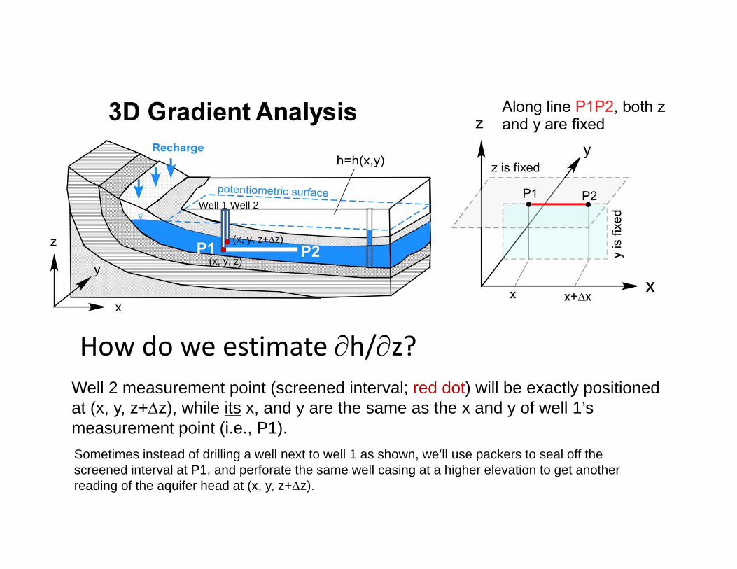
How do we estimate h/z?Well 2 measurement point (screened interval; red dot) will be exactly positioned at (x, y, z+z), while its x, and y are the same as the x and y of well 1’s measurement point (i.e., P1).

Well 1 Well 2

(x, y, z+z)

(x, y, z)

Sometimes instead of drilling a well next to well 1 as shown, we’ll use packers to seal off the screened interval at P1, and perforate the same well casing at a higher elevation to get another reading of the aquifer head at (x, y, z+z).

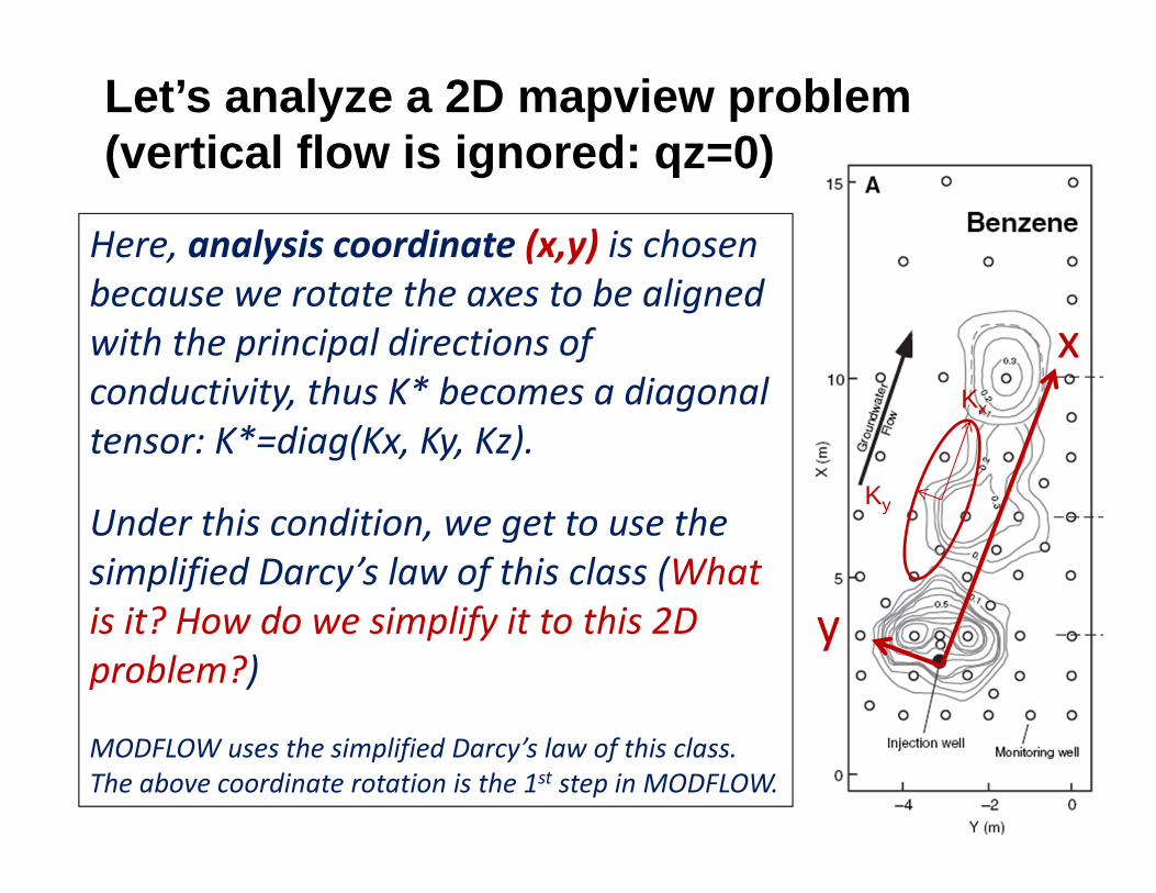
Here, analysis coordinate (x,y) is chosen because we rotate the axes to be aligned with the principal directions of conductivity, thus K* becomes a diagonal tensor: K*=diag(Kx, Ky, Kz).

Under this condition, we get to use the simplified Darcy’s law of this class (What is it? How do we simplify it to this 2D problem?)

MODFLOW uses the simplified Darcy’s law of this class. The above coordinate rotation is the 1st step in MODFLOW. 

x

y

Kx

Ky

Let’s analyze a 2D mapview problem (vertical flow is ignored: qz=0)

x

y

q

Darcy’s flux of the aquifer is known: gw is flowing at 10 m/yr towards N30E.

• Within the analysis coordinate (x,y), x is

aligned with N30E, how would you write the Darcy’s flux (q) vector?

• What will this flux be within the “natural coordinate” (S-E; N-W)?

x

y

If q is not known, we use Darcy’s law to find it:

• Within the analysis coordinate (x,y), how do you use the

hydraulic heads from the pizeometers to evaluate h/x, and h/y?

Hint: where are the wells that satisfy

the definitions of h/x, h/y?

123

4

5

6

7

Exercise 5 In a 2D transect of the head contours, calculate qx and qz assuming isotropic conductivity (Kx = Kz = 2 m/day). Make a scaled vector sketch of the x and z components of the Darcy flux and the flux vector itself q (Assume: qy = 0). 

Repeat the problem assuming anisotropic conductivity (Kx = 2 m/day, Kz = 0.1 m/day). Discuss how the orientation of qrelates to the head contours in both cases.Here, we assume: principal directions of K* are aligned with the coordinate axes; For a 2D transect, the Darcy’s law is (please review how 3D Darcy’s law is simplified):

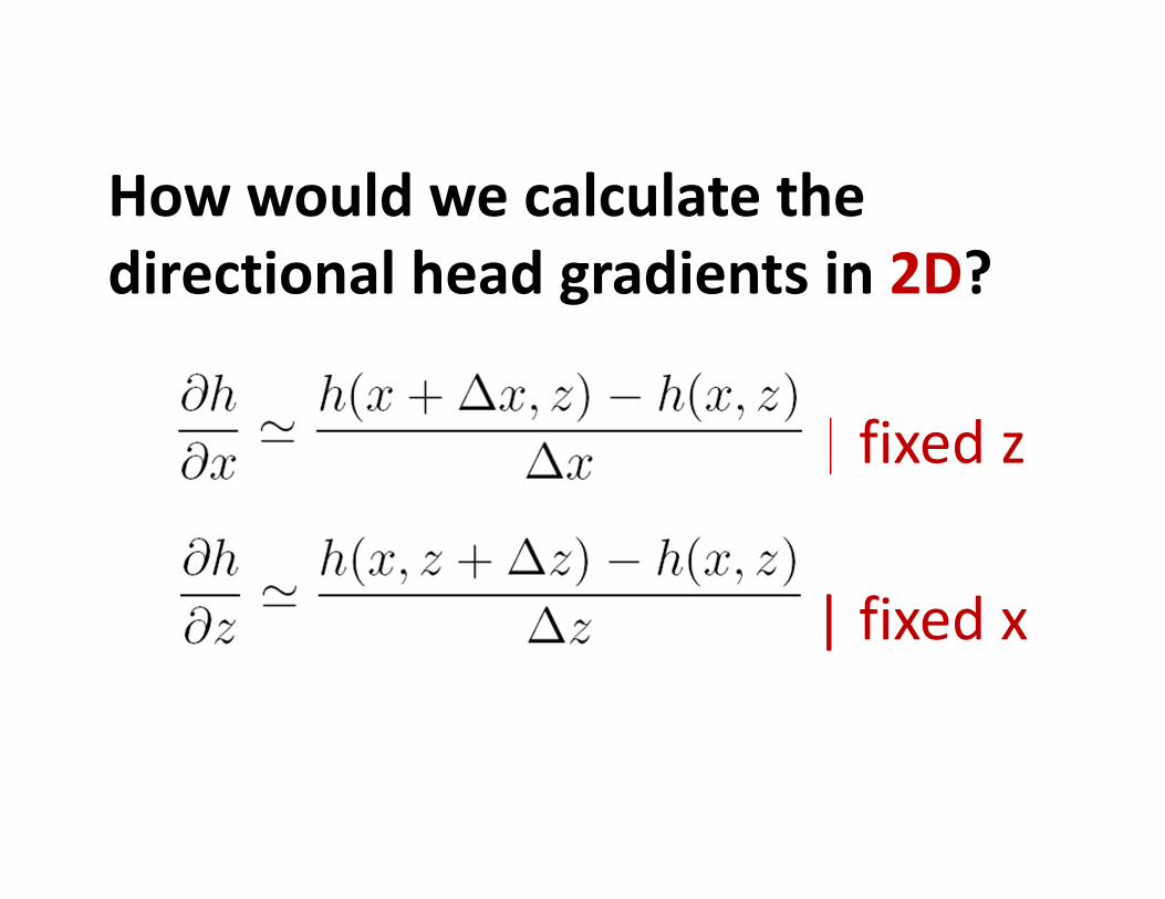
| fixed z

| fixed x

How would we calculate the directional head gradients in 2D?

qx = ‐ Kx (h/x)qz = ‐ Kz (h/z)

(x,z) (x+x,z)

(x,z+z)

(x,z)

qx = ‐ K (h/x)qz = ‐ K (h/z)

• Darcy flux vector is perpendicular to the head contours (or equipotential lines): q points from higher head towards lower head.

• q has the opposite direction with the head gradient vector: I={h/x, h/z}T,  I points from lower head to higher head (please plot I on previous plot);

• What about the GW streamlines, i.e, macroscopic fluid flow pathways (please plot on previous plot)?

When K is isotropic (a scalar):

qx = ‐ Kx (h/x)qz = ‐ Kz (h/z)

(x,z) (x+x,z)

(x,z+z)

(x,z)

Please plot: q; I; and streamlines

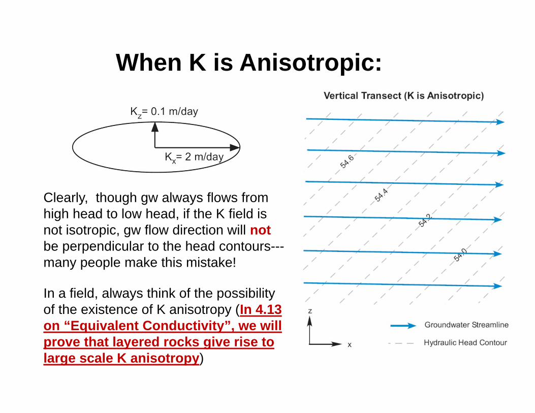
Clearly, though gw always flows from high head to low head, if the K field is not isotropic, gw flow direction will notbe perpendicular to the head contours---many people make this mistake!

In a field, always think of the possibility of the existence of K anisotropy (In 4.13 on “Equivalent Conductivity”, we will prove that layered rocks give rise to large scale K anisotropy)

When K is Anisotropic:

“Missing Plume”:

GW is contaminated at an undisclosed site;

Engineers first assumed isotropic K streamline perpendicular to head contours plume migrates down head gradient; Install wells to intersect the plume for treatment, but no plume is found along the imagined flow path;

Buried “channels” in the aquifer K is anisotropic actual flow path is different (blue streamlines) real plume.

Ky

Plainview

Kx

When conductivity is anisotropic (K* becomes a tensor), Darcy flux is not perpendicular to the head contours, nor it is in the opposite direction of the head gradient vector.

Isotropic (K is scalar): K acts to stretch I to form q; “‐” results in opposite direction of q and I

Anisotropic (K* is tensor): K* acts to both stretch and rotate I to form q

When K is Anisotropic:

In summary, in hydrological analysis:(1) Set up your analysis coordinate: to use the diagonal tensor of K* (of 

this class), coordinate must be aligned with K* principle directions;(2) Set head datum somewhere  z & head become defined;(3) Within the coordinate, evaluate head gradient components: dh/ds

(1D), or h/x, h/y, h/z (2D or 3D; partial sign). Pick 2 points in the aquifer (usually where the well screens are), find their heads (water level inside wells measuring aquifer heads at the well screens), and calculate the gradient (use definition)

(4) Within your coordinate, find Darcy flux components: qx, qy, qzwhich are linked to head gradient by Darcy’s Law (1, 2 or 3D form);

(5) Within your coordinate, we can map out the Darcy flux (q) which describes the macroscopic flow field (please review how to plot a vector given its components).