GPR Detection of Buried Symmetrically Shaped Mine-likeObjects using Selective Independent Component Analysis

Brian Karlsena, Helge B.D. Sørensena, Jan Larsenb, and Kaj B. Jakobsena

aØrsted•DTU, Technical University of DenmarkØrsteds Plads, Building 348, DK-2800 Kongens Lyngby, Denmark

bInformatics and Mathematical Modelling, Technical University of DenmarkRichard Petersens Plads, Building 321, DK-2800 Kongens Lyngby, Denmark

ABSTRACT

This paper addresses the detection of mine-like objects in stepped-frequency ground penetrating radar (SF-GPR) data as a function of object size, object content, and burial depth. The detection approach is based on aSelective Independent Component Analysis (SICA). SICA provides an automatic ranking of components, whichenables the suppression of clutter, hence extraction of components carrying mine information. The goal of theinvestigation is to evaluate various time and frequency domain ICA approaches based on SICA. The performancecomparison is based on a series of mine-like objects ranging from small-scale anti-personal (AP) mines to large-scale anti-tank (AT) mines. Large-scale SF-GPR measurements on this series of mine-like objects buried in soilwere performed. The SF-GPR data was acquired using a wideband monostatic bow-tie antenna operating inthe frequency range 750MHz − 3.0GHz. The detection and clutter reduction approaches based on SICA aresuccessfully evaluated on this SF-GPR dataset.

Keywords: time and frequency based ICA, Selective ICA, stepped-frequency, features, wideband, bow-tieantenna

1. INTRODUCTION

In recent years the development of signal processing techniques for automatic detection of anti-personal (AP)landmines from sensor signals has received significant interest. This paper focuses on an unambiguous detectionof non-metallic AP-landmines in ground penetrating (GPR) radar signals using independent component analysis(ICA). The detection of non-metallic AP-landmines using a GPR is a non-trivial task due to weak scattering2, 3.Nevertheless, the GPR is widely used as one of the main sensors in state-of-the-art AP-landmine detectionsystems1. Most AP-landmines are buried close to the surface of the ground, and automatic object detection ishampered by the strong clutter from the ground surface. In general, the clutter that effects GPR can be definedas signals that are unrelated to the target scattering characteristics but occupy the same frequency band asthe targets. Clutter can be caused by multiple reflections, e.g., in the antenna, between the antenna and theground surface, and the non-landmine targets buried in the ground. However, on the detection of shallow buriednon-metallic AP-landmines the ground surface clutter is the strongest and most significant clutter. Hence, toincrease the detection of shallow buried objects, like the non-metallic AP-landmines, it is necessary to deployproper clutter reduction and detection methods.

The literature suggests a number of clutter reduction and detection methods, such as likelihood ratio testing4,parametric system identification5–8, wavelet packet decomposition9, 10, subspace techniques11–15, and simplemean subtraction2. However, many of these fail to detect shallow buried AP-landmines, mostly because of thestatistical nature of the clutter, e.g., the ground surface is not perfectly flat nor even relative smooth. Anotherproblem is that many of the methods use reference-signal estimates or templates of the signature of the target orthe clutter. These reference-signals and templates are used to remove the signal that are unrelated to the targetsignal signatures. However, a target signal which has little correlation with the reference-signals or templates

Further author information on: BK : brk@oersted.dtu.dk, www.oersted.dtu.dk; HBDS : hbs@oersted.dtu.dk,www.oersted.dtu.dk; JL: jl@imm.dtu.dk, www.imm.dtu.dk/˜jl; KBJ : kbj@oersted.dtu.dk, www.oersted.dtu.dk

may not be detected, hence, be classified as clutter. Further, the approaches are also often sensitive to unknowndisturbances in the soil and in the target and clutter signal signatures. This is in particular a problem in thedetection of weak scatters, like the non-metallic AP-landmine.

To overcome this problem methods based on blind source signal processing techniques are used. In manysignal processing applications the sensor cannot directly measure the signals of interest. However, in generalwe have access to a linear mixture of the signals, where the mixing coefficients are unknown. In this kind of asignal processing problem, we would like to recover the original signals (or sources) in a blind manner withoutknowing the mixing coefficients. This method is known as blind source separation (BSS). Here, the sources arerelated to the underlying mine scatter signals we want to recover. Recently, we have suggested promising BSSmethods12, 13 for clutter reduction and non-metallic AP-landmine detection based on decomposition of the GPRsignals into clutter and landmine signals using principal component analysis (PCA) and independent componentanalysis (ICA). Both methods are unsupervised methods, i.e., we do not use explicit knowledge of object type,but use the fact that target and the clutter signals possess different statistical nature and are independent.

In this paper we extent recent work by considering both time-domain and frequency-domain GPR based ICAapproaches. Further, we suggest a component selection technique for enhanced identification of non-metallicAP-landmines. In Section 2 we give a review on the proposed ICA approach for GPR signals. In section 3 weextent the ICA approach with different mixture models for GPR signals. A scheme for selection of relevant ICAcomponents of non-metallic AP-landmines is presented in section 4. Finally, section 5 provides a comparativestudy of the presented methods, which are tested on GPR signals collected at an indoor GPR measurementfacility at the Technical University of Denmark.

2. INDEPENDENT COMPONENT ANALYSIS OF GPR SIGNALS

The most general BSS problem can be formulated as follows. We observe the output of a linear or nonlinearsystem, where its inputs are generated from a number of source signals. An example of such a system couldbe a GPR-system, where the source signals are the target and clutter signals, and the received GPR signalsare the output of the system which is a mixture of the source signals given by the target and clutter signals.In the application of clutter reduction and target detection, one would like to separate the source signals intotarget signal sources and clutter signal sources, and then use the target signal sources for detection. Using BSS,the separation can be done in a blind manner if we assume that the source signals are mutually independent.The independence assumption is referred to as ICA. Hence, in the application of landmine detection using GPRwe decompose the received GPR signals, into independent components, i.e., independent source signals. Someof these components will mainly include clutter signals and others mainly landmine signals. By removal ofthe independent components that forms the clutter signal space, it is possible to enhance the detection of thelandmines.

There exist many different mathematical or physical models in the mixing process of unknown independentsource signals. Therefore, a given mixture model depends on the specific application. In this paper we focuson the blind separation of noise-free linear instantaneous mixtures of independent source signals. This mixturemodel has shown good results in the application of landmine detection using GPR. The linear instantaneousmixture model can be expressed by

X = AS =

K∑

i=1

ais>

i and Xp,n =

K∑

i=1

Ap,iSi,n, (1)

where X ={Xp,n} = [x1,x2, · · · ,xN ] is a P ×N dimensional signal matrix that spans the space of the receivedGPR signals, A = {Am,i} = [a1,a2, · · · ,aK ] is a general mixing matrix of dimension P ×K and S = {Si,n} =[s1, s2, · · · , sK ]> is a set of K independent source signals. S has the dimension K × N . P is the number ofsensors, N the number of samples in each sensor signal, and K the number of independent sources. That is,from the linear mixture model expressed by eq. (1) the ICA forms a subspace of independent source signals, S.In other words, ICA decomposes X into K independent source signals, S.

In order to recover the original independent source signals, S, from the observed mixture, X, we use a simplelinear separating system expressed by

S = WX, (2)

where S = {Si,n} = [s1, s2, · · · , sK ]> is the K × N dimensional matrix of K estimated source signals, and W

is an estimated unmixing matrix, which is the pseudo inverse of A, W ] = A. That is, from eq. (2) we areable to estimate A and S up to scaling factors and permutations of the source signals. In this paper we do notfocus on algorithms for estimating A and S. However, the literature provides a number of algorithms16, 17. Somedeploy higher (or lower) order moments of non-Gaussian sources, whereas others use the correlation of the sourcesignals. We deploy a member from each family: the widely used Bell-Sejnowski (BS-ICA) algorithm using naturalgradient learning18, and the Molgedey-Schuster19, 20 (MS-ICA) algorithm using the implementations provided inthe DTU-Toolbox21.

Pre-whitening of the GPR signals is optional in order to improve convergence speed for ill-conditioned prob-lems. We provide PCA which is a orthogonal transform and decorrelation approach for pre-whitening of theGPR signals. This method can also be used in BSS problems for source separation. Here, the major differencefrom ICA is that the sources from PCA, the so called principal components, are constrained to be uncorrelatedrather than mutually independent. As input to the ICA we first employ the PCA on the GPR signals. PCA canbe executed using singular value decomposition (SVD) expressed by

X = UDV > =

N∑

i=1

uiDi,iv>

i and Xp,n =

N∑

i=1

Up,iDi,iVn,i, (3)

where the P × N matrix U = {Up,i} = [u1,u2, · · · ,uN ] and the N ×N matrix V = {Vn,i} = [v1,v2, · · · ,vN ]

represent orthonormal basis vectors, i.e., eigenvectors of the symmetric matrices XXT and XTX, respectively.D = Di,i is an N × N diagonal matrix of singular values ranked in decreasing order, as shown by Di,i ≥Di+1,i+1,∀ i ∈ [1;N − 1]. The SVD identifies a set of uncorrelated time signals, the principal components(PC’s): yi = Di,ivi, enumerated by the component index i = 1, 2, . . . , N and yi = [yi(1), · · · , yi(N)]>. Thedimension of the PCA data set will be K ≤ N . That is, we model X only from non-zero eigenvalues22 andfurther have the possibility of projecting onto a subspace. Pre-whitening and subspace projection of X is obtainedby

X = U>

X, (4)

where U = [u1,u2, · · · ,uK ] is P ×K and X is a K ×N matrix. Hence, after pre-whitening and projection theK ×K ICA problem with mixing matrix Φ is

X = ΦS , S = WX = Φ−1U>

X (5)

In the application of landmine detection in GPR signals, the ICA can be used to detect landmines and reduceclutter. By selecting (see further section 4) components which mainly carry mine information, say sk, we canremove clutter. The reconstructed signal space in the original GPR signal space is then

xk = UΦsk (6)

3. THE GPR SIGNAL MATRIX

The signal matrix, X, that spans the signal space of the received GPR signals can be constructed in differentways. Hence four different mixture models based on eqs. (1)-(5).

3.1. Time–Time: Time independence of GPR time signals

The mixture model for time independence of GPR time signals embodies the assumption that the GPR timesignals is a linear mixture of K independent GPR time signal sequences. Hence, we have the linear mixturemodel expressed by X1 = A1S1 = U1Φ1S1, where A1 is a P ×K dimensional mixture matrix, S1 is a K ×Ndimensional set of K independent GPR time signal sequences, and X1 is a P × N dimensional signal matrix

that spans the received GPR time signal X1 = {X1,p,n}, where P is the number of sensor signals. The sensorsignals are given by the GPR time signals, which are received by scanning the GPR above the ground surfacein the x- and y-direction. N is the number of samples in each of the received GPR time signals. Hence, x1,p(n)is sample n of the GPR time signal received at the antenna located at position (x, y) =

((i− 1)4x , (j − 1)4y

),

where i = 1, 2, · · · , I, and j = 1, 2, · · · , J . 4x and 4y are the antenna location step size in the x- and y-direction,respectively, and p = i + (j − 1)I. I and J are the numbers of antenna locations in the x- and y-direction,respectively.

3.2. Time–Spatial: Space independence of GPR time signals

The mixture model for space independence of GPR time signals embodies the assumption that the GPR timesignals is a linear mixture of K independent xy-images. Hence, we have the linear mixture model expressed byX2 = A2S2 = U2Φ2S2, where A2 is a K ×K dimensional mixture matrix, S2 is a K ×P dimensional set of Kindependent GPR xy-images and X2 is a N ×P dimensional signal matrix that spans the GPR time signal spaceobserved where P is the number of sensor signals and N is the number of time samples. That is, X2 = X>

1 .The next two models we are considering frequency models of the GPR signals. Since stepped-frequency GPRmeasurement is a complex frequency representation we could also consider the ICA a decomposing the receivedspectrum into characteristic mine and clutter spectra. For simplicity we will consider only the magnitudespectrum hence using real ICA models.

3.3. Frequency–Frequency: Frequency independence of GPR frequency signals

The mixture model for frequency independence of the GPR frequency spectra embodies the assumption thatthe GPR frequency spectra is a linear mixture of K independent frequency spectra. Hence, we have the linearmixture model expressed by X3 = A3S3 = U3Φ3S3, where A3 is a K ×K dimensional mixture matrix, S3 isa K ×N dimensional set of K independent GPR magnitude frequency spectra and X3 is a P ×N dimensionalsignal matrix that spans the GPR frequency spectra observed. For this mixture model X3 is constructed asX3 = {X3,p,n} where P is the number of sensor signals, which are received by scanning the GPR above theground surface in the x- and y-direction. N is the number of frequencies in each of the received frequency spectra,and x1,i(n) is the amplitude of the frequency bin n in the GPR frequency spectrum received at the GPR antennalocated at position (x, y) =

((i− 1)4x, (j − 1)4y

), where i = 1, 2, · · · , I, and j = 1, 2, · · · , J . 4x and 4y are the

antenna location step size in the x- and y-direction, respectively, and p = i+ (j − 1)I. I and J is the number ofantenna locations in the x- and y-direction, respectively.

3.4. Frequency–Spatial: Space independence of GPR time frequency signals

The mixture model for space independence of GPR frequency signals embodies the assumption that the GPRfrequency signals is a linear mixture of K independent magnitude GPR frequency xy-images. This model is thetranspose of mixture model 3, thus X4 = X>

3 . The linear mixture model is expressed by X4 = A4S4 = U4Φ4S4,where A4 is a K × K dimensional mixture matrix, S4 is a K × P dimensional set of K independent GPRmagnitude frequency xy-images and X4 is a N × P dimensional signal matrix that spans the observed GPRmagnitude frequency signal space, where P is the number of sensor signals and N is the number of frequencybins.

4. SCHEME FOR SELECTIVE INDEPENDENT COMPONENT ANALYSIS

The ranking and selection of relevant components can be done in many different ways. We suggest a simplemethod based on a measure of the fourth-order statistics of the extracted independent sources23. Similar to thePCA where the orthogonal sources are sorted by the variance (second-order statistics) we can sort the independentsources according to non-Gaussianity. It turns out that independent components with a high contrast and withhigh non-Gaussian structure carry mine information whereas clutter components are more Gaussian. A way toestimate non-Gaussianity is by evaluating the normalized kurtosis,

κ4(si) =E{|si|

4}

E2{|si|2}− 3. (7)

Sorting the independent according to normalized kurtosis and selecting components with κ4 > δ, where δ > 0 isa given threshold, provides the selection of mine components.

5. EXPERIMENTS AND RESULTS

In order to get an idea about the effectiveness of the proposed ICA mixture models and the scheme for theranking of the IC’s for clutter reduction and non-metallic AP-landmine detection, we have performed studies onfield-test stepped-frequency GPR signals. The field-test data was collected using a monostatic bow-tie antennaoperating in the frequency range 750MHz−3.0GHz. The data was acquired using a HP8753A network analyzer.In a measurement area of 101 cm × 101 cm non-metallic cylinders of different size and with different contentof non-metallic material were buried in different depths. In table 1 are the technical specification of the the

Target Cyl. no. 1 Cyl. no. 2 Cyl. no. 3 Cyl. no. 4

Diameter 15 cm 15 cm 5 cm 5 cmHeight 5 cm 5 cm 5 cm 5 cmContent Air Beeswax Air BeeswaxContainer Plastic Plastic Plastic Plastic

Table 1. Test objects used for testing the proposed ICA mixture models.

buried non-metallic cylinders listed. Half of them were with no contents (air) and the other half were filledwith beeswax. All the cylinders were buried in the center of the measurement area in relative dry soil 0 cm,5 cm, and 10 cm below the surface. The relative permittivity of the soil was εr = 2.8, and was estimated usinga loop antenna24. The measurement area was scanned and SF-GPR signals were collected at every antennapositions located (4x = 1 cm) × (4y = 1 cm) from each other. The number of frequencies were 601. That is,4f = 3.75MHz. Before the ICA methods were deployed on the SF-GPR data, the SF-GPR data were noisereduced by smoothing the discrete spectrum of 601 frequencies measured at each GPR antenna location. Forthe Time–Time and Time–Space ICA mixture models the frequency-domain data were down-modulated to thebase-band and Fourier-transformed to the time-domain using a sampling frequency of 30.72GHz.

The four ICA mixture models were tested on the SF-GPR data using BS-ICA and MS-ICA. In figure 1 tofigure 8 are selected results shown for BS-ICA and MS-ICA. The selected results shown are results from cylinderno. 1 and cylinder no. 2. To get the results we first removed the mean value from the SF-GPR signals and thendeployed PCA as pre-whitening (see eq.4). After PCA the most noisy PCA subspaces were removed. From thePCA we ended up with 30-70 subspaces describing 100% of the SF-GPR data depending on the data example.We kept the first 20 PCA subspaces and used these subspaces as input for the BS-ICA and MS-ICA. Afterapplying BS-ICA and MS-ICA we ranked the IC’s after highest normalized kurtosis (see section 4). Within theIC’s with highest kurtosis we did the selection of relevant IC’s for reconstruction. In this way we have reducedthe PCA subspace of up to 70 subspaces down to about 5 selective IC subspaces containing mainly landmine-likeinformation.

As a performance measure on the reduction of clutter and detection, the area under the ROC curve is used.For all the considered examples the area under the ROC curve is listed in table 2. The closer to 1 the area underthe ROC curve is the better the performance we have. From this it is clear that some of the ICA mixture modelsare better than others. In general, the ROC curve shows the performance of a particular detector or classifier.However, in this paper the ROC curves shown, and the area under the ROC curves, are more a measure on theclutter reduction, i.e., the signal-to-clutter radio. That is, in the results we know were the landmine is buried.Hence, by a threshold on the sum-variance image (Ii,j = diag(x2

k)) of each reconstructed signal matrices we canclassify the image into clutter and landmine from the knowledge on were the landmines are buried. By changingthe threshold the ROC curve is constructed. That is, the ROC curve is more a measure on how good the selectedlandmine signals are separated from the clutter, rather than a measure in general on classification or detection.

5.1. Time–Time Results

In the Time–Time ICA mixture model (X1) we seek for time independence of time signals. In figure 1 and 2 aretwo examples of extracted IC’s from the ICA mixture model shown. In figure 1 are results for BS-ICA shown,and in figure 2 are results for MS-ICA shown. For both examples the first 6 IC’s (time signal sequences) andthe corresponding mixture coefficients (eigenimages) are shown. From the results of the BS-ICA we have rather

peaked IC’s, and localized signatures in some of the eigenimages. In particular source no. 2 and no. 6 showlandmine-like signatures in the eigenimages. Hence, they are used for reconstruction of the clutter reduced signalmatrix. Further, the IC’s peak at a depth that corresponds to the burial depth of the cylinder (0 cm = 2.5 ns).The results from the MS-ICA are different from the BS-ICA. This is due to fact that MS-ICA is based ondecorrelation of delayed time signals. Therefore, we get more correlated IC’s which are independent from eachother. Moreover, BS-ICA gives as non-Gaussian signals as possible. Hence, they are rather peaked. In general,the GPR time signals are peaked and not as correlated as the sources from the MS-ICA. Therefore, BS-ICAgives satisfactory results. This can also be seen from the results listed in table 2. The results show that BS-ICAdeployed on the ICA mixture model gives a satisfactory separation and detection on both cylinder no. 1 andno. 2.

5.2. Time–Spatial Results

In the Time–Spatial ICA mixture model (X2) we seek for spatial independence of time signals. In figure 1 and2 are two examples of extracted IC’s for the ICA mixture model shown. In figure 1 are results for BS-ICAshown and in figure 2 are results for MS-ICA shown. For both examples the first 6 IC’s (eigenimages) and thecorresponding mixture coefficients (time signal sequences) are shown. From the BS-ICA we get rather peakedIC’s. Hence we have IC’s with strong landmine signatures. In particular component no. 1 shows strong landmine-like signatures. The corresponding mixer coefficients, which in this case are time signal signatures also showstrong landmine-like signatures, i.e., they are peaked. The results from MS-ICA are non-satisfactory. Due to thefact that the buried cylinders are weak scatters it is hard for MS-ICA to enhance, i.e., through decorrelation, thespatial signatures without enhancing the clutter. Hence, no clutter reduction. From the results shown in table 2it is clear that ICA mixture model gives non-satisfactory results for MS-ICA on weak scatters. However, on astrong scatter (cyl. no. 2) both BS-ICA and MS-ICA have a satisfactory performance.

5.3. Frequency–Frequency Results

In the Frequency–Frequency ICA mixture model (X3) we seek for frequency independence of the frequencyspectra. In figure 1 and 2 are two examples of extracted IC’s for the ICA mixture model shown. In figure 1are results for BS-ICA shown and in figure 2 are results for MS-ICA shown. For both examples the first 6 IC’s(frequency spectra) and the corresponding mixture coefficients (eigenimages) are shown. From the BS-ICA weget rather peaked IC’s. However, the physical signature of the frequency spectra is not peaked signals. Hence,the BS-ICA will extract IC’s that may have non-physical signatures. In this example it is clear that we do notextract any landmine-like information. However, the MS-ICA is able to extract some landmine information.Because of the fact that the frequency spectra measured at each SF-GPR antenna position is rather correlatedwe get IC’s that are similar to the real frequency spectra signature. Hence, good separation. From the resultsshown in table 2 it is clear that the ICA model gives a satisfactory performance on weak scatters for MS-ICAonly. For strong scatters both MS-ICA and BS-ICA shows good results.

5.4. Frequency–Spatial Results

In Frequency–Spatial ICA mixture model (X4) we seek for spatial independence of frequency spectra. In figure 1and 2 are two examples of extracted sources for the ICA mixture model shown. In figure 1 are results for BS-ICAshown and in figure 2 are results for MS-ICA shown. For both examples the first 6 IC’s (eigenimages) and thecorresponding mixture coefficients (frequency spectra) are shown. From the BS-ICA we get rather peaked IC’s.Hence, we have strong landmine signatures in the eigenimages. In particular component no. 1 shows stronglandmine-like signatures. The frequency spectra shows a rather physical signature. The results from the MS-ICA are similar. From the results shown in table 2 it is clear that the ICA mixture model gives a satisfactoryperformance on weak and strong scatters for both MS-ICA and BS-ICA.

Frequency–Spatial, BS-ICA Frequency–Frequency, BS-ICAno. 1 no. 2 no. 3

no. 4 no. 5 no. 6

no. 1 no. 2 no. 3

no. 4 no. 5 no. 6

1 2 3

−5

0

5

no. 1

1 2 3

−10

0

10

no. 2

1 2 3

−5

0

5

no. 3

1 2 3

−4

−2

0

no. 4

1 2 3

−1

0

1

2no. 5

1 2 3−10

−5

0

5

no. 61 2 3

0

5

10

no. 1

1 2 3

−5

0

5

no. 2

1 2 3−10

−5

0

no. 3

1 2 3

−10

−5

0

no. 4

1 2 30

5

10

no. 5

1 2 3−4−2

0246

no. 6

f [GHz] f [GHz]Time-Spatial, BS-ICA Time–Time, BS-ICA

no. 1 no. 2 no. 3

no. 4 no. 5 no. 6

no. 1 no. 2 no. 3

no. 4 no. 5 no. 6

0 5

−2

0

2

no. 1

0 5−5

0

5

no. 2

0 5−2

0

2

no. 3

0 5−5

0

5

no. 4

0 5

−1

0

1

no. 5

0 5−4

−2

0

2

4no. 6

0 5−10

0

10

no. 1

0 5−10

0

10

no. 2

0 5−10

0

10

no. 3

0 5−10

−5

0

5

no. 4

0 5−10

−5

0

5

no. 5

0 5

−10

0

10no. 6

t [ns] t [ns]

Figure 1. Results from BS-ICA deployed on the four ICA mixture models. The SF-GPR data used are measurements oncylinder no. 2 buried 0 cm. Notice that for BS-ICA the Frequency-Frequency ICA mixture model have a non-satisfactoryseparation of the SF-GPR frequency signals. This is due to the fact that the frequencies in the frequency spectrum arenot in general independent from each other.

Frequency–Spatial, MS-ICA Frequency–Frequency, MS-ICAno. 1 no. 2 no. 3

no. 4 no. 5 no. 6

no. 1 no. 2 no. 3

no. 4 no. 5 no. 6

1 2 3

−1

0

1

no. 1

1 2 3−0.4

−0.2

0

0.2

no. 2

1 2 3−0.4

−0.2

0

0.2no. 3

1 2 3

−0.5

0

0.5no. 4

1 2 3−2

0

2

no. 5

1 2 3

−0.5

0

0.5

no. 61 2 3

−0.05

0

0.05

no. 1

1 2 3−0.05

0

0.05

no. 2

1 2 3−0.05

0

0.05

no. 3

1 2 3−0.05

0

0.05

no. 4

1 2 3−0.05

0

0.05

no. 5

1 2 3−0.05

0

0.05

no. 6

f [GHz] f [GHz]Time–Spatial, MS-ICA Time–Time, MS-ICAno. 1 no. 2 no. 3

no. 4 no. 5 no. 6

no. 1 no. 2 no. 3

no. 4 no. 5 no. 6

0 5−5

0

5no. 1

0 5−4−2

024

no. 2

0 5

−2

0

2

no. 3

0 5−5

0

5no. 4

0 5

−2

0

2

no. 5

0 5

−4

−2

0

2

4

no. 6 0 5−0.1

0

0.1no. 1

0 5

−0.1

0

0.1

no. 2

0 5−0.1

−0.05

0

0.05

no. 3

0 5−0.1

0

0.1

no. 4

0 5−0.1

0

0.1

no. 5

0 5−0.1

0

0.1

no. 6

t [ns] t [ns]

Figure 2. Results from MS-ICA deployed on the four ICA mixture models. The SF-GPR data used are measurementson the cylinder no. 2 buried 0 cm under the surface. Notice that the MS-ICA for the Time-Spatial ICA mixture modelhave a non-satisfactory performance due to weak scatters.

Frequency-Spatial, BS-ICA

Beeswax, z = 0 cm Air, z = 0 cm ROC

f = 1.5 GHz

f = 1.95 GHz

f = 1.5 GHz

f = 1.95 GHz

f = 1.3 GHz

f = 1.95 GHz

f = 1.3 GHz

f = 1.95 GHz

0 20 40 60 80 1000

20

40

60

80

100

PF [%]

PD

[%]

Raw BeeswaxRaw AirBS BeeswaxBS Air

Figure 3. The first row shows the raw SF-GPR data at the frequencies 1.5GHz and 1.95GHz for cyl. no. 1 buried 0 cmand 1.3GHz and 1.95GHz for cyl. no. 2 buried 0 cm. The second row shows the reconstructed data using BS-ICA on theFrequency-Spatial ICA mixture model. The images and the ROC curves show that the detection is improved.

Frequency-Spatial, BS-ICA

Beeswax, z = −10 cm Air, z = −10 cm ROC

f = 1.5 GHz

f = 1.95 GHz

f = 1.5 GHz

f = 1.95 GHz

f = 1.3 GHz

f = 1.95 GHz

f = 1.3 GHz

f = 1.95 GHz

0 20 40 60 80 1000

20

40

60

80

100

PF [%]

PD

[%]

Raw BeeswaxRaw AirBS BeeswaxBS Air

Figure 4. The first row shows the raw SF-GPR data at the frequencies 1.5GHz and 1.95GHz for cyl. no. 1 buried 10 cmand 1.3GHz and 1.95GHz for cyl. no. 2 buried 10 cm. The second row shows the reconstructed data using BS-ICA onthe frequency-Spatial ICA mixture model. The images and the ROC curves show that the detection is improved.

Frequency-Frequency, MS-ICA

Beeswax, z = 0 cm Air, z = 0 cm ROC

f = 1.5 GHz

f = 1.95 GHz

f = 1.5 GHz

f = 1.95 GHz

f = 1.3 GHz

f = 1.95 GHz

f = 1.3 GHz

f = 1.95 GHz

0 20 40 60 80 1000

20

40

60

80

100

PF [%]

PD

[%]

Raw BeeswaxRaw AirMS BeeswaxMS Air

Figure 5. The first row shows the raw SF-GPR data at the frequencies 1.5GHz and 1.95GHz for cyl. no. 1 buried 0 cmand 1.3GHz and 1.95GHz for cyl. no. 2 buried 0 cm. The second row shows the reconstructed data using MS-ICA onthe frequency-frequency ICA mixture model. The images and the ROC curves show that the detection is improved.

Time-Spatial, BS-ICA

Beeswax, z = 0 cm Air, z = 0 cm ROC

t = 1.3 ns t = 2.0 ns

t = 1.3 ns t = 2.0 ns

t = 1.3 ns t = 2.0 ns

t = 1.3 ns t = 2.0 ns

0 20 40 60 80 1000

20

40

60

80

100

PF [%]

PD

[%]

Raw BeeswaxRaw AirBS BeeswaxBS Air

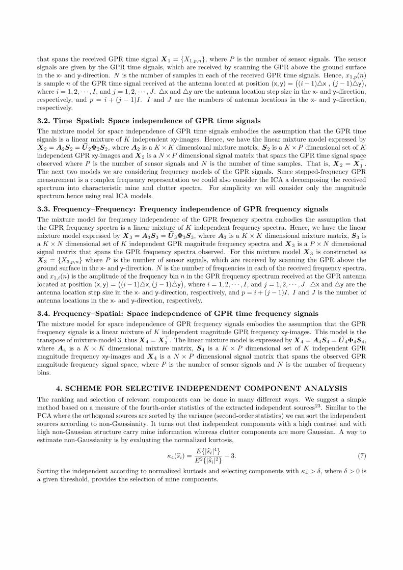
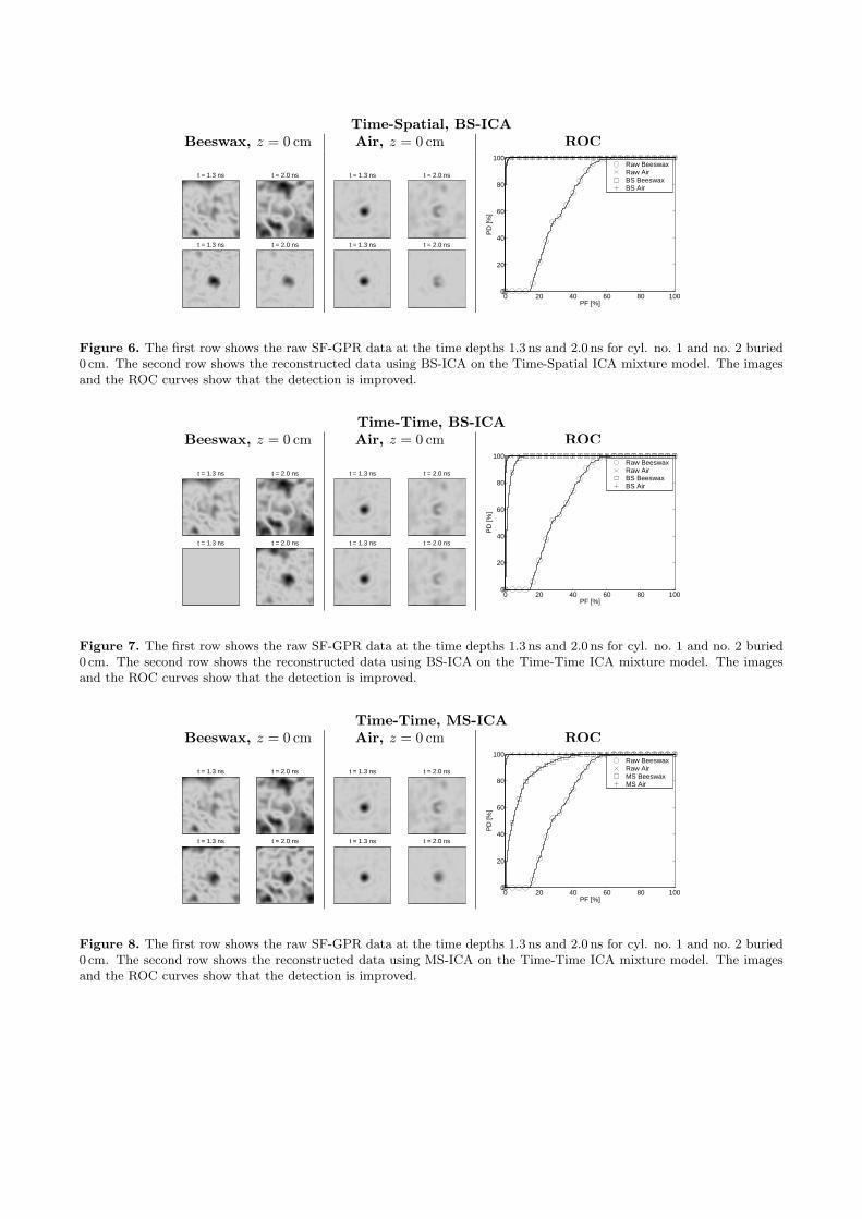
Figure 6. The first row shows the raw SF-GPR data at the time depths 1.3 ns and 2.0 ns for cyl. no. 1 and no. 2 buried0 cm. The second row shows the reconstructed data using BS-ICA on the Time-Spatial ICA mixture model. The imagesand the ROC curves show that the detection is improved.

Time-Time, BS-ICA

Beeswax, z = 0 cm Air, z = 0 cm ROC

t = 1.3 ns t = 2.0 ns

t = 1.3 ns t = 2.0 ns

t = 1.3 ns t = 2.0 ns

t = 1.3 ns t = 2.0 ns

0 20 40 60 80 1000

20

40

60

80

100

PF [%]

PD

[%]

Raw BeeswaxRaw AirBS BeeswaxBS Air

Figure 7. The first row shows the raw SF-GPR data at the time depths 1.3 ns and 2.0 ns for cyl. no. 1 and no. 2 buried0 cm. The second row shows the reconstructed data using BS-ICA on the Time-Time ICA mixture model. The imagesand the ROC curves show that the detection is improved.

Time-Time, MS-ICA

Beeswax, z = 0 cm Air, z = 0 cm ROC

t = 1.3 ns t = 2.0 ns

t = 1.3 ns t = 2.0 ns

t = 1.3 ns t = 2.0 ns

t = 1.3 ns t = 2.0 ns

0 20 40 60 80 1000

20

40

60

80

100

PF [%]

PD

[%]

Raw BeeswaxRaw AirMS BeeswaxMS Air

Figure 8. The first row shows the raw SF-GPR data at the time depths 1.3 ns and 2.0 ns for cyl. no. 1 and no. 2 buried0 cm. The second row shows the reconstructed data using MS-ICA on the Time-Time ICA mixture model. The imagesand the ROC curves show that the detection is improved.

Cyl. contents: Beeswax Cyl. contents: Air

Mode z Raw PCA MS-ICA BS-ICA Raw PCA MS-ICA BS-ICA

0 cm 0.6170 0.9921/1 0.9980/1 0.9990/1 0.9996 0.9981/4 0.9957/2 0.9999/2F-S -5 cm 0.7137 0.9557/2 0.7499/1 0.9995/1 0.9864 0.9993/2 0.9904/2 0.9973/2

-10 cm 0.9363 0.8919/1 0.9662/3 0.9989/1 0.9962 0.9996/2 0.9831/2 0.9994/2

0 cm 0.6170 0.9921/1 0.9949/2 ——– 0.9996 0.9981/4 0.9999/6 0.9999/9F-F -5 cm 0.7137 0.9557/2 0.9241/4 ——– 0.9962 0.9993/2 0.9988/4 0.9880/7

-10 cm 0.9363 0.8919/1 0.9791/1 ——– 0.9962 0.9996/2 0.9997/5 0.9648/9

0 cm 0.7013 0.9843/1 ——– 0.9986/1 0.9993 0.9999/1 ——– 0.9999/2T-S -5 cm 0.6705 0.9104/2 ——– 0.9994/1 0.9918 0.9911/3 ——– 0.9985/2

-10 cm 0.9374 0.9643/1 0.9498/5 0.9985/1 0.9751 0.9981/3 ——– 0.9994/2

0 cm 0.7013 0.9843/1 0.9210/3 0.9828/3 0.9993 0.9999/1 0.9999/9 0.9994/5T-T -5 cm 0.6705 0.9104/2 0.9355/2 0.9506/2 0.9918 0.9911/3 0.9955/7 0.9986/3

-10 cm 0.9374 0.9643/1 ——– ——– 0.9751 0.9981/3 0.9911/5 0.9997/5

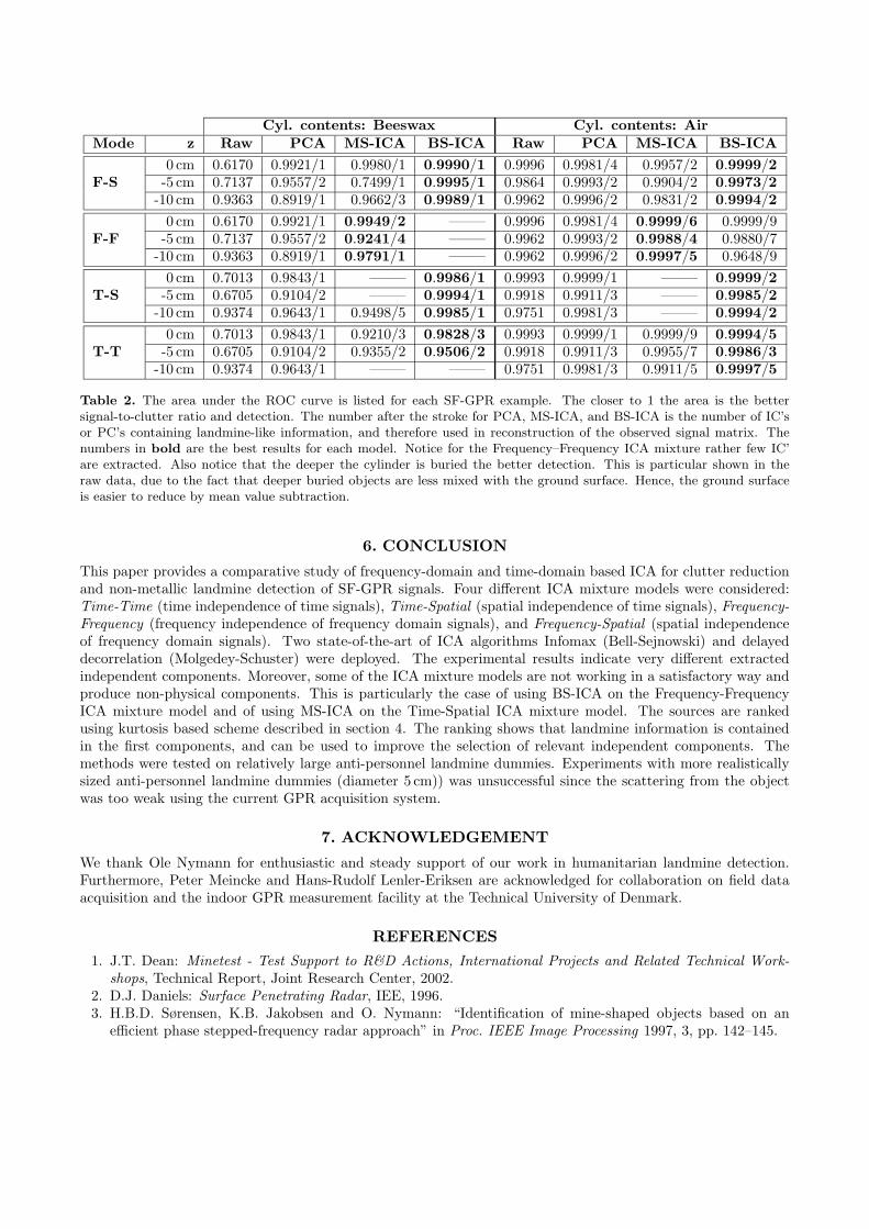
Table 2. The area under the ROC curve is listed for each SF-GPR example. The closer to 1 the area is the bettersignal-to-clutter ratio and detection. The number after the stroke for PCA, MS-ICA, and BS-ICA is the number of IC’sor PC’s containing landmine-like information, and therefore used in reconstruction of the observed signal matrix. Thenumbers in bold are the best results for each model. Notice for the Frequency–Frequency ICA mixture rather few IC’are extracted. Also notice that the deeper the cylinder is buried the better detection. This is particular shown in theraw data, due to the fact that deeper buried objects are less mixed with the ground surface. Hence, the ground surfaceis easier to reduce by mean value subtraction.

6. CONCLUSION

This paper provides a comparative study of frequency-domain and time-domain based ICA for clutter reductionand non-metallic landmine detection of SF-GPR signals. Four different ICA mixture models were considered:Time-Time (time independence of time signals), Time-Spatial (spatial independence of time signals), Frequency-Frequency (frequency independence of frequency domain signals), and Frequency-Spatial (spatial independenceof frequency domain signals). Two state-of-the-art of ICA algorithms Infomax (Bell-Sejnowski) and delayeddecorrelation (Molgedey-Schuster) were deployed. The experimental results indicate very different extractedindependent components. Moreover, some of the ICA mixture models are not working in a satisfactory way andproduce non-physical components. This is particularly the case of using BS-ICA on the Frequency-FrequencyICA mixture model and of using MS-ICA on the Time-Spatial ICA mixture model. The sources are rankedusing kurtosis based scheme described in section 4. The ranking shows that landmine information is containedin the first components, and can be used to improve the selection of relevant independent components. Themethods were tested on relatively large anti-personnel landmine dummies. Experiments with more realisticallysized anti-personnel landmine dummies (diameter 5 cm)) was unsuccessful since the scattering from the objectwas too weak using the current GPR acquisition system.

7. ACKNOWLEDGEMENT

We thank Ole Nymann for enthusiastic and steady support of our work in humanitarian landmine detection.Furthermore, Peter Meincke and Hans-Rudolf Lenler-Eriksen are acknowledged for collaboration on field dataacquisition and the indoor GPR measurement facility at the Technical University of Denmark.

REFERENCES

1. J.T. Dean: Minetest - Test Support to R&D Actions, International Projects and Related Technical Work-shops, Technical Report, Joint Research Center, 2002.

2. D.J. Daniels: Surface Penetrating Radar, IEE, 1996.3. H.B.D. Sørensen, K.B. Jakobsen and O. Nymann: “Identification of mine-shaped objects based on an

efficient phase stepped-frequency radar approach” in Proc. IEEE Image Processing 1997, 3, pp. 142–145.

4. H. Brunzell: “Clutter Reduction and Object Detection in Surface Penetrating Radar,” in Proc. of IEERadar’97, issue 449, 1997, pp. 688–691.

5. J.W. Brooks, L. van Kempen & H. Sahli: “Primary Study in Adaptive Clutter Reduction and BuriedMinelike Target Enhancement from GPR Data,” in Proc. of SPIE, AeroSense 2000: Det. and Rem. Techn.for Mines and Minelike Targets V, vol. 4038, 2000, pp. 1183–1192.

6. L. van Kempen, H. Sahli, E. Nyssen & J. Cornelis: “Signal Processing and Pattern Recognition Methodsfor Radar AP Mine Detection and Indentification,” Det. of Aband. Land Mines, no. 458, pp. 81–85, 1998.

7. A. van der Merwe & I.J. Gupta: “A Novel Signal Processing Technique for Clutter Reduction in GPRMeasurements of Small, Shallow Land Mines,” IEEE Transactions on Geoscience and Remote Sensing vol.38, no. 6, pp. 2627–2637, 2000.

8. J.L. Salvati, C.C. Chen & J.T. Johnson: “Theoretical Study of a Surface Clutter Reduction Algorithm,” inProc. of 1998 IEEE International Geoscience and Remote Sensing, vol. 3, 1998, pp. 1460–1462.

9. D. Carevic: “Clutter Reduction and Target Detection in Ground Penetrating Radar Data Using Wavelets,”in Proc. of SPIE Conf. on Det. and Rem. Tec. for Mines and Minel. Targ. IV, vol. 3710, 1999, pp. 973–997.

10. H. Deng & H. Ling: “Clutter Reduction for Synthetic Aperture Radar Images Using Adaptive WaveletPacket Transform,” in Proc. of IEEE Int. Ant. and Propaga. Soc. Symp., vol. 3, 1999, pp. 1780–1783.

11. A.H. Gynatilaka & B.A. Baertlein: “A subspace decomposition technique to improve GPR imaging of anti-personnel mines,” in Proc. of SPIE, AeroSense 2000: Detect. and Rem. Techn. for Mines and MinelikeTargets V, vol. 4038, 2000, pp. 1008–1018.

12. B. Karlsen, J. Larsen, K.B. Jakobsen, H.B.D. Sørensen & S. Abrahamson: “Antenna Characteristics and Air-Ground Interface Deembedding Methods for Stepped-Frequency Ground Penetrating Radar Measurements,”in Proc. of SPIE, AeroSense 2000: Detect. and Rem. Techn. for Mines and Minelike Targets V, vol. 4038,2000, pp. 1420–1430.

13. B. Karlsen, J. Larsen, H.B.D. Sørensen and K.B. Jakobsen: “Comparison of PCA and ICA based ClutterReduction in GPR Systems for Anti-Personal Landmine Detection,” in Proc. of 11th IEEE Workshop onStatistical Signal Processing, Singapore, Aug. 6–8, 2001, pp. 146–149.

14. A.K. Shaw & V. Bhatnagar: “Automatic Target Recognition Using Eigen-Templates,” in Proc. of SPIEConference on Algorithms for Synthetic Aperture Radar Imagery V, vol. 3370, 1998, pp. 448–459.

15. S.H. Yu & T.R. Witten: “Automatic Mine Detection based on Ground Penetratinig Radar,” in Proc. ofSPIE Conf. on Det. and Rem. Techn. for Mines and Minelike Targets IV, vol. 3710, 1999, pp. 961–972.

16. T.W. Lee: Independent Component Analysis: Theory and Applications Kluwer Academic Publishers, ISBN0792382617, 1998.

17. A. Cichocki and S.-i. Amari: Adaptive Blind Signal and Image Processing: Learning Algorithms and Appli-cations, John Wiley, Chichester, UK, April, 2002.

18. A. Bell & T.J. Sejnowski: “An Information-Maximation Approach to Blind Separation and Blind Deconve-lution,” Neural Computation, vol. 7, pp. 1129–1159, 1995.

19. L. Molgedey & H. Schuster: “Separation of Independent Signals using Time-Delayed Correlations,” PhysicalReview Letters, vol. 72, no. 23, pp. 3634–3637, 1994.

20. L.K. Hansen, J. Larsen & T. Kolenda: “On Independent Component Analysis for Multimedia Signals,” inL. Guan, S.Y. Kung & J. Larsen (eds.) Mult. Image and Vid. Proc. , CRC Press, Ch. 7, pp. 175–199, 2000.

21. T. Kolenda, S. Sigurdsson, O. Winther, L.K. Hansen & J. Larsen: DTU:Toolbox, ISP group, Informaticsand Mathematical Modelling, Technical University of Denmark, http://isp.imm.dtu.dk/toolbox/, 2002.

22. B. Lautrup, L.K. Hansen, I. Law, N. Mørch, C. Svarer & S.C. Strother: “Massive weight sharing: A Curefor Extremely Ill-posed Problems,” in H.J. Herman et al., (eds.) Supercomputing in Brain Research: FromTomography to Neural Networks, World Scientific Pub. Corp. pp. 137–148, 1995.

23. S. Vorobyov & A. Cichocki: “Blind Noise Reduction for Multisensory Signals using ICA and SubspaceFiltering, with Application to EEG Analysis,” in Biological Cybernetics, vol. 86, pp. 293–303, 2002.

24. H.R. Lenler-Eriksen, P. Meincke & E. Jørgensen: “Estiamtion of Constitutive Parameters Using a LoopAntenna,” in Proc. of 2nd International Workshop on Advanced Ground Penetrating Radar (IWAGPR),Delft University of Technology, May 2003.