good regions to deblur - courses.cs.washington.edu
TRANSCRIPT

Good Regions to Deblur
Zhe Hu and Ming-Hsuan Yang
Electrical Engineering and Computer ScienceUniversity of California at Merced{zhu, mhyang}@ucmerced.edu
Abstract. The goal of single image deblurring is to recover both a latentclear image and an underlying blur kernel from one input blurred image.Recent works focus on exploiting natural image priors or additional im-age observations for deblurring, but pay less attention to the influenceof image structures on estimating blur kernels. What is the useful imagestructure and how can one select good regions for deblurring? We for-mulate the problem of learning good regions for deblurring within theConditional Random Field framework. To better compare blur kernels,we develop an effective similarity metric for labeling training samples.The learned model is able to predict good regions from an input blurredimage for deblurring without user guidance. Qualitative and quantita-tive evaluations demonstrate that good regions can be selected by theproposed algorithms for effective image deblurring.
1 Introduction
Motion blur on an image often results from the relative motion between a cameraviewpoint and the scene (e.g., camera shake) at the exposure time. It causessignificant image degradation, especially in the low light conditions where longerexposure time is required. Recovering the latent image from one single blurredimage has been studied extensively with a rich literature. Typically, the blurredimage formation process is modeled as a latent image convolved with a spatial-invariant blur kernel (i.e., the point spread function). Hence, the deblurringprocess is known as a 2D deconvolution problem. When the underlying blurkernel is known or has been accurately estimated, the problem is reduced tonon-blind deconvolution. On the other hand, if the blur kernel is unknown, thedeblurring problem is known as blind deconvolution. The ill-posed nature of thesingle image deblurring setting makes the problem rather difficult.
To deblur an image, it is shown that estimating the blur kernel first and thensolving a non-blind deconvolution problem with the estimated kernel rendersfavorable results [1]. In this case, the performance of the blur kernel estimationdirectly affects the performance of the deblurred results (i.e., the estimated latentimage). That is, one can recover the latent image well if the blur kernel can beaccurately estimated.
For the single image deblurring problem, it is usually advantageous to makefull use of the input blurred image. However, not all pixels of the input blurredimage are informative. Smooth regions, for example, do not contribute much for

2 Good Regions to Deblur
Fig. 1. Different regions lead to different kernel estimations and deblurred results. Thetop left image is the input blurred image with three subwindows selected for estimatingkernels. The other three images are the recovered images and estimated kernels fromthese three subwindows using [2].
estimating the blur kernel. In this paper, we ask “What kind of image features orstructures of a blurred image really help in kernel estimation?” By detecting goodimage features for blur kernel estimation, an accurately estimated blur kernelcan then be used to recover a latent clear image with high visual quality. In [2, 1],it is demonstrated that regions with strong edges tend to yield better deblurringresults. Some of the gradient-based methods favor salient edges with gradientsof specific patterns [3–5]. On the other hand, based on 1D signal examples, itis demonstrated that edges of short length could adversely affect the deblurringresults [5]. In other words, if the whole image is used for image deblurring withoutdeliberate selection of good features, negative impacts are likely to lead to inferiorresults. For this reason and the computational efficiency issue, it is preferableto determine a region, rather than the whole image, for estimating blur kernels.Figure 1 illustrates that different regions may lead to completely different kernelestimation results, and thereby different recovered images. This problem canoften be partly alleviated by manual selection and visual inspection of the results.However, this requires tedious human input for deblurring images. In addition,the questions regarding which regions or what image structures are crucial foraccurate blur kernel estimation remain unanswered.
In this paper, we address these questions for effective and efficient imagedeblurring. We first propose a metric that quantitatively measures the similaritybetween kernels, which facilitates the process of labeling good estimated kernels.Instead of determining good image structures from empirical understanding andprior knowledge, we resort to learning for this task based on a collection oflabeled data with the proposed kernel similarity measure. We pose the learningproblem within the Conditional Random Field (CRF) [6] framework in orderto exploit contextual constraints among image regions. In addition, we explorethe contribution of different features with structured output. We construct adataset which covers large variability of image structure and blur kernel followingthe technique described in [1] for evaluation, and apply the learned models toselect good image regions for deblurring. Experimental results demonstrate theeffectiveness and efficiency of our algorithms for selecting good regions to deblur.
2 Related Work
Image deblurring has been studied extensively and numerous algorithms havebeen proposed. Here we briefly discuss the most related algorithms and put this
Good Regions to Deblur 3
work in proper context. Since blind deconvolution is an ill-posed problem, priorknowledge or additional information are often required for effective solutions. Inthe image deblurring literature, two types of additional information are oftenused: natural image priors and additional image observations.
One line of research focuses on exploring image priors for deblurring. In [2],the heavy-tailed gradient distribution of natural images are exploited as priorinformation. The mixture of Gaussian approximation is constrained to fit the dis-tribution of gradient magnitudes of natural images. The sparse gradient prior isalso used to search for blur kernels in [7]. In [8], a method is presented to exploitthe underlying relation between the motion blur and blurry object boundary,which is shown to facilitate better kernel estimation. In [9], a deblurring algo-rithm is proposed in which prior knowledge regarding gradients of natural imagesis used with additional constraints on consistence of local smooth region beforeand after blurring. The consistency constraints are shown to be effective in sup-pressing ringing effects. A method that uses sparsity constraints for both blurkernel and latent image in the wavelet domain is presented in [10]. In contrast toexisting works that exploit heavy-tailed gradient distribution of natural images,an image restoration algorithm that applies adaptive priors based on texturecontents is proposed in [4]. Experimental results on denoising and deblurringshow that adaptive priors are important for deblurring results when patches atdifferent image locations are manually selected.
Another line of research tackles image deblurring by leveraging additionalimage observations. With both low-resolution video camera and high-resolutiondigital camera, an algorithm that utilizes both spatial and temporal informationis proposed [11] for effective image deblurring. On the other hand, noisy imagesalso provide useful information for image deblurring. When a pair of blurred andnoisy images of the same scene are available, it has been shown that blur kernelcan be estimated using the sharp image structures in the noisy image [12].
Numerous studies focus on exploiting additional information to facilitate im-age deblurring. Considerably less attention has been paid to exploit image struc-ture for kernel estimation and deblurring. In this paper, we aim to determineuseful image structures for kernel estimation and image deblurring.
3 Kernel Similarity
Existing methods mostly resort to visual quality of deblurred images for empir-ical evaluation. While it is important to recover high visual quality images, it isneither reliable nor effective to evaluate recovered results visually since humanvision is sensitive to noise and ineffective in telling minute difference. As sug-gested in [1], it is preferable to separate the image deblurring problem into twosteps: 1) blur kernel estimation and 2) non-blind deconvolution. If the blur kernelcan be accurately estimated, then the deblurred image can be easily recoveredwith non-blind deconvolution algorithms. Therefore, the ensuing question is howto identify kernels effectively.
The difficulty of comparing kernels arises when kernels vary in terms of shiftand scale (i.e., the size of the kernel). Two kernels K1 and K2 are considered
4 Good Regions to Deblur
shift and scale invariant if the dominant (i.e., non-zero) parts of them are thesame, regardless of differences in locations and sizes of the kernel windows. Thus,a good metric for kernel similarity should be shift and scale invariant.
The commonly used root-mean-square-error (RMSE) metric is not effectivein computing the similarity between two kernels. Typically, smooth kernels arefavored by RMSE, due to its 2-norm form and the fact that the entries of blurkernel sum up to one. To deal with the above-mentioned problems, we propose akernel similarity metric to effectively compare estimated kernels with the groundtruth. We utilize the maximum response of normalized cross-correlation to rep-resent the blur kernel similarity S(K, K) of two kernels, K and K,
S(K, K) = maxγ
ρ(K, K, γ), (1)
where ρ(·) is the normalized cross-correlation function and γ is the possible shiftbetween the two kernels. Let τ represent element coordinates, ρ(·) is given by
ρ(K, K, γ) =
∑τ K(τ) · K(τ + γ)
‖ K ‖ · ‖ K ‖, (2)
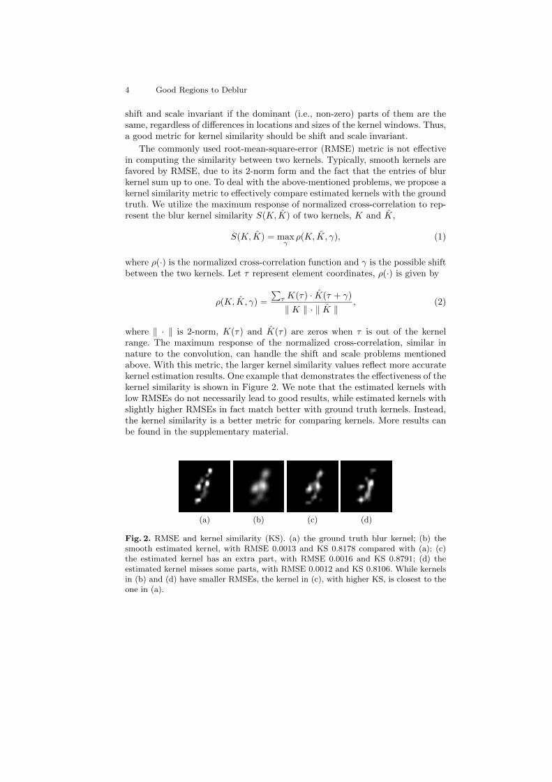
where ‖ · ‖ is 2-norm, K(τ) and K(τ) are zeros when τ is out of the kernelrange. The maximum response of the normalized cross-correlation, similar innature to the convolution, can handle the shift and scale problems mentionedabove. With this metric, the larger kernel similarity values reflect more accuratekernel estimation results. One example that demonstrates the effectiveness of thekernel similarity is shown in Figure 2. We note that the estimated kernels withlow RMSEs do not necessarily lead to good results, while estimated kernels withslightly higher RMSEs in fact match better with ground truth kernels. Instead,the kernel similarity is a better metric for comparing kernels. More results canbe found in the supplementary material.
(a) (b) (c) (d)
Fig. 2. RMSE and kernel similarity (KS). (a) the ground truth blur kernel; (b) thesmooth estimated kernel, with RMSE 0.0013 and KS 0.8178 compared with (a); (c)the estimated kernel has an extra part, with RMSE 0.0016 and KS 0.8791; (d) theestimated kernel misses some parts, with RMSE 0.0012 and KS 0.8106. While kernelsin (b) and (d) have smaller RMSEs, the kernel in (c), with higher KS, is closest to theone in (a).

Good Regions to Deblur 5
4 Learning Good Regions
Existing deblurring works discuss some potential features that may be useful forkernel estimation mainly based on empirical experimental results. In this paper,we address this problem by learning good image regions for deblurring.
4.1 Learning Framework
To determine the good image regions for deblurring, we analyze the image struc-ture by small subwindows. The subwindows within the image, in the context ofkernel estimation and recovered image, are spatially dependent. Two closelyoverlapping subwindows (e.g., shifted by a few pixels in either directions) sharesimilar image structures. In addition, it is reasonable to expect that other sub-windows, nearby a potential good subwindow for kernel estimation, contain use-ful image structures for deblurring. Consequently, the deblurred results for thesesubwindows should be similar, which are also observed empirically in image de-blurring results. Figure 3 shows one example where we estimate a blur kernelfrom each subwindow of size 200× 200 and apply it to recover the whole image.With all the estimated kernels from subwindows and recovered images, we con-struct an image reconstruction error map (Figure 3(b)) and a kernel similaritymap (Figure 3(c)) by comparing with ground truth clear image and blur kernel.The value at each pixel of these maps is computed by averaging the reconstruc-tion errors or kernel similarity values from all the subwindows containing it. Theimage reconstruction map illustrates that deblurred results using subwindowsfor kernel estimation are spatially correlated. In the meanwhile, high kernel sim-ilarity values well match low image reconstruction errors which demonstratesthe effectiveness of kernel similarity as a metric for evaluating deblurred results.Thus, we pose the problem of learning good regions within the CRF frame-work [6] as it encourages spatial correlation and label the training data usingkernel similarity.
(a) (b) (c)
Fig. 3. Spatial correlation. (a) input blurry image; (b) image reconstruction error mapbuilt upon the estimated kernels from shifting subwindows (blue to red pixels indicatelow to high reconstruction errors compared with the ground truth image); (c) kernelsimilarity map (blue to red pixels indicate high to low kernel similarity compared withthe ground truth kernel).

6 Good Regions to Deblur
Let S and i represent the set of nodes and node index. Given the labels yand the observations x, the conditional distribution P (y|x) is
P (y|x) =1
Zexp (E(y|x)) , (3)
where Z is a normalization term also known as the partition function. The energyE is
E(y|x) =∑i∈S
Ai(yi,x) +∑i∈S
∑j∈Ni
Iij(yi, yj ,x), (4)
where Ai and Iij denote the association and interaction potentials, respectively.The association potential Ai(yi,x) measures how likely the node of index iwould be labeled yi given the observation x. Meanwhile, the interaction po-tential Iij(yi, yj ,x) determines how the label yj at node j affects the one yi atnode i. Here Ni represents the neighborhood of node i.
In this paper, the subwindows in the input blurred image are considered asnodes in the CRF model similar to the formulation of discriminative randomfield [13]. Hence, we formulate association potential with log-likelihood of localdiscriminative model using the logistic function,
Ai(yi,x) = logP1(yi|hi(x))), (5)
where hi(·) denotes the feature vector of the local region at node i and the firstelement is set as 1 to accommodate the bias term. The conditional probabilityP1(yi|hi(x))) of class yi at node i is defined based on the logistic function:
P1(yi|hi(x)) = σ(yiw>hi(x)), (6)
where w are parameters of the logistic function σ.Similar to the association potential, the interaction potential is given by
I(yi, yj ,x) = logP2(yi, yj |µij(x)), (7)
andP2(yi, yj |µij(x)) = σ(yiyjv
>µij(x)), (8)
where v are the parameters of the logistic function and µij denotes the featurevector for pair (i, j). We adopt the difference of feature vector f between node iand j, with 1 as the first element, to express µij , µij(x) = [1, |hi(x)− hj(x)|]>.Since we do not encourage negative interaction for two nodes of different appear-ance or at image discontinuities, the term v>µij(x) is set to be non-negative.That is, we use the value max(0,v>µij(x)) to substitute v>µij(x).
4.2 Image Feature
Numerous prior works have shown that smooth image regions do not providesufficient information for kernel estimation, and instead textured regions areoften selected. Nevertheless, the estimation results may still be poor even whentextured regions are used [4]. Indeed, regions full of repetitive edges sometimesmake no contributions to the problem when the blur movement occurs in thesimilar direction as the edges (see an example in the supplementary material).
Good Regions to Deblur 7
To estimate blur kernels, recent algorithms focus on the use of sharp edges oredge distribution [3, 4]. Analogous to the problems with textured regions, sharpedges can be of great value for image deblurring under proper assumptions. Theunderlying assumption for effective use of sharp edges is that regions with highcontrast in the original image maintain informative structure after motion blur.However, not all the sharp edges are effective for kernel estimation. Recently, ithas been shown in [5] that edges of smaller size than the blur kernel may haveadverse effect on kernel estimation, and consequently edge maps of sufficient sizeare used for deblurring.
Taking all these factors into consideration, we present a method to extractfeatures from regions for image deblurring. We use the responses of a Gabor filterbank f(x) = [f1(x), f2(x), . . . , fn(x)] to represent the oriented textures of an im-age region x. Here n denotes the bin number of Gabor filters and fi(x) representsthe proportion that the i-th orientation is the dominant direction within the ob-servation x. The image gradient histogram g(x) = [hist(g1(x)),hist(g2(x))] isused to capture the distribution of edges, where g1 (x) and g2 (x) are the first-order derivatives of the image x along vertical and horizontal directions.
To rule out potential negative effects from small edges, we use the maskM(x) = H(r(x) − τ) as [5], where H(·) is the Heaviside step function whosevalue is zero for negative argument and otherwise one, and τ is the threshold.For each pixel p ∈ x, r(p) measures the usefulness of gradients by
r(p) =‖∑q∈Ns(p)
∇x(q) ‖∑q∈Ns(p)
‖ ∇x(q) ‖ +0.5, (9)
where Ns(p) is a s × s window centered at pixel p. The feature vector h(x) isthen formed by concatenating the above-mentioned local image features,
h(x) = [f(x), g(x), f(M(x)), g(M(x))], (10)
with varying parameters n, τ and s. We compare the proposed feature vectorswith some alternatives in the supplementary material.
4.3 Parameter Learning and Inference
Let θ denote the set of parameters in the CRF model, θ = {w,v}. The maximum-likelihood estimates of model parameters θ are computed with the pseudo-likelihood to approximate the partition function Z,
θ = arg maxθ
∏m
∏i∈Sm
P (ymi |xm,ymNi, θ), (11)
wherem represents the index of the training image and Sm is the graph generatedfrom the m-th image. Based on this formulation, we have
P (yi|x,yNi, θ) =
1
ziexp(Ai(yi,x) +
∑j∈Ni
I(yi, yj ,x)), (12)
and the partition function can be written as

8 Good Regions to Deblur
zi =∑
yi∈{−1,1}
exp(Ai(yi,x) +∑j∈Ni
I(yi, yj ,x)). (13)
To balance the effect between association and interaction potentials, we add inpenalty term 1
2φ2v>v, where the variable φ is pre-defined in this work. We solve
the optimization problem in the log pseudo-likelihood form,
θ = arg maxθ
∑m
∑i∈Sm
[log σ(yiw>hi(x))+
log∑j∈Ni
σ(yiyjv>µij(x))− log zi]−
1
2φ2v>v.
(14)
We use the BFGS method to solve the optimization problem and obtain param-eter θ. The loopy belief propagation (LBP) is then utilized for inference.
4.4 Good Regions to Deblur
Given a high resolution blurred image (e.g., 4000 × 3000 pixels), it is rathertime consuming to apply deblurring algorithms with the whole image. Evenwith the fast deblurring algorithm [14], it may not be the best choice to usethe whole image for kernel estimation for the reasons discussed in Section 4.2.We will demonstrate in Section 6 that using a region of blurred image for kernelestimation may render better deblurred result rather than using the whole image.Clearly, one immediate solution for these problems is to select a region within theinput image to estimate blur kernel, and then apply a non-blind deconvolutionalgorithm to the whole image.
In this work, we use principal component analysis to reduce the dimensional-ity of the feature vectors for learning the model parameters, and LBP to classifythe subwindows as good regions or not for blur kernel estimation. The label ofeach node (subwindow) in the training image is determined by comparing the es-timated kernel and the ground truth kernel. The learning process is summarizedin the supplementary material. The reason we use LBP for inference instead ofgraph cuts here is that we would like to obtain labels with confidence values sothat it is more convenient to develop a region selection strategy. We select thetop ranked subwindow to estimate kernel for simplicity although other weightedapproach may be used. Given the window size, the proposed method of selectinggood subwindow to deblur does not require manual selection which can be prob-lematic and time-consuming. We show that the proposed method can effectivelyselect the optimal subwindow for deblurring in Section 6.
Moreover, this window selection method can also be applied to non-uniform(spatially variant) blur cases which requires huge memory space and heavy com-putation if the whole image is used to estimate the camera motion (e.g., [14]).For instance, the non-uniform deblur algorithm [15] employs a RANSAC-basedscheme to select a set of patches for estimating local blur kernels and thus ren-dering a good initialization. With our method, it would be easy and effectiveto choose a set of good patches for local kernel estimation.
Good Regions to Deblur 9
5 Contribution of Feature Components
Within the model presented in Section 4, we use a feature vector consisting ofseveral components. In this section, we determine the most important componentfor image deblurring via their structured output. In addition, the approach weuse can also be extended to determine other effective features. We use a slightlydifferent energy function and consider each feature component independently.That is, we decompose the associate potential Ai(yi,x) into a combination offeature components:
Ai(yi|x) =∑c
αc logP c1 (yi|hci (x)), (15)
where hci represents different components of the feature vector, e.g., f(x) andf(M(x)), with weights α. The conditional probability P c1 (yi|hci (x)) is definedbased on the same logistic function as Eqn. 6. Since we aim to determinethe weights of feature components rather than the parameters of the logisticfunctions, the parameters of logistic functions are assumed to be known (e.g.,learned with a linear support vector machine). For interaction potential, we useI(yi, yj ,x) = βδ(yi − yj) to encourage labeling smoothness, where β > 0 is theweight and δ(·) denotes the Kronecker function.
The objective here is to maximize the probability of labels. In the trainingphase, we compute the weights Λ = (α, β) that assign the training labels ym
higher or equal probabilities than any other labels ym of training image m,
P (ym|xm) ≥ P (ym|xm),∀ym 6= ym. (16)
We can cancel the normalizer term Z from both sides of the constraints andexpress the constraints in terms of energies,
E(ym|xm) ≥ E(ym|xm),∀ym 6= ym. (17)
We take a max-margin approach to compute the weights that satisfy the in-equalities with the largest energy margin γ,
maxΛ:||Λ||=1
γ s. t. E(ym|xm)− E(ym|xm) ≥ γ,∀ym 6= ym. (18)
The weights Λ are constrained to have unity norm to prevent from growingwithout bound. Similar to [16], we learn the weights Λ by adding slack variablesand iteratively finding the minimum energy labeling with graph cuts [17]. Themain steps of this algorithm are summarized in the supplementary material.
6 Experimental Results
We evaluate the inferred subwindows using three state-of-the-art deblurring algo-rithms [2, 9, 14] and compare the performance using the error metric introducedin [1]. This metric computes the difference between a recovered image Ir and theknown ground-truth sharp image Ig, over the difference between the deblurredimage Ikg with the ground truth kernel kg and the ground-truth sharp image as||Ir − Ig||2/||Ikg − Ig||2. The cumulative histogram of reconstructed error ratio

10 Good Regions to Deblur
(briefed as cumulative error histogram for convenience) is then used to evaluatethe efficiency of an algorithm. Since the dataset from [1] has limited variabilityof image structure and blur kernel, we use the same technique to collect 400blurred image using 20 sharp images (with image size around 450× 450 pixels)and 20 blur kernels for training. These kernels are generated with different orien-tation and shape to simulate possible blur processes. Furthermore, we constructanother set of 120 challenging blurred images using 10 sharp images and 12 blurkernels for tests. Our experiments are carried out on a machine with 3.40 GHzCPU and 16 GB RAM. To infer an image of 450 × 450 pixels, it takes around5 seconds to process with our MATLAB implementation. The source codes anddata sets are available at http://faculty.ucmerced.edu/mhyang/code.
6.1 Deblurring with Good Regions
With the CRF model described in Section 4, we learn the parameters using allthe 400 training images for inferring good regions to deblur. For each image, webuild the graph model with overlapping subwindows of 200×200 pixels as nodesand shifts of 20 pixels. The size of subwindows is determined empirically as it islarge enough to estimate the kernel of size smaller than 29×29 pixels and all theblur kernels in this data set are like that. In our experiments, there are at least484 subwindows extracted from each image as the nodes for training. We collectthe estimated kernel from each subwindow using [2] as it is one of the best kernelestimators [1]. With the estimated kernels and ground truth kernels, we labelnode i to be 1 or −1 using the proposed kernel similarity S(Ki,K) between anestimated kernel Ki and the ground truth kernel K with the threshold λ of 0.6(empirically set for effectiveness), where Ki represents the estimated kernel fornode i. The feature parameters n, τ and s in this work are set to be 8, 0.6 to 0.9with increment of 0.1, and 9 to 24 with increment of 4 respectively. During theinference process, the size of subwindows is set proportional to the user-definedkernel size. That is, for a larger blur kernel, the size of subwindows selected toestimate the kernel should also be increased proportionally.
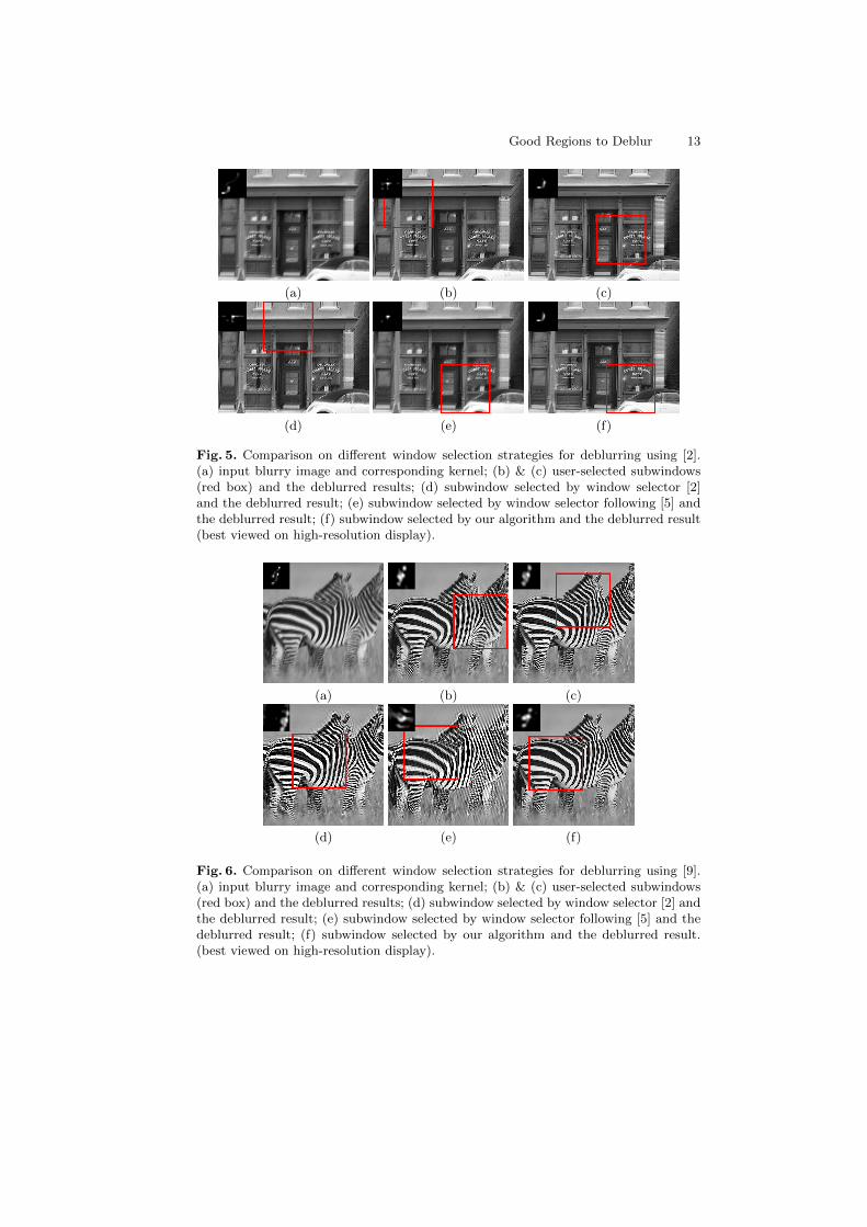
Comparison with User-selected Region To demonstrate that user selectioncan be replaced by our algorithm, we compare our top inferred subwindows withuser-selected regions. The users tend to choose regions with most salient edgesand variances as shown in Figure 5(b)(c) and Figure 6(b)(c). The user selectionstrategy works well in some situations but usually requires several trials to obtaina good result. On the contrary, our proposed method does not require userguidance and the deblurred results by the inferred subwindows of our algorithmoutperform that using user-selected regions.
Comparison with Region Selection Algorithms We compare the proposedalgorithm with two other region selection methods for deblurring [2, 5]. Theautomatic subwindow selector by [2] searches for the regions with high varianceand low saturation for kernel estimation. We implement another subwindowselection method by following the idea in [5] that the image deblurring processmay adversely degrade by the negative effect of small edges. In this selector, we

Good Regions to Deblur 11
remove small edges using the mask M(x) and then search for the subwindowwith most salient edges.
In this experiment, we select the top ranked subwindow from our inferencealgorithm for blur kernel estimation for simplicity although other alternativesmay be used. We apply other methods to select one subwindow from each imagefor kernel estimation and then apply two state-of-the-art algorithms [2, 9] torecover the whole image. Figure 5 and Figure 6 illustrate the comparison usingthe deblurring algorithm of [2] and [9] respectively. We note that although someinferred windows (e.g., Fig. 5(e) and (f)) appear to be similar, their locationsare different (60 pixels apart). The deblurring results on subwindows inferredby our algorithm are better than those from the other two subwindow selectionstrategies.
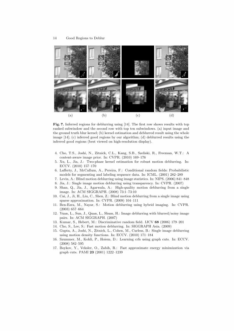
Comparison with Deblurring Using the Whole Image We also comparewith the deblurred results by [14] which uses the whole image for kernel esti-mation. In this experiment, we test two region selection strategies based on theinference results. One is to select the top ranked subwindow to estimate blurkernel, and another is to combine the top ten good subwindows. To combine thetop ten subwindows, we choose the smallest rectangle which covers all the sub-windows as the region for simplicity. We note that the top ranked subwindowsare usually clustered due to the usage of CRF model which encourages spa-tial correlation, and thus the rectangular region is still of small size comparedwith the whole image as shown in Figure 7. Compared to the results obtainedfrom the whole images in Figure 7, our algorithm with inferred region generatescomparable or superior kernel estimation and reconstructed images.
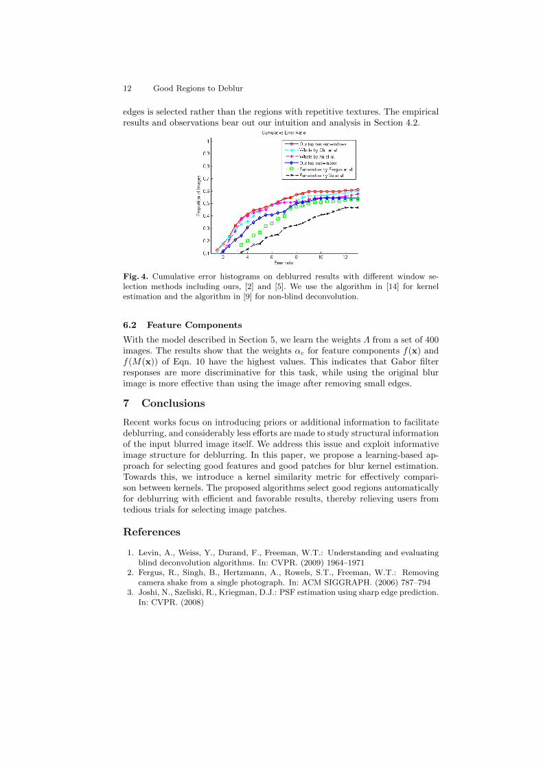
Quantitative Comparison We conduct extensive comparisons using 120 chal-lenging test images and present their cumulative error histograms. Given aninferred region by the proposed algorithm, we use the fast algorithm [14] to es-timate a blur kernel, and the non-blind deconvolution algorithm [9] to recoverthe latent image (similar as [14]). For thorough evaluations, we compare theresults using the above-mentioned region selection strategies [2] and the wholeimage [14]. In addition, we compare with [5] using a region or the whole image forkernel estimation. As shown in Figure 4, the curve using our top ten subwindowsgenerally performs better than other algorithms [14, 5] using the whole image.The results also show that not all the information in a blurred image is usefuland using the whole image for kernel estimation may not be the best choice. Wenote that the reconstructed results are visually plausible even when the errorratio is around 5 (an example is provided in the supplementary material), whichis different from the observations in [1]. The reason is that we employ differentnon-blind deconvolution algorithms and larger test images.
Analysis Our empirical results also provide some insights about the kinds ofimage structures that are favored by different deblurring algorithms. In the zebraimage, the selected window by our algorithm contains relatively strong edges, assuggested in [2, 1]. However, small or detailed edges may not help kernel estima-tion as shown in Figure 6(b). Furthermore, the subwindow with various oriented
12 Good Regions to Deblur
edges is selected rather than the regions with repetitive textures. The empiricalresults and observations bear out our intuition and analysis in Section 4.2.
Fig. 4. Cumulative error histograms on deblurred results with different window se-lection methods including ours, [2] and [5]. We use the algorithm in [14] for kernelestimation and the algorithm in [9] for non-blind deconvolution.
6.2 Feature Components
With the model described in Section 5, we learn the weights Λ from a set of 400images. The results show that the weights αc for feature components f(x) andf(M(x)) of Eqn. 10 have the highest values. This indicates that Gabor filterresponses are more discriminative for this task, while using the original blurimage is more effective than using the image after removing small edges.
7 Conclusions
Recent works focus on introducing priors or additional information to facilitatedeblurring, and considerably less efforts are made to study structural informationof the input blurred image itself. We address this issue and exploit informativeimage structure for deblurring. In this paper, we propose a learning-based ap-proach for selecting good features and good patches for blur kernel estimation.Towards this, we introduce a kernel similarity metric for effectively compari-son between kernels. The proposed algorithms select good regions automaticallyfor deblurring with efficient and favorable results, thereby relieving users fromtedious trials for selecting image patches.
References
1. Levin, A., Weiss, Y., Durand, F., Freeman, W.T.: Understanding and evaluatingblind deconvolution algorithms. In: CVPR. (2009) 1964–1971
2. Fergus, R., Singh, B., Hertzmann, A., Rowels, S.T., Freeman, W.T.: Removingcamera shake from a single photograph. In: ACM SIGGRAPH. (2006) 787–794
3. Joshi, N., Szeliski, R., Kriegman, D.J.: PSF estimation using sharp edge prediction.In: CVPR. (2008)
Good Regions to Deblur 13
(a) (b) (c)
(d) (e) (f)
Fig. 5. Comparison on different window selection strategies for deblurring using [2].(a) input blurry image and corresponding kernel; (b) & (c) user-selected subwindows(red box) and the deblurred results; (d) subwindow selected by window selector [2]and the deblurred result; (e) subwindow selected by window selector following [5] andthe deblurred result; (f) subwindow selected by our algorithm and the deblurred result(best viewed on high-resolution display).
(a) (b) (c)
(d) (e) (f)
Fig. 6. Comparison on different window selection strategies for deblurring using [9].(a) input blurry image and corresponding kernel; (b) & (c) user-selected subwindows(red box) and the deblurred results; (d) subwindow selected by window selector [2] andthe deblurred result; (e) subwindow selected by window selector following [5] and thedeblurred result; (f) subwindow selected by our algorithm and the deblurred result.(best viewed on high-resolution display).
14 Good Regions to Deblur
(a) (b) (c) (d)
Fig. 7. Inferred regions for deblurring using [14]. The first row shows results with topranked subwindow and the second row with top ten subwindows. (a) input image andthe ground truth blur kernel; (b) kernel estimation and deblurred result using the wholeimage [14]; (c) inferred good regions by our algorithm; (d) deblurred results using theinferred good regions (best viewed on high-resolution display).
4. Cho, T.S., Joshi, N., Zitnick, C.L., Kang, S.B., Szeliski, R., Freeman, W.T.: Acontent-aware image prior. In: CVPR. (2010) 169–176
5. Xu, L., Jia, J.: Two-phase kernel estimation for robust motion deblurring. In:ECCV. (2010) 157–170
6. Lafferty, J., McCallum, A., Pereira, F.: Conditional random fields: Probabilisticmodels for segmenting and labeling sequence data. In: ICML. (2001) 282–289
7. Levin, A.: Blind motion deblurring using image statistics. In: NIPS. (2006) 841–8488. Jia, J.: Single image motion deblurring using transparency. In: CVPR. (2007)9. Shan, Q., Jia, J., Agarwala, A.: High-quality motion deblurring from a single
image. In: ACM SIGGRAPH. (2008) 73:1–73:1010. Cai, J., Ji, H., Liu, C., Shen, Z.: Blind motion deblurring from a single image using
sparse approximation. In: CVPR. (2009) 104–11111. Ben-Ezra, M., Nayar, S.: Motion deblurring using hybrid imaging. In: CVPR.
(2003) 657–66412. Yuan, L., Sun, J., Quan, L., Shum, H.: Image deblurring with blurred/noisy image
pairs. In: ACM SIGGRAPH. (2007)13. Kumar, S., Hebert, M.: Discriminative random field. IJCV 68 (2006) 179–20114. Cho, S., Lee, S.: Fast motion deblurring. In: SIGGRAPH Asia. (2009)15. Gupta, A., Joshi, N., Zitnick, L., Cohen, M., Curless, B.: Single image deblurring
using motion density functions. In: ECCV. (2010) 171–18416. Szummer, M., Kohli, P., Hoiem, D.: Learning crfs using graph cuts. In: ECCV.
(2008) 582–59517. Boykov, Y., Veksler, O., Zabih, R.: Fast approximate energy minimization via
graph cuts. PAMI 23 (2001) 1222–1239