good practice guidance and uncertainty management...
TRANSCRIPT

Comprehensive list of the IPCC Publications
NGGIP Publications
Order Form
If you want to get copies inhardcover or CD-ROMs,please fill an order form andsend it to us. The order formcan be downloaded here.
Good Practice Guidance and Uncertainty Managementin
National Greenhouse Gas Inventories
This report on Good Practice Guidance andUncertainty Management in National Greenhouse GasInventories is the response to the request from theUnited Nations Framework Convention on ClimateChange (UNFCCC) for the Intergovernmental Panel onClimate Change (IPCC) to complete its work onuncertainty and prepare a report on good practice ininventory management.
This report provides good practice guidance to assistcountries in producing inventories that are neither overnor underestimates so far as can be judged, and inwhich uncertainties are reduced as far as practicable.
To this end, it supports the development of inventoriesthat are transparent, documented, consistent over time,complete, comparable, assessed for uncertainties,subject to quality control and quality assurance, andefficient in the use of resources.
This report does not revise or replace the Revised 1996 IPCC Guidelines for NationalGreenhouse Gas Inventories, but provides a reference that complements and is consistent withthose guidelines.
This report was accepted by the IPCC Plenary at its 16th session held in Montreal, 1-8 May,2000.
ContentsAcknowledgementPrefaceBasic Information
Chapter 1 IntroductionChapter 2 EnergyChapter 3 Industrial ProcessesChapter 4 AgricultureChapter 5 WasteChapter 6 Quantifying Uncertainties in PracticeChapter 7 Methodological Choice and RecalculationChapter 8 Quality Assurance and Quality ControlAnnex 1 Conceptual Basis for Uncertainty AnalysisAnnex 2 VerificationAnnex 3 GlossaryAnnex 4 List of Participants
Good Practice Guidance and Uncertainty Management
http://www.ipcc-nggip.iges.or.jp/public/gp/gpgaum.htm (1 of 2) [1/31/2001 2:32:46 PM]

IPCC National Greenhouse Gas Inventories ProgrammeTechnical Support Unit
C/o Institute for Global Environmental Strategies, 1560-39 Kamiyamaguchi, Hayama, Kanagawa, JAPAN 240-0198Phone: +81 468 55 3750 Fax: +81 468 55 3808
E-mail: [email protected]: http://www.ipcc-nggip.iges.or.jp
INTERGOVERNMENTAL PANEL ON CLIMATE CHANGEWMO UNEPNATIONAL GREENHOUSE GAS INVENTORIES PROGRAMME
Order Form September 2000
Please return this form to: Technical Support UnitIPCC NGGIPC/o Institute for Global Environmental Strategies1560-39 Kamiyamaguchi, HayamaKanagawa 240-0198 JapanFax: +81 468 55 [email protected]
Good Practice Guidance and Uncertainty Management inNational Greenhouse Gas InventoriesPlease send copies in hardcover @ J ¥ 4900 ¥
(Approximately US $45)Please send copies of CD-ROM @ J ¥ 700 ¥
(Approximately US $6) *Revised 1996 IPCC Guidelines for National Greenhouse Gas Inventories are also included in the CD-ROM.
Shipping/mailing and Handling Charges : Add the shipping/mailing cost per order. No handling charge.
Order from developing countries and EIT: IPCC will cover costs for Developing and EIT countries
Ship to :Name:
Institution:
Address:
City: State/Province/Prefecture
Postcode: Country:
Tel: Fax:
E-mail:
□□□□ Surface Express Mail □□□□ Air Mail □□□□ Business Express Mail
Payment :□□□□Charge my credit Card: □□□□ Visa □□□□ Master Card □□□□ American Express □□□□ JCB
Card Number:
Please note that the total amount charged for the purchase may differ from the quoted price becauseall currencies including US dollars will be converted to Japanese Yen.
Expiry Date: Signature:
Name of Cardholder:
□□□□ Money transfer to: Sakura Bank Ltd.Branch: Head OfficeAccount Name: Institute for Global Environmental Strategies IPCC-TSUAccount Number: 084-3022167Re: IPCC Report on Good Practice Guidance
Orders will be held for 2 weeks or until money transfer is completed.Price may be changed without notice.

Table of Contents
IPCC Good Practice Guidance and Uncertainty Management in National Greenhouse Gas Inventories
C O N T E N T S
ACKNOWLEDGEMENT ....................................................................................................................................... iv
PREFACE ................................................................................................................................................................v
Basic Information ................................................................................................................................................. vii
CHAPTERS
1 Introduction .................................................................................................................................................. 1.1
2 Energy .......................................................................................................................................................... 2.1
3 Industrial Processes ...................................................................................................................................... 3.1
4 Agriculture ................................................................................................................................................... 4.1
5 Waste ............................................................................................................................................................ 5.1
6 Quantifying Uncertainties in Practice .......................................................................................................... 6.1
7 Methodological Choice and Recalculation ................................................................................................... 7.1
8 Quality Assurance and Quality Control ....................................................................................................... 8.1
ANNEXES
Annex 1 Conceptual Basis for Uncertainty Analysis .................................................................................. A1.1
Annex 2 Verification ................................................................................................................................... A2.1
Annex 3 Glossary ........................................................................................................................................ A3.1
Annex 4 List of Participants ........................................................................................................................ A4.1
Acknowledgement
IPCC Good Practice Guidance and Uncertainty Management in National Greenhouse Gas Inventoriesiv
ACKNOWLEDGEMENT
The overall chair for this project on Good Practice Guidance and Uncertainty Management in NationalGreenhouse Gas Inventories was Jim Penman (UK). Dina Kruger (USA) and Ian Galbally (AUS) were co-chairsof the development of the sectoral ‘Good Practice Guidance’ and ‘Uncertainty Management’ respectively.
The co-chairs of the source/subject level expert groups provided their time and expertise along with otherexperts, from a wide range of disciplines, who also gave of their time to write, comment and review the text andattend meetings. Expert meetings were held in Australia (Finalisation), Brazil (Waste), Czech Republic (Energy),France (Scoping), Netherlands (Agriculture), United Kingdom (Uncertainty) and the USA (Industrial Processes).Financial and in kind contributions were received from governments.
Technical and organisational support for the project was provided by the IPCC/OECD/IEA Secretariat in Paristhat oversaw the initiation of the project and sectoral good practice development. Thomas Martinsen was theProgramme Manager. Katarina Mareckova, Robert Hoppaus and Pierre Boileau were the Programme Officerswith Amy Emmert as Secretary.
The Technical Support Unit (TSU) of the IPCC National Greenhouse Gas Inventories Programme that took overfrom the Secretariat in Paris is located in the Institute for Global Environmental Strategies and funded by theGovernment of Japan. Sal Emmanuel is the Head of the Unit. The four Programme Officers are LeandroBuendia, Robert Hoppaus, Jeroen Meijer and Kiyoto Tanabe. Kyoko Miwa is the Administrative Officer andMakiko Ishikawa looked after Secretarial activities. Kyoko Takada is the current Secretary. Bill Irving (USEPA)worked extensively on the text.
Taka Hiraishi (Japan) and Buruhani Nyenzi (Tanzania), the two co-chairs of the Task Force Bureau for the IPCCNational Greenhouse Gas Inventories Programme and their colleagues, the Task Force Bureau membersprovided guidance, encouragement and input to the process.
Bob Watson, Chairman of the IPCC and Narasimhan Sundararaman, IPCC Secretary both provided support,advice and encouragement. Assistance for the project was also provided by the IPCC Secretariat, RudieBourgeois, Annie Courcin and Chantal Ettori.
IPCC
Robert Watson, ChairNarasimhan Sundararaman, Secretary
IPCC NGGIP Task Force Bureau
Taka Hiraishi, co-chairBuruhani Nyenzi, co-chairIan CarruthersMarc GilletDina KrugerCarlos LopezLeo MeyerDomingos MiguezWang MinxingIgor NazarovRichard OdingoRajendra PachauriJim PenmanAudun RoslandJohn Stone
IPCC NGGIP JapanTechnical Support Unit
Sal EmmanuelLeandro BuendiaRobert HoppausJeroen MeijerKyoko MiwaKiyoto TanabeKyoko Takada

Preface
IPCC Good Practice Guidance and Uncertainty Management in National Greenhouse Gas Inventories v
PREFACE1
This report on Good Practice Guidance and Uncertainty Management in National Greenhouse Gas Inventories(Good Practice Report) is the response to the request from the United Nations Framework Convention onClimate Change (UNFCCC) for the Intergovernmental Panel on Climate Change (IPCC) to complete its work onuncertainty and prepare a report on good practice in inventory management.
The Good Practice Report provides good practice guidance to assist countries in producing inventories that areneither over nor underestimates so far as can be judged, and in which uncertainties are reduced as far aspracticable.
To this end, it supports the development of inventories that are transparent, documented, consistent over time,complete, comparable, assessed for uncertainties, subject to quality control and quality assurance, and efficientin the use of resources.
The Good Practice Report treats four main topics. Firstly, Chapters 2-5 contain good practice guidanceaddressing the Energy, Industrial Processes, Agriculture, and Waste Sectors. These chapters address:
• Choice, by means of decision trees, of estimation methods suited to national circumstances;
• Advice on the most suitable emission factors and other data necessary for inventory calculations;
• Quality assurance and quality control procedures to enable cross-checks during inventory compilation;
• Information to be documented, archived and reported to facilitate review of emission estimates;
• Uncertainties at the source category level.
Secondly, Chapter 6, Quantifying Uncertainties in Practice, describes how to determine the relative contributionthat each source category makes to the overall uncertainty of national inventory estimates, using a combinationof empirical data and expert judgement. The chapter describes methods that will help inventory agencies reporton uncertainties in a consistent manner, and provides input to national inventory research and developmentactivities.Thirdly, since inventory development is resource-intensive, and estimates are likely to improve in the future,Chapter 7, Methodological Choice and Recalculation, provides guidance on how to prioritise key sourcecategories, and also shows how and when to recalculate previously prepared emission estimates to ensureconsistent estimation of trends.Finally, Chapter 8, Quality Assurance and Quality Control, describes good practice in quality assurance andquality control procedures for inventory agencies with respect to their own inventories. Good practice guidancecovers measurement standards, routine computational and completeness checks, and documentation and dataarchiving procedures. A system of independent review and auditing is also described.
Three annexes provide supporting material on basic concepts, definitions and verification.
The Good Practice Report does not revise or replace the IPCC Guidelines2, but provides a reference thatcomplements and is consistent with those guidelines. Consistency with the IPCC Guidelines is defined by threecriteria:
(i) Specific source categories addressed by good practice guidance have the same definitions as thecorresponding categories in the IPCC Guidelines.
(ii) Good practice guidance uses the same functional forms for the equations used to estimateemissions that are used in the IPCC Guidelines.
(iii) Good practice guidance allows the correction of errors or deficiencies that have been identified inthe IPCC Guidelines.
Criterion (i) does not exclude the identification of additional source categories that may be included in the Othercategory in the IPCC Guidelines. Default emission factors or model parameter values have been updated, wherethey can be linked to particular national circumstances, and documented.
1 Preface agreed by the Task Force Bureau for the IPCC National Greenhouse Gas Inventories Programme that met inSydney on 4 March 2000.
2 Full title: Revised 1996 IPCC Guidelines for National Greenhouse Gas Inventories (IPCC, 1996).

Preface
vi IPCC Good Practice Guidance and Uncertainty Management in National Greenhouse Gas Inventories
Whatever the level of complexity of the inventory, good practice guidance provides improved understanding ofhow uncertainties may be managed to produce emissions estimates suitable for the purposes of the UNFCCC andfor the scientific work associated with greenhouse gas inventories.

Basic information
IPCC Good Practice Guidance and Uncertainty Management in National Greenhouse Gas Inventories vii
BASIC INFORMATION
Prefixes and multiplication factorsMultiplication Factor Abbreviation Prefix Symbol
1 000 000 000 000 000 1015 peta P
1 000 000 000 000 1012 tera T
1 000 000 000 109 giga G
1 000 000 106 mega M
1 000 103 kilo k
100 102 hecto h
10 101 deca da
0.1 10-1 deci d
0.01 10-2 centi c
0.001 10-3 milli m
0.000 001 10-6 micro µ
Abbreviations for chemical compoundsCH4 Methane
N2O Nitrous oxide
CO2 Carbon dioxide
CO Carbon monoxide
NOX Nitrogen oxides
NMVOC Non-methane volatile organic compound
NH3 Ammonia
CFCs Chlorofluorocarbons
HFCs Hydrofluorocarbons
PFCs Perfluorocarbons
SF6 Sulfer hexafluoride
CCl4 Carbon tetrachloride
C2F6 Hexafluoroethane
CF4 Tetrafluoromethane

Basic information
viii IPCC Good Practice Guidance and Uncertainty Management in National Greenhouse Gas Inventories
Standard equivalents1 tonne of oil equivalent (toe) 1 x 10¹⁰ calories
103 toe 41.868 TJ
1 short ton 0.9072 tonne
1 tonne 1.1023 short tons
1 tonne 1 megagram
1 kilotonne 1 gigagram
1 megatonne 1 teragram
1 gigatonne 1 petagram
1 kilogram 2.2046 lbs
1 hectare 104 m2
1 calorieIT 4.1868 Joules
1 atmosphere 101.325 kPa
Units1 and abbreviationscubic metre m3
hectare ha
gram g
tonne t
joule J
degree Celsius ℃
calorie cal
year yr
capita cap
gallon gal
dry matter dm
1 For decimal prefixes see previous page.

Chapter 1 Introduction
IPCC Good Practice Guidance and Uncertainty Management in National Greenhouse Gas Inventories 1.1
1
INTRODUCTION
Introduction Chapter 1
1.2 IPCC Good Practice Guidance and Uncertainty Management in National Greenhouse Gas Inventories
C o n t e n t s
1 INTRODUCTION
1.1 DEVELOPMENT OF THE PROGRAMME ........................................................................................1.3
1.2 QUANTIFYING UNCERTAINTIES IN ANNUAL INVENTORIES AND TRENDS .......................1.3
1.3 ROLE OF GOOD PRACTICE IN MANAGING UNCERTAINTIES .................................................1.4
1.4 POLICY RELEVANCE........................................................................................................................1.6
F i g u r e
Figure 1.1 Example-Decision Tree for CH4 Emissions from Solid Waste Disposal Sites ................1.5

Chapter 1 Introduction
IPCC Good Practice Guidance and Uncertainty Management in National Greenhouse Gas Inventories 1.3
1 INTRODUCTION
1 . 1 D E V E L OP ME N T OF T HE P R OGR A M M EAt its 8th session in June 1998, the Subsidiary Body for Scientific and Technological Advice (SBSTA-8) of theUnited Nations Framework Convention on Climate Change (UNFCCC), encouraged the IPCC-OECD-IEAInventories Programme to give high priority to completing its work on uncertainty, as well as to prepare areport on good practices in inventory management and to submit a report on these issues for consideration bythe SBSTA, if possible by COP5. This report is the IPCC’s (Intergovernmental Panel on Climate Change)response to the SBSTA.
To prepare for the work required, the IPCC held an Expert Meeting in Paris in October 1998. The Paris meetingtreated good practice as a way to manage uncertainties, as these would remain associated with greenhouse gasemissions inventories for the foreseeable future. Good practice guidance assists countries in producinginventories that are accurate in the sense of being neither over nor underestimates so far as can be judged, and inwhich uncertainties are reduced as far as practicable. Good practice guidance further supports the developmentof inventories that are transparent, documented, consistent over time, complete, comparable, assessed foruncertainties, subject to quality control and assurance, efficient in the use of the resources available to inventoryagencies, and in which uncertainties are gradually reduced as better information becomes available.
The Paris meeting planned a series of four sectoral Expert Meetings to define good practice by sector and sourcecategory. These meetings covered, respectively, (i) industrial process emissions1 and emissions of newgreenhouse gases i.e., hydrofluorocarbons (HFCs), perfluorocarbons (PFCs), and sulphur hexafluoride (SF6), (ii)emissions associated with energy production and consumption, (iii) agricultural emissions and (iv) emissionsfrom waste.
The four sectoral meetings were followed by a meeting on quantifying uncertainties and cross-cutting issues ininventory management, and a concluding meeting to finalise the work. Emissions and removals associated withcarbon stocks in land use, land-use change and forestry were not addressed in this phase of work because of theparallel IPCC activity to produce a Special Report on this Sector. The Paris meeting anticipated the need todefine good practice in this area also, once the Special Report is complete and the Parties have had time toconsider it. Currently, good practice guidance covers emissions of the direct greenhouse gases: carbon dioxide(CO2), methane (CH4), nitrous oxide (N2O), HFCs, PFCs, and SF6. Emissions of the precursor gases carbonmonoxide (CO), nitrogen oxides (NOx), and non-methane volatile organic compounds (NMVOCs) were notcovered in this phase of good practice but could form part of the future work programme. Emissions associatedwith Solvents and Other Product Use are not covered in this report as the main gases emitted in this sector fallinto the class of NMVOCs.
It soon became clear that the programme initiated in Paris could not be completed by the fifth Conference of theParties to the UNFCCC (COP5), especially given the need for the report to go through the process ofgovernment and expert review. Also, with regard to the UNFCCC, the timetable for methodological work agreedat COP4 required substantive outputs by COP6. Therefore, the timetable was extended, so that the IPCC’s reporton Good Practice Guidance and Uncertainty Management in National Greenhouse Gas Inventories could beavailable to the Parties at COP6 rather than COP5.
1 . 2 QU A N T I F Y I N G U N C E R T A I N T I E S I NA N N U A L I N V E N T O R I E S A N D T R E N D S
The IPCC Guidelines contain some quantitative advice on uncertainties,2 although so far relatively few countrieshave reported on uncertainties in a systematic way.
1 Good practice guidance complementary to the IPCC Guidelines has not been developed for some categories of industrialemissions that are identified at the beginning of Chapter 3, Industrial Processes.
2 Revised 1996 IPCC Guidelines for National Greenhouse Gas Inventories, Vol. 1, Annex 1, Managing Uncertainties (IPCC,1996).

Introduction Chapter 1
1.4 IPCC Good Practice Guidance and Uncertainty Management in National Greenhouse Gas Inventories
Nevertheless, evidence considered by the Paris meeting indicated that for a developed country the overalluncertainty in emissions weighted by global warming potentials (GWPs) in a single year could be of the order of20%, mainly due to uncertainties in non-CO2 gases.3
Analysis also indicated that the uncertainty in the trend in emissions may be less than the uncertainty in theabsolute value of emissions in any year. This is because a method that over or underestimates emissions from asource category in one year may similarly over or underestimate emissions in subsequent years. The preliminaryevidence available to the Paris meeting suggested that, when this compensation is taken into account, theuncertainty on the trend in emissions between years could fall to a few percent for industrialised countries.4
Chapter 6, Quantifying Uncertainties in Practice, of this report describes methods to determine the uncertainty ineach source category. These methods use a combination of empirical data and expert judgement according toavailability. They estimate the relative contribution that the source category makes to the overall uncertainty ofnational inventory estimates, in terms of the trend as well as absolute level. These methods are consistent withthe conceptual guidance on uncertainties in Annex 1, Conceptual Basis for Uncertainty Analysis. They willenable countries to report on uncertainties in a consistent manner, and provide valuable input to nationalinventory research and development activities. The methods are capable of allowing for relationships inuncertainties between different inventory components, and are supplemented by an extensive set of defaultuncertainties developed through the sector workshops.
1 . 3 R O L E O F G O O D P R A C T I C E I NM A N A G I N G U N C E R T AI N T IE S
To be consistent with good practice as defined in this report, inventories should contain neither over norunderestimates so far as can be judged, and the uncertainties in these estimates should be reduced as far aspractible.
These requirements are to ensure that emissions estimates, even if uncertain, are bona fide estimates, in the senseof not containing any biases that could have been identified and eliminated, and that uncertainties have beenminimised as far as practible given national circumstances. Estimates of this type would presumably be the bestattainable, given current scientific knowledge and available resources.
Good practice aims to deliver these requirements by providing guidance on:
• Choice of estimation method within the context of the IPCC Guidelines;
• Quality assurance and quality control procedures to provide cross-checks during inventory compilation;
• Data and information to be documented, archived and reported to facilitate review and assessment ofemission estimates;
• Quantification of uncertainties at the source category level and for the inventory as a whole, so that theresources available for research can be directed toward reducing uncertainties over time, and theimprovement can be tracked.
Chapters 2 to 5 set out good practice guidance on the choice of estimation method at the source category levelby means of decision trees of the type illustrated in Figure 1.1, Example-Decision Tree for CH4 Emissions fromSolid Waste Disposal Sites. The decision trees formalise the choice of the estimation method most suited tonational circumstances. The source category guidance linked to the decision trees also provides information onthe choice of emission factors and activity data, and on the associated uncertainty ranges needed to support theuncertainty estimation procedures described in Chapter 6, Quantifying Uncertainties in Practice. The mostappropriate choice of estimation method (or tier) will depend on national circumstances, including theavailability of resources and can be determined according to the methods set out in Chapter 7, MethodologicalChoice and Recalculation.
Inventory development is a resource intensive enterprise which means firstly that inventory agencies may needto prioritise among source categories and estimation methods, and secondly that data quality may improve overtime. Guidance applicable to all source categories is given in Chapter 7, regarding how to identify the key source
3 Based on an analysis of the UK inventory presented to the Paris meeting (Eggleston et al., 1998) and which is described inmore detail in Chapter 6, Quantifying Uncertainties in Practice, Section 6.3.1, Comparison between Tiers and Choice ofMethod.
4 See footnote 3

Chapter 1 Introduction
IPCC Good Practice Guidance and Uncertainty Management in National Greenhouse Gas Inventories 1.5
categories that should be prioritised in the inventory development process, as well as when and how torecalculate previously prepared emissions estimates to ensure consistent emission trends. A key source categoryis defined in Chapter 7, as one that has a significant influence on a country’s total inventory of direct greenhousegases in terms of the absolute level of emissions or the trend, or both. The outcome of the determination of thekey source category analysis is taken into account during inventory preparation as indicated in the decision trees.Chapter 7, also addresses means to manage methodological changes and recalculations. For example, a change ina method may be due to the introduction of emissions’ abatement technology, the availability of more detaileddata, or the greater significance of a source category whose rapid variation over time substantially affects thetrend in total emissions. Guidance is provided for splicing time series in those cases where changes in methodsare consistent with good practice.
Good practice in quality assurance and quality control (QA/QC) procedures described in Chapter 8, QualityAssurance and Quality Control, covers measurement standards, routine computational and completeness checks,and documentation and data archiving procedures to be applied to the inventory at the compilation stage. Chapter8, also describes a system of independent review and auditing that could be implemented by inventory agencies.QA/QC as defined here covers only actions that inventory agencies could take in respect of their owninventories. It does not include an international system of review, except insofar as the requirements fortransparency would be common between an international review process and internal reviews conductedroutinely by inventory agencies.
F i g u r e 1 . 1 E x a m p l e - D e c i s i o n T r e e f o r C H 4 E m i s s i o n s f r o m S o l i dW a s t e D i s p o s a l S i t e s
Throughout this report, good practice refers to actions that could be undertaken by inventory agencies inproducing their greenhouse gas inventories. However, the request from the SBSTA is not restricted to nationalactions, and in the Annexes the report reflects the broader picture, both scientifically and internationally.
Box 1
No
Box 2
No
Yes
Are wastedisposal activity
data obtainable for thecurrent inventory
year?
Use IPCC defaultvalues, per capita or
other methods toestimate activity data
Estimate CH4emissions using the
IPCC defaultmethod
Are wastedisposal activity dataavailable for previous
years?
Is this akey source category?
(Note 1)
Estimate CH4emissions using theFirst Order Decay
(FOD) method
Obtain orestimate data on
historical changes insolid waste disposal
Yes
No
Yes
Note 1: A key source category is one that is prioritised within the national inventory system because its estimate has a significantinfluence on a country’s total inventory of direct greenhouse gases in terms of the absolute level of emissions, the trend in emissions, orboth. (See Chapter 7, Methodological Choice and Recalculation, Section 7.2, Determining National Key Source Categories.)
Introduction Chapter 1
1.6 IPCC Good Practice Guidance and Uncertainty Management in National Greenhouse Gas Inventories
Annex 1, Conceptual Basis for Uncertainty Analysis, deals with the concepts that underlie the practical adviceon uncertainties provided in Chapters 2 to 8 of the main report. Annex 2, Verification, discusses internationaland scientific aspects of inventory verification. Annex 3, the Glossary, defines the terms of particular interest inthe context of greenhouse gas inventories, and also summarises mathematical definitions of selected statisticalterms for convenient reference.
1 . 4 P O L I C Y R E L E V A N C EThe report on Good Practice Guidance and Uncertainty Management in National Greenhouse Gas Inventories(Good Practice Report) does not revise or replace the IPCC Guidelines, but provides a reference thatcomplements and is consistent with these Guidelines. This is because the Conference of the Parties decided5 thatthese IPCC Guidelines would be used for reporting by Parties included in Annex I to the UNFCCC. For thepurposes of developing good practice guidance, consistency with the IPCC Guidelines is defined by threecriteria:
(i) Specific source categories addressed by good practice guidance have the same definitions as thecorresponding categories in the IPCC Guidelines.
(ii) Good practice guidance uses the same functional forms for the equations used to estimateemissions that are used in the IPCC Guidelines.
(iii) Good practice guidance allows correction of any errors or deficiencies6 that have been identified inthe IPCC Guidelines.
Criterion (i) does not exclude identification of additional source categories that may be included in the Othercategory in the IPCC Guidelines. Default emission factors or model parameter values have been updated wherethey can be linked to particular national circumstances and documented.
The main development in the negotiations since the SBSTA-8’s request has been agreement on the revisedreporting guidelines for Annex I Parties’ greenhouse gas inventories.7 These UNFCCC guidelines contain crossreferences to the IPCC’s work on good practice concerning choice of methodology, emission factors, activitydata, uncertainties, quality assessment and quality control procedures, time series consistency, accuracy andverification.
It is through good practice guidance and uncertainty management that a sound basis can be provided to producemore reliable estimates of the magnitude of absolute and trend uncertainties in greenhouse gas inventories thanhas been achieved previously. Whatever the level of complexity of the inventory, good practice providesimproved understanding of how uncertainties may be managed to produce emissions estimates that areacceptable for the purposes of the UNFCCC, and for the scientific work associated with greenhouse gasinventories.
5 Decision 2/CP.3 and the document FCCC/CP/1999/7 referred to in decision 3/CP.5.
6 For example, some of the equations in the IPCC Guidelines do not formally allow for emissions mitigation technologies ortechniques.
7 See Decision 3/CP.5.

Chapter 2 Energy
IPCC Good Practice Guidance and Uncertainty Management in National Greenhouse Gas Inventories 2.1
2
ENERGY

Energy Chapter 2
2.2 IPCC Good Practice Guidance and Uncertainty Management in National Greenhouse Gas Inventories
CO-CHAIRS, EDITORS AND EXPERTS
Co-chairs of the Expert Meeting on Emissions from EnergyTaka Hiraishi (Japan) and Buruhani Nyenzi (Tanzania)
REVIEW EDITOR
Marc Gillet (France)
AUTHORS OF GENERAL BACKGROUND PAPER
Jeroen Meijer (IEA) and Tinus Pullus (Netherlands)
Expert Group: CO2 Emissions from Stationary CombustionCO-CHAIRS
Tim Simmons (UK) and Milos Tichy (Czech Republic)
AUTHOR OF BACKGROUND PAPER
Tim Simmons (UK)
CONTRIBUTORS
Agus Cahyono Adi (Indonesia), Monika Chandra (USA), Sal Emmanuel (Australia), Jean-Pierre Fontelle(France), Pavel Fott (Czech Republic), Kari Gronfors (Finland), Dietmar Koch (Germany), Wilfred Kipondya(Tanzania), Sergio Lamotta (Italy), Elliott Lieberman (USA), Katarina Mareckova (IPCC/OECD), RobertoAcosta (UNFCCC secretariat), Newton Paciornik (Brazil), Tinus Pulles (Netherlands), Erik Rassmussen(Denmark), Sara Ribacke (Sweden), Bojan Rode (Slovenia), Arthur Rypinski (USA), Karen Treanton (IEA), andStephane Willems (OECD)
Expert Group: Non-CO2 Emissions from Stationary CombustionCO-CHAIRS
Samir Amous (Tunisia) and Astrid Olsson (Sweden)
AUTHOR OF BACKGROUND PAPER
Samir Amous (Tunisia)
CONTRIBUTORS
Ijaz Hossain (Bangladesh), Dario Gomez (Argentina), Markvart Miroslav (Czech Republic), Jeroen Meijer(IEA), Michiro Oi (Japan), Uma Rajarathnam (India), Sami Tuhkanen (Finland), and Jim Zhang (USA)
Expert Group: Mobile Combustion: Road TransportCO-CHAIRS
Michael Walsh (USA) and Samir Mowafy (Egypt)
AUTHOR OF BACKGROUND PAPER
Simon Eggleston (UK)
CONTRIBUTORS
Javier Hanna (Bolivia), Frank Neitzert (Canada), Anke Herold (Germany), Taka Hiraishi (Japan), BuruhaniNyenzi (Tanzania), Nejib Osman (Tunisia), Simon Eggleston (UK), David Greene (UK), Cindy Jacobs (USA),and Jean Brennan (USA)

Chapter 2 Energy
IPCC Good Practice Guidance and Uncertainty Management in National Greenhouse Gas Inventories 2.3
Expert Group: Mobile Combustion: Water-borne NavigationCHAIR
Wiley Barbour (USA)
AUTHORS OF BACKGROUND PAPER
Wiley Barbour, Michael Gillenwater, Paul Jun
CONTRIBUTORS
Leonnie Dobbie (Switzerland), Robert Falk (UK), Michael Gillenwater (USA), Robert Hoppaus (IPCC/OECD),Roberto Acosta (UNFCCC secretariat), Gilian Reynolds (UK), and Kristin Rypdal (Norway)
Expert Group: Mobile Combustion: AviationCHAIR
Kristin Rypdal (Norway)
AUTHOR OF BACKGROUND PAPER
Kristin Rypdal (Norway)
CONTRIBUTORS
Wiley Barbour (USA), Leonie Dobbie (IATA), Robert Falk (UK), Michael Gillenwater (USA), and RobertHoppaus (IPCC/OECD)
Expert Group: Fugitive Emissions from Coal Mining and HandlingCO-CHAIRS
David Williams (Australia) and Oleg Tailakov (Russia)
AUTHORS OF BACKGROUND PAPER
William Irving (USA) and Oleg Tailakov (Russia)
CONTRIBUTORS
William Irving (USA) and Huang Shenchu (China)
Expert Group: Fugitive Emissions from Oil and Natural Gas ActivitiesCO-CHAIRS
David Picard (Canada) and Jose Domingos Miguez (Brazil)
AUTHOR OF BACKGROUND PAPER
David Picard (Canada)
CONTRIBUTORS
Marc Darras (France), Eilev Gjerald (Norway), Dina Kruger (USA), Robert Lott (USA), Katarina Mareckova(IPCC/OECD), Marc Phillips (USA), and Jan Spakman (Netherlands)

Energy Chapter 2
2.4 IPCC Good Practice Guidance and Uncertainty Management in National Greenhouse Gas Inventories
C o n t e n t s
2 ENERGY
2.1 CO2 EMISSIONS FROM STATIONARY COMBUSTION ................................................................2.8
2.1.1 Methodological issues ...............................................................................................................2.8
2.1.2 Reporting and documentation ..................................................................................................2.15
2.1.3 Inventory quality assurance/quality control (QA/QC) .............................................................2.16
Appendix 2.1A.1 Reporting of emissions of fossil carbon-based moleculesaccording to the Revised 1996 IPCC Guidelines source categories ....................2.18
Appendix 2.1A.2 Method to estimate carbon content based on API gravity and sulfur content ......2.19
Appendix 2.1A.3 1990 country-specific net calorific values ...........................................................2.25
2.2 NON-CO2 EMISSIONS FROM STATIONARY COMBUSTION.....................................................2.37
2.2.1 Methodological issues .............................................................................................................2.37
2.2.2 Reporting and documentation ..................................................................................................2.42
2.2.3 Inventory quality assurance/quality control (QA/QC) .............................................................2.42
2.3 MOBILE COMBUSTION: ROAD VEHICLES .................................................................................2.44
2.3.1 Methodological issues .............................................................................................................2.44
2.3.2 Reporting and documentation ..................................................................................................2.49
2.3.3 Inventory quality assurance/quality control (QA/QC) .............................................................2.49
2.4 MOBILE COMBUSTION: WATER-BORNE NAVIGATION .........................................................2.51
2.4.1 Methodological issues .............................................................................................................2.51
2.4.2 Reporting and documentation ..................................................................................................2.55
2.4.3 Inventory quality assurance/quality control (QA/QC) .............................................................2.56
2.5 MOBILE COMBUSTION: AIRCRAFT.............................................................................................2.57
2.5.1 Methodological issues .............................................................................................................2.57
2.5.2 Reporting and documentation ..................................................................................................2.63
2.5.3 Inventory quality assurance/quality control (QA/QC) .............................................................2.64
Appendix 2.5A.1 Fuel use and average sector distance for representative types of aircraft.............2.65
Appendix 2.5A.2 Correspondence between representative aircraft and other aircraft types ............2.67
Appendix 2.5A.3 Fuel consumption factors for military aircraft......................................................2.69
2.6 FUGITIVE EMISSIONS FROM COAL MINING AND HANDLING..............................................2.70
2.6.1 Methodological issues .............................................................................................................2.70
2.6.2 Reporting and documentation ..................................................................................................2.77
2.6.3 Inventory quality assurance/quality control (QA/QC) .............................................................2.78
2.7 FUGITIVE EMISSIONS FROM OIL AND GAS OPERATIONS.....................................................2.79
2.7.1 Methodological issues .............................................................................................................2.79
2.7.2 Reporting and documentation ..................................................................................................2.92
2.7.3 Inventory quality assurance/quality control (QA/QC) .............................................................2.93

Chapter 2 Energy
IPCC Good Practice Guidance and Uncertainty Management in National Greenhouse Gas Inventories 2.5
REFERENCES ............................................................................................................................................2.94
Energy Chapter 2
2.6 IPCC Good Practice Guidance and Uncertainty Management in National Greenhouse Gas Inventories
F i g u r e s
Figure 2.1 Decision Tree for Selecting the Method for Estimation of CO2Emissions from Stationary Combustion.........................................................................2.10
Figure 2.2 Decision Tree for Selecting Calorific Values and Carbon Emission Factors.................2.12
Figure 2.3 Decision Tree for Non-CO2 Emissions from Stationary Combustion ............................2.38
Figure 2.4 Decision Tree for CO2 Emissions from Road Vehicles .................................................2.44
Figure 2.5 Decision Tree for CH4 and N2O Emissions from Road Vehicles...................................2.45
Figure 2.6 Decision Tree for Emissions from Water-borne Navigation..........................................2.52
Figure 2.7 Methodology Decision Tree for Aircraft .......................................................................2.58
Figure 2.8 Activity Data Decision Tree for Aircraft .......................................................................2.59
Figure 2.9 Decision Tree for Surface Coal Mining and Handling...................................................2.71
Figure 2.10 Decision Tree for Underground Coal Mining and Handling..........................................2.72
Figure 2.11 Decision Tree for Post-mining.......................................................................................2.73
Figure 2.12 Decision Tree for Natural Gas Systems .........................................................................2.80
Figure 2.13 Decision Tree for Crude Oil Production and Transport.................................................2.81
Figure 2.14 Decision Tree for Crude Oil Refining and Upgrading ...................................................2.82

Chapter 2 Energy
IPCC Good Practice Guidance and Uncertainty Management in National Greenhouse Gas Inventories 2.7
T a b l e s
Table 2.1 Reporting of Emissions of Fossil Carbon-Containing Moleculesaccording to the Revised 1996 IPCC Guidelines Source Categories .............................2.18
Table 2.2 Typical API Gravity and Sulfur Content for various Crude Oil Streams.......................2.20
Table 2.3 Average API Gravity and Sulfur Content of Imported Crude Oilfor Selected Countries listed in Annex II of the UN FrameworkConvention on Climate Change .....................................................................................2.24
Table 2.4 1990 Country-Specific Net Calorific Values . ...............................................................2.25
Table 2.5 Default Uncertainty Estimates for Stationary Combustion Emission Factors ................2.41
Table 2.6 Level of Uncertainty Associated With Stationary Combustion Activity Data ...............2.41
Table 2.7 Updated Emission Factors for USA Gasoline Vehicles. ................................................2.47
Table 2.8 Criteria for Defining International or Domestic Marine Transport................................2.53
Table 2.9 Distinction between Domestic and International Flights................................................2.61
Table 2.10 Fuel Use and Average Sector Distance for Representative Types of Aircraft. ..............2.65
Table 2.11 Correspondence between Representative Aircraft and Other Aircraft Types ................2.67
Table 2.12 Fuel Consumption Factors for Military Aircraft ............................................................2.69
Table 2.13 Annual Average Fuel Consumption per Flight Hour for United StatesMilitary Aircraft engaged in Peacetime Training Operations ........................................2.69
Table 2.14 Likely Uncertainties of Coal Mine Methane Emission Factors......................................2.77
Table 2.15 Major Categories and Subcategories in the Oil and Gas Industry..................................2.83
Table 2.16 Refined Tier 1 Emission Factors for Fugitive Emissions from Oil andGas Operations based on North American Data. ...........................................................2.86
Table 2.17 Typical Activity Data Requirements for each Assessment Approach for FugitiveEmissions from Oil and Gas Operations by Type of Primary Source Category.............2.89
Table 2.18 Classification of Gas Losses as Low, Medium or High at SelectedTypes of Natural Gas Facilities......................................................................................2.91

Energy Chapter 2
2.8 IPCC Good Practice Guidance and Uncertainty Management in National Greenhouse Gas Inventories
2 ENERGY
2 . 1 C O 2 E M I S S I O N S F R O M S T A T I O N A R YC O M B U S T I O N
2 . 1 . 1 M e t h o d o l o g i c a l i s s u e sCarbon dioxide (CO2) emissions from stationary combustion result from the release of the carbon in fuel duringcombustion. CO2 emissions depend on the carbon content of the fuel. During the combustion process, mostcarbon is emitted as CO2 immediately. However, some carbon is released as carbon monoxide (CO), methane(CH4) or non-methane volatile organic compounds (NMVOCs), all of which oxidise to CO2 in the atmospherewithin a period of a few days to about 12 years. The Revised 1996 IPCC Guidelines for National GreenhouseGas Inventories (IPCC Guidelines) account for all the released carbon as CO2 emissions. The other carbon-containing gases are also estimated and reported separately. The reasons for this intentional double counting areexplained in the Overview of the IPCC Guidelines. Unoxidised carbon, in the form of particulate matter, soot orash, is excluded from greenhouse gas emissions totals.
2.1.1.1 CHOICE OF METHOD
There are three methods provided in the IPCC Guidelines, Chapter 1, Energy: two Tier 1 approaches (the‘Reference Approach’ and the ‘Sectoral Approach’) and the Tier 2/Tier 3 approach (a detailed technology-basedmethod, also called ‘bottom-up’ approach).
The Reference Approach estimates CO2 emissions from fuel combustion in several steps:
• Estimation of fossil fuel flow into the country (apparent consumption);
• Conversion to carbon units;
• Subtraction of the amount of carbon contained in long-lived materials manufactured from fuel carbon;
• Multiplication by an oxidation factor to discount the small amount of carbon that is not oxidised;
• Conversion to CO2 and summation across all fuels.
For the Tier 1 Sectoral Approach, total CO2 is summed across all fuels (excluding biomass) and all sectors. ForTiers 2 and 3, the Detailed Technology-Based Approach, total CO2 is summed across all fuels and sectors, pluscombustion technologies (e.g. stationary and mobile sources). Both approaches provide more disaggregatedemission estimates, but also require more data.
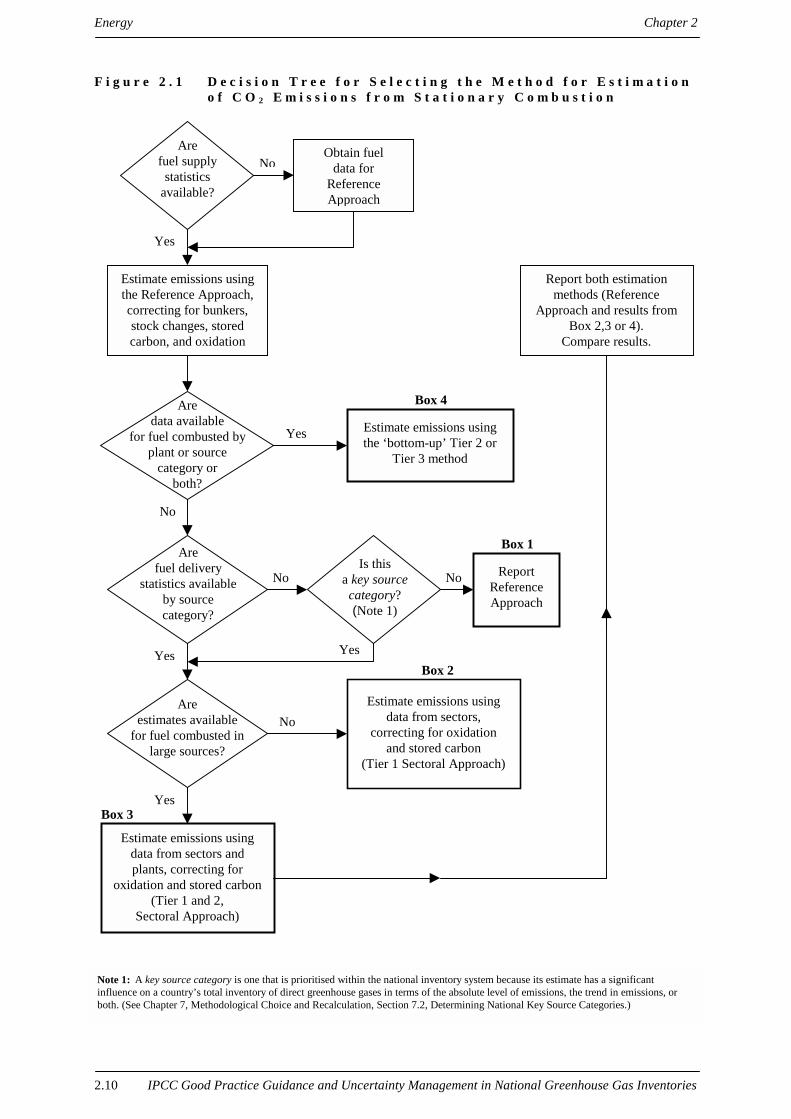
The choice of method is country-specific and is determined by the level of detail of the activity data available asillustrated in Figure 2.1, Decision Tree for Selecting the Method for Estimation of CO2 Emissions fromStationary Combustion. The ‘bottom-up’ approach is generally the most accurate for those countries whoseenergy consumption data are reasonably complete.1 Consequently, inventory agencies should make every effortto use this method if data are available.
Although continuous monitoring is generally recommended because of its high accuracy, it cannot be justified forCO2 alone because of its comparatively high costs and because it does not improve accuracy for CO2. It could,however, be undertaken when monitors are installed for measurements of other pollutants such as SO2 or NOx
where CO2 is monitored as the diluent gas in the monitoring system.2
The Reference Approach provides only aggregate estimates of emissions by fuel type distinguishing betweenprimary and secondary fuels, whereas the Sectoral Approach allocates these emissions by source category. The 1 If the gap between apparent consumption and reported consumption is small, then energy consumption data are probablyreasonably complete.
2 If continuous emissions monitoring were used for certain industrial sources it would be difficult to differentiate emissionsrelated to fuel combustion from emissions related to processing (e.g. cement kilns).

Chapter 2 Energy
IPCC Good Practice Guidance and Uncertainty Management in National Greenhouse Gas Inventories 2.9
aggregate nature of the Reference Approach estimates means that stationary combustion emissions cannot bedistinguished from mobile combustion emissions. Likewise, the Sectoral Approach is not always able todifferentiate between different emission source categories within an economic activity (e.g. between use of gasor oil for heating or for off-road and other mobile machinery in the construction industry).
Estimates of emissions based on the Reference Approach will not be exactly the same as estimates based on theSectoral Approach. The two approaches measure emissions at differing points and use slightly differentdefinitions. However, the differences between the two approaches should not be significant.
For some countries, however, there may be large and systematic differences between estimates developed usingthe two approaches. This will normally indicate a systematic under or overcounting of energy consumption byone method or the other. If this occurs, it is good practice to consult with national statistical authorities and seektheir advice on which method is the most complete and accurate indication of total consumption for each fuel,and use it.
Energy Chapter 2
2.10 IPCC Good Practice Guidance and Uncertainty Management in National Greenhouse Gas Inventories
F i g u r e 2 . 1 D e c i s i o n T r e e f o r S e l e c t i n g t h e M e t h o d f o r E s t i m a t i o no f C O 2 E m i s s i o n s f r o m S t a t i o n a r y C o m b u s t i o n
Arefuel supply
statisticsavailable?
Obtain fueldata for
ReferenceApproach
Estimate emissions usingthe Reference Approach,correcting for bunkers,stock changes, storedcarbon, and oxidation
Aredata available
for fuel combusted byplant or source
category orboth?
Estimate emissions usingthe ‘bottom-up’ Tier 2 or
Tier 3 method
Arefuel delivery
statistics availableby sourcecategory?
Areestimates available
for fuel combusted inlarge sources?
Estimate emissions usingdata from sectors andplants, correcting for
oxidation and stored carbon(Tier 1 and 2,
Sectoral Approach)
Is thisa key sourcecategory?(Note 1)
ReportReferenceApproach
Estimate emissions usingdata from sectors,
correcting for oxidationand stored carbon
(Tier 1 Sectoral Approach)
Report both estimationmethods (Reference
Approach and results fromBox 2,3 or 4).
Compare results.
No
Yes
Box 1
No
YesBox 2
No
YesBox 3
No
Yes
Yes
Box 4
No
Note 1: A key source category is one that is prioritised within the national inventory system because its estimate has a significantinfluence on a country’s total inventory of direct greenhouse gases in terms of the absolute level of emissions, the trend in emissions, orboth. (See Chapter 7, Methodological Choice and Recalculation, Section 7.2, Determining National Key Source Categories.)

Chapter 2 Energy
IPCC Good Practice Guidance and Uncertainty Management in National Greenhouse Gas Inventories 2.11
2.1.1.2 CHOICE OF EMISSION FACTORS AND CALORIFIC VALUES
CO2 emission factors (EF) for fossil fuel combustion depend upon the carbon content of the fuel. The carboncontent of a fuel is an inherent chemical property (i.e. fraction or mass of carbon atoms relative to total number ofatoms or mass) and does not depend upon the combustion process or conditions. The energy content (i.e.calorific value or heating value) of fuels is also an inherent chemical property. However, calorific values varymore widely between and within fuel types, as they are dependent upon the composition of chemical bonds in thefuel. Net calorific values (NCVs) measure the quantity of heat liberated by the complete combustion of a unitvolume or mass of a fuel, assuming that the water resulting from combustion remains as a vapour, and the heat ofthe vapour is not recovered. Gross calorific values, in contrast, are estimated assuming that this water vapour iscompletely condensed and the heat is recovered. Default data in the IPCC Guidelines are based on NCVs.
Emission factors for CO2 from fossil fuel combustion are expressed on a per unit energy basis because the carboncontent of fuels is generally less variable when expressed on a per unit energy basis than when expressed on a perunit mass basis. Therefore, NCVs are used to convert fuel consumption data on a per unit mass or volume basisto data on a per unit energy basis.
Carbon content values can be thought of as potential emissions, or the maximum amount of carbon that couldpotentially be released to the atmosphere if all carbon in the fuels were converted to CO2. As combustionprocesses are not 100% efficient, though, some of the carbon contained in fuels is not emitted to the atmosphere.Rather, it remains behind as soot, particulate matter and ash. Therefore, an oxidation factor is used to account forthe fraction of the potential carbon emissions remaining after combustion.
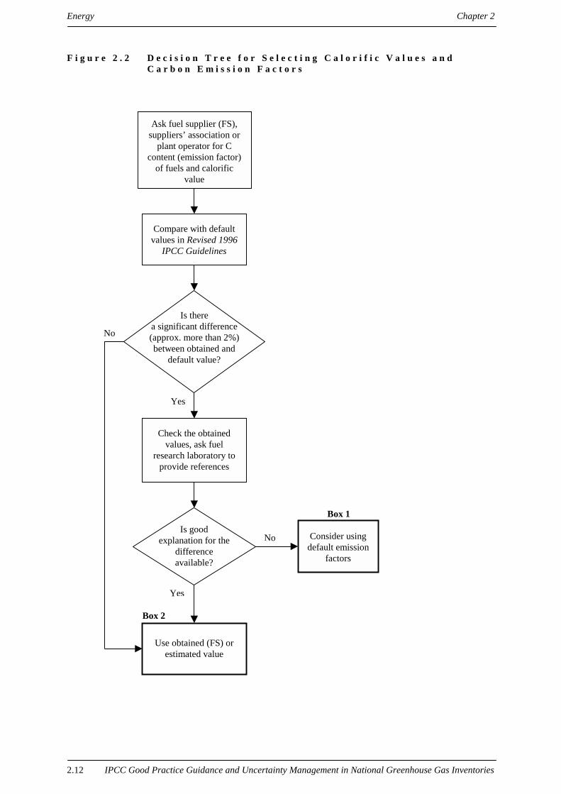
For traded fuels in common circulation, it is good practice to obtain the carbon content of the fuel and netcalorific values from fuel suppliers, and use local values wherever possible. If these data are not available,default values can be used. Figure 2.2, Decision Tree for Selecting Calorific Values and Carbon EmissionFactors illustrates the choice of emission factors.
It may be more difficult to obtain the carbon content and NCV for non-traded fuels, such as municipal solidwaste (MSW) and for fuels that are not sold by heat content, such as crude oil. If necessary, default values areavailable. Values for MSW may be obtained by contacting operators of waste combustion plants for heat raising.The suggested default values for the NCV of municipal solid waste range from 9.5 to 10.5 GJ/t (based oninformation from Sweden and Denmark). The default carbon content of waste is given in Chapter 6, Waste of theIPCC Guidelines. For crude oil, information is available relating the carbon content to the density and the sulfurcontent of the crude oil (see Table 2.2, Typical API Gravities and Sulfur Contents for Various Crude Oil Streamsand Table 2.3, Average API Gravity and Sulfur Content of Imported Crude Oil for Selected Countries Listed inAnnex II of the UN Framework Convention on Climate Change). Information on NCVs for coal types in non-OECD countries is listed in Table 2.4, 1990 country-specific net calorific values. Default net calorific values formost other fuels are available in the Reference Manual of the IPCC Guidelines (Table 1-3, Net Calorific Valuesfor Other Fuels).
Generally, default oxidation factors for gases and oils are known accurately. For coal, oxidation factors aredependent on the combustion conditions and can vary by several percent. It is good practice to discuss the factorswith local users of coal and coal products. However, default factors are also provided in the IPCC Guidelines.
Energy Chapter 2
2.12 IPCC Good Practice Guidance and Uncertainty Management in National Greenhouse Gas Inventories
F i g u r e 2 . 2 D e c i s i o n T r e e f o r S e l e c t i n g C a l o r i f i c V a l u e s a n dC a r b o n E m i s s i o n F a c t o r s
Ask fuel supplier (FS),suppliers’ association or
plant operator for Ccontent (emission factor)
of fuels and calorificvalue
Compare with defaultvalues in Revised 1996
IPCC Guidelines
Is therea significant difference(approx. more than 2%)between obtained and
default value?
Check the obtainedvalues, ask fuel
research laboratory toprovide references
Is goodexplanation for the
differenceavailable?
Use obtained (FS) orestimated value
Consider usingdefault emission
factors
No
Box 1
No
Yes
Box 2
Yes

Chapter 2 Energy
IPCC Good Practice Guidance and Uncertainty Management in National Greenhouse Gas Inventories 2.13
2.1.1.3 CHOICE OF ACTIVITY DATA
Activity data for all tiers are the amount and type of fuel combusted. These data will often be available fromnational energy statistics agencies which collect them directly from the enterprises that consume the fuels or fromindividuals responsible for the combustion equipment. These data are also available from suppliers of fuels whorecord the quantities delivered and the identity of their customers usually as an economic activity code, or from acombination of these sources. Direct collection of fuel consumption data may occur through periodic surveys of asample of enterprises, or, in the case of large combustion plants, through enterprise reports made to the nationalenergy statistics agency or under emission control regulations. Fuel deliveries are well identified for gas, wheremetering is in place, and also for solid and liquid fuels, both of which are distributed to the household and thesmall commercial consumers market.
It is good practice to use fuel combustion statistics rather than delivery statistics where they are available.3Agencies collecting emission data from companies under an environmental reporting regulation could requestfuel combustion data in this context. Fuel combustion data, however, are very seldom complete, since it is notpracticable to measure the fuel consumption or emissions of every residential or commercial source. Hence,national inventories using this approach will generally contain a mixture of combustion data for larger sourcesand delivery data for other sources. The inventory agency must take care to avoid both double counting andomission of emissions when combining data from multiple sources.
Where confidentiality is an issue, direct discussion with the company affected often allows the data to be used. Incases where such permission is not given, aggregation of the fuel consumption or emissions with those from othercompanies is usually sufficient to conceal the identity of the company without understating emissions.
It is necessary to estimate the amount of carbon stored in products for the Reference Approach, and if no detailedcalculation in the Industrial Processes sector is performed. It is good practice to obtain stored carbon factors bycontacting the petrochemical industry that uses the feedstock. A list of fuels/products that accounts for themajority of carbon stored is given in the IPCC Guidelines together with default stored carbon factors. It shouldbe used unless more detailed country-specific information is available. Where data are available for other fuels/products, the estimation of stored carbon is strongly encouraged.4 The default factor for stored carbon inlubricants may be overestimated because waste lubricants are often burned for energy. It is good practice tocontact those responsible for recovering used oils in order to discover the extent to which used oils are burned inthe country.
When using the Reference Approach, fuel supply statistics5 should be used and there may be a choice of sourcefor import and export data. Official customs figures or industry figures may be used. The compilers of nationalenergy data will have made this choice based on their assessment of data quality when preparing national fuelbalances. The choice may differ from fuel to fuel. Thus, it is good practice to consult with the national energystatistics agency when choosing between energy supply and delivery statistics in order to establish whether thecriteria the agency has used in selecting the basis for import and export statistics of each fuel are appropriate forinventory use.
When activity data are not quantities of fuel combusted but instead deliveries to enterprises or main sub-categories, there is a risk of double counting emissions from the Industrial Processes, Solvents or Waste Sectors.Identifying double counting is not always easy. Fuels delivered and used in certain processes may give rise to by-products used as fuels elsewhere in the plant or sold for fuel use to third parties (e.g. blast furnace gas, derivedfrom coke and other carbon inputs to blast furnaces). It is good practice to coordinate estimates between thestationary CO2 source category and relevant industrial categories to avoid double counting or omissions.Appendix 2.1A.1 lists the categories and subcategories where fossil fuel carbon is reported, and between whichdouble counting of fossil fuel carbon could, in principle, occur.
3 Quantities of solid and liquid fuels delivered to enterprises will, in general, differ from quantities combusted by theamounts put into or taken from stocks held by the enterprise. Stock figures shown in national fuel balances may not includestocks held by final consumers, or may include only stocks held by a particular source category (for example electricityproducers). Delivery figures may also include quantities used for mobile sources or as feedstock.
4 The Frauenhofer Institute in Germany is currently undertaking an examination of carbon flows through petrochemicalindustries in a number of countries. It is hoped that this work will result in better estimates of the fraction of petrochemicalfeedstock stored within the products manufactured. The study will be completed by mid-2000.
5 These are national production of primary fuels, and imports, exports and stock changes of all fuels. Oils used forinternational bunkers are treated like exports and excluded from supply.

Energy Chapter 2
2.14 IPCC Good Practice Guidance and Uncertainty Management in National Greenhouse Gas Inventories
For some source categories (e.g. combustion in the Agriculture Sector), there may be some difficulty inseparating fuel used in stationary equipment from fuel used in mobile machinery. Given the different emissionfactors for non-CO2 gases of these two sources, good practice is to derive energy use of each of these sources byusing indirect data (e.g. number of pumps, average consumption, needs for water pumping). Expert judgementand information available from other countries may also be relevant.
2.1.1.4 COMPLETENESS
A complete estimate of emissions from fuel combustion must include emissions from all fuels and all sourcecategories identified within the IPCC Guidelines. A reliable and accurate bottom-up CO2 emissions estimate isimportant because it increases confidence in the underlying activity data. These, in turn, are importantunderpinnings for the calculation of CH4 and N2O emissions from stationary sources.
All fuels delivered by fuel producers must be accounted for, so that sampling errors do not arise. Mis-classification of enterprises and the use of distributors to supply small commercial customers and householdsincrease the chance of systematic errors in the allocation of fuel delivery statistics. Where sample survey data thatprovide figures for fuel consumption by specific economic sectors exist, the figures may be compared with thecorresponding delivery data. Any systematic difference should be identified and the adjustment to the allocationof delivery data may then be made accordingly.
Systematic under-reporting of solid and liquid fuels may also occur if final consumers import fuels directly.Direct imports will be included in customs data and therefore in fuel supply statistics, but not in the statistics offuel deliveries provided by national suppliers. If direct importing by consumers is significant, then the statisticaldifference between supplies and deliveries will reveal the magnitude. Once again, a comparison withconsumption survey results will reveal which main source categories are involved with direct importing.
Experience has shown that the following activities may be poorly covered in existing inventories and theirpresence should be specifically checked:
• Change in producer stocks of fossil fuels;
• Combustion of waste for energy purposes. Waste incineration should be reported in the Waste sourcecategory, combustion of waste for energy purposes should be reported in the Energy source category;
• Energy industries’ own fuel combustion;
• Conversion of petrochemical feedstocks into petrochemical products (carbon storage);
• Fuel combustion for international aviation and marine transport (needed for the Reference Approach).Sections 2.4.1.3 and 2.5.1.3 of this chapter provide more guidance on this subject.
The reporting of emissions from coke use in blast furnaces requires attention. Crude (or pig) iron is typicallyproduced by the reduction of iron oxides ores in a blast furnace, using the carbon in coke (sometimes otherreducing agents) as both the fuel and reducing agent. Since the primary purpose of coke oxidation is to producepig iron, the emissions should be considered as coming from an industrial process if a detailed calculation ofindustrial emissions is being undertaken. It is important not to double-count the carbon from the consumption ofcoke or other fuels. So, if these emissions have been included in the Industrial Processes sector, they should notbe included in the Energy sector. However, there are countries where industrial emissions are not addressed indetail. In these instances, the emissions should be included in the Energy sector. In any case, the amount ofcarbon that is stored in the final product should be subtracted from the effective emissions.
2.1.1.5 DEVELOPING A CONSISTENT TIME SERIES
It is good practice to prepare inventories using the method selected in Figure 2.1, Decision Tree for Selecting theMethod for Estimation of CO2 Emissions from Stationary Combustion for all years in the time series. Where thisis difficult due to a change of methods or data over time, estimates for missing data in the time series should beprepared based on backward extrapolation of present data. When changing from a Reference Approach to ahigher tier approach, inventory agencies should establish a clear relationship between the approaches and applythis to previous years if data are lacking. Chapter 7, Methodological Choice and Recalculation, Section 7.3.2.2,Alternative Recalculation Techniques, provides guidance on various approaches that can be used in this case.

Chapter 2 Energy
IPCC Good Practice Guidance and Uncertainty Management in National Greenhouse Gas Inventories 2.15
2.1.1.6 UNCERTAINTY ASSESSMENT
ACTIVITY DATAThe information in this section can be used in conjunction with the methods outlined in Chapter 6, QuantifyingUncertainties in Practice, to assess overall uncertainties in the national inventory. Chapter 6 explains how to useempirical data and expert judgement to obtain country-specific uncertainty.
The accuracy in determining emission estimates using the Sectoral Approach is almost entirely determined by theavailability of the delivery or combustion statistics for the main source categories. The main uncertainty arisesfrom:
• The adequacy of the statistical coverage of all source categories;
• The adequacy of the coverage of all fuels (both traded and non-traded).
Statistics of fuel combusted at large sources obtained from direct measurement or obligatory reporting are likelyto be within 3% of the central estimate.6 For the energy intensive industries, combustion data are likely to bemore accurate. It is good practice to estimate the uncertainties in fuel consumption for the main sub-categories inconsultation with the sample survey designers because the uncertainties depend on the quality of the surveydesign and size of sample used.
In addition to any systematic bias in the activity data as a result of incomplete coverage of consumption of fuels,the activity data will be subject to random errors in the data collection that will vary from year to year. Countrieswith good data collection systems, including data quality control, may be expected to keep the random error intotal recorded energy use to about 2-3% of the annual figure. This range reflects the implicit confidence limits ontotal energy demand seen in models using historical energy data and relating energy demand to economic factors.Percentage errors for individual energy use activities can be much larger.
Overall uncertainty in activity data is a combination of both systematic and random errors. Most developedcountries prepare balances of fuel supply and deliveries and this provides a check on systematic errors. In thesecircumstances, overall systematic errors are likely to be small. Experts believe that uncertainty resulting from thetwo errors is probably in the range of ±5%. For countries with less well-developed energy data systems, thiscould be considerably larger, probably about ±10%. Informal activities may increase the uncertainty up to asmuch as 50% in some sectors for some countries. See Table 2.6, Level of Uncertainty Associated with StationaryCombustion Activity Data, for more detailed uncertainty estimates.
EMISSION FACTORSThe uncertainty associated with EFs and NCVs results from two main elements, viz. the accuracy with which thevalues are measured, and the variability in the source of supply of the fuel and quality of the sampling ofavailable supplies. There are few mechanisms for systematic errors in the measurement of these properties.Consequently, the errors can be considered mainly random. For traded fuels, the uncertainty is likely to be lessthan 5%. For non-traded fuels, the uncertainty will be higher and will result mostly from variability in the fuelcomposition.
Default uncertainty ranges are not available for stored carbon factors or coal oxidation factors. It is evident,however, that consultation with consumers using the fuels as raw materials or for their non-fuel characteristics isessential for accurate estimations of stored carbon. Similarly, large coal users can provide information on thecompleteness of combustion in the types of equipment they are using.
2 . 1 . 2 R e p o r t i n g a n d d o c u me n t a t i o nIt is good practice to document and archive all information required to produce the national emissions inventoryestimates as outlined in Section 8.10.1 of Chapter 8, Quality Assurance and Quality Control.
It is not practical to include all documentation in the national inventory report. However, the inventory shouldinclude summaries of methods used and references to source data such that the reported emissions estimates aretransparent and steps in their calculation may be retraced. 6 The percentages cited in this section represent an informal polling of assembled experts aiming to approximate the 95%confidence interval around the central estimate.

Energy Chapter 2
2.16 IPCC Good Practice Guidance and Uncertainty Management in National Greenhouse Gas Inventories
Some examples of specific documentation and reporting which are relevant to this source category are providedbelow:
• The sources of the energy data used and observations on the completeness of the data set;
• The sources of the calorific values and the date they were last revised;
• The sources of emission factors and oxidation factors, the date of the last revision and any verification of theaccuracy. If a carbon storage correction has been made, documentation should include the sources of thefactor and how the figures for fuel deliveries have been obtained.
2 . 1 . 3 I n v e n t o r y q u a l i t y a s s u r a n c e / q u a l i t y c o n t r o l( Q A / Q C )
It is good practice to conduct quality control checks as outlined in Chapter 8, Quality Assurance and QualityControl, Table 8.1, Tier 1 General Inventory Level QC Procedures, and expert review of the emission estimates.Additional quality control checks as outlined in Tier 2 procedures in Chapter 8 and quality assurance proceduresmay also be applicable, particularly if higher tier methods are used to determine emissions from this sourcecategory. Inventory agencies are encouraged to use higher tier QA/QC for key source categories as identified inChapter 7, Methodological Choice and Recalculation.
In addition to the guidance in Chapter 8, specific procedures of relevance to this source category are outlinedbelow.
Comparison of emission est imates using different approachesThe inventory agency should compare estimates of CO2 emissions from fuel combustion prepared using theSectoral Tier 1 and Tier 2 Approach with the Reference Approach, and account for any significant differences. Inthis comparative analysis, emissions from fuels other than by combustion, that are accounted for in other sectionsof a GHG inventory, should be subtracted from the Reference Approach (See Appendix 2.1A.1).
Activity data check• The inventory agency should construct national energy balances expressed in mass units, and mass balances
of fuel conversion industries. The time series of statistical differences should be checked for systematiceffects (indicated by the differences persistently having the same sign) and these effects eliminated wherepossible. This task should be done by, or in cooperation with, the national agency in charge of energystatistics.
• The inventory agency should also construct national energy balances expressed in energy units and energybalances of fuel conversion industries. The time series of statistical differences should be checked, and thecalorific values cross-checked with IEA values (see Figure 2.2, Decision Tree for Selecting Calorific Valuesand Carbon Emission Factors). This step will only be of value where different calorific values for aparticular fuel (for example, coal) are applied to different headings in the balance (such as production,imports, coke ovens and households). Statistical differences that change in magnitude or sign significantlyfrom the corresponding mass values provide evidence of incorrect calorific values.
• The inventory agency should confirm that gross carbon supply in the Reference Approach has been adjustedfor fossil fuel carbon from imported or exported non-fuel materials in countries where this is expected to besignificant.
• Energy statistics should be compared with those provided to international organisations to identifyinconsistencies.
• There may be routine collections of emissions and fuel combustion statistics at large combustion plants forpollution legislation purposes. If possible, the inventory agency can use these plant-level data to cross-checknational energy statistics for representativeness.
Emission factors check• The inventory agency should construct national energy balances expressed in carbon units and carbon
balances of fuel conversion industries. The time series of statistical differences should be checked. Statisticaldifferences that change in magnitude or sign significantly from the corresponding mass values provideevidence of incorrect carbon content.

Chapter 2 Energy
IPCC Good Practice Guidance and Uncertainty Management in National Greenhouse Gas Inventories 2.17
• Monitoring systems at large combustion plants may be used to check the emission and oxidation factors inuse at the plant.
Evaluation of direct measurements• The inventory agency should evaluate the quality control associated with facility-level fuel measurements
that have been used to calculate site-specific emission and oxidation factors. If it is established that there isinsufficient quality control associated with the measurements and analysis used to derive the factor,continued use of the factor may be questioned.

Energy Chapter 2
2.18 IPCC Good Practice Guidance and Uncertainty Management in National Greenhouse Gas Inventories
A p p e n d i x 2 . 1 A . 1 R e p o r t i n g o f e mi s s i o n s o f f o s s i lc a r b o n - b a s e d mo l e c u l e s a c c o r d i n g t o t h e R e v i s e d1 9 9 6 I P C C G u i d e l i n e s s o u r c e c a t e g o r i e s
The following table shows where fossil carbon is accounted for and may be used to help identify and eliminatedouble counting as discussed in Section 2.1.1.3. It may also help explain any difference between the ReferenceApproach and Sectoral Approach calculations.
TABLE 2.1
REPORTING OF EMISSIONS OF FOSSIL CARBON-CONTAINING MOLECULES ACCORDING TO THE REVISED 1996 IPCCGUIDELINES SOURCE CATEGORIES7
From fossil fuel carbon From other fossil carbon
1A Fuel combustion
All fossil carbon for combustion purposes
1B Fugitive emissions
Escapes and releases from fossil carbon flows fromextraction point through to final oxidation
2 Industrial Processes 2 Industrial Processes
Ammonia Cement
Silicon carbide Lime production
Calcium carbide Limestone use
Soda ash production, Solvay process(emissions from calcining)
Soda ash production (natural process)
Iron/steel and ferroalloys Soda ash use
Aluminium
Other metals (see IPCC Guidelines Reference Manual,Table 2-21, Production Processes for Some Metals)
Production and use of halocarbons
Organic chemical manufacture
Asphalt manufacture and use
Adipic acid
3 Solvents
6 Waste
Short-life wastes comprising used oils, used solvents andplastics
Long-life wastes comprising plastics entering heat raisingand incineration and degradation in landfills (productsmanufactured before the inventory year)
7 Numbers before source categories correspond to the numbering system of the Revised 1996 IPCC Guidelines, ReportingInstructions, Common Reporting Framework.

Chapter 2 Energy
IPCC Good Practice Guidance and Uncertainty Management in National Greenhouse Gas Inventories 2.19
A p p e n d i x 2 . 1 A . 2 M e t h o d t o e s t i ma t e c a r b o nc o n t e n t b a s e d o n A P I 8 g r a v i t y a n d s u l f u r c o n t e n t
The following formula is based on the analyses of 182 crude oil samples and may be used to estimate the carboncontent of crude oil. (Source: USDOE/EIA. URL: http://www.eia.doe.gov/oiaf/1605/gg98rpt/appendixb.html)
EQUATION 2.1Carbon Content = 76.99 + (10.19 • SG) – (0.76 • Sulfur Content)
Where:
SG denotes the specific gravity of the oil
Carbon and Sulfur content are measured in percent by weight
Specific Gravity may be calculated from the API gravity figure using:
EQUATION 2.2SG = 141.5 / (API + 131.5)
Inferred carbon content is calculated based on the specific gravities and the API values in the first 2 columns ofthe following table using the above formula. Note that inferred values may differ from measured values.
8 API: Arbitrary scale designating an oil's specific gravity, or the ratio of the weights of equal volumes of oil and pure water;it is the standard specific gravity scale of the petroleum industry. As volume is dependent on temperature and pressure, thesemust be specified. In the United States they are generally 60 degrees F (16 degrees C) and one atmosphere (101.3 kPa)pressure. The API gravity scale, whose units are degrees API, does not vary linearly with the specific gravity or its relatedproperties (e.g. viscosity), high specific gravity values give low API gravity values using the relationship
degrees API = (141.5 / specific gravity at 60 degrees F) – 131.5
Water with a specific gravity of 1 has an API gravity of 10 degrees. The API scale has the advantage of allowinghydrometers, which measure specific gravity, to be calibrated linearly. The Baumé scale, originally developed by AntoineBaumé for this purpose, was found to be in error and the API scale replaced it in 1921. The Baumé scale, still used in parts ofEurope, is given by the relationship
degrees Baumé = (140 / specific gravity at 60 degrees F) – 130.
Source: adapted from Encyclopaedia Britannica.

Energy Chapter 2
2.20 IPCC Good Practice Guidance and Uncertainty Management in National Greenhouse Gas Inventories
TABLE 2.2
TYPICAL API GRAVITY AND SULFUR CONTENT FOR VARIOUS CRUDE OIL STREAMS
Crude Category Typical APIGravity
Typical SulfurContent (% wt)
Inferred Carbon Content(% wt)
mean orlowervalue
uppervalue
mean orlowervalue
uppervalue
mean orlower value
upper value
Middle East
Murban 39.8 0.8 84.8
Umm Shaif 37.5 1.4 84.5
Upper Zakum 34 1.8 84.3
Lower Zakum 40 1.1 84.6
Abu Dhabi
Other Abu Dhabi 46.7 0.8 84.5
Dubai Dubai 31 32 1.9 84.4 84.4
Sharjah 62.5 0.1 84.3
Iranian Light 34 1.4 84.6
Iranian Heavy 31 1.6 84.6
Iran
Other Iran 32.6 2.1 84.2
Basrah Light 34 2.1 84.1
Kirkuk 36 2 84.1
Iraq
Other Iraq 36.1 2 84.1
Kuwait Kuwait Blend 30 31 2.5 84.0 84.0
Offshore (Khafji/Hout) 28 33 1.9 2.9 83.6 84.6Neutral Zone
Onshore 23 25 3.3 3.9 83.2 83.8
Oman Oman 34 0.8 85.1
Qatar Marine 36 1.5 84.5Qatar
Qatar Land 41 1.2 84.4
Arab Light 33 34 1.7 84.4 84.5
Arab Medium 30 31.5 2.3 84.1 84.2
Arab Heavy 27 28 2.8 83.9 84.0
Berri (Extra Light) 37 38 1.1 1.2 84.6 84.7
Saudi Arabia
Other Saudi Arabia 52.3 0.7 84.3
Syria Light 36 0.6 85.1Syria
Souedie 24 3.9 83.3
Marib Light 40 0.1 85.3
Masila Blend 30 31 0.6 85.4 85.5
Yemen
Other Yemen 41 0.4 85.0

Chapter 2 Energy
IPCC Good Practice Guidance and Uncertainty Management in National Greenhouse Gas Inventories 2.21
TABLE 2.2 (CONTINUED)
TYPICAL API GRAVITY AND SULFUR CONTENT FOR VARIOUS CRUDE OIL STREAMS
Crude Category Typical APIGravity
Typical SulfurContent (% wt)
Inferred Carbon Content(% wt)
mean orlowervalue
uppervalue
mean orlowervalue
uppervalue
mean orlower value
upper value
Other Middle East 31.7 2.1 84.2
Africa
Saharan Blend 44 0.1 85.1Algeria
Other Algeria 45.1 0.1 85.1
Cameroon 32 0.15 85.7
Congo 37.4 0.1 85.5
Medium/Light (30-40o) 31.1 1.9 84.4Egypt
Heavy (<30o API) 27.9 2.1 84.4
Rabi/Rabi Kounga 34 0.1 85.6Gabon
Other Gabon 32.1 0.6 85.3
Light (>40o API) 41.7 0.2 85.2
Medium (30-40o API) 37.2 0.3 85.3
Libya
Heavy (<30o API) 26.2 1.7 84.8
Medium (<33o API) 29.6 0.2 85.8
Light (33-45o API) 36.3 0.2 85.4
Nigeria
Condensate (>45o API) 46.1 0.1 85.0
Tunisia 36.1 0.6 85.1
Zaire 31 0.2 85.7
Other Africa 29.7 0.2 85.8
Asia
Seria Light 36 0.1 85.5Brunei
Champion 25 0.1 86.1
Daqing (Taching) 33 0.1 85.7
Shengli 24 1 85.5
China
Other China 32 0.2 85.7
Minas 34 0.1 85.6
Cinta 33 0.1 85.7
Handil 33 0.1 85.7
Duri 20 0.2 86.4
Arun Condensate 54 0.02 84.7
Indonesia
Other Indonesia 38 0.1 85.4
Tapis 44 0.1 85.1
Labuan 33 0.1 85.7
Malaysia
Other Malaysia 38.9 0.1 85.4
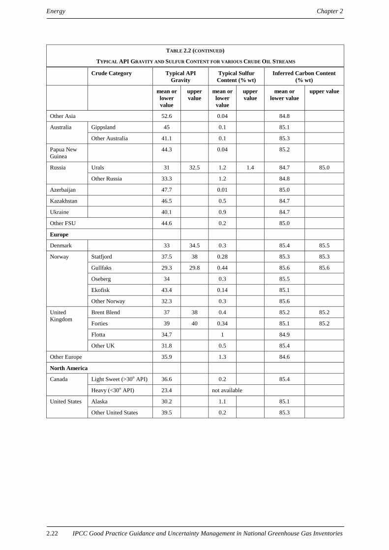
Energy Chapter 2
2.22 IPCC Good Practice Guidance and Uncertainty Management in National Greenhouse Gas Inventories
TABLE 2.2 (CONTINUED)
TYPICAL API GRAVITY AND SULFUR CONTENT FOR VARIOUS CRUDE OIL STREAMS
Crude Category Typical APIGravity
Typical SulfurContent (% wt)
Inferred Carbon Content(% wt)
mean orlowervalue
uppervalue
mean orlowervalue
uppervalue
mean orlower value
upper value
Other Asia 52.6 0.04 84.8
Gippsland 45 0.1 85.1Australia
Other Australia 41.1 0.1 85.3
Papua NewGuinea
44.3 0.04 85.2
Urals 31 32.5 1.2 1.4 84.7 85.0Russia
Other Russia 33.3 1.2 84.8
Azerbaijan 47.7 0.01 85.0
Kazakhstan 46.5 0.5 84.7
Ukraine 40.1 0.9 84.7
Other FSU 44.6 0.2 85.0
Europe
Denmark 33 34.5 0.3 85.4 85.5
Statfjord 37.5 38 0.28 85.3 85.3
Gullfaks 29.3 29.8 0.44 85.6 85.6
Oseberg 34 0.3 85.5
Ekofisk 43.4 0.14 85.1
Norway
Other Norway 32.3 0.3 85.6
Brent Blend 37 38 0.4 85.2 85.2
Forties 39 40 0.34 85.1 85.2
Flotta 34.7 1 84.9
UnitedKingdom
Other UK 31.8 0.5 85.4
Other Europe 35.9 1.3 84.6
North America
Light Sweet (>30o API) 36.6 0.2 85.4Canada
Heavy (<30o API) 23.4 not available
Alaska 30.2 1.1 85.1United States
Other United States 39.5 0.2 85.3

Chapter 2 Energy
IPCC Good Practice Guidance and Uncertainty Management in National Greenhouse Gas Inventories 2.23
TABLE 2.2 (CONTINUED)
TYPICAL API GRAVITY AND SULFUR CONTENT FOR VARIOUS CRUDE OIL STREAMS
Crude Category Typical APIGravity
Typical SulfurContent (% wt)
Inferred Carbon Content(% wt)
mean orlowervalue
uppervalue
mean orlowervalue
uppervalue
mean orlower value
upper value
Latin America
Brazil 20.7 0.5 86.1
Cano Limon 30 0.5 85.5Colombia
Other Colombia 35.8 not available
Oriente 28 29 0.9 1.0 85.2 85.3Ecuador
Other Ecuador not available not available
Maya 22.2 3.3 83.9
Isthmus 34.8 1.5 84.5
Mexico
Olmeca 39.8 0.8 84.8
Peru 20.2 1.3 85.5
Light (>30o API) 32.6 1.1 84.9
Medium (22-30o API) 27.7 1.6 84.8
Heavy (17-22o API) 19.5 2.5 84.6
Venezuela
Extra Heavy (<17o
API)14.5 2.8 84.7
Source for API gravity and sulfur content: International Energy Agency.

Energy Chapter 2
2.24 IPCC Good Practice Guidance and Uncertainty Management in National Greenhouse Gas Inventories
TABLE 2.3
AVERAGE API GRAVITY AND SULFUR CONTENT OF IMPORTED CRUDE OIL FOR SELECTED COUNTRIES LISTED INANNEX II OF THE UN FRAMEWORK CONVENTION ON CLIMATE CHANGE
Average API Gravity Average Sulfur(% weight)
Inferred Carbon Content(% weight)
Australia 39.9 0.34 85.1
Austria 37.4 0.84 84.9
Belgium 32.8 1.25 84.8
Canada 32.4 0.90 85.1
Denmark 40.9 0.22 85.2
Finland 35.8 0.54 85.2
France 35.8 1.01 84.8
Germany 36.5 0.76 85.0
Greece 33.9 1.65 84.5
Ireland 36.9 0.25 85.4
Italy 34.1 1.15 84.8
Japan 34.8 1.51 84.5
Netherlands 33.3 1.45 84.6
New Zealand 34.4 1.01 84.9
Norway 33.3 0.39 85.4
Portugal 33.2 1.39 84.7
Spain 31.5 1.36 84.8
Sweden 34.5 0.76 85.1
Switzerland 39.4 0.46 85.1
Turkey 34.2 1.48 84.6
UnitedKingdom
35.9 0.64 85.1
United States 30.3 not available
Average API gravity and sulfur content has been calculated from imports into the above countries in 1998. Values will change over timedue to changes in crude streams that are imported. Any domestic crude oil consumed in the country would also need to be taken intoaccount.
Source for API gravity and sulfur content: International Energy Agency.

Chapter 2 Energy
IPCC Good Practice Guidance and Uncertainty Management in National Greenhouse Gas Inventories 2.25
A p p e n d i x 2 . 1 A . 31 9 9 0 a c o u n t r y - s p e c i f i c n e t c a l o r i f i c v a l u e sThe following table is an update from the table supplied in the Revised 1996 IPCC Guidelines. It contains moredisaggregated information on coal. Some values have been revised by the International Energy Agency.
TABLE 2.4
1990a COUNTRY-SPECIFIC NET CALORIFIC VALUESb
(Terajoule perkilotonne)
Albania Algeria AngolaCabinda
Argentina Armenia Australia Austria Azer-baijan
Bahrain Bangla-desh
Belarus
OIL
Crude Oil 41.45 43.29 42.75 42.29 - 43.21 42.75 42.08 42.71 42.16 42.08
NGL - 43.29 - 42.50 - 45.22 45.22 41.91 42.71 42.71 -
Refinery Feedst. - - - - - 42.50 42.50 - - - -
COAL
Coking Coal
Production - 25.75 - - - 28.34 - - - - -
Imports 27.21 25.75 - 30.14 - - 28.00 - - - -
Exports - - - - - 28.21 - - - - -
Other Bituminous Coal and Anthracitec
Production - - - 24.70 - 24.39 - - - - -
Imports 27.21 - - - 18.58 - 28.00 18.58 - 20.93 25.54
Exports - - - 24.70 - 25.65 - - - - 25.54
Sub-Bituminous Coal
Production - - - - - 17.87 - - - - -
Imports - - - - - - - - - - -
Exports - - - - - - - - - - -
Lignite
Production 9.84 - - - - 9.31 10.90 - - - -
Imports - - - - - - 10.90 - - - -
Exports 9.84 - - - - - 10.90 - - - -
Coal Products
Patent Fuel - - - - - - - - - - -
BKB - - - - - 21.00 19.30 - - - 8.37
Coke Oven Coke 27.21 27.21 - 28.46 - 25.65 28.20 - - - 25.12
Gas Coke - - - - - - - - - - -a For the former Soviet and Yugoslav Republics, 1996 numbers have been used.b The NCVs are those used by the IEA in the construction of energy balances.c In IEA statistics, Anthracite is combined with Other Bituminous Coal – the NCVs given above reflect this combination.
Source: Energy Balances of OECD Countries, and Energy Statistics and Balances of Non-OECD Countries.
OECD/IEA, Paris, 1998.

Energy Chapter 2
2.26 IPCC Good Practice Guidance and Uncertainty Management in National Greenhouse Gas Inventories
TABLE 2.4 (CONTINUED)
1990a COUNTRY-SPECIFIC NET CALORIFIC VALUESb
(Terajoule perkilotonne)
Belgium Benin Bolivia Bosnia-Herze-govina
Brazil Brunei Bulgaria Cameroon Canada Chile China
OIL
Crude Oil 42.75 42.58 43.33 - 45.64 42.75 42.62 42.45 42.79 42.91 42.62
NGL - - 43.33 - 45.22 42.75 - - 45.22 42.87 -
Refinery Feedst. 42.50 - - - - 41.87 - - - - -
COAL
Coking Coal
Production - - - - 26.42 - - - 28.78 - 20.52
Imports 29.31 - - - 30.69 - 24.70 - 27.55 28.43 20.52
Exports - - - - - - - - 28.78 - 20.52
Other Bituminous Coal and Anthracite c
Production 25.00 - - - 15.99 - 24.70 - 28.78 28.43 20.52
Imports 25.00 - - - - - 24.70 - 27.55 28.43 20.52
Exports 25.00 - - - - - - - 28.78 - 20.52
Sub-Bituminous Coal
Production 18.10 - - - - - - - 17.38 - -
Imports - - - - - - - - - - -
Exports 18.20 - - - - - - - - - -
Lignite
Production - - - 8.89 - - 7.03 - 14.25 17.17 -
Imports 21.56 - - - - - - - - - -
Exports - - - - - - - - 14.25 - -
Coal Products
Patent Fuel 29.31 - - - - - - - - - -
BKB 20.10 - - - - - 20.10 - - - -
Coke Oven Coke 29.31 - - - 30.56 - 27.21 - 27.39 28.43 28.47
Gas Coke - - - - - - - - - - -a For the former Soviet and Yugoslav Republics, 1996 numbers have been used.b The NCVs are those used by the IEA in the construction of energy balances.c In IEA statistics, Anthracite is combined with Other Bituminous Coal – the NCVs given above reflect this combination.
Source: Energy Balances of OECD Countries, and Energy Statistics and Balances of Non-OECD Countries.
OECD/IEA, Paris, 1998.

Chapter 2 Energy
IPCC Good Practice Guidance and Uncertainty Management in National Greenhouse Gas Inventories 2.27
TABLE 2.4 (CONTINUED)
1990a COUNTRY-SPECIFIC NET CALORIFIC VALUESb
(Terajoule perkilotonne)
Colombia Congo Costa Rica Croatia Cuba Cyprus CzechRepublic
DemocraticRepublic ofCongo
Denmark DominicanRepublic
OIL
Crude Oil 42.24 42.91 42.16 42.75 41.16 42.48 41.78 42.16 42.71 42.16
NGL 41.87 - - 45.22 - - - - - -
Refinery Feedst. - - - - - - - - 42.50 -
COAL
Coking Coal
Production 27.21 - - - - - 24.40 - - -
Imports - - - - - - - - - -
Exports 27.21 - - - - - 27.46 - - -
Other Bituminous Coal and Anthracitec
Production 27.21 - - 25.12 - - 18.19 25.23 - -
Imports - - 25.75 29.31 25.75 25.75 18.19 25.23 26.09 25.75
Exports 27.21 - - - - - 18.19 - 26.09 -
Sub-Bituminous Coal
Production - - - - - - 12.29 - - -
Imports - - - - - - - - - -
Exports - - - - - - 21.28 - - -
Lignite
Production - - - - - - 12.29 - - -
Imports - - - 14.60 - - - - - -
Exports - - - - - - - - - -
Coal Products
Patent Fuel - - - - - - - 29.31 - -
BKB - - - - - - 21.28 - 18.27 -
Coke Oven Coke 20.10 - 27.21 29.31 27.21 - 27.01 27.21 31.84 -
Gas Coke - - - - - - - - - -a For the former Soviet and Yugoslav Republics, 1996 numbers have been used.b The NCVs are those used by the IEA in the construction of energy balances.c In IEA statistics, Anthracite is combined with Other Bituminous Coal – the NCVs given above reflect this combination.
Source: Energy Balances of OECD Countries, and Energy Statistics and Balances of Non-OECD Countries.
OECD/IEA, Paris, 1998.
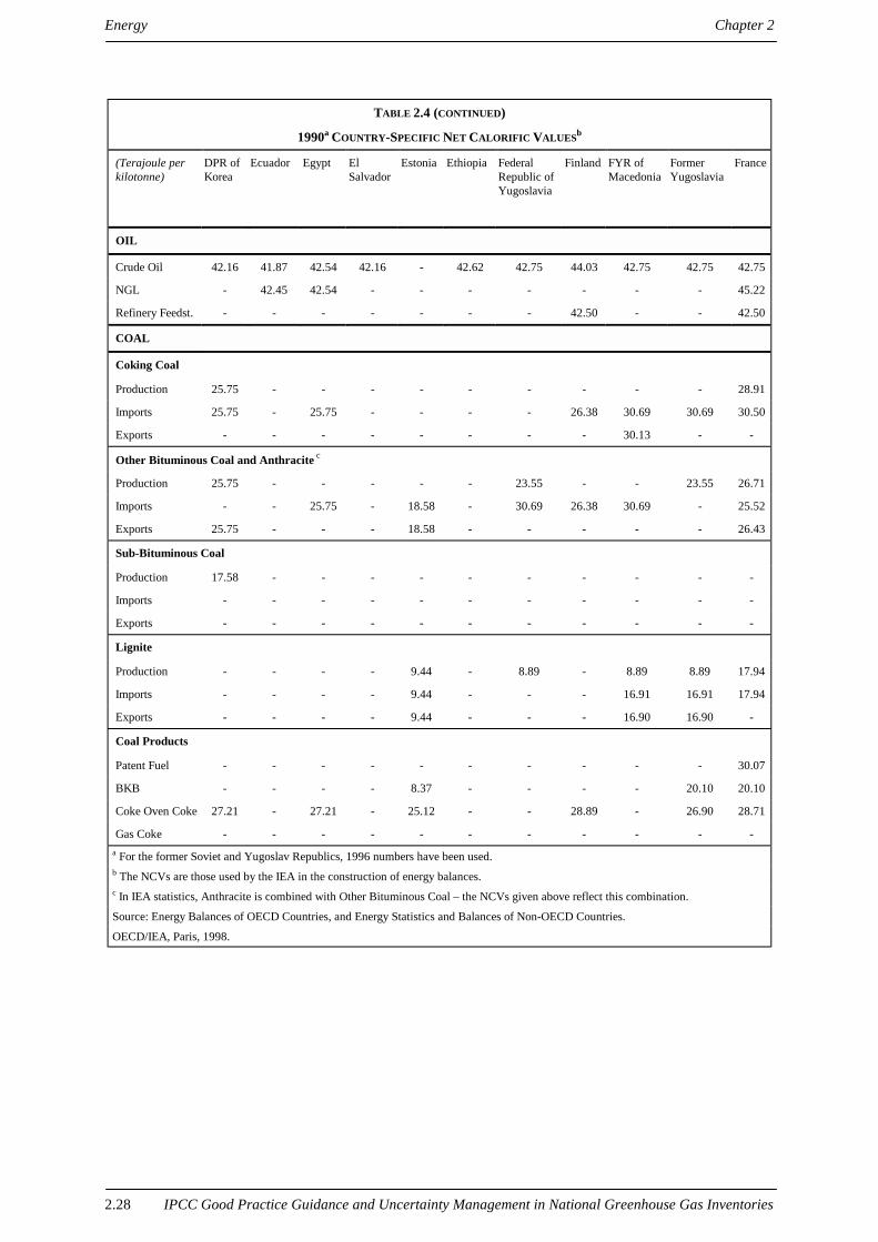
Energy Chapter 2
2.28 IPCC Good Practice Guidance and Uncertainty Management in National Greenhouse Gas Inventories
TABLE 2.4 (CONTINUED)
1990a COUNTRY-SPECIFIC NET CALORIFIC VALUESb
(Terajoule perkilotonne)
DPR ofKorea
Ecuador Egypt ElSalvador
Estonia Ethiopia FederalRepublic ofYugoslavia
Finland FYR ofMacedonia
FormerYugoslavia
France
OIL
Crude Oil 42.16 41.87 42.54 42.16 - 42.62 42.75 44.03 42.75 42.75 42.75
NGL - 42.45 42.54 - - - - - - - 45.22
Refinery Feedst. - - - - - - - 42.50 - - 42.50
COAL
Coking Coal
Production 25.75 - - - - - - - - - 28.91
Imports 25.75 - 25.75 - - - - 26.38 30.69 30.69 30.50
Exports - - - - - - - - 30.13 - -
Other Bituminous Coal and Anthracite c
Production 25.75 - - - - - 23.55 - - 23.55 26.71
Imports - - 25.75 - 18.58 - 30.69 26.38 30.69 - 25.52
Exports 25.75 - - - 18.58 - - - - - 26.43
Sub-Bituminous Coal
Production 17.58 - - - - - - - - - -
Imports - - - - - - - - - - -
Exports - - - - - - - - - - -
Lignite
Production - - - - 9.44 - 8.89 - 8.89 8.89 17.94
Imports - - - - 9.44 - - - 16.91 16.91 17.94
Exports - - - - 9.44 - - - 16.90 16.90 -
Coal Products
Patent Fuel - - - - - - - - - - 30.07
BKB - - - - 8.37 - - - - 20.10 20.10
Coke Oven Coke 27.21 - 27.21 - 25.12 - - 28.89 - 26.90 28.71
Gas Coke - - - - - - - - - - -a For the former Soviet and Yugoslav Republics, 1996 numbers have been used.b The NCVs are those used by the IEA in the construction of energy balances.c In IEA statistics, Anthracite is combined with Other Bituminous Coal – the NCVs given above reflect this combination.
Source: Energy Balances of OECD Countries, and Energy Statistics and Balances of Non-OECD Countries.
OECD/IEA, Paris, 1998.

Chapter 2 Energy
IPCC Good Practice Guidance and Uncertainty Management in National Greenhouse Gas Inventories 2.29
TABLE 2.4 (CONTINUED)
1990a COUNTRY-SPECIFIC NET CALORIFIC VALUESb
(Terajoule perkilotonne)
Gabon Georgia Germany Ghana Greece Guatemala Haiti Honduras HongKong,China
Hungary Iceland
OIL
Crude Oil 42.62 42.08 42.75 42.62 42.75 42.45 - 42.16 - 41.00 -
NGL - - - - 45.22 - - - - 45.18 -
Refinery Feedst. - - 42.50 - 42.50 - - - - 42.08 -
COAL
Coking Coal
Production - - 28.96 - - - - - - 29.61 -
Imports - - 28.96 - - - - - - 30.76 29.01
Exports - - 28.96 - - - - - - - -
Other Bituminous Coal and Anthracite c
Production - 18.58 24.96 - - - - - - 13.15 -
Imports - 18.58 26.52 25.75 27.21 - 25.75 - 25.75 21.50 29.01
Exports - 18.58 31.71 - - - - - - 20.15 -
Sub-Bituminous Coal
Production - - - - - - - - - - -
Imports - - - - - - - - - - -
Exports - - - - - - - - - - -
Lignite
Production - - 8.41 - 5.74 - - - - 9.17 -
Imports - - 14.88 - - - - - - 15.46 -
Exports - - 8.40 - - - - - - - -
Coal Products
Patent Fuel - - 31.40 - - - - - - 16.80 -
BKB - - 20.58 - 15.28 - - - - 21.23 -
Coke Oven Coke - - 28.65 - 29.30 - - 27.21 27.21 27.13 26.65
Gas Coke - - - - - - - - - - -a For the former Soviet and Yugoslav Republics, 1996 numbers have been used.b The NCVs are those used by the IEA in the construction of energy balances.c In IEA statistics, Anthracite is combined with Other Bituminous Coal – the NCVs given above reflect this combination.
Source: Energy Balances of OECD Countries, and Energy Statistics and Balances of Non-OECD Countries.
OECD/IEA, Paris, 1998.

Energy Chapter 2
2.30 IPCC Good Practice Guidance and Uncertainty Management in National Greenhouse Gas Inventories
TABLE 2.4 (CONTINUED)
1990a COUNTRY-SPECIFIC NET CALORIFIC VALUESb
(Terajoule perkilotonne)
India Indonesia Iran Iraq Ireland Israel Italy IvoryCoast
Jamaica Japan Jordan
OIL
Crude Oil 42.79 42.66 42.66 42.83 42.83 42.54 42.75 42.62 42.16 42.62 42.58
NGL 43.00 42.77 42.54 42.83 - - 45.22 - - 46.05 -
Refinery Feedst. - - - - 42.50 - 42.50 - - 42.50 -
COAL
Coking Coal
Production 19.98 - 25.75 - - - - - - 30.63 -
Imports 25.75 - 25.75 - 29.10 - 30.97 - - 30.23 -
Exports - - - - - - - - - - -
Other Bituminous Coal and Anthracitec
Production 19.98 25.75 25.75 - 26.13 - 26.16 - - 23.07 -
Imports 25.75 25.75 - - 29.98 26.63 26.16 - 25.75 24.66 -
Exports 19.98 25.75 - - 26.13 - - - - - -
Sub-Bituminous Coal
Production - - - - - - - - - - -
Imports - - - - - - - - - - -
Exports - - - - - - - - - - -
Lignite
Production 9.80 - - - - 4.19 10.47 - - - -
Imports - - - - 19.82 - 10.47 - - - -
Exports - - - - 19.82 - - - - - -
Coal Products
Patent Fuel - - - - - - - - - 27.05 -
BKB 20.10 - - - 20.98 - - - - - -
Coke Oven Coke 27.21 27.21 27.21 - 32.66 - 29.30 - - 28.64 -
Gas Coke - - - - - - - - - 28.64 -a For the former Soviet and Yugoslav Republics, 1996 numbers have been used.b The NCVs are those used by the IEA in the construction of energy balances.c In IEA statistics, Anthracite is combined with Other Bituminous Coal – the NCVs given above reflect this combination.
Source: Energy Balances of OECD Countries, and Energy Statistics and Balances of Non-OECD Countries.
OECD/IEA, Paris, 1998.

Chapter 2 Energy
IPCC Good Practice Guidance and Uncertainty Management in National Greenhouse Gas Inventories 2.31
TABLE 2.4 (CONTINUED)
1990a COUNTRY-SPECIFIC NET CALORIFIC VALUESb
(Terajoule perkilotonne)
Kazakhstan Kenya Korea Kuwait Kyrgyzstan Latvia Lebanon Libya Lithuania Luxem-bourg
Malaysia
OIL
Crude Oil 42.08 42.08 42.71 42.54 42.08 - 42.16 43.00 42.08 - 42.71
NGL 41.91 - - 42.62 - - - 43.00 - - 43.12
Refinery Feedst. - - - - - - - - 44.80 - 42.54
COAL
Coking Coal
Production 18.58 - - - - - - - - - -
Imports 18.58 - 27.21 - - - - - - - -
Exports 18.58 - - - - - - - - - -
Other Bituminous Coal and Anthracitec
Production 18.58 - 19.26 - 18.58 - - - - - 25.75
Imports 18.58 25.75 27.21 - 18.58 18.58 - - 18.59 29.30 25.75
Exports 18.58 - - - 18.58 25.12 - - 18.59 - 25.75
Sub-Bituminous Coal
Production - - - - - - - - - - -
Imports - - - - - - - - - - -
Exports - - - - - - - - - - -
Lignite
Production 14.65 - - - 14.65 - - - - - -
Imports 18.58 - - - 14.65 - - - - 20.03 -
Exports 18.58 - - - - - - - - - -
Coal Products
Patent Fuel - - - - - - - - - - -
BKB - - - - - 8.37 - - 8.37 20.10 -
Coke Oven Coke 25.12 - 27.21 - - 25.12 - - - 28.50 27.21
Gas Coke - - - - - - - - - - -a For the former Soviet and Yugoslav Republics, 1996 numbers have been used.b The NCVs are those used by the IEA in the construction of energy balances.c In IEA statistics, Anthracite is combined with Other Bituminous Coal - the NCVs given above reflect this combination.
Source: Energy Balances of OECD Countries, and Energy Statistics and Balances of Non-OECD Countries.
OECD/IEA, Paris, 1998.

Energy Chapter 2
2.32 IPCC Good Practice Guidance and Uncertainty Management in National Greenhouse Gas Inventories
TABLE 2.4 (CONTINUED)
1990a COUNTRY-SPECIFIC NET CALORIFIC VALUESb
(Terajoule perkilotonne)
Malta Mexico Moldova Morocco Mozam-bique
Myanmar Nepal Nether-lands
Nether-landsAntilles
NewZealand
Nica-ragua
OIL
Crude Oil - 42.35 - 38.94 - 42.24 - 42.71 42.16 45.93 42.16
NGL - 46.81 - - - 42.71 - 45.22 - 49.75 -
Refinery Feedst. - - - - - - - - - 47.22 -
COAL
Coking Coal
Production - 24.72 - - - - - - - 28.00 -
Imports - 30.18 - - - - - 28.70 - 28.00 -
Exports - 22.41 - - - - - - - 28.00 -
Other Bituminous Coal and Anthracitec
Production - - - 23.45 25.75 25.75 - - - 26.00 -
Imports 25.75 - 18.58 27.63 25.75 25.75 25.12 26.60 - - -
Exports - - - - - - - 26.60 - - -
Sub-Bituminous Coal
Production - 18.20 - - - - - - - 21.30 -
Imports - - - - - - - - - - -
Exports - - - - - - - - - - -
Lignite
Production - - - - - 8.37 - - - 14.10 -
Imports - - - - - - - 20.00 - - -
Exports - - - - - - - 20.00 - - -
Coal Products
Patent Fuel - - - - - - - 29.30 - - -
BKB - - - - - - - 20.00 - - -
Coke Oven Coke - 27.96 25.12 27.21 - 27.21 - 28.50 - - -
Gas Coke - - - - - - - - - - -a For the former Soviet and Yugoslav Republics, 1996 numbers have been used.b The NCVs are those used by the IEA in the construction of energy balances.c In IEA statistics, Anthracite is combined with Other Bituminous Coal – the NCVs given above reflect this combination.
Source: Energy Balances of OECD Countries, and Energy Statistics and Balances of Non-OECD Countries.
OECD/IEA, Paris, 1998.

Chapter 2 Energy
IPCC Good Practice Guidance and Uncertainty Management in National Greenhouse Gas Inventories 2.33
TABLE 2.4 (CONTINUED)
1990a COUNTRY-SPECIFIC NET CALORIFIC VALUESb
(Terajoule perkilotonne)
Nigeria Norway Oman Pakistan Panama Paraguay Peru Philip-pines
Poland Portugal Qatar
OIL
Crude Oil 42.75 42.96 42.71 42.87 42.16 42.54 42.75 42.58 41.27 42.71 42.87
NGL 42.75 45.22 42.71 42.87 - - 42.75 - - - 43.00
Refinery Feedst. - 42.50 - - - - - - 44.80 42.50 -
COAL
Coking Coal
Production - - - - - - - - - - -
Imports - - - 27.54 - - 29.31 - - 29.30 -
Exports - - - - - - - - - - -
Other Bituminous Coal and Anthracite c
Production 25.75 28.10 - 18.73 - - 29.31 20.10 22.95 - -
Imports - 28.10 - - 25.75 - - 20.52 29.41 26.59 -
Exports 25.75 28.10 - - - - - - 25.09 - -
Sub-Bituminous Coal
Production - - - - - - - - - 17.16 -
Imports - - - - - - - - - - -
Exports - - - - - - - - - - -
Lignite
Production - - - - - - - 8.37 8.36 - -
Imports - - - - - - - - - - -
Exports - - - - - - - - 9.00 - -
Coal Products
Patent Fuel - - - - - - - - 22.99 - -
BKB - - - - - - - - 17.84 - -
Coke Oven Coke 27.21 28.50 - 27.21 - - 27.21 27.21 27.85 28.05 -
Gas Coke - - - - - - - - - - -a For the former Soviet and Yugoslav Republics, 1996 numbers have been used.b The NCVs are those used by the IEA in the construction of energy balances.c In IEA statistics, Anthracite is combined with Other Bituminous Coal – the NCVs given above reflect this combination.
Source: Energy Balances of OECD Countries, and Energy Statistics and Balances of Non-OECD Countries.
OECD/IEA, Paris, 1998.

Energy Chapter 2
2.34 IPCC Good Practice Guidance and Uncertainty Management in National Greenhouse Gas Inventories
TABLE 2.4 (CONTINUED)
1990a COUNTRY-SPECIFIC NET CALORIFIC VALUESb
(Terajoule perkilotonne)
Romania Russia SaudiArabia
Senegal Singa-pore
SlovakRepublic
Slovenia SouthAfrica
Spain Sri Lanka Sudan
OIL
Crude Oil 40.65 42.08 42.54 42.62 42.71 41.78 42.75 38.27 42.66 42.16 42.62
NGL - - 42.62 - - 45.18 - - 45.22 - -
Refinery Feedst. - - - - - - 42.50 - 42.50 - -
COAL
Coking Coal
Production 16.33 18.58 - - - - - 30.99 29.16 - -
Imports 25.12 25.12 - - - 23.92 30.69 - 30.14 - -
Exports - 18.58 - - - - - 30.99 - - -
Other Bituminous Coal and Anthracitec
Production 16.33 18.58 - - - - - 23.60 21.07 - -
Imports 25.12 18.58 - - - 23.92 30.69 - 25.54 25.75 -
Exports - 18.58 - - - - - 27.99 23.00 - -
Sub-Bituminous Coal
Production - - - - - - 8.89 - 11.35 - -
Imports - - - - - - 16.91 - 11.35 - -
Exports - - - - - - 16.90 - - - -
Lignite
Production 7.24 14.65 - - - 12.26 8.89 - 7.84 - -
Imports 7.24 - - - 9.67 12.20 16.91 - - - -
Exports - 14.65 - - - 15.26 16.90 - - - -
Coal Products
Patent Fuel 14.65 - - - - - - - 29.30 - -
BKB 14.65 20.10 - - - 21.28 - - 20.22 - -
Coke Oven Coke 20.81 25.12 - - 27.21 27.01 26.90 27.88 30.14 - -
Gas Coke - - - - - - - - - - -a For the former Soviet and Yugoslav Republics, 1996 numbers have been used.b The NCVs are those used by the IEA in the construction of energy balances.c In IEA statistics, Anthracite is combined with Other Bituminous Coal – the NCVs given above reflect this combination.
Source: Energy Balances of OECD Countries, and Energy Statistics and Balances of Non-OECD Countries.
OECD/IEA, Paris, 1998.

Chapter 2 Energy
IPCC Good Practice Guidance and Uncertainty Management in National Greenhouse Gas Inventories 2.35
TABLE 2.4 (CONTINUED)
1990a COUNTRY-SPECIFIC NET CALORIFIC VALUESb
(Terajoule perkilotonne)
Sweden Switzerland Syria Tajikistan Tanzania Thailand TrinidadandTobago
Tunisia Turkey Turk-menistan
Ukraine
OIL
Crude Oil 42.75 43.22 42.04 42.08 42.62 42.62 42.24 43.12 42.79 42.08 42.08
NGL - - - 41.91 - 46.85 - 43.12 - 41.91 -
Refinery Feedst. 42.50 43.70 - - - - - - 42.50 - -
COAL
Coking Coal
Production - - - - 25.75 - - - 32.56 - 21.59
Imports 30.00 - - - - - - - 33.54 - -
Exports - - - - - - - - - - 21.59
Other Bituminous Coal and Anthracitec
Production 14.24 - - - 25.75 - - - 30.04 - 21.59
Imports 26.98 28.05 - 18.58 - 26.38 - 25.75 27.89 18.58 25.54
Exports 26.98 28.05 - - - - - - - - 21.59
Sub-Bituminous Coal
Production - - - 14.65 - - - - 18.00 - -
Imports - - - - - - - - - - -
Exports - - - - - - - - - - -
Lignite
Production - - - - - 12.14 - - 9.63 - 14.65
Imports 8.37 - - - - - - - 12.56 - 14.65
Exports - - - - - - - - - - 14.65
Coal Products
Patent Fuel - 28.05 - - - - - - - - 29.31
BKB 20.10 20.10 - - - - - - 20.93 - -
Coke Oven Coke 28.05 28.05 - - 27.21 27.21 - 27.21 29.31 - 25.12
Gas Coke - - - - - - - - 27.21 - -a For the former Soviet and Yugoslav Republics, 1996 numbers have been used.b The NCVs are those used by the IEA in the construction of energy balances.c In IEA statistics, Anthracite is combined with Other Bituminous Coal – the NCVs given above reflect this combination.
Source: Energy Balances of OECD Countries, and Energy Statistics and Balances of Non-OECD Countries.
OECD/IEA, Paris, 1998.

Energy Chapter 2
2.36 IPCC Good Practice Guidance and Uncertainty Management in National Greenhouse Gas Inventories
TABLE 2.4 (CONTINUED)
1990a COUNTRY-SPECIFIC NET CALORIFIC VALUESb
(Terajoule perkilotonne)
UnitedArabEmirates
UnitedKingdom
UnitedStates
Uruguay Uzbe-kistan
Venezuela Vietnam Yemen Zambia Zimbabwe
OIL
Crude Oil 42.62 43.40 43.12 42.71 42.08 42.06 42.61 43.00 42.16 -
NGL 42.62 46.89 47.69 - 41.91 41.99 - - - -
Refinery Feedst. - 42.50 43.36 - 44.80 - - - - -
COAL
Coking Coal
Production - 29.27 29.68 - - - - - 24.71 25.75
Imports - 30.07 - - - - - - - -
Exports - 29.27 29.68 - - - - - - -
Other Bituminous Coal and Anthracitec
Production - 24.11 26.66 - 18.58 25.75 20.91 - 24.71 25.75
Imports - 26.31 27.69 - 18.58 - - - - 25.75
Exports - 27.53 28.09 - - 25.75 20.91 - 24.71 25.75
Sub-Bituminous Coal
Production - - 19.43 - - - - - - -
Imports - - - - - - - - - -
Exports - - - - - - - - - -
Lignite
Production - - 14.19 - 14.65 - - - - -
Imports - - - - 14.65 - - - - -
Exports - - 14.19 - 14.65 - - - - -
Coal Products
Patent Fuel - 26.26 - - 29.31 - - - - -
BKB - - - - - - - - - -
Coke Oven Coke - 26.54 27.47 27.21 - - 27.21 - 27.21 27.21
Gas Coke - - - - - - - - - -a For the former Soviet and Yugoslav Republics, 1996 numbers have been used.b The NCVs are those used by the IEA in the construction of energy balances.c In IEA statistics, Anthracite is combined with Other Bituminous Coal – the NCVs given above reflect this combination.
Source: Energy Balances of OECD Countries, and Energy Statistics and Balances of Non-OECD Countries.
OECD/IEA, Paris, 1998.

Chapter 2 Energy
IPCC Good Practice Guidance and Uncertainty Management in National Greenhouse Gas Inventories 2.37
2 . 2 N ON - C O 2 E M I S S I O N S F R O M S T A T I O N A R YC O M B U S T I O N
2 . 2 . 1 M e t h o d o l o g i c a l i s s u e sFor stationary sources, some non-CO2 emissions such as methane (CH4), carbon monoxide (CO) and non-methane volatile organic compounds (NMVOC) result from the incomplete combustion of fuels. The IPCCGuidelines cover emissions of stationary combustion-related non-CO2 greenhouse gases from five sectors(Energy and Manufacturing Industries, the Commercial/Institutional Sector, the Residential Sector andAgriculture/Forestry/Fishing sources). This section addresses only emissions of the direct greenhouse gases CH4and N2O.
Fuel characteristics (including the calorific value), the type of technology (including the combustion, operatingand maintenance regime, the size and the vintage of the equipment), and emission controls, are major factorsdetermining rates of emissions of CH4 and N2O gases from stationary sources. Moisture content, carbon fraction,and combustion efficiencies are also important factors to consider.
2.2.1.1 CHOICE OF METHOD
The IPCC Guidelines describe the following general approach to estimate emissions from fuel combustion foreach greenhouse gas and sub-source category:
EQUATION 2.3
Emissions = ∑ (Emission Factorabc • Fuel Consumptionabc)
Where:
a = fuel type
b = sector activity
c = technology type
Given the dependence of emissions on unique combustion conditions and other characteristics, good practice isto disaggregate fuel consumption into smaller, more homogeneous categories, if data and specific emissionfactors are available. The IPCC Guidelines generally refer to such disaggregated estimation methods usingcountry-specific emission factors as Tier 2, and more aggregated estimates as Tier 1 calculations. Good practiceis to use the level of disaggregation that reflects the greatest level of detail in the energy statistics available in thecountry.
Figure 2.3, Decision Tree for Non-CO2 Emissions from Stationary Combustion summarises good practice inmethodological choice. It should be applied separately to each of the sub-source categories for each gas forwhich emissions exist in a country, because the availability of activity data and emission factors (and hence theoutcome in terms of methodological choice) may differ significantly between sub-source categories.
Although continuous measurement of emissions is also consistent with good practice, continuous measurementsof CH4 and N2O alone are not justified because of their comparatively high cost and because practical continuousmonitoring systems are not easily available. Sufficiently accurate results may be obtained by using periodicmeasurements for CH4 and N2O. These measurements would help to improve emission factors. If monitors arealready installed to measure other pollutants, they may deliver some useful parameters such as fluxes.

Energy Chapter 2
2.38 IPCC Good Practice Guidance and Uncertainty Management in National Greenhouse Gas Inventories
F i g u r e 2 . 3 D e c i s i o n T r e e f o r N o n - C O 2 E m i s s i o n s f r o m S t a t i o n a r yC o m b u s t i o n
Aredirect emissionsmeasurements
available?
Arefuel consumptiondata available for
technologytypes?
Is thisa key sourcecategory?(Note 1)
Obtain activity dataand disaggregate by
technology type
Collect or estimateenergy statistics on anaggregated fuel andsource sector level
Calculate emissionsusing IPCC default
Tier 1 emission factors
Arecountry-specificemission factors
available?
Areregional emission
factorsavailable?
Calculate emissionsusing IPCC default
Tier 2 emission factors
Calculate emissionsusing Tier 2 national
emission factors
Calculate emissionsusing Tier 2 regional
emission factors
Estimate emissionsusing measured data
No
Box 1
No
Yes
Box 2
No
Yes
Box 3
No
Yes
Box 4
No
Yes
Yes
Box 5
Note 1: A key source category is one that is prioritised within the national inventory system because its estimate has a significantinfluence on a country’s total inventory of direct greenhouse gases in terms of the absolute level of emissions, the trend in emissions, orboth. (See Chapter 7, Methodological Choice and Recalculation, Section 7.2, Determining National Key Source Categories.)
Note 2: The decision tree and key source category determination should be applied to methane and nitrous oxide emissions separately.

Chapter 2 Energy
IPCC Good Practice Guidance and Uncertainty Management in National Greenhouse Gas Inventories 2.39
Proper use of the decision tree requires an inventory agency to undertake, beforehand, a thorough survey ofavailable national activity data and national or regional emission factor data, by relevant source category. Forsome sub-source categories, activity and emissions data may be sparse. In this case, it is good practice toimprove data quality if an initial calculation with a default method indicates a significant contribution to totalnational emissions or the presence of a high level of uncertainty.
Where direct measurements are available, reporting of implied emission factors cross referenced by technologytype would be helpful, since this information could help others to estimate national emissions.
2.2.1.2 CHOICE OF EMISSION FACTORS
Good practice is to use the most disaggregated technology-specific and country-specific emission factorsavailable, particularly those derived from direct measurements at the different stationary combustion sources.Using the Tier 2 approach, there are three possible types of emission factors:
• National emission factors.9 These emission factors may be developed by national programmes alreadymeasuring emissions of indirect greenhouse gases such as NOx, CO and NMVOC for local air quality;
• Regional emission factors;10
• IPCC default emission factors, provided that a careful review of the consistency of these factors with thecountry conditions has been made. IPCC default factors may be used when no other information is available.
If national activity data are not sufficiently disaggregated to enable the use of Tier 2, then aggregate Tier 1emission factors should be applied, provided that no other referenced data are available that are morerepresentative of combustion conditions within the country.
Emission factors for biomass fuels are not as well developed as those for fossil fuels. Preliminary results from aninternational biomass emission factor research project, focusing on developing countries (e.g. India, Kenya, andChina) show emission factors for small biomass devices and carbonisation that are different from the IPCCdefaults. Given the importance of biomass in many countries, it is suggested that country experts consider thenew well-researched emission factors as soon as they are published (Smith et al., 1993; Smith et al., 1999; Smithet al., 2000; Zhang et al., 1999; Zhang et al., 2000).
2.2.1.3 CHOICE OF ACTIVITY DATA
Due to the technology-specific nature of non-CO2 formation, detailed fuel combustion technology statistics areneeded in order to provide rigorous emission estimates. It is good practice to collect activity data in units of fuelused, and to disaggregate as far as possible into the share of fuel used by major technology types. Disaggregationcan be achieved through a bottom-up survey of fuel consumption and combustion technology, or through top-down allocations based on expert judgement and statistical sampling. Specialised statistical offices or ministerialdepartments are generally in charge of regular data collection and handling. Inclusion of representatives fromthese departments in the inventory process could facilitate the acquisition of appropriate activity data.
Good practice for electricity autoproduction (self-generation) is to assign emissions to the source categories (orsub-source categories) where they were generated and to identify them separately from those associated withother end-uses such as process heat. In many countries, the statistics related to autoproduction are available andregularly updated. Therefore, activity data do not represent a serious obstacle to estimating non-CO2 emissions inthose countries.
For some source categories (e.g. energy use in agriculture), there may be some difficulties in separating fuel usedin stationary equipment from fuel used in mobile machinery. Given the different emission factors of these twosources, good practice is to derive the energy use of each of these sources by using indirect data (e.g. number ofpumps, average consumption, and needs for water pumping). Expert judgement and information available fromother countries may also be relevant.
9 Since the associated uncertainty ranges are dependent on the instrumentation used and on the frequency of measurements,these should be described and reported.
10 The sources of the regional emission factors should be documented and the uncertainty ranges reported.

Energy Chapter 2
2.40 IPCC Good Practice Guidance and Uncertainty Management in National Greenhouse Gas Inventories
2.2.1.4 COMPLETENESS
Completeness should be established by cross-referencing to the source categories used for reporting CO2emissions from stationary combustion. The same source categories should be used in cases where choice ispossible (e.g. emissions from coke used in blast furnaces that can be reported either with industrial emissions orunder stationary combustion depending on national circumstances as explained in Section 2.1.1.3 and below).Cross-referencing with CO2 categories will not necessarily cover non-CO2 emissions from biomass fuels, sinceCO2 emissions from biomass fuels are reported as memo items but not included in national totals. Therefore, thenational energy statistics agencies should be consulted about use of biomass fuels, including possible use of non-commercially traded biomass fuels. Biomass related issues are particularly important for the quality ofinventories in developing countries. A major effort is required by country experts in order to improve relatednon-CO2 estimates.
The reporting of emissions from coke use in blast furnaces requires attention. Crude iron is typically produced bythe reduction of iron oxide ores in a blast furnace, using the carbon in coke (sometimes other fuels) as both thefuel and reductant. Since the primary purpose of coke oxidation is to produce pig iron, the emissions should beconsidered as coming from an industrial process if a detailed calculation of industrial emissions is beingundertaken. It is important not to double-count the carbon from the combustion of coke. Therefore, if theseemissions have been included in the Industrial Processes sector, they should not be included in the Energy sector.However, there are countries where industrial emissions are not addressed in detail. In these instances, theemissions should be included with Energy. Good practice is to state clearly whether non-CO2 emissions fromcoke use in blast furnaces have been allocated to Energy or to Industrial Processes, to indicate that no doublecounting has occurred.
Uncontrolled situations that might affect estimates and sectoral distribution (e.g. statistical differences or thefts)require special consideration. Inventory agencies are encouraged to make the most appropriate interpretation ofthe related emissions.
2.2.1.5 DEVELOPING A CONSISTENT TIME SERIES
As improved emission factors and emission estimation methods are developed over time, base year emissionestimates determination will be an important issue for non-CO2 emissions from stationary combustion. Goodpractice guidance on ensuring time series consistency and base year determination is provided in Chapter 7,Methodological Choice and Recalculation, Section 7.3.2.2, Alternative Recalculation Techniques.
Many countries, particularly developing ones, do not undertake annual surveys. Where data are missing for aninventory year, it may be necessary to estimate activity data through extrapolation for the current year orinterpolation between years. These extrapolations or interpolations require regular cross-checking with surveydata collected at least every three to five years. Chapter 7, Methodological Choice and Recalculation, Section7.3.2.2, Alternative Recalculation Techniques, describes in more detail methods for making such calculations.
Biomass data may be incomplete, particularly for small combustion devices. If the data are missing for theinventory year, inventory agencies could extrapolate to the relevant year based on past trends, or interpolate,again using the methods described in Chapter 7.11 Additional cross-checking should be done to ensure theconsistency of the estimates with related data that are available annually (e.g. wood production potential fromforests, and annual dung production).
2.2.1.6 UNCERTAINTY ASSESSMENT
Default uncertainty ranges for non-CO2 stationary combustion emissions are not provided in the IPCCGuidelines. It is good practice to quantify the uncertainties associated with the inventory results regardless of thetier adopted.
11 Two recent meetings at the IEA addressed the issues of gathering and modelling biomass energy data. The findings arepublished in (i) Biomass Energy: Key Issues and Priority Needs. Conference Proceedings. IEA/OECD, Paris, France. 3-5February 1997; (ii) Biomass Energy: Data, Analysis and Trends. Conference Proceedings. IEA/OECD, Paris, France. 23-24March 1998.
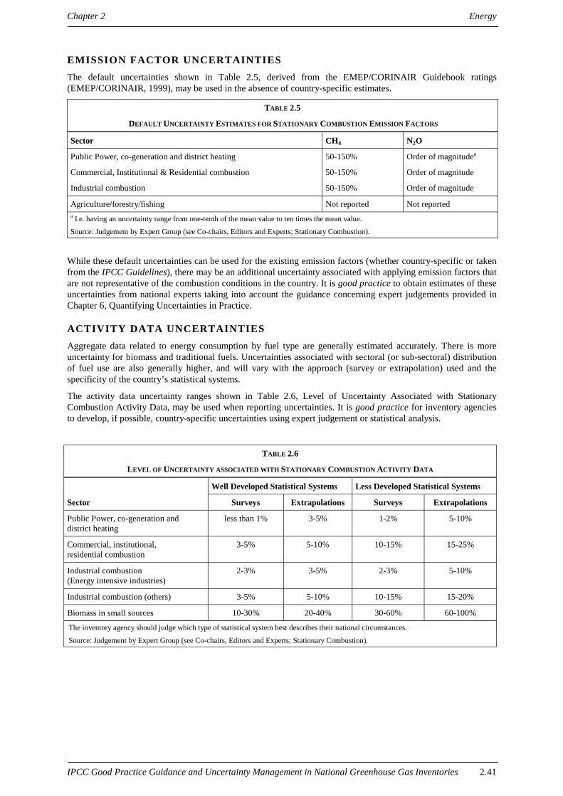
Chapter 2 Energy
IPCC Good Practice Guidance and Uncertainty Management in National Greenhouse Gas Inventories 2.41
EMISSION FACTOR UNCERTAINTIESThe default uncertainties shown in Table 2.5, derived from the EMEP/CORINAIR Guidebook ratings(EMEP/CORINAIR, 1999), may be used in the absence of country-specific estimates.
TABLE 2.5
DEFAULT UNCERTAINTY ESTIMATES FOR STATIONARY COMBUSTION EMISSION FACTORS
Sector CH4 N2O
Public Power, co-generation and district heating
Commercial, Institutional & Residential combustion
Industrial combustion
50-150%
50-150%
50-150%
Order of magnitudea
Order of magnitude
Order of magnitude
Agriculture/forestry/fishing Not reported Not reporteda I.e. having an uncertainty range from one-tenth of the mean value to ten times the mean value.
Source: Judgement by Expert Group (see Co-chairs, Editors and Experts; Stationary Combustion).
While these default uncertainties can be used for the existing emission factors (whether country-specific or takenfrom the IPCC Guidelines), there may be an additional uncertainty associated with applying emission factors thatare not representative of the combustion conditions in the country. It is good practice to obtain estimates of theseuncertainties from national experts taking into account the guidance concerning expert judgements provided inChapter 6, Quantifying Uncertainties in Practice.
ACTIVITY DATA UNCERTAINTIESAggregate data related to energy consumption by fuel type are generally estimated accurately. There is moreuncertainty for biomass and traditional fuels. Uncertainties associated with sectoral (or sub-sectoral) distributionof fuel use are also generally higher, and will vary with the approach (survey or extrapolation) used and thespecificity of the country’s statistical systems.
The activity data uncertainty ranges shown in Table 2.6, Level of Uncertainty Associated with StationaryCombustion Activity Data, may be used when reporting uncertainties. It is good practice for inventory agenciesto develop, if possible, country-specific uncertainties using expert judgement or statistical analysis.
TABLE 2.6
LEVEL OF UNCERTAINTY ASSOCIATED WITH STATIONARY COMBUSTION ACTIVITY DATA
Well Developed Statistical Systems Less Developed Statistical Systems
Sector Surveys Extrapolations Surveys Extrapolations
Public Power, co-generation anddistrict heating
less than 1% 3-5% 1-2% 5-10%
Commercial, institutional,residential combustion
3-5% 5-10% 10-15% 15-25%
Industrial combustion(Energy intensive industries)
2-3% 3-5% 2-3% 5-10%
Industrial combustion (others) 3-5% 5-10% 10-15% 15-20%
Biomass in small sources 10-30% 20-40% 30-60% 60-100%
The inventory agency should judge which type of statistical system best describes their national circumstances.
Source: Judgement by Expert Group (see Co-chairs, Editors and Experts; Stationary Combustion).

Energy Chapter 2
2.42 IPCC Good Practice Guidance and Uncertainty Management in National Greenhouse Gas Inventories
2 . 2 . 2 R e p o r t i n g a n d d o c u me n t a t i o nIt is good practice to document and archive all information required to produce the national emissions inventoryestimates as outlined in Section 8.10.1 of Chapter 8, Quality Assurance and Quality Control.
It is not practical to include all documentation in the national inventory report. However, the inventory shouldinclude summaries of methods used and references to source data such that the reported emissions estimates aretransparent and the steps in their calculation may be retraced.
The current IPCC reporting format (spreadsheet tables, aggregate tables) provides a balance between thetransparency requirement and the level of effort that is realistically achievable by the inventory agency. Goodpractice involves some additional effort to fulfil the transparency requirements completely. In particular, if Tier 2(or a more disaggregated approach) is used, additional tables showing the activity data that are directly associatedwith the emission factors should be prepared.
Most energy statistics are not considered confidential. If inventory agencies do not report disaggregated data dueto confidentiality concerns, it is good practice to explain the reasons for these concerns, and report the data in amore aggregated form.
For a highly disaggregated stationary non-CO2 estimate, it may be necessary to cite many different references ordocuments. It is good practice to provide citations for these references, particularly if they describe newmethodological developments or emission factors for particular technologies or national circumstances.
It is good practice to state clearly whether non-CO2 emissions from coke (or other fuels) used in crude ironproduction have been allocated to the Energy or to the Industrial Processes Sector, to show that no doublecounting has occurred. The attribution of emissions from blast furnaces and other industrial processes should beconsistent between CO2 and non-CO2 emissions (see Section 2.1.1.4).
2 . 2 . 3 I n v e n t o r y q u a l i t y a s s u r a n c e / q u a l i t y c o n t r o l( Q A / Q C )
It is good practice to conduct quality control checks as outlined in Chapter 8, Quality Assurance and QualityControl, Table 8.1, Tier 1 General Inventory Level QC Procedures, and expert review of the emission estimates.Additional quality control checks as outlined in Tier 2 procedures in Chapter 8 and quality assurance proceduresmay also be applicable, particularly if higher tier methods are used to determine emissions from this sourcecategory. Inventory agencies are encouraged to use higher tier QA/QC for key source categories as identified inChapter 7, Methodological Choice and Recalculation.
In addition to the guidance in Chapter 8, specific procedures of relevance to this source category are outlinedbelow.
Comparison of emission est imates using different approaches• If a Tier 2 approach with country-specific factors is used, the inventory agency should compare the result to
emissions calculated using the Tier 1 approach with default IPCC factors. This type of comparison mayrequire aggregating Tier 2 emissions to the same sector and fuel groupings as the Tier 1 approach. Theapproach should be documented and any discrepancies investigated.
• If possible, the inventory agency should compare the consistency of the calculations in relation to themaximum carbon content of fuels that are combusted by stationary sources. Anticipated carbon balancesshould be maintained throughout the combustion sectors, and the non-CO2 estimates should not contradictmaximum theoretical quantities based on the total carbon content of the fuels.
Review of emission factors• If country-specific emission factors are used, the inventory agency should compare them to the IPCC
defaults, and explain and document differences.
• The inventory agency should compare the emission factors used with site or plant level factors, if these areavailable. This type of comparison provides an indication of how reasonable and representative the nationalfactor is.

Chapter 2 Energy
IPCC Good Practice Guidance and Uncertainty Management in National Greenhouse Gas Inventories 2.43
Review of direct measurements• If direct measurements are used, the inventory agency should ensure that they are made according to good
measurement practices including appropriate QA/QC procedures. Direct measurements should be comparedto the results derived from using IPCC default factors.
Activity data check• The inventory agency should compare energy statistics with those provided to international organisations to
identify any inconsistencies that require explanation.
• If secondary data from national organisations are used, the inventory agency should ensure that theseorganisations have appropriate QA/QC programmes in place.
External review• The inventory agency should carry out a review involving national experts and stakeholders in the different
fields related to emissions from stationary sources, such as: energy statistics, combustion efficiencies fordifferent sectors and equipment types, fuel use and pollution controls. In developing countries, expert reviewof emissions from biomass combustion is particularly important.

Energy Chapter 2
2.44 IPCC Good Practice Guidance and Uncertainty Management in National Greenhouse Gas Inventories
2 . 3 M O B I L E C O M B U S T I O N : R O A D V E H I C L E S
2 . 3 . 1 M e t h o d o l o g i c a l i s s u e sRoad transport emits significant amounts of carbon dioxide (CO2), methane (CH4) and nitrous oxide (N2O), aswell as several other pollutants such as carbon monoxide (CO), non-methane volatile organic compounds(NMVOCs), sulfur dioxide (SO2), particulate matter (PM) and oxides of nitrate (NOx), which cause or contributeto local or regional air pollution problems. This chapter covers good practice in the development of estimates forthe direct greenhouse gases CO2, CH4 and N2O.
2.3.1.1 CHOICE OF METHOD
Emissions of CO2 are best calculated on the basis of the amount and type of fuel combusted and its carboncontent. Emissions of CH4 and N2O are more complicated to estimate accurately because emission factors dependon vehicle technology, fuel and operating characteristics. Both distance-based activity data (e.g. vehicle-kilometers travelled) and disaggregated fuel consumption may be considerably less certain than overall fuelconsumption.
Figure 2.4, Decision Tree for CO2 Emissions from Road Vehicles and Figure 2.5, Decision Tree for CH4 andN2O Emissions from Road Vehicles outline the process to calculate emissions from the Transport Sector. Twoalternative approaches can be used, one based on vehicle kilometres travelled and the other based on fuelconsumption. The inventory agency should choose the method on the basis of the existence and quality of data.Models can help ensure consistency and transparency because the calculation procedures are fixed in thesoftware. It is good practice to clearly document any modifications to standardised models.
F i g u r e 2 . 4 D e c i s i o n T r e e f o r C O 2 E m i s s i o n s f r o m R o a d V e h i c l e s
Areroad transport
fuel combustion dataavailable?
Collectfuel use
data
Arecountry-specificemission factors
available?
Estimate emissionsby using defaultemission factors
Estimate emissions byusing country-specific
emission factors
Box 1
No
Yes
Yes
No
Box 2

Chapter 2 Energy
IPCC Good Practice Guidance and Uncertainty Management in National Greenhouse Gas Inventories 2.45
F i g u r e 2 . 5 D e c i s i o n T r e e f o r C H 4 a n d N 2 O E m i s s i o n s f r o m R o a dV e h i c l e s
.
Isthere a
well-documentednationalmethod?
Estimateemissions usingnational method
Arefuel data
available by fueland vehicle
type?
Is this akey sourcecategory?(Note 1)
Estimate emissions byusing the
Tier 1 method
Allocateconsumption ofeach fuel type todifferent vehicle
Collectinformation on
fuel consumptionand vehicle types
Are pollutioncontrol technology data
available for eachvehicle type?
Collect information on the typeof pollution control technologiesused and estimate percentage in
total fleet
Is itpossible to estimate
vehicle km travelled bytechnology
type?
Is itpossible to estimatefuel consumption by
technologytype?
Apportion fuel use tocontrol technologies using
vehicle registrationnumbers
Allocate consumptionof each fuel type to
different vehiclecontrol technologies
Estimate emissionsusing fuel-basedemission factors
Estimate emissionsusing fuel-basedemission factors
Estimate emissions using vehiclekm based emission factors(e.g. COPERT, MOBILE)
(Tier 3)
Box 4
No
YesBox 3
Box 5
Box 2
Box 1
YesYes
Yes Yes
Yes
No
No No
No
No
Yes
Note 1: A key source category is one that is prioritised within the national inventory system because its estimate has a significantinfluence on a country’s total inventory of direct greenhouse gases in terms of the absolute level of emissions, the trend in emissions, orboth. (See Chapter 7, Methodological Choice and Recalculation, Section 7.2, Determining National Key Source Categories.)
Note 2: The decision tree and key source category determination should be applied to methane and nitrous oxide emissions separately.

Energy Chapter 2
2.46 IPCC Good Practice Guidance and Uncertainty Management in National Greenhouse Gas Inventories
CO2 EMISSIONSThe IPCC Guidelines provide two methods to estimate CO2 emissions from Road Transport. The Tier 1, or ‘topdown’ approach calculates CO2 emissions by estimating fuel consumption in a common energy unit, multiplyingby an emission factor to compute carbon content, computing the carbon stored, correcting for unoxidised carbonand finally converting oxidised carbon to CO2 emissions. The approach is shown in Equation 2.4.
EQUATION 2.4
Emissions = Σj [(Emission Factor j • Fuel consumedj) – Carbon Stored]
• Fraction Oxidisedj • 44/12
Where j = fuel type
Alternatively, a Tier 2, or ‘bottom-up’ approach estimates emissions in two steps. The first step (Equation 2.5) isto estimate fuel consumed by vehicle type i and fuel type j.
EQUATION 2.5Fuel Consumptionij = nij • kij • eij
Where:
i = vehicle type
j = fuel type
n = number of vehicles
k = annual kilometres travelled per vehicle
e = average litres consumed per kilometre travelled
The second step is to estimate total CO2 emissions by multiplying fuel consumption by an appropriate emissionfactor for the fuel type and vehicle type (Equation 2.6).
EQUATION 2.6
Emissions = ΣiΣj (Emission Factorij • Fuel Consumptionij)
It is good practice to calculate CO2 emissions on the basis of fuel consumption statistics using the Tier 1 (topdown) approach. This is illustrated in the decision tree in Figure 2.4, Decision Tree for CO2 Emissions fromRoad Vehicles. Except in rare cases (e.g. where there is extensive fuel smuggling), the top-down approach ismore reliable for CO2 estimates and is also much simpler to implement. The main issue is to ensure that doublecounting of agricultural and off-road vehicles is avoided.
It is also good practice to use the Tier 2 (bottom up) approach in parallel for the following reasons:
• First, use of these two approaches provides an important quality check. Significant differences between theresults of the top-down and bottom-up approaches indicate that one or both approaches may have errors, andthere is a need for further analysis. Areas of investigation to pursue when reconciling top down and bottom-up approaches are listed in Section 2.3.3, Inventory quality assurance/quality control (QA/QC).
• Second, a reliable and accurate bottom-up CO2 emissions estimate increases confidence in the underlyingactivity data used for the bottom-up inventory. These in turn are important underpinnings for the ‘bottom-up’calculation of CH4 and N2O emissions from road transport.
When calculating emissions using both the top-down and bottom-up approaches in parallel, it is good practice,where feasible, to develop the bottom-up estimates independently from the top-down estimates.
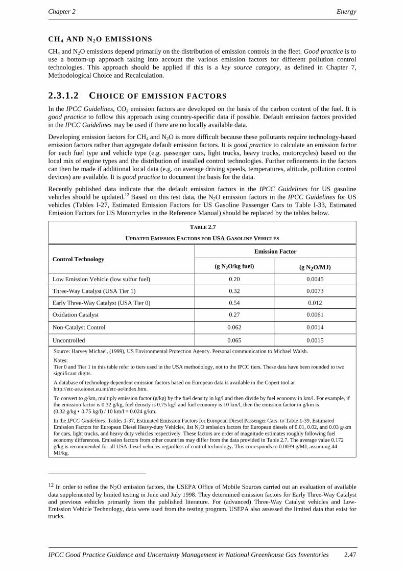
Chapter 2 Energy
IPCC Good Practice Guidance and Uncertainty Management in National Greenhouse Gas Inventories 2.47
CH4 AND N2O EMISSIONSCH4 and N2O emissions depend primarily on the distribution of emission controls in the fleet. Good practice is touse a bottom-up approach taking into account the various emission factors for different pollution controltechnologies. This approach should be applied if this is a key source category, as defined in Chapter 7,Methodological Choice and Recalculation.
2.3.1.2 CHOICE OF EMISSION FACTORS
In the IPCC Guidelines, CO2 emission factors are developed on the basis of the carbon content of the fuel. It isgood practice to follow this approach using country-specific data if possible. Default emission factors providedin the IPCC Guidelines may be used if there are no locally available data.
Developing emission factors for CH4 and N2O is more difficult because these pollutants require technology-basedemission factors rather than aggregate default emission factors. It is good practice to calculate an emission factorfor each fuel type and vehicle type (e.g. passenger cars, light trucks, heavy trucks, motorcycles) based on thelocal mix of engine types and the distribution of installed control technologies. Further refinements in the factorscan then be made if additional local data (e.g. on average driving speeds, temperatures, altitude, pollution controldevices) are available. It is good practice to document the basis for the data.
Recently published data indicate that the default emission factors in the IPCC Guidelines for US gasolinevehicles should be updated.12 Based on this test data, the N2O emission factors in the IPCC Guidelines for USvehicles (Tables I-27, Estimated Emission Factors for US Gasoline Passenger Cars to Table I-33, EstimatedEmission Factors for US Motorcycles in the Reference Manual) should be replaced by the tables below.
TABLE 2.7
UPDATED EMISSION FACTORS FOR USA GASOLINE VEHICLES
Emission FactorControl Technology
(g N2O/kg fuel) (g N2O/MJ)
Low Emission Vehicle (low sulfur fuel) 0.20 0.0045
Three-Way Catalyst (USA Tier 1) 0.32 0.0073
Early Three-Way Catalyst (USA Tier 0) 0.54 0.012
Oxidation Catalyst 0.27 0.0061
Non-Catalyst Control 0.062 0.0014
Uncontrolled 0.065 0.0015
Source: Harvey Michael, (1999), US Environmental Protection Agency. Personal communication to Michael Walsh.
Notes:Tier 0 and Tier 1 in this table refer to tiers used in the USA methodology, not to the IPCC tiers. These data have been rounded to twosignificant digits.
A database of technology dependent emission factors based on European data is available in the Copert tool athttp://etc-ae.eionet.eu.int/etc-ae/index.htm.
To convert to g/km, multiply emission factor (g/kg) by the fuel density in kg/l and then divide by fuel economy in km/l. For example, ifthe emission factor is 0.32 g/kg, fuel density is 0.75 kg/l and fuel economy is 10 km/l, then the emission factor in g/km is(0.32 g/kg • 0.75 kg/l) / 10 km/l = 0.024 g/km.
In the IPCC Guidelines, Tables 1-37, Estimated Emission Factors for European Diesel Passenger Cars, to Table 1-39, EstimatedEmission Factors for European Diesel Heavy-duty Vehicles, list N2O emission factors for European diesels of 0.01, 0.02, and 0.03 g/kmfor cars, light trucks, and heavy duty vehicles respectively. These factors are order of magnitude estimates roughly following fueleconomy differences. Emission factors from other countries may differ from the data provided in Table 2.7. The average value 0.172g/kg is recommended for all USA diesel vehicles regardless of control technology. This corresponds to 0.0039 g/MJ, assuming 44MJ/kg.
12 In order to refine the N2O emission factors, the USEPA Office of Mobile Sources carried out an evaluation of availabledata supplemented by limited testing in June and July 1998. They determined emission factors for Early Three-Way Catalystand previous vehicles primarily from the published literature. For (advanced) Three-Way Catalyst vehicles and Low-Emission Vehicle Technology, data were used from the testing program. USEPA also assessed the limited data that exist fortrucks.

Energy Chapter 2
2.48 IPCC Good Practice Guidance and Uncertainty Management in National Greenhouse Gas Inventories
2.3.1.3 CHOICE OF ACTIVITY DATA
The first step in estimating CO2 emissions using the top-down approach is to determine total fuel use in thetransportation sector by major fuel type. These data should be available from national energy statistics. Followingthis, several issues must be addressed, including:
• Provision of data for fuels with minor distribution such as compressed natural gas or biofuels. These datashould also be available from the national authority responsible for the energy statistics. According to theIPCC Guidelines, CO2 emissions from biofuels are reported as memo items but not included in nationaltotals. Non-CO2 emissions from biofuels should be included in national totals.
• Provision of data to distinguish between fuel use for on-road vehicles from fuel use for off-road vehicles,which are reported in different source categories in the IPCC Guidelines. Two alternatives are suggested:
(i) A bottom-up calculation of fuel used by each road vehicle type. The difference between the roadvehicle total (bottom-up) and the total transportation fuel used is ascribed to the off-road sector; or
(ii) The bottom-up calculation of fuel used by each road type is supplemented by special studies todetermine off-road fuel use. The total fuel use in the transportation sector (top-down estimate) isthen disaggregated according to each vehicle type and the off-road sector in proportion to thebottom-up estimates.
• Data for fuel that is sold for transportation uses but which then may be used for other purposes (or theopposite).
• Estimates of smuggling of fuels into or out of a country.
Some inventory agencies have or will have greater confidence in vehicle fuel consumption data by vehicle typeand technology while others prefer vehicle kilometres. Either approach is acceptable so long as the basis for theestimates is clearly documented.
If non-CO2 emissions from mobile sources are a key source category, more information is needed on factors thatinfluence emissions such as:
• Vehicle type (cars, light duty trucks, heavy duty trucks and motorcycles) distribution in fleet;
• Emission control technologies fitted to vehicle types in the fleet;
• Fleet age distribution;
• Climate;
• Altitude of operation;
• Maintenance effects.
If the distribution of fuel use by vehicle and fuel type is unknown, it should be estimated based on the number ofvehicles by type. If the number of vehicles by vehicle and fuel type is not known, it must be estimated fromnational statistics. If local data on annual kilometres travelled per vehicle and average fuel economies by vehicleand fuel type are available, they should be used.
2.3.1.4 COMPLETENESS
Lubricants should be accounted for in other emissions categories, as very little is combusted directly in thetransportation sector.
Regarding the problem of purchase and consumption of fuels in different countries (i.e. fuel in tanks that arecrossing a border) and the question of allocation, the IPCC Guidelines state: ‘Emissions from road vehiclesshould be attributed to the country where the fuel is loaded into the vehicle.’
Oxygenates and other blending agents should be carefully accounted for in making CO2 estimates, if used in largequantities. It is important that all fossil carbon is accounted for, and that carbon from biomass is reported as amemo item but not included in national CO2 totals, as required by the IPCC Guidelines.

Chapter 2 Energy
IPCC Good Practice Guidance and Uncertainty Management in National Greenhouse Gas Inventories 2.49
2.3.1.5 DEVELOPING A CONSISTENT TIME SERIES
With the use of models and updates or revisions of models, it is important that time series remain consistent.When models are revised, it is good practice to recalculate the complete time series. A consistent time series withregard to initial collection of fleet technology data could be difficult. Extrapolation, possibly supported by the useof proxy data will be necessary in this case for early years. Inventory agencies should refer to the discussionChapter 7, Methodological Choice and Recalculation, Section 7.3.2.2, Alternative Recalculation Techniques forgeneral guidance.
2.3.1.6 UNCERTAINTY ASSESSMENT
Carbon dioxide is usually responsible for over 97% of the CO2-equivalent emissions from the transportationsector.13 Expert judgement suggests that the uncertainty of the CO2 estimate is approximately ±5% , based onstudies with reliable fuel statistics.14 The primary source of uncertainty is the activity data rather than emissionfactors.
Nitrous oxide usually contributes approximately 3% to the CO2-equivalent emissions from the transportationsector. Expert judgement suggests that the uncertainty of the N2O estimate may be more than ±50% . The majorsource of uncertainty is related to the emission factors.
Methane usually contributes less than 1% of the CO2-equivalent emissions from the transportation sector. Expertsbelieve that there is an uncertainty of ±40% in the CH4 estimate. The major source of uncertainty is againemission factors.
To reduce uncertainty, a comprehensive approach is needed that reduces uncertainties of emission factors as wellas activity data, especially with regard to the bottom-up approach. By encouraging the use of locally estimateddata, inventories will improve despite the large uncertainties that may surround national data.
Chapter 6, Quantifying Uncertainties in Practice, describes how to use national empirical data and expertjudgement to estimate uncertainties, and how to combine uncertainty estimates for the inventory as a whole.
2 . 3 . 2 R e p o r t i n g a n d d o c u me n t a t i o nIt is good practice to document and archive all information required to produce the national emissions inventoryestimates as outlined in Section 8.10.1 of Chapter 8, Quality Assurance and Quality Control.
It is not practical to include all documentation in the national inventory report. However, the inventory shouldinclude summaries of methods used and references to source data such that the reported emissions estimates aretransparent and steps in their calculation may be retraced.
Confidentiality is not likely to be a major issue with regard to road emissions, although it is noted that in somecountries the military use of fuel may be kept confidential. The composition of some additives is confidential, butthis is only important if it influences greenhouse gas emissions.
2 . 3 . 3 I n v e n t o r y q u a l i t y a s s u r a n c e / q u a l i t y c o n t r o l( Q A / Q C )
It is good practice to conduct quality control checks as outlined in Chapter 8, Quality Assurance and QualityControl, Table 8.1, Tier 1 General Inventory Level QC Procedures, and expert review of the emission estimates.Additional quality control checks as outlined in Tier 2 procedures in Chapter 8 and quality assurance proceduresmay also be applicable, particularly if higher tier methods are used to determine emissions from this sourcecategory. Inventory agencies are encouraged to use higher tier QA/QC for key source categories as identified inChapter 7, Methodological Choice and Recalculation.
13 According to 1990 data for Annex I countries in the UNFCCC secretariat’s database on GHG emissions, updatedSeptember 1999.
14 The percentages cited in this section represent an informal polling of assembled experts aiming to approximate the 95%confidence interval around the central estimate.

Energy Chapter 2
2.50 IPCC Good Practice Guidance and Uncertainty Management in National Greenhouse Gas Inventories
In addition to the guidance in Chapter 8, specific procedures of relevance to this source category are outlinedbelow.
Comparison of emissions using alternative approachesFor CO2 emissions, the inventory agency should compare estimates using both the top-down and bottom-upapproaches. Any anomalies between the emission estimates should be investigated and explained. The results ofsuch comparisons should be recorded for internal documentation. Revising the following assumptions couldnarrow a detected gap between the approaches:
• Off-road/non transportation fuel uses;
• Annual average vehicle mileage;
• Vehicle fuel efficiency;
• Vehicle breakdowns by type, technology, age, etc.;
• Use of oxygenates/biofuels/other additives;
• Fuel use statistics;
• Fuel sold/used.
Review of emission factorsIf IPCC default factors are used, the inventory agency should ensure that they are applicable and relevant to thecategories. If possible, the IPCC default factors should be compared to local data to provide further indicationthat the factors are applicable.
For non-CO2 emissions, the inventory agency should ensure that the original data source for the local factors isapplicable to the category and that accuracy checks on data acquisition and calculations have been performed.Where possible, the IPCC default factors and the local factors should be compared. If the IPCC default factorswere used to estimate N2O emissions, the inventory agency should ensure that the revised emission factors inTable 2.7, Updated Emission Factors for USA Gasoline Vehicles were used in the calculation.
Activity data checkThe inventory agency should review the source of the activity data to ensure applicability and relevance to thecategory. Where possible, the inventory agency should compare the data to historical activity data or modeloutputs to look for anomalies. The inventory agency should ensure the reliability of activity data regarding fuelswith minor distribution, fuel used for other purposes, on and off-road traffic, and illegal transport of fuel in or outof the country. The inventory agency should also avoid double counting of agricultural and off-road vehicles.
External reviewThe inventory agency should perform an independent, objective review of the calculations, assumptions, anddocumentation of the emissions inventory to assess the effectiveness of the QC programme. The peer reviewshould be performed by expert(s) who are familiar with the source category and who understand the inventoryrequirements. The development of the factors for the non-CO2 emission estimates is particularly important due tothe associated uncertainty.

Chapter 2 Energy
IPCC Good Practice Guidance and Uncertainty Management in National Greenhouse Gas Inventories 2.51
2 . 4 M OB I L E C OM B U S T I ON : W A T E R - B OR N EN A V I G A T I O N
2 . 4 . 1 M e t h o d o l o g i c a l i s s u e sThis source category includes all emissions from fuels used to propel water-borne vessels, including hovercraftand hydrofoils. Water-borne navigation gives rise to emissions of carbon dioxide (CO2), methane (CH4) andnitrous oxide (N2O), as well as carbon monoxide (CO), non-methane volatile organic compounds (NMVOC),sulfur dioxide (SO2), particulate matter (PM) and oxides of nitrate (NOx). This section focuses on the directgreenhouse gases CO2, CH4, and N2O.
Parties to the UNFCCC have not made a final decision yet on the allocation to national GHG inventories ofemissions from fuels used for international aviation and from international marine bunkers. For the moment, allemissions from these fuels are to be excluded from national totals, and are to be reported separately.
2.4.1.1 CHOICE OF METHOD
The IPCC Guidelines present two methodological tiers for estimating emissions of CO2, CH4, and N2O fromwater-borne navigation. Both Tier 1 and Tier 2 rely on essentially the same analytical approach which is to applyemission factors to fuel consumption activity data. The fuel consumption data and emission factors in the Tier 1method are fuel type and mode-specific (e.g. oil used for navigation). The Tier 2 method presents a variety ofemission factors based on research in the United States and Europe, requiring varying degrees of specificity inthe classification of modes (e.g. ocean-going ships and boats), fuel type (e.g. gasoline), and even engine type(e.g. diesel). Figure 2.6, Decision Tree for Emissions from Water-borne Navigation helps in making a choicebetween the two tiers.
Good practice is to use Tier 1 for CO2, and Tier 2 for CH4 and N2O. Tier 1 for CO2 emissions is based on fuelconsumption by fuel type, the carbon content of the fuel, and the fraction of the fuel left unoxidised. Tier 2 fornon-CO2 emissions also uses fuel consumption by fuel type, but provides a variety of generic and country-specific emission factors for selected fuel, engine, and vehicle types. National approaches may also be goodpractice if they are well documented and have been peer reviewed.
Until the uncertainties in the CH4 and N2O emission factors are reduced, more detailed methods will notnecessarily reduce uncertainties in the emission estimates. Despite this limited reduction in uncertainty, however,these methods are likely to be desirable in the longer term for a number of other reasons. One reason is toharmonise with other emission inventory efforts that are more detailed. More detailed methods are also betterable to account for changes in technologies and therefore emission factors in the future. If improved engine-specific and fuel-specific emission factors become available, a historic database of disaggregated fuel use willallow the backcasting of a trend to the base year.
MILITARYThe IPCC Guidelines do not provide a distinct method for calculating military marine emissions. Emissions frommilitary marine fuel use can be estimated using the same ‘hybrid’ approach recommended for non-militaryshipping (i.e. Tier 1 approach for CO2, Tier 2 approach for CH4 and N2O). However, military marine navigationmay include unique operations, situations, and technologies without a civilian analogue (e.g. aircraft carriers,very large auxiliary power plants, and unique engine types). Therefore, inventory agencies should consultmilitary experts to determine the most appropriate emission factors.

Energy Chapter 2
2.52 IPCC Good Practice Guidance and Uncertainty Management in National Greenhouse Gas Inventories
F i g u r e 2 . 6 D e c i s i o n T r e e f o r E m i s s i o n s f r o m W a t e r - b o r n eN a v i g a t i o n
Arefuel consumption
data available by fuel typefor water-borne
navigation?
Havethe data been
allocated betweeninternational and
domestic?
Arenational carbon
content data and CH4 andN2O emission factors
available?
Is this akey sourcecategory?(Note 1)
Collect data orestimate using
proxy data
Develop allocationbased on otherinformation or
proxy data
Estimate CO2 emissionsusing IPCC default
carbon contents; estimateCH4 and N2O emissions
using IPCC defaultemission factors
Initiate datacollection
Isfuel-use data
by engine typeavailable?
Use Tier 1 with country specificcarbon contents for CO2 and
IPCC default emission factorsfor CH4 and N2O
Estimate emissions usingTier 2 with country specificcarbon content factors andengine specific CH4 and
N2O emission factors
Box 1
No
Yes
No No
No
Yes
Yes
Yes
Box 2
Box 3
No
Yes
Note 1: A key source category is one that is prioritised within the national inventory system because its estimate has a significantinfluence on a country’s total inventory of direct greenhouse gases in terms of the absolute level of emissions, the trend in emissions, orboth. (See Chapter 7, Methodological Choice and Recalculation, Section 7.2, Determining National Key Source Categories.)

Chapter 2 Energy
IPCC Good Practice Guidance and Uncertainty Management in National Greenhouse Gas Inventories 2.53
2.4.1.2 CHOICE OF EMISSION FACTORS
Carbon dioxide emission factors are based on the fuel type and carbon content as well as the fraction of fuel leftunoxidised. It is good practice to use national carbon content and fraction oxidised factors for CO2 whenavailable. Default values can also be used when no other information is available (IPCC Guidelines, Workbook,Table 1-2, Carbon Emission Factors and Table 1-4, Fraction of Carbon Oxidised).
There is limited information on the emission factors for CH4 and N2O from marine shipping. The IPCCGuidelines provide factors for the USA and the EU as well as factors developed by Lloyd’s Register (Table1-47, Estimated Emission Factors for US Non-road Mobile Sources to Table 1-49, Estimated Emission Factorsfor European Non-road Mobile Sources and Machinery, Reference Manual). Large ocean-going cargo ships aredriven primarily by large, slow speed and medium speed diesel engines and occasionally by steam and gasturbines. For CH4 and N2O emissions from large marine diesel engines consuming distillate or residual fuel oils,it is good practice to use the factors developed by Lloyd’s Register. These factors are based on the most recentand extensive set of test data. As marine shipping engines are predominantly diesel, and do not vary by country,national emission factors are not likely to yield improved emission estimates unless they are based on peerreviewed studies. For other vessels, such as recreational craft on inland waterways, national emission factorsshould be used if available. Alternatively, the IPCC default factors from Lloyds, the USA or the EU can be used.The difference in emission rates illustrates the importance of characterising fleet engine types and fuel use forregional scale emissions.
MILITARYCurrently, emission factors for N2O and CH4 for military vessels are not available. The default emission factorsfor civilian shipping should be used unless national data are available of sufficient quality, taking into account theadvice in Chapter 8, Quality Assurance and Quality Control.
2.4.1.3 CHOICE OF ACTIVITY DATA
Data on fuel consumption by fuel type and (for N2O and CH4) engine type are required to estimate emissions. Inaddition, in the current reporting procedures, emissions from domestic water-borne navigation are reportedseparately from international navigation which requires disaggregating the activity data to this level. Forconsistency, it is good practice to use similar definitions of domestic and international activities in the aviationand water-borne navigation estimates. These definitions are presented in Table 2.8, Criteria for DefiningInternational or Domestic Marine Transport, and are consistent with the IPCC Guidelines. They are moreprecise, however, in order to make them workable with respect to the sources of activity data. The definitions inTable 2.8 are independent of the nationality or flag of the carrier.
TABLE 2.8
CRITERIA FOR DEFINING INTERNATIONAL OR DOMESTIC MARINE TRANSPORT
Journey Type Domestic International
Originates and terminates in same country Yes No
Departs from one country and arrives in another No Yes
Departs in one country, makes a ‘technical’ stop in the same countrywithout dropping or picking up any passengers or freight, then departsagain to arrive in another country
No Yes
Departs in one country, stops in the same country and drops and picksup passengers or freight, then departs finally arriving in anothercountry
Domestic segment International segment
Departs in one country, stops in the same country and only picks upmore passengers or freight and then departs finally arriving in anothercountry
No Yes
Departs in one country with a destination in another country, andmakes an intermediate stop in the destination country where nopassengers or cargo are loaded
No Both segmentsinternational

Energy Chapter 2
2.54 IPCC Good Practice Guidance and Uncertainty Management in National Greenhouse Gas Inventories
Fuel use data may be obtained using several approaches. The most feasible approach will depend on the nationalcircumstances, but some of the options provide more accurate results than others. Several likely sources of actualfuel or proxy data are listed below, in order of typically decreasing reliability:
• National energy statistics from energy or statistical agencies;
• Surveys of shipping companies;
• Surveys of fuel suppliers (e.g. quantity of marine fuels delivered to port facilities);
• Surveys of individual port and marine authorities;
• Surveys of fishing companies;
• Equipment counts, especially for small gasoline powered fishing and pleasure craft;
• Import/export records;
• Ship movement data and standard passenger and freight ferry schedules;
• Passenger counts and cargo tonnage data;
• International Maritime Organisation (IMO), engine manufacturers, or Jane's Military Ships Database.
It may be necessary to combine these data sources to get full coverage of shipping activities.
MILITARYDue to confidentiality issues (see completeness and reporting), many inventory agencies may have difficultyobtaining data for the quantity of fuel used by the military. Military activity is defined here as those activitiesusing fuel purchased by or supplied to the military authority of the country. It is good practice to apply the rulesdefining civilian national and international operations in navigation to military operations where they arecomparable. Where they are not comparable, decisions on national and international operations should beexplained. Data on military fuel use may be obtained from government military institutions or fuel suppliers. Ifdata on fuel split are unavailable, all the fuel sold for military activities should be treated as domestic.
According to Decision 2/CP3 of the Conference of the Parties (COP), multilateral operations should not beincluded in national totals but reported separately, although there is no clear operational definition of‘multilateral operation’ available at this time.
2.4.1.4 COMPLETENESS
For water-borne navigation emissions, the methods are based on total fuel use. Since countries generally haveeffective accounting systems to measure total fuel consumption, the largest area of possible incomplete coverageof this source category is likely to be associated with misallocation of navigation emissions in another sourcecategory. For instance, for small watercraft powered by gasoline engines, it may be difficult to obtain completefuel use records and some of the emissions may be reported as industrial (when industrial companies use smallwatercraft), other off-road mobile or stationary power production. Estimates of water-borne emissions shouldinclude not only fuel for marine shipping, but also for passenger vessels, ferries, recreational watercraft, otherinland watercraft, and other gasoline-fuelled watercraft. Misallocation will not affect completeness of the totalCO2 emissions inventory. It will affect completeness of the total non-CO2 emissions inventory, because non-CO2emission factors differ between source categories.
Completeness may also be an issue where military data are confidential, unless military fuel use is aggregatedwith another source category.
There are additional challenges in distinguishing between domestic and international emissions. As eachcountry's data sources are unique for this category, it is not possible to formulate a general rule regarding how tomake an assignment in the absence of clear data. Good practice is to specify clearly the assumptions made so thatthe issue of completeness can be evaluated.
2.4.1.5 DEVELOPING A CONSISTENT TIME SERIES
For good practice guidance on determining base year emissions and ensuring consistency in the time series, seeChapter 7, Methodological Choice and Recalculation, Section 7.3.2.2, Alternative Recalculation Techniques. It isgood practice to determine fuel use using the same method for all years. If this is not possible, data collectionshould overlap sufficiently in order to check for consistency in the methods employed.

Chapter 2 Energy
IPCC Good Practice Guidance and Uncertainty Management in National Greenhouse Gas Inventories 2.55
If it is not possible to collect activity data for the base year (e.g. 1990), it may be appropriate to extrapolate databackwards using trends in freight and passenger kilometres, total fuel used or supplied, or import/export records.
Emissions of CH4 and N2O will depend on engine type and technology. Unless technology-specific emissionfactors have been developed, it is good practice to use the same fuel-specific set of emission factors for all years.
Mitigation activities resulting in changes in overall fuel consumption will be readily reflected in emissionestimates if actual fuel activity data are collected. Mitigation options that affect emission factors, however, canonly be captured by using engine-specific emission factors, or by developing control technology assumptions.Changes in emission factors over time should be well documented.
2.4.1.6 UNCERTAINTY ASSESSMENT
ACTIVITY DATAMuch of the uncertainty in emissions estimates is related to the difficulty of distinguishing between domestic andinternational fuel consumption. With complete survey data, the uncertainty may be low, while for estimations orincomplete surveys the uncertainties may be considerable. The uncertainty will vary widely from country tocountry and is difficult to generalise. The use of global data sets may be helpful in this area, and it is expectedthat reporting will improve for this category in the future.
EMISSION FACTORSExperts believe that CO2 emission factors for fuels are generally well determined within ±5%, as they areprimarily dependent on the carbon content of the fuel.15 The uncertainty for non-CO2 emissions, however, ismuch greater. The uncertainty of the CH4 emission factor may be as a high as a factor of two. The uncertainty ofthe N2O emission factor may be an order of magnitude (i.e. a factor of 10).
2 . 4 . 2 R e p o r t i n g a n d d o c u me n t a t i o nIt is good practice to document and archive all information required to produce the national emissions inventoryestimates as outlined in Section 8.10.1 of Chapter 8, Quality Assurance and Quality Control.
It is not practical to include all documentation in the national inventory report. However, the inventory shouldinclude summaries of methods used and references to source data such that the reported emissions estimates aretransparent and steps in their calculation may be retraced.
Some examples of specific documentation and reporting issues relevant to this source category are providedbelow.
Emissions related to water-borne navigation are reported in different categories depending on their nature. Forgood practice, the categories to use are:
• Civilian domestic activities;
• Military domestic activities;
• International bunker fuels;
• Fishing.
The IPCC Guidelines require that emissions from international navigation be reported separately from domestic,and not be included in the national total.
Emissions related to commercial fishing are not reported under water-borne navigation. These emissions are to bereported under the Agriculture/Forestry/Fishing category in the Energy sector. By definition, all fuel supplied tocommercial fishing activities in the reporting country is considered domestic, and there is no international bunkerfuel category for commercial fishing, regardless of where the fishing occurs.
Military marine emissions should be clearly specified to improve the transparency of national greenhouse gasinventories.
15 The uncertainty ranges cited in this section represent an informal polling of assembled experts aiming to approximate the95% confidence interval around the central estimate.

Energy Chapter 2
2.56 IPCC Good Practice Guidance and Uncertainty Management in National Greenhouse Gas Inventories
In addition to reporting emissions, it is good practice to provide:
• Source of fuel and other data;
• Method used to separate domestic and international navigation;
• Emission factors used and their associated references;
• Analysis of uncertainty or sensitivity of results or both to changes in input data and assumptions.
2 . 4 . 3 I n v e n t o r y q u a l i t y a s s u r a n c e / q u a l i t y c o n t r o l( Q A / Q C )
It is good practice to conduct quality control checks as outlined in Chapter 8, Quality Assurance and QualityControl, Table 8.1, Tier 1 General Inventory Level QC Procedures, and expert review of the emission estimates.Additional quality control checks as outlined in Tier 2 procedures in Chapter 8 and quality assurance proceduresmay also be applicable, particularly if higher tier methods are used to determine emissions from this sourcecategory. Inventory agencies are encouraged to use higher tier QA/QC for key source categories as identified inChapter 7, Methodological Choice and Recalculation.
In addition to the guidance in Chapter 8, specific procedures of relevance to this source category are outlinedbelow.
Comparison of emissions using alternative approachesIf possible, the inventory agency should compare estimates determined for water-borne navigation using bothTier 1 and Tier 2 approaches. The inventory agency should investigate and explain any anomaly between theemission estimates. The results of such comparisons should be recorded.
Review of emission factorsThe inventory agency should ensure that the original data source for national factors is applicable to eachcategory and that accuracy checks on data acquisition and calculations have been performed. For the IPCCdefault factors, the inventory agency should ensure that the factors are applicable and relevant to the category. Ifpossible, the IPCC default factors should be compared to national factors to provide further indication that thefactors are applicable and reasonable.
If emissions from military use were developed using data other than default factors, the inventory agency shouldcheck the accuracy of the calculations and the applicability and relevance of the data.
Check of act ivity dataThe source of the activity data should be reviewed to ensure applicability and relevance to the category. Wherepossible, the data should be compared to historical activity data or model outputs to look for anomalies. Datacould be checked with productivity indicators such as fuel per unit of marine traffic performance (freight andpassenger kilometres) compared with other countries.
In preparing the inventory estimates, the inventory agency should take steps to ensure reliability of the activitydata used to allocate emissions between domestic and international water-borne navigation and to ensure that allfuel sold in the country for water-borne navigation is accounted for in the estimates. A comparison of the activitydata should be conducted between multiple references due to the high uncertainty associated with this data.
External reviewThe inventory agency should carry out an independent, objective review of calculations, assumptions ordocumentation or both of the emissions inventory to assess the effectiveness of the QC programme. The peerreview should be performed by expert(s) who are familiar with the source category and who understand nationalgreenhouse gas inventory requirements.

Chapter 2 Energy
IPCC Good Practice Guidance and Uncertainty Management in National Greenhouse Gas Inventories 2.57
2 . 5 M O B I L E C O M B U S T I O N : A I R C R A F T
2 . 5 . 1 M e t h o d o l o g i c a l i s s u e sThe IPCC source category for civil aviation includes emissions from all civil commercial use of airplanes(international and domestic) consisting of scheduled and charter traffic for passengers and freight, including airtaxiing, as well as general aviation16 (e.g. agricultural airplanes, private jets or helicopters). Methods discussed inthis section can be used also to estimate emissions from military aviation, but emissions should be reported underthe IPCC category 1A 5 ’Other‘. Stationary combustion and ground transport at airports are to be included inother appropriate categories.
Aircraft emit carbon dioxide (CO2), methane (CH4) and nitrous oxide (N2O), as well as carbon monoxide (CO),non-methane volatile organic compounds (NMVOCs), sulfur dioxide (SO2), particulate matter (PM) and nitrogenoxides (NOx). This section focuses on the direct greenhouse gases CO2, CH4 and N2O. For more information onthe impact of aviation on the global atmosphere see IPCC (1999).
Parties to the UNFCCC have not made a final decision yet on the allocation to national GHG inventories ofemissions from fuels used for international aviation and from international marine bunkers. For the moment, allemissions from these fuels are to be excluded from national totals, and are to be reported separately.
2.5.1.1 CHOICE OF METHOD
One Tier 1 and two Tier 2 methods (designated Tier 2a and 2b) are outlined in the IPCC Guidelines. All methodsare based on distinguishing between domestic fuel use and international fuel use. Tier 1 is purely fuel based,while the Tier 2 methods are based on the number of landing/take-off cycles (LTOs) and fuel use. The CO2estimate depends on carbon content of fuel and the fraction oxidised and therefore should not vary significantlywith the tier. Given the current limited knowledge of emission factors, more detailed methods will notsignificantly reduce uncertainties for CH4 and N2O emissions. However, reasons for choosing to use a higher tierinclude estimation of emissions jointly with other pollutants (e.g. NOx), harmonisation of methods with otherinventories, and the possibility of accounting for changes in technologies (and therefore emission factors) in thefuture.
All three methods will capture changes in technology that influence fuel consumption. However, only Tier 2b cancapture the effects on CH4 and N2O emissions of changing emission factors. National approaches can also beused if they are well documented and have been peer reviewed. The choice of method will depend on nationalcircumstances particularly the availability of data (see the decision trees in Figure 2.7 and Figure 2.8).
The simple Tier 1 method is based on an aggregate figure of fuel consumption for civil aviation multiplied byaverage emissions factors. The emissions factors have been averaged over all flying phases based on theassumption that 10% of the fuel17 is used in the LTO18 (landing/take-off) phase of the flight. Emissions arecalculated according to Equation 2.7:
EQUATION 2.7Emissions = Fuel Consumption • Emission Factor
The Tier 2 method is only applicable for jet fuel use in jet engines. Aviation gasoline is only used in smallaircraft and generally represents less than 1% of fuel consumption from aviation. In the Tier 2 method a 16 ICAO’s ‘Manual on the ICAO Statistics Programme’ defines ‘general aviation’ as all civil operations other than scheduledair services and non-scheduled air transport operations for remuneration or hire. For ICAO statistical purposes, the generalaviation activities are classified into instructional flying, business and pleasure flying, aerial work and other flying.
17 Source: Olivier, 1995. This percentage will vary according to national circumstances and countries are encouraged tomake their own assessment.
18 Both a single landing together with a single take-off define one LTO operation that includes all activities near the airportthat take place under an altitude of 914 m (3000 feet): engines running idle, taxi-in and out, take-off, climbing anddescending. Aircraft operations above 914 m are defined as ‘cruise’.
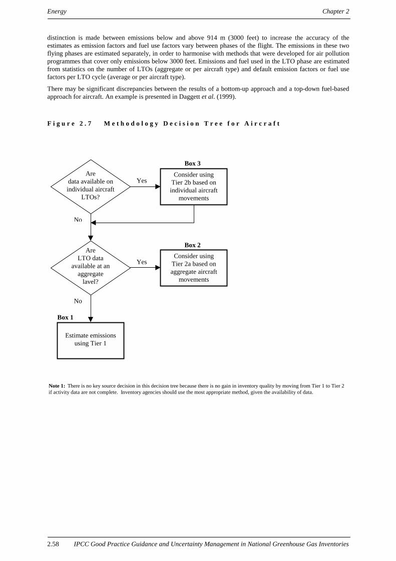
Energy Chapter 2
2.58 IPCC Good Practice Guidance and Uncertainty Management in National Greenhouse Gas Inventories
distinction is made between emissions below and above 914 m (3000 feet) to increase the accuracy of theestimates as emission factors and fuel use factors vary between phases of the flight. The emissions in these twoflying phases are estimated separately, in order to harmonise with methods that were developed for air pollutionprogrammes that cover only emissions below 3000 feet. Emissions and fuel used in the LTO phase are estimatedfrom statistics on the number of LTOs (aggregate or per aircraft type) and default emission factors or fuel usefactors per LTO cycle (average or per aircraft type).
There may be significant discrepancies between the results of a bottom-up approach and a top-down fuel-basedapproach for aircraft. An example is presented in Daggett et al. (1999).
F i g u r e 2 . 7 M e t h o d o l o g y D e c i s i o n T r e e f o r A i r c r a f t
Aredata available onindividual aircraft
LTOs?
Consider usingTier 2b based onindividual aircraft
movements
AreLTO data
available at anaggregate
lavel?
Estimate emissionsusing Tier 1
Box 1
No
Yes
Yes
No
Box 2Consider using
Tier 2a based onaggregate aircraft
movements
Box 3
Note 1: There is no key source decision in this decision tree because there is no gain in inventory quality by moving from Tier 1 to Tier 2if activity data are not complete. Inventory agencies should use the most appropriate method, given the availability of data.

Chapter 2 Energy
IPCC Good Practice Guidance and Uncertainty Management in National Greenhouse Gas Inventories 2.59
F i g u r e 2 . 8 A c t i v i t y D a t a D e c i s i o n T r e e f o r A i r c r a f t
Aretotal nationalfuel statistics
available?
No
Yes
Is itfeasible to
survey airports or fuelsuppliers?
Initiate datacollection
Do thenational fuel
statistics differentiatebetween domestic and
international fuel use, or is it possibleto survey licensed airlines on
their domestic versusinternational
fuel use?
Is itpossible to estimate
domestic/internationalfuel use based on LTO data per
aircraft type anddistance/time
travelled?
Initiate work on datacollection.
Ensure that CO2emissions are
calculated using theReference Approach
Estimate fuel consumption andcalculate ratio between
domestic and international fueluse. Correct for other uses:
subtract total for stationary use,add fuel for general aviation.
Verify the data and usefor emission estimation.
Estimate fuel consumption andcalculate ratio between
domestic and international fueluse. Correct for other uses:
subtract total for stationary use,add fuel for general aviation.
Verify the data and usefor emission estimation.
No
Yes
No
Yes
No
Yes
Box 1Box 2
Box 3

Energy Chapter 2
2.60 IPCC Good Practice Guidance and Uncertainty Management in National Greenhouse Gas Inventories
Both Tier 2 approaches use Equations 2.8 to 2.11 to estimate emissions:
EQUATION 2.8Emissions = LTO Emissions + Cruise Emissions
Where
EQUATION 2.9LTO Emissions = Number of LTOs • Emission FactorLTO
EQUATION 2.10LTO Fuel Consumption = Number of LTOs • Fuel Consumption per LTO
EQUATION 2.11Cruise Emissions = (Total Fuel Consumption – LTO Fuel Consumption) • Emission FactorCRUISE
These equations can be applied at either the aggregated level of all aircraft (Tier 2a) or at the level of individualaircraft types (Tier 2b). For the Tier 2b approach, the estimate should include all aircraft types frequently usedfor domestic and international aviation. For the Tier 2a approach, all aircraft are included and the IPCCGuidelines provide aggregate emission factors per LTO. The aggregated emission factors are proposed fornational and international aviation separately, and for an old and average fleet.
Cruise emissions depend on the length of the flight among other variables. In the Tier 2 method the fuel used inthe cruise phase is estimated as total fuel use minus fuel used in the LTO phase of the flight as shown inEquation 2.11. Fuel use is estimated for domestic and international aviation separately. The estimated fuel use ismultiplied by aggregate emission factors (average or per aircraft type) in order to estimate the emissions.
The resource demand for the various tiers depends on the number of air traffic movements and the availability ofthe data in the country. Tier 1 and Tier 2a, based on aggregate LTO data, should not require considerableresources, while Tier 2b, based on individual aircraft, may be very time consuming.
2.5.1.2 CHOICE OF EMISSION FACTORS
It is good practice to use emission factors from the IPCC Guidelines. National emission factors for CO2 shouldnot deviate much from the default values because the quality of jet fuel is well defined. However, there is limitedinformation on the emission factors for CH4 and N2O from aircraft, and the IPCC default values are similar tovalues found in the literature. Since aircraft technologies do not vary by country, national emission factors shouldgenerally not be used unless based on peer reviewed studies.
Within this sector, different types of aircraft/engine combinations have specific emission factors and these factorsmay also vary according to distance flown. It has been assumed that all aircraft have the same emission factorsfor CH4 and N2O based on the rate of fuel consumption. This assumption has been made because moredisaggregated emission factors are not available.
MILITARYEmissions from military aviation may be estimated by the Tier 1 approach (total fuel use and average emissionfactors). However, the term ‘military aircraft’ covers very different technologies (e.g. transport planes,helicopters and fighters) and the use of a more detailed method is encouraged if data are available. No emissionfactors for N2O and CH4 have been developed for military aviation. However, many types of military transportaircraft and helicopters have fuel and emissions characteristics similar to civil types. The default emission factorsfor civil aircraft should be used for military aviation unless better data are available. For fuel use factors see‘Choice of activity data’ below.

Chapter 2 Energy
IPCC Good Practice Guidance and Uncertainty Management in National Greenhouse Gas Inventories 2.61
2.5.1.3 CHOICE OF ACTIVITY DATA
According to the IPCC Guidelines, emissions from domestic aviation are reported separately from internationalaviation. For this reason, it is necessary to disaggregate fuel use into domestic and international components.Table 2.9, Distinction between Domestic and International Flights presents good practice in flight classification.These definitions are a precision of the ones given the IPCC Guidelines. These definitions should be appliedirrespective of the nationality of the carrier.19
TABLE 2.9
DISTINCTION BETWEEN DOMESTIC AND INTERNATIONAL FLIGHTS
Domestic International
Depart and arrive in same country Yes No
Depart from one country and arrive in another No Yes
Depart in one country, stop in the same country without dropping orpicking up any passengers or freight, then depart again to arrive inanother country
No Yes
Depart in one country, stop in the same country and drop and pick uppassengers or freight, then depart finally arriving in another country
Domestic stage International stage
Depart in one country, stop in the same country, only pick up morepassengers or freight and then depart finally arriving in anothercountry
No Yes
Departs in one country with a destination in another country, andmakes an intermediate stop in the destination country where nopassengers or cargo are loaded.
No Both segmentsinternational
For consistency, it is good practice to use similar definitions of domestic and international activities in theaviation and water-borne navigation estimates.
Fuel use data distinguished between domestic and international aviation may be obtained in different ways. Whatis feasible will depend on national circumstances, but some data sources (e.g. energy statistics or surveys) willgive more accurate results than others. The following data sources should be evaluated:
Bottom-up data can be obtained from surveys of airline companies for fuel used, or estimates from aircraftmovement data and standard tables of fuel consumed or both.
Top-down data can be obtained from national energy statistics or surveys of:
• Airports for data covering the delivery of aviation kerosene and aviation gasoline;
• Fuel suppliers (quantity of aviation fuel delivered);
• Refineries (production of aviation fuels), to be corrected for import and export.
Fuel consumption factors for aircraft (fuel used per LTO and per nautical mile cruised) can be used for estimatesand may be obtained from the airline companies. Table 2.10, Fuel Use and Average Sector Distance forRepresentative Types of Aircraft, shown in Appendix 2.5A.1 shows the data derived for the sixteen aircraft typesused to represent the world's commercial passenger fleet in the ANCAT/EC2 global inventory20 (ANCAT/EC2,1998) plus three aircraft which subsequently came into revenue service (Falk, 1999). Similar data could be 19 The treatment of domestic and international aviation, both in the IPCC Guidelines and in Table 2.9 above, differs fromthat recommended to states by the International Civil Aviation Organization for the purposes of classifying flight stages whenreporting air carrier statistical data (ICAO, 1997). In this context, ICAO defines as domestic, all flight stages flown betweendomestic points by an air carrier whose principal place of business is in that state and therefore (i) includes flight stagesbetween domestic points that precede a flight stage to another country, and (ii) excludes flights between domestic points byforeign carriers.
20 The ANCAT/EC2 global inventory was a programme that was part-funded by the EC to produce a world-wide 3D griddedinventory of fuel used and NOx produced from civil commercial and bizjet aircraft, cargo planes and military operations. Thebase year was 1991/92 and the forecast year was 2015. The data were gridded into 1o • 1o • 1 km boxes by summingindividual movements. The results of the ANCAT/EC2 and NASA inventories were similar to each other.

Energy Chapter 2
2.62 IPCC Good Practice Guidance and Uncertainty Management in National Greenhouse Gas Inventories
obtained from other sources (e.g. EMEP/CORINAIR inventory guidebook, second edition, 1999). The equivalentdata for turboprop and piston engine aircraft need to be obtained from other sources. The relationship betweenactual aircraft and representative aircraft is shown in Table 2.11, Correspondence between RepresentativeAircraft and Other Aircraft Types in Appendix 2.5A.2.
Aircraft movement data may be obtained from:
• Statistical offices or transport ministries as a part of national statistics;
• Airport records;
• ATC (Air Traffic Control) records, for example EUROCONTROL statistics;
• OAG (Official Airline Guide), published by Reed Publishing (monthly) which contains timetable passengerand freight movements, but does not contain non-scheduled traffic (e.g. passenger charter and non-scheduledfreight operations);
• Passenger numbers and cargo tonnage data (these are not very reliable because of variations in load factorand type of aircraft used).
Note that some of these sources do not cover all flights (e.g. charter flights may be excluded). On the other hand,airline guide data may count some flights more than once (Baughcum et al., 1996). Whatever data source is used,inventory agencies must assure completeness. If fuel data for domestic aviation are not readily available, bothdata collection and estimation will usually be time consuming to perform.
MILITARYDue to confidentiality concerns, it may be difficult to obtain data covering the quantity of fuel used by themilitary. This will have consequences for transparency and possibly completeness. Military activity is defined asthose activities for which aviation fuel has been purchased by, or supplied to, the military authority of thecountry. It is good practice to apply the rules defining civilian national and international operations in aviation tomilitary operations where they are comparable. Where they are not comparable, it is good practice to explaindecisions on national and international operations. Unless better information is available, all the fuel should beallocated as domestic. Data on military fuel use may be sought from the military authorities themselves and thefuel suppliers.
The IPCC Guidelines do not provide a method to assess the quantity of fuel from military aviation althoughmilitary fuel use should be available from national data sources. An estimate of fuel used for military aviation isgiven in ANCAT/EC2 (1998) (transport and tanker, fighter/bomber and light aircraft/helicopters) together withthe method used to obtain it. Methods for estimating CH4 and N2O emissions are not included.
Alternatively, fuel use may be estimated from the hours in operation. Default fuel consumption factors are givenin Table 2.12, Fuel Consumption Factors for Military Aircraft shown in Appendix 2.5A.3.
According to COP Decision 2/CP3 a multilateral operation should not be included in national totals but reportedseparately, although there is no clear operational definition of ‘multilateral operation’ available at this time.
2.5.1.4 COMPLETENESS
Regardless of method, it is important to account for all fuel sold for aviation in the country. The methods arebased on total fuel use, and should completely cover CO2 emissions. However, the Tier 2 methods focus onpassenger and freight carrying scheduled and charter flights, and not all aviation. In addition, they do notautomatically include non-scheduled flights and general aviation such as agricultural airplanes, private jets orhelicopters, which should be added if the quantity of fuel is significant. Completeness may also be an issue wheremilitary data are confidential, unless military fuel use is aggregated with another source category.
2.5.1.5 DEVELOPING A CONSISTENT TIME SERIES
Chapter 7, Methodological Choice and Recalculation, Section 7.3.2.2, Alternative Recalculation Techniquesprovides more information on how to develop emission estimates in cases where the same data sets or methodscannot be used during every year of the time series. If activity data are unavailable for the base year (e.g. 1990)an option may be to extrapolate data to this year by using changes in freight and passenger kilometres, total fuelused or supplied, or the number of LTOs (aircraft movements).
Emissions trends of CH4 and NOx (and by inference N2O) will depend on aircraft engine technology and thechange in composition of a country's fleet. This change in fleet composition may have to be accounted for in the

Chapter 2 Energy
IPCC Good Practice Guidance and Uncertainty Management in National Greenhouse Gas Inventories 2.63
future, and this is best accomplished using the Tier 2b method based on individual aircraft types for 1990 andsubsequent years. If fleet composition is not changing, the same set of emission factors should be used for allyears.
Every method should be able to reflect accurately the results of mitigation options that lead to changes in fueluse. Only the Tier 2b method, based on individual aircraft, can capture the effect of mitigation options that resultin lower emission factors.
2.5.1.6 UNCERTAINTY ASSESSMENT
ACTIVITY DATAThe uncertainty in the reporting will be strongly influenced by the accuracy of the data collected on domesticaviation separately from international aviation. With complete survey data, the uncertainty may be very low (lessthan 5%) while for estimates or incomplete surveys the uncertainties may become large, perhaps a factor of twofor the domestic share.21
EMISSION FACTORSThe CO2 emission factors should be within a range of ±5%, as they are dependent only on the carbon content ofthe fuel and fraction oxidised. The uncertainty of the CH4 emission factor may be as a high as a factor of 2. Theuncertainty of the N2O emission factor may be of several orders of magnitude (i.e. a factor of 10, 100 or more).
2 . 5 . 2 R e p o r t i n g a n d d o c u me n t a t i o nIt is good practice to document and archive all information required to produce the national emissions inventoryestimates as outlined in Section 8.10.1 of Chapter 8, Quality Assurance and Quality Control.
It is not practical to include all documentation in the national inventory report. However, the inventory shouldinclude summaries of methods used and references to source data such that the reported emissions estimates aretransparent and steps in their calculation may be retraced.
Some examples of specific documentation and reporting relevant to this source category are provided below.
The IPCC Guidelines require that inventory agencies report emissions from international aviation separatelyfrom domestic aviation, and exclude international aviation from national totals. It is expected that all countrieshave aviation activity and should therefore report emissions from this category. Though countries covering smallareas might not have domestic aviation, emissions from international aviation should be reported.
Transparency would be improved if inventory agencies report emissions from LTO separately from cruiseoperations (defined here as operations above 3000 feet or 914 m).
Emissions from military aviation should be clearly specified, so as to improve the transparency on nationalgreenhouse gas inventories.
In addition to the standard reporting required in the IPCC Guidelines, provision of the following data wouldincrease transparency:
• Sources of fuel data and other essential data (e.g. fuel consumption factors) depending on the method used;
• The number of flight movements split between domestic and international;
• Emission factors used, if different from default values. Data sources should be referenced.
Inventory agencies should provide the definition of international and domestic that has been used and documentwhy and how it was applied.
Confidentiality may be a problem if only one or two airline companies operate domestic transport in a givencountry. Confidentiality may also be a problem for reporting military aviation in a transparent manner.
21 The uncertainty ranges cited in this section represent an informal polling of assembled experts aiming to approximate the95% confidence interval around the central estimate.

Energy Chapter 2
2.64 IPCC Good Practice Guidance and Uncertainty Management in National Greenhouse Gas Inventories
2 . 5 . 3 I n v e n t o r y q u a l i t y a s s u r a n c e / q u a l i t y c o n t r o l( Q A / Q C )
It is good practice to conduct quality control checks as outlined in Chapter 8, Quality Assurance and QualityControl, Table 8.1, Tier 1 General Inventory Level QC Procedures, and expert review of the emission estimates.Additional quality control checks as outlined in Tier 2 procedures in Chapter 8 and quality assurance proceduresmay also be applicable, particularly if higher tier methods are used to determine emissions from this sourcecategory. Inventory agencies are encouraged to use higher tier QA/QC for key source categories as identified inChapter 7, Methodological Choice and Recalculation.
In addition to the guidance in Chapter 8, specific procedures of relevance to this source category are outlinedbelow.
Comparison of emissions using alternative approachesThe inventory agency should compare the emission estimates for aircraft using both Tier 1 and Tier 2approaches. Any anomaly between the emission estimates should be investigated and explained. The results ofsuch comparisons should be recorded for internal documentation.
Review of Emission factorsIf national factors are used rather than the default values, directly reference the QC review associated with thepublication of the emission factors, and include this review in the QA/QC documentation to ensure that theprocedures are consistent with good practice. If possible, the inventory agency should compare the IPCC defaultvalues to national factors to provide further indication that the factors are applicable. If emissions from militaryuse were developed using data other than the default factors, the accuracy of the calculations and the applicabilityand relevance of the data should be checked.
Activity data checkThe source of the activity data should be reviewed to ensure applicability and relevance to the source category.Where possible, the inventory agency should compare current data to historical activity data or model outputs tolook for anomalies. In preparing the inventory estimates, the inventory agency should ensure the reliability of theactivity data used to allocate emissions between domestic and international aviation.
Data could be checked with productivity indicators such as fuel per unit of traffic performance (per passenger kmor ton km). Where data from different countries are being compared, the band of data should be small.
External reviewThe inventory agency should perform an independent, objective review of calculations, assumptions ordocumentation of the emissions inventory to assess the effectiveness of the QC programme. The peer reviewshould be performed by expert(s) (e.g. aviation authorities, airline companies, and military staff) who are familiarwith the source category and who understand inventory requirements.
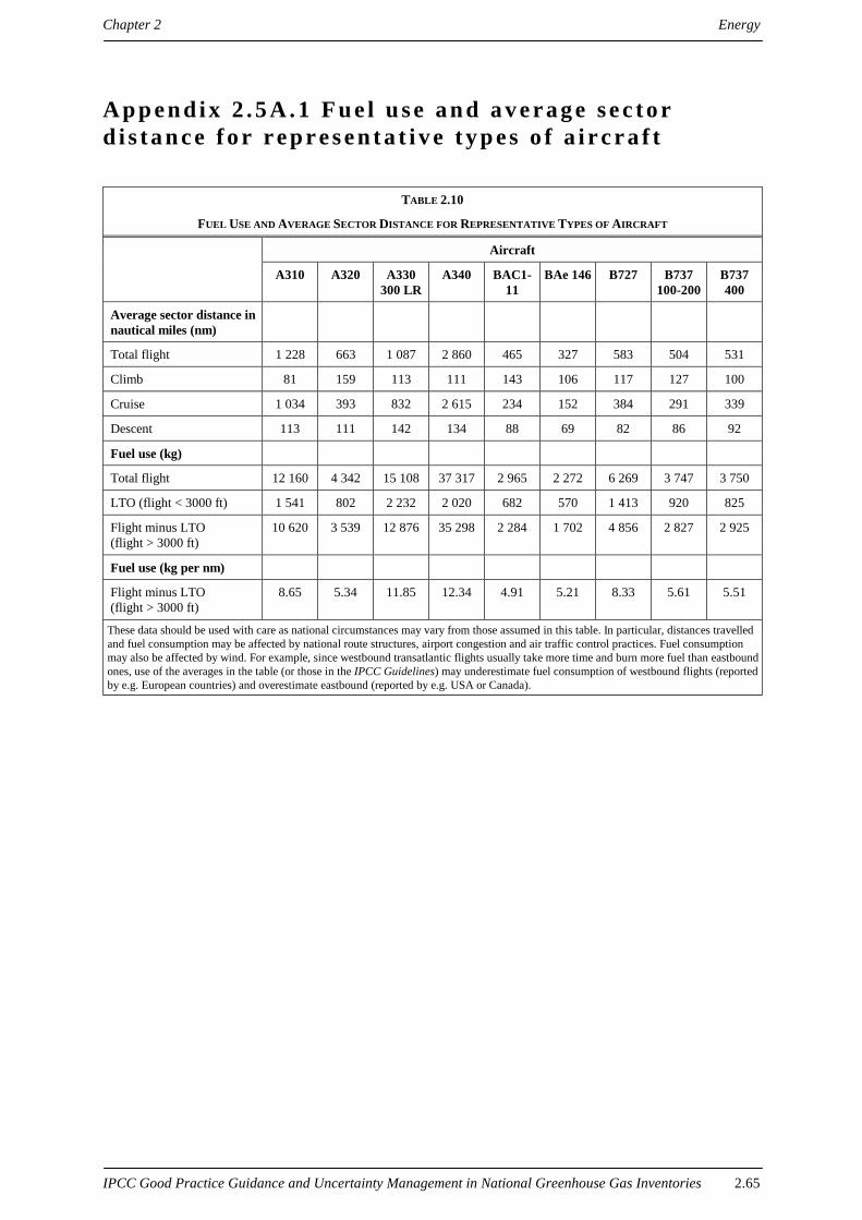
Chapter 2 Energy
IPCC Good Practice Guidance and Uncertainty Management in National Greenhouse Gas Inventories 2.65
A p p e n d i x 2 . 5 A . 1 F u e l u s e a n d a v e r a g e s e c t o rd i s t a n c e f o r r e p r e s e n t a t i v e t y p e s o f a i r c r a f t
TABLE 2.10
FUEL USE AND AVERAGE SECTOR DISTANCE FOR REPRESENTATIVE TYPES OF AIRCRAFT
Aircraft
A310 A320 A330300 LR
A340 BAC1-11
BAe 146 B727 B737100-200
B737400
Average sector distance innautical miles (nm)
Total flight 1 228 663 1 087 2 860 465 327 583 504 531
Climb 81 159 113 111 143 106 117 127 100
Cruise 1 034 393 832 2 615 234 152 384 291 339
Descent 113 111 142 134 88 69 82 86 92
Fuel use (kg)
Total flight 12 160 4 342 15 108 37 317 2 965 2 272 6 269 3 747 3 750
LTO (flight < 3000 ft) 1 541 802 2 232 2 020 682 570 1 413 920 825
Flight minus LTO(flight > 3000 ft)
10 620 3 539 12 876 35 298 2 284 1 702 4 856 2 827 2 925
Fuel use (kg per nm)
Flight minus LTO(flight > 3000 ft)
8.65 5.34 11.85 12.34 4.91 5.21 8.33 5.61 5.51
These data should be used with care as national circumstances may vary from those assumed in this table. In particular, distances travelledand fuel consumption may be affected by national route structures, airport congestion and air traffic control practices. Fuel consumptionmay also be affected by wind. For example, since westbound transatlantic flights usually take more time and burn more fuel than eastboundones, use of the averages in the table (or those in the IPCC Guidelines) may underestimate fuel consumption of westbound flights (reportedby e.g. European countries) and overestimate eastbound (reported by e.g. USA or Canada).

Energy Chapter 2
2.66 IPCC Good Practice Guidance and Uncertainty Management in National Greenhouse Gas Inventories
TABLE 2.10 (CONTINUED)
FUEL USE AND AVERAGE SECTOR DISTANCE FOR REPRESENTATIVE TYPES OF AIRCRAFT
Aircraft
B747100-300
B747400
B757 B767300 ER
B777 F28 F100 DC9 DC10-30
MD82-88
Average sector distance innautical miles (nm)
Total flight 2 741 2 938 958 1 434 1 579 295 360 384 2 118 557
Climb 152 95 106 100 112 131 118 118 117 161
Cruise 2 480 2 727 744 1 205 1 325 91 158 182 1 902 306
Descent 109 116 108 129 141 73 84 84 99 90
Fuel use (kg)
Total flight 60 705 58 325 8 111 14 806 23 627 2 104 2 597 3 202 35 171 4 872
LTO (flight < 3000 ft) 3 414 3 402 1 253 1 617 2 563 666 744 876 2 381 1 003
Flight minus LTO (flight >3000 ft)
57 291 54 923 6 858 13 189 21 064 1 438 1 853 2 326 32 790 3 869
Fuel use (kg per nm)
Flight minus LTO(flight > 3000 ft)
20.90 18.69 7.16 9.20 13.34 4.87 5.15 6.06 15.48 6.95
Source: ANCAT/EC2 and UK Department of Trade and Industry (DTI/EID3cC/199803).

Chapter 2 Energy
IPCC Good Practice Guidance and Uncertainty Management in National Greenhouse Gas Inventories 2.67
A p p e n d i x 2 . 5 A . 2 C o r r e s p o n d e n c e b e t w e e nr e p r e s e n t a t i v e a i r c r a f t a n d o t h e r a i r c r a f t t y p e s
TABLE 2.11CORRESPONDENCE BETWEEN REPRESENTATIVE AIRCRAFT AND OTHER AIRCRAFT TYPES
Genericaircrafttype
ICAO IATAaircraftin group
Genericaircrafttype
ICAO IATAaircraftin group
Genericaircrafttype
ICAO IATAaircraftin group
Genericaircrafttype
ICAO IATAaircraftin group
BAe 146 BA46 141 Airbus A320 A320 320 Boeing747-400
B744 744 McDonnellDouglasDC10
DC10 D10
143 32S Boeing757
757 D11
146 321 75F D1C
14F Airbus A319 A319 319 TR2 D1F
AirbusA310
A310 310 Airbus A330 A330 330 Boeing767
762 L10
312 332 763 L11
313 333 767 L12
A31 Airbus A340 A340 340 AB3 L15
Boeing727-100
B721 721 342 AB6 M11
Boeing727-200
B722 722 343 A3E M1F
Boeing727-300
B727 727 BAe 111 BA11 B11 ABF McDonnellDouglas DC8
DC8
72A B15 AB4 D8F
72F CRV Boeing777
777 D8M
72M F23 Boeing777-200
B772 772 D8S
72S F24 Boeing777-300
B773 773 707
TU5 YK4 McDonnellDouglasDC-9
D92 70F
Boeing737-200
B732 732 Boeing 747-100-300
B741 741 D93 IL6
Boeing737-500
B735 735 B742 742 D94 B72
73A B743 743 D95
73B 747 D98
73F 74D D9S
73M 74E DC9
73S 74F F21
D86 A4F TRD
JET 74L YK2
DAM 74M McDonnellDouglasM81-88
MD81-88
M80

Energy Chapter 2
2.68 IPCC Good Practice Guidance and Uncertainty Management in National Greenhouse Gas Inventories
TABLE 2.11 (CONTINUED)CORRESPONDENCE BETWEEN REPRESENTATIVE AIRCRAFT AND OTHER AIRCRAFT TYPES
Genericaircrafttype
ICAO IATAaircraftin group
Genericaircrafttype
ICAO IATAaircraftin group
Genericaircrafttype
ICAO IATAaircraftin group
Genericaircrafttype
ICAO IATAaircraftin group
Boeing737-300
B733 733 IL7 M82
Boeing737-700
B737 737 ILW M83
Fokker100
F100 100 NIM M87
FokkerF-28
F28 F28 VCX M88
TU3 C51
MD90 goes as MD81-88 and B737-600 goes as B737-400. DC8 goes as double the B737-100.
Source: Falk (1999b) and EMEP/CORINAIR (1999).

Chapter 2 Energy
IPCC Good Practice Guidance and Uncertainty Management in National Greenhouse Gas Inventories 2.69
A p p e n d i x 2 . 5 A . 3 F u e l c o n s u mp t i o n f a c t o r s f o rmi l i t a r y a i r c r a f t
TABLE 2.12
FUEL CONSUMPTION FACTORS FOR MILITARY AIRCRAFT
Group Sub-group Representative type Fuel flow (kg/hour)
Combat Fast Jet - High Thrust
Fast Jet - Low Thrust
F16
Tiger F-5E
3 283
2 100
Trainer Jet trainers
Turboprop trainers
Hawk
PC-7
720
120
Tanker/Transport Large Tanker/Transport
Small Transport
C-130
ATP
2 225
499
Other MPAs, Maritime Patrol C-130 2 225
Source: Tables 3.1 and 3.2 of ANCAT/EC2 1998, British Aerospace/Airbus.
TABLE 2.13
ANNUAL AVERAGE FUEL CONSUMPTION PER FLIGHT HOUR FOR UNITED STATES MILITARY AIRCRAFT ENGAGED INPEACETIME TRAINING OPERATIONS
Aircraft Type Aircraft Description Fuel Use(Litres per Hour)
A-10A Twin engine light bomber 2 331
B-1B Four engine long-range strategic bomber. Used by USA only 13 959
B-52H Eight engine long-range strategic bomber. Used by USA only. 12 833
C-12J Twin turboprop light transport. Beech King Air variant. 398
C-130E Four turboprop transport. Used by many countries. 2 956
C-141B Four engine long-range transport. Used by USA only 7 849
C-5B Four engine long-range heavy transport. Used by USA only 13 473
C-9C Twin engine transport. Military variant of DC-9. 3 745
E-4B Four engine transport. Military variant of Boeing 747. 17 339
F-15D Twin engine fighter. 5 825
F-15E Twin engine fighter-bomber 6 951
F-16C Single engine fighter. Used by many countries. 3 252
KC-10A Three engine tanker. Military variant of DC-10 10 002
KC-135E Four engine tanker. Military variant of Boeing 707. 7 134
KC-135R Four engine tanker with newer engines. Boeing 707 variant. 6 064
T-37B Twin engine jet trainer. 694
T-38A Twin engine jet trainer. Similar to F-5. 262
These data should be used with care as national circumstances may vary from those assumed in this table. In particular, distancestravelled and fuel consumption may be affected by national route structures, airport congestion and air traffic control practices.
Source: US Environmental Protection Agency, Inventory of US Greenhouse Gas Emissions and Sinks, 1990-1998, EPA-236-R-00-001(Forthcoming, April 2000). Data provided by the US Department of Defense.

Energy Chapter 2
2.70 IPCC Good Practice Guidance and Uncertainty Management in National Greenhouse Gas Inventories
2 . 6 F U G I T I V E E M I S S I O N S F R O M C O A LM I N I N G A N D H A N D L I N G
2 . 6 . 1 M e t h o d o l o g i c a l i s s u e sThe geological process of coal formation also produces methane (CH4), some of which remains trapped in thecoal seam until it is mined. Generally, deeper underground coal seams contain more in-situ methane thanshallower surface seams. Consequently, the majority of emissions come from deep underground mines.Additional emissions come from open-pit mines and post-mining activities.
2.6.1.1 CHOICE OF METHOD
Those coal-mining countries whose major production is from underground mining, particularly longwalloperations, the emissions from this sub-source category will dominate and efforts should focus on this part of theoverall coal estimate. However, where there is extensive open-cut mining such as in Australia, emissions fromthis activity can also be significant. Figure 2.9, Decision Tree for Surface Coal Mining and Handling, to Figure2.11, Decision Tree for Post-mining provide guidance in choosing the appropriate method for all sources of coalmine methane. The IPCC Guidelines give the following general equation for estimating emissions:
EQUATION 2.12Emissions = Coal Production (Surface or Underground) • Emission Factor
The Tier 2 approach is to use country or basin-specific emission factors that reflect the average methane contentof coal actually mined. The Tier 1 default approach requires that countries choose from a global average range ofemission factors, and is more uncertain as a consequence. For underground mines, actual measurement data maybe available. Although not specified explicitly as Tier 3 in the coal chapter of the IPCC Guidelines, the use ofmeasurement data is generally regarded as a Tier 3 approach.
Total annual emissions are calculated according to the following equation:
EQUATION 2.13Total Emissions = Underground Mining Emissions + Surface Mining Emissions +
Post-Mining Emissions – Methane Recovered and Used or Flared
UNDERGROUND MININGEmissions from underground mining come from ventilation systems and degasification systems. Ventilationsystems are a safety requirement at underground mines and dilute the ambient methane concentration of mine airbelow a dangerous level by flushing the mine with air from the surface. Degasification systems are wells drilledbefore, during, and after mining to drain methane from the coal seam itself.
For countries with underground mining operations, it is good practice to collect data for the Tier 3 method if themine-specific measurement data are available for safety reasons. Mine-specific data, based on ventilation airmeasurements and degasification system measurements, reflect actual emissions on a mine-by-mine basis, andtherefore produce a more accurate estimate than emission factors. This is due to the variability of in-situ gascontent of coal and its geological environment. As emissions vary greatly over the course of a year, good practiceis to collect measurement data at least every two weeks to smooth out variations. Daily measurements wouldensure a higher quality estimate. Continuous monitoring of emissions represents the highest stage of emissionmonitoring, and is implemented in some modern longwall mines, but it is not necessary for good practice.

Chapter 2 Energy
IPCC Good Practice Guidance and Uncertainty Management in National Greenhouse Gas Inventories 2.71
F i g u r e 2 . 9 D e c i s i o n T r e e f o r S u r f a c e C o a l M i n i n g a n d H a n d l i n g
Yes
Report‘Not Occurring’
Box 2
Yes
No
Is therecoal mining in the
country?
Are nationalemission factors
available?
If CoalMining is a key
source category, is surfacemining significant?
(Note 1)
Estimate emissionsusing national
emission factors(Tier 2)
Box 1
No Estimateemissions using
Tier 1
Yes
No
Note 1: A key source category is one that is prioritised within the national inventory system because its estimate has a significantinfluence on a country’s total inventory of direct greenhouse gases in terms of the absolute level of emissions, the trend in emissions, orboth. (See Chapter 7, Methodological Choice and Recalculation, Section 7.2, Determining National Key Source Categories.)
Collect data todevelop nationalemission factors

Energy Chapter 2
2.72 IPCC Good Practice Guidance and Uncertainty Management in National Greenhouse Gas Inventories
F i g u r e 2 . 1 0 D e c i s i o n T r e e f o r U n d e r g r o u n d C o a l M i n i n g a n dH a n d l i n g
Report‘Not Occurring’
Is therecoal mining in the
country?
Yes
No
Are anymeasurement data
available?
IfCoal Mining is
a key source category, isunder-ground mining
significant?(Note 1)
Is anycoal mine methane
used or flared?
Estimateemissions usingTier 2 or Tier 1
Collectmeasurement
data
Is anycoal mine methane
used or flared?
Estimate emissionsusing Tier 2 or Tier 1,
adjusted formethane use
Estimate emission usingdirect measurements (Tier
3) supplemented with Tier 2estimates for mines withoutmeasurements and adjusting
for methane use
Estimate emissions usingdirect measurement
(Tier 3) supplemented withTier 2 estimates for mines
without measurements
Box 1
No
YesBox 2
Box 4
Box 3
No No
No
Yes
Yes
Yes
Note 1: A key source category is one that is prioritised within the national inventory system because its estimate has a significantinfluence on a country’s total inventory of direct greenhouse gases in terms of the absolute level of emissions, the trend in emissions, orboth. (See Chapter 7, Methodological Choice and Recalculation, Section 7.2, Determining National Key Source Categories.)
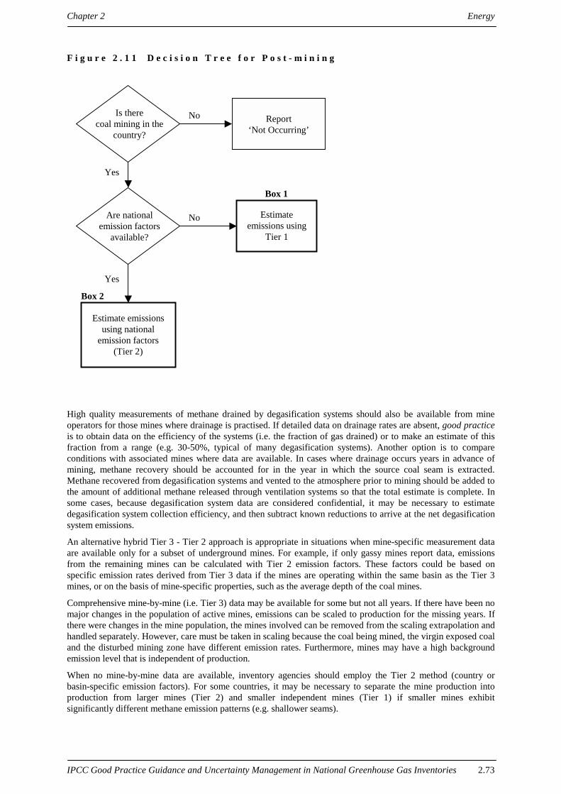
Chapter 2 Energy
IPCC Good Practice Guidance and Uncertainty Management in National Greenhouse Gas Inventories 2.73
F i g u r e 2 . 1 1 D e c i s i o n T r e e f o r P o s t - m i n i n g
High quality measurements of methane drained by degasification systems should also be available from mineoperators for those mines where drainage is practised. If detailed data on drainage rates are absent, good practiceis to obtain data on the efficiency of the systems (i.e. the fraction of gas drained) or to make an estimate of thisfraction from a range (e.g. 30-50%, typical of many degasification systems). Another option is to compareconditions with associated mines where data are available. In cases where drainage occurs years in advance ofmining, methane recovery should be accounted for in the year in which the source coal seam is extracted.Methane recovered from degasification systems and vented to the atmosphere prior to mining should be added tothe amount of additional methane released through ventilation systems so that the total estimate is complete. Insome cases, because degasification system data are considered confidential, it may be necessary to estimatedegasification system collection efficiency, and then subtract known reductions to arrive at the net degasificationsystem emissions.
An alternative hybrid Tier 3 - Tier 2 approach is appropriate in situations when mine-specific measurement dataare available only for a subset of underground mines. For example, if only gassy mines report data, emissionsfrom the remaining mines can be calculated with Tier 2 emission factors. These factors could be based onspecific emission rates derived from Tier 3 data if the mines are operating within the same basin as the Tier 3mines, or on the basis of mine-specific properties, such as the average depth of the coal mines.
Comprehensive mine-by-mine (i.e. Tier 3) data may be available for some but not all years. If there have been nomajor changes in the population of active mines, emissions can be scaled to production for the missing years. Ifthere were changes in the mine population, the mines involved can be removed from the scaling extrapolation andhandled separately. However, care must be taken in scaling because the coal being mined, the virgin exposed coaland the disturbed mining zone have different emission rates. Furthermore, mines may have a high backgroundemission level that is independent of production.
When no mine-by-mine data are available, inventory agencies should employ the Tier 2 method (country orbasin-specific emission factors). For some countries, it may be necessary to separate the mine production intoproduction from larger mines (Tier 2) and smaller independent mines (Tier 1) if smaller mines exhibitsignificantly different methane emission patterns (e.g. shallower seams).
Report‘Not Occurring’
Yes
Is therecoal mining in the
country?
Are nationalemission factors
available?
Box 1
No Estimateemissions using
Tier 1
Yes
No
Box 2
Estimate emissionsusing national
emission factors(Tier 2)

Energy Chapter 2
2.74 IPCC Good Practice Guidance and Uncertainty Management in National Greenhouse Gas Inventories
SURFACE MININGIt is not feasible to collect mine-by-mine Tier 3 measurement data for surface mines. The alternative is to collectdata on surface mine production and apply emission factors. For countries with significant coal production andmultiple coal basins, disaggregation to the basin level will improve accuracy. Given the uncertainty ofproduction-based emission factors, picking emission factors from the range specified by the IPCC Guidelines canprovide a reasonable estimate.
POST-MININGMethane still present in the coal after mining will escape to the atmosphere eventually. Measurement of post-mining emissions is not feasible, however, so an emission factor approach must be used. The Tier 2 and Tier 1methods in the IPCC Guidelines should be reasonable for this source, given the difficulty of obtaining betterdata.
RECOVERY OF METHANE FOR UTILISATION OR FLARINGIf methane is drained from coal seams and subsequently flared or used as a fuel, it is good practice to subtractthis amount from the total estimate of emissions. (Emissions from combustion of recovered methane should beaccounted for appropriately in the combustion section.) Where utilisation data are not directly available frommine operators, gas sales could be used as a proxy. If gas sales are unavailable, the alternative is to estimate theamount of utilised methane from the known efficiency specifications of the drainage system.
In some countries, it is common practice to drain and utilise coal bed methane many years prior to mining. Inother instances, gas wells are drilled in coal seams that are too deep to be mined. Fugitive emissions up to thepoint of utilisation should be counted in coal mining activities. Subsequent downstream emissions should beallocated to the source category appropriate to the manner of utilisation. Examples include oil and natural gaswhen the methane is fed to the natural gas grid and to electricity autoproducers when used to generate electricity.Note that where coal seam methane is recovered with no intention of mining the coal, emissions fall within the oiland natural gas source category.
The estimate of CH4 emissions from coal mining may or may not need to be corrected for the amount of gasreleased depending on whether:
• The coal is extracted a few years later and the CH4 emissions estimate for that year is based on averageemission factors that do not take account of early gas draining; in this case a correction is needed for the yearof extraction;
• The coal is extracted a few years later and the CH4 emissions estimate is based on direct emissionsmeasurements. In this case no correction is needed;
• The coal is never extracted (e.g. due to changes in plans or because it was never the intention). In this caseno correction is needed.
Flaring is an option for reducing methane emissions from coal mines, and is practised at some coal mines. Dataon the amount of methane flared should be obtained from mine operators with the same frequency ofmeasurement as pertains to underground mine emissions generally.
2.6.1.2 CHOICE OF EMISSION FACTORS
UNDERGROUND MININGTier 3: The Tier 3 method does not use production-based emission factors, but rather actual measurement datathat account for the temporal and spatial variability in coal mine emissions. As this is by far the most reliablemethod, inventory agencies should make every effort to collect these data if underground mining is a key sub-source category.
Tier 2: Country-specific emission factors can be obtained from sample ventilation air data, or from a quantitativerelationship that accounts for the gas content of the coal seam and the surrounding strata affected by the miningprocess. For a typical longwall operation, the amount of gas released comes from the coal being extracted andfrom the coal and any other gas bearing strata 150 m above and 50 m below the mined seam. Where suchrelationships are used, they should be peer-reviewed and well documented.
Tier 1: Inventory agencies choosing from the emission factor range (10-25 m3/tonne) in the Tier 1 methodologyshould consider country-specific variables such as depth of major coal seams. As gas content of coal usually

Chapter 2 Energy
IPCC Good Practice Guidance and Uncertainty Management in National Greenhouse Gas Inventories 2.75
increases with depth, the low end of the range should be chosen for average mining depths of <200 m, and fordepths of > 400 m the high value is appropriate. For intermediate depths, intermediate values can be chosen.
SURFACE MININGThere are few measurements of methane emissions from surface mining. They are difficult and expensive to carryout and no routine methods are currently available. Data on in-situ gas contents before overburden removal arealso very scarce, and in freshly uncovered coal the gas content is often close to zero. Where local data onemissions are available, they should be used.
For the Tier 1 approach, it is good practice to use the low end of the specific emission range for those mines withaverage overburden depths of <25 m and the high end for overburden depths over 50 meters. For intermediatedepths, intermediate values for the emission factors may be used. In the absence of data on overburden thickness,it is good practice to use an emission factor towards the high end of the range, namely 1.5 m3/tonne.
POST-MINING EMISSIONS – UNDERGROUNDMeasurements on coal as it emerges on a conveyor from a mine without pre-mining degasification indicate that25-40% of the in-situ gas is still in the coal (Williams and Saghafi, 1993). For mines that practice pre-drainage,the amount of gas in coal will be less by some unknown amount.
For mines with no pre-drainage, but with knowledge of the in-situ gas content, it is reasonable to set the postmining emission factor at 30% of this value. For mines with pre-drainage, an emission factor of 10% of the in-situ gas content is suggested. Where there are no in-situ gas content data or where pre-drainage is practised, butto an unknown extent, a reasonable approach is to increase overall underground emissions by 3% (Williams etal., 1993; Riemer, 1999).
POST-MINING EMISSIONS – SURFACE MININGUnless there are data to the contrary, emissions from this sub-source category are assumed to be negligible, as thegas content of surface coal are typically very low. Emissions can be viewed as being accommodated within thesurface emission factor.
2.6.1.3 CHOICE OF ACTIVITY DATA
For the Tier 3 method, coal production data are not necessary because actual measurements are available.However, it is good practice to collect and report these data to illustrate the relationship, if any, betweenunderground coal production and actual emissions on an annual basis.
The activity data for Tiers 1 and 2 are coal production. Mine operators are likely to know more about coalproduction than methane emissions, but inventory agencies need to consider how the information is collected. Forexample, using cleaned coal production data instead of raw coal production data will change the final emissionsestimate because emission factors are expressed in cubic meters per ton. Variable moisture content is anotherimportant issue.
If the data on raw coal production are available these should be used. If coal is not sent to a coal preparationplant or washery (used to upgrade the raw ‘run of mine’ coal by removing some of the mineral matter), then rawcoal production equals the amount of saleable coal.
Where coal is upgraded, some coal is rejected in the form of coarse discards containing high mineral matter andalso in the form of unrecoverable fines. The amount of waste is typically around 20% of the weight of raw coalfeed, but may vary considerably by country. Where activity data are in the form of saleable coal, some effortshould be made to determine the amount of production that is washed. Raw coal production is then estimated byincreasing the amount of ‘saleable coal’ by the fraction lost through washing.
An alternative approach that may be more suitable for mines whose raw coal output contains rock from the roofor floor as a deliberate part of the extraction process, is to use saleable coal data, provided the emission factorsused refer to clean coal not raw coal. This should be noted in the inventory.

Energy Chapter 2
2.76 IPCC Good Practice Guidance and Uncertainty Management in National Greenhouse Gas Inventories
2.6.1.4 COMPLETENESS
UNDERGROUND MININGThe estimate of emissions from underground mining should include both ventilation systems and degasificationsystems when both are present.
ABANDONED MINESNo method currently exists for estimating emissions from this sub-source category. For mines that are flooded,emissions are likely to be prevented, but some leakage is likely in mines that are sealed mechanically. Goodpractice is to record the date of mine closure and the method of sealing. Data on the size and depth of such mineswould be useful for any post hoc estimation.
CO2 IN SEAM GASCountries with significant quantities of CO2 in their coal seam gas should make efforts to evaluate or quantifythese emissions.
COAL FIRES, COMBUSTION AND OXIDATION OF WASTE COAL ANDOTHER CARBONACEOUS MATERIALS (CO2)IPCC recognises that there are emissions from these sub-source categories, but does not provide methods.Emissions could be significant, but are very difficult to estimate.
2.6.1.5 DEVELOPING A CONSISTENT TIME SERIES
In cases where an inventory agency moves from a Tier 1 or Tier 2 to a Tier 3 method, it may be necessary tocalculate implied emissions factors for years with measurement data, and apply these emission factors to coalproduction for years in which these data do not exist. It is important to consider if the composition of the minepopulation has changed dramatically during the interim period, because this could introduce uncertainty. Formines that have been abandoned since 1990, data may not be archived if the company disappears. These minesshould be treated separately when adjusting the time series for consistency. For good practice guidance onensuring time series consistency, see Chapter 7, Methodological Choice and Recalculation.
2.6.1.6 UNCERTAINTY ASSESSMENT
EMISSIONS
Tier 3Methane emissions from underground mines have a significant natural variability. Spot measurements of [CH4](the square brackets denote concentration) in ventilation air are probably accurate to ±20% depending on theequipment used. Time series data or repeat measurements will significantly reduce the uncertainty of annualemissions to ±5% for continuous monitoring, and 10-15% for every two weeks.22 Ventilation airflows are usuallyfairly accurately known (±2%).
Spot measurement of [CH4] in drained gas (degasification systems) is likely to be accurate to ±2% because of itshigher concentration. Measurements should be made with a frequency comparable to those for ventilation air toget representative sampling. Degasification flows are probably known to ±5%. Degasification flows based on gassales are also likely to have an uncertainty of at least ±5% due to the tolerances in pipeline gas quality.
As the gas liberated (gas make) by longwall mining can vary by a factor of two during the life of a longwall panel(a 1-2 km long x 200 m wide block of coal that is extracted in the course of 6-9 months by a single longwallmachine), it is necessary to make frequent measurements of underground mine emissions. Frequentmeasurements will also reduce the intrinsic errors in the measurement techniques. Mines with multiple longwall
22 The uncertainty ranges cited in this section represent an informal polling of assembled experts aiming to approximate the95% confidence interval around the central estimate.

Chapter 2 Energy
IPCC Good Practice Guidance and Uncertainty Management in National Greenhouse Gas Inventories 2.77
machines will be less subject to such wide fluctuations. There may also be uncertainty concerning utilisation ofany methane gas drained years before the source coal seam is extracted.
For a single longwall operation, with continuous or daily emission measurements, the accuracy of monthly orannual average emissions data is probably ±5%. The accuracy of spot measurements performed every two weeksis ±10%, at 3-monthly intervals ±30%. Aggregating emissions from mines based on the less frequent type ofmeasurement procedures will reduce the uncertainty caused by fluctuations in gas make. However, as fugitiveemissions are often dominated by contributions from only a small number of mines, it is difficult to estimate theextent of this improvement.
Tiers 1 and 2If a Tier 2 emission factor for underground mining is derived from Tier 3 data, then the errors or uncertainty inthe Tier 3 data can flow through to the derived emission factor for Tier 2. The following table gives someimpression of likely uncertainties:
TABLE 2.14
LIKELY UNCERTAINTIES OF COAL MINE METHANE EMISSION FACTORS
Method Underground Surface Post-Mining
Tier 2 ±50-75% factor of 2 ±50%
Tier 1 factor of 2 factor of 3 factor of 3
Source: Judgement by Expert Group (see Co-chairs, Editors and Experts; Fugitive Emissions from Coal Mining and Handling).
ACTIVITY DATACoal production: Tonnages are likely to be known to 1-2%, but if raw coal data are not available, then theuncertainty will increase to about ±5%, when converting from saleable coal production data. The data are alsoinfluenced by moisture content, which is usually present at levels between 5-10%, and may not be determinedwith great accuracy.
Apart from measurement uncertainty, there can be further uncertainties introduced by the nature of the statisticaldatabases that are not considered here. In countries with a mix of regulated and unregulated mines, activity datamay have an uncertainty of ±10%.
2 . 6 . 2 R e p o r t i n g a n d d o c u me n t a t i o nIt is good practice to document and archive all information required to produce the national emissions inventoryestimates as outlined in Section 8.10.1 of Chapter 8, Quality Assurance and Quality Control.
It is not practical to include all documentation in the national inventory report. However, the inventory shouldinclude summaries of methods used and references to source data such that the reported emissions estimates aretransparent and steps in their calculation may be retraced.
To ensure transparency, the following information should be supplied:
• Emissions by underground, surface, and post-mining components of CH4 and CO2 (where appropriate), themethod used for each of the sub-source categories, the number of active mines in each sub-source categoryand the reasons for the chosen EFs (e.g. depth of mining, data on in-situ gas contents etc.). The amount ofdrained gas and the degree of any mitigation or utilisation should be presented with a description of thetechnology used, where appropriate.
• Activity data: Specify the amount and type of production, underground and surface coal, listing raw andsaleable amounts where available.
• Where issues of confidentiality arise, the name of the mine need not be disclosed. Most countries will havemore than three mines, so mine-specific production cannot be back calculated from the emission estimates.

Energy Chapter 2
2.78 IPCC Good Practice Guidance and Uncertainty Management in National Greenhouse Gas Inventories
2 . 6 . 3 I n v e n t o r y q u a l i t y a s s u r a n c e / q u a l i t y c o n t r o l( Q A / Q C )
It is good practice to conduct quality control checks as outlined in Chapter 8, Quality Assurance and QualityControl, Table 8.1, Tier 1 General Inventory Level QC Procedures, and expert review of the emission estimates.Additional quality control checks as outlined in Tier 2 procedures in Chapter 8 and quality assurance proceduresmay also be applicable, particularly if higher tier methods are used to determine emissions from this sourcecategory. Inventory agencies are encouraged to use higher tier QA/QC for key source categories as identified inChapter 7, Methodological Choice and Recalculation.
In addition to the guidance in Chapter 8, specific procedures of relevance to this source category are outlinedbelow.
Comparison of emissions using alternative approachesThe inventory agency should compare the emission estimates for fugitive methane emissions from coal miningand handling using both Tier 1 and Tier 2 approaches. If direct measurements are available, these should also becompared to the Tier 1 and 2 estimates. Large discrepancies between the emission estimates should beinvestigated and explained. The results of such comparisons should be recorded for internal documentation.
Review of direct emission measurementsIf direct measurements are used to develop country-specific emission factors, it should be established whethermeasurements at the sites were made according to internationally recognised, standard methods. If themeasurement practices fail this criterion, then the use of these emissions data should be carefully evaluated,uncertainty estimates reconsidered, and qualifications documented. Frequent measurements are usually requiredby regulatory bodies. In the absence of such regulations, measurements should be done frequently enough(weekly if possible), as emissions rates may vary considerably over the year.
Emission factors checkThe inventory agency should compare measurement-based factors to IPCC defaults and factors developed byother countries with similar coal mining and handling characteristics. The QA/QC review associated with theoriginal data should be directly referenced in the documentation.
If IPCC default factors are used, the inventory agency should ensure that they are applicable and relevant to thecategory. If possible, the IPCC default factors should be compared to national or local data to provide furtherindication that the factors are applicable.
Activity data checkThe inventory agency should ensure that the data reflects raw coal production. Where possible, the data shouldbe compared to historical activity data to look for anomalies. Compare activity data between multiple references(e.g. national statistics and mill-level data). To check methane utilisation consistency, gas or electricity salescould be used as a cross-check.
External reviewThe inventory agency should arrange for an independent, objective review of calculations, assumptions, and/ordocumentation of the emissions inventory to be performed to assess the effectiveness of the QC programme. Thepeer review should be performed by expert(s) who are familiar with the source category and who understandinventory requirements.

Chapter 2 Energy
IPCC Good Practice Guidance and Uncertainty Management in National Greenhouse Gas Inventories 2.79
2 . 7 F U G I T I V E E M I S S I O N S F R O M O I L A N DG A S O P E R A T I O N S
2 . 7 . 1 M e t h o d o l o g i c a l i s s u e sFugitive emissions from oil and natural gas activities include all emissions from the exploration, production,processing, transport, and use of oil and natural gas, and from non-productive combustion (e.g. flaring and waste-gas incineration). It excludes use of oil and gas or derived products to provide energy for internal use, in energyproduction, processing and transport. The latter are considered fuel consumption and are addressed separately inthe IPCC Guidelines (Sections 1.3 to 1.5).
Fugitive emissions of methane (CH4), carbon dioxide (CO2) and nitrous oxide (N2O) from oil and gas operationsare a source of direct and indirect greenhouse gas emissions in many countries. Unfortunately, these emissionsare difficult to quantify accurately. This is largely due to the diversity of the industry, the large number andvariety of potential emission sources, the wide variations in emission-control levels, and the limited availabilityof emission-source data. The main emission assessment issues are:
• The use of simple production-based emission factors introduces excessive error;
• The application of rigorous bottom-up approaches requires expert knowledge and detailed data that may bedifficult and costly to obtain;
• Measurement programmes are time consuming and very costly to perform.
If a rigorous bottom-up approach is chosen, then it is good practice to involve technical representatives from theindustry in the development of the inventory.
2.7.1.1 CHOICE OF METHOD
The IPCC Guidelines describe two methods to calculate CH4 emissions from both the oil and gas industries(called Tier 1 and Tier 3), and one additional method (called Tier 2) to calculate CH4 emissions only from oilsystems. The Tier 3 method is a rigorous source-specific evaluation, requiring detailed inventories ofinfrastructure, and detailed bottom-up emission factors. The Tier 2 approach for CH4 emissions from the oilindustry is based on a mass balance estimate of the maximum amount of CH4 that could be emitted. The Tier 1method uses aggregate production-based emission factors and national production data.23
Good practice is to disaggregate the industry into the applicable segments and subcategories indicated inTable 2.15, Major Categories and Subcategories in the Oil and Gas Industry, and then evaluate the emissionsseparately for each of these parts. The approach to estimate emissions from each segment should becommensurate with the emissions level and the available resources. Consequently, it may be appropriate to applydifferent approaches to different parts of the industry, and possibly even include some direct monitoring ofemission sources. The overall approach, over time, should be one of progressive refinement to address the areasof greatest uncertainty and consequence, and to capture the impact of specific control measures.
Figure 2.12 provides a general decision tree for Natural Gas Systems for selecting an appropriate approach for agiven segment of the natural gas system. Similarly, Figures 2.13 and 2.14 apply to oil production and transportsystems, and to oil upgraders and refineries, respectively.
23 There is no Tier 2 method for natural gas systems in the IPCC Guidelines.

Energy Chapter 2
2.80 IPCC Good Practice Guidance and Uncertainty Management in National Greenhouse Gas Inventories
F i g u r e 2 . 1 2 D e c i s i o n T r e e f o r N a t u r a l G a s S y s t e m s
Box 2 Box 3
Box 1
Yes
Report‘Not Occurring’
Is therea natural gas system
in the country?
Box 4
Estimate emissionsusing rigorous emissionsource models (Tier 3)
Yes
No
Are actualmeasurements or
sufficient data available toestimate emissions using
rigorous emissionsource models?
Are detailedinfrastructure data
available?
Are nationalemission factors
available?
IfFugitive
Emissions from Oil andGas Operations are key source
categories, are Natural GasSystems significant?
(Note 1)
Estimate emissionsusing a Tier 1
approach
Collect detailedinfrastructure
data
Estimate emissions usingappropriate emission
factors from the generalliterature and
infrastructure data
Estimate emissionsusing national emission
factors andinfrastructure data
Yes
Yes
Yes
NoNo
No
No
Note 1: A key source category is one that is prioritised within the national inventory system because its estimate has a significantinfluence on a country’s total inventory of direct greenhouse gases in terms of the absolute level of emissions, the trend in emissions, orboth. (See Chapter 7, Methodological Choice and Recalculation, Section 7.2, Determining National Key Source Categories.)

Chapter 2 Energy
IPCC Good Practice Guidance and Uncertainty Management in National Greenhouse Gas Inventories 2.81
F i g u r e 2 . 1 3 D e c i s i o n T r e e f o r C r u d e O i l P r o d u c t i o n a n d T r a n s p o r t
Yes
Report‘Not Occurring’
Is therecoal mining in the
country?
Yes
No
Is itpossible to collect
or estimate data for thevented, flared, utilised conserved
and reinjected volumes ofassociated and solution
gas production?
Is itpossible to estimate
total associated and solutiongas volumes (e.g. based on GOR
data (Note 2)), and is morethan 20% vented
or flared?
If FugitiveEmissions from Oil
and Gas Operations are keysource Categories, is thesub-source significant?
(Note 1)
Are detailedinfrastructure data
available?
Collect orestimate detailed
infrastructure data
Are nationalemission factors
available?
Box 4Estimate emissionsusing appropriate
emission factors fromthe general literature
Box 3
Estimate emissionsusing a Tier 3approach and
national emissionfactors
Box 2
Estimate emissionsusing a Tier 2
approach
Box 1
Estimate emissionsusing a Tier 1
approach
Yes
No
No
No
Collect data on associatedand solution gas
Yes
No No
YesYes
Note 1: A key source category is one that is prioritised within the national inventory system because its estimate has a significantinfluence on a country’s total inventory of direct greenhouse gases in terms of the absolute level of emissions, the trend in emissions, orboth. (See Chapter 7, Methodological Choice and Recalculation, Section 7.2, Determining National Key Source Categories.)
Note 2: GOR stands for Gas/Oil Ratio.

Energy Chapter 2
2.82 IPCC Good Practice Guidance and Uncertainty Management in National Greenhouse Gas Inventories
F i g u r e 2 . 1 4 D e c i s i o n T r e e f o r C r u d e O i l R e f i n i n g a n d U p g r a d i n g
Box 2
Report‘Not Occurring’
Yes
No
Is therecrude oil refining
or upgrading in thecountry?
Is itpossible to estimateflared and vented
volumes?
If FugitiveEmissions from Oil
and Gas Operations are keysource categories, is the sub-
source significant?(Note 1)
Estimate emissionsusing a Tier 3
approach
Collect data onventing and
flaring
Box 1
Yes
No Estimateemissions using aTier 1 approach
Yes
No
Note 1: A key source category is one that is prioritised within the national inventory system because its estimate has a significantinfluence on a country’s total inventory of direct greenhouse gases in terms of the absolute level of emissions, the trend in emissions, orboth. (See Chapter 7, Methodological Choice and Recalculation, Section 7.2, Determining National Key Source Categories.)

Chapter 2 Energy
IPCC Good Practice Guidance and Uncertainty Management in National Greenhouse Gas Inventories 2.83
TABLE 2.15
MAJOR CATEGORIES AND SUBCATEGORIES IN THE OIL AND GAS INDUSTRY
Industry Segment Sub-Categories
Wells Drilling
Testing
Servicing
Gas Production Dry Gasa
Sweet Gasb
Sour Gasc
Gas Processing Sweet Gas Plants
Sour Gas Plants
Deep-cut Extraction Plants
Gas Transmission & Storage Pipeline Systems
Storage Facilities
Gas Distribution Rural Distribution
Urban Distribution
Liquefied Gases Transport Condensate
Liquefied Petroleum Gas (LPG)
Liquefied Natural Gas (LNG) (including associatedliquefaction and gasification facilities)
Oil Production Conventional Oil
Heavy Oil (Primary Production)
Heavy Oil (Enhanced Production)
Crude Bitumen
Synthetic Crude Oil (From Oilsands)
Synthetic Crude Oil (From Oil Shales)
Oil Upgrading Crude Bitumen
Heavy Oil
Waste Oil Reclaiming None
Oil Transport Marine
Pipelines
Tanker Trucks and Rail Cars
Oil Refining Heavy Oil
Conventional and Synthetic Crude Oila Dry gas is natural gas that does not require any hydrocarbon dew-point control to meet sales gas specifications. However, it may stillrequire treating to meet sales specifications for water and acid gas (i.e. H2S and CO2) content. Dry gas is usually produced from shallow(less than 1000 m deep) gas wells.b Sweet gas is natural gas that does not contain any appreciable amount of H2S (i.e. does not require any treatment to meet sales gasrequirements for H2S).c Sour gas is natural gas that must be treated to satisfy sales gas restrictions on H2S content.

Energy Chapter 2
2.84 IPCC Good Practice Guidance and Uncertainty Management in National Greenhouse Gas Inventories
It is good practice to use the Tier 3 approach which will produce the most accurate emissions estimate. However,the ability to use a Tier 3 approach will depend on the availability of detailed production statistics andinfrastructure data, and it may not be possible to apply it under all circumstances. A Tier 2 (mass balance)approach is primarily intended for application to oil systems where the majority of the associated and solutiongas production is vented or flared. While much less reliable when applied to oil systems with gas conservation orto gas systems, a crude mass balance approach based on national production statistics may sometimes offer agreater degree of confidence than that offered by the Tier 1 approach. In such cases, the net balancing term (i.e.unaccounted-for losses) may be comparable to total fugitive emissions from non-venting or flaring sources. TheTier 1 approach is susceptible to substantial uncertainties and may easily be in error by an order-of-magnitude ormore. For this reason, it should only be used as a last resort option.
2.7.1.2 CHOICE OF EMISSION FACTORS
Emission factors for conducting Tier 2 and Tier 3 assessments are not provided in the IPCC Guidelines due tothe large amount of such information. Moreover, these data are continually being updated to include additionalmeasurement results and to reflect development and penetration of new control technologies and requirements.Regular reviews of the literature should be conducted to ensure that the best available factors are being used, andthe references for the chosen values should be clearly documented. Typically, emission factors are developed andpublished by environmental agencies and industry associations, and it will be necessary to develop inventoryestimates in consultation with these organisations.
The selected emission factors must be valid for the given application and be expressed on the same basis as theactivity data. It also may be necessary to apply other types of factors to correct for site and regional differences inoperating conditions and design and maintenance practices, for example:
• Composition profiles of gases from particular oil and gas fields to correct for the amount of CH4, raw CO2and other target pollutants in the emissions;
• Annual operating hours to correct for the amount of time a source is in active service;
• Efficiencies of the specific control measures used.
The following are additional matters to consider in choosing emission factors:
• It is important to assess the applicability of the selected factors for the target application to ensuresimilar/comparable source behaviour and characteristics;
• In the absence of better data, it may sometimes be necessary to apply factors reported for other regions thatpractice similar levels of emission control and feature comparable types of equipment;
• Where measurements are performed to develop new emission factors, only recognised or defensible testprocedures should be applied. The method and quality assurance (QA)/quality control (QC) proceduresshould be documented, the sampled sources should be representative of typical variations in the overallsource population, and a statistical analysis should be conducted to establish the 95% confidence interval onthe average results.
New Tier 1 emission factors are presented in Table 2.16, Refined Tier 1 Emission Factors based on NorthAmerican Data. Although still a simplified means of estimating fugitive emissions, the new factors allow forimproved correlation of emissions with commonly-available activity data, and may be expected to limituncertainties to within an order of magnitude. The improved correlations are achieved through increaseddisaggregation of the industry and, in several cases, by switching to different activity parameters. For example,fugitive emissions from gas transmission and distribution systems do not correlate well with throughput, and arebetter related to lengths of pipeline.
The new factors are derived from detailed emission inventory results for Canada and the United States, and arepresented as examples. Notwithstanding this, these values may be applied to regions outside of North Americathat practice similar levels of emissions control and feature comparable types and quality of equipment. Evenwhere moderate regional differences exist, the new factors may still offer more reliable results than that obtainedfrom use of the factors given in the IPCC Guidelines. Nonetheless, it is good practice to consider the impact ofregional differences before adopting a specific set of factors. In the absence of data for a particular industrysegment or where conditions in the United States and Canada are not representative, the emission factors given inthe IPCC Guidelines, Reference Manual Tables 1-57, Summary of Methane Emission Factors, and Table 1-58,Revised Regional Emission Factors for Methane from Oil and Gas Activities should be used.

Chapter 2 Energy
IPCC Good Practice Guidance and Uncertainty Management in National Greenhouse Gas Inventories 2.85
In general, the developed factors reflect the following practices and state of the oil and gas industry:
• Most associated gas is conserved;
• Sweet waste gas is vented;
• Sour waste gas is flared;
• Many gas transmission companies are voluntarily implementing programmes to reduce methane losses due tofugitive equipment leaks;
• The oil and gas industry is mature and actually in decline in many areas;
• System reliability is high;
• Equipment is generally well maintained and high-quality components are used;
• Line breaks and well blowouts are rare;
• The industry is highly regulated and these regulations are generally well enforced.

Energy Chapter 2
2.86 IPCC Good Practice Guidance and Uncertainty Management in National Greenhouse Gas Inventories
TABLE 2.16
REFINED TIER 1 EMISSION FACTORS FOR FUGITIVE EMISSIONS FROM OIL AND GAS OPERATIONSBASED ON NORTH AMERICAN DATA
Default emission factora,bCategory Sub-Category
EmissionType
CH4 CO2 N2O
Units of Measure
Drilling Allc 4.3E-07 2.8E-08 0 Gg per number of wells drilled
Testing All 2.7E-04 5.7E-03 6.8E-08 Gg per number of wells drilled
Wells
Servicing All 6.4E-05 4.8E-07 0 Gg/yr per number of producingand capable wells
Fugitivesd 2.6E-03 to2.9E-03
9.5E-05 0 Gg per 106 m3 gas productionGasProduction
All
Flaringe 1.1E-05 1.8E-03 2.1E-08 Gg per 106 m3 gas production
Fugitives 6.9E-04 to10.7E-04
2.7E-05 0 Gg per 106 m3 gas receiptsSweet GasPlants
Flaring 1.3E-05 2.1E-03 2.5E-08 Gg per 106 m3 gas receipts
Fugitives 2.1E-04 2.9E-05 0 Gg per 106 m3 gas receipts
Flaring 2.9E-05 4.6E-03 5.4E-08 Gg per 106 m3 gas receipts
Sour GasPlants
Raw CO2Venting
0 7.1E-02 0 Gg per 106 m3 gas receipts
Fugitives 1.0E-05 3.0E-07 0 Gg per 106 m3 gas receipts
GasProcessing
Deep-cutExtractionPlants Flaring 6.2E-06 9.7E-04 1.2E-08 Gg per 106 m3 gas receipts
Fugitivesf 2.1E-03 to2.9E-03
1.6E-05 0 Gg per year and per km oftransmission pipeline
Transmission
Ventingg 0.8E-03 to1.2E-03
8.5E-06 0 Gg per year and per km oftransmission pipeline
GasTransmission& Storage
Storage All 4.3E-04 to42.0E-04
0 0 Gg per year and per 106 m3 gaswithdrawals
GasDistribution
All All 5.2E-04 to7.1E-04
0 0 Gg per year and per km ofdistribution mains
Condensate All 1.1E-04 7.2E-06 0 Gg per 103 m3 Condensate andPentanes Plus
Natural GasLiquidsTransport
LiquefiedPetroleumGas
All 0 4.3E-04 2.2E-09 Gg per 103 m3 LPG
Fugitives 1.4E-03 to1.5E-03
2.7E-04 0 Gg per 103 m3 conventional oilproduction
Venting 6.2E-05 to270E-05
1.2E-05 0 Gg per 103 m3 conventional oilproduction
ConventionalOil
Flaring 0.5E-05 to27E-05
6.7E-02 6.4E-07 Gg per 103 m3 conventional oilproduction
Fugitives 0.8E-04 to12E-04
6.7E-06 0 Gg per 103 m3 heavy oilproduction
Venting 2.1E-02 to2.7E-02
5.0E-05 0 Gg per 103 m3 heavy oilproduction
OilProduction
Heavy Oil
Flaring 0.5E-04 to2.0E-04
4.9E-02 4.6E-07 Gg per 103 m3 heavy oilproduction

Chapter 2 Energy
IPCC Good Practice Guidance and Uncertainty Management in National Greenhouse Gas Inventories 2.87
TABLE 2.16 (CONTINUED)
REFINED TIER 1 EMISSION FACTORS FOR FUGITIVE EMISSIONS FROM OIL AND GAS OPERATIONSBASED ON NORTH AMERICAN DATA
Default emission factora,bCategory Sub-Category
EmissionType
CH4 CO2 N2O
Units of Measure
Fugitives 1.0E-04 1.2E-04 0 Gg per 103 m3 crude bitumenproduction
Venting 1.0E-03 1.2E-03 0 Gg per 103 m3 crude bitumenproduction
CrudeBitumen
Flaring 8.8E-05 2.2E-02 2.4E-07 Gg per 103 m3 crude bitumenproduction
SyntheticCrude (fromOilsands)
All 2.3E-03 0 0 Gg per 103 m3 synthetic crudeproduction from oilsands
OilProduction(continued)
SyntheticCrude (fromOil Shale)
All NA NA NA Gg per 103 m3 synthetic crudeproduction from oil shale
OilUpgrading
All All ND ND ND Gg per 103 m3 oil upgraded
Pipelines All 5.4E-06 4.9E-07 0 Gg per 103 m3 oil transported bypipeline
TankerTrucks andRail Cars
Venting 2.5E-05 2.3E-06 0 Gg per 103 m3 oil transported byTanker Truck
Oil Transport
Loading ofOff-shoreProductionon TankerShips
Venting NAh NAh NAh Gg per 103 m3 oil transported byTanker Truck
NA - Not Applicable ND - Not Determineda While the presented emission factors may all vary appreciably between countries, the greatest differences are expected to occur withrespect to venting and flaring, particularly for oil production due to the potential for significant differences in the amount of gasconservation and utilisation practised.b The range in values for fugitive emissions is attributed primarily to differences in the amount of process infrastructure (e.g. averagenumber and sizes of facilities) per unit of gas throughput.c ‘All’ denotes all fugitive emissions as well as venting and flaring emissions.d ‘Fugitives’ denotes all fugitives emissions including those from fugitive equipment leaks, storage losses, use of natural gas as thesupply medium for gas-operated devices (e.g. instrument control loops, chemical injection pumps, compressor starters, etc.), and ventingof still-column off-gas from glycol dehydrators.e ‘Flaring’ denotes emissions from all continuous and emergency flare systems. The specific flaring rates may vary significantly betweencountries. Where actual flared volumes are known, these should be used to determine flaring emissions rather than applying thepresented emission factors to production rates. The emission factors for direct estimation of CH4, CO2 and N2O emissions from reportedflared volumes are 0.012, 2.0 and 0.000023 Gg, respectively, per 106 m3 of gas flared based on a flaring efficiency of 98% and a typicalgas analysis at a gas processing plant (i.e. 91.9% CH4, 0.58% CO2, 0.68% N2 and 6.84% non-methane hydrocarbons by volume).f The larger factor reflects the use of mostly reciprocating compressors on the system while the smaller factor reflects mostly centrifugalcompressors.g ‘Venting’ denotes reported venting of waste associated and solution gas at oil production facilities and waste gas volumes fromblowdown, purging and emergency relief events at gas facilities. Where actual vented volumes are known, these should be used todetermine venting emissions rather than applying the presented emission factors to production rates. The emission factors for directestimation of CH4 and CO2 emissions from reported vented volumes are 0.66 and 0.0049 Gg, respectively, per 106 m3 of gas ventedbased on a typical gas analysis for gas transmission and distribution systems (i.e. 97.3% CH4, 0.26% CO2, 1.7% N2 and 0.74% non-methane hydrocarbons by volume).h While no factors are available for marine loading of offshore production for North America, Norwegian data indicate a CH4 emissionfactor of 1.0 to 3.6 Gg/103 m3 of oil transferred (derived from data provided by Norwegian Pollution Control Authority, 2000).
Sources: Canadian Association of Petroleum Producers (1999); GRI/US EPA (1996); US EPA (1999).

Energy Chapter 2
2.88 IPCC Good Practice Guidance and Uncertainty Management in National Greenhouse Gas Inventories
2.7.1.3 CHOICE OF ACTIVITY DATA
The activity data required to estimate fugitive emissions from oil and gas activities may include productionstatistics, infrastructure data (e.g. inventories of facilities/installations, process units, pipelines, and equipmentcomponents), and reported emissions from spills, accidental releases, and third-party damages. The basic activitydata required for each tier and each type of primary source are summarised in Table 2.17, Typical Activity DataRequirements for each Assessment Approach by Type of Primary Source Category. Specific matters to considerin compiling this information include the following:
• Production statistics should be disaggregated to capture changes in throughputs (e.g. due to imports, exports,reprocessing, withdrawals, etc.) in progressing through oil and gas systems.
• Production statistics or disposition analyses24 may not agree between different reporting agencies eventhough they are based on the same original measurement results (e.g. due to possible differences interminology and potential errors in summarising these data). These discrepancies may be used as anindication of the uncertainty in the data. Additional uncertainty will exist if there is any inherent bias in theoriginal measurement results (for example, sales meters are often designed to err in favour of the customer,and liquid handling systems will have a negative bias due to evaporation losses). Random metering andaccounting errors may be assumed to be negligible when aggregated over the industry.
• Production statistics provided by national bureaux should be used in favour of those available frominternational bodies, such as the IEA or the UN, due to their generally better reliability and disaggregation.Regional, provincial/state and industry reporting groups may offer even more disaggregation.
• Reported vented and flared volumes may be highly suspect since these values are usually estimates and notbased on actual measurements. Additionally, the values are often aggregated and simply reported as flaredvolumes. Operating practices of each segment of the industry should be reviewed to determine if the reportedvolumes are actually vented or flared, or to develop appropriate apportioning of venting relative to flaring.Audits or reviews of each industry segment should also be conducted to determine if all vented/flaredvolumes are actually reported (for example, solution gas emissions from storage tanks and treaters,emergency flaring/venting, leakage into vent/flare systems, and blowdown and purging volumes may notnecessarily be accounted for).
• Infrastructure data are more difficult to obtain than production statistics. Information concerning thenumbers and types of major facilities and the types of processes used at these facilities may often beavailable from regulatory agencies and industry groups, or directly from the actual companies.
• Information on minor facilities (e.g. numbers of field dehydrators and field compressors) usually is notavailable, even from oil and gas companies. Consequently, assumptions must be made, based on local designpractices, to estimate the numbers of these facilities. This may require some fieldwork to developappropriate estimation factors or correlations.
• Many companies use computerised inspection-and-maintenance information management systems. Thesesystems can be a very reliable means of counting major equipment units (e.g. compressor units, processheaters and boilers, etc.) at selected facilities. Also, some departments within a company may maintaindatabases of certain types of equipment or facilities for their own specific needs (e.g. tax accounting,production accounting, insurance records, quality control programmes, safety auditing, license renewals,etc.). Efforts should be made to identify these potentially useful sources of information.
24 A disposition analysis provides a reconciled accounting of produced hydrocarbons from the wellhead, or point of receipt,through to the final sales point or point of export. Typical disposition categories include flared/vented volumes, fuel usage,system losses, volumes added to/removed from inventory/storage, imports, exports, etc.

Chapter 2 Energy
IPCC Good Practice Guidance and Uncertainty Management in National Greenhouse Gas Inventories 2.89
TABLE 2.17
TYPICAL ACTIVITY DATA REQUIREMENTS FOR EACH ASSESSMENT APPROACH FOR FUGITIVE EMISSIONS FROM OIL ANDGAS OPERATIONS BY TYPE OF PRIMARY SOURCE CATEGORY
Assessment Tier Primary Source Category Minimum Required Activity Data
1 All Oil and Gas Throughputs
2 Oil Systems Gas to Oil Ratios
Flared and Vented Volumes
Conserved Gas Volumes
Reinjected Gas Volumes
Utilised Gas Volumes
Gas Compositions
Process Venting/Flaring Reported Volumes
Gas Compositions
Proration Factors for Splitting Venting from Flaring
Storage Losses Solution Gas Factors
Liquid Throughputs
Tank Sizes
Vapour Compositions
Equipment Leaks Facility/Installation Counts by Type
Processes Used at Each Facility
Equipment Component Schedules by Type of Process Unit
Gas/Vapour Compositions
Gas-Operated Devices Schedule of Gas-operated Devices by Type of Process Unit
Gas Consumption Factors
Type of Supply Medium
Gas Composition
Accidental Releases & Third-Party Damages
Incident Reports/Summaries
Gas Migration to the Surface& Surface Casing Vent Blows
Average Emission Factors & Numbers of Wells
Drilling Number of Wells Drilled
Reported Vented/Flared Volumes from Drill Stem Tests
Typical Emissions from Mud Tanks
Well Servicing Tally of Servicing Events by Types
Pipeline Leaks Type of Piping Material
Length of Pipeline
3
Exposed Oilsands/Oil Shale Exposed Surface Area
Average Emission Factors
Component counts by type of process unit may vary dramatically between facilities and countries due todifferences in design and operating practices. Thus, while initially it may be appropriate to use values reported inthe general literature, countries should strive to develop their own values.
Use of consistent terminology and clear definitions is critical in developing counts of facilities and equipmentcomponents, and to allow any meaningful comparisons of the results with others.

Energy Chapter 2
2.90 IPCC Good Practice Guidance and Uncertainty Management in National Greenhouse Gas Inventories
Some production statistics may be reported in units of energy (based on their heating value) and will need to beconverted to a volume basis, or vice versa, for application of the available emission factors. Typically, whereproduction values are expressed in units of energy, it is in terms of the gross (or higher) heating value of theproduct. However, where emission factors are expressed on an energy basis it is normally in terms of the net (orlower) heating value of the product. To convert from energy data on a GCV basis to a NCV basis, theInternational Energy Agency assumes a difference of 5% for oil and 10% for natural gas. Individual natural gasstreams that are either very rich or high in impurities may differ from the average value given above. Emissionfactors and activity data must be consistent with each other.
In comparing fugitive emissions from the oil and gas industry in different countries it is important to consider theimpact of oil and gas imports and exports, as well as the types of oil and gas activities and the levels of emissioncontrol. Otherwise, emissions viewed on either a per-unit-consumption or a per-unit-production basis will bemisleading.
Production activities will tend to be the major contributor to fugitive emissions from oil and gas activities incountries with low import volumes relative to consumption and export volumes. Gas transmission anddistribution and petroleum refining will tend to be the major contributors to these emissions in countries withhigh relative import volumes. Overall, net importers will tend to have lower specific emissions than net exporters.
2.7.1.4 COMPLETENESS
Completeness is a significant issue in developing an inventory of fugitive emissions for the oil and gas industry.It can be addressed through direct comparisons with other countries and, for refined inventories, throughcomparisons between individual companies in the same industry segment and subcategory. This requires use ofconsistent definitions and classification schemes. In Canada, the upstream petroleum industry has adopted abenchmarking scheme that compares the emission inventory results of individual companies in terms ofproduction-energy intensity and production-carbon intensity. Such benchmarking allows companies to assesstheir relative environmental performance. It also flags, at a high level, anomalies or possible errors that should beinvestigated and resolved.
The indicative factors presented in Table 2.18 may be used to help assess completeness and to qualify specificmethane losses as being low, medium or high. Specific methane losses which are appreciably less than the lowbenchmark or greater than the high benchmark should be explained. The ranking of specific methane lossesrelative to the presented activity data should not be used as a basis for choosing the most appropriate assessmentapproach; rather, total emissions (i.e. the product of activity data and emission factors), the complexity of theindustry and available assessment resources should all be considered.

Chapter 2 Energy
IPCC Good Practice Guidance and Uncertainty Management in National Greenhouse Gas Inventories 2.91
TABLE 2.18
CLASSIFICATION OF GAS LOSSES AS LOW, MEDIUM OR HIGH AT SELECTED TYPES OF NATURAL GAS FACILITIES
Yearly emission factors
Facilities Activity dataLow Medium High Units of
Measure
Production andProcessing
Net gas production (i.e. marketedproduction)
0.05 0.2 0.7 % of netproduction
TransmissionPipeline Systems
Length of transmission pipelines 200 2 000 20 000 m3/km/yr
CompressorStations
Installed compressor capacity 6 000 20 000 100 000 m3/MW/yr
UndergroundStorage
Working capacity of undergroundstorage stations
0.05 0.1 0.7 % of workinggas capacity
LNG Plant(liquefaction orregasification)
Gas throughput 0.005 0.05 0.1 % of throughput
Meter andRegulator Stations
Number of stations 1 000 5 000 50 000 m3/station/yr
Distribution Length of distribution network 100 1 000 10 000 m3/km/yr
Gas Use Number of gas appliances 2 5 20 m3/appliance/yr
Source: Adapted from currently unpublished work by the International Gas Union, and based on data for a dozen countries includingRussia and Algeria.
Smaller individual sources, when aggregated nationally over the course of a year, may often be significant totalcontributors. Therefore, good practice is not to disregard them unless their collective contribution to totalfugitive emissions is proven to be negligible. Conversely, once a thorough assessment has been done, a basisexists for simplifying the approach and better allocating resources in the future to best reduce uncertainties in theresults.
2.7.1.5 DEVELOPING A CONSISTENT TIME SERIES
Ideally, emission estimates will be prepared for the base year and subsequent years using the same method.Where some historical data are missing it should still be possible to use source-specific measurements combinedwith backcasting techniques to establish an acceptable relationship between emissions and activity data in thebase year. Approaches for doing this will depend on the specific situation, and are discussed in general terms inChapter 7, Methodological Choice and Recalculation, Section 7.3.2.2, Alternative Recalculation Techniques.
While establishing base year emission levels is meaningful and important at a regional or national level, it isoften a misleading indicator at the company level due to frequent mergers, divestitures and acquisitions in manyareas. This may be an issue where national inventories are developed based on a rollup of company-levelinventories, and some extrapolations or interpolations are required.
Where changes in methods and emission factors are substantial, the whole time series should be recalculated andreported in a transparent manner.
2.7.1.6 UNCERTAINTY ASSESSMENT
Sources of error occur in the following areas:
• Measurement errors;
• Extrapolation errors;
• Inherent uncertainties of the selected estimation techniques;
• Missing or incomplete information regarding the source population and activity data;

Energy Chapter 2
2.92 IPCC Good Practice Guidance and Uncertainty Management in National Greenhouse Gas Inventories
• Poor understanding of temporal and seasonal variations in the sources;
• Over or under accounting due to confusion or inconsistencies in category divisions and source definitions;
• Misapplication of activity data or emission factors;
• Errors in reported activity data;
• Missed accounting of intermediate transfer operations and reprocessing activities (e.g. repeat dehydration ofgas streams [in the field, at the plant, and following storage], treating of slop and foreign oil receipts) due topoor or no documentation of such activities;
• Variances in the effectiveness of control devices and missed accounting of control measures;
• Data-entry and calculation errors.
Due to the complexity of the oil and gas industry, it is difficult to quantify the net uncertainties in the overallinventories, emission factors and activity data. While some semi-quantitative analyses have been conducted, amore thorough quantitative analysis is warranted.
High-quality refined emissions factors for most gases may be expected to have errors in the order of ±25percent.25 Factors based on stochiometric ratios may be much better (e.g. errors of ±10%). Gas compositions areusually accurate to within ±5% on individual components. Flow rates typically have errors of ±3% or less forsales volumes and ±15% or more for other volumes.
A high-quality bottom-up (Tier 3) inventory of fugitive methane losses from either oil or gas activities might beexpected to have errors of ±25 to ±50%. In comparison, default production-based emission factors for methanelosses may easily be in error by an order of magnitude or more. Inventories of fugitive CH4 and CO2 emissionsfrom venting and flaring activities will be quite reliable if the raw gaseous composition and actual vented andflared volumes are accurately known. Estimates of fugitive N2O emissions will be least reliable but will only be aminor contributor to total fugitive greenhouse gas emissions from oil and gas activities.
Estimates of emission reductions from individual control actions may be accurate to within a few percent to±25% depending on the number of subsystems or sources considered.
2 . 7 . 2 R e p o r t i n g a n d d o c u me n t a t i o nIt is good practice to document and archive all information required to produce the national emissions inventoryestimates as outlined in Section 8.10.1 of Chapter 8, Quality Assurance and Quality Control.
It is not practical to include all documentation in the national inventory report. However, the inventory shouldinclude summaries of methods used and references to source data such that the reported emissions estimates aretransparent and steps in their calculation may be retraced.
Some examples of specific documentation and reporting relevant to this source category are provided below.
Documentation is particularly important where a Tier 3 approach is used since the IPCC Guidelines do notdescribe a standard Tier 3 approach for the oil and gas sector. There is a wide range in what potentially may beclassified as a Tier 3 approach, and correspondingly, in the amount of uncertainty in the results.
If available, summary performance and activity indicators should be reported to help put the results inperspective (e.g. total production levels and transportation distances, net imports and exports, and specificenergy, carbon and emission intensities). Reported emission results should also include a trend analysis to showchanges in emissions and activity data over time. The expected accuracy of the results should be stated and theareas of greatest uncertainty clearly noted. This is critical for proper interpretation of the results and any claimsof net reductions.
The current trend by some government agencies and industry associations is to develop detailed methodologymanuals and reporting formats for specific segments and subcategories of the industry. This is perhaps the mostpractical means of maintaining, documenting and disseminating the subject information. However, all suchinitiatives must conform to the common framework established in the IPCC Guidelines so that the emissionresults can be compared across countries.
25 The percentages cited in this section represent an informal polling of assembled experts aiming to approximate the 95%confidence interval around the central estimate.

Chapter 2 Energy
IPCC Good Practice Guidance and Uncertainty Management in National Greenhouse Gas Inventories 2.93
Since emission factors and estimation procedures are continually being improved and refined, it is possible forchanges in reported emissions to occur without any real changes in actual emissions. Accordingly, the basis forany changes in results between inventory updates should be clearly discussed and those due strictly to changes inmethods and factors should be highlighted.
The issue of confidential business information will vary from region to region depending on the number of firmsin the market and the nature of the business. The significance of this issue tends to increase in progressingdownstream through the oil and gas industry. A common means to address such issues where they do arise is toaggregate the data using a reputable independent third party.
2 . 7 . 3 I n v e n t o r y q u a l i t y a s s u r a n c e / q u a l i t y c o n t r o l( Q A / Q C )
It is good practice to conduct quality control checks as outlined in Chapter 8, Quality Assurance and QualityControl, Table 8.1, Tier 1 General Inventory Level QC Procedures, and expert review of the emission estimates.Additional quality control checks as outlined in Tier 2 procedures in Chapter 8 and quality assurance proceduresmay also be applicable, particularly if higher tier methods are used to determine emissions from this sourcecategory. Inventory agencies are encouraged to use higher tier QA/QC for key source categories as identified inChapter 7, Methodological Choice and Recalculation.
In addition to the guidance in Chapter 8, specific procedures of relevance to this source category are outlinedbelow.
Emission inventories for large, complex oil and gas industries will be susceptible to significant errors due tomissed or unaccounted sources. To minimise such errors, it is important to obtain active industry involvement inthe preparation and refinement of these inventories.
Review of direct emission measurementsIf direct measurements are used to develop country-specific emission factors, the inventory agency shouldestablish whether measurements at the sites were made according to recognised standard methods. If themeasurement practices fail this criterion, then the use of these emissions data should be carefully evaluated,estimates reconsidered, and qualifications documented.
Emission factors checkThe inventory agency should compare measurement-based factors to IPCC default factors and factors developedby other countries with similar industry characteristics. If IPCC default factors are used, the inventory agencyshould ensure that they are applicable and relevant to the category. If possible, the IPCC default factors should becompared to national or local data to provide further indication that the factors are applicable.
Activity data checkSeveral different types of activity data may be required for this source category, depending on which method isused. The inventory agency should check different types of activity data against each other to assessreasonableness. Where possible, multiple sources of data (i.e. from national statistics and industry organisations)should be compared. Significant differences in data should be explained and documented. Trends in mainemission drivers and activity data over time should be checked and any anomalies investigated.
External reviewEmission inventories for large, complex oil and gas industries will be susceptible to significant errors due tomissed or unaccounted for sources. To minimise such errors, it is important to obtain active industry involvementin the preparation and refinement of these inventories.

Energy Chapter 2
2.94 IPCC Good Practice Guidance and Uncertainty Management in National Greenhouse Gas Inventories
R E F E R E N C E S
NON-CO2 EMISSIONS FROM STATIONARY COMBUSTIONEMEP/CORINAIR (1999). Atmospheric Emission Inventory Guidebook, 2nd edition. European Environment
Agency, Copenhagen, Denmark.
Intergovernmental Panel on Climate Change (IPCC) (1997). Revised 1996 IPCC Guidelines for NationalGreenhouse Gas Inventories, J.T. Houghton et al., IPCC/OECD/IEA, Paris, France.
Smith, K.R., Pennise D.M., Khummongkol P., Chaiwong V., Ritgeen K.., Zhang J., Panyathanya W., RasmussenR.A., Khalil M.A.K., and Thorneloe S.A. (1999). Greenhouse Gases from Small-scale Combustion Devicesin Developing Countries. Phase III: Charcoal-Making Kilns in Thailand. EPA-600/R-99-109. U.S.Environmental Protection Agency, Office of Research and Development, Washington, D.C., USA.
Smith K.R., Uma R., Kishore V.V.N., Lata K., Joshi V., Zhang J., Rasmussen R.A. and Khalil M.A.K. (2000).Greenhouse Gases from Small-scale Combustion Devices in Developing Countries, Phase IIa: HouseholdStoves in India. EPA-600/R-00-052. U.S. Environmental Protection Agency, Office of Research andDevelopment, Washington, D.C., USA.
Zhang J., Smith K.R., Ma Y., Ye S., Weng X., Jiang F., Qi W., Khalil M.A.K., Rasmussen R.A., and ThorneloeS.A. ‘Greenhouse gases and other pollutants from household stoves in China: A database for emissionfactors’. Atmospheric Environment (forthcoming).
Zhang J., Smith K.R., Uma R., Ma Y., Kishore V.V.N., Lata K., Khalil M.A.K., Rasmussen R.A., and ThorneloeS.A. (1999). ‘Carbon monoxide from cookstoves in developing countries: 1. Emission factors’.Chemosphere: Global Change Science, 1 (1-3), pp. 353-366.
Zhang J., Smith K.R., Uma R., Ma Y., Kishore V.V.N., Lata K., Khalil M.A.K., Rasmussen R.A., and ThorneloeS.A. (1999). ‘Carbon monoxide from cookstoves in developing countries: 2. Potential chronic exposures’.Chemosphere: Global Change Science, 1 (1-3), pp. 367-375.
Zhang J. and Smith K.R. (1999). ‘Emissions of carbonyl compounds from various cookstoves in China’.Environmental Science and Technology, 33 (14), pp. 2311-2320.
MOBILE COMBUSTION: AIRCRAFTANCAT/EC2 (1998). ANCAT/EC2 Global Aircraft Emissions Inventories for 1991/92 and 2015. R. M. Gardner,
report by the ECAC/ANCAT and EC Working Group, ECAC-EC, ISBN 92-828-2914-6.
Baughcum S. L., Tritz T. G., Henderson S. C. and Pickett D. C. (1996). Scheduled Civil Aircraft EmissionInventories for 1992: Database Development and Analysis. NASA Contractor Report 4700.
Daggett, D.L. et al. (1999). An Evaluation of Aircraft Emissions Inventory Methodology by Comparison WithReported Airline Data. NASA CR-1999-209480, NASA Center for AeroSpace Information, 7121 StandardDrive, Hanover, MD 21076-1320, USA.
EMEP/CORINAIR (1999). Atmospheric Emission Inventory Guidebook, 2nd edition. European EnvironmentAgency, Copenhagen, Denmark.
Falk (1999). Estimating The Fuel Used And NOx Produced From Civil Passenger Aircraft From ANCAT/EC2Inventory Data. Report No DTI/EID3c/199803, Department of Transport and Industry, UK.
Falk (1999b). Estimating the fuel used and NOx produced from civil passenger aircraft from ANCAT/EC2inventory data. Table 2 of DTI Report DTI/EID3c/199803, Department of Transport and Industry, UK.
ICAO (1997). Statistics Division - Report of the Ninth Session, Montreal, 22-26 September 1997. Document no.9703, STA/9 (1997) International Civil Aviation Organization, Montreal, Canada, 1998.
Intergovernmental Panel on Climate Change IPCC (1997). Revised 1996 IPCC Guidelines for NationalGreenhouse Gas Inventories, J.T. Houghton et al., IPCC/OECD/IEA, Paris, France.
IPCC (1999). Aviation and the Global Atmosphere. Intergovernmental Panel on Climate Change, CambridgeUniversity Press, Cambridge, UK.
Olivier J.G.J. (1995). Scenarios for Global Emissions from Air Traffic. Report No. 773 002 003, NationalInstitute of Public Health and Environment (RIVM), Bilthoven, The Netherlands.

Chapter 2 Energy
IPCC Good Practice Guidance and Uncertainty Management in National Greenhouse Gas Inventories 2.95
UNFCCC (1999). Methods Used To Collect Data, Estimate And Report Emissions From International BunkerFuels. Draft report from the secretariat to the United Nations Framework Convention on Climate Change,April 21 1999.
FUGITIVE EMISSIONS FROM COAL MINING AND HANDLINGIntergovernmental Panel on Climate Change (IPCC) (1997). Revised 1996 IPCC Guidelines for National
Greenhouse Gas Inventories, J.T. Houghton et al., IPCC/OECD/IEA, Paris, France.
Riemer P. (1999). ‘Technologies for Abatement of Methane Emissions’. Methane emissions from coal mining,Volume 1, Chapter 4, IEAGHG/SR7, restricted circulation.
Williams D.J. and A. Saghafi (1993). ‘Methane emissions from coal mining - a perspective’. Coal J., 41, pp.37-42.
Williams, D. J., Saghafi, A., Lange, A. L. and Drummond, M. S. (1993). Methane emissions from open-cut minesand post-mining emissions from underground coal. CET/IR 173, CSIRO Division of Coal and EnergyTechnology, unrestricted investigation report to the Department of Environment, Sports and Territories,Australia.
FUGITIVE EMISSIONS FROM OIL AND GAS OPERATIONSCanadian Association of Petroleum Producers (1999). CH4 and VOC Emissions from the Canadian Upstream Oil
and Gas Industry. Canadian Association of Petroleum Producers, Calgary, AB, Canada.
GRI/US EPA (1996). Methane Emissions from the Natural Gas Industry. Report No. EPA-600/R-96-080, GRI /United States Environmental Protection Agency.
Intergovernmental Panel on Climate Change (IPCC) (1997). Revised 1996 IPCC Guidelines for NationalGreenhouse Gas Inventories, J.T. Houghton et al., IPCC/OECD/IEA, Paris, France.
USEPA (1999). Methane Emissions from the U.S. Petroleum Industry. EPA Report No. EPA-600/R-99-010, p.158, prepared by Radian International LLC for United States Environmental Protection Agency, Office ofResearch and Development.

Chapter 3 Industrial Processes
IPCC Good Practice Guidance and Uncertainty Management in National Greenhouse Gas Inventories 3.1
3
INDUSTRIAL PROCESSES

Industrial Processes Chapter 3
IPCC Good Practice Guidance and Uncertainty Management in National Greenhouse Gas Inventories3.2
CO-CHAIRS, EDITORS AND EXPERTS
Co-chairs of the Expert Meeting on Emissions from Industrial Processes andthe New GasesWei Zhihong (China) and Steve Seidel (USA)
REVIEW EDITOR
Audun Rosland (Norway)
Expert Group: CO2 Emissions from IndustryCO-CHAIR
Milos Tichy (Czech Republic)
AUTHORS OF BACKGROUND PAPERS
David Conneely (USA), Michael Gibbs (USA), and P. Soyka (USA)
CONTRIBUTORS
Wiley Barbour (USA), Stanislav Bogdanov (Bulgaria), Marvin Branscome (USA), Michael Gibbs (USA),Virginia Gorsevski (USA), Taka Hiraishi (Japan), Heike Mainhardt (USA), Joe Mangino (USA), KatharinaMareckova (IPCC/OECD), Julia Martinez (Mexico), Michael Miller (USA), Jos Olivier (Netherlands), AstridOlsson (Sweden), Hendrik van Oss (USA), Newton Paciornik (Brazil), Kristin Rypdal (Norway), ArthurRypinski (USA), Michael Strogies (Germany), Pieter du Toit (South Africa), and Matthew Williamson (USA)
Expert Group: N2O Emissions from Adipic Acid and Nitric AcidProductionCO-CHAIR
Mack McFarland (USA)
AUTHORS OF BACKGROUND PAPERS
Heike Mainhardt (USA) and Ron Reimer (USA)
CONTRIBUTORS
Wiley Barbour (USA), Stanislav Bogdanov (Bulgaria), Taka Hiraishi (Japan), Joe Mangino (USA), Jos Olivier(Netherlands), Astrid Olsson (Sweden), Michael Strogies (Germany), Milos Tichy (Czech Republic), and MattWilliamson (USA)
Expert Group: PFC Emissions from Aluminium ProductionCO-CHAIRS
Michael Atkinson (Australia) and William Agyemang-Bonsu (Ghana)
AUTHORS OF BACKGROUND PAPERS
Vikram Bakshi (USA), Eric J. Dolin (USA), Michael J. Gibbs (USA), Karen Lawson, and Diana Pape (USA)
CONTRIBUTORS
Vikram Bakshi (USA), Willy Bjerke (UK), Guy Bouchard (Canada), Eric Dolin (USA), Jochen Harnisch(Germany), Purushottam Kunwar (Nepal), Bernard Leber (USA), Philippe Levavasseur (France), PetraMahrenholz (Germany), Jerry Marks (USA), John Pullen (Australia), Sally Rand (USA), Emmanuel Riviere(France), Kristin Rypdal (Norway), Deborah Ottinger-Schaefer (USA), and Kiyoto Tanabe (Japan)

Chapter 3 Industrial Processes
IPCC Good Practice Guidance and Uncertainty Management in National Greenhouse Gas Inventories 3.3
Expert Group: SF6 Emissions from Magnesium ProductionCO-CHAIRS
Bill Palmer (Canada) and Pieter de Toit (South Africa)
AUTHOR OF BACKGROUND PAPER
Bill Palmer (Canada)
CONTRIBUTORS
Kay Abel (Australia), Scott Bartos (USA), Lowell Brothers (USA), Kathryn Ellerton (USA), William Irving(USA), Toshiaki Ohgita (Japan), Natalya Parasyuk (Ukraine), Takuya Suizu (Japan), Tom Tripp (USA), andChen Zhenlin (China)
Expert Group: Emissions of SF6 from Electrical Equipment and OtherSourcesCO-CHAIRS
Jos Olivier (Netherlands) and Newton Paciornik (Brazil)
AUTHORS OF BACKGROUND PAPERS
Jos G.J. Olivier (Netherlands ) and Joost Bakker (Netherlands)
CONTRIBUTORS
Rainer Bitsch (Germany), Lowell Brothers (USA), Eric Dolin (USA), Kathryn Ellerton (USA), Jochen Harnisch(Germany), Petra Mahrenholtz (Germany), Bill Palmer (Canada), Natalya Parasyuk (Ukraine), Ewald Preisegger(Germany), Michael Strogies (Germany), Takuya Suizu (Japan), and Chen Zhenlin (China)
Expert Group: PFC, HFC and SF6 Emissions from SemiconductorManufacturingCO-CHAIRS
Alexey Kokorin (Russian Federation) and Sally Rand (USA)
AUTHORS OF BACKGROUND PAPERS
Scott Bartos (USA) and C. Shepherd Burton (USA)
CONTRIBUTORS
Kenneth Aitchison (USA), Scott Bartos (USA), Laurie Beu (USA), Shepherd Burton (USA), David Green(USA), Philippe Levavasseur (France), Michael Mocella (USA), Jerry Meyers (USA), Toshiaki Ohgita (Japan),Emmanuel Riviere (France), Deborah Ottinger Schaefer (USA), and Pieter du Toit (South Africa)
Expert Group: Emissions of Substitutes for Ozone Depleting Substances(ODS Substitutes)CO-CHAIRS
Archie McCulloch (UK) and Reynaldo Forte Jr. (USA)
AUTHORS OF BACKGROUND PAPERS
Reynaldo Forte, Jr. (USA), Archie McCulloch (UK), and Pauline Midgley (UK)
CONTRIBUTORS
Radhy Agarwal (India), Paul Ashford (UK), Ward Atkinson (USA), James Baker (USA), Pierre Boileau(Canada), Marvin Branscome (USA), Margreet van Brummelen (Netherlands), Nick Campbell (UK), AnitaCicero (USA), Denis Clodic (France), Yuichi Fujimoto (Japan), Francis Grunchard (Belgium), Toshio Hirata(Japan), Niklas Höhne (UNFCCC Secretariat), Eliisa Irpola (Finland), Mike Jeffs (Belgium), Fred Keller (USA),Alexey Kokorin (Russian Federation), Candido Lomba (Brazil), Julia Martinez (Mexico), Thomas Martinsen

Industrial Processes Chapter 3
IPCC Good Practice Guidance and Uncertainty Management in National Greenhouse Gas Inventories3.4
(IPCC/OECD), Arthur Naujock (USA), Yutaka Obata (Japan), John Owens (USA), Christophe Petitjean(France), Marit Viktoria Pettersen (Norway), Ewald Preisegger (Germany), Erik Rasmussen (Denmark),Masataka Saburi (Japan), Deborah Ottinger Schaefer (USA), Stephen Seidel (USA), Len Swatkowski (USA),Dwayne Taylor (USA), Gary Taylor (Canada), Daniel Verdonik (USA), and Duncan Yellen (UK)
Expert Group: Estimation of HFC-23 Emissions from HCFC-22ManufactureCO-CHAIRS
Nick Campbell (UK) and Julia Martinez (Mexico)
AUTHORS OF BACKGROUND PAPERS
Marvin Branscombe (USA) and William Irving (USA)
CONTRIBUTORS
Marvin Branscome (USA), Mark Christmas (USA), Taka Hiraishi (Japan), William Irving (USA), Stephen Seidel(USA), Matthew Williamson (USA), and Wei Zhihong (China)

Chapter 3 Industrial Processes
IPCC Good Practice Guidance and Uncertainty Management in National Greenhouse Gas Inventories 3.5
C o n t e n t s
3 INDUSTRIAL PROCESSES
OVERVIEW ..................................................................................................................................................3.9
3.1 CO2 EMISSIONS FROM INDUSTRY ...............................................................................................3.10
3.1.1 Cement production...................................................................................................................3.10
Appendix 3.1.1A.1 Definitions of cement types .................................................................3.18
3.1.2 Lime production.......................................................................................................................3.20
3.1.3 Iron and steel industry..............................................................................................................3.25
3.2 N2O EMISSIONS FROM ADIPIC ACID AND NITRIC ACID PRODUCTION..............................3.31
3.2.1 Methodological issues..............................................................................................................3.31
3.2.2 Reporting and documentation ..................................................................................................3.37
3.2.3 Inventory quality assurance/quality control (QA/QC) .............................................................3.37
3.3 PFC EMISSIONS FROM ALUMINIUM PRODUCTION.................................................................3.39
3.3.1 Methodological issues..............................................................................................................3.39
3.3.2 Reporting and documentation ..................................................................................................3.46
3.3.3 Inventory quality assurance/quality control (QA/QC) .............................................................3.46
3.4 SF6 EMISSIONS FROM MAGNESIUM PRODUCTION .................................................................3.48
3.4.1 Methodological issues..............................................................................................................3.48
3.4.2 Reporting and documentation ..................................................................................................3.50
3.4.3 Inventory quality assurance/quality control (QA/QC) .............................................................3.51
3.5 EMISSIONS OF SF6 FROM ELECTRICAL EQUIPMENT AND OTHER SOURCES ...................3.53
3.5.1 Electrical equipment ................................................................................................................3.53
3.5.2 Other sources of SF6 ................................................................................................................3.63
3.5.3 Production of SF6.....................................................................................................................3.67
3.6 PFC, HFC, SF6 EMISSIONS FROM SEMICONDUCTOR MANUFACTURING............................3.69
3.6.1 Methodological issues..............................................................................................................3.69
3.6.2 Reporting and documentation ..................................................................................................3.77
3.6.3 Inventory quality assurance/quality control (QA/QC) .............................................................3.78
3.7 EMISSIONS OF SUBSTITUTES FOR OZONE DEPLETING SUSBSTANCES(ODS SUBSTITUTES) .......................................................................................................................3.79
Overview (3.7.1 to 3.7.7) .......................................................................................................................3.79
General methodological issues for all ODS substitutes sub-source categories.......................................3.79
Reporting and documentation for all ODS substitutes sub-source categories ........................................3.83
Inventory quality assurance/quality control (QA/QC) for all ODS substitutes sub-source categories....3.84
3.7.1 Aerosols sub-source category ..................................................................................................3.85
3.7.2 Solvents sub-source category...................................................................................................3.89
3.7.3 Foam sub-source category .......................................................................................................3.93
Industrial Processes Chapter 3
IPCC Good Practice Guidance and Uncertainty Management in National Greenhouse Gas Inventories3.6
3.7.4 Stationary refrigeration sub-source category .........................................................................3.100
3.7.5 Mobile air-conditioning sub-source category ........................................................................3.107
3.7.6 Fire protection sub-source category.......................................................................................3.115
3.7.7 Other applications sub-source category .................................................................................3.119
3.8 ESTIMATION OF HFC-23 EMISSIONS FROM HCFC-22 MANUFACTURE.............................3.123
3.8.1 Methodological issues............................................................................................................3.123
3.8.2 Reporting and documentation ................................................................................................3.126
3.8.3 Inventory quality assurance/quality control (QA/QC) ...........................................................3.126
REFERENCES ..........................................................................................................................................3.128
F i g u r e s
Figure 3.1 Decision Tree for Estimation of CO2 Emissions from Cement Production....................3.11
Figure 3.2 Decision Tree for Lime Production ...............................................................................3.21
Figure 3.3 Decision Tree for the Iron and Steel Industry................................................................3.27
Figure 3.4 Decision Tree for N2O Emissions from Adipic Acid and Nitric Acid Production.........3.32
Figure 3.5 Decision Tree for PFC Emissions from Aluminium Production....................................3.40
Figure 3.6 Decision Tree for SF6 Emissions from Magnesium Prodcution.....................................3.49
Figure 3.7 Decision Tree for SF6 from Electrical Equipment .........................................................3.54
Figure 3.8 Decision Tree for Other Uses of SF6 .............................................................................3.64
Figure 3.9 Decision Tree for SF6 Production..................................................................................3.68
Figure 3.10 Decision Tree for FC Emissions from Semiconductors Manufacturing.........................3.70
Figure 3.11 Generalised Decision Tree for All Substitutes for Ozone Depleting Substances...........3.80
Figure 3.12 Decision Tree for Actual Emissions (Tier 2)from the Aerosol Sub-source Category..........................................................................3.86
Figure 3.13 Decision Tree for Actual Emissions (Tier 2)from the Solvents Sub-source Category.........................................................................3.90
Figure 3.14 Decision Tree for Actual Emissions (Tier 2)from the Foam Sub-source Category .............................................................................3.95
Figure 3.15 Decision Tree for Actual Emissions (Tier 2)from the Refrigeration Sub-source Category ...............................................................3.101
Figure 3.16 Decision Tree for Actual Emissions (Tier 2)from the Mobile Air-conditioning Sub-source Category .............................................3.108
Figure 3.17 Decision tree for Emissions of ODS Substitutesfrom the Fire Protection Sub-source Category.............................................................3.116
Figure 3.18 Decision Tree for Actual Emissions (Tier 2)from the Other Applications Sub-source Category ......................................................3.120
Figure 3.19 Decision Tree for HFC-23 Emissions from HCFC-22 Production ..............................3.124

Chapter 3 Industrial Processes
IPCC Good Practice Guidance and Uncertainty Management in National Greenhouse Gas Inventories 3.7
T a b l e s
Table 3.1 Percent Clinker in the Cement Production Mix .............................................................. 3.14
Table 3.2 Example of Estimation of Uncertainties in CO2 Emission Calculations ofCement Production Based on the Steps in Figure 3.1 ..................................................... 3.15
Table 3.3A Examples of Clinker Fraction of Blended Cement ‘Recipes’ (Based on US Standards). 3.18
Table 3.3B Classification of Cement Types (Based on European Standards (DIN 1164, part 1)) .... 3.18
Table 3.4 Basic Parameters for the Calculation of Emission Factors for Lime Production ............ 3.22
Table 3.5 Correction of Activity Data for Hydrated Lime .............................................................. 3.23
Table 3.6 CO2 Emission Factors for Metal Production (tonne CO2/tonne reducing agent) ............ 3.28
Table 3.7 Default Factors for Adipic Acid Production ................................................................... 3.34
Table 3.8 Default Factors for Nitric Acid Production..................................................................... 3.35
Table 3.9 Default Coefficients for the Calculation of PFC Emissions from Aluminium Production(Tier 2 Methods) ............................................................................................................. 3.44
Table 3.10 Default Emission Factors and Uncertainty Ranges for the Calculation of PFC Emissionsfrom Aluminium Production (by Technology Type)....................................................... 3.44
Table 3.11 Good Practice Reporting Information for PFC Emissions from Aluminium Productionby Tier............................................................................................................................. 3.46
Table 3.12 Default Emission Factors for SF6 Emissions from Electrical Equipment– Tier 2 (fraction of SF6/yr) ............................................................................................ 3.58
Table 3.13 Uncertainties for Default Emission Factors for SF6 Emissionsfrom Electrical Equipment .............................................................................................. 3.61
Table 3.14 Good Practice Reporting Information for SF6 Emissions from Electrical Equipmentby Tier............................................................................................................................. 3.62
Table 3.15 Default Emission Factors for HFC, PFC and SF6 Emissionsfrom Semiconductor Manufacturing ............................................................................... 3.74
Table 3.16 Information Necessary for Full Transparency of Estimates of Emissionsfrom Semiconductor Manufacturing ............................................................................... 3.78
Table 3.17 Default Emission Factors for HFC/PFC from Closed-Cell Foam ................................... 3.96
Table 3.18 Default Emission Factors for HFC-134a Applications (Foam Sub-source Category)(Derived from existing CFC/HFC information accumulated through national/international research) ...................................................................................... 3.96
Table 3.19 Default Emission Factors for HFC-245a/HFC-365mfc Applications (Foam Sub-sourceCategory) – (Derived from existing CFC/HFC information accumulated throughnational/international research) ....................................................................................... 3.97
Table 3.20 Use of ODS Substitutes in the Foam Blowing Industry(Foam Product Emissions by Gas – ODS Replacements) ............................................... 3.98
Table 3.21 Good Practice Documentation for Stationary Refrigeration ......................................... 3.105
Table 3.22 Best Estimates (expert judgement) for Charge, Lifetime and Emission Factorsfor Stationary Refrigeration Equipment ........................................................................ 3.106
Table 3.23 Default Emission Parameters for ODS Substitutes from the MAC Sub-source Category(Bottom-up Approach).................................................................................................. 3.110

Industrial Processes Chapter 3
IPCC Good Practice Guidance and Uncertainty Management in National Greenhouse GasInventories3.8
Table 3.24 Default IPCC Emission Parameters for ODS Substitutes from the MAC Sub-sourceCategory (Top-down Approach) ................................................................................... 3.112
Table 3.25 Good Practice Documentation for Mobile Air-conditioning......................................... 3.114
Table 3.26 Default IPCC Emission Parameters for the Fire Protection Sub-source Category(Bottom-up Approach).................................................................................................. 3.117
Table 3.27 Default IPCC Emission Parameters for Contained Applications(Other Applications Sub-source Category) ................................................................... 3.121

Chapter 3 Industrial Processes
IPCC Good Practice Guidance and Uncertainty Management in National Greenhouse Gas Inventories 3.9
3 INDUSTRIAL PROCESSES
OVERVIEWThis chapter deals with the industrial process source categories described in the Revised 1996 IPCC Guidelinesfor National Greenhouse Gas Inventories (IPCC Guidelines). Good practice guidance is provided for majoremissions source categories – including: Cement production, lime production, iron and steel industry, adipic acidand nitric acid production, aluminium production, magnesium production, sulfur hexafluoride (SF6) emissionsfrom electrical equipment, and from other sources, perfluorocarbons (PFC), hydrofluorocarbons (HFC) and SF6emissions from semiconductor manufacturing, emissions of substitutes for ozone depleting substances (ODSsubstitutes) including seven sub-source categories, and HCFC-22 manufacture.
Good practice guidance has not yet been developed for the following source categories described in the IPCCGuidelines, Chapter 2, Industrial Processes: limestone and dolomite use (including use in the iron and steelindustry), soda ash production and use, production and use of miscellaneous mineral products, ammoniaproduction, carbide production, production of other chemicals, ferroalloys, CO2 emissions from aluminium, othermetal production, SF6 used in aluminium and magnesium foundries; pulp and paper industries; and food anddrink industries. Inventory agencies should of course continue to use the IPCC Guidelines for these sourcecategories. The cross-cutting parts of the good practice guidance in Chapters 6 to 8, and the Annexes can also beapplied to those source categories.
According to the IPCC Guidelines all emissions of HFCs, PFCs and SF6 – including those occurring in non-industry sectors – should be included in the Industrial Processes Sector (see guidance described in Sections 3.3 to3.8). The ‘amount of destruction’ should be considered in each emission equation. At present, there are fewpractices of treatments that destroy HFCs, PFCs, or SF6. However, in the future, destruction treatments may bedeveloped in order to reduce emissions.
To improve clarity in this chapter sometimes tier numbers are introduced as alternative names for methods thatare described in the IPCC Guidelines but not numbered. Further, additional tiers have in some cases beendescribed through the process of defining good practice guidance for a particular source category. For theindustrial process source categories, the tiered approach as described in the sections and the decision trees shouldbe interpreted as follows (see the guidance in Chapter 7, Methodological Choice and Recalculation, Section 7.2,Determining National Key Source Categories).
• If the source category is not a key source category, but the data and resources of the inventory agency allowan emission calculation to be performed with Tier 2 or higher methods, the inventory agency is, of course,encouraged to do so (instead of applying the Tier 1 approach).
• If the source category is a key source category, but the inventory agency is unable to collect the data and usethe method (or tier) suggested for good practice, it is considered good practice to use the Tier 1 method forthe emission calculation and document the reason for using that method.

Industrial Processes Chapter 3
IPCC Good Practice Guidance and Uncertainty Management in National Greenhouse Gas Inventories3.10
3 . 1 C O 2 E M I S S I O N S F R O M I N D U S T R YIn the IPCC Guidelines, Vol. 3, Section 2.1, Industrial Processes Overview, the separation of feedstock andenergy uses and the identification of any fuel by-products from processes have been identified as a particularlydifficult area of energy statistics. To avoid double-counting or omissions of carbon dioxide (CO2), the compilersof energy and industry-related emissions should cooperate closely and compare their basic fuel use data. Closecooperation is particularly important for the iron and steel industry where, according to the IPCC Guidelines,coke (or coal) consumption is considered to be industrial, since the primary purpose of coke (or coal) oxidisationis to produce pig iron, not to produce process heat. Another possible area of double-counting is ‘CO2 emissionsfrom the use of limestone and dolomite’ that should be accounted for in its specific section (IPCC Guidelines,Vol. 3, Section 2.5, Limestone and Dolomite Use), not in the other Industrial Processes source categories of theIPCC Guidelines where usage is mentioned, such as in the Iron and Steel Sub-source Category.
3 . 1 . 1 C e me n t p r o d u c t i o n
3.1.1.1 Methodological issuesEmissions of CO2 occur during the production of clinker that is an intermediate component in the cementmanufacturing process. During the production of clinker, limestone, which is mainly (95%) calcium carbonate(CaCO3), is heated (calcined) to produce lime (CaO) and CO2 as a by-product. The CaO then reacts with silica,aluminium, and iron oxides in the raw materials to make the clinker minerals (that are dominantly hydrauliccalcium silicates) but these reactions do not emit further CO2. The main challenge in the estimation of CO2emissions from cement production is to overcome the difficulty that both the fraction of clinker in cement andCaO content in clinker may vary.
CH O I C E O F M E T H O DThe decision tree in Figure 3.1, Decision Tree for Estimation of CO2 Emissions from Cement Production,describes good practice in choosing the most appropriate method. As CO2 emissions occur during theintermediate production of clinker, good practice is to estimate CO2 emissions using data for clinker productionand the CaO content of the clinker and correct for the loss of so-called Cement Kiln Dust (CKD) (Tier 2). If it isnot possible to obtain clinker production data directly, clinker production should be inferred from cementproduction and a correction for clinker import and export statistics should be applied (Tier 1). Once an estimateof clinker production has been derived, the Tier 1 method estimates CO2 emissions through a process similar toTier 2. The simple method described in the IPCC Guidelines to multiply a default cement-based emission factorby cement production, without correction for import/export of clinker, is not considered to be a good practicemethod.
Tier 2 Method: Use of clinker production dataThe most rigorous good practice method is to use aggregated plant or national clinker production data and dataon the CaO content in clinker, expressed as an emission factor (EF), following Equation 3.1:
EQUATION 3.1Emissions = EFclinker • Clinker Production • CKD Correction Factor
This approach assumes that all of the CaO is from a carbonate source (e.g. CaCO3 in limestone). If data on non-carbonate sources are available, an adjustment (decrease) should be made to the emission factor EFclinker.

Chapter 3 Industrial Processes
IPCC Good Practice Guidance and Uncertainty Management in National Greenhouse Gas Inventories 3.11
F i g u r e 3 . 1 D e c i s i o n T r e e f o r E s t i m a t i o n o f C O 2 E m i s s i o n s f r o mC e m e n t P r o d u c t i o n
Note 1: Numbers in brackets ( ) refer to error estimate positions listed in Table 3.2
Note 2: A key source category is one that is prioritised within the national inventory systembecause its estimate has a significant influence on a country’s total inventory of direct greenhousegases in terms of the absolute level of emissions, the trend in emissions, or both. (See Chapter 7,Methodological Choice and Recalculation, Section 7.2, Determining National Key SourceCategories.)
Is clinkerproduced in the
country?
Are clinkerproduction data
available?
Estimateemissions
using the Tier 2method
Aredata available for
non-carbonate feedcontribution to
CaO?
Adjust EFclinker toreflect lower
carbonate source
Is theCaO content of
the clinkeravailable?
Calculate emissionfactor for CaO content
of clinker
Calculate CO2emission from clinker
production
In absence of data onCKD, apply defaultcorrection factor for
lost CKD
Report‘Not Occurring’
Is thisa key sourcecategory?(Note 2)
Estimate emissionsusing the Tier 1
method
Collectclinker
production data
Determine if the cementproduction data areavailable by type
Foreach cement type,
is the clinker fractionknown?
Estimate clinkerfraction or use
defaultAssume 100%
carbonate sourceof CaO Calculate clinker
usage fromcement data
Subtract for clinkerimports and add forexports, if available
Total estimated clinkerproduction for all
cement types above
Calculate CO2 emissionsfrom estimated clinker
production using defaultEFclinker
Calculate emissionfactor using
default value forCaO content Box 1
No
Yes
NoNo
No
Yes
Yes
Yes
No No
Yes Yes
Box 2
(1) (Note 1)
(9)
(4)
(4)(3)
(5)
(2)(8)
(7)
(6)
Industrial Processes Chapter 3
IPCC Good Practice Guidance and Uncertainty Management in National Greenhouse Gas Inventories3.12
Cement Kiln Dust (CKD) is non-calcined to fully calcined dust produced in the kiln.1 CKD may be partly orcompletely recycled to the kiln. Any CKD that is not recycled can be considered lost to the system in terms ofCO2 emissions. Good practice is to correct for the CO2 contained in non-recycled (lost) calcined CKD becausethis CO2 will not be accounted for by the clinker produced. The amount of CO2 lost can vary, but would rangetypically from about 1.5% for a modern plant to about 8% for a plant losing a lot of highly calcinated CKD (vanOss, 1998). As data on CKD are very scarce, the default CKD correction factor is 1.02 (i.e. to add 2% to the CO2calculated for clinker). If no calcined CKD is believed to be lost to the system, the correction factor will be 1.00(van Oss, 1998).
Tier 1 Method: Use of cement production dataAs mentioned above, calculating CO2 emissions directly from cement production (i.e. using a fixed cement-basedemission factor) is not consistent with good practice. Instead, in the absence of national clinker production data,cement production data may be used to estimate clinker production taking into account the types of cementproduced and including a correction for international clinker trade (exports, imports), where relevant, as shown inEquation 3.2:
EQUATION 3.2Estimated Clinker Production = Cement Production • Clinker Fraction – Imported Clinker + Exported Clinker
If readily available, plant-specific data for the clinker fraction should be collected, otherwise a default clinkerfraction can be used. If cement production cannot be disaggregated by type and it is suspected that both blendedand portland cement types are being produced, it is good practice to assume a clinker fraction of 75%. If thecement production is known to be essentially all portland cement, then it is good practice to use a default valueof 95% clinker. The default value of 98.3% clinker fraction suggested in the IPCC Guidelines is too high.2
CH O I C E O F E M I S S I O N F A C T O R SBoth Tier 1 and Tier 2 require emission factors for clinker that are based on stoichiometry, as shown in Equation3.3:
EQUATION 3.3EFclinker = 0.785 • CaO Content (Weight Fraction) in Clinker
The multiplication factor (0.785) is the molecular weight ratio of CO2 to CaO in the raw material mineral calcite(CaCO3), from which most or all the CaO in clinker is derived. The CaO content can vary somewhat by countryand by facility.
1 To some extent, all cement kilns produce Cement Kiln Dust that is largely a mix of calcined and uncalcined raw materialsand clinker. There are few data available on total CKD production, composition or disposition; these are functions of planttechnologies and can vary over time. In general, the amount of CKD produced can be estimated as equivalent to about 1.5-2.0% of the weight of clinker production (van Oss, 1998). CKD can be directly recycled, or it may be recovered viaelectrostatic precipitation or filtration (baghouses) from the exhaust stacks (it would be vented to the atmosphere only atbasic plants in developing countries). The recovered CKD may be recycled to the kiln as a raw material, used for otherpurposes, or transferred to a landfill. The degree of return to the kiln can be limited by the fact that CKD tends to accumulatecontaminants such as alkalis. Any CKD not recycled to the kiln is ‘lost’ to the cement system in terms of CO2 emissions. Thecalcined, or partially calcined, carbonate fraction of the lost CKD represents a generation of calcination CO2 that is notaccounted for by the amount of clinker produced. For a developed country operating modern plants with moderate recyclingof CKD to the kilns, this extra CO2 is probably equivalent to about 1.5-2.0% of the CO2 calculated for clinker (van Oss,1998). For plants doing little recycling, the percentage would be somewhat higher (e.g. 3%), and if the lost CKD is mostlycalcined material, the extra CO2 could range higher still (e.g. 6-8%). For most countries, the practical maximum extra CO2 isunlikely to exceed 5% of the clinker CO2 (van Oss, 1998).
2 This ratio was calculated from the default CaO content in cement (63.5%) and the default CaO fraction in clinker (64.6%),and results in a clinker-cement ratio higher than the ratio for most pure portland cements.

Chapter 3 Industrial Processes
IPCC Good Practice Guidance and Uncertainty Management in National Greenhouse Gas Inventories 3.13
Tier 2 MethodIn using the Tier 2 method, it is good practice to estimate the CaO content in clinker by collecting data fromindividual plants or companies. Generally, the average CaO content of clinker does not change significantly onan annual basis, so an estimate can be developed periodically (e.g. every 5 years) in each country.3 In the eventthat country-specific data cannot be obtained for the CaO content, a default weight fraction of 0.65 can be used(see the IPCC Guidelines, Vol.3, Section 2.3, Cement Production).4
Equation 3.3 is based on the assumption that all the CaO in clinker is from CaCO3. Limestone and relatedcarbonate materials are the major source of CaO for clinker, but there may be additional CaO sources (e.g.ferrous slag feeds) for some plants. This assumption will generally produce only a small error at most, but if it isknown that other sources of CaO are being used as kiln feed in substantial amounts, the CaO contribution ofthese non-carbonate feeds should be subtracted from the clinker. However, quantitative data on raw materialsconsumed for clinker production generally will be lacking.
Tier 1 MethodIn Tier 1, it is good practice to use the same default CaO content of 65% as in Tier 2, resulting in an emissionfactor of 0.51 tonne CO2 per tonne of clinker. However, if sufficient data on CaO content of clinker are available,the CO2 emission factor should be estimated as described for Tier 2 (see Figure 3.1, Decision Tree for Estimationof CO2 Emissions from Cement Production).
CH O I C E O F A C T I V I T Y D A T A
Tier 2 Method: Clinker production dataThe goal of collecting activity data for this source category is to arrive at a value for clinker production. Goodpractice is to collect clinker production data directly from national statistics or preferably from individual plants.Plant data may include information on the CaO content of the clinker and possibly non-carbonate sources ofCaO.
Tier 1 Method: Cement production dataIf national clinker production data are not readily available and cannot be collected, the preferred alternative is toestimate clinker production from cement production data. This requires country-specific knowledge of cementproduction as well as cement and clinker composition. To use cement production and assume a default clinkerfraction may introduce significant error in the emission calculation.
Several issues should be considered when estimating clinker production.
First, the choice between top-down and bottom-up data collection is important.5 Collecting data from individualproducers rather than using national totals will increase the accuracy of the estimate, because these data willaccount for variations in conditions at the plant level. This is particularly important for determining possibledifferences in cement composition and irregularities in annual production (i.e. using clinker feedstock instead ofproduction at various times).
Second, the clinker content in cement and the CaO content in clinker should be considered. It is good practice tocollect cement production data broken down by cement type because each type of cement will contain a differentproportion of clinker. The clinker fraction varies among countries and care must be taken to ensure that it isconsistent with the local definition of the types of cement (see Table 3.1, Percent Clinker in the CementProduction Mix, Table 3.3A, Examples of Clinker Fraction of Blended Cement ‘Recipes’ (Based on USStandards), and Table 3.3B, Classification of Cement Types (Based on European Standards (DIN 1164, part 1))).Determining the types of cement that are being produced or included in cement production data is of criticalimportance because a number of cement types other than common portland cement may be included in cementstatistics. These cement types may have widely different clinker fractions. There may be variations in the CaOcontent of clinker for various types of cement produced but, for a given cement type, the CaO content of clinker 3 The average CaO content for clinker used in a country is the weighted average of the CaO contents of the clinker fromvarious plants with the inferred production levels (i.e. multiplied by their CKD correction factor) being the weights. Thisaverage for the country should be reported for comparison and QA/QC purposes.
4 Although the CaO content for a specific cement type will generally be closely controlled (to within 1-3%) by the plant, theCaO content of clinker may vary with the type of cement produced.
5 In the context of cement production this means country-level versus plant-level accounting.

Industrial Processes Chapter 3
IPCC Good Practice Guidance and Uncertainty Management in National Greenhouse Gas Inventories3.14
is likely to remain fairly constant from year to year. If plant-level data are available for both the clinker fractionand the CaO content, these data can be used to arrive either at a plant average or a country average.
Third, if cement production cannot be disaggregated by type and the clinker fraction in cement cannot beestimated reliably, default values for the clinker/cement ratio and its CaO fraction may be used. As shown inTable 3.1, Percent Clinker in the Cement Production Mix, the default value of 98.3% in the IPCC Guidelines willgenerally lead to an overestimation of CO2 emissions. Many inventory agencies report hydraulic cementproduction data, but this term can include several types of cement and the assumption of 100% portland cementproduction may result in overestimates. The clinker fraction can range from a high of 95-97% for a straightportland cement, to 25% or less for a slag cement (see Table 3.3A, Examples of Clinker Fraction of BlendedCement ‘Recipes’ (Based on US Standards), and Table 3.3B, Classification of Cement Types (Based onEuropean Standards (DIN 1164, part 1))). Therefore, if cement production cannot be disaggregated by type, andit is suspected that both blended and portland cements are being produced, it is good practice to assume a clinkerfraction of 75%. If the cement production is known to be essentially all portland cement, good practice is to use adefault value of 95% clinker. In either case, the default clinker is assumed to have a 65% CaO fraction.
TABLE 3.1PERCENT CLINKER IN THE CEMENT PRODUCTION MIX
Percent Additives (Pozzolan + Slag) in the Blended Cement bCountry Production Mix(PC/blend)a
10% 20% 30% 40% 75%
0/100 85 76 66 57 24
15/85 87 79 71 63 26
25/75 88 81 74 66 42
30/70 88 82 75 68 45
40/60 89 84 78 72 52
50/50 90 85 81 76 60
60/40 91 87 84 80 66
70/30 92 89 86 84 74
75/25 93 90 88 85 77
85/15 94 92 91 89 84
100/0 Straight Portland cement having 95% clinker fractiona Country production mix refers to the range of products of a country, e.g. ‘75/25’ means 75% of total production is portland and the restis blended. It is assumed that all the hydraulic cement is portland or blended or both, or pure pozzolan. Masonry would approximate aproduct mix of 60/40 to 70/30 portland/blended, for the 75% additive column. Other hydraulic cements (e.g. aluminous) are assumed tobe nil.b The inclusion of slag allows for a base to the blend of portland or portland blast furnace slag cement or both. All portland in blendedcement is assumed to be 95% clinker. Values calculated as: % PC •••• 95% + % Blend •••• [100 − additive %] • 95%.
Source: Calculated by van Oss (1998).
CO M P L E T E N E S SClinker production plants are generally large and well known in each country. As a result, clinker production datamay be available in national statistical databases, or could be easily collected, even if such data have not beenpublished in national statistics. Cement or clinker production data from national statistics may not be complete insome countries where a substantial part of production comes from numerous small kilns, particularly verticalshaft kilns, for which data are difficult to obtain.
DE V E L O P I N G A C O N S I S T E N T T I M E S E R I E SIt is good practice to calculate emissions from clinker production using the same method for every year in thetime series. Where data are unavailable to support a more rigorous method for all years in the time series, goodpractice is to recalculate these gaps according to the guidance provided in Chapter 7, Methodological Choice andRecalculation.

Chapter 3 Industrial Processes
IPCC Good Practice Guidance and Uncertainty Management in National Greenhouse Gas Inventories 3.15
UN C E R T A I N T Y A S S E S S M E N TIf clinker data are available, the uncertainty of the emission factor is equal to the uncertainty of the CaO fractionand the assumption that it was all derived from CaCO3. Since chemical analysis has an uncertainty of 1-2%, thisis also the uncertainty of the emission factor. The uncertainty in clinker production data is about 1-2%. If clinkerproduction must be estimated from cement production, the error is about 35%, Table 3.2, Example of Estimationof Uncertainties in CO2 Emission Calculations Based on the Steps in Figure 3.1. As an example, an attempt hasbeen made to estimate errors at individual steps during emissions estimates (see Figure 3.1, Decision Tree forEstimation of CO2 Emissions from Cement Production, numbers (1)-(9)). The results are presented in Table 3.2and give an indication as to how large an error is introduced when different tiers are used.
The component uncertainties in Table 3.2 below have been combined as though they were symmetric maximum-minimum errors. This approach was adopted because many of the uncertainties are non-Gaussian, and some maybe systematic. The conclusion from the analysis is that estimation of emissions via cement production data resultsin an error not exceeding 20 to 40% (depending on the view taken about the values in Table 3.2 where ranges arequoted). Estimation via direct clinker production data decreases the error to about 10%. These ranges should betreated as systematic errors when applying the methods outlined in Chapter 6, Quantifying Uncertainties inPractice.
TABLE 3.2EXAMPLE OF ESTIMATION OF UNCERTAINTIES IN CO2 EMISSION CALCULATIONS OF CEMENT PRODUCTION
BASED ON THE STEPS IN FIGURE 3.1
Step Errora Comment Method
(1) 1-2% Uncertainty of plant-level production data. Plants generally do not weighclinker better than this. Assumes complete reporting.
Tier 2
(2) 1-3% Error associated with assuming that all CaO in clinker is from calciumcarbonate.
Tier 2
(3) 1-2% Uncertainty of plant-level data on CaO content of clinker. This is the best caseerror of chemical analysis on a production basis.
Tier 2
(4) 4-8% Error in assuming an average CaO in clinker of 65% (CaO usually 60-67%). Tier 1, 2
(5) 5% The best case error assuming that weight and composition of cement kiln dust(CKD) are known.
Tier 2
(6) 1-2% Plants generally do not weigh cement production better than this. Assumescomplete reporting.
Tier 1
(7) 20% Error due to miss-reporting or non-unique blended cement formulations. Tier 1
(8) 35% ‘Worst case’ assumes overall 70% blended cement of 50% non-clinker recipe. Tier 1
(9) 5% Reporting error, but more accurate than for cement (clinker tariff number isless encompassing).
Tier 1
Summary of resulting error estimates in emissions (see Chapter 6, Quantifying Uncertainties in Practice)
20-40% Tier 1 error assuming that clinker production data were derived from cement production data(excluding additional errors for correction of international clinker trade stemming from anyneed to estimate national clinker production level from cement production).
5-10% Tier 2 error assuming derivation from clinker production data.a Numbers refer to Figure 3.1 and are the ‘maximum’ error – i.e. the most likely rectangular distribution function is assumed. Theestimated error at each step, and certain summations thereof, are based on experience in collecting and calculating data.
Source: van Oss (1998).
3.1.1.2 Reporting and documentationIt is good practice to document and archive all information required to produce the national emissions inventoryestimates as outlined in Chapter 8, Quality Assurance and Quality Control, Section 8.10.1, InternalDocumentation and Archiving. Some examples of specific documentation and reporting relevant to this sourcecategory are provided below:

Industrial Processes Chapter 3
IPCC Good Practice Guidance and Uncertainty Management in National Greenhouse Gas Inventories3.16
Tier 2 Method
For Tier 2, this includes the following data:
(i) Clinker production and CaO content of clinker;
(ii) Data on non-carbonate feeds to kiln;
(iii) Cement kiln dust losses (indicate if default values were used).
Tier 1 Method
For Tier 1, this includes the following data:
(i) Cement production by type;
(ii) Clinker import/exports;
(iii) Clinker/cement ratio by type of cement (indicate if default values were used);
(iv) CaO content of clinker (indicate if default values were used);
(v) Cement kiln dust losses (indicate if default values were used).
In addition, for both tiers, inventory agencies should:
(i) Clearly specify which data have been used: IPCC defaults or country-specific data;
(ii) Provide all information needed to reproduce the estimate, and provide documentation of QA/QCprocedures;
(iii) To preserve an internally consistent emission time series, whenever national methods change,recalculate the entire base-year emissions (from 1990 to the current year). This also calls foradditional documentation and discussion of changes;
(iv) If confidentiality is an issue for any type of production, aggregate estimates to the minimum extentneeded to maintain confidentiality.
Note: The calculation of CO2 emissions from fuel combustion (IPCC Guidelines, Vol. 3, Chapter 1, Energy)should consider waste fuels in cement kilns (tyres, waste oils, paints etc.) that may not be included in the energybalance. These emissions are not to be mixed with the reporting of industrial process emissions.
3.1.1.3 Inventory quality assurance/quality control (QA/QC)It is good practice to conduct quality control checks as outlined in Chapter 8, Quality Assurance and QualityControl, Table 8.1, Tier 1 General Inventory Level QC Procedures, and an expert review of the emissionsestimates. Additional quality control checks as outlined in Chapter 8, Section 8.7, Source Category-specific QCProcedures (Tier 2), and quality assurance procedures may also be applicable, particularly if higher tier methodsare used to determine emissions from this source category. Inventories agencies are encouraged to use higher tierQA/QC for key source categories as identified in Chapter 7, Methodological Choice and Recalculation.
In addition to the guidance in Chapter 8, specific procedures of relevance to this source category are outlinedbelow.
Comparison of emissions est imates using different approaches
If the bottom-up approach is used to collect activity data, then inventory agencies should compare the emissionsestimates to the estimates calculated using national production data for the cement or clinker industry (top-downapproach). The results of such comparisons should be recorded for internal documentation, includingexplanations for any discrepancies.
Review of emission factors
Inventory agencies should compare aggregated national emission factors with the IPCC default factors in order todetermine if the national factor is reasonable relative to the IPCC default. Differences between national factorsand default factors should be explained and documented, particularly if they are representative of differentcircumstances.
If the aggregated top-down approach is used, but limited plant-specific data are available, inventory agenciesshould compare the site or plant level factors with the aggregated factor used for the national estimate. This willprovide an indication of the reasonableness and the representativeness.

Chapter 3 Industrial Processes
IPCC Good Practice Guidance and Uncertainty Management in National Greenhouse Gas Inventories 3.17
Site-specif ic act ivity data check
For site-specific data, inventory agencies should review inconsistencies between sites to establish whether theyreflect errors, different measurement techniques, or result from real differences in emissions, operationalconditions or technology. For cement production, inventory agencies should compare plant data (content of CaOin clinker, content of clinker in cement) with other plants.
Inventory agencies should ensure that emission factors and activity data are developed in accordance withinternationally recognised and proven measurement methods. If the measurement practices fail this criterion, thenthe use of these emissions or activity data should be carefully evaluated, uncertainty estimates reconsidered andqualifications documented. If there is a high standard of measurement and QA/QC is in place at most sites, thenthe uncertainty of the emissions estimates may be revised downwards.
Expert review6
Inventory agencies should include key industrial trade organisations associated with cement and clinkerproduction in a review process. This process should begin early in the inventory development process to provideinput to the development and review of methods and data acquisition. Expert review is particularly important forthe content of CaO in clinker, sources of CaO, differences in cement composition, and irregularities in annualproduction.
Third party reviews are also useful for this source category, particularly related to initial data collection,measurement work, transcription, calculation and documentation.
6 The types of expert reviews are covered in Chapter 8, Quality Assurance and Quality Control, and include peer review andthird party reviews and audits. In this chapter, the term expert review is used to cover all aspects of review, includingauditing.

Industrial Processes Chapter 3
IPCC Good Practice Guidance and Uncertainty Management in National Greenhouse Gas Inventories3.18
APPENDIX 3.1.1A.1 DEFINITIONS OF CEMENT TYPESData for cement commonly include all forms of hydraulic cement, and may include varieties such as slag cementthat do not involve substantial amounts of clinker and the associated release of CO2 from calcination. Blendedcements and slag or pozzolan cements are produced and used in many countries. Tables 3.3A, Examples ofClinker Fraction of Blended Cement ‘Recipes’ (Based on US Standards) and 3.3B, Classification of CementTypes (Based on European Standards (DIN 1164, part 1)), present data on some of the most common types ofcement in the US and European countries, respectively.
TABLE 3.3AEXAMPLES OF CLINKER FRACTION OF BLENDED CEMENT ‘RECIPES’ (BASED ON US STANDARDS)
Cement Name Symbol Recipe % of Clinker Notes
Portland ‘PC’ 100% PC 95-97
Masonry ‘MC’ 2/3 PC 64 recipe varies considerably
Slag-modified portland I(SM) slag < 25% >70-93
Portland blast furnace slag IS slag 25-70% 28-70
Portland pozzolan IP and P pozz 15-40% 28-79/81 base is PC or IS
Pozzolan-modified portland I(PM) pozz < 15% 28-93/95 base is PC or IS
Slag cement S slag 70% <28/29 can use lime instead of clinker
Source: van Oss (1998) based on ASTM (1996a).
TABLE 3.3BCLASSIFICATION OF CEMENT TYPES (BASED ON EUROPEAN STANDARDS (DIN 1164, PART 1))
Cement Name Symbol Recipe % of Clinker
Portland cement CEM I – 95-97
Slag modified portland CEM II/A-S slag 6-20% 77-90
CEM II/B-S slag 21-35% 62-76
Portland pozzolan CEM II/A-P pozzolan 6-20% 77-90
CEM II/B-P pozzolan 21-35% 62-76
Portland fly ash cement CEM II/A-V fly ash 6-20% 77-90
Portland oil shale cement CEM II/A-T oil shale 6-20% 77-90
CEM II/B-T oil shale 21-35% 62-76
Portland limestone cement CEM II/A-L limestone 6-20% 77-90
Portland fly ash slag cement CEM II/A-SV fly ash 10-20% 77-86
CEM II/B-SV slag 10-21% 76-86
Portland blast furnace slag CEM III/A blast furnace slag 36-65% 34-61
CEM III/B blast furnace slag 66-80% 19-33
Source: DIN (1994).
Cement types can be characterised as follows:
• Hydraulic cement: any cement that sets and hardens in water.
• Portland cement is a mixture of clinker and gypsum, with clinker comprising about 95-97% of the totalweight of the cement (95% clinker is a common default value). Many countries may allow a small (1-5%)addition of inert or cementitious extenders. Some production data for ‘portland cement’ may include blendedcements.

Chapter 3 Industrial Processes
IPCC Good Practice Guidance and Uncertainty Management in National Greenhouse Gas Inventories 3.19
• Blended cements are a mix (sometimes interground) of portland cement or its clinker, with additives such asground granulated blast furnace slag and pozzolans (e.g. fly ash, silica fume, burned shale). The additivesmake up a variable, non-unique percentage of the total cement, but generally are in the range of 15-40%,with clinker thus making up 57-81%.
• Slag cements contain high proportions (> 70%) of ground granulated blast furnace slag, with the remaindereither portland cement (or clinker) or lime or both. Some slag cements contain no portland cement at all.Granulated blast furnace slag is itself a latent cement (as binding material), possessing moderate hydraulicproperties, but develops improved cementitious properties when interacted with free lime (and water).
• Masonry cement recipes vary but typically are about 2/3 portland cement or its clinker, and 1/3 additivessuch as lime or limestone.
• Aluminous cements are hydraulic cements manufactured by burning a mix of limestone and bauxite.Typically, aluminous cements contain about 30-42% CaO, or about 45-65% of the CaO content of portlandcement clinker.
• Pozzolan cement can refer to a blended cement containing a substantial quantity of pozzolans, but moreproperly refers to a cement made predominantly of pozzolans and an activator agent – such as lime – thatsupplies CaO but does not involve substantial amounts of portland cement or portland cement clinker.
• Pozzolan is a siliceous material that in itself is not cementitious, but which develops hydraulic cementproperties when it reacts with free lime (CaO) and water. Common examples of pozzolans include naturalpozzolans (e.g. certain volcanic ashes or tuffs, certain diatomaceous earths, burned clays and shales) andsynthetic pozzolans (e.g. silica fume, fly ash).

Industrial Processes Chapter 3
IPCC Good Practice Guidance and Uncertainty Management in National Greenhouse Gas Inventories3.20
3 . 1 . 2 L i me p r o d u c t i o n
3.1.2.1 Methodological issuesLime production7 emits CO2 through the thermal decomposition (calcination) of the calcium carbonate (CaCO3)in limestone to produce quicklime (CaO), or through the decomposition of dolomite8 (CaCO3·MgCO3) toproduce dolomitic ‘quick’ lime (CaO·MgO). Good practice to estimate emissions from lime production is todetermine the complete production of CaO and CaO·MgO from data on lime production. The accuracy dependson obtaining complete lime production statistics and establishing the proportion of different types of lime. TheIPCC Guidelines address both points briefly, presenting an upper limit emission factor as a default to avoidunderestimating emissions.
CH O I C E O F M E T H O DThe IPCC Guidelines provide the following equation for estimating emissions:
EQUATION 3.4CO2 Emissions = Emission Factor (EF) • Lime Production
Where:
EF = 785 kg CO2 per tonne of high calcium quicklime, and
913 kg CO2 per tonne of dolomitic quicklime
Equation 3.4 can be applied either to national statistics or at the producer level. It is good practice to assess theavailable national statistics for completeness, and for the ratio of limestone to dolomite used in lime production.Industries that use lime, and may produce it, are listed in the section on completeness. Data collection shouldcover both the amounts produced and average composition. The choice of good practice methods depends onnational circumstances (as shown in Figure 3.2, Decision Tree for Lime Production).
CH O I C E O F E M I S S I O N F A C T O R SThe default emission factors in the IPCC Guidelines mentioned under Equation 3.4 correspond to 100% of CaO(or CaO·MgO) in lime (stoichiometric ratio) and can lead to an overestimation of emissions since the CaO and (ifpresent) MgO content may be less than 100%. It is good practice to apply Equation 3.5A or Equation 3.5B, orboth, to adjust the emission factors and to account for the CaO or the CaO·MgO content (see Table 3.4, BasicParameters for the Calculation of Emission Factors for Lime Production):
EQUATION 3.5AEF1 = Stoichiometric Ratio (CO2 / CaO) • CaO Content
Where: EF1 = emission factor for quicklime
EQUATION 3.5BEF2 = Stoichiometric Ratio (CO2 / CaO·MgO) • (CaO·MgO) Content
Where: EF2 = emission factor for dolomitic quicklime
7 Emissions from limestone use are also discussed separately in the IPCC Guidelines, but good practice guidance for thissource category and some other related emission source categories are not presented in this report. Good practice guidancehas not yet been developed because emissions from the source categories are assumed to be small and corresponding data areunavailable.
8 Non-stoichiometric chemical compounds, such as the isomorphic crystal mixtures between Ca and Mg in its compounds asoxides and carbonates, are usually expressed by the chemical formula CaO·MgO and CaCO3·MgCO3, respectively.

Chapter 3 Industrial Processes
IPCC Good Practice Guidance and Uncertainty Management in National Greenhouse Gas Inventories 3.21
F i g u r e 3 . 2 D e c i s i o n T r e e f o r L i m e P r o d u c t i o n
Is limeproduced in the
country?
Are limeproduction data
available?
Dodata include all
commercial and captivelime production?
Is this a keysource category?
(Note 1)
Estimate totalproduction
data
Obtain limeproduction
data
Use default values or ifkey source category:Calculate EF’s and
calculate CO2 emissionsfor each type of lime
Box 1
No
No
No
Yes
Yes
Yes
No No
Yes
Yes
Estimate missingproduction dataand add to total
Areproduction databroken down by
type oflime?
Apply defaultproportion for
lime types
Apply defaultratio of hydrated
lime
Areproduction data
available on the productionof hydrated lime and its
water content?
Covert hydrateproduction data
to quicklimeequivalent
Report‘Not Occurring’
No
Note 1: A key source category is one that is prioritised within the national inventory system because its estimate has a significantinfluence on a country’s total inventory of direct greenhouse gases in terms of the absolute level of emissions, the trend in emissions, orboth. (See Chapter 7, Methodological Choice and Recalculation, Section 7.2, Determining National Key Source Categories.)
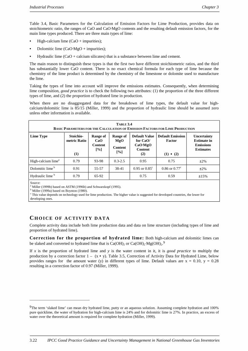
Industrial Processes Chapter 3
IPCC Good Practice Guidance and Uncertainty Management in National Greenhouse Gas Inventories3.22
Table 3.4, Basic Parameters for the Calculation of Emission Factors for Lime Production, provides data onstoichiometric ratio, the ranges of CaO and CaO·MgO contents and the resulting default emission factors, for themain lime types produced. There are three main types of lime:
• High-calcium lime (CaO + impurities);
• Dolomitic lime (CaO·MgO + impurities);
• Hydraulic lime (CaO + calcium silicates) that is a substance between lime and cement.
The main reason to distinguish these types is that the first two have different stoichiometric ratios, and the thirdhas substantially lower CaO content. There is no exact chemical formula for each type of lime because thechemistry of the lime product is determined by the chemistry of the limestone or dolomite used to manufacturethe lime.
Taking the types of lime into account will improve the emissions estimates. Consequently, when determininglime composition, good practice is to check the following two attributes: (1) the proportion of the three differenttypes of lime, and (2) the proportion of hydrated lime in production.
When there are no disaggregated data for the breakdown of lime types, the default value for high-calcium/dolomitic lime is 85/15 (Miller, 1999) and the proportion of hydraulic lime should be assumed zerounless other information is available.
TABLE 3.4BASIC PARAMETERS FOR THE CALCULATION OF EMISSION FACTORS FOR LIME PRODUCTION
Lime Type Stoichio-metric Ratio
(1)
Range ofCaO
Content[%]
Range ofMgO
Content[%]
Default Valuefor CaO/
CaO·MgOContent
(2)
Default EmissionFactor
(1) •••• (2)
UncertaintyEstimate inEmissionsEstimates
High-calcium limea 0.79 93-98 0.3-2.5 0.95 0.75 ±2%
Dolomitic lime b 0.91 55-57 38-41 0.95 or 0.85c 0.86 or 0.77c ±2%
Hydraulic lime b 0.79 65-92 0.75 0.59 ±15%
Source:a Miller (1999b) based on ASTM (1996b) and Schwarzkopf (1995).b Miller (1999a) based on Boynton (1980).c This value depends on technology used for lime production. The higher value is suggested for developed countries, the lower fordeveloping ones.
CH O I C E O F A C T I V I T Y D A T AComplete activity data include both lime production data and data on lime structure (including types of lime andproportion of hydrated lime).
Correction for the proportion of hydrated lime: Both high-calcium and dolomitic limes canbe slaked and converted to hydrated lime that is Ca(OH)2 or Ca(OH)2·Mg(OH)2.9
If x is the proportion of hydrated lime and y is the water content in it, it is good practice to multiply theproduction by a correction factor 1 – (x • y). Table 3.5, Correction of Activity Data for Hydrated Lime, belowprovides ranges for the amount water (y) in different types of lime. Default values are x = 0.10, y = 0.28resulting in a correction factor of 0.97 (Miller, 1999).
9The term ‘slaked lime’ can mean dry hydrated lime, putty or an aqueous solution. Assuming complete hydration and 100%pure quicklime, the water of hydration for high-calcium lime is 24% and for dolomitic lime is 27%. In practice, an excess ofwater over the theoretical amount is required for complete hydration (Miller, 1999).

Chapter 3 Industrial Processes
IPCC Good Practice Guidance and Uncertainty Management in National Greenhouse Gas Inventories 3.23
TABLE 3.5CORRECTION OF ACTIVITY DATA FOR HYDRATED LIME
Lime Type Theoretical Content of Water
in Hydrated Lime [%]
Content of Waterin Commercial
Hydrated Lime [%]
Default WaterContent Correction
Factor
High-calcium lime 24.3 26-28 0.28
Dolomitic lime 27.2 17-31 0.28
Hydraulic lime – – –
Source: Miller (1999b) based on ASTM (1996) and Schwarzkopf (1995).
CO M P L E T E N E S SCompleteness of the activity data (e.g. lime production) is a crucial attribute of good practice. Typically,reported production accounts for only a portion of the actual production, if lime production is considered to bethat product that is sold on the market. Use or production of lime as a non-marketed intermediate is not wellaccounted for or reported. For example, many plants that produce steel, synthetic soda ash, calcium carbide10,magnesia and magnesium metal, as well as copper smelters and sugar mills, produce lime but may not report it tonational agencies. Also, industries that regenerate lime from waste calcium carbonates (e.g. wood pulp and paperplants) are unlikely to report their lime production. Omission of these data may lead to an underestimation oflime production for a country by a factor of two or more.
DE V E L O P I N G A C O N S I S T E N T T I M E S E R I E SIt is good practice to calculate emissions from lime production using the same method for every year in the timeseries. Where data are unavailable to support a more rigorous method for all years in the time series, goodpractice is to recalculate these gaps according to the guidance provided in Chapter 7, Methodological Choice andRecalculation.
UN C E R T A I N T Y A S S E S S M E N TThe stoichiometric ratio is an exact number and therefore the uncertainty of the emission factor is the uncertaintyof lime composition, in particular of the share of hydraulic lime that has 15% uncertainty in the emission factor(2% uncertainty in the other types). Therefore, the total uncertainty is 15% at most (see Table 3.4, BasicParameters for the Calculation of Emission Factors for Lime Production).
The uncertainty for the activity data is likely to be much higher than for the emission factors, based on experiencein gathering lime data (see completeness section above). Omission of non-marketed lime production may lead toan error of +100% or more. The correction for hydrated lime typically adds about ±5% to the former uncertainty.
3.1.2.2 Reporting and documentationIt is good practice to document and archive all information required to produce the national emissions inventoryestimates as outlined in Chapter 8, Quality Assurance and Quality Control, Section 8.10.1, InternalDocumentation and Archiving. It is not practical to include all documentation in the national inventory report.However, the inventory should include summaries of methods used and references to source data such that thereported emissions estimates are transparent and steps in their calculation may be retraced.
To preserve an internally consistent emission time series, whenever national methods change, good practice is torecalculate the entire time series. If confidentiality is an issue for any type of production, estimates may beaggregated to the minimum extent possible to maintain confidentiality. 10 Some carbide producers may also regenerate lime from their calcium hydroxide by-products, which does not result inemissions of CO2. In making calcium carbide, quicklime is mixed with coke and heated in electric furnaces. The regenerationof lime in this process is done using a waste calcium hydroxide (hydrated lime) [CaC2 + 2 H2O → C2H2 + Ca(OH)2], notcalcium carbonate [CaCO3]. Thus, the calcium hydroxide is heated in the kiln to simply expel the water [Ca(OH)2 + heat →CaO + H2O] and no CO2 is released to the atmosphere.

Industrial Processes Chapter 3
IPCC Good Practice Guidance and Uncertainty Management in National Greenhouse Gas Inventories3.24
3.1.2.3 Inventory quality assurance/quality control (QA/QC)It is good practice to conduct quality control checks as outlined in Chapter 8, Quality Assurance and QualityControl, Table 8.1, Tier 1 General Inventory Level QC Procedures, and an expert review of the emissionsestimates. Additional quality control checks as outlined in Chapter 8, Section 8.7, Source Category-specific QCProcedures (Tier 2), and quality assurance procedures may also be applicable, particularly if higher tier methodsare used to determine emissions from this source category. Inventory agencies are encouraged to use higher tierQA/QC for key source categories as identified in Chapter 7, Methodological Choice and Recalculation.
In addition to the guidance in Chapter 8, specific procedures of relevance to this source category are outlinedbelow.
Comparison of the emissions est imates using different approaches
If the bottom-up approach is used, then inventory agencies should compare the emissions estimates to theestimate calculated using national lime production data (top-down approach). The results of such comparisonsshould be recorded for internal documentation, including explanations for any discrepancies.
Activity data check
Inventory agencies should confirm the correct definitions of the different types of lime produced in the country(i.e. CaO and MgO content, high-calcium quicklime (CaO), and dolomitic quicklime (CaO·MgO). They shouldcheck the completeness of national statistics for limestone, lime and dolomite use by comparing them with thedefault list of industries using limestone provided in the IPCC Guidelines, Vol. 3, p 2.9).

Chapter 3 Industrial Processes
IPCC Good Practice Guidance and Uncertainty Management in National Greenhouse Gas Inventories 3.25
3 . 1 . 3 I r o n a n d s t e e l i n d u s t r y
3.1.3.1 Methodological issuesCrude iron is produced by the reduction of iron oxide ores mostly in blast furnaces, generally using the carbon incoke or charcoal (sometimes supplemented with coal or oil) as both the fuel and reductant. In most iron furnaces,the process is aided by the use of carbonate fluxes (limestone). Additional emissions occur as the limestone ordolomite flux gives off CO2 during reduction of pig iron in the blast furnace, but this source category is coveredas emissions from limestone use (see the IPCC Guidelines, Vol. 3, Section 2.5, Limestone and Dolomite Use).Except for a small amount of carbon retained in the crude iron, all the carbon in the coke and in the fluxes isemitted as the product of combustion and calcination. Emissions also occur to a much lesser extent during theproduction of steel that is essentially the process of removal (generally by oxidation) of most of the carbon incrude iron.
Carbon plays the dual role of fuel and reductant. It is important not to double-count the carbon from theconsumption of coke or other reducing agents if this is already accounted for as fuel consumption in the EnergySector. Since the primary purpose of carbon oxidation is to reduce iron oxide ore to crude or pig iron (carbon isused as a reducing agent), the emissions are considered to be industrial processes emissions, and they should bepreferably reported as such. If this is not the case, it should be explicitly mentioned in the inventory. This sourcecategory should include CO2 emissions from the use of blast furnace gas as a fuel if emissions are reported in theIndustrial Processes Sector.
CH O I C E O F M E T H O DThe IPCC Guidelines outline several approaches for calculating CO2 emissions from iron and steel production.The choice of a good practice method depends on national circumstances as shown in the decision tree in Figure3.3, Decision Tree for the Iron and Steel Industry. The Tier 1 method calculates emissions from the consumptionof the reducing agent (e.g. coke from coal, coal, petroleum coke), using emission factors similar to those used toestimate combustion emissions. The Tier 1 method is rather simple and slightly overestimates emissions. TheTier 2 method is similar to Tier 1 but includes a correction for the carbon stored in the metals produced. Inaddition, a very simple approach that is mentioned in the IPCC Guidelines, is to multiply iron and steelproduction by a production-based emission factor. However, this method is not considered to be good practice.
CO2 emissions from limestone used as ‘flux’ in the reduction process are not included here because they areaccounted for in the IPCC Guidelines, Vol. 3, Section 2.5, Limestone and Dolomite Use.11
Tier 2 MethodThe Tier 2 method is based on tracking carbon through the production process. It is more accurate than Tier 1,but also more data-intensive. Estimating the emissions on the basis of plant-specific data for both Tier 1 and Tier2 will avoid double counting or missing emissions. With the Tier 2 method, emissions from iron production andsteel production are calculated separately. To achieve the highest accuracy, good practice is to develop emissionsestimates at the plant-level because plants can differ substantially in their technology. If plant-level data are notavailable, good practice is to use nationally compiled production data for iron/steel production that are to besubtracted from the fuel combustion sector. Thus, detailed knowledge of the conventions in the national energystatistics and the inventory are necessary to avoid double counting or omission.
Iron: Good practice is to use the following equation from the IPCC Guidelines:
EQUATION 3.6AEmissionspig iron = Emission Factor reducing agent • Mass of Reducing Agent + (Mass of Carbon in
the Ore – Mass of Carbon in the Crude Iron) • 44 / 12
11 Iron furnaces require limestone of higher purity than can be needed for clinker (cement) production. The IPCC Guidelinescite a USEPA reference that assumes 250 kg of lime is used for every tonne of iron. This value varies with the purity of oreand type of furnace, however.

Industrial Processes Chapter 3
IPCC Good Practice Guidance and Uncertainty Management in National Greenhouse Gas Inventories3.26
Reducing agents can be coke, coal, charcoal and petroleum coke. In Table 3.6, CO2 Emission Factors for MetalProduction (tonne CO2/tonne reducing agent), default emission factors from the IPCC Guidelines (Vol. 3, Table2-12, CO2 Emission Factors for Metal Production Generally (tonne CO2/tonne reducing agent)) are presented forthe most common reducing agents. In direct reduction techniques, other reducing agents such as CO, H2 ornatural gas are used. Plant-level or country-specific emission factors should be applied in these cases. Accordingto the IPCC Guidelines, CO2 emissions occurring from the limestone flux are reported as emissions fromlimestone and dolomite use (see the IPCC Guidelines, Vol. 3, Section 2.5, Limestone and Dolomite Use).
The amount of carbon in ore is almost zero and crude iron contains about 4% carbon.
Steel: Emissions from steel production (e.g. using a basic oxygen furnace (BOF), open hearth furnace (OHF) orelectric arc furnaces (EAF)) are based on the difference between the carbon contents of iron (3-5%) and steel(0.5-2%). In addition, for steel produced in electric arc furnaces it is good practice to add the carbon releasedfrom consumed electrodes to the emissions (roughly 1-1.5 kg carbon per tonne of steel):12
EQUATION 3.6BEmissions crude steel = (Mass of Carbon in the Crude Iron used for Crude Steel Production – Mass of Carbon in the Crude Steel) • 44 / 12
+ Emission FactorEAF • Mass of Steel Produced in EAF
The total emissions from iron and steel production are just the sum of the two Equations 3.6A and 3.6B above:
EQUATION 3.7Total emissions = Emissions pig iron + Emissions crude steel
Tier 1 MethodUsing the Tier 1 method, the carbon storage in pig iron and crude steel produced is not included as it is in theTier 2 method. This simplifies the calculation in the sense that the carbon content information in the metalsproduced is not required. When using the Tier 1 method, it is good practice to calculate the emissions as follows:
EQUATION 3.8Emissions = Mass of Reducing Agent •••• Emission Factor reducing agent
The coke and charcoal consumption in the iron and steel industry can be used to estimate the mass of reducingagents, if plant-specific information on the fuels used as reducing agent is not readily available (while subtractingthe same amount from the fuel combustion sector). This step affects only the sectoral allocation of the CO2emissions, not the total amount. The error made in neglecting the carbon storage term of Tier 2 will be 1-5% if allpig iron produced is used for the production of crude steel and at maximum 10% if all pig iron is used for otherpurposes (e.g. in cast iron foundries). Thus, this method will result in a small overestimation of the source.
12 Lime is added to electric arc furnaces (EAF) and its CO2 emission should be accounted for in the lime use section (see theIPCC Guidelines, Vol. 3, Section 2.5). The carbon emissions factor is based on carbon loss from the electrode as an averagevalue for the following process: In the EAF, the electrodes are made of carbon – either graphite or as Søderberg paste. Wherethe electrodes are kept above the steel melt (liquid), the electrical arc oxidises the carbon to CO or CO2. The rate of gasproduction will vary with the electrode type and various other factors. Also, the heat causes oxidation of carbon in the melt,reducing it from around 4% for crude iron to 2% or less (usually less than 1%) in steel. Sometimes, the electrode is immersedin the melt to increase the carbon content of the steel, should too much carbon have been burned out of the melt. In this case,carbon is removed from the electrode, but may or may not result in CO2 production. If the EAF is adjusted correctly, justenough electrode erosion is allowed to restore the steel’s carbon content to the desired level. If the EAF is not efficient,excess working electrode erosion happens to excess, the electrode is retracted to above the melt, and excess carbon in themelt is burned off.

Chapter 3 Industrial Processes
IPCC Good Practice Guidance and Uncertainty Management in National Greenhouse Gas Inventories 3.27
F i g u r e 3 . 3 D e c i s i o n T r e e f o r t h e I r o n a n d S t e e l I n d u s t r y
Isthere iron or
steel productionin the
country?
Yes
Report‘Not Occurring’
No
Aredata for
reducing agentsavailable?
Isthis a key
source category?(Note 1)
Estimateemissions using
the Tier 1 method
Estimateemissions using
the Tier 2 method
Obtain datafor reducing
agents
Calculate emissionsbased on mass of
reducing agent in pigiron production
Subtract carbon storagein the remaining iron
and in steel fromcalculated emissions
For any steel productionin electric arc furnaces,
add emissions fromburning electrodes
Subtract fuels used asreducing agents from theFuel Combustion sector
(includingblast furnace gas)
Use coke and charcoalconsumption in iron andsteel industry to estimate
the mass of reducing agent
Estimate emissionsbased of mass of
reducing agent in pigiron production
Subtract fuels used asreducing agents from theFuel Combustion sector
(includingblast furnace gas)
No
Yes
No
Box 2
Box 1
Note 1: A key source category is one that is prioritised within the national inventory system because its estimate has a significantinfluence on a country’s total inventory of direct greenhouse gases in terms of the absolute level of emissions, the trend in emissions, orboth. (See Chapter 7, Methodological Choice and Recalculation, Section 7.2, Determining National Key Source Categories.)
Note 2: CO2 emissions from limestone used as ‘flux’ in the reduction process are not included here since they are accounted for in theIPCC Guidelines, Vol. 3, section 2.5, on CO2 emissions from limestone and dolomite use.

Industrial Processes Chapter 3
IPCC Good Practice Guidance and Uncertainty Management in National Greenhouse Gas Inventories3.28
CH O I C E O F E M I S S I O N F A C T O R SIf country-specific data at the plant level are not available, the default emission factors for reducing agents in thepig iron production can be taken from the IPCC Guidelines, Vol. 3, Table 2-12 (see Table 3.6, CO2 EmissionFactors for Metal Production (tonne CO2/tonne reducing agent)).
TABLE 3.6CO2 EMISSION FACTORS FOR METAL PRODUCTION (TONNE CO2/TONNE REDUCING AGENT)
Reducing Agent Emission Factora
Coalb 2.5
Coke from coalb 3.1
Petrol coke 3.6a If better information on actual carbon content is not available nationally or cannot be calculated from data in the IPCC Guidelines, Vol.3, Chapter 1.b Derived from data in the IPCC Guidelines, Vol. 3, Chapter 1.
Source: IPCC Guidelines, Reference Manual, Table 2-12.
In direct reduction techniques, other reducing agents such as CO, H2 or natural gas are used, each with a specificemission factor. It is good practice to use plant specific emission factors for steel produced in an EAF. If plant-level data are not available, a default emission factor for the electrode oxidation should be used. For the Tier 2method, a default emission factor of 5 kg CO2 per tonne of steel produced in EAFs should be used for theelectrode consumption from the steel produced in electric arc furnaces (emission factorEAF ) (Tichy, 1999).
CH O I C E O F A C T I V I T Y D A T A
Tier 2 MethodActivity data should be collected at the plant-level. The most important datum is the amount of reducing agentused for iron production. If this is not a key source category and plant-specific data are not available, the mass ofreducing agent can be estimated using the Tier 1 approach (see below). In addition, the amount of pig ironproduced as well as the amounts used for crude steel production, and their carbon contents, should be collectedalong with data on the amount of crude steel produced in EAFs and the amount of iron in ore and its carboncontent.
Tier 1 MethodThe Tier 1 method requires only the amount of reducing agent used for iron production. If plant-specific data onthe mass of reducing agent are not available, they can be estimated by subtracting the amount of fuel used in theiron and steel industry (ISIC 1990) for the iron ore reduction from the fuel use and reported in the Energy Sector.The amount of fuel used for the reduction can be calculated from the mass balance of the chemical formula toreduce iron ore. This rough estimation affects only the allocation of the CO2 emissions between the IndustrialProcesses and the Energy Sector.
CO M P L E T E N E S SIn estimating emissions from this source category, there is a risk of double-counting or omission in either theIndustrial Processes or the Energy Sector. Since the primary use of coke oxidation is to produce pig iron, theemissions are considered to be industrial processes, and it should be reported as such. If this is not the case itshould be explicitly mentioned in the inventory. Inventory agencies should perform a doublecounting/completeness check. This will require good knowledge of the inventory in that source category.
DE V E L O P I N G A C O N S I S T E N T T I M E S E R I E SEmissions from iron and steel production should be calculated using the same method for every year in the timeseries. Where data are unavailable to support a more rigorous method for all years in the time series, these gapsshould be recalculated according to the guidance provided in Chapter 7, Methodological Choice andRecalculation.

Chapter 3 Industrial Processes
IPCC Good Practice Guidance and Uncertainty Management in National Greenhouse Gas Inventories 3.29
UN C E R T A I N T Y A S S E S S M E N TFor both Tier 1 and 2 the most important type of activity data is the amount of reducing agent used for ironproduction. According to Chapter 2, Energy, energy data have a typical uncertainty of about 5% (about 10% forcountries with less developed energy statistics). For calculating the carbon storage term Tier 2 requires additionalactivity data on amounts of pig iron and net crude steel production that have a typical uncertainty of a fewpercent. In addition, Tier 2 requires information on the carbon content of pig iron, crude steel, and of iron orethat may have an uncertainty of 5% when plant-specific data are available. Otherwise the uncertainty in thecarbon content could be of the order of 25 to 50%. Finally, the uncertainty in the emission factors for thereducing agent (e.g. coke) are generally within 5% (see Section 2.1.1.6, CO2 Emissions from StationaryCombustion, Uncertainty Assessment).
The systematic error made in emissions estimated in Tier 1 by neglecting the carbon storage term of Tier 2 willbe 1-5% if all pig iron produced is used for the production of crude steel and at maximum 10% if all pig ironshould be used for other purposes, i.e. in cast iron foundries. Thus, this method will result in a smalloverestimation of the source.
3.1.3.2 Reporting and documentationIt is good practice to document and archive all information required to produce the national emissions inventoryestimates as outlined in Chapter 8, Quality Assurance and Quality Control, Section 8.10.1, InternalDocumentation and Archiving. It is not practical to include all documentation in the national inventory report.However, the inventory should include summaries of methods used and references to source data such that thereported emissions estimates are transparent and steps in their calculation may be retraced.
Tier 2 MethodGood practice is to document the emissions, all activity data (reducing agents, carbon stored, steel produced inEAFs, electrodes), in addition to corresponding emission factors and assumptions used to derive them. Thereshould be an explanation of the linkage with the Fuel Combustion Sub-sector estimate to demonstrate that doublecounting or missing emissions have not occurred.
Tier 1 MethodBesides the emissions, good practice is to report the amount of reducing agents and their emission factors. In thecorresponding table, reported emissions are only part of total emissions and the rest are reported elsewhere (FuelCombustion Section).
In addition, inventory agencies should for both tiers, document all information needed to reproduce the estimate,as well as the QA/QC procedures.
3.1.3.3 Inventory quality assurance/quality control (QA/QC)It is good practice to conduct quality control checks as outlined in Chapter 8, Quality Assurance and QualityControl, Table 8.1, Tier 1 General Inventory Level QC Procedures, and an expert review of the emissionsestimates. Additional quality control checks as outlined in Chapter 8, Section 8.7, Source Category-specific QCProcedures (Tier 2), and quality assurance procedures may also be applicable, particularly if higher tier methodsare used to determine emissions from this source. Inventory agencies are encouraged to use higher tier QA/QCfor key source categories as identified in Chapter 7, Methodological Choice and Recalculation.
In addition to the guidance in Chapter 8, specific procedures of relevance to this source category are outlinedbelow.
Activity data check
For the Tier 2 method, inventory agencies should check with Fuel Combustion as mentioned in Section 2.1.1.4 toensure that emissions from heating/reducing agents (coal, coke, natural gas, etc.) are not double counted oromitted.
Inventory agencies should examine any inconsistency between data from different plants to establish whetherthese reflect errors, different measurement techniques or result from real differences in emissions, operationalconditions or technology. This is particularly relevant to the plant-specific estimates of the mass of the reducingagent.

Industrial Processes Chapter 3
IPCC Good Practice Guidance and Uncertainty Management in National Greenhouse Gas Inventories3.30
Inventory agencies should compare aggregated plant-level estimates to industry totals for carbon and limestoneconsumption where such trade data are available.

Chapter 3 Industrial Processes
IPCC Good Practice Guidance and Uncertainty Management in National Greenhouse Gas Inventories 3.31
3 . 2 N 2 O E M I S S I O N S F R O M A D I P I C A C I D A N DN I T R I C A C I D P R O D U C T I O N
3 . 2 . 1 M e t h o d o l o g i c a l i s s u e sNitrous oxide (N2O) is generated as an unintended by-product during the production of adipic acid and nitric acid(HNO3), and in many industrial processes that use nitrogen oxides or nitric acids as feedstocks (e.g. themanufacture of caprolactam, glyoxal, and nuclear fuel reprocessing). Adipic acid and nitric acid are large sourcesof atmospheric N2O if not abated.13 Emissions of N2O from these processes depend on the amount generated inthe specific production process and the amount destroyed in any subsequent abatement process. Abatement ofN2O can be intentional, through installation of equipment specifically designed to destroy N2O in adipic acidplants, or unintentional in systems designed to abate other emissions such as nitrogen oxides (NOx). For furtherdiscussion, see Reference Manual of the IPCC Guidelines (Sections 2.9 and 2.10, Nitric Acid Production andAdipic Acid Production).
CH O I C E O F M E T H O DThe choice of good practice methods depends on national circumstances. The decision tree in Figure 3.4,Decision Tree for N2O Emissions from Adipic Acid and Nitric Acid Production describes good practice inadapting the methods in the IPCC Guidelines to these national circumstances. The decision tree should beapplied separately to adipic and nitric acid production.
The IPCC Guidelines present a basic equation for estimating N2O emissions in which production data ismultiplied by an emission factor. Given the current and potential future use of N2O abatement technologies,particularly in adipic acid plants, it is good practice to include an additional term in this equation as follows:
EQUATION 3.9N2O Emissions = Specific Emission Factor • Production Level • [1 – (N2O Destruction Factor
• Abatement System Utilisation Factor)]
The N2O destruction factor has to be multiplied by an abatement system utility factor in order to account for anydown time of the emission abatement equipment (i.e. time the equipment is not operating).
To achieve the highest accuracy, good practice is to apply this equation at the plant-level using N2O generationand destruction factors developed from plant-specific measurement data. In this case, the national total is equal tothe sum of plant totals. Where plant-level information is not available, good practice provides default N2Ogeneration factors and destruction factors as shown in Tables 3.7, Default Factors for Adipic Acid Production,and 3.8, Default Factors for Nitric Acid Production, based on the plant types and abatement technologiesimplemented.
Given the relatively small number of adipic acid plants (about 23 globally, Choe et al., 1993), obtaining plant-specific information requires few additional resources. However, there are more nitric acid plants (estimatesrange from 255 to 600 plants according to Choe et al., 1993,, Bockman and Granli, 1994) with a much greatervariation in the N2O generation factors among plant types. Thus, default factors may be needed more often fornitric acid N2O emissions estimates. Where default values are used to estimate emissions from nitric acidproduction, it is good practice to categorise plants according to type and to use an appropriate N2O generationfactor used to the extent possible.
13 The chemical and other industries included in this section are generally unrelated except for the fact that nitric acid is usedin the manufacture of adipic acid. The manufacturing technologies and the applicable technologies for abating N2O are verydifferent for each industry.

Industrial Processes Chapter 3
IPCC Good Practice Guidance and Uncertainty Management in National Greenhouse Gas Inventories3.32
F i g u r e 3 . 4 D e c i s i o n T r e e f o r N 2 O E m i s s i o n s f r o m A d i p i c A c i d a n dN i t r i c A c i d P r o d u c t i o n
Arethere adipic or
nitric acid plants inthe country?
Areemissions
and destruction dataavailable directly
from plants?
Report‘Not Occurring’
Is thisa key source
category, and is nitricacid/adipic acid a significant
sub-source category?(Note 1 and
Note 2)
Areplant-specific
production dataavailable?
Areaggregate production
data available?
Areplant-specific
emission factorsavailable?
Use industry suppliedemission estimates with
appropriate QA/QC,audits and review
Collect emission anddestruction data
directly from plants
Calculate emissionsusing plant-specificfactors, and subtract
destruction
Gather data oruse productioncapacity default
data
Multiplyproduction by
default emissionfactors
Calculate emissionsusing default factors,
and subtractdestructionBox 1
No
Yes
Box 2
No
Yes
Box 4
No
Yes
Box 3
No
No
YesYes
No
Note 1: A key source category is one that is prioritised within the national inventory system because its estimate has a significantinfluence on a country’s total inventory of direct greenhouse gases in terms of the absolute level of emissions, the trend in emissions, orboth. (See Chapter 7, Methodological Choice and Recalculation, Section 7.2, Determining National Key Source Categories.)
Note 2: As a rule of thumb, a sub-source category would be significant if it accounts for 25-30% of emissions from the source category.

Chapter 3 Industrial Processes
IPCC Good Practice Guidance and Uncertainty Management in National Greenhouse Gas Inventories 3.33
CH O I C E O F E M I S S I O N F A C T O R SPlant measurements provide the most rigorous data for calculating net emissions (i.e. N2O generation anddestruction factors). Monitoring N2O emissions from both adipic acid and nitric acid production is practicalbecause these are point sources and there are a finite number of production plants. Given currently availabletechnology, instrumentation for sampling and monitoring emission rates do not limit precision or accuracy of theoverall measurement. Usually sampling frequency and timing is sufficient to avoid systematic errors and toachieve the desired level of accuracy. As a general rule, it is good practice to conduct sampling and analysiswhenever a plant makes any significant process changes that would affect the generation rate of N2O, andsufficiently often otherwise to ensure that operating conditions are constant. In addition, plant operators shouldbe consulted annually to determine the specific destruction technologies employed and confirm their use, sincetechnologies may change over time. Precise measurement of the emissions rate and abatement efficienciesrequires measurement of both the exit stream and the uncontrolled stream. Where measurement data are availableonly on the exit stream, good practice is to base emissions on these data. In this case, any available estimates ofabatement efficiency should be provided only for information purposes and not used to calculate emissions.
If plant-level factors are not available, it is good practice to use default factors. These default values oftenrepresent midpoint or mean values of data sets (as determined by expert analysis). The extent to which theyrepresent a specific plant’s emission rate is unknown. Default factors should be used only in cases where plant-specific measurements are not available.
Table 3.7, Default Factors for Adipic Acid Production, presents default emission factors for adipic acidproduction, and default N2O destruction factors for commonly used abatement technologies, and associateduncertainties. This table supplements the IPCC Guidelines default values by providing information about N2Oabatement technologies. Failure to determine if abatement technologies are being used can result inoverestimation of emissions.
Table 3.8, Default Factors for Nitric Acid Production, supplements the emission factors for nitric acid productionprovided in the IPCC Guidelines (Vol. 3, Section 2.9, Table 2-7, Emission Factors for N2O from Nitric AcidProduction). It also includes additional emission and destruction factors for NOx abatement technologies, andassociated uncertainties. The generation factors listed in Table 3.8 for plants using non-selective catalyticreduction (NSCR) already incorporate the effect of abatement measures. The N2O destruction factor for NSCR inTable 3.8 is provided for information purposes only and should not be applied to an emissions estimate using theNSCR default generation factor because this would double-count the destruction.
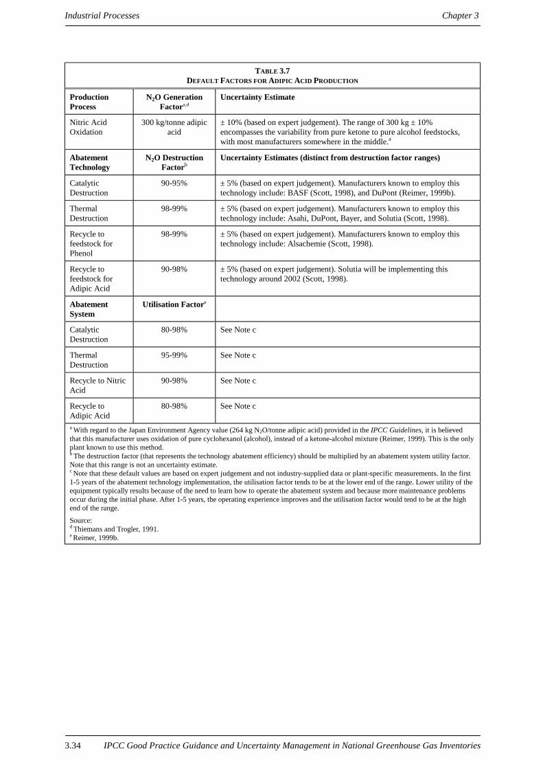
Industrial Processes Chapter 3
IPCC Good Practice Guidance and Uncertainty Management in National Greenhouse Gas Inventories3.34
TABLE 3.7DEFAULT FACTORS FOR ADIPIC ACID PRODUCTION
ProductionProcess
N2O GenerationFactora,d
Uncertainty Estimate
Nitric AcidOxidation
300 kg/tonne adipicacid
± 10% (based on expert judgement). The range of 300 kg ± 10%encompasses the variability from pure ketone to pure alcohol feedstocks,with most manufacturers somewhere in the middle.a
AbatementTechnology
N2O DestructionFactorb
Uncertainty Estimates (distinct from destruction factor ranges)
CatalyticDestruction
90-95% ± 5% (based on expert judgement). Manufacturers known to employ thistechnology include: BASF (Scott, 1998), and DuPont (Reimer, 1999b).
ThermalDestruction
98-99% ± 5% (based on expert judgement). Manufacturers known to employ thistechnology include: Asahi, DuPont, Bayer, and Solutia (Scott, 1998).
Recycle tofeedstock forPhenol
98-99% ± 5% (based on expert judgement). Manufacturers known to employ thistechnology include: Alsachemie (Scott, 1998).
Recycle tofeedstock forAdipic Acid
90-98% ± 5% (based on expert judgement). Solutia will be implementing thistechnology around 2002 (Scott, 1998).
AbatementSystem
Utilisation Factore
CatalyticDestruction
80-98% See Note c
ThermalDestruction
95-99% See Note c
Recycle to NitricAcid
90-98% See Note c
Recycle toAdipic Acid
80-98% See Note c
a With regard to the Japan Environment Agency value (264 kg N2O/tonne adipic acid) provided in the IPCC Guidelines, it is believedthat this manufacturer uses oxidation of pure cyclohexanol (alcohol), instead of a ketone-alcohol mixture (Reimer, 1999). This is the onlyplant known to use this method.b The destruction factor (that represents the technology abatement efficiency) should be multiplied by an abatement system utility factor.Note that this range is not an uncertainty estimate.c Note that these default values are based on expert judgement and not industry-supplied data or plant-specific measurements. In the first1-5 years of the abatement technology implementation, the utilisation factor tends to be at the lower end of the range. Lower utility of theequipment typically results because of the need to learn how to operate the abatement system and because more maintenance problemsoccur during the initial phase. After 1-5 years, the operating experience improves and the utilisation factor would tend to be at the highend of the range.
Source:d Thiemans and Trogler, 1991.e Reimer, 1999b.

Chapter 3 Industrial Processes
IPCC Good Practice Guidance and Uncertainty Management in National Greenhouse Gas Inventories 3.35
TABLE 3.8DEFAULT FACTORS FOR NITRIC ACID PRODUCTION
Production Process N2O GenerationFactor
(kg N2O/tonnenitric acid)
Special Considerations
Canada
- plants without NSCRa
8.5 Based on an average emissions rate for plants of European design(Collis, 1999)
- plants using NSCR <2 The N2O generation factor accounts for N2O destruction by NSCR.Uncertainty = ± 10% (based on expert judgement – Collis, 1999).
USA
- plants without NSCR
9.5 An estimated 80% of nitric acid (HNO3) plants do not use NSCRsystems (Choe et al., 1993).
- plants using NSCR 2 The N2O generation factor accounts for N2O destruction by NSCR.Industry indicates a range of 1.12 to 2.5 kg N2O/tonne HNO3, fieldexperts have indicated that the lower end of the range is moreaccurate (Choe et al., 1993,, Collis, 1999). A factor of 2 wasselected as a conservative default. An estimated 20% of HNO3plants use NSCR systems (Choe et al., 1993). Uncertainty = ±10% (based on expert judgement).
Norway
- process-integrated N2Odestruction
<2 Norsk Hydro developed a state-of-the-art reactor design in whichemissions of N2O are reduced in a process-integrated manner(Norsk Hydro, 1996). There is only one installation operational ofthis type (Oonk, 1999).
- atmospheric pressure plant(low pressure)
4-5 (Norsk Hydro, 1996)
- medium pressure plant 6-7.5 (Norsk Hydro, 1996)
Japan 2.2-5.7 (Japan Environment Agency, 1995)
Other Countries
- European designed, dualpressure, double absorptionplants
8-10
- Older (pre - 1975), plantswithout NSCR
10-19 Emission factors up to 19 kg N2O/tonne nitric acid have beenreported for plants not equipped with NSCR technology (Choe etal., 1993, EFMA, 1995). Such a high emissions rate would mostlikely apply to outdated plants (Choe 1993, Cook (1999).
NOx AbatementTechnology
N2O DestructionFactor (%)
Notes
Non-Selective CatalyticReduction (NSCR)
80-90 Uncertainty = ± 10% (based on expert judgement). NSCR is atypical tail gas treatment in the USA and Canada with lessapplication in other parts of the world.
Selective CatalyticReduction (SCR)
0 SCR with ammonia does not reduce N2O.
Extended Absorption 0aNon-Selective Catalytic Reduction (NSCR).

Industrial Processes Chapter 3
IPCC Good Practice Guidance and Uncertainty Management in National Greenhouse Gas Inventories3.36
CH O I C E O F A C T I V I T Y D A T AIt is good practice to gather activity (production) data at a level of detail consistent with that of the generationand destruction data. Where plant-level emission factors are used, good practice is to collect plant-levelproduction data. Typical plant-level production data is accurate to ±2% due to the economic value of havingaccurate information . If plant-level data are not available, nationally compiled production data may be used.However, for the nitric acid source category, these statistics may miss an average of one-half of a national total(see details in Completeness Section).
If neither plant-level nor national-level activity data are available, information on production capacity can beused. It is good practice to multiply the total national production capacity by a capacity utilisation factor of 80%± 20% (i.e. range of 60-100%).
CO M P L E T E N E S SComplete coverage for the adipic acid source category is straightforward, but nationally compiled nitric acidproduction statistics may miss an average of one-half of the total. Studies that compare global statistics compiledfrom national data on nitric acid production with industry estimates of global production suggest that the nationalstatistics account for only 50 to 70% of the total (Bouwman et al., 1995, Olivier, 1999). This is probably due tonitric acid production that is integrated as part of larger production processes, where the nitric acid never entersinto commerce and is not counted in the national statistics. For example, in the manufacture of caprolactam,nitrogen oxides produced via ammonia oxidation are used directly in the process without prior conversion tonitric acid. Accounting for these sources by methods such as identifying them through national registries of NOxemissions, another unintended by-product of nitric acid production, will improve completeness.
DE V E L O P I N G A C O N S I S T E N T T I M E S E R I E SN2O emissions should be recalculated for all years whenever emission calculation methods are changed (e.g. ifthe inventory agency changes from the use of default values to actual values determined at the plant level). Ifplant-specific data are not available for all years in the time series, it will be necessary to consider how currentplant measurements can be used to recalculate emissions for previous years. It may be possible to apply currentplant-specific emission factors to production data from previous years, provided that plant operations have notchanged substantially. Such a recalculation is required to ensure that any changes in emissions trends are real andnot an artefact of changes in procedure. It is good practice to recalculate the time series according to theguidance provided in Chapter 7, Methodological Choice and Recalculation.
UN C E R T A I N T Y A S S E S S M E N TUncertainties for the default values are estimates based on expert judgement. In general, adipic acid defaultemission factors are more certain than nitric acid default emission factors because they are derived from thestoichiometry of an intended chemical reaction (nitric acid oxidation) and N2O-specific abatement systems. Theuncertainty in the emission factor for adipic acid represents a variability in N2O generation due to differences inthe composition of the cyclohexanone and cyclohexanol feedstock (i.e. ketone and alcohol) that are used bydifferent manufacturers. Higher ketone content results in increased N2O generation, whereas higher alcoholcontent results in less N2O generation (Reimer, 1999a). An individual plant should be able to determine theproduction of N2O (based on HNO3 consumption) within 1%. In contrast, the default values for nitric acidproduction are much more uncertain. First, N2O may be generated in the gauze reactor section of nitric acidproduction as an unintended by-product reaction (Cook, 1999). Second, the exhaust gas may or may not betreated for NOx control, and the NOx abatement system may or may not reduce (or may even increase) the N2Oconcentration of the treated gas. 14
Although there is greater uncertainty associated with nitric acid values than those for adipic acid, potential N2Oemissions per metric ton produced are far greater for adipic acid production. Thus, the uncertainty associatedwith adipic acid production may be more significant when converted into N2O emissions. A properly maintainedand calibrated monitoring system can determine emissions using Equation 3.9 above to within ±5% at the 95%confidence level.
14 In some cases, processes designed to reduce NOx emissions may result in additional N2O generation. Increased N2Oconcentrations due to NOx abatement technology have been measured at various power plants that employ non-catalyticreduction for NOx (Cook, 1999). From at least one nitric acid plant, it is known that NOx control resulted in increased N2Oemissions (Burtscher, 1999).
Chapter 3 Industrial Processes
IPCC Good Practice Guidance and Uncertainty Management in National Greenhouse Gas Inventories 3.37
3 . 2 . 2 R e p o r t i n g a n d d o c u me n t a t i o nIt is good practice to document and archive allinformation required to produce the nationalemissions inventory estimates as outlined inChapter 8, Quality Assurance and QualityControl, Section 8.10.1, Internal Documentationand Archiving.
Some examples of specific documentation andreporting relevant to this source category areprovided below:
• Description of the method used;
• Number of adipic acid and nitric acid plants,respectively;
• Emission factors;
• Production data;
• Production capacity;
• Number of plants using abatementtechnology;
• Type of abatement technology, destruction efficiency, and utilisation;
• Any other assumptions.
Plant operators should supply this information to the inventory agency for compilation, and also archive theinformation at the site. Plant operators should also log and archive the measurement frequencies and instrumentalcalibration records where actual plant measurements are made.
Where there are only one or two producers in a country, as could often be the case for adipic acid production,activity data may be considered confidential. In this case, operators and the inventory agency should determinethe level of aggregation at which information can be reported while still protecting confidentiality. Detailedinformation including instrumentation records should still be archived at the plant level.
It is not practical to include all documentation in the national inventory report. However, the inventory shouldinclude summaries of methods used and references to source data such that the reported emissions estimates aretransparent and steps in their calculation may be retraced.
3 . 2 . 3 I n v e n t o r y q u a l i t y a s s u r a n c e / q u a l i t y c o n t r o l( Q A / Q C )
It is good practice to conduct quality control checks as outlined in Chapter 8, Quality Assurance and QualityControl, Table 8.1, Tier 1 General Inventory Level QC Procedures, and an expert review of the emissionsestimates. Additional quality control checks as outlined in Chapter 8, Section 8.7, Source Category-specific QCProcedures (Tier 2), and quality assurance procedures may also be applicable, particularly if higher tier methodsare used to determine emissions from this source category. Inventory agencies are encouraged to use higher tierQA/QC for key source categories as identified in Chapter 7, Methodological Choice and Recalculation.
In addition to the guidance in Chapter 8, specific procedures of relevance to this source category are outlinedbelow.
Comparison of emissions est imates using different approaches
If emissions are calculated using data from individual adipic acid and nitric acid plants (bottom-up approach),inventory agencies should compare the estimate to emissions calculated using national production data (top-downapproach). They should record the results and investigate any unexplained discrepancies.
Since industrial N2O source categories are relatively small compared to other anthropogenic and natural sources,it is not feasible to compare emissions with measured trends in atmospheric N2O concentrations.
BOX 3.1OTHER POTENTIAL INDUSTRIAL N2O SOURCES
The Reference Manual of the IPCC Guidelinesidentifies several other potential N2O sourcecategories of unknown magnitude, but which arebelieved to be small. Potential N2O non-combustion industrial source categories include:caprolactam production, urea production,petrochemical production, propellant and foamingagents, fumes from explosives, dodecanedioic acidproduction (DDDA or 3DA), and fume sweepfrom adipic acid and nitric acid tanks. Inventoryagencies that quantify such source categoriesshould report the data in their inventory andprovide documentation of their method. Thisinformation could provide a basis for subsequentrevisions of the IPCC Guidelines.

Industrial Processes Chapter 3
IPCC Good Practice Guidance and Uncertainty Management in National Greenhouse Gas Inventories3.38
Plant- level data
Inventory agencies should archive sufficient information to allow an independent review of the time series ofemissions beginning in the base year, and to explain trends in emissions when making historical comparisons.This is particularly important in cases where recalculations are necessary, for example, when an inventory agencychanges from using default values to actual values determined at the plant level.
Revision of direct emission measurements
If plant-level N2O measurements are available, inventory agencies should confirm that internationally recognised,standard methods were used. If the measurement practices fail this criterion, then they should evaluate the use ofthese emissions data. In addition, they should reconsider the uncertainty estimates in light of the QA/QC results.
Inventory agencies should compare plant-based factors to the IPCC defaults to ensure that the plant-specificfactors are reasonable. They should explain and document any differences between plant-specific factors anddefault factors, particularly any differences in plant characteristics that might lead to these differences.
Chapter 3 Industrial Processes
IPCC Good Practice Guidance and Uncertainty Management in National Greenhouse Gas Inventories 3.39
3 . 3 P F C E M I S S I O N S F R O M A L U M I N I U MP R O D U C T I O N
3 . 3 . 1 M e t h o d o l o g i c a l i s s u e sTwo PFCs, tetrafluoromethane (CF4), and hexafluoroethane (C2F6) are known to be emitted from the process ofprimary aluminium smelting. These PFCs are formed during the phenomenon known as the anode effect (AE),when the aluminium oxide concentration in the reduction cell electrolyte is low.
CH O I C E O F M E T H O DThe choice of a good practice method will depend on national circumstances. The decision tree in Figure 3.5,Decision Tree for PFC Emissions from Aluminium Production describes good practice in adapting the methodsin the IPCC Guidelines to these country-specific circumstances. The decision tree should be applied separatelyfor CF4 and C2F6 emissions estimation.
The IPCC Guidelines describe three general methods for estimating PFC emissions from aluminium production(Vol.3, Section 2.13.6, PFCs from Aluminium Production). These three methods correspond to tiers, but are notidentified as such. To be consistent with other sections of the IPCC Guidelines and the good practice guidance,the methods presented in the IPCC Guidelines are referred to as tiers in this section.
The most accurate method is either to monitor smelter emissions continuously (Tier 3a) or to develop a smelter-specific long term relationship between measured emissions and operating parameters and to apply thisrelationship using activity data (Tier 3b). The Tier 3b method requires comprehensive measurements to developthe smelter-specific relationship and on-going collection of operating parameter data (e.g. frequency and durationof anode effects and the Anode Effect Overvoltage15) and production data. Where a smelter-specific relationshiphas not been developed but information on operating parameters and production is available, default technology-specific slope and overvoltage coefficients may be used (Tier 2). Where the only information available is theannual quantity of aluminium produced, default emission factors by technology type may be used (Tier 1). Thelevel of uncertainty in the Tier 1 method will be much greater than for estimations produced using Tier 3 or Tier2 methods.
15 The Anode Effect Overvoltage indicates the fluctuation in voltage occurring during the anode effect.

Industrial Processes Chapter 3
IPCC Good Practice Guidance and Uncertainty Management in National Greenhouse Gas Inventories3.40
F i g u r e 3 . 5 D e c i s i o n T r e e f o r P F C E m i s s i o n s f r o m A l u m i n i u mP r o d u c t i o n
Is thereany aluminium
production in thecountry?
Areemissions
continuouslymonitored?
Report‘Not Occurring’
Are theresmelter-specific slope
or over-voltage coefficientsrelating process datato emission factors?
(Note 2)
Sumemissions
across plants
No
Yes
Box 4
No
Yes
Aresmelter level
process data available(AEF and AED,
or AEO)?
Is thisa key source
category?(Note 1)
Obtainprocess
data
Estimate smelter emissionsusing default coefficient in
Slope or Pechiney equation.Multiply by smelter
production over time.(Refer to Table 3.9)
Use defaultemission factors by
technology type(Refer to
Table 3.10)
Estimate smelter emissionsusing smelter-specificcoefficient in Slope or
Pechiney equation.Multiply by smelter
production over time.
Estimate smelteremissions multiplying
emission factor bysmelter production
over time
Yes
Yes
No No
Yes
No
Box 1Box 3
Box 2
Note 1: A key source category is one that is prioritised within the national inventory system because its estimate has a significantinfluence on a country’s total inventory of direct greenhouse gases in terms of the absolute level of emissions, the trend in emissions,or both. (See Chapter 7, Methodological Choice and Recalculation, Section 7.2, Determining National Key Source Categories.)
Note 2: In cases where a smelter has more than one distinct cell technology, a smelter must measure/use specific emission coefficientsfor each technology.

Chapter 3 Industrial Processes
IPCC Good Practice Guidance and Uncertainty Management in National Greenhouse Gas Inventories 3.41
Tier 3a Method – Continuous emission monitoringContinuous monitoring of emissions is possible and is the most accurate means of determining emissions. Givenlikely cost and other resource considerations, however, it is not regarded as necessary for good practice. Fordetails on direct measurement techniques, see Box 3.2, Direct Measurement Techniques, below.
BOX 3.2DIRECT MEASUREMENT TECHNIQUES
Sampling and measurement must be performed to a good practice standard to ensure the accuracyof the data, which means that:
• Measurements of PFCs at smelters should account for both emissions captured by the reductioncell hooding and extracted by the fume exhaust duct, and also fugitive emissions released intothe potroom16 atmosphere. Ideally, these data can be obtained by direct measurement of PFCsin duct and fugitive emissions. Otherwise, direct measurement of PFCs in duct emissions can beconducted along with careful measurement of the cell hooding capture efficiency, allowingfugitive emissions to be calculated.
• The analytical technology used should be capable of measuring both CF4 and C2F6 gasessimultaneously. Several suitable analytical technologies are available. The technology chosenmust have a suitable dynamic range for the measurement of expected concentrations of ductemissions and fugitive emissions. The sensitivity of the detection should be capable of reliablemeasurement at the lowest levels expected in electrolysis cell exhaust ducts and for fugitiveemissions where fugitive emissions account for 5% or more of total PFC emissions. Thedynamic range of the measurement device should be capable of reliable measurement to thehighest concentration to be measured. For duct emissions, this means a concentrationmeasurement range of 0 to 1000 ppmv (parts per million by volume). Measurements should benormalised for temperature and pressure and these measurement conditions must be reportedand recorded with the concentration measurements that will be used when calculating massemissions.
• Duct volumetric gas flow measurements should be performed according to nationally orinternationally recognised standards. Gas flow measurements should be performed during thecourse of the concentration measurement program at sufficient intervals to ensure accuraterepresentation of the volumetric gas flow. Measurements should be normalised for temperatureand pressure and these measurement conditions must be reported and recorded with the flowmeasurements that will be used when calculating mass emissions.
• Calibration of analytical instruments should be performed at regular intervals during themeasurement campaign. The required schedule for calibrations will vary according to the typeand known stability of the analytical instrumentation used but must be sufficient to minimise theeffect of instrument calibration drift. The results of all calibrations should be reported andrecorded with the concentration measurement. Measurements affected by drift should beomitted from emission estimations. Calibration gases should be traceable to recognised nationalor international standards. The calibration method should be thoroughly documented andrecorded with the emission measurements. Chapter 8, Quality Assurance and Quality Control,provides general advice on sampling representativeness.
16 The potroom is the standard industry term for the large room in which the reduction cells or ‘pots’ are housed. Thesmelting cells have hooding which, depending on the smelter design, age etc., will have varying fume collection efficiency.The collected fume is transported via ducts to a fume scrubbing facility where other pollutants are removed. Fume thatescapes from the hooding may either be collected in a fume manifold and also transported to the fume scrubbing facility orexhausted to atmosphere through the potroom roof. Since the potrooms may be up to a kilometre long and 20 metres or morein width, accurate measurements of fugitive emissions may not be feasible. Therefore, measurements of PFCs in collectedfume and fugitive fume are required or else measurements of collected fume along with a comprehensive understanding ofthe fume collection efficiency is required to ensure that PFCs captured by the scrubbing system along with fugitive emissionsare included in estimations.

Industrial Processes Chapter 3
IPCC Good Practice Guidance and Uncertainty Management in National Greenhouse Gas Inventories3.42
Tier 3b Method – Smelter-specif ic relationship between emissions andoperating parameters based on f ield measurementsThis method uses periodic measurements to establish a smelter-specific relationship between operatingparameters (i.e. frequency and duration of anode effects or Anode Effect Overvoltage) and emissions of CF4 andC2F6. Once established, the relationship can be used along with process data collected on an on-going basis, toestimate emissions factors over time. These emission factors are multiplied by smelter-specific production(tonnes) to estimate smelter emissions. Emissions estimates will be aggregated across smelters to estimatenational emissions.
The following estimation relationships can be used:
Slope Method: This method uses a linear least squares relationship between anode effect (AE) minutes percellday17 and emissions, expressed as an emission factor (EF):
EQUATION 3.10EF (kg CF4 or C2F6 per tonne of Al) = Slope • AE min / cellday
To develop an accurate estimate of the slope, simultaneous measurements of emissions and collection of anodeeffect data over an appropriate period of time are required. The Slope Method is a variant of the Tabereauxapproach described in the IPCC Guidelines:
BOX 3.3TABEREAUX APPROACH
Slope = 1.698 • (p / CE) and AE min / cellday = AEF • AED
Where:
p = Average fraction of CF4 in the cell gas during anode effects for the CF4 slope or the average fraction of C2F6 in the cell gas during anode effects for the C2F6 slope
CE = Current Efficiency for the aluminium production process
AEF = Number of anode effects per cellday
AED = Anode effect duration in minutes
Pechiney Overvoltage Method: This method uses the Anode Effect Overvoltage as the relevant processparameter. The Anode Effect Overvoltage is the extra cell voltage, above 8V, caused by anode effects, whenaveraged over a 24-hour period (mV/day). The correlation formula was derived from measurements of PFCgeneration at smelters with Pechiney technology, expressed as an emission factor (EF):
EQUATION 3.11EF (kg CF4 or C2F6 per tonne of Al) = Over-Voltage Coefficient • AEO / CE
Where:
AEO = Anode effect over-voltage in mV/cellday
CE = Aluminium production process current efficiency expressed as a fraction
Tier 2 Method – smelter-specif ic relationship between emissions & operatingparameters based on default technology-based slope and over-voltagecoeff icientsIf measurement data are not available to determine smelter-specific Slope or Overvoltage coefficients, defaultcoefficients may be used together with smelter-specific operating parameters. Good practice default coefficients
17 The ‘cellday’ term really means ‘the number of cells operating multiplied by the number of days of operation’. At asmelter this would more usually be calculated (for a certain period of time, e.g. a month or a year) using ‘the average numberof cells operating across the smelter over a certain period of days multiplied by the number of days in the period’.

Chapter 3 Industrial Processes
IPCC Good Practice Guidance and Uncertainty Management in National Greenhouse Gas Inventories 3.43
are listed in Table 3.9, Default Coefficients for the Calculation of PFC Emissions from Aluminium Production(Tier 2 Methods).
Tier 1 Method – Production-based emission factorsThe simplest estimation method is to multiply default emission factors by aluminium production. When the onlysmelter-specific activity data available are metal production statistics, it is good practice to use default emissionfactors (see Choice of Emission Factors).
Default slope coefficients (Tier 2 method) and emission factors (Tier 1 method) were developed using availabledata from International Primary Aluminum Institute (IPAI) surveys and other field measurement data (Bouzat etal., 1996, Leber et al., 1998, Marks, 1998, Roberts et al., 1994a and 1994b, Kimmerle et al., 1998, Marks et al.,2000). The limited information available for some data required expert judgement regarding the suitability ofsome measurement sets. As an example, the Tier 1 Method Horizontal Stud Søderberg (HSS) default emissionfactors were calculated using 1991 data, rather than 1990 data.
When possible, the consistency of available measurement data surveyed over different time periods and atdifferent smelters should be used to confirm a significant degree of confidence about the magnitude and trend ofthe emission factors and coefficients.
CH O I C E O F E M I S S I O N F A C T O R S
Tier 3b MethodFor this method, it is good practice to determine the coefficients of the models by using smelter-specificmeasurements. The smelter-specific coefficients should be based on comprehensive measurements of CF4 andC2F6 emissions with simultaneous collection of process data. This means that emission factors should reflect thespecific conditions of a plant and the technologies involved. Emission factors are to be measured over a period oftime that reflects the variability of the process and accounts for both emissions captured by the fume collectionsystem and fugitive emissions (if this sub-source category is significant, compared with emissions captured by thefume control system). Box 3.2, Direct Measurement Techniques, gives guidance on some aspects of directmeasurement techniques. It is good practice to follow these approaches in implementing a sampling andmeasurement program.18
Tier 2 MethodIf smelter-specific measurements are unavailable, default coefficients may be used. Default coefficients areprovided by technology type in Table 3.9, Default Coefficients for the Calculation of PFC Emissions fromAluminium Production (Tier 2 Methods).19 The default coefficients must be applied by technology type withineach smelter. If more than one technology type is being used at a smelter, the appropriate default coefficientsmust be applied separately for each technology segment.
18 Other methods may incorporate an explicit factor representing a contribution from newly started cells. The smelter-specific slope coefficients developed under Tier 3b will incorporate these emissions.
19 Current measurement programs are improving the quantity and quality of available data. These data should be available byearly 2000, and may supersede the values provided in Table 3.9.
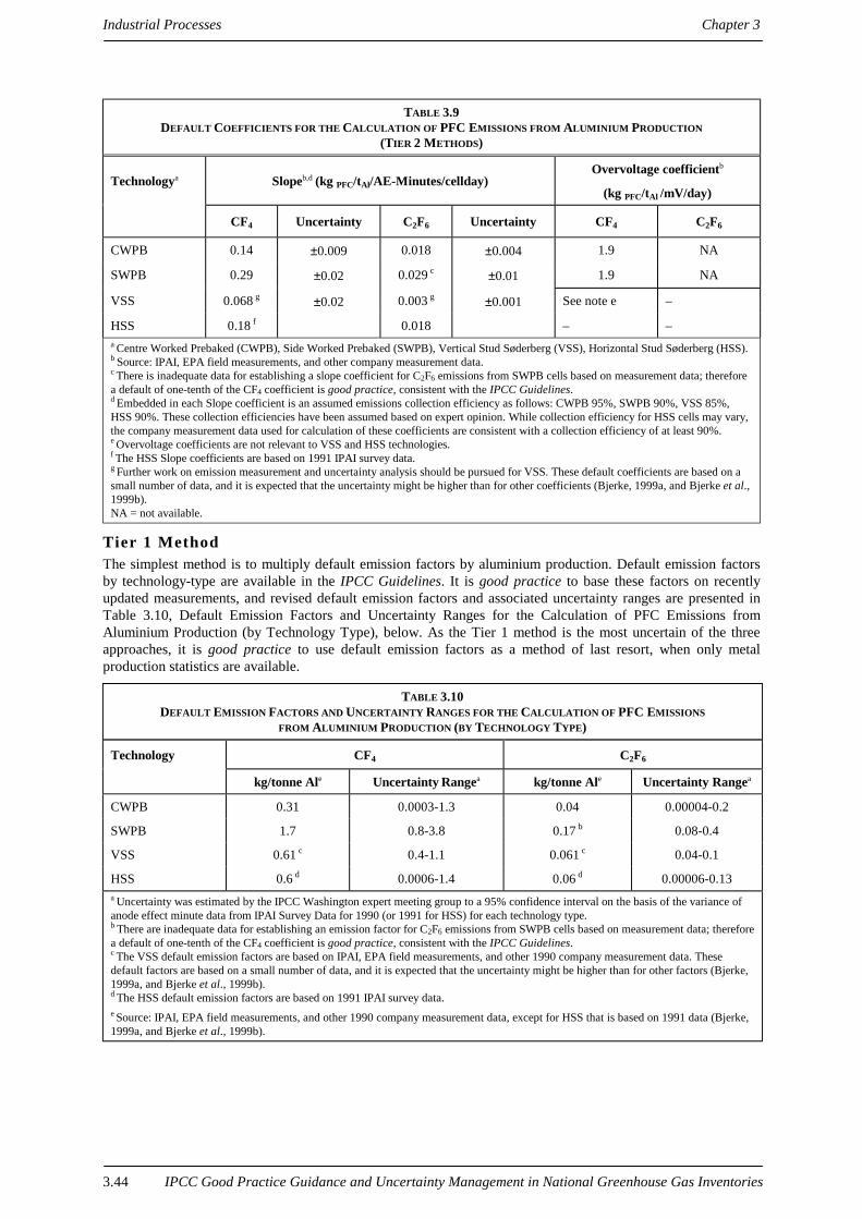
Industrial Processes Chapter 3
IPCC Good Practice Guidance and Uncertainty Management in National Greenhouse Gas Inventories3.44
TABLE 3.9DEFAULT COEFFICIENTS FOR THE CALCULATION OF PFC EMISSIONS FROM ALUMINIUM PRODUCTION
(TIER 2 METHODS)
Technologya Slopeb,d (kg PFC/tAl/AE-Minutes/cellday)Overvoltage coefficientb
(kg PFC/tAl /mV/day)
CF4 Uncertainty C2F6 Uncertainty CF4 C2F6
CWPB 0.14 ±0.009 0.018 ±0.004 1.9 NA
SWPB 0.29 ±0.02 0.029 c ±0.01 1.9 NA
VSS 0.068 g ±0.02 0.003 g ±0.001 See note e –
HSS 0.18 f 0.018 – –a Centre Worked Prebaked (CWPB), Side Worked Prebaked (SWPB), Vertical Stud Søderberg (VSS), Horizontal Stud Søderberg (HSS).b Source: IPAI, EPA field measurements, and other company measurement data.c There is inadequate data for establishing a slope coefficient for C2F6 emissions from SWPB cells based on measurement data; thereforea default of one-tenth of the CF4 coefficient is good practice, consistent with the IPCC Guidelines.d Embedded in each Slope coefficient is an assumed emissions collection efficiency as follows: CWPB 95%, SWPB 90%, VSS 85%,HSS 90%. These collection efficiencies have been assumed based on expert opinion. While collection efficiency for HSS cells may vary,the company measurement data used for calculation of these coefficients are consistent with a collection efficiency of at least 90%.e Overvoltage coefficients are not relevant to VSS and HSS technologies.f The HSS Slope coefficients are based on 1991 IPAI survey data.g Further work on emission measurement and uncertainty analysis should be pursued for VSS. These default coefficients are based on asmall number of data, and it is expected that the uncertainty might be higher than for other coefficients (Bjerke, 1999a, and Bjerke et al.,1999b).NA = not available.
Tier 1 MethodThe simplest method is to multiply default emission factors by aluminium production. Default emission factorsby technology-type are available in the IPCC Guidelines. It is good practice to base these factors on recentlyupdated measurements, and revised default emission factors and associated uncertainty ranges are presented inTable 3.10, Default Emission Factors and Uncertainty Ranges for the Calculation of PFC Emissions fromAluminium Production (by Technology Type), below. As the Tier 1 method is the most uncertain of the threeapproaches, it is good practice to use default emission factors as a method of last resort, when only metalproduction statistics are available.
TABLE 3.10DEFAULT EMISSION FACTORS AND UNCERTAINTY RANGES FOR THE CALCULATION OF PFC EMISSIONS
FROM ALUMINIUM PRODUCTION (BY TECHNOLOGY TYPE)
Technology CF4 C2F6
kg/tonne Ale Uncertainty Rangea kg/tonne Ale Uncertainty Rangea
CWPB 0.31 0.0003-1.3 0.04 0.00004-0.2
SWPB 1.7 0.8-3.8 0.17 b 0.08-0.4
VSS 0.61 c 0.4-1.1 0.061 c 0.04-0.1
HSS 0.6 d 0.0006-1.4 0.06 d 0.00006-0.13a Uncertainty was estimated by the IPCC Washington expert meeting group to a 95% confidence interval on the basis of the variance ofanode effect minute data from IPAI Survey Data for 1990 (or 1991 for HSS) for each technology type.b There are inadequate data for establishing an emission factor for C2F6 emissions from SWPB cells based on measurement data; thereforea default of one-tenth of the CF4 coefficient is good practice, consistent with the IPCC Guidelines.c The VSS default emission factors are based on IPAI, EPA field measurements, and other 1990 company measurement data. Thesedefault factors are based on a small number of data, and it is expected that the uncertainty might be higher than for other factors (Bjerke,1999a, and Bjerke et al., 1999b).d The HSS default emission factors are based on 1991 IPAI survey data.e Source: IPAI, EPA field measurements, and other 1990 company measurement data, except for HSS that is based on 1991 data (Bjerke,1999a, and Bjerke et al., 1999b).

Chapter 3 Industrial Processes
IPCC Good Practice Guidance and Uncertainty Management in National Greenhouse Gas Inventories 3.45
It is good practice to apply the default emission factors that are based on 1990 (or 1991 for HSS) median anodeeffect frequency and duration data, for all years for which there are no process (anode effect) data unless it can bedemonstrated otherwise.
CH O I C E O F A C T I V I T Y D A T AIt is good practice to record the information requested for Tier 3b and Tier 2 methods concerning frequency andduration of anode effects and Anode Effect Overvoltage and production data at the plant level. Individualcompanies or industry groups should be consulted to ensure that the data are available and in a useable format forinventory estimation. For the Tier 1 method, activity data consist of production statistics that should be availablefrom companies at the plant level. Uncertainty in production data (tonnes of aluminium) is likely to be low inmost countries. Given the expected universal availability of production data, production capacity data shouldonly be used as a check on production statistics.
CO M P L E T E N E S SIn principle, production statistics should be available for all smelters. It is good practice to aggregate emissionsestimates from each smelter to estimate total national emissions. All members of the IPAI, who represent 60% of1999 world capacity, report production data. If smelter-level production data are unavailable, smelter capacitydata may be used along with aggregate national production to estimate smelter production. All inventory agenciesshould be able to implement at a minimum level the Tier 1 method and ensure completeness of reporting. Thereis no reason to report the terms NA (not available) and NE (not estimated) for this source category. Whenemissions are being measured by continuous monitoring or for the purposes of calculating emission coefficientsor emission factors, complete coverage of emissions at the smelter level for this source category requiresestimation of emissions of CF4 and C2F6 from the exhaust duct and potroom roof or a good understanding of thecollection efficiency.
DE V E L O P I N G A C O N S I S T E N T T I M E S E R I E SIf all the necessary historical data (e.g. production statistics, AED and AEF or AEO) are available, emissionsover the entire time period can be estimated using the appropriate good practice method.
Where some historical data are missing, it is good practice to use available plant-specific measurements toestablish an acceptable relationship between emissions and activity data in the base year. Implementing anyrelationship retroactively requires that records of process data be available. Most smelters should have records ofprocess data, with perhaps some regional exceptions. In addition to having historical data, each smelter must beable to demonstrate that the relationship to be retroactively implemented is applicable to its historical operatingconditions (i.e. there have been no significant technological or operational changes).20 To ensure consistencyover time, if the estimation method for a smelter changes it is good practice to recalculate emissions estimatesusing both the past and current methodologies to ensure that any trends in emissions are real and not caused bythe change in estimation methodologies. These recalculations should be carried out according to the guidanceprovided in Chapter 7, Methodological Choice and Recalculation, Section 7.3.2.2, Alternative RecalculationTechniques, and all assumptions should be documented clearly.
UN C E R T A I N T Y A S S E S S M E N TIt is possible to apply classical statistical quantitative approaches to estimate uncertainty ranges for the Tier 1,Tier 2 and Tier 3 methods. Tables 3.9, Default Coefficients for the Calculation of PFC Emissions fromAluminium Production (Tier 2 Methods), and 3.10, Default Emission Factors and Uncertainty Ranges for theCalculation of PFC Emissions from Aluminium Production (by Technology Type), provide estimates ofuncertainty associated with emission factors for Tier 1 and Tier 2 methods. The method used to derive thesevalues was a combination of classical statistics (two-sigma estimates) and expert judgement. Uncertainty for theTier 1 method default factors is significantly higher than the Tier 3 and Tier 2 methods because smelter-specificoperating conditions are not reflected in these estimates.
The uncertainty associated with AEF and AED or AEO, when measured, is expected to be low but will dependon computer scan rates (e.g. long scan rates will yield higher uncertainties) and data collection systems at eachsite.
20 If the Tier 3b method is being used, expert judgement should be used to determine when a significant change in operationsor technology at a smelter will require development of a new smelter-specific slope coefficient.
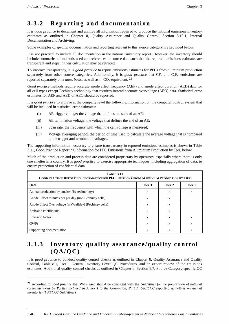
Industrial Processes Chapter 3
IPCC Good Practice Guidance and Uncertainty Management in National Greenhouse Gas Inventories3.46
3 . 3 . 2 R e p o r t i n g a n d d o c u me n t a t i o nIt is good practice to document and archive all information required to produce the national emissions inventoryestimates as outlined in Chapter 8, Quality Assurance and Quality Control, Section 8.10.1, InternalDocumentation and Archiving.
Some examples of specific documentation and reporting relevant to this source category are provided below.
It is not practical to include all documentation in the national inventory report. However, the inventory shouldinclude summaries of methods used and references to source data such that the reported emissions estimates aretransparent and steps in their calculation may be retraced.
To improve transparency, it is good practice to report emissions estimates for PFCs from aluminium productionseparately from other source categories. Additionally, it is good practice that CF4 and C2F6 emissions arereported separately on a mass basis, as well as in CO2-equivalent. 21
Good practice methods require accurate anode effect frequency (AEF) and anode effect duration (AED) data forall cell types except Pechiney technology that requires instead accurate overvoltage (AEO) data. Statistical errorestimates for AEF and AED or AEO should be reported.
It is good practice to archive at the company level the following information on the computer control system thatwill be included in statistical error estimates:
(i) AE trigger voltage; the voltage that defines the start of an AE;
(ii) AE termination voltage; the voltage that defines the end of an AE;
(iii) Scan rate; the frequency with which the cell voltage is measured;
(iv) Voltage averaging period; the period of time used to calculate the average voltage that is comparedto the trigger and termination voltages.
The supporting information necessary to ensure transparency in reported emissions estimates is shown in Table3.11, Good Practice Reporting Information for PFC Emissions from Aluminium Production by Tier, below.
Much of the production and process data are considered proprietary by operators, especially where there is onlyone smelter in a country. It is good practice to exercise appropriate techniques, including aggregation of data, toensure protection of confidential data.
TABLE 3.11GOOD PRACTICE REPORTING INFORMATION FOR PFC EMISSIONS FROM ALUMINIUM PRODUCTION BY TIER
Data Tier 3 Tier 2 Tier 1
Annual production by smelter (by technology) x x x
Anode Effect minutes per pot day (non Pechiney cells) x x
Anode Effect Overvoltage (mV/cellday) (Pechiney cells) x x
Emission coefficients x x
Emission factor x x x
GWPs x x x
Supporting documentation x x x
3 . 3 . 3 I n v e n t o r y q u a l i t y a s s u r a n c e / q u a l i t y c o n t r o l( Q A / Q C )
It is good practice to conduct quality control checks as outlined in Chapter 8, Quality Assurance and QualityControl, Table 8.1, Tier 1 General Inventory Level QC Procedures, and an expert review of the emissionsestimates. Additional quality control checks as outlined in Chapter 8, Section 8.7, Source Category-specific QC
21 According to good practice the GWPs used should be consistent with the Guidelines for the preparation of nationalcommunications by Parties included in Annex I to the Convention, Part I: UNFCCC reporting guidelines on annualinventories (UNFCCC Guidelines).

Chapter 3 Industrial Processes
IPCC Good Practice Guidance and Uncertainty Management in National Greenhouse Gas Inventories 3.47
Procedures (Tier 2), and quality assurance procedures may also be applicable, particularly if higher tier methodsare used to determine emissions from this source category. Inventory agencies are encouraged to use higher tierQA/QC for key source categories as identified in Chapter 7, Methodological Choice and Recalculation.
Additional procedures specific to aluminium production are outlined below:
Comparison of emission factors
Inventory agencies should check if the estimated emission factors are within the range of default emission factorsprovided for the Tier 1 method. If the emission factors are outside of this range, they should assess and documentthe smelter-specific conditions that account for the differences. It may be necessary to repeat measurements forvalidation purposes.
Plant-specif ic data check
The following plant-specific data is required for adequate auditing of emissions estimates:
• Production data;
• Process data records;
• Calculations and estimation method;
• List of assumptions;
• Documentation of sampling, measurement method, and measurement results.
If emission measurements from individual plants are collected, inventory agencies should ensure that themeasurements were made according to recognised national or international standards. QC procedures in use atthe site should be directly referenced and included in the QC plan. If the measurement practices were notconsistent with QC standards, the inventory agency should reconsider the use of these data.
Verif ication of emissions est imates
Global atmospheric measurements of CF4 and C2F6 concentrations can provide an upper limit on the total globalemissions of PFCs from all source categories (Harnisch et al., 1998). This can be used to check emissionsestimates across the international aluminium production source category and potentially to evaluate theconsistency of emission factors and coefficients. While it may be feasible to cross check emissions estimatesfrom this source category by external measurements of plumes from smelters, the procedures for doing this areimpractical, given the current state of technology, and are not required under good practice.

Industrial Processes Chapter 3
IPCC Good Practice Guidance and Uncertainty Management in National Greenhouse Gas Inventories3.48
3 . 4 S F 6 E M I S S I O N S F R O M M A G N E S I U MP R O D U C T I O N
3 . 4 . 1 M e t h o d o l o g i c a l i s s u e s 22
In the magnesium industry, SF6 is used as a cover gas in foundries to prevent oxidation of molten magnesium. Itis assumed that all SF6 used as cover gas is emitted to the atmosphere. It is good practice in inventory preparationin estimating emissions of SF6 from use in the magnesium industry to consider, in a disaggregated way ifpossible, all segments of the industry using SF6. These segments include primary magnesium production, diecasting, gravity casting, and reprocessing (secondary production). It is good practice to assess other magnesiumproduction processes that use and emit SF6.
CH O I C E O F M E T H O DThe choice of a good practice method will depend on national circumstances. The decision tree (see Figure 3.6,Decision Tree for SF6 Emissions from Magnesium Production) describes good practice in adapting the methodsin the IPCC Guidelines (Vol. 3, Section 2.13.8, SF6 Used in Aluminium and Magnesium Foundries) to thesecountry-specific circumstances. The IPCC Guidelines describe a general equation for calculating SF6 emissionsfrom magnesium that is the basis for all the methods described:
EQUATION 3.12Emissions of SF6 = Consumption of SF6 in Magnesium Smelters and Foundries
The most accurate application of this equation requires collecting direct data on SF6 consumption from allindividual users of the gas in the magnesium industry because these figures reflect apparent consumption ratherthan emissions. Consumption is defined as the use of SF6 as a cover gas. In the absence of direct data, it is goodpractice to obtain estimates through a top-down method using production data and emission factors relevant tothe various manufacturing processes. In cases where the data on direct use are incomplete, it is good practice touse a hybrid method that uses direct data where available, and production-based emission factors to complete theestimate. A hybrid approach is preferable to relying solely on the top-down approach.
If no direct data are available, an alternative but a less accurate method is to estimate the share of annual nationalSF6 consumption attributable to the magnesium industry. This requires collecting annual data on national SF6sales and assumes that all SF6 gas sold to the magnesium industry is emitted within the year.
CH O I C E O F E M I S S I O N F A C T O R SSince the direct reporting method assumes that all SF6 consumption is emitted, there is no need to use emissionfactors or coefficients when SF6 consumption data are available. When complete reported data are not available itis good practice to obtain emission factors for each segment of the industry consistent with the decision tree inFigure 3.6, Decision Tree for SF6 Emissions from Magnesium Production. These emission factors should relateSF6 emissions to magnesium production at the same disaggregated level as the available activity data (e.g.national, sub-national). National emission factors based on plant measurements are preferable to internationaldefault factors because they reflect conditions specific to the country. Such information may be accessiblethrough industry associations, surveys or studies.
The IPCC Guidelines do not provide default emission factors for SF6 from magnesium. Under recommendedconditions for die-casting, the consumption rates are about 1 kg SF6 per tonne magnesium produced or smelted(Gjestland, 1996). It is good practice to use this value in the absence of better information. This default value isquite uncertain, however. For example, one diecasting industry survey showed a wide range of SF6 consumptionrates, from 0.1 to 10 kg SF6 per tonne magnesium produced (Palmer, 1999).
22 SF6 is sometimes used in the aluminium industry as a cover gas or for other purposes, and is assumed to be inert. Theemissions of SF6 are therefore assumed to be equal to consumption, and can be estimated using a consumption-basedapproach similar to the consumption-based method for magnesium production. The emission factors and the national salesmethod as discussed for magnesium production are not applicable to SF6 used in aluminium production.

Chapter 3 Industrial Processes
IPCC Good Practice Guidance and Uncertainty Management in National Greenhouse Gas Inventories 3.49
F i g u r e 3 . 6 D e c i s i o n T r e e f o r S F 6 E m i s s i o n s f r o m M a g n e s i u mP r o d u c t i o n
CH O I C E O F A C T I V I T Y D A T AWith the direct-reporting method, the activity data are SF6 consumption totals from each plant. Magnesiumproduction data are necessary for those plants that do not report SF6 consumption data. Where there is somedirect reporting of SF6 use, it is good practice to assess the share of the total segment's magnesium productionthat is represented by the plants that are directly reporting SF6 data. For the other plants, it is good practice to useproduction-based estimates of emissions.
Isthere any
magnesium productionor casting in the
country?
Foreach segments,is SF6 used as a
cover gas?
Report‘Not Occurring’
Estimateemissions using
the national salesmethod
No
Yes
Box 1Yes
Identify segmentsof the magnesium
industry
Continueto the nextsegment
Are therereported data onSF6 use from all
segments?
Estimateemissions using
the directreporting method
Are therereported data onSF6 use from any
segments?
Ismagnesium
production a keysource category?
(Note 1)
Collectplant data
fromcompanies
Arethere activity
level and emissionfactor data?
Estimateemissions
using the top-down method
Estimate emissionsusing the hybrid(direct and top-down) method
Yes Yes
Yes
YesNo
No
No
No No
Box 2
Box 3Box 4
Note 1: A key source category is one that is prioritised within the national inventory system because its estimate has a significantinfluence on a country’s total inventory of direct greenhouse gases in terms of the absolute level of emissions, the trend in emissions, orboth. (See Chapter 7, Methodological Choice and Recalculation, Section 7.2, Determining National Key Source Categories.)
Industrial Processes Chapter 3
IPCC Good Practice Guidance and Uncertainty Management in National Greenhouse Gas Inventories3.50
To the maximum possible extent, it is good practice to disaggregate production data into segments (e.g. primaryproduction, die casting, gravity casting) using SF6 within the magnesium industry to make full use of segment-specific emission factors. Where disaggregated data are not available, more aggregated production data, possiblycombining output from several different processes, may be used to provide an estimate. In the absence of SF6consumption data or magnesium production data, the alternative is to collect annual national data on SF6 sales tothe magnesium industry. This data could come directly from SF6 producers or from national statistics. It is goodpractice to consider data on consumption by other industries that use SF6 (e.g. electrical equipment) whenestimating the share consumed by the magnesium industry.
CO M P L E T E N E S SIncomplete direct reporting or activity data should not be a significant issue for primary production. There is asmall number of primary magnesium producers that are generally well known and keep good records.Completeness issues generally arise in the casting segments, where facilities are more widely distributed, andhave a wide range of capacities and technologies. Some plants may supply to niche markets that are not capturedby national data sets. The inventory agency should confirm the absence of estimates for these smaller industrysegments rather than simply assuming they do not occur. It is also good practice to undertake periodic surveys ofthe industry and establish close links with the local industry associations to check completeness of estimates.
DE V E L O P I N G A C O N S I S T E N T T I M E S E R I E SThere may be issues of data availability associated with establishing historical emissions, particularly whenimplementing a direct reporting approach. It is good practice to use historical SF6 data where available, but SF6purchase records for previous years may not be archived by magnesium manufacturers.
In the absence of such data, a default approach of multiplying activity data by an assumed emission factor may beused. In some cases, emission factors may decrease over time due to environmental awareness, economic factors,and improved technologies and practices. Good practice is to assess the appropriate historical emission factorsfollowing the guidance in Chapter 7, Methodological Choice and Recalculation, Section 7.3.2.2, AlternativeRecalculation Techniques. In some cases, historical production data may not be available due to lack of initialrecords or changes in the structure of the industry in the intervening period. In this case, international productiondata may be used or, if this too is unavailable, a general relationship between national economic activity andmagnesium production. To ensure consistency over time, it is good practice to recalculate emissions estimatesusing previously used and new methods to ensure that any trends in emissions are real and not caused by changesin the estimation methodologies. Good practice is to document assumptions in all cases and archive them at theinventory agency.
UN C E R T A I N T Y A S S E S S M E N TAt the plant level, there is a very low uncertainty associated with plant SF6 use data, since SF6 use is measuredeasily and accurately from purchase data. (An uncertainty estimate of less than 5% is usually appropriate fordirectly reported data.) There is some uncertainty associated with the assumption that 100% of the SF6 used isemitted. Anecdotal evidence suggests that, under certain extreme conditions, a minor portion of SF6 applied mayreact or decompose in the process. For inventory purposes, however, until further peer-reviewed research workclarifies this effect, the assumption is that all SF6 used as a cover gas is emitted. Uncertainties are much higherwhere plant data are not available and emissions could be much higher or lower than indicated by use of theIPCC defaults, as already indicated
At the national inventory level, the accuracy of magnesium production activity data is comparable to that of othernational production statistics (i.e. ±5%). Additional uncertainty is introduced through estimating the share ofproduction not reporting directly. Aggregating production from different segments and using aggregated emissionfactors also introduces uncertainty. For example, national data from casting operations may not be segregatedinto die-casting and gravity casting segments despite their potentially different SF6 emission rates. Estimating SF6emissions on the basis of sales to the magnesium industry each year is highly uncertain, because SF6 may bepurchased in bulk quantities and not used until later years. The uncertainty in this case will be bounded by thetotal sales data.
3 . 4 . 2 R e p o r t i n g a n d d o c u me n t a t i o nIt is good practice to document and archive all information required to produce the national emissions inventoryestimates as outlined in Chapter 8, Quality Assurance and Quality Control, Section 8.10.1, Internal

Chapter 3 Industrial Processes
IPCC Good Practice Guidance and Uncertainty Management in National Greenhouse Gas Inventories 3.51
Documentation and Archiving. It is not practical to include all documentation in the national inventory report.However, the inventory should include summaries of methods used and references to source data such that thereported emissions estimates are transparent and steps in their calculation may be retraced.
To improve transparency, it is good practice to report emissions estimates from this source category separatelyby industry segment.
The following additional information can provide a reasonable degree of transparency in reporting:
Direct Reporting
• Number of plants reporting;
• Magnesium and magnesium products production;
• SF6 emissions;
• Emission factor data (and reference).
National SF6 sales-based estimate of potential emissions
• National SF6 consumption (and reference);
• Assumptions for allocating SF6 used to magnesium;
• Estimate of percentage of national SF6 used in magnesium (and reference);
• Any other assumptions made.
In most countries, the magnesium industry will be represented by a small number of plants. In this industry, theactivity level data and SF6 emissions (that are directly related to activity levels) may be considered confidentialbusiness information and public reporting may be subject to confidentiality considerations.
3 . 4 . 3 I n v e n t o r y q u a l i t y a s s u r a n c e / q u a l i t y c o n t r o l( Q A / Q C )
It is good practice to conduct quality control checks as outlined in Chapter 8, Quality Assurance and QualityControl, Table 8.1 Tier 1 General Inventory Level QC Procedures, and an expert review of the emissionsestimates. Additional quality control checks, as outlined in Chapter 8.7, Source Category-specific QC Procedures(Tier 2), and quality assurance procedures may also be applicable, particularly if higher tier methods are used todetermine emissions from this source category. Inventory agencies are encouraged to use higher tier QA/QC forkey source categories as identified in Chapter 7, Methodological Choice and Recalculation.
Additional procedures specific to magnesium production are outlined below:
Comparison of emissions est imates using different approaches
If emissions were calculated using data from individual plants (bottom-up approach), inventory agencies shouldcompare the estimate to emissions calculated using national magnesium production data or national SF6consumption (top-down approach). The results of the comparison should be recorded and any discrepanciesshould be investigated.
Review of plant- level data
The following plant-specific information should be archived to facilitate independent review:
• SF6 consumption or magnesium production (where factors are used);
• Plant-level QA/QC results (including documentation of sampling, measurement method, and measurementresults for plant level data);
• Results of QA/QC conducted by any integrating body (e.g. industry association);
• Calculations and estimation method;
• Where applicable, a list of assumptions in allocating national SF6 usage or production to plant level.
Inventory agencies should determine if national or international measurement standards were used for SF6consumption or magnesium production data at the individual plants. If standard methods and QA/QC were notfollowed, then they should reconsider the use of these activity data.

Industrial Processes Chapter 3
IPCC Good Practice Guidance and Uncertainty Management in National Greenhouse Gas Inventories3.52
Review of national act ivity data
QA/QC activities associated with the reference to magnesium production data should be evaluated andreferenced. Inventory agencies should check if the trade association or agency that compiled the nationalproduction data used acceptable QA/QC procedures. If the QA/QC procedures are deemed acceptable, inventoryagencies should reference the QC activity as part of the QA/QC documentation.
Assessment of emission factors
Where country-specific SF6 factors are used, inventory agencies should review the level of QC associated withthe underlying data. Although there is no IPCC default emission factor, good practice is that the inventoryagency cross-check national level default factors against plant-level factors to determine their representativeness.
Peer review
Inventory agencies should involve magnesium industry experts in a thorough review of the inventory estimate,giving consideration to potential confidentiality issues. Historical production data may be less sensitive to publicdisclosure than current data and could be utilised for an external peer review of plant level emissions.
Verif ication of SF6 emissions data
Inventory agencies should sum the amount of SF6 used by different industrial sectors (e.g. magnesium, electricalequipment) and compare this value with the total usage of SF6 in the country, obtained from import/export andproduction data. This provides an upper bound on the potential emissions.23
23 It may not always be the case that such aggregated consumption data will provide an upper limit on emissions. It ispossible, depending on the national characteristics of the SF6 consuming industry that in some years actual emissions of SF6may be greater than consumption of SF6. For instance, consumption in die casting of magnesium may be very low, there maynot be much semiconductor manufacturing, but a considerable bank of SF6 in electrical equipment may have evolved throughthe years. In this case, leakage from bank combined with emissions resulting from decommissioning of equipment may leadto actual emissions that exceed consumption of SF6 (potential emissions). See also Table 3.12, Default Emission Factors forSF6 Emissions from Electrical Equipment – Tier 2 (fraction of SF6/yr).

Chapter 3 Industrial Processes
IPCC Good Practice Guidance and Uncertainty Management in National Greenhouse Gas Inventories 3.53
3 . 5 E M I S S I O N S O F S F 6 F R OM E L E C T R I C A LE Q U I P M E N T A N D O T H E R S O U R C E S
3 . 5 . 1 E l e c t r i c a l e q u i p me n t
3.5.1.1 Methodological issuesSulfur hexafluoride (SF6) is used for electrical insulation, arc quenching, and current interruption in equipmentused in the transmission and distribution of electricity. Most of the SF6 used in electrical equipment is used in gasinsulated switchgear (GIS) and circuit breakers, though some SF6 is used in high voltage gas-insulatedtransmission lines and other equipment. SF6 emissions from electrical equipment are the largest global sourcecategory of SF6 emissions.
CH O I C E O F M E T H O DThe choice of good practice method will depend on national circumstances. The decision tree, Figure 3.7,Decision Tree for SF6 from Electrical Equipment, describes good practice in adapting the methods in the IPCCGuidelines to these country-specific circumstances.
The IPCC Guidelines include methods for estimating both potential (Tier 1 method) and actual (Tier 2 method)emissions of SF6 from electrical equipment. This section describes good practice for using the Tier 1 method andtwo variants of the current Tier 2 method. Three variants of a more accurate approach (termed Tier 3 method) arealso described. Emissions estimates developed using the Tier 3 method will be the most accurate. Estimatesdeveloped using the Tier 1 method will be the least accurate because these figures reflect apparent consumptionrather than emissions.
Tier 3 Method – Mass-balance approachThe Tier 3 method is the most accurate approach for estimating actual emissions of SF6 from electricalequipment. It is a mass-balance approach that tracks the amount of new SF6 introduced into the industry eachyear. Industry uses some of this newly purchased SF6 to replace leaked gas that escaped to the atmosphere theprevious year. The remainder of the new SF6 is used to fill an increase in total equipment capacity, and thus doesnot replace leaked gas. To develop an accurate estimate, therefore, this approach distinguishes between the SF6
used to replace emitted gas and SF6 used to increase total equipment capacity or replace destroyed gas.24
The main advantages of this approach are: (i) equipment manufacturers and facilities can readily track therequired information, and (ii) it does not depend on global default emissions factors that are subject toconsiderable uncertainty. This tier can be implemented at different levels of aggregation depending on data andresource availability. The most accurate approach is to estimate emissions from each lifecycle stage of theequipment at the facility level (Tier 3a method). Alternatively, the life cycle calculation may be bypassed andemissions can be estimated at the aggregate facility level (Tier 3b method) or at the country level (Tier 3cmethod). Inventory agencies are encouraged to use the most detailed approach that is practical, and to usealternative estimation methods to check the results.
24 For example, suppose that 100 circuit breakers are retired in a country in a certain year, and 150 new circuit breakers (withthe same average charge size as the retiring breakers) are installed. In this case, the manufacturers or users of the circuitbreakers in that country must purchase at least enough gas to charge 50 circuit breakers, even if they recover all of the gasfrom the retiring 100 circuit breakers and use it to fill 100 of the breakers that replace them. The gas used to charge the 50‘extra’ circuit breakers is used to fill an increase in equipment capacity, and does not replace emitted gas. Some gas that iscontaminated during inspection is destroyed using thermal destruction methods.

Industrial Processes Chapter 3
IPCC Good Practice Guidance and Uncertainty Management in National Greenhouse Gas Inventories3.54
F i g u r e 3 . 7 D e c i s i o n T r e e f o r S F 6 f r o m E l e c t r i c a l E q u i p m e n t
IsSF6 used inelectrical
equipment?
Are SF6 survey dataavailable from
facilities?
Report‘Not Occurring’
No
Yes
Areactivity data and
emission factors availablefor the Tier 2a
approach?
Aredata available
for the charges ofinstalled and retiring
equipment?
Canan annual
survey of facilitiesthat use SF6 be
completed?
Estimate emissionsusing Tier 1
‘Potential Emissions’approach
No
Box 1
Is thisa key source
category?(Note 1)
Are SF6 survey dataavailable by life
cycle stage?
Estimate emissionsusing Tier 3b
‘Manufacturer-Utility’ approach
Box 5
Estimate emissionsusing Tier 2b IPCC‘Emission Factor’
approach
Box 2Estimate emissionsusing Tier 2b ‘Life-Cycle Emissions’
approach
Box 3
Estimate emissionsusing Tier 3a‘Life-Cycle’
approach
Box 4
Estimate emissionsusing Tier 3c
‘Country Mass-Balance’ approach
Box 6
Conduct survey offacilities that use SF6.Determine if life cycle
data are needed.
No
Yes
No
Yes NoYes
No
Yes
No
Yes
Yes
Note 1: A key source category is one that is prioritised within the national inventory system because its estimate has a significantinfluence on a country’s total inventory of direct greenhouse gases in terms of the absolute level of emissions, the trend in emissions, orboth. (See Chapter 7, Methodological Choice and Recalculation, Section 7.2, Determining National Key Source Categories.)

Chapter 3 Industrial Processes
IPCC Good Practice Guidance and Uncertainty Management in National Greenhouse Gas Inventories 3.55
Tier 3a Method – Emissions by life cycle stage of equipmentThis approach is useful for inventory agencies or facilities that, in addition to estimating their total emissions ofSF6 from electrical equipment, wish to determine how and when such emissions occur during the lifecycle of theequipment. Information on how and when emissions occur is important for focusing mitigation efforts where theywill be most effective. The method includes separate equations for each phase of the lifecycle of equipment,including equipment manufacture, installation, usage, and disposal. Ideally, data are obtained for everyequipment manufacturer and utility in the country, and the emissions of all manufacturers and utilities aresummed to develop the national estimate. The basic equation is:
EQUATION 3.13
Total Emissions = Σ Manufacturing Emissions + Σ Installation Emissions
+ Σ Use Emissions + Σ Disposal Emissions
In the above equation, national emissions for each phase are equal to the sum of all equipment manufacturers’emissions for each phase.
Each equipment manufacturer’s emissions can be calculated in three steps:
(i) Collect the data on the net decrease in their annual SF6 inventory on hand. (Note that if theinventory increases, this will be a negative number);
(ii) Add the amount of SF6 obtained during the year (including any SF6 purchased from producers ordistributors, any SF6 returned from equipment users, and any SF6 returned by users after recycling);
(iii) Subtract the amount of SF6 transferred to others during the year (including the amount of SF6 innew equipment delivered to customers, the amount delivered to equipment users in containers, andthe amount returned to SF6 producers, sent to recycling firms, or destroyed).
Equipment installation emissions can be estimated by subtracting the nameplate capacity25 of all new equipmentfilled from the actual amount of SF6 used to fill new equipment.
Equipment use emissions are determined by the amount of SF6 used to service equipment. If SF6 is beingrecovered from equipment before servicing and returned after servicing, it is important that this amount not beincluded in the estimate.
Emissions from equipment disposal are estimated by subtracting the amount of SF6 recovered from retiredequipment from the nameplate capacity of the retired equipment and also subtracting the amount of SF6destroyed.
Tier 3b Method – Manufacturer and util ity-level mass-balance methodIf data for estimating emissions from lifecycle stages are unavailable, emissions can be estimated by trackingoverall consumption and disposal of SF6 for all utilities and manufacturers. Beginning with the equation for Tier3a method, installation, use, and disposal emissions are aggregated into the category of utility emissions. Theequation presented in Tier 3a method is thus simplified to:
EQUATION 3.14
Total Emissions = Σ Manufacturer Emissions + Σ Utility Emissions
Using this approach, equipment manufacturer emissions are estimated as for the Tier 3a method.
Utility emissions are equal to the sum of emissions from all utilities. Each utility’s emissions can be calculatedthrough the following seven steps:
25 Nameplate capacity – The ‘nameplate capacity’ is the quantity of SF6 required to fill a piece of equipment so that it willfunction properly. It may also be referred to as the ‘charge’ and is generally indicated by the nameplate of the equipment. The‘total nameplate capacity’ of all the equipment in a country or facility is the sum of the proper, full charges of all theequipment in use in that country or facility.

Industrial Processes Chapter 3
IPCC Good Practice Guidance and Uncertainty Management in National Greenhouse Gas Inventories3.56
(i) Determine the net decrease in the amount of SF6 stored in containers over the reporting year;
(ii) Add the amount of SF6 purchased from producers/distributors and equipment manufacturers,including the amount of SF6 contained in purchased equipment;
(iii) Subtract the amount of SF6 returned to suppliers;
(iv) Add SF6 returned after recycling;
(v) Subtract any SF6 sent to recycling firms, sold to other entities, or destroyed by the utility orinstallation;
(vi) Add the nameplate capacity of retired equipment;
(vii) Subtract the nameplate capacity of new equipment.
Tier 3c Method – Country-level mass-balance methodIn some cases, it may be impractical for inventory agencies to obtain emissions data from all equipmentmanufacturers and utilities, or such data may be incomplete. In this case, a national level estimate can bedeveloped based on annual national sales of SF6 into the electrical sector (current and historical), equipmentimports and exports, SF6 destruction, and, if possible, country-specific equipment lifetime assumptions. The basicequation is:
EQUATION 3.15Emissions = Annual Sales – (Net Increase in Nameplate Capacity) – (SF6 Destroyed)
Annual sales are equal to new SF6 for filling or refilling electrical equipment, both in bulk and in equipmentitself.
Net increase in nameplate capacity can be calculated through the following steps:
(i) Collect data on the nameplate capacity of new equipment, including both equipment that is filled inthe factory before shipment and equipment that is filled after installation;
(ii) Subtract the nameplate capacity of all retiring equipment.
It is good practice to include the quantity of SF6 destroyed from all electrical equipment in SF6 destroyed.
Tier 2a Method – Life-cycle emission factor approachIf only limited data are available on annual sales of SF6 to equipment manufacturers and utilities, emissions canbe estimated for each stage of the lifecycle of the equipment, using emission factors that are unique to each stage.Good practice is to use the following equation:
EQUATION 3.16Total Emissions = Manufacturing Emissions + Installation Emissions
+ Use Emissions + Disposal Emissions
Manufacturing emissions are estimated by using emission factors based on the amount of SF6 purchased byequipment manufacturers, or the nameplate capacity of new equipment charged.
Similarly, equipment installation emissions are estimated using either purchase-based or nameplate-basedemission factors. This will require data on either the amount of SF6 purchased by utilities for new equipment orthe nameplate capacity of new equipment charged by utilities (not equipment manufacturers). In some cases, thenameplate capacity of new equipment may be known, but not the fractions of this capacity filled bymanufacturers versus utilities. Under these circumstances, a single ‘Manufacturing/Installation Emission Factor’can be multiplied by the total nameplate capacity of new equipment.
Equipment use emissions are estimated by multiplying the total nameplate capacity of installed equipment by a‘Use Emission Factor’. The ‘use emission factor’ includes emissions due to leakage, and servicing andmaintenance that are typically carried out every 12 years.
Finally, equipment disposal emissions are estimated by multiplying the nameplate capacity of retiring equipmentby the assumed fraction of SF6 left in equipment at the end of its life. If SF6 is being recovered, good practice is

Chapter 3 Industrial Processes
IPCC Good Practice Guidance and Uncertainty Management in National Greenhouse Gas Inventories 3.57
to adjust the resulting estimate to reflect recovery, by multiplying by (1 – the recovery factor). The defaultrecovery factor is zero. Other factors should be country-specific and determined at the site-level.
Tier 2b Method – IPCC default emission factorsIf inventory agencies only have information on the total charges of installed and retiring equipment, the emissionfactors can be applied at a national level, as described in the IPCC Guidelines:
EQUATION 3.17Emissions of SF6 in year t = (2% of the Total Charge of SF6 Contained in the Existing Stock of
Equipment of Operation in year t) + (95% of the Nameplate Capacity of SF6 in RetiringEquipment)
The first term of the equation estimates leakage and maintenance losses as a fixed percentage of the total charge(e.g. 2%). The existing stock of equipment in each year includes all equipment installed in that year in addition topreviously installed equipment that is still in use. The second term calculates emissions from retiring equipment(e.g. after a lifetime of 30 years) and assumes that the minimum charge is 90%. Recent experience indicates thatthe default assumption of 70% in the IPCC Guidelines underestimates retiring emissions, because equipmentdoes not function below 90% capacity and will be refilled during its lifetime (Bitsch, 1999b). Thus, inventoryagencies using this approach are encouraged to review the applicability of the emissions factors in the equationand use country-specific emission factors if appropriate – especially with respect to implemented recyclingprocedures.
Tier 1 Method – Potential approachThe simplest estimation method in the IPCC Guidelines estimates potential emissions of SF6 from all uses byequating emissions to total consumption of SF6:
EQUATION 3.18Potential SF6 Emission = Production + (Imports – Exports) – Destruction
Inventory agencies will need to determine how much of the total SF6 is sold to utilities and equipmentmanufacturers. This can be done directly (by obtaining data on such sales) or indirectly (by obtaining data onsales for other uses). The direct approach uses the following equation:
EQUATION 3.19SF6 Emissions from Electrical Equipment = Sales of SF6 to Equipment Manufacturers + Sales of
SF6 to Utilities + (SF6 in Imported Equipment – SF6 in Exported Equipment)
The indirect approach is as follows:
EQUATION 3.20SF6 Emissions = Production + (Imports – Exports) – Destruction – Consumption by Other SF6 Uses (i.e. Mg Smelting,
Semiconductor Manufacturing, Other Uses)
Both equations implicitly assume that all SF6 sold into the electrical sector replaces released gas, when in factsome of that SF6 may be used to fill a net increase in the nameplate capacity of installed equipment or to replacedestroyed gas. Good practice considers estimates developed using the Tier 1 method an upper bound.
CH O I C E O F E M I S S I O N F A C T O R SAs of the variability of emissions rates from region to region, inventory agencies using the Tier 2 method areencouraged to develop and use their own emissions factors. Surveying a representative sample of equipmentmanufacturers and utilities within the country is an effective way to develop such factors.

Industrial Processes Chapter 3
IPCC Good Practice Guidance and Uncertainty Management in National Greenhouse Gas Inventories3.58
Tier 2a MethodEmission factors for the Tier 2a method are developed based on data collected from representative manufacturersand utilities that track emissions by life cycle stage, essentially using the Tier 3a method at their facilities for oneyear. Total emissions from the survey of manufacturers are summed and then divided by the surveyed facilities’new equipment capacity. This emission factor can then be applied to the manufacturing sector as a whole, usingnational new equipment capacity.
Tier 2b MethodFor developing emission factors for the Tier 2b method, it is good practice for surveyed utilities to track theirtotal consumption of SF6 for refilling of equipment, the total nameplate capacity of their equipment, the quantityof SF6 recovered from retiring equipment, and the nameplate capacity of their retiring equipment. It is goodpractice to sum emissions from the servicing and disposal of equipment across surveyed utilities. The resultingtotal emissions estimates for servicing and disposal are then divided by the surveyed utilities’ total installedequipment capacity or by their total retiring equipment capacity, respectively, to calculate emission factors foruse and for disposal.
The IPCC Guidelines do not provide default emission factors for each lifecycle stage, but suggested factors havebeen developed for some regions based on recent research. These factors are shown in Table 3.12, DefaultEmission Factors for SF6 Emissions from Electrical Equipment – Tier 2 (fraction of SF6/yr).
TABLE 3.12DEFAULT EMISSION FACTORS FOR SF6 EMISSIONS FROM ELECTRICAL EQUIPMENT – TIER 2 (FRACTION OF SF6/YR)
Phase Manufacturing Installation Use Retired Equipment
Region before1996
Since1996
before1996
Since1996
before1996
Since 1996 Lifetime Remaining Recovery
Europeb 0.15 0.06 NA 0.06 NA NA NA NA NA
Japana 0.3 0.3 NA NA 0.001 0.001 NA NA NA
Globalc NA NA 0.15 0.15 0.05 0.02 30 years 0.95 NAa Emission factors of use phase are only for natural emissions (Denki Kyodo Kenkyu, 1998 and Chemical Products Council, 1999).Sources:b Bitsch, 1999a.c Olivier and Bakker, 2000.NA = not available.
CH O I C E O F A C T I V I T Y D A T AThe guidance given below for the Tier 3 methods applies to the same parameters when they are used in the Tier 2and Tier 1 methods. The only unique requirement for the Tier 2 method is the total nameplate capacity ofequipment. Nameplate capacity may be estimated either by surveying utilities directly, or by surveying equipmentmanufacturers regarding their sales of equipment over the lifetime of the equipment (e.g. for the last 30 years).
Tier 3a Method – Emissions by life cycle stageSince Tier 3a method does not rely on emissions factors, the quality of the estimate depends on the accuracy andcompleteness of surveyed activity data. The data should be available directly from individual manufacturers, orthrough manufacturer associations.
Equipment manufacturing: A complete survey of all equipment manufacturers includes, at a minimum, data onthe movement of SF6 through the production and assembly phase, and data on handling emissions of the gas afterdelivery to manufacturing sites. The survey should request enough information to provide a full accounting ofSF6 consumption and losses during the production phase. Annual mass balance tables can be used to estimatehow much SF6 gas is lost due to emission releases and what fraction this is of nominal SF6 content of totalelectrical equipment produced.
If survey data are not available for all manufacturers, alternative methods can be considered (e.g. based onextrapolation of production capacity). Good practice is to use survey data as far as possible and only supplementthem with extrapolative approaches where survey data is not available. For guidance on extrapolating when dataare not available, see Chapter 7, Methodological Choice and Recalculation, Section 7.3.2.2, AlternativeRecalculation Techniques.

Chapter 3 Industrial Processes
IPCC Good Practice Guidance and Uncertainty Management in National Greenhouse Gas Inventories 3.59
Equipment installation: All utilities and other users of electrical equipment should track and record thenameplate capacity of the equipment that is filled. Utilities should also track the amount of SF6 that is used to fillequipment by weighing cylinders before and after filling operations, and tracking any SF6 that is already in theshipped equipment (e.g. to maintain a slight positive pressure during shipment). If filling is performed by theequipment manufacturer rather than by the utility, then the manufacturer may provide this information to theutility.26 Where there are gaps and omissions in the survey, it is possible to use estimates of SF6 stock additionsand default emission rates for installation and set-up procedures.
Equipment use: It is good practice to calculate the quantity of SF6 used to refill equipment by weighingcylinders before and after filling operations.
Equipment disposal: The quantity of SF6 recovered from equipment may be calculated by weighingrecovery cylinders before and after recovery operations. Data on disposal should include all equipment, includingimported equipment.
Tier 3b Method – Manufacturer and util ity-level mass-balance methodEquipment manufacturers: Same as for Tier 3a, above.
Util i t ies: To collect the information necessary to use the Tier 3b method, a survey of all utilities is required.Good practice is to survey industrial sites, military installations, and other non-utility sites that use significantamounts of SF6 in electrical equipment. Some, but not all, of the above information may also be obtained fromequipment manufacturers.
If the utility does not perform all of its own installation, maintenance, and disposal of equipment, persons whoprovide these services should provide data to the utility (e.g. the quantity of gas used to refill equipment, if thisgas did not come from the utility’s own inventory). A full accounting of SF6 emissions associated with handlingand filling losses needs to be collected. This accounting can be based on annual mass balance tables that includethe amount of SF6 already contained in the equipment when shipped to the site. The party responsible for trackingSF6 handling and filling operations needs to be identified, since this can vary from site to site.
Tier 3c Method – Country-level mass-balance methodAnnual sales: Chemical manufacturers or importers or both should be able to supply the most complete data.If information from chemical manufacturers is not available, it is good practice to contact both equipmentmanufacturers and utilities to ensure complete data on SF6 used to fill both new and existing equipment.
Nameplate capacity of new and ret iring equipment: Nameplate capacity can be estimated using oneof the following data sources: (1) information from equipment manufacturers/importers on the total nameplatecapacity of the equipment they manufacture or import and export, (2) information from utilities on the totalnameplate capacity of the equipment they purchase and install each year, or (3) information from chemicalmanufacturers/importers on their sales of SF6 to equipment manufacturers. The first two data sources arepreferable to the third, because gas sales to new equipment manufacturers will differ to some extent from thenameplate capacity of new equipment. In estimating the nameplate capacities of new and retiring equipment,inventory agencies should include the nameplate capacity of imported equipment and exclude the nameplatecapacity of exported equipment. (See Section 3.7.4, Stationary Refrigeration Sub-source Category, Box 3.4,Accounting for Imports and Exports of Refrigerant and Equipment, for a full discussion of how to treat importsand exports in estimating these quantities.)
In the case of retiring equipment, capacity or sales information should be historical, starting in the year when thecurrent year’s retiring equipment was built. The default value for the lifetime of electrical equipment is 30 years.If information on the total nameplate capacity of retiring equipment is not available, it can be estimated from newnameplate capacity, using the estimated annual growth rate of equipment capacity. In estimating the growth rate,
26 The quantity already in shipped equipment may be calculated by multiplying the internal volume of the equipment by thedensity of SF6 at the shipment pressure, or by multiplying the nameplate capacity of the equipment by the ratio of theshipping pressure to the nameplate pressure, in absolute terms (e.g. Pa or psi). In theory, equipment that arrives at the utilityalready completely filled does not need to be included in this calculation, because the quantity of SF6 inside the equipmentwill be identical to the nameplate capacity, and the two will simply cancel. However, utilities are encouraged to track thetotal nameplate capacity of the equipment they install, because this quantity is useful for calculating emissions using the Tier3 and Tier 2 methods and for understanding emissions during equipment use.

Industrial Processes Chapter 3
IPCC Good Practice Guidance and Uncertainty Management in National Greenhouse Gas Inventories3.60
it is good practice to consider both the number of pieces of equipment sold each year and the average nameplatecapacity of the equipment.27
The following equation can be used to estimate retiring nameplate capacity, if this information is not availabledirectly:
EQUATION 3.21Retiring Nameplate Capacity = New Nameplate Capacity / ( 1 + g )L
Where:
L = equipment lifetime
g = rate of growth
According to a 1997 survey, the average annual growth rate of SF6 sales to equipment manufacturers between1991 and 1996 was 6.7%, while the average rate of growth between 1986 and 1996 was 5.3% (Science andPolicy Associates, 1997). In the absence of country-specific information, it is good practice to use a defaultfactor of 6%.
Quantity destroyed: The amount of SF6 destroyed can be estimated using information from electrical equipmentmanufacturers, utilities, chemical manufacturers, or destruction facilities. It is necessary to ensure that thequantities of SF6 reported as destroyed do not include quantities from sources other than electrical equipment.
CO M P L E T E N E S SCompleteness for this source category requires accounting for emissions both at utility facilities and during themanufacture of electrical equipment. Where Tier 3 methods are used, completeness requires that all SF6 users(manufacturers and utilities) be identified.
In the manufacturing sector, this requires assessing emissions from:
• GIS and circuit breaker manufacturers;
• Manufacturers of high voltage gas-insulated transmission lines, substations (mini-stations) and transformers;
• Minor SF6 users, including medium voltage equipment manufacturers and equipment remake manufacturers;
• SF6 moving from producers and distributors to manufacturing facilities.
In the utility sector, this requires accounting for all SF6 losses associated with:
• New electrical equipment installations;
• Leakage, refill and maintenance;
• Disposal of discarded electrical equipment.
It is good practice to identify and include industrial, military and small-utility applications if these are believed tocontribute substantially to total emissions from this source category.
DE V E L O P I N G A C O N S I S T E N T T I M E S E R I E SWhen estimating emissions over a time series, it is necessary to consider SF6 emissions associated withmanufacturing and all installed equipment at utilities for the years of interest. Developing an accurate historicalestimate for installed equipment thus requires information on the capacity and performance of equipmentinstalled for 20 to 30 years preceding the years of interest.
On the manufacturing side, if historical data for developing base year emissions for 1990/1995 are not available,the top-down method calibrated to more accurate account balances for current years may be applied. Since SF6handling practices of equipment manufacturers may have changed substantially since 1995 (e.g. more gas isrecovered), it is not good practice to apply current loss rates to historical estimates. Aggregate loss ratesdetermined from global and regional sales and emission analyses may assist in providing an unbiased estimate forearlier years. It is good practice to recalculate emissions according to the guidance provided in Chapter 7,
27 While the number of pieces of equipment sold each year has generally grown, the average nameplate capacity hasgenerally declined.

Chapter 3 Industrial Processes
IPCC Good Practice Guidance and Uncertainty Management in National Greenhouse Gas Inventories 3.61
Methodological Choice and Recalculation, Section 7.3.2.2, Alternative Recalculation Techniques, with allassumptions clearly documented.
In the utility sector, if historical data for the period 1970-1995 are unavailable, good practice is to developestimates using the top-down method, and then calibrate as discussed above. Average leakage rates for newequipment, and the frequency of refill and routine maintenance all decreased from 1970 to 1995.28 It is goodpractice not to apply current (post-1995) overall loss rates to historical years. Aggregate loss rates can be used inthis case as well.
UN C E R T A I N T Y A S S E S M E N TWhen using Tier 3 methods, the resulting emissions estimates are likely to be more accurate than Tier 2 or Tier 1methods, of the order of ±10%. If surveys are incomplete or only top-down consumption data are available, theassociated uncertainty will be greater. Particular sources of uncertainty in the Tier 3 methods estimates mayinclude:
• SF6 exported by equipment manufacturers (either in equipment or separately in containers);
• SF6 imported by foreign equipment manufacturers (either in equipment or in containers);
• SF6 returned to foreign recycling facilities;
• Time lag between emissions and servicing;29
• Lifetime of the equipment.
The uncertainties in the default emission factors recommended for the Tier 2 method are shown in Table 3.13,Uncertainties for Default Emission Factors for SF6 Emissions from Electrical Equipment. As the Tier 1 methodestimates potential rather than actual emissions, Tier 1 estimates will have an uncertainty of the order of 100% ormore in representing an estimate of actual emissions.
TABLE 3.13UNCERTAINTIES FOR DEFAULT EMISSION FACTORS FOR SF6 EMISSIONS FROM ELECTRICAL EQUIPMENT
Phase Manufacturing Installation Use Retired Equipment
Region <1996 1996- <1996 1996- <1996 1996- Lifetime Remaining Recovery
Europe ±30% ±30% NA ±30% NA NA NA NA NA
Japan ±30% ±30% NA NA NA NA NA NA NA
Global Larger Larger ±30% ±30% ±40% ±50% ±30% ±5% NA
NA= not available.
Source: Olivier and Bakker (2000).
3.5.1.2 Reporting and documentationIt is good practice to document and archive all information required to produce the national emissions inventoryestimates as outlined in Chapter 8, Quality Assurance and Quality Control, Section 8.10.1, InternalDocumentation and Archiving. It is not practical to include all documentation in the national inventory report.However, the inventory should include summaries of methods used and references to source data such that thereported emissions estimates are transparent and steps in their calculation may be retraced.
28 Standards for leakage from GIS are now 1%, but were as much as 3% prior to 1980. In addition, maintenance intervalshave increased, from 3-5 years to 8 years for circuit breakers and about 12 years for GIS.
29 The sales-based method is designed to yield a good estimate of the quantity of chemicals used to replace emittedchemicals in a given year. However, because some equipment may leak but nevertheless continue to run with less than a fullcharge, emitted chemicals are not always replaced during the year that it leaks. Thus, under some circumstances, the sales-based method may slightly either over or underestimate actual emissions. (The net effect of the time lag is to make emissionsappear to occur later in the life of equipment than they actually do.) The frequency of servicing and the growth rate of theequipment stock should be investigated to ascertain the size of any error.

Industrial Processes Chapter 3
IPCC Good Practice Guidance and Uncertainty Management in National Greenhouse Gas Inventories3.62
Some examples of specific documentation and reporting relevant to this source category ensuring transparency inreported emissions estimates are provided in Table 3.14, Good Practice Reporting Information for SF6 Emissionsfrom Electrical Equipment by Tier.
Confidentiality issues may arise where there are limited numbers of manufacturers or utilities. In these cases,aggregated reporting for the total electrical equipment sector, or even total national SF6 applications, may benecessary. If survey responses cannot be released as public information, third party review of survey data may benecessary to support data verification efforts.
TABLE 3.14GOOD PRACTICE REPORTING INFORMATION FOR SF6 EMISSIONS FROM ELECTRICAL EQUIPMENT BY TIER
Data Tier 3a Tier 3b Tier 3c Tier 2a Tier 2b Tier 1
Annual sales of SF6 to equipment manufacturersand utilities X X
Nameplate capacity of new equipment X X X X
Nameplate capacity of existing equipment X X
Nameplate capacity of retiring equipment X X X X X
SF6 destroyed X X X X
SF6 in inventory at beginning of year X X
SF6 in inventory at end of year X X
SF6 purchased by facility X X
SF6 sold or returned by facility X X
SF6 sent off-site for recycling X X
SF6 returned to site after recycling X X
SF6 used to fill new equipment X
SF6 used to service equipment X
SF6 recovered from retiring equipment X
Emission/recovery factors X X
Documentation for factors, if country-specific X X
Production of SF6 X
Consumption of SF6 by other uses X
Imports of SF6 X
Exports of SF6 X
3.5.1.3 Inventory quality assurance/quality control (QA/QC)It is good practice to conduct quality control checks as outlined in Chapter 8, Quality Assurance and QualityControl, Table 8.1, Tier 1 General Inventory Level QC Procedures, and an expert review of the emissionsestimates. Additional quality control checks as outlined in Chapter 8, and quality assurance procedures may alsobe applicable, particularly if higher tier methods are used to determine emissions from this source category.Inventory agencies are encouraged to use higher tier QA/QC for key source categories as identified in Chapter 7,Methodological Choice and Recalculation.
Additional procedures specific to electrical equipment are outlined below:
Comparison of emissions est imates using different approaches
Inventory agencies should sum the facility-level data used as part of a bottom-up method and cross-check thedata against national level emissions calculated using the IPCC defaults (Tier 2b method) or potential emissionsestimated using national apparent consumption data (Tier 1 method). The Tier 1 method can set an upper boundon the emissions that could be expected from the sum of the individual plants if the annual use of SF6 containing

Chapter 3 Industrial Processes
IPCC Good Practice Guidance and Uncertainty Management in National Greenhouse Gas Inventories 3.63
equipment in these sources is increasing or stable. Tier 1 will underestimate the annual emissions if the trend offilling of new equipment is decreasing.
Review of faci l i ty- level activity data
In all instances where site-specific activity data are obtained through surveys, inventory agencies should comparethe activity data between sites (adjusting for relative size or capacity) to identify significant outliers. They shouldinvestigate any outliers to determine if the differences can be explained or if there is an error in the reportedactivity.
Inventory agencies should compare national SF6 production, adjusted for imports and exports, to the aggregatednational SF6 activity data for this source. This total national usage can be considered an upper bound on SF6emissions.
Verif ication of emissions est imates
For large countries, it may be possible to conduct an independent cross-check of national total SF6 emissionsestimates with top-down estimates derived from local atmospheric concentration measurements, provided that theinverse model calculation of emissions can be done with reasonable precision.
Inventory agencies should compare effective emission factors (loss rates) with values reported by other countriesin the region, or with defaults published in the scientific literature that are calibrated to global total atmosphericconcentrations. Transparent reporting, as outlined above, is essential for making international comparisons.
3 . 5 . 2 O t h e r s o u r c e s o f S F 6The IPCC Guidelines (Vol. 3, Section 2.17.4.7, Estimation of Emissions of HFCs and PFCs from OtherApplications) describe other uses of SF6 that lead to emissions. This source category excludes the followingsource categories that are reported elsewhere:
• Production and use in electrical equipment;
• Magnesium and aluminium production;
• Semiconductor manufacturing;
• Substituting in applications of Ozone Depleting Substances such as CFCs and halons (e.g. aerosol, fireextinguishing).
Identified remaining applications in this source category include:
• Gas-air tracer in research and leak detectors;
• Medical purposes;
• Equipment used in accelerators, lasers and night vision goggles;
• Military applications;
• Sound-proof windows;
• Applications utilising its adiabatic property, e.g. car tires and sport attributes like tennis balls or shoe soles(i.e. using its low permeability through rubber).
3.5.2.1 Methodological issues
CH O I C E O F M E T H O DThe good practice method is to use top-down import, export and consumption data from national SF6 producersand distributors, disaggregated by major type of SF6 application (see Figure 3.8, Decision Tree for Other Uses ofSF6). Acquiring this data will entail a survey of all SF6 producers and distributors to identify total net SF6consumption. Once the data are obtained, the amount of SF6 consumed by application in this source categoryshould be estimated.

Industrial Processes Chapter 3
IPCC Good Practice Guidance and Uncertainty Management in National Greenhouse Gas Inventories3.64
F i g u r e 3 . 8 D e c i s i o n T r e e f o r O t h e r U s e s o f S F 6
In many of the miscellaneous applications identified above, SF6 is emitted within two years of consumption (e.g.tracers and in medical applications). Good practice in calculating SF6 emissions from these ‘semi-prompt’emissive applications is to use the following formula, as outlined in the IPCC Guidelines:
EQUATION 3.22Emissions in year t = (0.5 • Amount Sold in year t) + (0.5 • Amount Sold in year t – 1)
Is SF6used in source
categories not alreadycovered in other
chapters?
Report‘Not Occurring’
No
Yes
Use aggregate goodpractice method fordelayed emission
sources
Box 2
Survey all SF6producers/distributors to
identify total net SF6consumption for other
source categories
Doany of the
other uses havedelayed emissions?
(i.e. >2yrs)
Use IPCCmethodology only foremissions from semi-
prompt sources
Use IPCCmethodology foremissions from
semi-prompt sourcesfor all other
source categories
If SF6emissions are
key source categories,are any of the delayed
emissions of SF6 from the ‘otheruses’ sub-source category
significant? (Note 1 and
Note 2)
Obtain source-specificsurvey data on
delayed emissions(e.g. leak rates)
Use a source-specificemission calculation,taking into account
the delay in emissions
Box 3
Box 1
No
No
Yes
Yes
Note 1: A key source category is one that is prioritised within the national inventory system because its estimate has a significantinfluence on a country’s total inventory of direct greenhouse gases in terms of the absolute level of emissions, the trend in emissions, orboth. (See Chapter 7, Methodological Choice and Recalculation, Section 7.2, Determining National Key Source Categories.)
Note 2: As a rule of thumb, a sub-source category would be significant if it accounts for 25-30% of emissions from the source category.
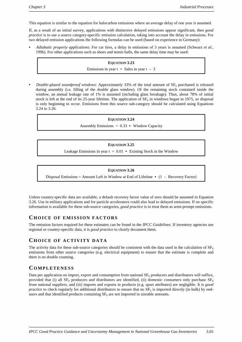
Chapter 3 Industrial Processes
IPCC Good Practice Guidance and Uncertainty Management in National Greenhouse Gas Inventories 3.65
This equation is similar to the equation for halocarbon emissions where an average delay of one year is assumed.
If, as a result of an initial survey, applications with distinctive delayed emissions appear significant, then goodpractice is to use a source category-specific emission calculation, taking into account the delay in emissions. Fortwo delayed emission applications the following formulas can be used (based on experience in Germany):
• Adiabatic property applications: For car tires, a delay in emissions of 3 years is assumed (Schwarz et al.,1996). For other applications such as shoes and tennis balls, the same delay time may be used:
EQUATION 3.23Emissions in year t = Sales in year t – 3
• Double-glazed soundproof windows: Approximately 33% of the total amount of SF6 purchased is releasedduring assembly (i.e. filling of the double glass window). Of the remaining stock contained inside thewindow, an annual leakage rate of 1% is assumed (including glass breakage). Thus, about 78% of initialstock is left at the end of its 25-year lifetime. The application of SF6 in windows began in 1975, so disposalis only beginning to occur. Emissions from this source sub-category should be calculated using Equations3.24 to 3.26:
EQUATION 3.24Assembly Emissions = 0.33 • Window Capacity
EQUATION 3.25Leakage Emissions in year t = 0.01 • Existing Stock in the Window
EQUATION 3.26Disposal Emissions = Amount Left in Window at End of Lifetime • (1 – Recovery Factor)
Unless country-specific data are available, a default recovery factor value of zero should be assumed in Equation3.26. Use in military applications and for particle accelerators could also lead to delayed emissions. If no specificinformation is available for these sub-source categories, good practice is to treat them as semi-prompt emissions.
CH O I C E O F E M I S S I O N F A C T O R SThe emission factors required for these estimates can be found in the IPCC Guidelines. If inventory agencies useregional or country-specific data, it is good practice to clearly document them.
CH O I C E O F A C T I V I T Y D A T AThe activity data for these sub-source categories should be consistent with the data used in the calculation of SF6emissions from other source categories (e.g. electrical equipment) to ensure that the estimate is complete andthere is no double counting.
CO M P L E T E N E S SData per application on import, export and consumption from national SF6 producers and distributors will suffice,provided that (i) all SF6 producers and distributors are identified, (ii) domestic consumers only purchase SF6from national suppliers, and (iii) imports and exports in products (e.g. sport attributes) are negligible. It is goodpractice to check regularly for additional distributors to ensure that no SF6 is imported directly (in bulk) by end-users and that identified products containing SF6 are not imported in sizeable amounts.
Industrial Processes Chapter 3
IPCC Good Practice Guidance and Uncertainty Management in National Greenhouse Gas Inventories3.66
DE V E L O P I N G A C O N S I S T E N T T I M E S E R I E SFor base year estimates, data may be needed for a few years prior to the base year; one year for semi-promptemissions and more years for delayed emission applications. It is good practice to calculate emissions of SF6using the same method for every year in the time series. Where data are unavailable to support a more rigorousmethod for all years in the time series, it is good practice to recalculate according to the guidance provided inChapter 7, Methodological Choice and Recalculation, Section 7 3.2.2, Alternative Recalculation Techniques.
UN C E R T A I N T Y A S S E S S M E N TIf the survey of domestic sales per application by national SF6 producers and distributors is complete, then theaccuracy of annual apparent consumption data will be high. The uncertainty in emissions estimates will besimilarly small when the uses are all semi-prompt emissions. In case of delayed emission applications theuncertainties are:
• Default delay times in adiabatic property applications: 3±1 year;
• Defaults for soundproof windows: 50±10% filling emissions and 1±0.5% leakage/breach emissions.
3.5.2.2 Reporting and documentationIt is good practice to document and archive all information required to produce the national emissions inventoryestimates as outlined in Chapter 8, Quality Assurance and Quality Control, Section 8.10.1, InternalDocumentation and Archiving. It is not practical to include all documentation in the national inventory report.However, the inventory should include summaries of methods used and references to source data such that thereported emissions estimates are transparent and steps in their calculation may be retraced.
For transparency, it is good practice to report both actual and potential emissions from the source category ‘otheruses’ separately from other SF6 emissions. In addition, providing information on the specific applications that areincluded in this source category is useful for comparing (estimates of) national practices with other countries,regionally, or globally. In addition, the methods applied and references should be documented. For delayedemission sub-source categories, annual emissions, delay times and emission factors per type of sub-sourcecategory should be reported.
3.5.2.3 Inventory quality assurance/quality control (QA/QC)It is good practice to conduct quality control checks as outlined in Chapter 8, Quality Assurance and QualityControl, Table 8.1, Tier 1 General Inventory Level QC Procedures, and an expert review of the emissionsestimates. Additional quality control checks as outlined in Chapter 8, and quality assurance procedures may alsobe applicable, particularly if higher tier methods are used to determine emissions from this source category.Inventory agencies are encouraged to use higher tier QA/QC for key source categories as identified in Chapter 7,Methodological Choice and Recalculation.
Additional procedures specific to other sources of SF6 are outlined below:
Comparison of emissions est imates using different approaches
Inventory agencies should compare total national potential SF6 emissions (minus the amount allocated to theelectrical equipment use category, the semiconductor manufacturing use category, the metal production categoryand the SF6 production category) to the estimated SF6 emissions from other uses. The potential national emissionscan be used as an upper bound on emissions.
Activity data check
Inventory agencies should compare the activity data submitted by different producers and distributors, and,adjusting for relative size or capacity of the companies, to identify significant outliers. Any outliers should beinvestigated to determine if the differences can be explained or if there is an error in the reported activity.
Comparison of emissions with other countries
Inventory agencies should compare the emissions from other SF6 end-uses included in the national inventory withinformation submitted by other similar countries. For each source, emissions per capita or per unit of GDP withother countries should be compared. If national figures appear to be relatively very high or very small, ajustification should be provided.

Chapter 3 Industrial Processes
IPCC Good Practice Guidance and Uncertainty Management in National Greenhouse Gas Inventories 3.67
3 . 5 . 3 P r o d u c t i o n o f S F 6
3.5.3.1 Methodological issuesThe IPCC Guidelines do not provide a default emission factor for inadvertent losses during production andhandling of SF6. Although these emissions are likely to be small, emissions may be significant in some countries.For example, experience in Japan indicates an emission factor of 8% of the gas produced, including handlinglosses during disposal of residual gas in returned cylinders (Suizu, 1999). This is because there is a large demandfor highly purified SF6 gas, and impure gas may be released.
CH O I C E O F M E T H O DIt is good practice to choose the method according to the decision tree in Figure 3.9, Decision Tree for SF6Production. The number of major SF6 producers is quite small: globally about 6 companies produce SF6 withabout 10 production facilities world-wide (Preisegger, 1999). The number of smaller producers may grow in thenear future, particularly in the Economies in Transition and in China. However, a survey of national producersshould not be difficult to compile. These producers should provide an estimate of their total emissions.
Emissions of SF6 may occur during production as well as handling of new gas at the site. Based on Germanexperience, a default emission factor of 0.2% of the total quantity of SF6 produced is suggested for thosecountries in which the predominant end use does not require highly purified SF6 gas (e.g. electrical equipment,insulated windows) (Preisegger, 1999). As discussed above, in countries where the major uses require highlypurified SF6 gas (e.g. semiconductor manufacturing), the default value should be 8%. If national data areavailable, these should be used.
Recycling of used gas may be done by the producers of new gas or by other recycling firms. Emissions mayoccur during handling and purification of old gas and handling of recycled gas. Specific emission factors are notavailable. Thus, good practice is to use the default factor for new production (0.2%).
UN C E R T A I N T Y AS S E S S M E N TProduction emissions can be negligible (e.g. when scrubbers capture the SF6 gas released). The estimateduncertainty range for the default emission factor is therefore 0.2±0.2 (%). Relative uncertainty of the default 8%emission factor is of the same order.
CO M P L E T E N E S SFor some inventory agencies, identifying smaller producers and, in particular, recycling firms may be a difficulttask. However, initial estimates based on the national mass balance of SF6 should identify if such entities providea sizeable contribution to total national emissions.
3.5.3.2 Reporting and documentationConfidentiality issues may arise where there are limited numbers of manufacturers. In these cases more aggregatereporting of total national SF6 applications may be necessary. If survey responses cannot be released as publicinformation, third-party review of survey data may be necessary to support data verification efforts.
It is good practice to document and archive all information required to produce the national emissions inventoryestimates as outlined in Chapter 8, Quality Assurance and Quality Control, Section 8.10.1, InternalDocumentation and Archiving. It is not practical to include all documentation in the national inventory report.However, the inventory should include summaries of methods used and references to source data such that thereported emissions estimates are transparent and steps in their calculation may be retraced.
3.5.3.3 Inventory quality assurance/quality control (QA/QC)It is good practice to conduct quality control checks as outlined in Chapter 8, Quality Assurance and QualityControl, Table 8.1, Tier 1 General Inventory Level QC Procedures, and an expert review of the emissionsestimates. Additional quality control checks as outlined in Chapter 8, quality assurance procedures may also beapplicable, particularly if higher tier methods are used to determine emissions from this source category.

Industrial Processes Chapter 3
IPCC Good Practice Guidance and Uncertainty Management in National Greenhouse Gas Inventories3.68
Inventory agencies are encouraged to use higher tier QA/QC for key source categories as identified in Chapter 7,Methodological Choice and Recalculation.
Comparison of emissions est imates using different approachesInventory agencies should compare the estimate based on aggregated producer-level data to an estimate based onnational production data and the suggested default emission factor of 0.2%. They should investigate significantdiscrepancies in cooperation with the producers to determine if there are unexplained differences.
F i g u r e 3 . 9 D e c i s i o n T r e e f o r S F 6 P r o d u c t i o n
Arethere any SF6
manufacturers in thecountry?
Report‘Not Occurring’
No
Yes
Sum datafrom plants
Box 2
Compile alist of all SF6manufacturers
Are detaileddata available on
plant-specificestimates?
Yes
Is this akey sourcecategory?(Note 1)
Estimateemissions from
SF6 plants
Box 1
No
Yes
No
Collectemissions data
from plants
Note 1: A key source category is one that is prioritised within the national inventory system because its estimate has a significantinfluence on a country’s total inventory of direct greenhouse gases in terms of the absolute level of emissions, the trend in emissions, orboth. (See Chapter 7, Methodological Choice and Recalculation, Section 7.2, Determining National Key Source Categories.)

Chapter 3 Industrial Processes
IPCC Good Practice Guidance and Uncertainty Management in National Greenhouse Gas Inventories 3.69
3 . 6 P F C , H F C , S F 6 E M I S S I O N S F R O MS E M I C O N D U C T O R M A N U F A C T U R I N G
3 . 6 . 1 M e t h o d o l o g i c a l i s s u e sThe semiconductor industry currently emits fluorocarbons (CF4, C2F6, C3F8, c-C4F8, CHF3), nitrogen trifluoride(NF3), and sulfur hexafluoride (SF6) from its manufacturing process.30 These gases, collectively referred to asfluorinated compounds (FCs), are used in two important steps of semiconductor manufacturing: (i) plasmaetching thin films and (ii) cleaning chemical vapour deposition (CVD) tool chambers. In addition, a fraction ofthe fluorocarbons used in the production process are converted into CF4.
CH O I C E O F M E T H O DEmissions vary according to the gases used in manufacturing different types of semiconductors, the process (ormore roughly, process type (CVD or etch)) used, the brand of process tool used, and the implementation ofatmospheric emission reduction technology.
The IPCC Guidelines do not provide specific guidance on how to estimate greenhouse gas emissions fromsemiconductor manufacturing. However, using the basic methodological principles outlined in the IPCCGuidelines for other source categories, four alternative methods for estimating FC emissions are described below.The use of the ‘Tier’ terminology in this section corresponds to increasing data requirements and sophisticationof the emission estimation process. The choice of methods will depend on data availability and is outlined in thedecision tree, see Figure 3.10, Decision Tree for FC Emissions from Semiconductor Manufacturing.
Continuous emissions monitoring is currently viewed as neither a technically nor economically viable means toestimate emissions from this industry. Thus, all four methods are based on gas sales/purchases data and a seriesof parameters that affect emissions. The most rigorous method, Tier 2a method, requires company-specific valuesfor the parameters rather than defaults. The Tier 2b method uses company-specific data on the share of gas usedin etching versus cleaning and the share of gas used in processes with emission control technology, but relies ondefault values for some or all of the other parameters. The Tier 2c method uses company-specific data on theshare of gas used in processes with emission control technology, but does not distinguish between etching andcleaning, and uses default values for the other parameters. The Tier 1 method uses default values for allparameters and does not account for the use of emission control technology.
Tier 2a Method – Process-specif ic parametersThis method is appropriate where company-specific or plant-specific values are available for the followingparameters: the amount of gas fed into each process or tool (or into small subsets of processes or tools), thefraction of purchased gas remaining in the shipping container after use (heel), the fraction of the gas ‘used’(destroyed or transformed) in the semiconductor manufacturing process, the fraction of the gas converted to CF4during semiconductor manufacture, the fraction of the gas fed into processes with emission control technologies,and the fraction of the gas destroyed by those emission control technologies. For purposes of transparency andcomparability, the values used for these emission parameters should be well documented (see Choice of EmissionFactors).
30Although NF3 does not currently have a global warming potential (GWP) recognized by the IPCC, NF3 emissions arediscussed in this chapter. Molina et al. have estimated a GWP-100 of 8,000 and an atmospheric lifetime of 740 years(Molina, 1995).

Industrial Processes Chapter 3
IPCC Good Practice Guidance and Uncertainty Management in National Greenhouse Gas Inventories3.70
F i g u r e 3 . 1 0 D e c i s i o n T r e e f o r F C E m i s s i o n s f r o m S e m i c o n d u c t o rM a n u f a c t u r i n g
Estimate emissionsusing the Tier 2b
method
Box 2
Is theresemiconductor
manufacturing inthe country?
Yes
No
YesCollect activity andemissions data from
semiconductorcompanies
Is this akey sourcecategory?(Note 1)
Report‘Not Occurring’
No
Do anysemi-conductor
companies use FCs in theirmanufacturing
processes?
Areactivity data and
emission factors availablefrom semiconductor
companies?
Arenational data
available on annual FCusage (purchases or sales)
by this industry?
Estimateemissions using the
Tier 1 method
Box 4
Docompanies that
report use company-specific emission
factors?
Doreporting
companies track FC gasusage by process type (i.e.
CVD clean andetch)?
Develop or obtain data onannual FC usage by semi-
conductor industry(e.g. sales data)
Estimateemissions using
the Tier 2c method
Box 3
Estimate emissionsusing the Tier 2a
method
Box 1
No
No
No
No
Yes
No
Yes Yes
Yes
Yes
Note 1: A key source category is one that is prioritised within the national inventory system because its estimate has a significantinfluence on a country’s total inventory of direct greenhouse gases in terms of the absolute level of emissions, the trend in emissions, orboth. (See Chapter 7, Methodological Choice and Recalculation, Section 7.2, Determining National Key Source Categories.)

Chapter 3 Industrial Processes
IPCC Good Practice Guidance and Uncertainty Management in National Greenhouse Gas Inventories 3.71
Emissions resulting from the use of a specific FC (FCi) consist of emissions of FCi itself plus emissions of CF4created as a by-product during the use of FCi . The following calculation should be repeated for each gas for eachprocess type:
EQUATION 3.27
Emissions of FCi = (1 – h) • ∑p
[FCi,p • (1 – Ci,p) • (1 – ai,p • di,p)]
Where:
p = Process or process type (etching or CVD chamber cleaning)
FCi,p = kg of gas i fed into process/process type p (CF4, C2F6, C3F8, C4F8, CHF3, NF3, SF6)
h = Fraction of gas remaining in shipping container (heel) after use
Ci,p = Use rate (fraction destroyed or transformed) for each gas i and process/process type p (in kgs)
ai,p = Fraction of gas volume fed into in processes with emission control technologies (company-or plant-specific)
di,p = Fraction of gas i destroyed by the emission control technology (If more than one emission controltechnology is used in process/process type p, this is the average of the fraction destroyed by thoseemission control technologies, where each fraction is weighted by the quantity of gas fed into toolsusing that technology)
EQUATION 3.28
By-product Emissions of CF4 for FCi,p = (1 – h) • ∑p
[Bi,p • FCi,p • (1 – ai,p • dCF4,p)]
Where:
Bi,p = Fraction of gas i transformed into CF4 for each process/process type
dCF4,p = Fraction of CF4 by-product destroyed by the emission control technology (e.g. control technologytype listed in Table 3.15, Default Emission Factors for HFC, PFC, and SF6 Emissions fromSemiconductor Manufacturing)
After estimating CF4 emissions for each gas, inventory agencies or companies should sum these emissions acrossall gases to arrive at an estimate of aggregate CF4 emissions.
Tier 2b Method – Process type-specif ic parametersThe Tier 2b method also uses the Equations 3.27 and 3.28. However, instead of distinguishing among processesor small sets of processes, it distinguishes only between process types (etching vs. CVD chamber cleaning).Consequently, the Tier 2b method requires data on the aggregate quantities of each gas fed into all etchingprocesses and all cleaning processes (FCi,p), as opposed to the quantities of each gas fed into each individualprocess. Industry-wide generic default values are used for any or all of the following: the fraction of the gasremaining in the shipping container (h), the fraction of the gas ‘used’ (destroyed or transformed) per process type(Ci,p), and the fraction of the gas converted into CF4 in the process type (Bi). Defaults are also presented for thefraction of the gas destroyed by the emissions control technology (di,p and dCF4,p). Company or plant-specificemission factors may be substituted for default values when available. The equations account for the plant-specific use of emission-control devices, but do not account for differences among individual processes or toolsor among manufacturing plants in their mix of processes and tools. Thus, Tier 2b estimates will be less accuratethan Tier 2a estimates.
Tier 2c Method – FC-specif ic parametersThis method calculates emissions for each FC used on the basis of company-specific data on gas sales orpurchases and on emission control technologies. It uses industry-wide generic default values for the fraction ofthe purchased gas remaining in the shipping container after use (h), the fraction of the gas ‘used’ (destroyed ortransformed) in the semiconductor manufacturing process, and the fraction of the gas converted into CF4 insemiconductor manufacture. As is the case with the Tier 2a and 2b methods, total emissions are equal to the sum

Industrial Processes Chapter 3
IPCC Good Practice Guidance and Uncertainty Management in National Greenhouse Gas Inventories3.72
of emissions from the gas FCi used in the production process plus the emissions of by-product CF4 resulting fromuse of the gas FCi., as shown in Equations 3.29 and 3.30. Unlike Tier the 2a and 2b methods, the Tier 2c methoddoes not distinguish between processes or process types.
As discussed below in the section on emission factors, the Tier 2c method uses the emission factor for the processtype (CVD or etch) in which the individual FC is most frequently used in the semiconductor industry. Thismethod reflects a current trend where individual FCs tend to be used predominantly in particular process types(CVD or etch) throughout the semiconductor industry. However, in countries with companies or plants thatdepart significantly from the industry-wide pattern of usage (e.g. by using a gas primarily in etch while othersprimarily use it in CVD), inventory agencies should evaluate the potential to introduce error by using the Tier 2cmethod rather than the Tier 2b method.
EQUATION 3.29Emissions of FCi = (1 – h) • [ FCi • (1 – Ci) • (1 – ai • di)]
Where:
FCi = Sales/purchases of gas i in kg (CF4, C2F6, C3F8, c-C4F8, CHF3, NF3, SF6)
h = Fraction of gas remaining in shipping container (heel) after use
Ci = Use rate of gas (fraction destroyed or transformed in process)
ai = Fraction of gas i volume used in processes with emission control technologies (company- or plant-specific)
di = Fraction of gas i destroyed by the emission control technology
EQUATION 3.30By-product Emissions of CF4 for FCi = (1 – h) • [(Bi • FCi) • (1 – ai • dCF4
)]
Where:
Bi = kg CF4 created per kg of gas i used
dCF4 = Fraction of CF4 by-product destroyed by the emission control technology
After estimating CF4 emissions for each gas, inventory agencies or companies should sum these emissions acrossall gases to arrive at an estimate of aggregate CF4 emissions.
This method does not account for differences among process types (etching versus cleaning), individualprocesses, or tools.
Tier 1 Method – DefaultThe Tier 1 method is the least accurate estimation method. It should be used only in cases where company-specific data are not available. This method calculates emissions for each FC used on the basis of national gassales or purchase data. It uses industry-wide generic default values for: the fraction of the purchased gasremaining in the shipping container after use, the fraction of the gas ‘used’ (transformed or destroyed) in thesemiconductor manufacturing process, and the fraction of the gas transformed into CF4 in semiconductormanufacture. As is the case with the Tier 2 method, emissions are equal to the sum of emissions from the gas FCiused in the production process plus the emissions of by-product emissions of CF4 resulting from use of the gasFCi., as shown in Equations 3.31 and 3.32.
EQUATION 3.31Emissions of FCi = (1 – h) • [FCi • (1 – Ci)]
Where:
FCi = Sales/purchases of gas i in kg (CF4, C2F6, C3F8, c-C4F8, CHF3, NF3, SF6)
h = Fraction of gas remaining in shipping container (heel) after use
Ci = Use rate of gas (fraction destroyed or transformed in process)

Chapter 3 Industrial Processes
IPCC Good Practice Guidance and Uncertainty Management in National Greenhouse Gas Inventories 3.73
EQUATION 3.32Emissions of CF4 for FCi = (1 – h) • (Bi • FCi)
Where:
Bi = kg CF4 created per kg of gas i
After estimating CF4 emissions for each gas, inventory agencies or companies should sum them across all gasesto arrive at an estimate of aggregate CF4 emissions.
This method does not account for differences among process types (etching versus cleaning), individualprocesses, or tools. It also does not account for the possible use of atmospheric emission-control devices.
CH O I C E O F E M I S S I O N F A C T O R SAs discussed above, emissions factors based on simple semiconductor production variables are not adequate toaccount for all of the factors that influence emissions. Data for each of the following parameters are necessary toprepare a rigorous estimate:
• The gases used;
• The process type (CVD or etch) used;
• The brand of process tool used;
• Atmospheric emission reduction technology.
Default values have been developed for the parameters used in Tier 1, Tier 2b and 2c methods that reflect theliterature and expert judgement (see Table 3.15, Default Emission Factors for HFC, PFC and SF6 Emissions fromSemiconductor Manufacturing). Given the difficulty in representing the diverse production conditions within thesemiconductor industry, default emission parameters are inherently uncertain. Accuracy can be improved withlarger sets of measured data and where factors are applied to similar processes using similar or identical chemicalrecipes. Emission factors for destruction (abatement) technologies are acknowledged as currently having greateruncertainty and variability than those for the manufacturing processes. Rapid technical innovation by chemicaland equipment suppliers, and semiconductor manufacturers is expected to result in major emission reductionswithin this industry over the next 10 years. These innovations are also likely to affect emission factors. Thesemiconductor industry has established a mechanism through the World Semiconductor Council to evaluateglobal emission factors. Inventory agencies may wish to periodically consult with the industry to betterunderstand global and national circumstances.
The default value for the fraction of gas remaining in the shipping container (heel) is 0.10.

Industrial Processes Chapter 3
IPCC Good Practice Guidance and Uncertainty Management in National Greenhouse Gas Inventories3.74
TABLE 3.15DEFAULT EMISSION FACTORS FOR HFC, PFC AND SF6 EMISSIONS FROM SEMICONDUCTOR MANUFACTURING
CF4 C2F6 CHF3 C3F8 c-C4F8 NF3 SF6
Tier 1
1 – Ci 0.8 0.7 0.3 0.4 0.3 0.2 0.5
B NA 0.1 NA 0.2 NA NA NA
Tier 2c
1 – Ci 0.8 0.7 0.3 0.4 0.3 0.2 0.5
B NA 0.1 NA 0.2 NA NA NA
Tier 2b
Etch 1 – Ci 0.7 0.4 0.3 0.4 0.3 0.3a 0.5
CVD 1 – Ci 0.8 0.7 NA 0.4 ND 0.2 0.2
Etch B NA 0.1 NA ND NA NA NA
CVD B NA 0.1 NA 0.2 NA NA NA
Emission ControlTechnology (d)
CF4 C2F6 CHF3 C3F8 c-C4F8 NF3 SF6
Tier 2cb 0.9 0.9 0.9 0.9 0.9 0.9 0.9
Tier 2b
Hot Tubec 0.1 0.3 NT NT NT 0.5 0.1
Fueled combustiond 0.9 0.9 0.9 0.9 0.9 0.9 0.9
Plasma (withadditive H20vapour)e
0.9 NT 0.9 NT 0.9 0.9 0.9
Plasma (withadditive O2)
0.9 NT 0.9 NT 0.9 0.8 0.8
Catalyticf 0.9 0.9 0.9 0.9 0.9 0.9 0.9
Cryogenicabsorption
0.7 0.9 0.9 NT NT NT 0.9
MembraneSeparation
0.8 0.9 NT NT NT NT 0.9
a Use of NF3 in the etch process is typically small compared to CVD. The aggregate emissions of NF3 from etch and CVD under Tier 2bwill usually not be greater than estimates made with Tier 2c or Tier 1 methods.b Tier 2c emission control technology factors are applicable only to fueled combustion, plasma, and catalytic devices that are specificallydesigned to abate FCs. Under the Tier 2c approach, other technologies, such as hot tubes, are assumed to have a destruction efficiency of0%.Sources:c SEMATECH Technology Transfer Report, SEMATECH, 1994.d Vendor data verified by semiconductor manufacturers.e Draft SEMATECH Technology Transfer Report, SEMATECH, 1999.f Data for catalytic, cryogenic absorption and membrane separation as presented at Semicon SW 1999, Austin, Texas, USA.NA = not applicable, ND = no data, NT = not tested.

Chapter 3 Industrial Processes
IPCC Good Practice Guidance and Uncertainty Management in National Greenhouse Gas Inventories 3.75
PROCESS TOOL EMISSION FACTORSThe procedures for calculating process tool emission factors for Tier 1, Tier 2c and Tier 2b methods areidentical. Process tool emission factors are defined as the amount of greenhouse gas emitted divided by theamount of greenhouse gas used in the process. The emission factors correspond to the ‘(1 – Ci)’ term in the Tier 1and Tier 2 formulas. For example, the emission factor of 0.8 for CF4 (see Table 3.15 above, Tier 1 value) meansthat 80% of the CF4 used in the process is emitted as CF4. By-product emission factors were also calculated. Theexpert group determined that the only by-product emission of significance was that of CF4. It was furtherdetermined that the only gases that emit significant amounts of CF4 as a by-product are C2F6 and C3F8. As a resultof this discussion, CF4 by-product emission factors were calculated only for C2F6 and C3F8. For example, a valueof 0.2 for C3F8 (taken from Table 3.15 above, Tier 1 value) means that 20% of the C3F8 used is converted intoCF4.
In order to calculate the Tier 2b process tool emission factors, data were collected from the process equipmentmanufacturers and semiconductor manufacturers. The data were collected according to process type (eitherChemical Vapor Deposition (CVD) or etch) and also by type of gas (e.g. C2F6, CF4). The methods used toconduct the emissions testing were real time Quadrupole Mass Spectrometry (QMS) and Fourier TransformInfrared Spectroscopy (FTIR). Calibration standards (usually 1% mixtures with a balance of N2) were used toquantify the results. The quality analysis and quality control requirements that were followed are outlined in the‘Equipment Environmental Characterisation Guidelines’ Revision 3. The emission factors for Tier 2b (see Table3.15 above) are the simple average of the data collected for each gas for etch and CVD, rounded to onesignificant figure.
In order to determine the Tier 1 and Tier 2c process tool emission factors, some knowledge of the amounts of gasused in typical semiconductor manufacturing processes is required. The Tier 1 and Tier 2c emission factors wereobtained by determining for each of the gases which process type (CVD or etch) uses the most gas. For example,the Tier 2b emission factors for SF6 are 0.5 (etch) and 0.2 (CVD). Since the predominant use of SF6 in thesemiconductor industry is in the etch processes, the Tier 2b etch emission factor was used for the Tier 1 SF6emission factor.
For Tier 2a emission factors, semiconductor manufacturers use company or fab-specific values rather than usingdefault values as listed in Table 3.15 above.31 In order to assure the quality of emission factors, emission testingshould be conducted in accordance with accredited methods.32 If a third-party supplier conducts the emissionstesting, the semiconductor manufacturer should make sure that the third-party supplier is capable of meeting allof the requirements outlined in Revision 3.0 of the Equipment Environmental Characterisation Guidelines.Semiconductor manufacturers who use emission factors provided by the process tool equipment supplier shouldmake sure that the emission factors are applicable to their specific manufacturing process. Manufacturingmethods with process parameters (e.g. pressure, flow rate) that deviate from centreline conditions may havedifferent emission factors than those provided by the tool manufacturer.33
EMISSION CONTROL TECHNOLOGY FACTORS
Tier 2b Emission FactorsAssumptions for the emissions control technology emission factors for the Tier 2b methods include:
(i) Results listed are for actual fab emissions testing, no lab results were included;
(ii) Plasma abatement is applicable to etch tools only (less than or equal to 200mm);
(iii) Capture/Recovery (cryogenic absorption and membrane separation) emission factors are for thecapture portion of process only, recovery efficacy must be further characterised;
(iv) Cost of ownership and applicability of various technologies vary widely;
(v) Applicability of various technologies to emission from >200 mm wafer processes was notcharacterised.
31 ‘Fab-specific’ means specific to a fabrication plant.
32 One example of an internationally accredited testing method can be found in the latest version of the SemiconductorIndustry Association (2000) ‘Equipment Environmental Characterisation Guidelines’ (Revision 3.0 as of February 2000)’.
33 Centreline conditions refer to the conditions under which equipment manufacturers standardise their equipment for sale. Itis common for semiconductor manufacturers to modify these conditions to optimise for particular needs.

Industrial Processes Chapter 3
IPCC Good Practice Guidance and Uncertainty Management in National Greenhouse Gas Inventories3.76
The values presented in Table 3.15, Default Emission Factors for HFC, PFC and SF6 Emissions fromSemiconductor Manufacturing, are the average of all of the data received for each type of technology and inputgas, rounded down to the next 10% (e.g. an average of 98% would be rounded down to 0.9). The averages wererounded down to reflect that (i) emissions control devices vary in their efficacy depending upon what gas they areoptimised to destroy, and (ii) the efficacy of emission control devices on new tools processing larger wafers(>200 mm) is not well characterised. An emission control device that can destroy 99% of a FC when it isoptimised to destroy that FC on a certain tool may destroy less than 95% of that FC when it is optimised todestroy something else or when it is used on a tool for which it was not designed.
Emissions control technologies, while currently not widely deployed in the industry, are developing at a rapidpace. Default control technology emission factors in Table 3.15, Default Emission Factors for HFC, PFC and SF6Emissions from Semiconductor Manufacturing, are based on limited testing of control devices in a small subsetof processes and tools. Results are expected to vary across tools and gas flow rates. In addition, individualabatement technologies are not applicable to all tools or processes in semiconductor manufacturing facilities.
Tier 2c Emission FactorsThe emission control technology factors listed for Tier 2c were calculated from data received from equipmentsuppliers, abatement suppliers and semiconductor manufacturers. Again, the values are the average of all of thedata received for each type of input gas, rounded down to the next 10% It should be noted that only data fromabatement devices that were specifically designed to abate FCs were used in the average calculation. Data werereceived from combustion abatement devices (all of which used some type of fuel), plasma abatement devices,and catalytic abatement devices. Default control technology emission factors for Tier 2c should be used only foremissions control technologies specifically designed and installed to reduce FC emissions. If companies use anyother type of abatement device, such as a hot tube, they should assume that its destruction efficiency is 0% underthe Tier 2c method. Emissions control technologies are expected to evolve over time and emission factors shouldbe re-evaluated periodically.
CH O I C E O F A C T I V I T Y D A T AActivity data for this industry consists of data on gas sales, purchases, or use. For the more data-intensive Tier 2methods, gas purchase data at the company or plant-level are necessary. For the Tier 1 method, it is preferablethat company-level gas purchase data are used. Where purchase data are not available, sales data may beavailable from the gas manufacturers or distributors. Sales data should include only the share of each gas that issold to the semiconductor industry. It may be necessary to make assumptions about this share if the data are notavailable from gas manufacturers or distributors.
UN C E R T A I N T Y A S S E S S M E N TUse of the Tier 2a method will result in the least uncertain inventory and the Tier 1 method is the most uncertain.Given the limited number of plants and the close monitoring of production processes at the plant level, collectionof data for use in Tier 2b or Tier 2a methods should be technically feasible. The Tier 1 method has the greatestlevel of uncertainty. Inventory agencies should seek the advice of the industry on uncertainties, using theapproaches to obtaining expert judgement outlined in Chapter 6, Quantifying Uncertainties in Practice.
CO M P L E T E N E S SComplete accounting of emissions from the semiconductor industry should be achievable in most countriesbecause there are a limited number of companies and plants. There are four issues related to completeness thatshould be addressed:
• Other by-products: A number of transformation by-products are generated as a result of FC use forchamber cleaning and etching. With the exception of CF4, however, FC by-product concentrations areassumed to be negligible. Inventory agencies should re-evaluate this assumption if new gases are adopted bythe industry.
• New chemicals: Completeness will be an issue in the future as the industry evaluates and adopts newchemical processes to improve its products. Industry-wide efforts to reduce FC emissions are alsoaccelerating the review of new chemicals. Consequently, good practice for this industry is to incorporate amechanism that accounts for greenhouse gases not listed in the IPCC Second Assessment Report (e.g. NF3,C5F8, HFEs). These new gases may also produce high GWP by-products.

Chapter 3 Industrial Processes
IPCC Good Practice Guidance and Uncertainty Management in National Greenhouse Gas Inventories 3.77
• Other sources: A small amount of FCs may be released during gas handling (e.g. distribution) and bysources such as research and development (e.g. university) scale plants and tool suppliers. These emissionsare not believed to be significant (e.g. less than 1% of this industry’s total emissions).
• Other products or processes: FC use has been identified in the electronics industry in emissive applicationsincluding: manufacture of flat panel displays34 and hard disk drives reliability testing (inert liquids),coolants35 (direct evaporative cooling for electric and electronic apparatuses and indirect coolants in closedcircuit of electric and electronic apparatuses), vapour phase reflow soldering, and precision cleaning.36
DE V E L O P I N G A C O N S I S T E N T T I M E S E R I E SUse of FCs by the semiconductor industry began in the late 1970s and accelerated significantly beginning in theearly 1990s. Determining a base year emissions level may present difficulties because few data are available foremissions occurring before 1995. If historical emissions estimates were based on simple assumptions (e.g. useequals emissions), then these estimates could be improved by applying the methods described above. If historicaldata are not available to permit use of a Tier 2 method, then the Tier 1 method using default emission parameterscan be used retrospectively. Both Tier 1 and Tier 2 could then be applied simultaneously for the years in whichmore data become available to provide a comparison or benchmark. This should be done according to theguidance provided in Chapter 7, Methodological Choice and Recalculation, Section 7.3.2.2, AlternativeRecalculation Techniques.
In order to ensure a consistent emissions record over time, an inventory agency should recalculate FC emissionsfor all years reported whenever emissions calculation procedures are changed (e.g. if an inventory agencychanges from the use of default values to actual values determined at the plant level). If plant-specific data arenot available for all years in the time series, the inventory agency will need to consider how current plant data canbe used to recalculate emissions for these years. It may be possible to apply current plant-specific emissionparameters to sales data from previous years, provided that plant operations have not changed substantially. Sucha recalculation is required to ensure that any changes in emission trends are real and not an artefact of changes inprocedure.
3 . 6 . 2 R e p o r t i n g a n d d o c u me n t a t i o nIt is good practice to document and archive all information required to produce the national emissions inventoryestimates as outlined in Chapter 8, Quality Assurance and Quality Control, Section 8.10.1, InternalDocumentation and Archiving. It is not practical to include all documentation in the national inventory report.However, the inventory should include summaries of methods used and references to source data such that thereported emissions estimates are transparent and steps in their calculation may be retraced.
Explicit reporting on emissions in this industry would improve the transparency and comparability of emissions.For example, under Table 2F of the IPCC reporting tables an additional line should be added for semiconductormanufacturing emissions. As a number of FCs gases are emitted by this industry, reporting by individual gasspecies rather than by chemical type would also improve the transparency and usefulness of this data. Efforts toincrease transparency should take into account the protection of confidential business information related tospecific gas use. Country-level aggregation of gas-specific emissions data should protect this information incountries with three or more manufacturers. Table 3.16, Information Necessary for Full Transparency ofEstimates of Emissions from Semiconductor Manufacturing, shows the supporting information necessary for fulltransparency in reported emissions estimates.
Good practice for Tier 2a is to document the development of company-specific emission factors, and to explainthe deviation from the generic default values. Given confidentiality concerns, inventory agencies may wish toaggregate this information across manufacturers. In cases where manufacturers in a country have reported
34 Emissions from flat panel display (thin film transistor (TFT) liquid crystal) manufacturing may be estimated usingmethods similar to those used for semiconductor manufacturing. Company-specific emission and abatement factors arerequired. Very small amounts are also used in microelectronic machine (MEM) manufacturing and research and developmentlaboratories/facilities.
35 Emissions from ‘hard disc drives reliability testing’ and ‘coolants’ are to be accounted for in Section 3.7.6, OtherApplications Sub-source Category.
36 Emissions from precision cleaning are to be accounted for in Section 3.7.2, Solvents Sub-source Category.

Industrial Processes Chapter 3
IPCC Good Practice Guidance and Uncertainty Management in National Greenhouse Gas Inventories3.78
different emission or conversion factors for a given FC and process or process type, inventory agencies mayprovide the range of factors reported and used.
Until handling of NF3, C5F8, HFEs, and other FC gases is decided upon, emissions should be reported separatelyand not included in total emissions calculations.
TABLE 3.16INFORMATION NECESSARY FOR FULL TRANSPARENCY OF ESTIMATES OF EMISSIONS FROM
SEMICONDUCTOR MANUFACTURING
Data Tier 1 Tier 2c Tier 2b Tier 2a
Emissions of each FC (rather than aggregated for all FCs) X X X X
Sales/purchases of each FC X X
Mass of each FC used in each process or process type X X
Fraction of each FC used in processes with emission control technologies X X X
Use rate for each FC for each process or process type (This and followinginformation is necessary only if default value is not used)
X
Fraction of each FC transformed into CF4 for each process or process type X
Fraction of gas remaining in shipping container X
Fraction of each FC destroyed by emission control technology X
Fraction of CF4 by-product destroyed by emission control technology X
3 . 6 . 3 I n v e n t o r y q u a l i t y a s s u r a n c e / q u a l i t y c o n t r o l( Q A / Q C )
It is good practice to conduct quality control checks as outlined in Chapter 8, Quality Assurance and QualityControl, Table 8.1, Tier 1 General Inventory Level QC Procedures, and an expert review of the emissionsestimates. Additional quality control checks as outlined in Chapter 8, and quality assurance procedures may alsobe applicable, particularly if higher tier methods are used to determine emissions from this source category.Inventory agencies are encouraged to use higher tier QA/QC for key source categories as identified in Chapter 7,Methodological Choice and Recalculation.
Additional general guidance for higher tier QA/QC procedures is also included in Chapter 8. Due to the highlycompetitive nature of the semiconductor industry, provisions for handling confidential business informationshould be incorporated into the verification process. Methods used should be documented, and a periodic audit ofthe measurement and calculation of data should be considered. A QA audit of the processes and proceduresshould also be considered.

Chapter 3 Industrial Processes
IPCC Good Practice Guidance and Uncertainty Management in National Greenhouse Gas Inventories 3.79
3 . 7 E M I S S I ON S OF S U B S T I T U T E S F ORO ZO N E D E P L E T I N G S U S B S T A N C E S ( O D SS U B S T I T U T E S )
O v e r v i e w ( 3 . 7 . 1 t o 3 . 7 . 7 )This chapter provides good practice guidance on seven sources of emissions of substitutes for ozone depletingsubstances (ODS). Each of the following uses is discussed in a separate section:
• Aerosols and metered dose inhalers;
• Solvent uses;
• Foam;
• Stationary refrigeration;
• Mobile air conditioning;
• Fire protection;
• Other applications.
G e n e r a l me t h o d o l o g i c a l i s s u e s f o r a l l O D Ss u b s t i t u t e s s u b - s o u r c e c a t e g o r i e s
CH O I C E O F M E T H O DThe IPCC Guidelines describe two tiers for estimating emissions from the use of ODS substitutes: the advancedor actual method (Tier 2), and the ‘basic’ or ‘potential’ method (Tier 1).37 The actual method (Tier 2) accountsfor the time lag between consumption and emissions of ODS substitutes, whereas the potential method assumesthat emissions occur during the year in which the chemical is produced or sold into a particular end-use sector.
While the Tier 1 method requires less data, it may produce very inaccurate estimates over the short term because,for many long-lived sources such as refrigerators, chemicals are emitted over a period of several years. Thegreater the length of time over which the chemical is released, the greater the possible inaccuracy of the‘potential’ method. If, as is the case in most countries, equipment sales are increasing each year, the total amountof chemical stored in end-use equipment must also be increasing. Therefore, the potential method is likely tooverstate emissions
Good practice is to use the Tier 2 actual method for all sub-source categories within this source category.Consistency requires that inventory agencies make every attempt to apply actual methodologies across the wholespectrum of ODS substitute emission sources. If an inventory agency is unable to implement actual methods forall sub-source categories, it is good practice to calculate and report potential estimates for all sub-sourcecategories to allow the summation of total emissions. Actual and potential emissions estimates should not besummed together by the inventory agency.
The generalised decision tree in Figure 3.11, Generalised Decision Tree for All Substitutes for Ozone DepletingSubstances, describes good practice in choosing between Tier 2 and Tier 1 methods for each end-use in the sevensub-sections that follow. Good practice is to use the Tier 2 method for those sub-source categories that wereidentified as ‘key sub-source categories’ as discussed in Chapter 7, Methodological Choice and Recalculation.This determination is done at the level of the IPCC source category level (in this case ‘ODS Substitutes’) and notat the level of the IPCC sub-source category.
37 The Conference of the Parties to the UNFCCC, at its third session, affirmed ‘… that the actual emissions ofhydrofluorocarbons, perfluorocarbons and sulphur hexafluoride should be estimated, where data are available, and used forthe reporting of emissions. Parties should make every effort to develop the necessary sources of data;’. (Decision 2/CP.3,Methodological issues related to the Kyoto Protocol)

Industrial Processes Chapter 3
IPCC Good Practice Guidance and Uncertainty Management in National Greenhouse Gas Inventories3.80
F i g u r e 3 . 1 1 G e n e r a l i s e d D e c i s i o n T r e e f o r A l l S u b s t i t u t e s f o rO z o n e D e p l e t i n g S u b s t a n c e s
AreODS substitutes
used in anyapplications?
Report‘Not Occurring’
No
Are dataavailable for Tier 2
actual emissions fromthe use of each
HFC/PFC?
Use default Tier 2emission parametersfor each individual
substance
Box 2
Yes
Is this akey sourcecategory?(Note 1)
Areproduction
and import/export dataavailable for each
HFC/ PFC?
Arecountry-specific
emission parametersavailable?
Obtain thenecessary data forthe Tier 2 method
Use country-specificTier 2 emission
parameters for eachindividual substance
Box 3
Use the Tier 1potential emission
approach
Box 1
Obtainproduction andimport/exportdata for each
HFC/PFC
Yes
No No No
YesYes
Yes
No
Note 1: A key source category is one that is prioritised within the national inventory system because its estimate has a significantinfluence on a country’s total inventory of direct greenhouse gases in terms of the absolute level of emissions, the trend in emissions, orboth. (See Chapter 7, Methodological Choice and Recalculation, Section 7.2, Determining National Key Source Categories.)

Chapter 3 Industrial Processes
IPCC Good Practice Guidance and Uncertainty Management in National Greenhouse Gas Inventories 3.81
The good practice guidance in this section deals with variations of the Tier 2 method, rather than implementingthe potential method. Each sub-section discusses how to apply these methods to specific ODS sub-sourcecategories, reviews existing data sources, and identifies gaps therein. For further guidance on implementing theTier 1 method, countries can refer to Section 2.17.3 of the IPCC Guidelines, Vol. 3.
In general, it is good practice to develop appropriate country data for the Tier 2 method when the emissions fromthe ODS replacement source categories are a significant component of the national inventory. This may require acountry-specific model. More detailed decision trees are included for each sub-source category to assist in thefurther identification of data needs and selection of the Tier 2 approach.
Inventory agencies implementing the Tier 2 method will need to determine whether to use bottom-up or top-down approaches. The bottom-up approach takes into account the time lag between consumption and emissionsexplicitly through emission factors. The top-down approach takes the time lag into account implicitly, by trackingthe amount of virgin chemical consumed in a given year that is used to replace chemical that was emitted to theatmosphere.
Tier 2a – Bottom-up approachThe bottom-up method is based on the number of products and end-uses where ODS substitutes are consumedand emitted. This approach estimates the number of equipment units that use these chemicals, average chemicalcharges, average service life, emission rates, recycling, disposal, and other pertinent parameters. Annualemissions are then estimated as a function of these parameters through the life of the units. Since equipment unitsvary significantly in the amount of chemical used, service life, and emission rates, the characterisation of thisequipment can be a resource intensive task. The longer-lived the end-use equipment, and the more diverse thetypes of equipment within a particular application, the more complex the bottom-up approach has to be in orderto account for emissions.38 The bottom-up approach can provide an accurate estimate of emissions if the datacalled for by the following equation are available for all relevant types and vintages of equipment:
EQUATION 3.33Total Emissions of Each PFC or HFC = Equipment Assembly Emissions + Equipment Operation
Emissions + Equipment Disposal Emissions
Assembly emissions occur as fugitives when equipment is filled or refilled with a chemical. Emissions fromequipment also occur as leaks, or intentional releases during operation. Finally, when the equipment life ends andit is disposed, the remaining charge of HFC/PFC escapes to the atmosphere, is recycled, or possibly destroyed.
The need to update equipment inventories on an annual basis can be a major implementation challenge forinventory agencies with limited resources. The bottom-up method does not require annual chemical consumptiondata, however, although it could be used as a quality assurance check if available.
Tier 2b – Top-down approachThe top-down approach also estimates emissions from assembly, operation, and disposal, but does not rely onemission factors. Instead, the method uses measured consumption (i.e. sales) of each chemical in the country orfacility being considered. The general equation is as follows39:
Equation 3.34Emissions = Annual Sales of New Gas – (Total Charge of New Equipment
– Original Total Charge of Retiring Equipment)
Industry purchases new chemical from manufacturers to replace leakage (i.e. emissions) from the currentequipment stock, or to make a net change in the size of the total charge of the equipment stock.40 The total
38 As approximately twenty different HFC and PFC chemicals could potentially be used as substitutes for ozone depletingsubstances, and emissions sources are numerous and extremely diversified, implementing the bottom-up method involvesdealing with high volumes of data and levels of complexity.
39 Boundary conditions: If there is no net change in the total equipment charge, then annual sales are equal to emissions. Ifthe net change in the total equipment charge is equal to annual sales, then emissions are zero.

Industrial Processes Chapter 3
IPCC Good Practice Guidance and Uncertainty Management in National Greenhouse Gas Inventories3.82
charge of new equipment minus the original total charge of retiring equipment represents the net change tocharge of the equipment stock. Where the net change is positive, some of the new chemical is being used tosatisfy the increase in the total charge, and therefore cannot be said to replace emissions from the previous year.
Using this approach, it is not necessary to know the total amount of each chemical in equipment stock in order tocalculate emissions. One only needs to know the total charges of the new and retiring equipment. This approachis most directly applicable to the refrigeration and mobile air conditioning, and fire protection sub-sourcecategories. Further elaboration and modification of this approach is provided in the description of each sub-source category. In addition, models are being developed that allocate chemical sales for different end uses intodifferent regions of the world. These models are currently being derived for specific ODS Substitute end usessuch as foam and fire protection.41
CH O I C E O F E M I S S I O N F A C T O R SThe type of emission factor required depends on the Tier 2 approach implemented.
Tier 2a – Bottom-up approachFor the bottom-up approach, specific emission factors are required to estimate emission rates from the majorequipment types and sectors. Emission factors should be based on a country-specific study of the equipment unitsin stock to determine their remaining service lives, average charges, retrofit rates, leak rates, disposal quantities,and recovery practices. The IPCC Guidelines include default values for some of these parameters, but these arenot country-specific. Good practice guidance provides additional default values for some sub-source categories.
A common theme is that management of the disposal of equipment at the end of its service life can have aprofound effect on the total emissions. The chemical remaining in systems (called the ‘bank’) can be up to 90%of the original quantity used. Specific issues related to emission factors are discussed in the sub-source categorysections.
Tier 2b – Top-down approachAs discussed above, the top-down approach generally relies on chemical sales data and does not use equipment-based emission factors. Where there are exceptions to this rule, good practice guidance is provided in each sub-source category section (e.g. fugitive emissions during the filling of equipment with HFCs and PFCs).
CH O I C E O F A C T I V I T Y D A T A
Tier 2a – Bottom-up approachThe bottom-up approach requires an inventory of existing HFC/PFC in existing units (i.e. the ‘bank’). Someinventory agencies may have access to national data published in trade magazines or technical reports. However,it is more likely that a study will be necessary to estimate the inventory of existing units or chemicals. Expertpanels can also facilitate the generation of this information. Inventory agencies may also decide to conductannual studies to update their inventories of sector units. An alternative to this may be to calculate or estimateproduction growth for each one of the sub-source categories under consideration. Data need to reflect new unitsthat are introduced each year, and old or poorly functioning units that are retired.
Tier 2b – Top-down approachActivity data for the top-down approach focus on chemical deployment rather than sources of emissions. Forcertain end-uses, such as fire protection and foam, global models are being developed that allocate accuratelyknown production data into end-uses in specific regions. The activity data from these models will be particularlyuseful for countries with significant imports of chemical and equipment.
For the sales-based approach, data on national chemical use are more easily obtained than data for the nationalinventory of equipment responsible for emissions. It is good practice to obtain data on the total annual sales fromthe gas manufacturers or importers.42 The best source of data on the total charge of new equipment is likely to be
40 Industry also requires new chemical to replace destroyed gas and for stockpiles. Terms can be added to the generalequation to account for these uses; these terms are not included here for simplicity.
41 For example, see www.greenhousegases.org.
42 Tier 1b method of the IPCC Guidelines, Vol. 3, Section 2.17.3.3, provides the default method for annual sales data.

Chapter 3 Industrial Processes
IPCC Good Practice Guidance and Uncertainty Management in National Greenhouse Gas Inventories 3.83
the equipment manufacturers or the trade associations that represent them. For the total charge of retiringequipment, one must know or estimate (i) equipment lifetime, and (ii) either (a) the historical sales of equipmentand the equipment’s historical average charge size, or (b) the growth rate of such sales and charge sizes.
Inventory agencies in countries that import all or the majority of new chemicals consumed are likely to encounterdifferent issues of data availability than those in countries with significant domestic chemicals production. If themajority of chemicals are imported, either in bulk or in equipment and products, some form of import data willbe necessary for calculating emissions. Ideally, customs officials should track and make available chemicalimport statistics. For some products, such as foam and aerosols, it may not be possible for customs officials totrack the type of chemical in the product (e.g. CFCs vs. HFCs in aerosols), or the presence of the product in theimported equipment (e.g. closed cell foam in automobile seats). In such cases, it may be necessary to collect orestimate data with the assistance of major distributors and end-users.
CO M P L E T E N E S SCompleteness, in terms of the total quantity of chemical that could potentially be emitted, is covered by the factthat activity data for the top-down approach are recorded in terms of the quantity of chemical used. Completenessis an important issue for countries that use the Tier 2 bottom-up equipment-based method.
A fraction of new chemical production escapes to the atmosphere during production of each substance. Fugitiveemissions from production are not accounted for in either of the Tier 2 methods (or the Tier 1 method). It is goodpractice for inventory agencies in countries with domestic chemical production to include fugitive emissions intheir inventories. The suggested approach is to apply an emission factor to chemical production, or to assume thata fixed (additional) percentage of chemical sales was emitted during production. Although the default factor is0.5%, experience in Japan shows much larger emissions.43 It is good practice to determine the actual emissionfactor for each plant.
DE V E L O P I N G A C O N S I S T E N T T I M E S E R I E SInventory agencies that have prepared potential (Tier 1) estimates in the past are encouraged to develop thecapacity to prepare Tier 2 estimates in the future. It is good practice that actual and potential estimates are not tobe included in the same time series, and that inventory agencies recalculate historical emissions with the actualmethod, if they change approaches. If data are unavailable, the two methods should be reconciled to ensureconsistency, following the guidance on recalculation provided in Chapter 7, Methodological Choice andRecalculation, Section 7.3.2.2, Alternative Recalculation Techniques. It is good practice to fully documentrecalculation, ensuring transparency.
Emission factors generally come from historical data on other chemicals (e.g. CFCs) used in established marketsand need to be adapted to new chemicals (e.g. ODS substitutes) in start-of-life markets. National data on baseyear deployment is now available (or can be calculated with known uncertainty).
UN C E R T A I N T Y AS S E S S M E N TOver a long time (greater than 20 years) emissions of ODS substitutes within a country will tend to equal totalconsumption in the same time frame. For a given year, the quantification of uncertainty for ODS is very difficultto estimate, due to the large number of different sources and the diversity of emission patterns. For the top-downTier 2 method, the overall uncertainty will be directly related to quality and completeness of chemical sales andimport data. For the bottom-up Tier 2 method, the uncertainty will reflect the completeness of the equipmentsurvey, and the appropriateness of the emission functions developed to characterise emissions. Further advice onuncertainties is provided in the separate sections on the seven sub-source categories that follow.
R e p o r t i n g a n d d o c u me n t a t i o n f o r a l l O D Ss u b s t i t u t e s s u b - s o u r c e c a t e g o r i e sIt is good practice to document and archive all information required to produce the national emissions inventoryestimates as outlined in Chapter 8, Quality Assurance and Quality Control, Section 8.10.1, InternalDocumentation and Archiving.
43 Source: The Sixth Meeting of the Committee for Prevention of Global Warming and The Chemical Products Council ofJapan, 21 May 1999.

Industrial Processes Chapter 3
IPCC Good Practice Guidance and Uncertainty Management in National Greenhouse Gas Inventories3.84
As discussed above, inventory agencies should prepare and report actual emissions estimates for as many end usesub-source categories as possible. For those sub-source categories where it is not possible to prepare actualemissions estimates, inventory agencies should prepare and report potential emissions estimates. Inventoryagencies reporting an actual/potential hybrid approach should include a set of potential estimates for each sub-source category so that total ODS substitute emissions can be calculated. As noted above, actual and potentialestimates should not be summed together.
The balance between preservation of confidentiality and transparency of the data needs to be carefully addressed.Careful aggregation may solve some problems but will require that results are validated by other means (e.g. thirdparty audit). Where data have been aggregated to preserve the confidentiality of proprietary information,qualitative explanations should be provided to indicate the method and approach for aggregation.
I n v e n t o r y q u a l i t y a s s u r a n c e / q u a l i t y c o n t r o l( Q A / Q C ) f o r a l l O D S s u b s t i t u t e s s u b - s o u r c ec a t e g o r i e sIt is good practice to conduct quality control checks as outlined in Chapter 8, Quality Assurance and QualityControl, Table 8.1, Tier 1 General Inventory Level QC Procedures, and an expert review of the emissionsestimates. Additional quality control checks as outlined in Chapter 8, and quality assurance procedures may alsobe applicable, particularly if higher tier methods are used to determine emissions from this source categories.Inventory agencies are encouraged to use higher tier QA/QC for key source categories as identified in Chapter 7,Methodological Choice and Recalculation. In addition to the guidance in Chapter 8, specific procedures ofrelevance to this source category are outlined below.
Comparison of emissions est imates using different approaches
Inventory agencies should use the Tier 1 potential emissions method for a check on the Tier 2 actual estimates.Inventory agencies may consider developing accounting models that can reconcile potential and actual emissionsestimates and may improve determination of emission factors over time.
Inventory agencies should compare bottom-up estimates with the top-down Tier 2 approach, since bottom-upemission factors have the highest associated uncertainty. This technique will also minimise the possibility thatcertain end-uses are not accounted for in the bottom-up approach.
National act ivity data check
For the Tier 2a (bottom-up) method, inventory agencies should evaluate the QA/QC procedures associated withestimating equipment and product inventories to ensure that they meet the general procedures outlined in theQA/QC plan and that representative sampling procedures were used. This is particularly important for the ODSsubstitutes sub-sectors because of the large populations of equipment and products.
For the Tier 2b (top-down) method, inventory agencies should evaluate and reference QA/QC proceduresconducted by the organisations responsible for producing chemical deployment information. Sales data maycome from gas manufacturers, importers, distributors, or trade associations. If the QC associated with thesecondary data is inadequate, then the inventory agency should establish its own QC checks on the secondarydata, reassess the uncertainty of the emissions estimates derived from the data, and reconsider how the data areused.
Emission factors check
Emission factors used for the Tier 2a (bottom-up) method should be based on country-specific studies. Inventoryagencies should compare these factors with the default values. They should determine if the country-specificvalues are reasonable, given similarities or differences between the national source category and the sourcerepresented by the defaults. Any differences between country specific factors and default factors should beexplained and documented.

Chapter 3 Industrial Processes
IPCC Good Practice Guidance and Uncertainty Management in National Greenhouse Gas Inventories 3.85
3 . 7 . 1 A e r o s o l s s u b - s o u r c e c a t e g o r y
3.7.1.1 Methodological issuesMost aerosol packages contain hydrocarbon (HC) as propellants but, in a small fraction of the total, HFCs andPFCs may be used as propellants or solvents. Emissions from aerosols usually occur shortly after production, onaverage six months after sale. During the use of aerosols, 100% of the chemical is emitted (Gamlen et al., 1986,USA EPA, 1992a). The 5 main sources are as follows:
(i) Metered Dose Inhalers (MDIs);
(ii) Personal Care Products (e.g. hair care, deodorant, shaving cream);
(iii) Household Products (e.g. air-fresheners, oven and fabric cleaners);
(iv) Industrial Products (e.g. special cleaning sprays, lubricants, pipe-freezers);
(v) Other General Products (e.g. silly string, tire inflators, claxons).
The HFCs currently used as propellants are HFC-134a, HFC-227ea, and HFC-152a. The substanceHFC-43-10mee and a PFC, perfluorohexane, are used as solvents in industrial aerosol products.44
CH O I C E O F M E T H O DAerosol emissions are considered ‘prompt’ because all the initial charge escapes within the first year or two aftersale. Therefore, to estimate emissions it is necessary to know the total amount of aerosol initially charged inproduct containers prior to sale. Emissions of each individual aerosol in year t can be calculated according to theIPCC Guidelines as follows:
Equation 3.35Emissions of HFCs in year t =
[(Quantity of HFC and PFC Contained in Aerosol Products Sold in year t) • (EF)] + [(Quantity of HFC and PFC Contained in Aerosol Products Sold in year (t – 1)] • (1 – EF)]
This equation should be applied to each chemical individually. Total carbon equivalent emissions are equal to thesum of the carbon equivalent emissions of each chemical.
Since the lifetime of the product is assumed to be two years, any amount not emitted during the first year must bydefinition be emitted during the second and final year. In reality, most emissions occur within the first year ofproduct purchase, but this calculation accounts for the lag period from time of purchase to time of use.45 Adecision tree for estimating actual emissions is included in Figure 3.12, Decision Tree for Actual Emissions (Tier2) from the Aerosol Sub-source Category. The data collection process is described below.
44 HFC-43-10mee is used solely as a solvent, but is counted as an aerosol when delivered through aerosol canisters.
45 For short-lived sources such as MDIs and aerosol products, the estimate of potential emissions is equivalent to using anemission factor of 100%. This will produce a result similar to the actual approach if there is no substantial growth in aerosolsales.

Industrial Processes Chapter 3
IPCC Good Practice Guidance and Uncertainty Management in National Greenhouse Gas Inventories3.86
F i g u r e 3 . 1 2 D e c i s i o n T r e e f o r A c t u a l E m i s s i o n s ( T i e r 2 ) f r o m t h eA e r o s o l S u b - s o u r c e C a t e g o r y
Does thecountry produce
aerosol products andmetered dose inhalers
(MDIs) containingHFCs and
PFCs?
Are salesdata available from
local manufacturers ofaerosol products and MDIs
containing HFCsand PFCs?
Calculate emission of eachsubstance in each end-use,using bottom-up sales datafrom aerosol product andMDI manufacturers, foreach product category
In each year, for eachindividual substance,
obtain data from HFC/PFCproducers and importers
for gas sales for MDIs andother aerosol products
Calculate emissionsof each substance
using top-down data
Box 2
Yes
NoAre aerosol
product and MDIimport statistics
available?
Calculate emissions fromimported products for each
chemical using aerosolproduct import data
Box 3
Obtain data from majorend-users or distributors
of products andcalculate emissions from
imported products
Box 4
No
Yes Yes
No
Box 1

Chapter 3 Industrial Processes
IPCC Good Practice Guidance and Uncertainty Management in National Greenhouse Gas Inventories 3.87
CH O I C E O F E M I S S I O N F A C T O R SIt is good practice to use a default emission factor of 50% of the initial charge per year for the broad spectrum ofaerosol products. This means that half the chemical charge escapes within the first year and the remaining chargeescapes during the second year (Gamlen et al., 1986). Inventory agencies should use alternative emission factorsonly when empirical evidence is available for the majority of aerosol products. In any event, the percentageemission factors should in general sum to 100% over the time during which it is assumed that the charge willescape. The development of country-specific emission factors should be documented thoroughly. General aerosoland MDI manufacturers may be able to provide data on process losses.
CH O I C E O F A C T I V I T Y D A T AThe activity data required are the total quantity of each relevant chemical contained in all aerosol productsconsumed within a country (both domestic sales and imports). For countries that import 100% of aerosolproducts, activity data are equal to imports.
Activity data for this end use sub-source category can be collected using either a bottom-up or a top-downapproach, depending on the availability and quality of the data. The bottom-up approach requires data on thenumber of aerosol products sold and imported (e.g. number of individual metered dose inhalers, hair careproducts, and tire inflators), and the average charge per container. The top-down approach involves collectingaerosol and MDI chemical sales data directly from chemical manufacturers. In many cases, a mix of bottom-upand top-down data may be necessary.
Domestic aerosol production: For countries with domestic production, general aerosol and MDI manufacturerscan provide data on the quantity of aerosol products produced for consumption in the country, the number ofaerosols exported, the average charge per aerosol, and the type of propellant or solvent used (i.e. whichHFC/PFC). Total use of domestically produced aerosol products in each year can then be calculated as thenumber of aerosol products sold domestically in a given year times the charge of HFC/PFC in each product. Ifbottom-up data are not available, domestic chemical producers can provide data on the amount of HFCs sold todomestic manufacturers in metered dose inhalers, and aggregate sales data to producers of other aerosols(categories 2, 3, 4 and 5 above). If domestic aerosol and MDI manufacturers import HFCs, information may alsobe sought from chemical exporters, although they may not be able to provide data on exports destined forindividual countries because of confidential business concerns. Customs officials and chemical distributors areanother possible source for chemical import data.
Imported aerosol production: Most countries will import a significant share of their total aerosol products.Data on imports of HFC-containing general aerosols may be difficult to collect because official import statisticsfor aerosol products do not typically differentiate HFC-containing aerosols from others. When usable importstatistics are unavailable from customs agencies, data may be available from product distributors and specificend-users. For example, in the case of MDIs, a limited number of pharmaceutical companies typically importproducts, and these companies can be surveyed to obtain the required information.
CO M P L E T E N E S SCompleteness depends on the availability of activity data. Inventory agencies in countries without domesticaerosol production may need to use expert judgement in estimating activity data, because import statistics arelikely to be incomplete (see Chapter 6, Quantifying Uncertainties in Practice, Section 6.2.5, Expert Judgement).
DE V E L O P I N G A C O N S I S T E N T T I M E S E R I E SEmissions from aerosols should be calculated using the same method and data sources for every year in the timeseries. Where consistent data are unavailable for any year in the time series, gaps should be recalculatedaccording to the guidance provided in Chapter 7, Methodological Choice and Recalculation, Section 7.3.2.2,Alternative Recalculation Techniques.
UN C E R T A I N T Y A S S E S S M E N TThe use of HFCs in the general aerosol sector is larger than in the MDI sector. Data from HFC manufacturers andimporters of sales to the general aerosol sector are, at the present time, not well defined other than for HFC-134aon a global scale. These data can be improved through additional data collection activities. The diffuse nature ofthe general aerosol sector means that the acquisition of reliable bottom-up data requires specific study on acountry basis through local industry experts, whose advice should be sought on uncertainties using theapproaches to expert judgement outlined in Chapter 6, Quantifying Uncertainties in Practice.

Industrial Processes Chapter 3
IPCC Good Practice Guidance and Uncertainty Management in National Greenhouse Gas Inventories3.88
There are several sources of reliable data for the MDI sector, leading to a high level of confidence in the datareported that should be reflected in inventory emissions estimates. However, in reporting for a single country, theabsence of reliable data for the general aerosol sector could mean that emission data could be over or underestimated by a factor of between one third and three times.
3.7.1.2 Reporting and documentationThe emission estimate for metered dose inhalers should be reported separately from the emission estimate forother aerosols. Inventory agencies should document the emission factor used. If a country-specific emissionfactor rather than the default factor is used, its development should be documented. Detailed activity data shouldbe reported to the extent that it does not disclose confidential business information. Where some data areconfidential, qualitative information should be provided on the types of aerosol products consumed, imported,and produced within the country. It is likely that the type of HFC used as a propellant or solvent and the sales ofMDIs and general aerosols into individual countries could be viewed as confidential.46 Where there are less thanthree manufacturers of specific chemicals used as solvents, reporting could be aggregated into this section,because both are considered 100% emissive applications (see Section 3.7.2.2 below).
3.7.1.3 Inventory quality assurance/quality control (QA /QC)
It is good practice to conduct quality control checks as outlined in Chapter 8, Quality Assurance and QualityControl, Table 8.1, Tier 1 General Inventory Level QC Procedures, and an expert review of the emissionsestimates. Additional quality control checks as outlined in Chapter 8, Section 8.7, Source Category-specific QCProcedures (Tier 2), and quality assurance procedures may also be applicable, particularly if higher tier methodsare used to determine emissions from this source category. Inventory agencies are encouraged to use higher tierQA/QC for key source categories as identified in Chapter 7, Methodological Choice and Recalculation.
In addition to the guidance in Chapter 8, Quality Assurance and Quality Control, specific procedures of relevanceto this sub-source category are outlined as follows. Both bottom-up and top-down data should be used as a checkon the emission estimate. Data used to calculate emissions from year t–1 should be consistent with data used inthe previous year’s inventory estimate, so the two-year total sums to 100%. If this is not the case, then the reasonfor the inconsistency should be reported. Collection of the data described in the section on data collection aboveshould provide adequate quality control. To allow independent assessment of the level of quality of the datareporting, the number of manufacturers of aerosols plus end users should be quantified.
46 Quantification of use data for individual general aerosol sectors will enable more reliable future projections to bedeveloped and emission reduction strategies to be considered.

Chapter 3 Industrial Processes
IPCC Good Practice Guidance and Uncertainty Management in National Greenhouse Gas Inventories 3.89
3 . 7 . 2 S o l v e n t s s u b - s o u r c e c a t e g o r y
3.7.2.1 Methodological issuesHFCs and PFCs are used as solvents in four main areas as follows:
(i) Precision Cleaning;
(ii) Electronics Cleaning;
(iii) Metal Cleaning;
(iv) Deposition applications.
The use of HFCs as solvents is still in its infancy. Solvents that have been or may be used include HFC43-10mee,perfluorohexane (a PFC) and others that were not listed in the IPCC Second Assessment Report, includingHFC-365mfc.47
CH O I C E O F M E T H O DAs is the case in the aerosol sector, emissions from solvent applications generally are considered ‘prompt’emissions because 100% of the chemical is emitted within two years. To estimate emissions it is necessary toknow the total amount of chemical in solvent products sold each year. Emissions of HFCs and PFCs from solventuse in year t can be calculated according to the IPCC Guidelines as follows.
EQUATION 3.36Emissions in year t = [(Quantity of Solvents Sold in year t) • EF]
+ [Quantity of Solvents Sold in year (t – 1) • (1 – EF)]
As with aerosols, the equation should be applied to each chemical individually, depending on the disaggregationin available data. Moreover, the equation may also be applied to different equipment classes. Total carbonequivalent emissions are equal to the sum of carbon equivalent emissions of each chemical.
The emission factor EF represents the fraction of chemical emitted from solvents in year t. The product lifetime isassumed to be two years, and thus any amount not emitted during the first year must by definition be emittedduring the second and final year. A decision tree for estimating actual emissions is included in Figure 3.13,Decision Tree for Actual Emissions (Tier 2) from the Solvents Sub-source Category. The data collection processis described below.
CH O I C E O F E M I S S I O N F A C T O R SGood practice is to use a default emission factor of 50% of the initial charge/year for solvent applications.48 Incertain applications with new equipment, it is possible that much lower loss rates will be achieved and thatemissions will occur over a period of more than two years. Alternative emission factors can be developed in suchsituations, using bottom-up data on the use of such equipment and empirical evidence regarding alternativeemission factors.49 Such country-specific emission factors should be documented thoroughly.
Modifications for the recovery and recycling of solvents should not be applied. While HFC and PFC solventsmay be recovered and recycled several times during their use due to their high costs, in most emissive end usesthe chemical will be released on average six months after sale.
47 The IPCC Guidelines provide ‘Reporting Instructions’ only for greenhouse gases with global warming potentials listed inthe Second Assessment Report.
48 See footnote 47.
49 As guidance, for sales to new equipment, approximately 10-20% will be emitted with the rest of the gas banked. Insubsequent years sales are for servicing volumes and can be considered 100% emitted.

Industrial Processes Chapter 3
IPCC Good Practice Guidance and Uncertainty Management in National Greenhouse Gas Inventories3.90
CH O I C E O F A C T I V I T Y D A T AThe activity data for this end-use are equal to the quantity of each relevant chemical sold as solvent in a particularyear. As with aerosols, data on both domestic and imported solvent quantities should be collected. The requireddata can be collected using either top-down or bottom-up methods, depending on the character of the nationalsolvent industry. In most countries, the end-users will be extremely diverse and a top-down approach would bepractical.
F i g u r e 3 . 1 3 D e c i s i o n T r e e f o r A c t u a l E m i s s i o n s ( T i e r 2 ) f r o m t h eS o l v e n t s S u b - s o u r c e C a t e g o r y
AreODS substitutes
used as solvents inthe country?
Do asmall number oflarge companiesdominate solvent
consumption?
Report‘Not Occurring’
Calculate emissionsof each HFC/PFC
using top-down salesand import data
No
YesBox 1
Isthere any
domestic solventproduction?
In each year, for eachindividual substance,
obtain data from HFC/PFCproducers and importersfor gas sales to solvent
producers
Areequipment and
solvent consumption dataavailable directly from
companies?
In each year, for eachindividual substance,obtain solvent importdata customs statisticsor solvent distributors
Areemission factors
and activity data availablefor newer equipment
with lower leakrates?
Calculate emissions of eachHFC/PFC in each end-use,using bottom-up sales data
and default emission factors
Calculate emissions of eachHFC/PFC in each end-use,using bottom-up sales data,new emission factors where
available, and defaultfactors for the remainder
No
No
NoNo
No
Yes
Yes
Yes
Yes
Box 3
Box 2

Chapter 3 Industrial Processes
IPCC Good Practice Guidance and Uncertainty Management in National Greenhouse Gas Inventories 3.91
Top-down dataTop-down data are equal to the amount of chemical solvent sold or imported annually into a country. Domesticsolvent sales should be available directly from chemical manufacturers. As solvents are only produced in a fewcountries, most countries will import some or all of their consumption. Data on imported solvents can becollected from the exporting manufacturers, although information on exports to individual countries may beconsidered confidential. Alternatively, import statistics from customs agencies or the distributors of importedsolvents can be used. Solvent import data are generally more easily obtained than aerosol import data becausesolvent is usually imported in bulk rather than in small containers.
If specific emission factors are developed for particular types of equipment, it will be necessary to disaggregatethe consumption data into these equipment classes. In general, this will require a bottom-up approach.
Bottom-up dataBottom-up activity data include the number of pieces of equipment or canisters containing solvent and theircharge. The bottom-up approach is suitable where large corporations consume most of the solvent sold, becauseit should be possible to obtain detailed solvent end-use data from a few large entities. The bottom-up approachmay also be most appropriate when equipment-specific emission factors are available.
CO M P L E T E N E S SCompleteness depends on the availability of activity data. Inventory agencies in countries without domesticsolvent production may need to use expert judgement in estimating activity data, because import statistics arelikely to be incomplete (see Chapter 6, Quantifying Uncertainties in Practice, Section 6.2.5, Expert Judgement).
DE V E L O P I N G A C O N S I S T E N T T I M E S E R I E SEmissions from foam should be calculated using the same method and data sources for every year in the timeseries. Where consistent data are unavailable for any years in the time series, gaps should be recalculatedaccording to the guidance provided in Chapter 7, Methodological Choice and Recalculation.
UN C E R T A I N T Y AS S E S S M E N TThe default assumption that all solvent is emitted within two years is widely accepted and should not lead to asignificant error. Similarly, the activity data should be reliable because of the small number of chemicalmanufacturers, the high cost of the gas leading to little stockpiling, and the 100% emissive nature of the use inmost applications.
3.7.2.2 Reporting and documentationInventory agencies should report the emission factor used, and the empirical basis for any country-specificfactors. For activity data, chemical sales and imports should be reported, unless there are confidentiality concernsdue to the limited number and location of manufacturers. (At present, for example, there may be only oneproducer of each compound.) Where there are less than three manufacturers of specific chemicals used assolvents, reporting could be aggregated into the aerosol section, because both are considered 100% emissiveapplications (see Section 3.7.1.2 above). In this case, to preserve confidentiality, emissions of individual gasesshould not be specified and emissions should be reported in CO2-equivalent tonnes.
3.7.2.3 Inventory quality assurance/quality control (QA/QC)It is good practice to conduct quality control checks as outlined in Chapter 8, Quality Assurance and QualityControl, Table 8.1, Tier 1 General Inventory Level QC Procedures, and an expert review of the emissionsestimates. Additional quality control checks as outlined in Chapter 8, Section 8.7, Source Category-specific QCProcedures (Tier 2), and quality assurance procedures may also be applicable, particularly if higher tier methodsare used to determine emissions from this source category. Inventory agencies are encouraged to use higher tierQA/QC for key source categories as identified in Chapter 7, Methodological Choice and Recalculation.
In addition to the guidance in Chapter 8, Quality Assurance and Quality Control, specific procedures of relevanceto this source category are outlined below:

Industrial Processes Chapter 3
IPCC Good Practice Guidance and Uncertainty Management in National Greenhouse Gas Inventories3.92
• For accurate quality control/assurance both top-down and end-use data should be compiled. To allowindependent assessment of the level of quality of the data reporting, the number of manufacturers anddistributors plus end users interviewed should be quantified.
• When applying emission factors and activity data specific to various solvent applications, the activity datashould be obtained at the same level of detail.

Chapter 3 Industrial Processes
IPCC Good Practice Guidance and Uncertainty Management in National Greenhouse Gas Inventories 3.93
3 . 7 . 3 F o a m s u b - s o u r c e c a t e g o r y
3.7.3.1 Methodological issuesIncreasingly, HFCs are being used as replacements for CFCs and HCFCs in foam applications such as insulating,cushioning, and packaging. Compounds that may be used include HFC-245fa, HFC-365mfc, HFC-134a, andHFC-152a. For open-cell foam, emissions of HFCs used as blowing agents are likely to occur during themanufacturing process. In closed-cell foam, emissions occur over a longer time period (e.g. 20 years).
CH O I C E O F M E T H O DThe decision tree in Figure 3.14, Decision Tree for Actual Emissions (Tier 2) from the Foam Sub-sourceCategory, describes good practice methods in estimating emissions.
The IPCC Guidelines suggest calculating emissions from open-cell foam separately from emissions from closed-cell foam:
Open-Cell Foam: Since HFCs and PFCs used for open-cell foam blowing are released immediately, all of theemissions will occur in the country of manufacture. Emissions are calculated according to the following equation,as presented in the IPCC Guidelines:50
Equation 3.37Emissions from Open-cell Foam = Total Annual HFCs and PFCs Used
in Manufacturing Open-cell Foam
Closed-Cell Foam: Emissions from closed-cell foam occur at three distinct points:
(i) First Year Losses from Foam Manufacture and Installation: These emissions occur where theproduct is manufactured.
(ii) Annual Losses (in-situ losses from foam use): Closed-cell foam will lose a fraction of their initialcharge each year until decommissioning. These emissions occur where the product is used.
(iii) Decommissioning Losses: Emissions upon decommissioning also occur where the product is used.
Section 2.17.4.3 of the IPCC Guidelines, Vol.3, Estimation of Emissions of HFCs and PFCs from FoamBlowing, presents an equation for calculating emissions from the foam blowing that accounts for the first twoemission points. In order to prepare a complete estimate of emissions from this source, it is good practice to adda third term to the equation to account for decommissioning losses and chemical destruction, where data areavailable. Thus, the suggested equation is:
Equation 3.38Emissions from Closed-cell Foam = [(Total HFCs and PFCs Used in Manufacturing New Closed-
cell Foam in year t) • (first-year Loss Emission Factor)]+ [(Original HFC or PFC Charge Blown into Closed-cell Foam Manufacturing between year t and
year t – n) • (Annual Loss Emission Factor)] + [(Decommissioning Losses in year n) – (HFC or PFC Destroyed)]
Where:
n = Product lifetime of closed-cell foam
Decommissioning losses = the remaining chemical at the end of service life that occur when the losses equipment is scrapped
50 For these applications, actual emissions of each chemical are equal to potential emissions.

Industrial Processes Chapter 3
IPCC Good Practice Guidance and Uncertainty Management in National Greenhouse Gas Inventories3.94
This equation should be applied to each chemical and major foam application individually. Total CO2-equivalentemissions are equal to the sum of CO2-equivalent emissions of each combination of chemical type and foamapplication.
To implement this approach it is necessary to collect current and historical data on annual chemical sales to thefoam industry for the period up to and including the average lifetime of closed-cell foam (e.g. the most recenttwenty years). If it is not possible to collect data for potential losses upon decommissioning, it should be assumedthat all chemical not emitted in manufacturing is emitted over the lifetime of the foam.
A modification of this approach is to use activity data provided by a global model that allocates accurately knownproduction data to the different foam applications in various regions around the world. These data can then beused with the disaggregated emission factors provided in Table 3.17, Default Emission Factors for HFC/PFCfrom Closed-Cell Foam.

Chapter 3 Industrial Processes
IPCC Good Practice Guidance and Uncertainty Management in National Greenhouse Gas Inventories 3.95
F i g u r e 3 . 1 4 D e c i s i o n T r e e f o r A c t u a l E m i s s i o n s ( T i e r 2 ) f r o m t h eF o a m S u b - s o u r c e C a t e g o r y
CH O I C E O F E M I S S I O N F A C T O R SAs in other sub-source categories, the first choice for emission factors is to develop and use peer-reviewed andwell documented country-specific data based on field research. As noted previously, if no information isavailable for decommissioning losses, then the emission factors used for first-year and annual losses shouldaccount for all chemical consumption.51
51 It has also been noted that decommissioning may not necessarily involve total loss of blowing agent at that point, eitherbecause of a level of secondary use or because the item has been discarded intact (e.g. many refrigerators). These could beconsidered as some of the end-of-life management options available to nations, but are clearly less effective than properdestruction or recovery technologies. Future emission models should focus proper attention to end-of-life issues.
Are ODSsubstitutes used in
the foam sub-sourcecategory in the
country?
Report‘Not Occurring’
No
Yes
Perform an end-usesurvey to determinefoam applicationsused in the country
AreTier 2 activity
data available fromglobal model?
Canactivity data bedisaggregated
by foamtype?
Are detailedcountry-specific
emission parameters availableby foam type? (e.g. product
life, first yearlosses)
Calculate emissions by substanceand foam type, using nationaldata, disaggregated country-
specific parameters, and the Tier2 equation, incorporating end of
life data if available
Calculate emissions bysubstance, using national
data, general defaultparameters, and the Tier 2
equation, incorporatingend of life data if available
Calculate emissions bysubstance and foam type, using
national data, disaggregateddefault parameters, and the Tier2 equation, incorporating end of
life data if available
Collect or estimatenational activity
data
No
Yes
No
Yes
No
Yes
Box 3
Box 1 Box 2

Industrial Processes Chapter 3
IPCC Good Practice Guidance and Uncertainty Management in National Greenhouse Gas Inventories3.96
If country-specific data are not available, default assumptions can be used. Table 3.18, Default Emission Factorsfor HFC-134a Applications (Foam Sub-source Category) – (Derived from existing CFC/HFC informationaccumulated through national/international research), and Table 3.19, Default Emission Factors for HFC-245a/HFC-365mfc Applications (Foam Sub-source Category) – (Derived from existing CFC/HFC informationaccumulated through national/international research), present state-of-the-art good practice emission factorsassumptions for the most important current closed-cell foam applications. Use of these factors will require dataon chemical sales and the bank of chemical in equipment for these applications.
If only aggregated chemical sales data for closed-cell foam are available and information on specific foam typescannot be obtained, the general default emission factors listed in the IPCC Guidelines should be used.52 Thesegeneral default emission factors are shown in Table 3.17, Default Emission Factors for HFC/PFC from Closed-Cell Foam.
TABLE 3.17DEFAULT EMISSION FACTORS FOR HFC/PFC FROM CLOSED-CELL FOAM
Emission Factor Default Values
Product Lifetime n = 20 years
First Year Losses 10% of the original HFC or PFC charge/year, although the value could drop to 5% ifsignificant recycling takes place during manufacturing.
Annual Losses 4.5% of the original HFC or PFC charge/year
Source: Gamlen et al. (1986).
TABLE 3.18DEFAULT EMISSION FACTORS FOR HFC-134A APPLICATIONS (FOAM SUB-SOURCE CATEGORY)
(DERIVED FROM EXISTING CFC/HFC INFORMATION ACCUMULATED THROUGH NATIONAL/INTERNATIONAL RESEARCH)
HFC-134a Applications Product Life in years First Year Loss % Annual Loss %
Polyurethane – Integral Skina 12-15 95 2.5
Polyurethane – Continuous Panel 50 10 0.5
Polyurethane – Discontinuous Panel 50 12.5 0.5
Polyurethane – Appliance 15-20 7.5 0.5
Polyurethane – Injected 15 12.5 0.5
One Component Foam (OCF) a 50 95 2.5
Extruded Polystyrene/Polyethylene (XPS/PE) a
50 40 3
a HFC-152a Applications.
Source: Ashford (1999).
52 No emission factors are provided for open-cell foams because all emissions occur during the first year.

Chapter 3 Industrial Processes
IPCC Good Practice Guidance and Uncertainty Management in National Greenhouse Gas Inventories 3.97
TABLE 3.19DEFAULT EMISSION FACTORS FOR HFC-245A/HFC-365MFC APPLICATIONS (FOAM SUB-SOURCE CATEGORY) –
(DERIVED FROM EXISTING CFC/HFC INFORMATION ACCUMULATED THROUGH NATIONAL/INTERNATIONAL RESEARCH)
HFC-245a/HFC-365mfc Applications Product Life in years First Year Loss % Annual Loss %
Polyurethane – Continuous Panel 50 7.5 0.5
Polyurethane – Discontinuous Panel 50 10 0.5
Polyurethane – Appliance 15 4 0.25
Polyurethane – Injected 15 10 0.5
Polyurethane – Continuous Block 15 40 0.75
Polyurethane – Discontinuous Block 15 45 0.75
50 10 1
Polyurethane – Continuous Laminate 25 10 1
Polyurethane – Spray 50 25 1.5
Phenolic – Discontinuous Block 15 45 0.75
Phenolic – Discontinuous Laminate 50 10 1
Source: Ashford (1999).
Use of these default emission factors will result in 90% of the initial charges being emitted over twenty years ofannual use, after the initial 10% during the first year.
CH O I C E O F A C T I V I T Y D A T ATwo types of activity data are needed in order to prepare the emissions estimates: the amount of chemical used infoam manufacturing in a country, and the amount of chemical contained in foam used in the country. Datacollection issues related to these two areas differ.
• Chemical Used in Foam Manufacture: The amount of bulk chemicals used in the foam blowing industryshould include both domestically produced and imported HFCs and PFCs. Domestic chemical sales data tothe foam industry should be available directly from chemical manufacturers. As with other ODS substitutesub-source categories, imported chemical data may be available from customs officials or chemicaldistributors.
For open-cell foam, all emissions will occur during manufacture. Thus, it is necessary to determine the share ofchemical associated with the manufacture of open-celled foam. These data can be determined through an end-usesurvey, or approximated by reviewing similar end-use data gathered on CFCs and HCFCs.
• Chemical Emitted During the Lifetime of Closed-Cell Foam: Annual decommissioning losses associatedwith closed-cell foam should be calculated for all the foam in use in the country. This will requireconsideration of the import and export of products containing closed-cell foam which can be quitecomplicated.
Inventory agencies in countries that export closed-cell foam should subtract these volumes from their calculationsof annual and decommissioning losses, since the emissions will occur in the importing country. Data on thechemical charge of exported closed-cell foam may be available from large manufacturers.
Inventory agencies in countries that import products containing closed-cell foam, in contrast, should includeestimates of emissions from these imported products for completeness. Since import statistics for closed-cellfoam products are extremely difficult to collect, inventory agencies in countries whose emissions occur only fromimported closed-cell foam may need to use expert judgement in estimating this data (see Chapter 6, QuantifyingUncertainties in Practice, Section 6.2.5, Expert Judgement).
In the future, inventory agencies may be able to use international HFC/PFC production and consumption data setsto develop estimates of chemical contained in imported closed-cell foam. For example, the AlternativeFluorocarbon Environmental Assessment Study (AFEAS) statistics-gathering process compiled global activity

Industrial Processes Chapter 3
IPCC Good Practice Guidance and Uncertainty Management in National Greenhouse Gas Inventories3.98
data up until 1997 for HFC-134a in the foam sector.53 Although the global data are relatively well understood,regional breakdowns are not presently available.
CO M P L E T E N E S SFifteen foam applications and four potential chemicals used as blowing agents (HFC-134a, HFC-152a,HFC-245fa and HFC-365mfc) have been identified in the foam sub-source category. For completeness, inventoryagencies should determine whether the blowing agents are used in each application, which suggests 60theoretically possible combinations (see Table 3.20, Use of ODS Substitutes in the Foam Blowing Industry). Inpractice, this list reduces to 32 realistic potential chemical/application combinations, although there are somepotential regional variations. It should also be noted that, at this stage, the method does not address the potentialuse of blends and, in reality, it would be difficult to assign different emission factors to such systems. The mainproblem with the potential use of blends will be one of activity monitoring.
TABLE 3.20USE OF ODS SUBSTITUTES IN THE FOAM BLOWING INDUSTRY(FOAM PRODUCT EMISSIONS BY GAS – ODS REPLACEMENTS)
HFC Foam Blowing Agent AlternatesbSub-sectors
HFC-134a HFC-152a HFC-245fa HFC-365mfc
PUa Flexible Foam X X X X
PU Flexible Molded Foam X X X X
PU Integral Skin Foam Ο Ο X X
PU Continuous Panel Ο X Ο Ο
PU Discontinuous Panel Ο X Ο Ο
PU Appliance Foam Ο X Ο Ο
PU Injected Foam Ο X Ο Ο
PU Continuous Block X X Ο Ο
PU Discontinuous Block X X Ο Ο
PU Continuous Laminate X X Ο Ο
PU Spray Foam X X Ο Ο
PU One Component Foam Ο Ο X X
ExtrudedPolystyrene/Polyethylene
Ο Ο X X
Phenolic Block X X Ο Ο
Phenolic Laminate X X Ο Οa PU = Polyurethane.b X – no anticipated use, Ο – current or anticipated use.
DE V E L O P I N G A C O N S I S T E N T T I M E S E R I E SAn inventory agency should maintain a consistent method in assessing its emissions over the time period. If, forexample, no system is established to monitor actual decommissioning at the outset of the inventory process, itwill be very difficult to obtain data retrospectively if a change from 'default' to 'actual' data is considered. Thisdecision should therefore be the subject of careful consideration at the outset of the reporting process. Anyrecalculation of estimates should be done according to the guidance provided in Chapter 7.
UN C E R T A I N T Y A S S E S S M E N TCurrent sales data indicate that the global estimates are accurate to within 10%, regional estimates are in the30-40% range, and the uncertainty of country specific top-down information may be more than 50% (McCulloch, 53 HFC-134a is the most commonly used HFC. AFEAS data can found at http://www.afeas.org.
Chapter 3 Industrial Processes
IPCC Good Practice Guidance and Uncertainty Management in National Greenhouse Gas Inventories 3.99
1986). The application of emission factors will add to the uncertainties, particularly if only default emissions canbe used, although it should be noted that the calculation of the total emissions for a year will be only partiallydependent on the accuracy of assumptions for new consumption in that year. The remainder of the emissions willarise from installed foam and from those decommissioned in that year. Since decommissioning will be the triggerfor the majority of emissions in many cases, the product life assumptions may introduce the greatest degree ofuncertainty in the default emissions calculations. It is therefore very important that inventory agencies keeprecords of their estimates of HFC containing products and develop some mechanism for monitoring actualdecommissioning if possible. These records may help ensure that the summed emissions do not exceed totalinputs over time.
3.7.3.2 Reporting and documentationEmissions factors should be reported, along with documentation for the development of country-specific data.Chemical sales to the foam blowing industry should be reported in a manner that preserves confidential businessinformation. Most confidentiality issues arising from any data collection process relate to the most highlyconcentrated activities. To deal with this, emissions from foam could be reported as a single number, providedthat the development of the number could be reviewed under suitable terms of confidentiality. Of course, adeclaration of consolidated emissions from manufacture (first year), use (product life) and decommissioning(end-of-life) will always be preferable to allow continued focus on improvements being made in each of theseareas. If, in the future, inventory agencies use the global and regional data sets, they should report the results ofhow they allocated emissions to the country level.
3.7.3.3 Inventory quality assurance/quality control (QA/QC)It is good practice to conduct quality control checks as outlined in Chapter 8, Quality Assurance and QualityControl, Table 8.1, Tier 1 General Inventory Level QC Procedures, and an expert review of the emissionsestimates. Additional quality control checks as outlined in Chapter 8, Section 8.7, Source Category-specific QCProcedures (Tier 2), and quality assurance procedures may also be applicable, particularly if higher tier methodsare used to determine emissions from this source category. Inventory agencies are encouraged to use higher tierQA/QC for key source categories as identified in Chapter 7, Methodological Choice and Recalculation.
One of the main concerns will be to ensure that the preservation of the integrity of regional and global data willbe maintained by the summation of individual country estimates and a major part of the QA/QC review processwill need to concern itself with this cross reference.
Industrial Processes Chapter 3
IPCC Good Practice Guidance and Uncertainty Management in National Greenhouse Gas Inventories3.100
3 . 7 . 4 S t a t i o n a r y r e f r i g e r a t i o n s u b - s o u r c ec a t e g o r y
3.7.4.1 Methodological issuesHFCs and PFCs are used as replacements for CFCs and HCFCs in refrigeration and stationary air conditioningequipment. Examples of refrigeration equipment include household refrigerators, retail food refrigeration,commercial and residential air conditioning, and cold storage warehouses. For the time being this sub-sourcecategory also includes transport refrigeration, other than that covered in the Mobile Air-conditioning sub-sourcecategory (see Section 3.7.5, Mobile Air-conditioning Sub-source Category).54
CH O I C E O F M E T H O DThe Tier 2 approach in the IPCC Guidelines is based on calculating emissions from assembly, operation, anddisposal of stationary refrigeration equipment. The general equation is shown below:
EQUATION 3.39Total Emissions = Assembly Emissions + Operation Emissions + Disposal Emissions
• Assembly emissions include the emissions associated with product manufacturing, even if the products areeventually exported.
• Operation emissions include annual leakage from equipment stock in use as well as servicing emissions.This calculation should include all equipment units in the country, regardless of where they weremanufactured.
• Disposal emissions include the amount of refrigerant released from scrapped systems. As with operationemissions, they should include all equipment units in the country where they were scrapped, regardless ofwhere they were manufactured.
Good practice is to implement a top-down Tier 2 approach, using annual sales of refrigerant. The alternativeapproach, using bottom-up equipment data and multiple emission factors, is much more data intensive and isunlikely to improve accuracy, but it is still good practice under certain national circumstances. The decision treein Figure 3.15 Decision Tree for Actual Emissions (Tier 2) from the Refrigeration Sub-source Category,describes good practice methods in estimating emissions. Table 3.22, Best Estimates (expert judgement) forCharge, Lifetime and Emission Factors for Stationary Refrigeration Equipment, describes the emission factors forthe top-down and bottom-up approaches and the improvements to the default data in the Tier 2 method.
Top-down approachFor the top-down approach, the three emission stages are combined into the following simplified equation:
EQUATION 3.40Emissions = (Annual Sales of New Refrigerant) – (Total Charge of New Equipment)
+ (Original Total Charge of Retiring Equipment) – (Amount of Intentional Destruction)
Annual Sales of New Refrigerant is the amount of a chemical introduced into the refrigeration sector in aparticular country in a given year. It includes all the chemical used to fill or refill equipment, whether thechemical is charged into equipment at the factory, charged into equipment after installation, or used to rechargeequipment at servicing. It does not include recycled chemical.
Total Charge of New Equipment is the sum of the full charges of all the new equipment that is sold in the countryin a given year. It includes both the chemical required to fill equipment in the factory and the chemical requiredto fill the equipment after installation. It does not include charging emissions or chemical used to rechargeequipment at servicing.
54 Particularly self-contained systems; engine driven system should be covered as mobile air conditioning (see Section 3.7.5,Mobile Air-conditioning Sub-source Category).

Chapter 3 Industrial Processes
IPCC Good Practice Guidance and Uncertainty Management in National Greenhouse Gas Inventories 3.101
F i g u r e 3 . 1 5 D e c i s i o n T r e e f o r A c t u a l E m i s s i o n s( T i e r 2 ) f r o m t h e R e f r i g e r a t i o n S u b - s o u r c e C a t e g o r y
Original Total Charge of Retiring Equipment is the sum of the original full charges of all the equipment that areretired in the country in a given year. It includes both the chemical that was originally required to fill equipmentin the factory and the chemical that was originally required to fill the equipment after installation. It does notinclude charging emissions or chemical used to recharge equipment at servicing.
Aredata available
for the bottom-upemission factor
approach?
No
Yes
Box 3
Areannual sales
data available for thetop-down sales-based
approach?
Collect data forthe sales-based
approach
Cansales data be
disaggregated byequipment
type?
Calculate emissionsusing an assumptiondefault lifetime for
all equipment
Collect historical andcurrent data on number ofunits (including new andretiring units), average
charge size, and averageleak rates
Calculate emissionsusing disaggregated
product lifetimeassumptions for each
equipment type
Areactivity data
disaggregated byequipment
type?
Arecountry-specific
emission factors availablefor equipment
types?
Develop emissionfunctions for each type
of refrigerationequipment, using
disaggregated country-specific parameters
Box 4
Box 5
Develop emissionfunction and choose
general defaultparameters to represent
all refrigerationequipment
Develop emissionfunctions for each type
of refrigerationequipment, using
disaggregated defaultparameters
Box 1 Box 2
No
Yes
No Yes
No
Yes
No
Yes

Industrial Processes Chapter 3
IPCC Good Practice Guidance and Uncertainty Management in National Greenhouse Gas Inventories3.102
In each country there is a stock of existing refrigeration equipment that contains an existing stock of refrigerantchemical (bank). Therefore, annual sales of new chemical refrigerant must be used for one of two purposes:55
• To increase the size of the existing chemical stock (bank) in use; or
• To replace that fraction of last year’s stock of chemical that was emitted to the atmosphere (through, forexample, leaks and disposal).
The difference between the total quantity of gas sold and the quantity of that gas used to increase the size of thechemical stock equals the amount of chemical emitted to the atmosphere. The increase in the size of the chemicalstock is equal to the difference between the total charges of the new and retiring equipment.
By using data on current and historical sales of gas, rather than emission factors referenced from literature, theequation reflects assembly, operation, and disposal emissions at the time and place where they occur. Defaultemission factors are likely to be inaccurate because emissions rates may vary considerably from country tocountry and even within a single country.
This equation can be applied either to individual types of equipment, or more generally to all air conditioning andrefrigeration equipment in a country, depending on the level of disaggregation of available data. If disaggregateddata are available, emissions estimates developed for each type of equipment and chemical are summed todetermine total emissions for sector.
Bottom-up approachImplementing the bottom-up Tier 2 approach requires an estimation of the amount of refrigerant in the stock ofequipment, and emission factors to represent equipment various types of leakage (i.e. assembly, operation, anddisposal emissions):
For assembly emissions, the following equation should be used:
EQUATION 3.41Assembly Emissions = (Total HFC and PFC Charged in year t) • (k / 100)
Where:
k = Emission factor that represents the percentage of initial charge that is released during assembly
Operation emissions are calculated from the total bank of HFCs/PFCs contained in equipment presently in use.The following equation should be used:
EQUATION 3.42Operation Emissions = (Amount of HFC and PFC Stock in year t) • (x / 100)
Where:
x = Annual leak rate as a percentage of total charge. Since different types of refrigeration equipment willleak at different rates, good practice is to disaggregate data into homogeneous classes (i.e. by age orsize) and develop values of x specific to different types of equipment
To calculate disposal emissions, it is necessary to know the average lifetime (n) of equipment and the initialcharge n years ago. Disposal emissions can then be calculated according to the following equation:
EQUATION 3.43Disposal Emissions = (HFC and PFC Charged in year t – n) • (y / 100) • (1 – z / 100)
– (Amount of Intentional Destruction)
Where:
y = Percentage of the initial charge remaining in the equipment at the time of disposal
z = Recovery efficiency at the time of disposal. If any chemical is recycled during disposal, the percentageshould be subtracted from the total. If there is no recycling, this term will be zero
55 Industry also requires new chemicals for stockpiles. A term can be added to the general equation to account for this use;this term is not included here for simplicity.

Chapter 3 Industrial Processes
IPCC Good Practice Guidance and Uncertainty Management in National Greenhouse Gas Inventories 3.103
CH O I C E O F E M I S S I O N F A C T O R S
Top-down approach (sales-based)As this approach is based on chemical sales and not equipment leak rates, it does not require the use of emissionfactors.
Bottom-up approachGood practice for choosing bottom-up emission factors is to use country-specific data, based on informationprovided by equipment manufacturers, service providers, and disposal companies. When national data areunavailable, inventory agencies should use the default emission factors shown in Table 3.22, Best Estimates(expert judgement) for Charge, Lifetime and Emission Factors for Stationary Refrigeration Equipment , whichsummarises best estimates of equipment charge, lifetime, and emission factors. These default values reflect thecurrent state of knowledge about the industry, and are provided as ranges rather than point estimates. Inventoryagencies should choose from the range according to country-specific conditions, and document the reasons fortheir choices. If bottom-up data cannot be broken down into the equipment classes as in Table 3.21, GoodPractice Documentation for Stationary Refrigeration , it is good practice to use expert judgement to estimate therelative share of each type of equipment, and choose default emission factors appropriate to the most commontypes of equipment (see Chapter 6, Quantifying Uncertainties in Practice, Section 6.2.5, Expert Judgement).
CH O I C E O F A C T I V I T Y D A T A
Top-down approach (sales-based)Inventory agencies in countries that manufacture refrigerant chemicals should estimate Annual Sales of NewRefrigerant using information provided by chemical manufacturers. Data on imported chemical should becollected from customs statistics, importers, or distributors. (See Box 3.4 for a discussion of how to treat importsand exports in estimating Annual Sales and the other quantities in the equation.)
Total Charge of New Equipment can be estimated using either:
• Information from equipment manufacturers/importers on the total charge of the equipment they manufactureor import; or
• Information from chemical manufacturers/importers on their sales to equipment manufacturers.
The first data source may be preferable to the second because some new equipment may not be charged by theequipment manufacturers, while some of the refrigerant sold to equipment manufacturers may not be used to fillnew equipment (e.g. because it is used to service existing equipment).
Original Total Charge of Retiring Equipment can be estimated using the same sources as are used for TotalCharge of New Equipment. In this case, however, the data are historical, coming from the year in which thisyear’s retiring equipment was built. That year is determined by subtracting the lifetime of the equipment from thecurrent year. Information on equipment lifetimes can be gathered from equipment manufacturers and users.Default values for the lifetimes of seven different types of equipment are provided in Table 3.22, Best Estimates(expert judgement) for Charge, Lifetime and Emission Factors for Stationary Refrigeration Equipment. Thedefault product lifetime value for air-conditioning and refrigeration equipment as a whole, for use when data forspecific types of equipment are not available, is 10-15 years.
CO M P L E T E N E S SCompleteness for the top-down method is achievable if data for new refrigerant, and refrigerant in equipmentbeing retired in the current year are available. For the bottom-up method, completeness depends on a thoroughaccounting of the existing equipment stock that may involve tracking large amounts of data.
DE V E L O P I N G A C O N S I S T E N T T I M E S E R I E SEmissions from stationary refrigeration should be calculated using the same method and data sources for everyyear in the time series. Where consistent data are unavailable for the more rigorous method for any years in thetime series, these gaps should be recalculated according to the guidance provided in Chapter 7, MethodologicalChoice and Recalculation, Section 7.3.2.2, Alternative Recalculation Techniques.

Industrial Processes Chapter 3
IPCC Good Practice Guidance and Uncertainty Management in National Greenhouse Gas Inventories3.104
UN C E R T A I N T Y A S S E S S M E N TTable 3.22, Best Estimates (expert judgement) for Charge, Lifetime and Emission Factors for StationaryRefrigeration Equipment, presents emission factor ranges that highlight the uncertainty associated with this
BOX 3.4ACCOUNTING FOR IMPORTS AND EXPORTS OF REFRIGERANT AND EQUIPMENT
In estimating Annual Sales of New Refrigerant, Total Charge of New Equipment, and OriginalTotal Charge of Retiring Equipment, inventory agencies should account for imports and exportsof both chemicals and equipment. This will ensure that they capture the actual domesticconsumption of chemicals and equipment. For example, if a country imports a significant shareof the HFC-134a that it uses, the imported quantity should be counted as part of Annual Sales.Alternatively, if a country charges and then exports a significant number of householdrefrigerators, the total charge of the exported refrigerators should be subtracted from the totalcharge of the household refrigerators manufactured in the country to obtain Total Charge of NewEquipment.
GENERAL APPROACH: In general, the quantity Annual Sales should be estimated using thefollowing formula:
AnnualSales =
DomesticallyManufacturedChemical
+ ImportedBulkChemical
– ExportedBulkChemical
+ ChemicalContained inFactory-ChargedImportedEquipment
– ChemicalContained inFactory-ChargedExportedEquipment
All quantities should come from the year for which emissions are being estimated. Similarly, thequantity of Total Charge of New Equipment should be estimated using the following:
Total Chargeof NewEquipment=
Chemical toChargeDomesticallyManufacturedEquipment
+ Chemical toCharge ImportedEquipment that isnot Factory-Charged
+ ChemicalContained inFactory-ChargedImported Equipment
– ChemicalContained inFactory-ChargedExported Equipment
Original Total Charge of Retiring Equipment should be estimated the same way as Total Chargeof New Equipment, except all quantities should come from the year of manufacture or import ofthe retiring equipment.
SIMPLIFIED APPROACH: In estimating Annual Sales and Total Charge of New Equipment, it ispossible to ignore the quantities of chemical imported or exported inside of factory-chargedequipment because these quantities cancel out in the calculation of emissions. However,inventory agencies that use the simplified calculation should ensure that: (1) they treat importsand exports of factory-charged equipment consistently in estimating both Annual Sales and TotalCharge New of Equipment; and (2) they continue to account for imports and exports of factory-charged equipment in estimating Original Total Charge of Retiring Equipment. As newequipment will eventually become retiring equipment, countries may wish to track imports andexports of factory-charged equipment even if this information is not strictly necessary to developthe current year’s estimate.
The simplified formula for Annual Sales is:
Annual Sales = Domestically ManufacturedChemicals
+ Imported BulkChemicals
– Exported BulkChemicals
The simplified formula for Total Charge of New Equipment is:
Total Charge ofNew Equipment =
Chemicals to Charge DomesticallyManufactured Equipment
+ Chemicals to Charge ImportedEquipment that is not factory-charged
The full formula, accounting for imports and exports of pre-charged equipment, must be used tocalculate Original Total Charge of Retiring Equipment.

Chapter 3 Industrial Processes
IPCC Good Practice Guidance and Uncertainty Management in National Greenhouse Gas Inventories 3.105
sector. Generally, bottom-up actual methods that rely on emission factors have more uncertainty than top-downmethods that use chemical sales data. Inventory agencies should seek industrial advice on uncertainties, using theapproaches to obtaining expert judgements outlined in Chapter 6, Quantifying Uncertainties in Practice.
3.7.4.2 Reporting and documentationThe supporting information necessary to ensure transparency in reported emissions estimates is shown in Table3.21, Good Practice Documentation for Stationary Refrigeration.
TABLE 3.21GOOD PRACTICE DOCUMENTATION FOR STATIONARY REFRIGERATION
Good practice Reporting Informationby Method
Tier 2(Top-Down)
Tier 2 (Bottom-Up)
Total annual sales of new refrigerant X
Total charge of new equipment X X
Original total charge of retiring equipment X X
Total charge of entire equipment stock X
Lifetime of equipment X X
Documentation for lifetime, if country-specific X X
Emission/recovery factors X
Documentation for factors, if country-specific X
Source: Judgement by Expert Group (see Co-chairs, Editors and Experts, Emissions of Substitutes for Ozone Depleting Substances).
3.7.4.3 Inventory quality assurance/quality control (QA/QC)It is good practice to conduct quality control checks as outlined in Chapter 8, Quality Assurance and QualityControl, Table 8.1, Tier 1, General Inventory Level QC Procedures, and an expert review of the emissionsestimates. Additional quality control checks as outlined in Chapter 8, Section 8.7, Source Category-specific QCProcedures (Tier 2), and quality assurance procedures may also be applicable, particularly if higher tier methodsare used to determine emissions from this source category. Inventory agencies are encouraged to use higher tierQA/QC for key source categories as identified in Chapter 7, Methodological Choice and Recalculation.
In addition to the guidance in Chapter 8, Quality Assurance and Quality Control, specific procedures of relevanceto this sub-source category are outlined as follows:
• Implementing both the bottom-up approach and the simplified top-down approach will enable a cross-checkof the final emission estimate.
• It is particularly important to check the accuracy of emission factors used in the bottom-up method with top-down data, since emission factors are likely to have the highest associated uncertainty.
This technique will also minimise the possibility that certain end-uses will not be accounted for.
This is similar to the ‘Reference Approach’ calculation in the Energy Sector. The combination uses the simpletop-down approach as a cross-check of a more detailed technology and application-based method.

Industrial Processes Chapter 3
IPCC Good Practice Guidance and Uncertainty Management in National Greenhouse Gas Inventories3.106
TABLE 3.22BEST ESTIMATES (EXPERT JUDGEMENT) FOR CHARGE, LIFETIME AND EMISSION FACTORS FOR STATIONARY
REFRIGERATION EQUIPMENT
Application Charge (kg) Lifetimes(years) Emission Factors (% of initial charge/year)
Factor in Equation (Eicharge) (n) (k) (x) (z)
InitialEmission
LifetimeEmission
End-of-Life Emission(recovery efficiency)
DomesticRefrigeration 0.05 ≤ c ≤ 0.5 12 ≤ t ≤ 15 0.2 ≤ e ≤ 1 0.1 ≤ e ≤ 0.5 70% of remainder
Stand-aloneCommercialApplications
0.2 ≤ c ≤ 6 8 ≤ t ≤ 12 0.5 ≤ e ≤ 3 1 ≤ e ≤ 10 70 ≤ r ≤ 80% of remainder
Medium & LargeCommercialRefrigeration
50 ≤ c ≤ 2000 7 ≤ t ≤ 10 0.5 ≤ e ≤ 3 10 ≤ e ≤ 30 80 ≤ r ≤ 90% of remainder
TransportRefrigeration 3 ≤ c ≤ 8 6 ≤ t ≤ 9 0.2 ≤ e ≤ 1 15 ≤ e ≤ 50 70 ≤ r ≤ 80% of remainder
IndustrialRefrigerationincluding FoodProcessing and ColdStorage
10 ≤ c ≤ 10K 10 ≤ t ≤ 20 0.5 ≤ e ≤ 3 7 ≤ e ≤ 25 80 ≤ r ≤ 90% of remainder
Chillers 10 ≤ c ≤ 2000 10 ≤ t ≤ 30 0.2 ≤ e ≤ 1 2 ≤ e ≤ 15 80 ≤ r ≤ 95% of remainder
Residential andCommercial A/C,including Heat Pumps
0.5 ≤ c ≤ 100 10 ≤ t ≤ 15 0.2 ≤ e ≤ 1 1 ≤ e ≤ 5 70 ≤ r ≤ 80% of remainder
Note: Distribution Losses = 2 to 10% of annual sales of refrigerant (heel left in the tanks from and losses during transfer (ICF 1998).Analysis of Refrigerant Emissions Resulting from Improper Disposal of 30-lb Cylinders. Prepared by ICF Incorporated, Washington, DC.June 2, 1998).It should be noted that each country will use its own national data when preparing its national greenhouse gas inventory.
Source: Clodic (1999).

Chapter 3 Industrial Processes
IPCC Good Practice Guidance and Uncertainty Management in National Greenhouse Gas Inventories 3.107
3 . 7 . 5 M o b i l e a i r - c o n d i t i o n i n g s u b - s o u r c e c a t e g o r y
3.7.5.1 Methodological issuesThe automotive industry has used HFC-134a for mobile air-conditioning (MAC) in new vehicles since 1995.Mobile air-conditioning provides cooling for passengers in cars, trucks, trains, trams and buses. In addition, sometrucks cool their cargo area with an automotive system (compressor mounted to the engine) using HFC-134a.
In the past, the procedure for mobile air-conditioning systems has been to release the refrigerant to theatmosphere during service. The requirement for new refrigerant can be greatly reduced by implementing arefrigerant recovery/recycling program when servicing MACs.
CH O I C E O F M E T H O DThe choice of good practice methods depends on national circumstances (see decision tree in Figure 3.16,Decision Tree for Actual Emissions (Tier 2) from the Mobile Air-conditioning Sub-source Category). Thegeneral Tier 2 approach for estimating emissions from all types of refrigeration and air conditioning units isoutlined in the IPCC Guidelines, Vol. 3, Section 2.17.4.2, Estimation of Emissions of HFCs and PFCs from Usein Refrigeration and Air Conditioning Equipment, and also in the good practice description for stationaryrefrigeration. The general equation for Tier 2 is as follows:56
Equation 3.44Annual Emissions of HFC-134a = ‘First-Fill’ Emissions + Operation Emissions + Disposal Emissions – Intentional Destruction
First-Fill emissions include emissions of refrigerant released during the filling of all MAC units (potential futureemissions) at the time of assembly by a vehicle manufacturer or the aftermarket MAC system installer in acountry, even if the vehicles are eventually exported. Operation emissions include the annual leakage from allMACs in use in a country, including servicing emissions, regardless of where they were manufactured. Disposalemissions include the amount of refrigerant released from scrapped MAC systems.
56 For the purpose of this sub-source category, ‘first-fill’ emissions are equivalent to the term ‘assembly’ emissions as usedin the stationary refrigeration sub-source category.

Industrial Processes Chapter 3
IPCC Good Practice Guidance and Uncertainty Management in National Greenhouse Gas Inventories3.108
F i g u r e 3 . 1 6 D e c i s i o n T r e e f o r A c t u a l E m i s s i o n s ( T i e r 2 ) f r o m t h eM o b i l e A i r - c o n d i t i o n i n g S u b - s o u r c e C a t e g o r y
Aredata available
for the bottom-upemission factor
approach?
Aredata available
for the top-downsales-basedapproach?
Calculate emissionsusing the top-down
sales-based approach
Box 1
No Yes
Collect data forthe sales-based
approach
Collect historical andcurrent data on number andtype of vehicles (including
new and scrappedvehicles), average charge
size, and average leak rates
Areactivity data
disaggregated byvehicle class
and age?
Arecountry-specific
bottom-up emissionfactors available forvehicle class and age
category?
Calculate emissions byvehicle class and age,using country-specificbottom-up emissionfactors. Sum to get
national total
Calculate nationalemissions using default
bottom-up emissionfactors
Box 2
Box 3
No
Yes
No
Yes
No
Yes

Chapter 3 Industrial Processes
IPCC Good Practice Guidance and Uncertainty Management in National Greenhouse Gas Inventories 3.109
Top-down approachThe top-down Tier 2 approach is the most accurate method because it is less data intensive, uses more robust andreliable data, and requires fewer assumptions. The top-down approach estimates emissions by using chemicalsales data to calculate the share of total HFC-134a sales used by the mobile air conditioning industry to replacerefrigerant leaked to the atmosphere (e.g. car manufacturers, aftermarket installers and service companies). Thisvalue, when added to ‘first-fill’ and disposal emissions, is equal to total annual emissions. The top-down equationis presented at the end of this section in its complete form. Below, the equation is broken out into its constituentparts.
First-fill emissions are calculated by using an emission factor (EF) to represent the fraction of HFC-134a (e.g.0.005) that escapes as fugitive emissions (assembly process loss) during equipment first fill:
EQUATION 3.45First-Fill Emissions = (EF) • (Annual Virgin HFC-134a for First-Fill of New MAC Units)
Any new HFC-134a that did not escape as fugitives during first-fill, and did not go into new MAC units, musttherefore be used for servicing existing units that leaked during operation in the previous year. Thus, operationemissions can be calculated according to following equation:
EQUATION 3.46Operation Emissions = (Total Annual Virgin HFC-134a Sold to the MACs Industry)
– (Total Annual Virgin HFC-134a for First-Fill of New MAC Units)
Recycled and recovered refrigerant is implicitly accounted for in this equation because it reduces the amount oftotal virgin material needed in the country or region.57
Emissions occurring after the final service of MAC units are equal to the total amount of HFC-134a present invehicles scrapped during the year, after subtracting any destruction. As a boundary condition, this equation wouldcontinue to estimate (vintage) emissions into the future even if no new HFC-134a were introduced into the MACssector:
EQUATION 3.47Disposal Emissions = (Annual Scrap Rate of Vehicles with MACs Using HFC-134a)
• (Number of Vehicles with MACs Using HFC-134a) • (Average HFC-134a Charge/Vehicle) – Destruction
As noted previously, recovered and recycled HFC-134a captured during service or salvage should not beincluded in this equation, because it reduced the amount of virgin (new) HFC-134a needed in the country, andthus reduced emissions implicitly. Subtracting recovered and recycled HFC-134a at this point would lead to anunderestimation of emissions.
Bottom-up approachThe Tier 2 method can also be implemented from the bottom-up, by estimating number of MAC units in thecountry, the average charge per vehicle, and applying emission factors that represent leak rates. The first-fillequation is similar to the top-down approach:
EQUATION 3.48First-Fill Emissions = (Total HFC-134a Charged in year t) • (k / 100)
57 Countries or regions that perform recycling during service and recovery at vehicle scrap would benefit significantly fromreduced total emissions. Recycling at service and recovery at scrap can reduce total emissions by an estimated 60%.

Industrial Processes Chapter 3
IPCC Good Practice Guidance and Uncertainty Management in National Greenhouse Gas Inventories3.110
The variable k is comparable to the variable EF used in the top-down approach because it represents thepercentage of initial charge that is released during assembly.
EQUATION 3.49Operation Emissions = (Amount of HFC-134a Stock in year t) • (x / 100)
The emission factor x represents the annual emissions rate as a percentage of total charge. This equation shouldbe applied for different types of MACs, because leak rates depend on the age and type of vehicles. Older MACunits are likely to have higher leak rates than new units. The total HFC-134a in the vehicle bank should includeall systems in operation in the country. A recovery/recycling program for vehicle service and scrap willsubstantially reduce the requirement for new refrigerant.
To calculate disposal emissions, it is necessary to know the average lifetime (n) of vehicles, and the initial chargen years ago. Disposal emissions can then be calculated according to the following equation:
EQUATION 3.50Disposal emissions = (HFC-134a Charged in year t – n) • (y / 100) • (1 – z / 100)
The variable y is the percentage of the initial charge remaining in MAC units at the time of disposal, and z equalsthe recovery efficiency at the time of disposal. If any refrigerant is recycled during disposal, the percentageshould be subtracted from the total. If there is no recycling, z will be zero.
CH O I C E O F E M I S S I O N F A C T O R S
Top-down approachThe top-down approach only requires an emission factor for first-fill emissions. Good practice is to apply afactor of 0.5% (0.005)) if measured data are unavailable. Use of alternate assumptions should be fullydocumented.
Bottom-up approachInventory agencies using the bottom-up approach should make every effort to develop current country-specificvalues for the parameters x, n, k, y and z. If country-specific values are used, they must be fully documented. Ifcountry-specific values are unavailable, Table 3.23, Default Emission Parameters for ODS Substitutes from theMAC Sub-source Category (Bottom-up Approach), lists default emission parameters from the IPCC Guidelines,and updates for some parameters based on recent industry experience.
TABLE 3.23DEFAULT EMISSION PARAMETERS FOR ODS SUBSTITUTES FROM THE MAC SUB-SOURCE CATEGORY (BOTTOM-UP
APPROACH)
Bottom-up Emission Parameters IPCC Default Values Updated Default Values
Average vehicle lifetime (n) 12 years 12 years
MAC system emission rate (x) 10-30% 10-20%
First-Fill emission rate (k) 4-5% 0.5%
Typical remaining charge (y) 75% 40%
Fraction Recovered a (z) 0% 0%a The fraction recovered by a recovery/recycling program is a function of the efficiency of the recovery equipment, the skill of thetechnician (amount of potential HFC-134a recovered/recycled) and the program effectiveness (fraction of service operations adoptingthe program).
Source: Baker (1999).
The MAC system emissions rate (x) is highly dependent on the presence of recovery and recycling programs. If acountry has such a program, the low end of the range (i.e. 10%) is appropriate. Without a program, the value maybe closer to 20%. The choice of system emission rate is tied to the choice of the fraction recovered (z). If a

Chapter 3 Industrial Processes
IPCC Good Practice Guidance and Uncertainty Management in National Greenhouse Gas Inventories 3.111
country has a recovery and recycling program, it is likely to reduce emissions both during service and at the endof the vehicle air-conditioning system lifetime. Consequently, the inventory agency in this country should use arecycling rate value greater than zero for z. Similarly, an inventory agency in a country without arecovery/recycling program should choose a higher value for x and a value of 0% for z.
Verif ication of emissionsThe ‘Top-Down’ and ‘Bottom-Up’ results should agree within 10%.
CH O I C E O F A C T I V I T Y D A T A
Top-down approachUnder the top-down approach, activity data include the amount of HFC-134a sold to the MAC industry, theamount used for first-fill, the variables needed to determine the amount of HFC-134a in scrapped vehicles, andthe amount of HFC-134a destroyed (if any). Data collection issues related to each term are discussed below.
• Total virgin HFC-134a includes only newly-produced refrigerant sold to MAC end-users. End-users includeautomobile manufacturers, aftermarket system installers, and repair shops that charge systems withrefrigerant prior to sale. HFC-134a present in a refrigerant distributor’s inventory, and refrigerant not soldfor use in the mobile air-conditioning systems should not be included in the current year’s estimate. If there isa large number of end-users, inventory agencies should obtain sales data directly from chemicalmanufacturers and refrigerant distributors. Data on imported virgin chemical should be available fromcustoms officials, or importers and distributors.
• Total first fill HFC-134a is the total amount of HFC-134a purchased and used to charge new mobile air-conditioning systems by vehicle manufacturers (OEMs) or aftermarket MAC system installers. This includeslosses during the charging process (First-Fill Emissions). In countries with domestic automobile industries,automobile manufacturers should be able to supply this data. Additional data should be available frominstallers of aftermarket air conditioning units.58
• Disposal emissions: If the actual number of scrapped vehicles containing HFC-134a is unknown, it shouldbe estimated on the basis of the Vehicle Scrap Rate that is the rate at which vehicles are taken out of servicein the country or region. If possible, scrap rates should be disaggregated by model year, and the averagescrap rate for the model years in which MACs were charged with HFC-134a should be applied. If the vehiclescrap rate cannot be obtained from vehicle registration statistics, the 8% can be used as a default value of thetotal fleet. The total number of registered vehicles in the country should be obtained from officialgovernment statistics. The share of the total fleet equipped with MACs can be obtained from vehiclemanufacturers and importers. The penetration of HFC-134a into the MACs market should be estimated onthe basis of industry expert judgement.
• The average HFC-134a charge is the weighted average of refrigerant charge in vehicles in the country. Thedefault value in the IPCC Guidelines is 0.8 kg per vehicle.
• HFC-134a destruction is not widely practised at the present time. However, if an inventory agency has dataon this practice, it should be included in the equation and documented to ensure that emissions are notoverestimated.
58 When new automobiles are shipped, the refrigerant is considered to be in a container, (i.e. the mobile A/C system), anddoes not produce emissions.

Industrial Processes Chapter 3
IPCC Good Practice Guidance and Uncertainty Management in National Greenhouse Gas Inventories3.112
Default parameters are shown below, in Table 3.24, Default IPCC Emission Parameters for ODS Substitutesfrom the MAC Sub-source Category (Top-down Approach):
TABLE 3.24DEFAULT IPCC EMISSION PARAMETERS FOR ODS SUBSTITUTES FROM THE MAC SUB-SOURCE CATEGORY (TOP-DOWN
APPROACH)
Top-down Emissions Parameters Default Values
Average HFC-134a Charge 0.80 kg per vehicle a
Vehicle Scrap Rate 8%
Refrigerant released during new vehicle ‘First Fill’ EF = 0.5% of average system charge
a This applies to passenger cars. A value of 1.2 kg/vehicle should be used for light trucks (Atkinson, 1999).
Source: Atkinson and Baker (1999).
Bottom-up approachThe bottom-up approach requires data on the amount of HFC-134a charged per year, the stock of HFC-134a inall MACs each year, and the amount remaining at the end of the MACs lifetime, as follows:
• The total HFC-134a used for first-filling of new MAC units is the same value needed for the top-downapproach, and can be obtained from vehicle manufacturers, and aftermarket MAC installers.
• The stock of HFC-134a in operating vehicles during the year is equal to the number of vehicles in the totalfleet using HFC-134a multiplied by the average charge per vehicle. This information should be availablefrom annual data supplied by automobile manufacturers for the last n years. The default value of 0.8kg/vehicle for the top-down approach can be used for the bottom-up approach as well, if fleet-specific dataare not available.
• The amount of HFC-134a that was originally charged into MAC units n years ago should include unitsproduced and charged domestically, as well as imported units. As with the total charge, determining originalcharges requires historical data on first-fill. Given that HFCs have only been used extensively in MACs inrecent years, it is not necessary to go back more than a few years at this time to obtain the required data.
CO M P L E T E N E S SFor the top-down approach, it is not necessary to account for imported automobiles or imported air conditioningunits because they are essentially ‘containers’. Emissions from first-fill are accounted for in the country ofmanufacture. Once imported, however, emissions from imported vehicles are accounted for by the importingcountry based on the refrigerant used to service them, and by their ‘post-service emissions’ estimated from totalvehicle registrations (that include imports). Similarly, it is not necessary to report exports as a separate class ofsystems because they are accounted for in the equation. Only processing emissions from first filling (0.5% ofsystem charge) are charged to the country or region of manufacture in the equation, and all future emissions areaccounted for by the importing country or region.
For the bottom-up approach, completeness will depend on the coverage of automobile activity data, particularlyimport data and data on after-market MAC units in operation.
DE V E L O P I N G A C O N S I S T E N T T I M E S E R I E SEmissions from mobile air-conditioning should be calculated using the same method and data sources for everyyear in the time series. Where consistent data are unavailable for the same method for any years in the timeseries, these gaps should be recalculated according to the guidance provided in Chapter 7, MethodologicalChoice and Recalculation, Section 7.3.2.2, Alternative Recalculation Techniques.
UN C E R T A I N T Y A S S E S S M E N TUncertainty in the bottom-up approach will be considerably higher than that of the top-down approach becausethere are no internal checks to ensure that the accounting is complete. The top-down method provides an upper-bound, and thus the likelihood is low that the true value will exceed the top-down estimate. Inventory agencies

Chapter 3 Industrial Processes
IPCC Good Practice Guidance and Uncertainty Management in National Greenhouse Gas Inventories 3.113
should seek industrial advice on uncertainties, using the approaches to obtaining expert judgements outlined inChapter 6, Quantifying Uncertainties in Practice.
3.7.5.2 Reporting and documentationThe background data in Table 3.25, Good Practice Documentation for Mobile Air-conditioning, should becollected and reported:
For the bottom-up method, it is important the inventory agencies report on the method of accounting for recoveryof HFC-134a during service (i.e. choice of value x). The linkage with the value for fraction recovered (z) shouldbe clearly documented.
3.7.5.3 Inventory quality assurance/quality control (QA/QC)It is good practice to conduct quality control checks as outlined in Chapter 8, Quality Assurance and QualityControl, Table 8.1, Tier 1 General Inventory Level QC Procedures, and an expert review of the emissionsestimates. Additional quality control checks as outlined in Tier 2 procedures in Chapter 8, and quality assuranceprocedures may also be applicable, particularly if higher tier methods are used to determine emissions from thissource category. Inventory agencies are encouraged to use higher tier QA/QC for key source categories asidentified in Chapter 7, Methodological Choice and Recalculation.

Industrial Processes Chapter 3
IPCC Good Practice Guidance and Uncertainty Management in National Greenhouse Gas Inventories3.114
TABLE 3.25GOOD PRACTICE DOCUMENTATION FOR MOBILE AIR-CONDITIONING
Data Source Data to be Reported Top-down
Bottom-up
DataSourcea
Government Statistics Number of scrapped vehicles X X G
Car registrations in the country X X G
Refrigerant Distributors All virgin HFC-134a sold to end users in the MACsmarket
X I/G
Vehicle Manufacturers All virgin HFC-134a purchased directly from refrigerantproducers (Including imported HFC-134a)
X I
All refrigerant used for ‘First Fill’ of new HFC-134a A/Csystems (t for the bottom-up method)
X X I
Weighted average HFC-134a A/C system charge X X I
Vehicles sold and the percentage equipped with HFC-134a A/C systems
X X I
Vehicle Importers The total number of vehicles imported and the percentageequipped with HFC-134a air-conditioning system
X X I/G
After-market SystemManufacturers/Installers
All virgin HFC-134a used for ‘First Fill’ of new systems.(t for the bottom up method.)
X X I
Number of HFC-134a A/C systems sold in the country orregion
X X I/G
Manufacturers andinstallers of newsystems
Actual process emissions if they differ significantly fromthe default emissions
X X I
Other Information forthe Bottom-up Method
Fraction of HFC-134a recovered during disposal (z) X I/G
Annual leakage rate for existing systems (x) X I
Average vehicle lifetime (n) X I
Initial Charge of systems in year t – n X I
Amount of HFC-134a in systems at time of disposal (y) X I
Initial charge of A/C systems in year t – n X Ia ‘I’ = Industry, ‘G’ = Government.
Source: Judgement by Expert Group (see Co-chairs, Editors and Experts, Emissions of Substitutes for Ozone Depleting Substances).

Chapter 3 Industrial Processes
IPCC Good Practice Guidance and Uncertainty Management in National Greenhouse Gas Inventories 3.115
3 . 7 . 6 F i r e p r o t e c t i o n s u b - s o u r c e c a t e g o r y
3.7.6.1 Methodological issuesThere are two general types of fire protection (fire suppresion) equipment that use halons, and their partialsubstitutes HFCs and PFCs: portable (streaming) equipment, and fixed (flooding) equipment. HFCs and PFCs aremainly used as substitutes for halons in flooding equipment.
CH O I C E O F M E T H O DFire protection equipment is designed to release its initial charge during an actual fire incident. Studies haveshown that annual use on fires accounts for less than 2% of the installed base. Other emissions resulting fromleakage and accidental release account for less than 5% of the installed base on an annual basis. Due to the costof the substance used as extinguishing agents and as the result of lessons learned from the phase-out of halons, avery high percentage (approximately 85%) of the HFCs and PFCs are typically recovered at the end of useful lifeof the equipment. The useful life of the fire protection equipment is usually based on the useful life of theapplication that is being protected. As fire protection systems that employ HFCs or PFCs are most commonlyused to protect electronic equipment, useful life is normally less than 10 years, due to rapid changes in electronicequipment technology. The choice of good practice methods depends on national circumstances (see decisiontree in Figure 3.17, Decision Tree for Emissions of ODS Substitutes from the Fire Protection Sub-sourceCategory). The method in the IPCC Guidelines calculates emissions as a function of the HFCs and PFCs chargedinto new equipment during the year:
EQUATION 3.51Emissions of HFCs or PFCs in year t = (HFCs/PFCs Used to Charge New Fire Protection
Equipment) • (Emission Factor in Percent)
The emission factor represents the fraction of newly charged HFCs and PFCs released during the year. In reality,HFCs and PFCs are emitted over a period longer than one year, so this emission factor also represents emissionsfrom equipment charged during previous years. Choosing an annual production-based emission factor to reflect amulti-year emission process can lead to considerable error.59
Good practice is to model emissions based on a top-down approach similar to that used by the Montreal ProtocolHalons Technical Options Committee for estimating emissions of halons. However, until this model becomesavailable for use with ODS substitutes, the IPCC equation should be modified to account for equipment filledwith HFCs and PFCs during previous years. With this modification, the equation is comparable to the top-downTier 2 approach outlined for stationary refrigeration and mobile air conditioning: 60
EQUATION 3.52Emissions = Annual Sales of HFCs/PFCs for Fire Protection
– (HFCs/PFCs used to Charge New Fire Protection Equipment – HFCs or PFCs Originally Used to Charge Retiring Fire Protection
Equipment)
The difference between the annual quantity of each HFC/PFC sold to the fire protection industry, and the changein size of the total stock of each HFC/PFC, equals the amount of chemical emitted to the atmosphere. The changein stock of each HFC/PFC is equal to the difference between the total charges of the new and retiring equipment.
59 The emissions rate as a function of the equipment base is more important than the emission rate as a function ofproduction. As experienced with halons, when production ceased, the emissions did not cease but continued to follow aconsistent pattern based on the equipment base.
60 The sales-based approach as applied to the Fire Protection sub-source category is essentially the same approach as for theStationary Refrigeration sub-source category.

Industrial Processes Chapter 3
IPCC Good Practice Guidance and Uncertainty Management in National Greenhouse Gas Inventories3.116
This equation should be applied to each individual HFC/PFC used in fire protection equipment. Total carbonequivalent emissions are equal to the sum of carbon equivalent emissions of all HFCs and PFCs. Tracking ofexports/imports of fire protection equipment that uses HFCs or PFCs is essential to ensure that the modifiedequation yields accurate emissions estimates.
A bottom-up Tier 2 approach is not suitable for the fire protection sub-source category because the requiredactivity data do not exist for most countries. Existing customs codes and government statistics do not differentiatebetween equipment containing ODS substitutes and other compounds. For example, although a fire protectionunit would be accounted for, at present there is no specific procedure to differentiate and account for those thatuse an ODS substitute versus another type of chemical.
F i g u r e 3 . 1 7 D e c i s i o n T r e e f o r E m i s s i o n s o f O D S S u b s t i t u t e s f r o mt h e F i r e P r o t e c t i o n S u b - s o u r c e C a t e g o r y
Areannual data
available for bulkchemical sales, the quantity
of chemical used to charge newequipment (current and historical), and the
quantity of chemical containedin imported or exported
equipment?
Is aglobal model
available for obtainingregionally-allocated data
for the fire protectionindustry?
Calculate emissionsusing data from the
global model
No
Box 1
Yes
Allocate theproduction data tospecific types of
equipment
Calculate emissionsusing the appropriate
Tier 2 approach
Box 2
Aredata available
for HFCs and PFCsused to fill new
equipment?
Calculate emissionsusing the Tier 2emission factor
approach
Box 3
Collect the data fromfire protection
equipment manufacturesand importers
No
Yes
No
Yes

Chapter 3 Industrial Processes
IPCC Good Practice Guidance and Uncertainty Management in National Greenhouse Gas Inventories 3.117
CH O I C E O F E M I S S I O N F A C T O R S
The top-down Tier 2 method does not require emission factors. However, if activity data for previous years areunavailable and an emission factor is required, the default emission factors presented in the IPCC Guidelines andshown in Table 3.26, Default IPCC Emission Parameters for the Fire Protection Sub-source Category (Bottom-upApproach), should be used.
TABLE 3.26DEFAULT IPCC EMISSION PARAMETERS FOR THE FIRE PROTECTION SUB-SOURCE CATEGORY
(BOTTOM-UP APPROACH)
Equipment Type Percent of HFCs/PFCs Installed
Streaming (Portable) 5%
Flooding (Fixed) 5%
Source: HTOC (1998).
CH O I C E O F A C T I V I T Y D A T AActivity data for the top-down method focus on chemical deployment rather than sources of emissions. For thehigher tier approach, all of the following types of data are required. If the default emission factor approach isused, only the second type of data is required:
• Annual sales and imports of each HFC and PFC to the fire protection industry: Domestic sales data canbe obtained from HFC/PFC producers. Customs officials and chemical distributors should be able to provideimported chemical data.
• Amount of each HFC and PFC used to charge new fire protection equipment: These data can beestimated using information from fire protection equipment manufacturers/importers on the total charge ofthe equipment they manufacture/import.
• Amount of each HFC and PFC originally used to charge retiring fire protection equipment: Fireprotection equipment manufacturers/importers can supply data on average product lifetimes, and the initialcharge of retiring equipment. Equipment lifetimes can be long, however, possibly up to 35 years, and ODSsubstitutes have only recently been introduced to the industry. Consequently, at present, there may be only aminimal amount of HFCs and PFCs contained in retiring equipment.
A top-down model for estimating global halon emissions was developed in 1991, based on the magnitude of thehalons contained in equipment and the supply that would be available from recovery and recycle.61 In the future,a similar model could be developed to determine the share of global HFC/PFC production sold to the fireprotection industry, and subsequently this production could be allocated to global regions.62 Such a model couldassist countries experiencing difficulty obtaining national HFC/PFC data for the fire protection industry data.
CO M P L E T E N E S SInventory agencies should ensure that all HFCs and PFCs used in the fire protection industry are included in theestimate. If chemical sales and imports data are complete, the final estimate should be complete as well.
Aggregate global production will always equal aggregate global emissions plus the aggregate total of ODSsubstitutes contained in equipment. For inventory agencies that use a global model in the future, estimates will becomplete if the global and regional data are allocated accurately.
61 The model was published in the 1992 Report of the Halons Technical Options Committee (HTOC) of the MontrealProtocol and widely accepted at that time.
62 The expert group recommended that the model include ten regions as follows: North America, Europe, Japan,Australia/New Zealand, Indian sub-continent, Northeast Asia, ASEAN, Africa including Turkey, Central and South America,and countries with economies in transition (CEITs).
Industrial Processes Chapter 3
IPCC Good Practice Guidance and Uncertainty Management in National Greenhouse Gas Inventories3.118
DE V E L O P I N G A C O N S I S T E N T T I M E S E R I E SIn some countries, historical activity data for HFCs and PFCs charged into new equipment may be difficult todetermine because of the recent introduction of these substances. If inventory agencies use preliminary emissionfactors for these years based on historical data for halons, and then switch to the chemical sales approach, theyshould follow good practice in ensuring time series consistency, as described in Chapter 7, MethodologicalChoice and Recalculation.
UN C E R T A I N T Y A S S E S S M E N TThe Tier 2 top-down approach will be more accurate than the simplified emission factor approach becauseemissions do not correlate well to a fixed percentage of annual production, and an emission factor cannotproperly account for emissions from older equipment. The accuracy of the top-down approach will depend on thequality of chemical sales data. It should be possible to estimate annual emissions to ±10% using this method.
A high degree of certainty could be expected for the global model because it will be based on known productionand provides for a complete material balance. At any time, Aggregate Global Production will always equalAggregate Global Emissions plus the Aggregate Total of ODS substitutes Contained in Equipment. There is moreuncertainty in the regional and country-specific disaggregation of the data.
3.7.6.2 Reporting and documentationThe balance between preservation of confidentiality and transparency of the data is an important issue, especiallyin a low use sub-source category such as fire protection. One major ODS substitute is manufactured by only oneproducer, in quantities very much lower than ODS substitutes used in other sub-source categories. Carefulaggregation of GWP-weighted data may be a means to resolve this issue.
3.7.6.3 Inventory quality assurance/quality control (QA/QC)It is good practice to conduct quality control checks as outlined in Chapter 8, Quality Assurance and QualityControl, Table 8.1, Tier 1, General Inventory Level QC Procedures, and an expert review of the emissionsestimates. Additional quality control checks as outlined in Chapter 8, Section 8.7, Source Category-specific QCProcedures (Tier 2), and quality assurance procedures may also be applicable, particularly if higher tier methodsare used to determine emissions from this source category. Inventory agencies are encouraged to use higher tierQA/QC for key source categories as identified in Chapter 7, Methodological Choice and Recalculation.
In addition to the guidance in Chapter 8, Quality Assurance and Quality Control, specific procedures of relevanceto this sub-source category are outlined as follows. The potential for global validation of the quantity ofchemicals used and their sources cannot be used to substantiate individual country data. However, quality controlcan be addressed by emissions cross checks using regional and global data as country data is a subset of these.Agreement on factors, reached by a consensus on a regional and global basis, will maintain the integrity of theoverall model.

Chapter 3 Industrial Processes
IPCC Good Practice Guidance and Uncertainty Management in National Greenhouse Gas Inventories 3.119
3 . 7 . 7 O t h e r a p p l i c a t i o n s s u b - s o u r c e c a t e g o r y
3.7.7.1 Methodological issuesHFCs and PFCs represent a large range of gases whose properties make them attractive for a variety of nicheapplications not covered in other sub-source categories. These include electronics testing, heat transfer, dielectricfluid, medical applications and potentially many new applications not yet developed. There are also somehistorical uses of PFCs, as well as emerging use of HFCs, in these applications. These applications have leakagerates ranging from 100% emissive in year of application to around 1% per annum.
CH O I C E O F M E T H O DThe choice of good practice methods depends on national circumstances (see decision tree in Figure 3.18,Decision Tree for Actual Emissions (Tier 2) from the Other Applications Sub-source Category). The end-usersfor these niche applications will be extremely diverse. As a result, investigating each of these applicationsseparately may not be feasible. Instead, it is suggested that these other miscellaneous applications be divided intohighly emissive applications similar to solvents and aerosols, and less emissive contained applications similar toclosed-cell foam and refrigerators. The breakdown of annual gas consumption going to either category should bedetermined by a survey of end-use applications.
The following default split of usage is suggested:
• Emissive = X% of total consumption
• Contained = (100 – X)% of total consumption
Modelling of these two circumstances are considered in turn.
Emissive applicationsIt is good practice to use a top-down method, similar to the methods described for aerosols and solvents. Duringuse of fluids in these applications, 100% of the chemical is emitted on average six months after sale. In otherwords, as with aerosol uses, emissions in year t can be calculated according to the equation for solvents andaerosols as follows:
EQUATION 3.53Emissions of HFCs and PFCs in year t = [Quantity of HFCs and PFCs Sold in year t • (EF)]
+ [Quantity of HFCs and PFCs Sold in year (t – 1) • (1 – EF)]
The emission factor (EF) represents that fraction of chemical emitted during the first year of sale. By definition,emissions over two years must equal 100%. This equation should be applied to each chemical individually. TotalCO2-equivalent emissions are equal to the sum of CO2-equivalent emissions of each chemical.
Contained applicationsCertain applications have much lower loss rates. Where bottom-up data are available, a separate emissions modelwill be required to adjust for this lower leakage rate. Where no data exist, a bottom-up model with defaultemission factors should be used. Thus, the equation for annual emissions is as follows:
EQUATION 3.54Emissions = Product Manufacturing Emissions + Product Life Emissions
+ Product Disposal Emissions
Where:
Product Manufacturing emissions = Annual Sales • Manufacturing Emission Factor
Product Life emissions = Bank • Leakage Rate
Product Disposal emissions = Annual Sales • Disposal Emission Factor

Industrial Processes Chapter 3
IPCC Good Practice Guidance and Uncertainty Management in National Greenhouse Gas Inventories3.120
F i g u r e 3 . 1 8 D e c i s i o n T r e e f o r A c t u a l E m i s s i o n s ( T i e r 2 ) f r o m t h eO t h e r A p p l i c a t i o n s S u b - s o u r c e C a t e g o r y
Are the types of
‘other’ uses in thecountry known
already?
Perform an end-usesurvey of other
applications usingHFCs and PFCs
For each year,obtain data from chemical
manufacturers andimporters for sales of
each HFC and PFC intoother applications
Separate activity datainto emissive and
contained applications
Calculate emissionsfrom emissive
applications, using theappropriate equation
Arecountry-specificemission factors
available for containedapplications?
Calculate emissions fromcontained applications, using
default emission factors,then sum contained and
emissive emissions
Calculate emissions fromcontained applications,using country-specificemission factors, then
sum contained andemissive emissions
Box 2
Box 1
Yes
No
Yes
No
Chapter 3 Industrial Processes
IPCC Good Practice Guidance and Uncertainty Management in National Greenhouse Gas Inventories 3.121
CH O I C E O F E M I S S I O N F A C T O R S
Emissive applicationsIn the absence of empirical end-use data, good practice is to use the IPCC default emission factor of 50%. Thismeans that half of the initial charge is emitted during the first year, and the remainder is emitted during thesecond year. If alternative emission factors are used, they should be fully documented.
Contained applicationsThe suggested approach is to obtain data directly from the end-use sectors. If it is impossible to obtain such data,default values are presented below in Table 3.27, Default IPCC Emission Parameters for Contained Applications(Other Applications Sub-source Category). These defaults assume a low annual leakage rate and a longequipment life, as should be expected from contained applications.
TABLE 3.27DEFAULT IPCC EMISSION PARAMETERS FOR CONTAINED APPLICATIONS (OTHER APPLICATIONS SUB-SOURCE
CATEGORY)
Emissions Parameter Default Value
Manufacturing emission factor 1% of Annual Sales
Leakage rate 2% of Annual Sales
Disposal emission factor 5% of Annual Sales
Equipment lifetime 15 years
Source: Gamlen et al. (1986).
CH O I C E O F A C T I V I T Y D A T AThe value for total sales going to other uses should be obtained directly from chemical HFC/PFC producers andimporters. Data on the import of HFCs and PFCs can be collected from distributors. Most countries will import asignificant amount of these substances because there are few produced. Data can also be collected from end-usersbut this will be difficult. The fraction of sales going to emissive uses, as opposed to contained uses, should bedetermined by a survey of end uses.
For contained applications, it is also necessary to determine the size of the bank of fluid accumulated. Thesuggested approach is to use data directly from end-use sub-source categories to determine the size of the bank. Ifit is impossible to obtain such data, it is good practice to use a default value of 10 times annual sales. Thus,annual emissions including manufacturing losses and disposal will average 26% of annual chemical sales tocontained applications, compared to the emissive applications where 100% of annual sales is lost.
CO M P L E T E N E S SCompleteness will be difficult to achieve because there is no fixed list of other sources. Inventory agenciesshould investigate possible end-uses by obtaining qualitative information from chemical manufacturers andimporters about other industries that purchase HFCs and PFCs.
DE V E L O P I N G A C O N S I S T E N T T I M E S E R I E SEmissions of ODS substitutes from other applications should be calculated using the same method and datasources for every year in the time series. Where consistent data are unavailable for any years in the time series,these gaps should be recalculated according to the guidance provided in Chapter 7, Methodological Choice andRecalculation.
UN C E R T A I N T Y A S S E S S M E N TAs there are a small number of chemical manufacturers, and the high cost of the gas provides an incentive forkeeping records, the activity data should be reasonably accurate. There is more uncertainty in determining thebreakdown between emissive and contained applications, particularly when no end-use survey is performed. Foremissive applications, the default emission factor of 50%/yr applied over two years will be most accurate if gassales are relatively constant. Emissions factors for contained applications have a higher uncertainty, although datafrom end-use sectors is likely to be more accurate than defaults. It is good practice to discuss uncertainty

Industrial Processes Chapter 3
IPCC Good Practice Guidance and Uncertainty Management in National Greenhouse Gas Inventories3.122
estimates with the chemical supplier and end user sectors concerned, using the approaches to obtaining expertjudgement outlined in Chapter 6, Quantifying Uncertainties in Practice.
3.7.7.2 Reporting and documentationInventory agencies should report total emissions from these other sub-source categories, and qualitatively list thetypes of uses included in this sub-source category if available. The fraction of chemical used in emissive versuscontained applications should also be reported, along with any country-specific emission factors. There may beconfidentiality issues due to the limited number and location of chemical manufacturers that will affect the levelof transparency. In this case, to preserve confidentiality, it may be necessary to avoid specifying emissions ofindividual gases, and reports should be as aggregated tonnes of carbon equivalent emissions, weighted by globalwarming potential.
3.7.7.3 Inventory quality assurance/quality control (QA/QC)It is good practice to conduct quality control checks as outlined in Chapter 8, Quality Assurance and QualityControl, Table 8.1, Tier 1 General Inventory Level QC Procedures, and an expert review of the emissionsestimates. Additional quality control checks as outlined in Chapter 8, Section 8.7, Source Category-specific QCProcedures (Tier 2), and quality assurance procedures may also be applicable, particularly if higher tier methodsare used to determine emissions from this source category. Inventory agencies are encouraged to use higher tierQA/QC for key source categories as identified in Chapter 7, Methodological Choice and Recalculation.
In addition to the guidance in Chapter 8, Quality Assurance and Quality Control, specific procedures of relevanceto this sub-source category are outlined as follows:
• For accurate quality control/assurance it is suggested that both top-down and end-use data be compiled.
• To allow independent assessment of the level of quality of the data and underlying assumptions, the numberof manufacturers and distributors plus end users interviewed should be quantified.

Chapter 3 Industrial Processes
IPCC Good Practice Guidance and Uncertainty Management in National Greenhouse Gas Inventories 3.123
3 . 8 E S T I M A T I ON OF HF C - 2 3 E M I S S I ON SF R O M H C F C - 2 2 M A N U F A C T U R E
3 . 8 . 1 M e t h o d o l o g i c a l i s s u e sTrifluoromethane (HFC-23 or CHF3) is generated as a by-product during the manufacture ofchlorodifluoromethane (HCFC-22 or CHClF2)63 and emitted through the plant condenser vent. There are a smallnumber of HCFC-22 production plants globally and thus a discreet number of point sources of HFC-23emissions.
CH O I C E O F M E T H O DThe choice of good practice method will depend on national circumstances. The decision tree in Figure 3.19,Decision Tree for HFC-23 Emissions from HCFC-22 Production, describes good practice in adapting themethods in the IPCC Guidelines to these country-specific circumstances.
The IPCC Guidelines (Vol. 3, Section 2.16.1, By-product Emissions) present two broad approaches to estimatingHFC-23 emissions from HCFC-22 plants. The Tier 2 method is based on measurement of the concentration andflow-rate from the condenser vent at individual plants. The product of HFC-23 concentration multiplied by thevolumetric flow-rate gives the mass rate of HFC-23 emissions. The Tier 1 method is relatively simple, involvingthe application of a default emissions factor to the quantity of HCFC-22 produced. This method can be applied atthe plant level or the national level. In cases where there are Tier 2 data available for some plants, the Tier 1method can be applied to the remainder to ensure complete coverage. Regardless of the method, emissions abatedshould be subtracted from the gross estimate to determine net emissions.
It is good practice to use the Tier 2 method if possible. Direct measurement is significantly more accurate thanTier 1 because it reflects the conditions specific to each manufacturing facility. In most cases, the data necessaryto prepare Tier 2 estimates should be available because facilities operating to good business practice performregular or periodic sampling of the final process vent or within the process itself as part of routine operations. Forfacilities using abatement techniques such as HFC-23 destruction, verification of the abatement efficiency is alsodone routinely. The Tier 1 method should be used only in rare cases where plant-specific data are unavailable.
63 HCFC-22 is used as a refrigerant in several different applications, as a blend component in foam blowing, and as achemical feedstock for manufacturing synthetic polymers.

Industrial Processes Chapter 3
IPCC Good Practice Guidance and Uncertainty Management in National Greenhouse Gas Inventories3.124
F i g u r e 3 . 1 9 D e c i s i o n T r e e f o r H F C - 2 3 E m i s s i o n s f r o m H C F C - 2 2P r o d u c t i o n
Areplant-level HFC-23measurement data
available?
Areplant-levelHCFC-22
production dataavailable?
Isthis a key
source category?(Note 1)
Collect nationalHCFC-22
production data
Calculatenational
emissions usingthe Tier 1
emission factor
Yes
No
Box 1
Is thereany HCFC-22
production in thecountry?
Report‘Not Occurring’
No
Calculate plant-level emissions
using plant-leveldata
Obtain plant-level HFC-23measurement
data
Calculate plant-level emissionsusing the Tier 1emission factor
Doesany HFC-23
destruction takeplace?
Estimate emissions byaggregating plant-level
measurements, andestimates for plants
without measurements,adjusting for HFC-23
destruction
Estimate emissionsby aggregating plant-level measurements,
and estimates forplants withoutmeasurements
Isit possible
to documentany HFC-23destruction?
Aggregateplant-levelemissions
Box 2
Aggregate plant-levelemissions, adjusting
for HFC-23destruction
Box 3Box 5
Box 4
No No
Yes
Yes Yes
Yes
No
Yes
No
Note 1: A key source category is one that is prioritised within the national inventory system because its estimate has a significantinfluence on a country’s total inventory of direct greenhouse gases in terms of the absolute level of emissions, the trend in emissions, orboth. (See Chapter 7, Methodological Choice and Recalculation, Section 7.2, Determining National Key Source Categories.)

Chapter 3 Industrial Processes
IPCC Good Practice Guidance and Uncertainty Management in National Greenhouse Gas Inventories 3.125
CH O I C E O F E M I S S I O N F A C T O R SThere are several measurement options within the Tier 2 method relating to the location and frequency of thesampling. In general, direct measurement of the emissions of HFC-23 provides the highest accuracy. Continuousor frequent measurement of parameters within the production process area itself is almost as accurate. In bothcases, the frequency of measurement must be high enough to represent the variability in the process (e.g. acrossthe life of the catalyst). Issues related to measurement frequency are summarised in Box 3.5, Plant MeasurementFrequency. General advice on sampling and representativeness is provided in Chapter 8, Quality Assurance andQuality Control. In cases where plant-specific measurements or sampling are not available and Tier 1 methodsare used, the default emission factor of 4% (tonnes of HFC-23 produced per tonne of HCFC-22 manufactured)presented in the IPCC Guidelines should be used, assuming no abatement methods.
BOX 3.5PLANT MEASUREMENT FREQUENCY
The accuracy and precision of the estimates of annual HFC-23 emissions are directly correlated with thenumber of samples and the frequency of sample collection. Since production processes are not completelystatic, the greater the process variability, the more frequently plants need to measure. As a general rule,sampling and analysis should be repeated whenever a plant makes any significant process changes. Beforechoosing a sampling frequency, the plant should set a goal for accuracy and use statistical tools to determinethe sample size necessary to achieve the goal. For example, a study of HCFC-22 producers indicates thatsampling once per day is sufficient to achieve an extremely accurate annual estimate. This accuracy goalshould then be revised, if necessary, to take into account the available resources.
RTI, Cadmus, ‘Performance Standards for Determining Emissions of HFC-23 from the Production of HCFC-22’, draftfinal report prepared for USEPA, February 1998.
CH O I C E O F A C T I V I T Y D A T AWhen using the Tier 1 method, production data should be obtained directly from producers. There are severalways producers may determine their production levels, including shipment weights and measuring volume-times-density, using flow meters. These data should account for all HCFC-22 production for the year, whether for saleor for use internally as feedstock, and the plant should describe how the HCFC-22 production rate is determined.In some circumstances, producers may consider plant production data to be confidential. For national-levelactivity data, submission of HCFC-22 production data is already required under the Montreal Protocol.
CO M P L E T E N E S SIt should be possible to obtain complete sampling data because there are only a small number of HCFC-22 plantsin each country, and it is standard practice for each plant operator to monitor emissions. Review of plant dataindicates that at properly run manufacturing facilities, fugitive emissions of HFC-23 (e.g. from valves, waterscrubbers, and caustic washes) are insignificant (RTI, 1996). If information is available that indicates fugitiveemissions are significant, they should be reported and well documented.
DE V E L O P I N G A C O N S I S T E N T T I M E S E R I E SEmission of HFC-23 from HCFC-22 production should be estimated using the same method for the entire timeseries. If data for any years in the time series are unavailable for the Tier 2 method, these gaps should be filledaccording to the guidance provided in Chapter 7, Methodological Choice and Recalculation, Section 7.3.2.2,Alternative Recalculation Techniques.
UN C E R T A I N T Y A S S E S S M E N TThe Tier 2 method is significantly more accurate than the Tier 1 default method. An error of approximately 50%could be considered for Tier 1 method based upon knowledge of the variability in emissions from differentmanufacturing facilities. Regular Tier 2 sampling of the vent stream can achieve an accuracy of 1-2% at a 95%confidence level in HFC-23 emissions. Tier 1 uncertainties can be identified through expert judgement whereasTier 2 uncertainties should be based on empirical measurement.

Industrial Processes Chapter 3
IPCC Good Practice Guidance and Uncertainty Management in National Greenhouse Gas Inventories3.126
3 . 8 . 2 R e p o r t i n g a n d d o c u me n t a t i o nIt is good practice to document and archive all information required to produce the national emissions inventoryestimates as outlined in Chapter 8, Quality Assurance and Quality Control, Section 8.10.1, InternalDocumentation and Archiving.
Some examples of specific documentation and reporting relevant to this source category are provided below:
• To provide for completely transparent reporting, emissions of HFC-23 from HCFC-22 production should bereported as a separate item, rather than included with other HFC emissions.
• Documentation should also include:
(i) Methodological description;
(ii) Number of HCFC-22 plants;
(iii) HCFC-22 production (if multiple producers);
(iv) Presence of abatement technology;
(v) Emission factors.
Confidential ity
• The use of the Tier 2 method would mean that the plant emissions of HFC-23 are reported separatelyfrom the production of HCFC-22. By de-coupling the HFC-23 emissions and HCFC-22 production, theemission data on HFC-23 cannot be considered to be of commercial confidence as it does not reveal thelevels of production of HCFC-22 without detailed and confidential knowledge of the individualmanufacturing facility.
• The use of the Tier 1 method would enable the production of HCFC-22 to be calculated from publishedemissions of HFC-23 if there were less than three producers. Such production data could be consideredconfidential business information for the manufacturing facility concerned. In such cases, steps should betaken to protect confidentiality through, for example, the aggregation of all HFC emissions. For transparencyreasons, whenever there is aggregation, a qualitative discussion of HCFC-22 production should be included.
3 . 8 . 3 I n v e n t o r y q u a l i t y a s s u r a n c e / q u a l i t y c o n t r o l( Q A / Q C )
It is good practice to conduct quality control checks as outlined in Chapter 8, Quality Assurance and QualityControl, Table 8.1, Tier 1 General Inventory Level QC Procedures, and an expert review of the emissionsestimates. Additional quality control checks as outlined in Chapter 8, Section 8.7, Source Category-specific QCProcedures (Tier 2), and quality assurance procedures may also be applicable, particularly if higher tier methodsare used to determine emissions from this source category. Inventory agencies are encouraged to use higher tierQA/QC for key source categories as identified in Chapter 7, Methodological Choice and Recalculation.
In addition to the guidance in Chapter 8, Quality Assurance and Quality Control, specific procedures of relevanceto this sub-source category are outlined below:
Comparison of emissions estimates using different approachesInventory agencies should compare reported plant emissions estimates against those determined using the Tier 1default factor and production data. If only national production data are available, they should compareaggregated plant emissions to a national default estimate. If significant differences are found in the comparison,they should answer the following questions:
(i) Are there inaccuracies associated with any of the individual plant estimates (e.g. an extreme outliermay be accounting for an unreasonable quantity of emissions)?
(ii) Are the plant-specific emission factors significantly different from one another?
(iii) Are the plant-specific production rates consistent with published national level production rates?
(iv) Is there any other explanation for a significant difference, such as the effect of controls, the mannerin which production is reported or possibly undocumented assumptions?

Chapter 3 Industrial Processes
IPCC Good Practice Guidance and Uncertainty Management in National Greenhouse Gas Inventories 3.127
Direct emission measurement check
• Inventory agencies should confirm that internationally recognised, standard methods were used for plantmeasurements. If the measurement practices fail this criterion, then the use of these emissions data should becarefully evaluated. It is also possible that, where a high standard of measurement and QA/QC is in place atsites, the uncertainty of the emissions estimates may be revised downwards.
• Each plant’s QA/QC process should be evaluated to assess if the number of samples and the frequency ofsample collection is appropriate given the variability in the process itself.
• Where possible, inventory agencies should verify all measured and calculated data through comparison withother systems of measurement or calculation. For example, emissions measurement within the process itselfcan be verified periodically with measurement of the vent stream. Inventory agencies should verifyabatement system utilisation and efficiency.
• With a periodic external audit of the plant measurement techniques and results, it is also possible to compareimplied emission factors across plants and account for major differences.
Verif icat ion of national emissions
• While it is not feasible to verify a single country’s estimate, an overall global cross-check of estimatedemissions could be carried out through the measurement of HFC-23 atmospheric levels. As there are a smallnumber of facilities, this will serve as an order-of-magnitude check for emissions from the industry world-wide that in turn may be compared to national estimates.

Industrial Processes Chapter 3
IPCC Good Practice Guidance and Uncertainty Management in National Greenhouse Gas Inventories3.128
REFERENCES
CO2 EMISSIONS FROM INDUSTRYAmerican Society for Testing and Materials (ASTM) (1996b). Standard Specification for Quicklime, Hydrated
Lime, and Limestone for Chemical Uses, Designation: C911-96, Table 1.
American Society for Testing and Materials (ASTM) (1996a). Standard Specification for Portland Cement,Designation: C-150-92, and Standard Specification for blended hydraulic cement: C-595-92.
Boynton, Robert S. (1980). Chemistry and Technology of Lime and Limestone, 2nd edition, John Wiley andSons, Inc., New York, USA.
Deutsche Industrie Norm (DIN) (1994). DIN 1164-1 Zement, Teil 1: Zusammensetzung, Anforderungen. Edition1994-10.
International Standard Industrial Classification of all Economic Activities, (ISIC), group 271 and class 2731Series M No.4, Rev.3, United Nations, New York, 1990.
Miller, M. (1999b). US Geological Survey, Calculations based on ASTM, 1996b, and Schwarzkopf, 1985.
Miller, M. (1999a). US Geological Survey, Calculations based on Boynton (1980).
Schwarzkopf, F. (1985). Lime Burning Technology (2nd Edition), Table 2, June 1985.
Tichy, M. (1999). Personal communication with plant personnel, January 1999.
van Oss, H. (1998). Personal communication with Andrew O’Hare (VP Environmental Affairs of the AmericanPortland Cement Alliance). Personal communication with plant personnel of US Cement Industry, December,1998.
N2O EMISSIONS FROM ADIPIC ACID AND NITRIC ACID PRODUCTIONBockman, O. and T. Granli (1994). ‘Nitrous oxide from agriculture’. Norwegian Journal of Agricultural
Sciences, Supplement No. 12. Norsk Hydro Research Centre, Porsgrunn, Norway.
Bouwman, A.F., K.W. van der Hoek, and J.G.J. Olivier (1995). ‘Uncertainties in the global source distribution ofnitrous oxide’. Journal of Geophysical Research, 100:D2, pp. 2785-2800, February 20, 1995.
Burtscher, K. (1999). Personal communication between Kurt Burtscher of, Federal Environment Agency ofAustria and plant operator of chemical industry in Linz, Austria, 1999.
Choe, J.S., P.J. Cook, and F.P. Petrocelli (1993). ‘Developing N2O Abatement Technology for the Nitric AcidIndustry’. Prepared for presentation at the 1993 ANPSG Conference. Air Products and Chemicals, Inc.,Allentown, PA.
Collis (1999). Personal communication between Gordon Collis, plant administrator, Simplot Canada Ltd.,Canada and Heike Mainhardt of ICF, Inc., USA. March 3, 1999.
Cook, Phillip (1999). Personal communication between Phillip Cook of Air Products and Chemicals, Inc., USA,and Heike Mainhardt of ICF, Inc., USA. March 5, 1999.
CW (Chemical Week) (1999). ‘Product focus: adipic acid/adiponitrile’. Chemical Week, p. 31, March 10, 1999.
EFMA (European Fertilizer Manufacturers Association) (1995). BAT for pollution and control in the Europeanfertilizer industry, production of nitric acid. ERMA, Brussels, Belgium.
Japan Environment Agency (1995). Study of Emission Factors for N2O from Stationary Sources.
Johnson Matthey (1991). ‘The Gauze Wire: A Technical Update for Users of Woven Precious Metal Catalysts’.Nitrous oxide emissions control, Vol. 3, p. 6, Johnson Matthey, West Chester, PA, USA, October 1991.
Norsk Hydro (1996). Personal communication between Jos Olivier and Norsk Hydro a.s., Norway, March 2000.
Olivier, J. (1999). Personal communication between Jos Olivier of National Institute of Public Health and theEnvironment (RIVM), The Netherlands and Heike Mainhardt of ICF, Inc., USA. February 2, 1999.
Oonk, H. (1999). Personal communication between Hans Oonk of TNO, The Netherlands and Jos Olivier ofNational Institute of Public Health and the Environment (RIVM), The Netherlands. February, 1999.

Chapter 3 Industrial Processes
IPCC Good Practice Guidance and Uncertainty Management in National Greenhouse Gas Inventories 3.129
Reimer, R., (1999a). Personal communication between Ron Reimer of DuPont, USA and Heike Mainhardt ofICF, Inc., USA. February 8, 1999.
Reimer, R., (1999b). Personal communication between Ron Reimer of DuPont, USA and Heike Mainhardt ofICF, Inc., USA. May 19, 1999.
Reimer, R.A. C.S. Slaten, M. Seapan, T.A. Koch, and V.G. Triner (1999). ‘Implementation of Technologies forAbatement of N2O Emissions Associated with Adipic Acid Manufacture. Proceedings of the 2nd Symposiumon Non-CO2 Greenhouse Gases (NCGG-2), Noordwijkerhout, The Netherlands, 8-10 Sept. 1999, Ed. J. vanHam et al., Kluwer Academic Publishers, Dordrecht, pp. 347-358.
Reimer, R.A., R.A. Parrett and C.S. Slaten (1992). ‘Abatement of N2O emission produced in adipic acid’. Proc.of the 5th International Workshop on Nitrous Oxide emissions, Tsukuba Japan, 1-3 July, 1992.
Scott, Alex (1998). ‘The winners and losers of N2O emission control’. Chemical Week, February 18, 1998.
Thiemens, M.H. and W.C. Trogler (1991). ‘Nylon production; an unknown source of atmospheric nitrous oxide’.Science, 251, pp. 932-934.
PFC EMISSIONS FROM ALUMINIUM PRODUCTIONBjerke, W. (1999a). Personal communication on VSS emission factors from IPAI Expert Group on PFCs
between Willy Bjerke, International Primary Aluminium Institute, UK and Michael Atkinson DiamantinaTechnology, Australia, April, 1999.
Bjerke, W. (1999b), G. Bouchard, and J. Marks (1999). Personal communication on measurement data andemission factors between Willy Bjerke, IPAI, London, UK, Guy Bouchard, Alcan, Quebec, Canada, JerryMarks, Alcoa, Pittsburgh, USA and Michael Atkinson Diamantina Technology, Australia, March, 1999.
Bouzat G, J.C. Carraz, and M. Meyer (1996). ‘Measurements of CF4 and C2F6 Emissions from Prebaked Pots’.Light Metals , pp. 413-417.
Harnisch, J., I. Sue Wing, H.D. Jacoby, R.G. Prinn (1998). Primary Aluminum Production: Climate Policy,Emissions and Costs. Report No. 44, MIT-Joint Program on the Science and Policy of Global Change ReportSeries, Cambridge University Press, Cambridge, UK.
IPAI - International Primary Aluminium Institute (1996). Anode Effect And Perfluorocarbon CompoundsEmission Survey 1990-1993. IPAI, London, UK.
Kimmerle, F., G. Potvin, and J. Pisano (1998). ‘Reduction of the PFC Emissions from Prebaked Hall HeroultCells’. Light Metals, 1998, pp. 165-175.
Leber, B.P., A.T. Tabereaux, J. Marks, B. Lamb, T. Howard, R. Kantamaneni, M. Gibbs, V. Bakshi, and E.J.Dolin (1998). ‘Perfluorocarbon (PFC) Generation at Primary Aluminium Smelters’. Light Metals, February1998, pp. 277-285.
Marks, J. (1998). ‘PFC Emission Measurements from Alcoa Aluminium Smelters’. Light Metals, pp. 287-291.
Marks, J., R. Roberts, V. Bakshi, and E. Dolin (2000). ‘Perfluorocarbon (PFC) Generation during PrimaryAluminium Production’, Light Metals, in press.
Roberts, R., and J. Marks (1994). ‘Measurement of CF4 and C2F6 Evolved During Anode Effects fromAluminium Production.’ Presented at the International Primary Aluminium Institute (IPAI) PFC Workshop,March 1994.
Roberts, R., and P.J. Ramsey (1994). ‘Evaluation of Fluorocarbon Emissions from the Aluminium SmeltingProcess’. Light Metals, pp. 381-388.
SF6 EMISSIONS FROM MAGNESIUM PRODUCTIONGjestland, H. (1996), and D. Magers. Proceedings of the International Magnesium Association's annual World
Magnesium Conference, 1996.
Palmer, B (1999). Cheminfo Services, Inc. Personal Communication with plant personnel from leading primarymagnesium smelters, January 1999.
Industrial Processes Chapter 3
IPCC Good Practice Guidance and Uncertainty Management in National Greenhouse Gas Inventories3.130
EMISSIONS OF SF6 FROM ELECTRICAL EQUIPMENT AND OTHERSOURCESBitsch, R. (1999a). Statement on experiences of Siemens AG, Erlangen, Germany and other European switchgear
manufacturers regarding emission factors at the Expert group meeting on Good practice in InventoryPreparation, Washington D.C., USA, Jan, 1999, IPCC/OECD/IEA National Greenhouse Gas InventoriesProgramme.
Bitsch R. (1999b). Personal communication with plant personnel of Siemens A.G., Germany.
Chemical Products Council (1999). The Sixth Meeting of the Committee for Prevention of Global Warming. TheChemical Products Council, MITI, Japan, May 21, 1999.
Denki Kyodo Kenkyu (1998). Vol. 54, No.3, Electric Technology Research Association, Dec. 1998.
Olivier, J.G.J. and J. Bakker (2000). Historical emissions of HFCs, PFCs and SF6 1950-1995. Consumption andemission estimates per country 1950-1995 and global emissions on 1ox1o in EDGAR 3.0. RIVM, Bilthoven,Netherlands.
Preisegger, E. (1999). Statement on experiences of Solvay Fluor und Derivate GmbH, Hannover, Germanyregarding an emission factor at the Expert group meeting on Good practice in Inventory Preparation,Washington D.C., USA, Jan, 1999, IPCC/OECD/IEA National Greenhouse Gas Inventories Programme.
Science & Policy Associates (1997). Sales of Sulphur Hexafluoride (SF6) by End-Use Applications.Washington, D.C., USA.
Schwarz, W. and A. Leisewitz (1996). Current and future emissions of fluorinated compounds with globalwarming effect in Germany (in German). Report UBA-FB 1060 1074/01, Umweltbundesamt, Berlin.
Schwarz, W. and A. Leisewitz (1999). Emissions and reduction potentials of HFCs, PFCs and SF6 in Germany.Report UBA-FB 298 41 256, Umweltbundesamt, Berlin.
Suizu, T. (1999). ‘Partnership activities for SF6 gas emission reduction from gas insulated electrical equipment inJapan’. Proc. Joint IPCC/TEAP Expert Meeting on Options for the Limitation of Emissions of HFCs andPFCs, ECN, Petten, Netherlands, 26-28 May 1999.
PFC, HFC, SF6 EMISSIONS FROM SEMICONDUCTOR MANUFACTURINGMolina et al. (1995). Atmospheric Geophysical Research Letters, Vol. 22, No. 13, pp. 1873-6.
Semiconductor Industry Association (2000). Equipment Environmental Characterisation Guidelines. Revision3.0 as of February 2000. San Jose, CA, USA.
EMISSIONS OF SUBSTITUTES FOR OZONE DEPLETING SUSBSTANCES(ODS SUBSTITUTES)Ashford P. (1999). ‘Emissions from Foams – Predicting, monitoring, reporting and reducing’. Proceedings of the
Joint IPCC/TEAP Expert Meeting on Options for the Limitation of Emissions of HFCs and PFCs, ECNPetten, Netherlands, 26-28 May 1999.
Baker, J. (1999). ‘Mobile Air Conditioning: HFC-134a Emissions and Emission Reduction Strategies’. presentedat the Joint IPCC/TEAP Expert Meeting on Options for the Limitation of Emissions of HFCs and PFCs, heldat the Netherlands Energy Research Foundation (ECN), Petten, The Netherlands, 26-28 May 1999; sponsoredby the Netherlands Ministry of Environment (VROM) and the United States Environmental ProtectionAgency (U.S. EPA).
Clodic D. (1999). Personnel communication with plant personnel, February 1999.
Expert Group (1999). Expert group judgement at the Washington Expert Meeting on Good Practice Guidancefor Emissions from Industrial Processes, January 1999, IPCC/OECD/IEA National Greenhouse GasInventories Programme.
Gamlen P.H., B.C. Lane, P.M. Midgley and J.M. Steed (1986). ‘The production and release to the atmosphere ofCCl3F and CCl2F2 (Chlorofluorocarbons CFC 11 and CFC 12)’. Atmos. Environ., 20(6), pp. 1077-1085.
HTOC (1998). Halon Technical Options Committee, 1998. http//www.TEAP.org.
Chapter 3 Industrial Processes
IPCC Good Practice Guidance and Uncertainty Management in National Greenhouse Gas Inventories 3.131
McCulloch A., P.M. Midgley and D.A. Fisher (1994). ‘Distribution of emissions of chlorofluorocarbons (CFCs)11, 12, 113, 114 and 115 among reporting and non-reporting countries in 1986’. Atmos. Environ., 28(16), pp.2567-2582.
ESTIMATION OF HFC-23 EMISSIONS FROM HCFC-22 MANUFACTUREResearch Triangle Institute (RTI) (1994). The Reduction of HFC-23 Emissions from the Production of HCFC-
22, final report. Prepared for Atmospheric Pollution Prevention Division, U.S. Environmental ProtectionAgency, July 1996.
Research Triangle Institute (RTI) (1998). Verification of Emission Estimates of HFC-23 from the Production ofHCFC-22: Emissions from 1990 through 1996. Prepared for the Atmospheric Pollution Prevention Division,U.S. Environmental Protection Agency, February 1998.
RTI, Cadmus (1998). Performance Standards for Determining Emissions of HFC-23 from the Production ofHCFC-22, draft final report. Prepared for USEPA, February 1998.
UNFCCC Secretariat (1998). Methodological Issues Identified While Processing Second NationalCommunications. UNFCCC/SBSTA/1998/7.

Chapter 4 Agriculture
IPCC Good Practice Guidance and Uncertainty Management in National Greenhouse Gas Inventories 4.1
4
AGRICULTURE

Agriculture Chapter 4
IPCC Good Practice Guidance and Uncertainty Management in National Greenhouse Gas Inventories4.2
CO-CHAIRS, EDITORS AND EXPERTS
Co-chairs of the Expert Meeting on Emissions from AgricultureArvin Mosier (USA) and Carolien Kroeze (Netherlands)
REVIEW EDITORS
Taka Hiraishi (Japan) and Wang Minxing (China)
Joint Expert Group: Livestock Population Characterisation and CH4Emissions from Enteric Fermentation in Domestic LivestockCO-CHAIRS
Michael Gibbs (USA) and Luis Ruiz-Suarez (Mexico)
AUTHORS OF BACKGROUND PAPERS
Michael Gibbs (USA), Don Johnson (USA), Keith Lassey (New Zealand), M. Ulyatt (New Zealand), Paul Jun(USA), Kathryn Gaffney (USA), and David Conneely (USA)
CONTRIBUTORS
David Beever (UK), Guillermo Berra (Argentina), Budg Bujidmaa (Mongolia), Ian Galbally(Australia),Hongmin Dong (China), Robert Hoppaus (IPCC/OECD), Jean Koch (Israel), Cecilia Ramos-Mane (Uruguay),Michael Strogies (Germany), and Pravee Vijchulata (Thailand)
Expert Group: CH4 Emissions from Manure ManagementCO-CHAIRS
Grietje Zeeman (Netherlands) and Bart Mupeta (Zimbabwe)
AUTHORS OF BACKGROUND PAPERS
Kathryn Gaffney (USA), Sybren Gerbens (Netherlands), Michael Gibbs (USA), Paul Jun (USA), and GrietjeZeeman (Netherlands)
CONTRIBUTORS
Sybren Gerbens (Netherlands), Lowry Harper (USA), Paul Jun (USA), Erik Lyck (Denmark), Thomas Martinsen(IPCC/OECD), and Kenneth Olsen (Canada)
Expert Group: N2O Emissions from Manure Management SystemsCO-CHAIRS
Oene Oenema (Netherlands) and Lambert Gnapelet (Central African Republic)
AUTHORS OF BACKGROUND PAPERS
Oene Oenema (Netherlands) and Otto Heinemeyer (Germany)
CONTRIBUTORS
John van Aardenne (Netherlands), Barbara Amon (Austria), Andre van Amstel (Netherlands), Karin Groenestein(Netherlands), and Otto Heinemeyer (Germany)
Joint Expert Group: CH4 and N2O Emissions from Savanna Burning andAgricultural Waste BurningCO-CHAIRS
Wei Min Hao (USA) and Joseph Kwasi Adu (Ghana)

Chapter 4 Agriculture
IPCC Good Practice Guidance and Uncertainty Management in National Greenhouse Gas Inventories 4.3
AUTHOR OF BACKGROUND PAPER
Wei Min Hao (USA)
CONTRIBUTORS
Kay Abel (Australia), Jean Brennan (USA), and Yahaiya Mohamed (Comores)
Expert Group: Direct N2O Emissions from Agricultural SoilsCO-CHAIRS
Keith Smith (UK) and Bernard Siska (Slovak Republic)
AUTHORS OF BACKGROUND PAPERS
Lex Bouwman (Netherlands), Barbara Braatz (USA), and Keith Smith (UK)
CONTRIBUTORS
Sue Armstrong-Brown (UK), Lex Bouwman (Netherlands), Barbara Braatz (USA), Martti Esala (Finland), JeanClaude Germon (France), Niels Kilde (Denmark), Katarina Mareckova (IPCC/OECD), Paul Ruyssenaars(Netherlands), Haruo Tsuruta (Japan), and Tom Wirth (USA)
Expert Group: Indirect N2O Emissions from Nitrogen Used in AgricultureCO-CHAIRS
Cindy Nevison (USA) and Michael Gytarsky (Russia)
AUTHOR OF BACKGROUND PAPER
Cindy Nevison (USA)
CONTRIBUTORS
Jochen Harnish (Germany), Steve Jarvis (UK), Carolien Kroeze (Netherlands), Riitta Pipatti (Finland), ErikRasmussen (Denmark), Kristin Rypdal (Norway), Martin Schmid (Switzerland), Jeff Smith (USA), and KiyotoTanabe (Japan)
Expert Group: CH4 Emissions from Rice ProductionCO-CHAIRS
Ron Sass (USA) and Kazuyuki Yagi (Japan)
AUTHOR OF BACKGROUND PAPER
Ron Sass (USA)
CONTRIBUTORS
Hugo Denier van der Gon (Netherlands), Bill Irving (USA), Leon Janssen (Netherlands), and Rhoda Lantin(Philippines)

Agriculture Chapter 4
IPCC Good Practice Guidance and Uncertainty Management in National Greenhouse Gas Inventories4.4
C o n t e n t s
4 AGRICULTURE
4.1 LIVESTOCK POPULATION CHARACTERISATION......................................................................4.8
4.1.1 Methodological issues ...............................................................................................................4.8
4.1.2 Reporting and documentation..................................................................................................4.21
4.1.3 Inventory quality assurance/quality control (QA/QC).............................................................4.22
4.2 CH4 EMISSIONS FROM ENTERIC FERMENTATION IN DOMESTIC LIVESTOCK.................4.23
4.2.1 Methodological issues .............................................................................................................4.23
4.2.2 Reporting and documentation..................................................................................................4.28
4.2.3 Inventory quality assurance/quality control (QA/QC).............................................................4.28
4.3 CH4 EMISSIONS FROM MANURE MANAGEMENT ....................................................................4.30
4.3.1 Methodological issues .............................................................................................................4.30
4.3.2 Reporting and documentation..................................................................................................4.38
4.3.3 Inventory quality assurance/quality control (QA/QC).............................................................4.38
4.4 N2O EMISSIONS FROM MANURE MANAGEMENT ...................................................................4.40
4.4.1 Methodological issues .............................................................................................................4.40
4.4.2 Reporting and documentation..................................................................................................4.47
4.4.3 Inventory quality assurance/quality control (QA/QC).............................................................4.47
4.5 CH4 AND N2O EMISSIONS FROM SAVANNA BURNING...........................................................4.49
4.6 CH4 AND N2O EMISSIONS FROM AGRICULTURAL RESIDUE BURNING..............................4.51
4.7 DIRECT N2O EMISSIONS FROM AGRICULTURAL SOILS.........................................................4.53
4.7.1 Methodological issues .............................................................................................................4.53
4.7.2 Reporting and documentation..................................................................................................4.65
4.7.3 Inventory quality assurance/quality control (QA/QC).............................................................4.65
4.8 INDIRECT N2O EMISSIONS FROM NITROGEN USED IN AGRICULTURE .............................4.67
4.8.1 Methodological issues .............................................................................................................4.67
4.8.2 Reporting and documentation..................................................................................................4.75
4.8.3 Inventory quality assurance/quality control (QA/QC).............................................................4.76
4.9 CH4 EMISSIONS FROM RICE PRODUCTION ...............................................................................4.77
4.9.1 Methodological issues .............................................................................................................4.77
4.9.2 Reporting and documentation..................................................................................................4.82
4.9.3 Inventory quality assessment/quality control (QA/QC)...........................................................4.83
APPENDIX 4A.1 CH4 AND N2O EMISSIONS FROM SAVANNA BURNING:BASIS FOR FUTURE METHODOLOGICAL DEVELOPMENT ..........................4.84
4A.1.1 Methodological issues .............................................................................................................4.84
4A.1.2 Reporting and documentation..................................................................................................4.87
4A.1.3 Inventory quality assurance/quality control (QA/QC).............................................................4.88

Chapter 4 Agriculture
IPCC Good Practice Guidance and Uncertainty Management in National Greenhouse Gas Inventories 4.5
APPENDIX 4A.2 CH4 AND N2O EMISSIONS FROM AGRICULTURAL RESIDUE BURNING:BASIS FOR FUTURE METHODOLOGICAL DEVELOPMENT ..........................4.89
4A.2.1 Methodological issues .............................................................................................................4.89
4A.2.2 Reporting and documentation..................................................................................................4.90
4A.2.3 Inventory quality assurance/quality control (QA/QC).............................................................4.90
APPENDIX 4A.3 CH4 EMISSIONS FROM RICE PRODUCTION: MEASUREMENT,REPORTING, AND QA/QC OF FIELD DATA.......................................................4.91
REFERENCES ............................................................................................................................................4.92

Agriculture Chapter 4
IPCC Good Practice Guidance and Uncertainty Management in National Greenhouse Gas Inventories4.6
F i g u r e s
Figure 4.1 Decision Tree for Livestock Population Characterisation ...............................................4.9
Figure 4.2 Decision Tree for CH4 Emissions from Enteric Fermentation.......................................4.24
Figure 4.3 Decision Tree for CH4 Emissions from Manure Management ......................................4.33
Figure 4.4 Decision Tree for N2O Emissions from Manure Management ......................................4.41
Figure 4.5 Decision Tree for CH4 and N2O Emissions from Savanna Burning ..............................4.50
Figure 4.6 Decision Tree for CH4 and N2O Emissions from Agricultural Residue Burning ..........4.52
Figure 4.7 Decision Tree for Direct N2O Emissions from Agricultural Soils.................................4.55
Figure 4.8 Decision Tree for Indirect N2O Emissions from Nitrogen Used in Agriculture ............4.69
Figure 4.9 Decision Tree for CH4 Emission from Rice Production ................................................4.79

Chapter 4 Agriculture
IPCC Good Practice Guidance and Uncertainty Management in National Greenhouse Gas Inventories 4.7
T a b l e s
Table 4.1 Representative Cattle and Buffalo Categories ...............................................................4.11
Table 4.2 Representative Sheep Categories...................................................................................4.11
Table 4.3 Summary of the Equations Used to Estimate Gross Energy Intake for Cattleand Buffalo and for Sheep .............................................................................................4.14
Table 4.4 Coefficients for Calculating NEm...................................................................................4.15
Table 4.5 Activity Coefficients corresponding to Animal's Feeding Situation .............................4.15
Table 4.6 Constants for Use in Calculating NEg for Sheep ...........................................................4.16
Table 4.7 Constants for Use in Calculating NEp in Equation 4.8 ..................................................4.19
Table 4.8 Cattle/Buffalo CH4 Conversion Rates (Ym) ...................................................................4.26
Table 4.9 Sheep CH4 Conversion Rates (Ym) ................................................................................4.27
Table 4.10 MCF Values for Manure Management Systems Defined in the IPCC Guidelines ........4.36
Table 4.11 MCF Values for Manure Management Systems not Specified
in the IPCC Guidelines .................................................................................................4.37
Table 4.12 Default Emission Factors for N2O from Manure Management .....................................4.43
Table 4.13 Default Emission Factors for N2O from Manure Management Systemsnot Specified in the IPCC Guidelines ...........................................................................4.44
Table 4.14 Default Adjustment Factors for Table 4-20 in the IPCC Guidelines whenestimating N excretion rates for young animals ............................................................4.45
Table 4.15 Default Values for the Fraction of Nitrogen in Feed Taken in by Animalsthat is Retained by the Different Animal Species/Categories .......................................4.46
Table 4.16 Selected Crop Residue Statistics....................................................................................4.58
Table 4.17 Updated Default Emission Factors to Estimate Direct N2O Emissions
from Agriculural Soils ...................................................................................................4.60
Table 4.18 Default Emission Factors for Estimating Indirect N2O Emissions from N used inAgriculture.....................................................................................................................4.73
Table 4.19 Data for Estimating Indirect N2O ..................................................................................4.74
Table 4.20 IPCC Default CH4 Emission Scaling Factors for Rice Ecosystemsand Water Management Regimes Relative to Continuously Flooded Fields.................4.80
Table 4.21 Dose-Response Table for Non-Fermented Organic Amendments.................................4.81
Table 4.22 Default Emission Factor, Default Scaling Factors, and Ranges for CH4Emissions from Rice Fields ...........................................................................................4.82
Table 4.A1 Amount of Aboveground Biomass Burned....................................................................4.85
Table 4.A2 Combustion Efficiency and Corresponding CH4 Emission Factor ................................4.86
Table 4.A3 Emission Factors of N2O in Various Savanna Ecosystems............................................4.87

Agriculture Chapter 4
IPCC Good Practice Guidance and Uncertainty Management in National Greenhouse Gas Inventories4.8
4 AGRICULTURE
4 . 1 L I V E ST OC K P OP U L A T I ONC H A R A C T E R I S AT I O N
4 . 1 .1 M e t h od o l og i c a l i s su e sThe methods for estimating methane (CH4) and nitrous oxide (N2O) emissions from livestock-related sourcecategories all require information such as the definitions of livestock sub-categories, annual populations and feedintake estimates. To ensure that these definitions and data are used consistently across the source categories asingle ‘characterisation’ should be developed for each species. A coordinated livestock characterisation ensuresconsistency across the following source categories:
• Section 4.2 - CH4 emissions from enteric fermentation in domestic livestock;
• Section 4.3 - CH4 emissions from manure management;
• Section 4.4 - N2O emissions from manure management;
• Section 4.7 - Direct N2O emissions from agricultural soils;
• Section 4.8 - Indirect N2O emissions from nitrogen used in agriculture.
4.1.1.1 CHOICE OF CHARACTERISATION DETAIL
Good practice is to identify the appropriate method for estimating emissions for each source category, and thenbase the characterisation on the most detailed requirements identified for each livestock species. The livestockcharacterisation ultimately developed will likely undergo multiple iterations as the needs of each source categoryare assessed during the emissions estimation process (see Figure 4.1, Decision Tree for Livestock PopulationCharacterisation). The steps required are as follows:
• Identify the Species Contributing to Multiple Emission Source Categories. The livestock species thatcontribute to multiple emission source categories should first be listed. These species are typically: cattle,buffalo, sheep, goats, swine, horses, camels, mules/asses, and poultry.
• Review the Emission Estimation Method for each of the Pertinent Source Category. For the sourcecategories of enteric fermentation, CH4 and N2O from manure management, as well as direct and indirectN2O emissions, identify the emission estimating method for that species for that source category. Forexample, enteric fermentation emissions from cattle, buffalo, and sheep should each be examined to assesswhether emissions are large enough to warrant the Tier 2 emissions estimate for each of these species.Similarly, manure management methane emissions from cattle, buffalo, swine, and poultry should beexamined to determine whether the Tier 2 emissions estimate is appropriate. Existing inventory estimatescan be used to conduct this assessment. If no inventory has been developed to date, Tier 1 emissionsestimates should be calculated to provide initial estimates for conducting this assessment. See Chapter 7,Methodological Choice and Recalculation, for guidance on the general issues of methodological choice.
• Identify the Most Detailed Characterisation Required for each Livestock Species. Based on theassessments for each species under each source category, identify the most detailed characterisation requiredto support each emissions estimate for each species. Typically, the ‘Basic’ characterisation can be usedacross all relevant source categories if the enteric fermentation and manure sources are both estimated withtheir Tier 1 methods. An ‘Enhanced’ characterisation should be used to estimate emissions across all therelevant sources if the Tier 2 method is used for either enteric fermentation or manure.

Chapter 4 Agriculture
IPCC Good Practice Guidance and Uncertainty Management in National Greenhouse Gas Inventories 4.9
F i g u r e 4 . 1 D e c i s i o n T r e e f o r L i v e s t o c k P o p u l a t i o n C h a r a c t e r i s a t i o n
*These sources include: CH4 from Enteric Fermentation, CH4 from Manure Management, N2O from Manure Management, Direct N2O fromAgricultural Soils, and Indirect N2O from Nitrogen used in Agriculture
No
Box 1
Box 2
Box 2
No
Yes
Yes
Identify livestock speciescommon to multiple
emission sources
Review the emissionestimation methods for
each of the pertinent sourcecategories*
Identify the most detailedcharacterisation required for
each livestock species(see Chapter 7, Methodological
Choice and Recalculation)
Ask for each species:Are data available to
support the level of detailrequired for the
characterisation?
Can databe collected to
support the level ofdatail required for the
characterisation?
Collect the datarequired to support
the characterisation?
Perform thecharacterisation at therequired level of detail Reduce the level of detail
of the characterisationto the level that can be
supported bythe available data

Agriculture Chapter 4
IPCC Good Practice Guidance and Uncertainty Management in National Greenhouse Gas Inventories4.10
BASIC CHARACTERISATIONFor the ‘Basic’ Characterisation it is good practice to collect the following livestock characterisation data tosupport the emissions estimates:
Livestock Species and Categories: A complete list of all significant livestock populations that have defaultemission factor values provided in the Revised 1996 IPCC Guidelines for National Greenhouse Gas Inventories(IPCC Guidelines) must be developed (i.e. dairy cows, other cattle, buffalo, sheep, goats, camels, horses, mulesand asses, swine, and poultry).1 More detailed categories can (and should) be used if the data are available.
Annual Population: If possible, inventory agencies should use population data from official national statisticsor industry sources. Food and Agriculture Organisation (FAO) data can be used if national data are unavailable.Seasonal births or slaughters may cause the population size to expand or contract at different times of the year,which will require the population numbers to be adjusted accordingly. It is important to fully document themethod used to estimate the annual population, particularly if adjustments to the original data are required.
Milk Production: Average annual milk production for dairy cows is required. Milk production data are used inestimating an emission factor for enteric fermentation using the Tier 1 method. Country-specific data sources arepreferred, but FAO data may also be used.
Climate: For some large countries, livestock may be managed in regions with different climates. For eachlivestock category, the percentage of animals in each climate region should be estimated. In the IPCCGuidelines, Reference Manual, Table 4-1, three climate regions are defined in terms of annual averagetemperature: cool (<15°C), temperate (15°C - 25°C), and warm (>25°C). Livestock population data by regioncan be developed from country-specific climate maps.
ENHANCED CHARACTERISATIONThe ‘Enhanced’ livestock characterisation provides detailed information on:
• Definitions for livestock sub-categories;
• Livestock population by sub-category;
• Feed intake estimates for the typical animal in each sub-category.
The livestock population sub-categories should be defined to create relatively homogenous sub-groupings ofanimals. By dividing the population into these sub-categories, country-specific variations in age structure andanimal performance within the overall livestock population can be reflected.
The feed intake estimates developed through the ‘Enhanced’ characterisation are used in the Tier 2 entericfermentation emissions estimate for cattle, buffalo, and sheep. Additionally, these same feed intake estimatesshould be used to harmonise the estimated manure and nitrogen excretion rates used to estimate CH4 and N2Oemissions from manure management and direct and indirect N2O emissions.
Define Livestock Sub-categories: It is good practice to classify cattle and buffalo populations into a minimum ofthree main sub-categories for each species:
• Cattle: Mature Dairy Cows, Mature Non-Dairy Cattle, and Young Cattle.
• Buffalo: Mature Dairy Buffalo (females only), Mature Non-Dairy Buffalo, and Young Buffalo.
Depending on the level of detail in the implementation of the emissions estimation method, these maincategories can be further classified into sub-categories based on animal or feed characteristics. The mostcommon sub-categories for cattle and buffalo are shown in Table 4.1, Representative Cattle and BuffaloCategories, although other sub-categories could be developed in particular countries.
For sheep, the national flock can be disaggregated into categories according to animal and management class aspresented in Table 4.2, Representative Sheep Categories. Subdivisions similar to those used for cattle andbuffalo can be used to further disaggregate the sheep population with the goal of creating sub-categories withrelatively homogenous characteristics.
When completing the Tier 2 manure management methane estimate for swine, it is preferable to classify theswine population into the following sub-categories: sows, boars, and growing animals. Sows could be further 1 The IPCC Guidelines uses the term ‘dairy cattle’ to refer to cows that have calved at least once and are being kept toproduce milk. For good practice, the term ‘dairy cattle’ has been changed to ‘dairy cows’ to avoid possible confusion withother cattle (e.g. replacement dairy heifers) connected with the dairy industry. The term ‘other cattle’ is used to refer to cattlethat are not in other defined categories.

Chapter 4 Agriculture
IPCC Good Practice Guidance and Uncertainty Management in National Greenhouse Gas Inventories 4.11
classified into farrowing and gestation sows, and growing animals further divided into nursery, growing andfinisher pigs. It should be noted, however, that this disaggregation is only necessary if detailed data are availableon manure management system usage by these animal species/categories.
For large countries or for countries with distinct regional differences, it may be useful to designate regions andthen define categories within those regions. Regional subdivisions are generally defined to represent differencesin feeding systems and diet.
TABLE 4.1
REPRESENTATIVE CATTLE AND BUFFALO CATEGORIES
Main Categories Sub-categories
Mature Dairy Cows or Mature DairyBuffalo
• High-producing dairy cows or dairy buffalo that have calved at leastonce and are used principally for milk production;
• Low-producing dairy cows or dairy buffalo that have calved at leastonce and are used principally for milk production.
Other Mature Cattle or Mature Non-dairy Buffalo
Females:
• Cows used principally for producing meat;
• Cows used for more than one production purpose: milk, meat, draft.
Males:
• Bulls used principally for breeding purposes;
• Bullocks used principally for draft power;
• Steers used principally for producing meat.
Young Cattle or Young Buffaloes • Pre-Weaned Calves;
• Growing cattle or buffaloes;
• Feedlot-fed cattle or buffalo on high-grain diets.Source: IPCC Guidelines, Reference Manual, Table 4-7.
TABLE 4.2
REPRESENTATIVE SHEEP CATEGORIES
Main Categories Sub-categories
Mature Ewes • Breeding ewes where either meat or wool production or both is theprimary purpose;
• Milking ewes where commercial milk production is the primarypurpose.
Other Mature Sheep (>1 year) • No further sub-categorisation recommended
Young Sheep • Intact males;
• Castrates;
• Females.Source: Lassey and Ulyatt (1999).
Livestock Population by Sub-category: For each livestock sub-category, the average annual population should beestimated in terms of the number of head per year, although in some cases a period of less than a year may beused. Regardless of the length of time chosen, it is important to ensure temporal consistency between the activitydata and the emission factor. As far as possible inventory agencies are encouraged to use their own populationdata from official national statistics or industry sources, but FAO data can be used if necessary. Seasonal birthsand slaughters may cause the population to expand or contract at different times of the year, which will requirethe population numbers to be adjusted accordingly. It is important to fully document the method used to estimatethe average annual population, particularly if adjustments to the original data are required.
Feed Intake Estimates: The feed intake of a representative animal in each sub-category is estimated to supportthe Tier 2 emissions estimates. Feed intake is typically measured in terms of energy (e.g. Mega Joules (MJ) perday) or dry matter (e.g. kilograms (kg) per day). To support the enteric fermentation Tier 2 method (seeSection 4.2), detailed data requirements and equations are included in the IPCC Guidelines to estimate feed
Agriculture Chapter 4
IPCC Good Practice Guidance and Uncertainty Management in National Greenhouse Gas Inventories4.12
intake. The good practice guidance presented below updates the IPCC Guidelines for cattle and buffalo to makethe equations more applicable to a wider range of animal species/categories and management conditions. Inaddition, an enhanced characterisation to support the Tier 2 method for sheep is presented, recognising that forsome countries sheep are a significant source of emissions. Feed intake for other species can be estimated usingsimilar country-specific methods appropriate for each. The remainder of this sub-section presents the datarequirements and equations used to estimate feed intake for cattle, buffalo, and sheep. For all estimates of feedintake, good practice is to:
• Collect data to describe the performance of the typical animal in each sub-category;
• Estimate feed intake from the animal performance data for each sub-category.
In some cases, the equations should be applied on a seasonal basis, for example under conditions in whichlivestock gain weight in one season and lose weight in another.
The following animal performance data are required for each animal sub-category to estimate feed intake for thesub-category:
• Weight (W), kg: Live-weight data should be collected for each animal sub-category, and the data should bebased on weight measurements of live animals. As it is unrealistic to perform a complete census of live-weights, live-weight data could be obtained from research studies, expert assessments or statisticaldatabases. Live-weight data should be checked to ensure that it is representative of country conditions.Comparing the live-weight data with slaughter-weight data is a useful cross-check to assess whether thelive-weight data are representative of country conditions. However, slaughter-weight data should not beused in place of live-weight data. Additionally it should be noted that the relationship between live-weightand slaughter-weight varies between countries. For cattle, buffalo and mature sheep, the yearly averageweight for each animal category (e.g. mature beef cows) is needed. For young sheep, weights are needed at:birth, weaning, one year of age, and at slaughter if slaughter occurs prior to one year.
• Average weight gain (or loss) per day (WG), kg/d (for cattle and buffalo): Data on average weight gain aregenerally collected for feedlot animals and young growing animals. Mature animals are generally assumedto have no net weight gain or loss over an entire year. However, collecting data on weight gain and loss formature animals may be appropriate for countries with wet and dry seasons or extreme temperatures. Matureanimals lose weight during the dry season and under extreme temperatures gain weight during the wetseason. In this circumstance, the feed intake would be estimated separately for the wet and dry seasons andhot and cold seasons.
• Mature weight (MW), kg (for cattle and buffalo): The mature weight is the potential body weight of an adultanimal were it to reach 28% body fat (NRC 1996). The mature weight will vary among breeds. Mature bodyweight may be similar to ‘reference weight’ or ‘final shrunk body weight’ values as used in differentcountries. Estimates of mature weight are typically available from livestock specialists and producers.
• Average number of hours worked per day: For draft animals, the average number of hours worked per daymust be determined.
• Feeding situation: The feeding situation that most accurately represents the animal sub-category must bedetermined using the definitions shown below. If the feeding situation falls between the definitions, thefeeding situation should be described in detail. This detailed information may be needed when calculatingthe enteric fermentation emissions, because interpolation between the feeding situations may be necessary toassign the most appropriate coefficient. For cattle and buffalo the feeding situations are:
(i) Stall or housed – animals are confined to a small area (i.e. tethered, pen, barn) with the result thatthey expend very little energy to acquire feed;
(ii) Pasture – animals are confined in areas with sufficient forage requiring modest energy expense toacquire feed;
(iii) Grazing large areas – animals graze open range land or hilly terrain and expend significant energyto acquire feed.
For sheep, the feeding situations are:
(i) Housed ewes – animals are confined due to pregnancy in final trimester (50 days);
(ii) Grazing flat pasture – animals walk up to 1000 meters per day and expend very little energy toacquire feed;
(iii) Grazing hilly pasture – animals walk up to 5,000 meters per day and expend significant energy toacquire feed;
Chapter 4 Agriculture
IPCC Good Practice Guidance and Uncertainty Management in National Greenhouse Gas Inventories 4.13
(iv) Housed fattening lambs – animals are housed for fattening.
• Average milk production per day, kg/d: These data are for milking ewes, dairy cows and buffalo and othercows or non-dairy buffalo nursing calves. The average daily production should be calculated by dividing thetotal annual production by 365, or reported as average daily production along with days of lactation peryear, or estimated using seasonal production divided by number of days per season. (Note: If using seasonalproduction data, the emission factor must be developed for that seasonal period).
• Fat content, %: Average fat content of milk is required for all lactating cows and buffalo.
• Percent of females that give birth in a year: This is collected only for mature cattle, buffalo, and sheep.
• Feed digestibility, (DE): The proportion of energy in the feed not excreted in the feces is known as feeddigestibility. The feed digestibility is commonly expressed as a percentage (%). Common ranges of feeddigestibility are 50-60% for crop by-products and range lands; 60-75% for good pastures, good preservedforages, and grain supplemented forage-based diets; and 75-85% for grain-based diets fed in feedlots.Digestibility data should be based on measured values for the dominant feeds or forages being consumed,considering seasonal variations. Although a complete census of digestibility is considered unrealistic, at aminimum digestibility data from research studies should be consulted. While developing the digestibilitydata, associated feed characteristic data should also be recorded when available, such as measured values forNeutral Detergent Fiber (NDF), Acid Detergent Fiber (ADF) and crude protein. NDF and ADF are feedcharacteristics measured in the laboratory that are used to indicate the nutritive value of the feed forruminant animals. The concentration of crude protein in the feed can be used to estimate nitrogen excretion.
• Average annual wool production per sheep (kg/yr): The amount of wool produced in kilograms (after dryingout but before scouring) is needed to estimate the amount of energy allocated for wool production.
The first step in collecting these data should be to research national statistics, industry sources, research studiesand FAO statistics. If published data are not available from these sources, interviews of key industry andacademic experts can be undertaken. Section 6.2.5 of Chapter 6, Quantifying Uncertainties in Practice, describeshow to elicit expert judgement for uncertainty ranges. Similar expert elicitation protocols can be used to obtainthe information required for the livestock characterisation if published data and statistics are not available.
The animal performance data are used to estimate gross energy (GE) intake, which is the amount of energy(MJ/day) an animal needs to perform activities such as growth, lactation, and pregnancy. For inventory agenciesthat have well-documented and recognised country-specific methods for estimating GE intake based on animalperformance data, it is good practice to use the country-specific methods. All the metabolic functions listed inTable 4.3, Summary of the Equations Used to Estimate Gross Energy Intake for Cattle and Buffalo and forSheep, should be included in the GE intake estimate. If no country-specific methods are available, GE intakeshould be calculated using the equations listed in Table 4.3. As shown in the table, separate equations are used toestimate net energy requirements for sheep as compared with cattle and buffalo. The equations used to calculateGE are as follows:
Maintenance: NEm is the net energy required for maintenance, which is the amount of energy needed to keepthe animal in equilibrium where body tissue is neither gained nor lost (Jurgen, 1988).
EQUATION 4.1NET ENERGY FOR MAINTENANCE
NEm = Cfi • (Weight)0.75
Where:
NEm = net energy required by the animal for maintenance, MJ/day
Cfi = a coefficient which varies for each animal category as shown in Table 4.4 (Coefficients forCalculating NEm)
Weight = live-weight of animal, kg
Activity: NEa is the net energy for activity, that is the energy needed for animals to obtain their food. The netenergy for activity was previously termed NEfeed in the IPCC Guidelines. NEfeed is now called NEa because thenet energy refers to the amount of energy the animal expends to acquire its feed and is based on its feedingsituation rather than characteristics of the feed itself. As presented in Table 4.3, the equation for estimating NEafor cattle and buffalo is different from the equation used for sheep.

Agriculture Chapter 4
IPCC Good Practice Guidance and Uncertainty Management in National Greenhouse Gas Inventories4.14
EQUATION 4.2aNET ENERGY FOR ACTIVITY (FOR CATTLE AND BUFFALO)
NEa = Ca • NEm
Where:
NEa = net energy for animal activity, MJ/day
Ca = coefficient corresponding to animal’s feeding situation (Table 4.5, Activity Coefficients)
NEm = net energy required by the animal for maintenance (Equation 4.1), MJ/day
EQUATION 4.2bNET ENERGY FOR ACTIVITY (FOR SHEEP)
NEa = Ca • (weight)
Where:
NEa = net energy for animal activity, MJ/day
Ca = coefficient corresponding to animal’s feeding situation (Table 4.5)
weight = live-weight of animal, kg
For Equations 4.2a and 4.2b, the coefficient Ca corresponds to a representative animal’s feeding situation asdescribed earlier. Values for Ca are shown in Table 4.5. If a feeding situation falls between the definitionsprovided or occurs for only part of the year, NEa must be weighted accordingly.
TABLE 4.3
SUMMARY OF THE EQUATIONS USED TO ESTIMATE GROSS ENERGY INTAKE FOR CATTLE ANDBUFFALO AND FOR SHEEP
Metabolic Functions andOther Estimates
Equations for Cattle andBuffalo
Equations for Sheep
Maintenance (NEm) Equation 4.1 Equation 4.1
Activity (NEa) Equation 4.2a Equation 4.2b
Growth (NEg) Equation 4.3a Equation 4.3b
Weight Loss (NEmobilized). Equations 4.4a and 4.4b NA
Lactation (NEl)* Equation 4.5a Equations 4.5b and 4.5c
Draft Power (NEw) Equation 4.6 NA
Wool Production (NEwool) NA Equation 4.7
Pregnancy (NEp)* Equation 4.8 Equation 4.8
{NEma/DE} Equation 4.9 Equation 4.9
{NEga/DE} Equation 4.10 Equation 4.10
Gross Energy Equation 4.11 Equation 4.11
Source: Beef equations based on NRC (1996) and sheep based on AFRC (1993).NA means ‘not applicable’.* Applies only to the proportion of females that give birth.

Chapter 4 Agriculture
IPCC Good Practice Guidance and Uncertainty Management in National Greenhouse Gas Inventories 4.15
TABLE 4.4
COEFFICIENTS FOR CALCULATING NEm
Animal Category Cfi Comments
Cattle/Buffalo (non-lactating) 0.322
Cattle/Buffalo (lactating) 0.335 NRC (1989) provides a highermaintenance allowance for lactation
Sheep (lamb to 1 year) 0.236 15% higher for intact males
Sheep (older than 1 year) 0.217 15% higher for intact males
Source: NRC (1984) and AFRC (1993).
TABLE 4.5
ACTIVITY COEFFICIENTS CORRESPONDING TO ANIMAL’S FEEDING SITUATION
Situation Definition Ca
CATTLE AND BUFFALO
StallAnimals are confined to a small area (i.e. tethered, pen,barn) with the result that they expend very little or noenergy to acquire feed.
0
Pasture Animals are confined in areas with sufficient foragerequiring modest energy expense to acquire feed. 0.17
Grazing large areas Animals graze in open range land or hilly terrain andexpend significant energy to acquire feed. 0.36
SHEEP
Housed ewes Animals are confined due to pregnancy in final trimester (50days). 0.0090
Grazing flat pasture Animals walk up to 1000 meters per day and expend verylittle energy to acquire feed. 0.0107
Grazing hilly pasture Animals walk up to 5,000 meters per day and expendsignificant energy to acquire feed. 0.024
Housed fattening lambs Animals are housed for fattening. 0.0067
Source: IPCC Guidelines.
Growth: NEg is the net energy needed for growth (i.e. weight gain). The current NEg equation based on NRC(NRC, 1996) is different from the NEg equation in the IPCC Guidelines. The main difference is that the currentNEg equation for cattle and buffalo (shown in Equation 4.3a) includes a mature weight-scaling factor. Whencharacterising an animal category that has a net weight loss for a period of time (e.g. cattle during the dryseason), do not use Equation 4.3a, go directly to Equation 4.4a or 4.4b. For sheep, NEg is estimated usingEquation 4.3b.
EQUATION 4.3aNET ENERGY FOR GROWTH (FOR CATTLE AND BUFFALO)
NEg = 4.18 • {0.0635 • [0.891 • (BW • 0.96) • (478/(C • MW))] 0.75 • (WG • 0.92) 1.097}
Where:
NEg = net energy needed for growth, MJ/day
BW = the live body weight (BW) of the animal, kg
C = a coefficient with a value of 0.8 for females, 1.0 for castrates and 1.2 for bulls (NRC, 1996)
MW = the mature body weight of an adult animal, kg
WG = the daily weight gain, kg/day

Agriculture Chapter 4
IPCC Good Practice Guidance and Uncertainty Management in National Greenhouse Gas Inventories4.16
EQUATION 4.3b NET ENERGY FOR GROWTH (FOR SHEEP)
NEg = {WGlamb • [a + 0.5b (BWi + BWf)]} / (365 days/year)
Where:
NEg = net energy needed for growth, MJ/day
WGlamb = the corresponding weight gain (BWf – BWi), kg
BWi = the bodyweight at weaning, kg
BWf = the bodyweight at 1-year old or at slaughter (live-weight) if slaughtered prior to 1 year of age, kg
Note that lambs will be weaned over a period of weeks as they supplement a milk diet with pasture feed orsupplied feed. The time of weaning should be taken as the time at which they are dependent on milk for halftheir energy supply.
The NEg equation used for sheep includes two constants that vary by animal species/category, and are presentedin Table 4.6, Constant for Use in Calculating NEg for Sheep:
TABLE 4.6
CONSTANTS FOR USE IN CALCULATING NEg FOR SHEEP
Animalspecies/category
a b
Intact Males 2.5 0.35
Castrates 4.4 0.32
Females 2.1 0.45
Source: AFRC (1993).
Weight Loss for Cattle and Buffalo: When an animal loses weight, NEmobilised represents the energy in theweight loss that can be used by the animal for maintenance. Weight loss is typically not observed whenperforming an inventory because data are generally collected to describe the change in weight for a year, andmature cattle and buffalo typically have no net change in weight from one year to the next. However, animalssometimes lose weight during part of the year and gain weight during part of the year. For example, in somecountries animals lose weight during the dry season and gain weight during the wet season. Additionally, a highproducing dairy cow typically loses weight early in lactation, as body tissues are used to supply energy for milkproduction. This weight is typically gained back later in the year.
Equations 4.4a and 4.4b are provided for estimating NEmobilised for high-producing lactating dairy cows and forother cattle and buffalo. These equations would typically only be used if feed intake is being estimated forportions of a year during which weight loss is observed.
For lactating dairy cows, approximately 19.7 MJ of NE is mobilised per kilogram of weight loss. Therefore, theNEmobilised is calculated as follows (NRC, 1989):
EQUATION 4.4aNET ENERGY DUE TO WEIGHT LOSS (FOR LACTATING DAIRY COWS)
NEmobilised = 19.7 • Weight Loss
Where:
NEmobilised = net energy due to weight loss (mobilised), MJ/day
Weight Loss = animal weight lost per day, kg/day
Note that weight loss is taken as a negative quantity in Equation 4.4a, such that the estimated NEmobilised is anegative number.

Chapter 4 Agriculture
IPCC Good Practice Guidance and Uncertainty Management in National Greenhouse Gas Inventories 4.17
For other cattle and buffalo, the amount of energy mobilised through weight loss is calculated by: (1) insertingthe amount of weight lost (kg/day) as a positive number into Equation 4.3a as WG to calculate NEg; and(2) calculating NEmobilised as negative 0.8 times this NEg value (NRC, 1996).
EQUATION 4.4bNET ENERGY DUE TO WEIGHT LOSS (FOR BUFFALO AND OTHER CATTLE)
NEmobilised = NEg • (−0.8)
Where:
NEmobilised = net energy due to weight loss (mobilised), MJ/day
NEg = net energy needed for growth, MJ/day
The result from Equation 4.4b is also a negative number.
Lactation: NEl is the net energy for lactation. For cattle and buffalo the net energy for lactation is expressed as afunction of the amount of milk produced and its fat content expressed as a percentage (e.g. 4%) (NRC, 1989):
EQUATION 4.5aNET ENERGY FOR LACTATION (FOR CATTLE AND BUFFALO)
NEl = kg of milk per day • (1.47 + 0.40 • Fat)
Where:
NEl = net energy for lactation, MJ/day
Fat = fat content of milk, %
Two methods for estimating the net energy required for lactation (NEl) are presented for sheep. The first method(Equation 4.5b) is used when the amount of milk produced is known, and the second method (Equation 4.5c) isused when the amount of milk produced is not known. Generally, milk production is known for ewes kept forcommercial milk production, but it is not known for ewes that suckle their young to weaning. With a knownamount of milk production, the total annual milk production is divided by 365 days to estimate the average dailymilk production in kg/day (Equation 4.5b). When milk production is not known, AFRC (1990) indicates that fora single birth, the milk yield is about 5 times the weight gain of the lamb. Consequently, total annual milkproduction can be estimated as five times the increase in lamb weight prior to weaning. The daily average milkproduction is estimated by dividing the resulting estimate by 365 days as shown in Equation 4.5c.
EQUATION 4.5bNET ENERGY FOR LACTATION FOR SHEEP (MILK PRODUCTION KNOWN)
NEl = kg of milk/day • EVmilk
Where:
NEl = net energy for lactation, MJ/day
EVmilk = the energy value for milk. A default value of 4.6 MJ/kg (AFRC, 1993) can be used
EQUATION 4.5C
NET ENERGY FOR LACTATION FOR SHEEP (MILK PRODUCTION UNKNOWN)NEl = ((5 • WGlamb)/365 days/year) • EVmilk
Where:
NEl = net energy for lactation, MJ/day
WGlamb = the weight gain of the lamb between birth and weaning in kg/day
EVmilk = the energy value for milk. A default value of 4.6 MJ/kg (AFRC, 1993) can be used

Agriculture Chapter 4
IPCC Good Practice Guidance and Uncertainty Management in National Greenhouse Gas Inventories4.18
Equations 4.5b and 4.5c assume that the characterisation is being developed for a full year (365 days). If ashorter period is being characterised (e.g. a wet season), then the number of days must be adjusted accordingly.
Work: NEw is the net energy for work. It is used to estimate the energy required for draft power for cattle andbuffalo. Various authors have summarised the energy intake requirements for providing draft power (e.g.Lawrence, 1985; Bamualim and Kartiarso, 1985; and Ibrahim, 1985). The strenuousness of the work performedby the animal influences the energy requirements, and consequently a wide range of energy requirements havebeen estimated. The values by Bamualim and Kartiarso show that about 10 percent of a day’s NEm requirementsare required per hour for typical work for draft animals. This value is used as follows:
EQUATION 4.6NET ENERGY FOR WORK (FOR CATTLE AND BUFFALO)
NEw = 0.10 • NEm • hours of work per day
Where:
NEw = net energy for work, MJ/day
NEm = net energy required by the animal for maintenance (Equation 4.1), MJ/day
Wool Production: NEwool is the net energy required for sheep to produce a year of wool. The NEwool is calculatedas follows:
EQUATION 4.7NET ENERGY TO PRODUCE WOOL (FOR SHEEP)
NEwool = (EVwool • annual wool production per sheep, kg/year)/(365 days/year)
Where:
NEwool = net energy required to produce a year of wool, MJ/day
EVwool = the energy value of each kg of wool produced (weighed after drying but before scouring)
AFRC provides for EVwool the value 24 MJ/kg. At a typical wool production of about 4kg/sheep/year, the energy demand will normally be quite small.
Pregnancy: NEp is the energy required for pregnancy. For cattle and buffalo, the total energy requirement forpregnancy for a 281-day gestation period averaged over an entire year is calculated as 10% of NEm. For sheep,the NEp requirement is similarly estimated for the 147-day gestation period, although the percentage varies withthe number of lambs born (Table 4.7, Constant for Use in Calculating NEp in Equation 4.8). Equation 4.8 showshow these estimates are applied.
EQUATION 4.8NET ENERGY FOR PREGNANCY (FOR CATTLE/BUFFALO AND SHEEP)
NEp = Cpregnancy • NEm
Where:
NEp = net energy required for pregnancy, MJ/day
Cpregnancy = pregnancy coefficient (see Table 4.7)
NEm = net energy required by the animal for maintenance (Equation 4.1), MJ/day
When using NEp to calculate GE for cattle and sheep, the NEp estimate must be weighted by the portion of themature females that actually go through gestation in a year. For example, if 80% of the mature females in theanimal category give birth in a year, then 80% of the NEp value would be used in the GE equation below.

Chapter 4 Agriculture
IPCC Good Practice Guidance and Uncertainty Management in National Greenhouse Gas Inventories 4.19
TABLE 4.7
CONSTANTS FOR USE IN CALCULATING NEP IN EQUATION 4.8
Animal Category Cpregnancy
Cattle and Buffalo 0.10
Sheep
Single birth
Double birth (twins)
Triple birth or more (triplets)
0.077
0.126
0.150
Source: Estimate for cattle and buffalo developed from data in NRC (1996). Estimates for sheep developed from data in AFRC (1993).
To determine the proper coefficient for sheep, the portion of ewes that have single births, double births, andtriple births is needed to estimate an average value for Cpregnancy. If these data are not available, the coefficientcan be calculated as follows:
• If the number of lambs born in a year divided by the number of ewes that are pregnant in a year is less thanor equal to 1.0, then the coefficient for single births can be used.
• If the number of lambs born in a year divided by the number of ewes that are pregnant in a year exceeds 1.0and is less than 2.0, calculate the coefficient as follows:
Cpregnancy = [(0.126 • Double Birth Fraction) + (0.077 • Single Birth Fraction)]
Where:
Double Birth Fraction = [(lambs born) / (pregnant ewes)] – 1
Single Birth Fraction = 1 – Double Birth Fraction
• If the number of lambs born in a year divided by the number of ewes that are pregnant in a year exceeds 2,then expert judgement should be sought on how to estimate NEp.
NEma/DE: For cattle, buffalo and sheep, the ratio of net energy available in a diet for maintenance to digestibleenergy consumed NEma/DE is estimated using the following equation:
EQUATION 4.9RATIO OF NET ENERGY AVAILABLE IN A DIET FOR MAINTENANCE TO DIGESTIBLE ENERGY
CONSUMED
NEma/DE = 1.123 – (4.092 • 10-3 • DE) + [1.126 • 10-5 • (DE)2] – (25.4/DE)
Where:
NEma/DE = ratio of net energy available in a diet for maintenance to digestible energy consumed
DE = digestible energy expressed as a percentage of gross energy
NEga/DE: For cattle, buffalo and sheep the ratio of net energy available for growth (including wool growth) in adiet to digestible energy consumed NEga/DE is estimated using the following equation:
EQUATION 4.10RATIO OF NET ENERGY AVAILABLE FOR GROWTH IN A DIET TO DIGESTIBLE ENERGY
CONSUMED
NEga/DE = 1.164 – (5.160 • 10-3 • DE) + (1.308 • 10-5 • (DE)2) – (37.4/DE)
Where:
NEga/DE = ratio of net energy available for growth in a diet to digestible energy consumed
DE = digestible energy expressed as a percentage of gross energy

Agriculture Chapter 4
IPCC Good Practice Guidance and Uncertainty Management in National Greenhouse Gas Inventories4.20
Gross Energy, GE: As shown in Equation 4.11, GE is derived based on the net energy estimates and the feedcharacteristics. Equation 4.11 is similar to Equation 4.13 from the IPCC Guidelines, but it corrects a typesettingerror and changes the subscripts on some of the terms to distinguish between the net energy available in the feedto meet a net energy requirement (i.e. NEga ) and the net energy requirement of the animal (i.e. NEg). It is goodpractice to use the corrected equation presented as Equation 4.11 below. Although the IPCC Guidelines do notpresent an equation specifically for sheep, Equation 4.11 represents good practice for calculating GErequirements for sheep using the results of the equations presented above.
In using Equation 4.11, only those terms relevant to each animal category are used (see Table 4.3).
EQUATION 4.11GROSS ENERGY FOR CATTLE/BUFFALO AND SHEEP
GE = {[(NEm + NEmobilized + NEa + NEl + NEw + NEp)/(NEma/DE)] + [(NEg + NEwool ) / (NEga/DE)]} / (DE/100)
Where:
GE = gross energy, MJ/day
NEm = net energy required by the animal for maintenance (Equation 4.1), MJ/day
NEmobilised = net energy due to weight loss (mobilised) (Equations 4.4a and 4.4b), MJ/day
NEa = net energy for animal activity (Equations 4.2a and 4.2b), MJ/day
NEl = net energy for lactation (Equations 4.5a, 4.5b, and 4.5c), MJ/day
NEw = net energy for work (Equation 4.6), MJ/day
NEp = net energy required for pregnancy (Equation 4.8), MJ/day
NEma/DE = ratio of net energy available in a diet for maintenance to digestible energy consumed(Equation 4.9)
NEg = net energy needed for growth (Equations 4.3a and 4.3b), MJ/day
NEwool = net energy required to produce a year of wool (Equation 4.7), MJ/day
NEga/DE = ratio of net energy available for growth in a diet to digestible energy consumed (Equation4.10)
DE = digestible energy expressed as a percentage of gross energy
Once the values for GE are calculated for each animal sub-category, the feed intake in units of kilograms of drymatter per day (kg/day) should also be calculated and compared to the weight of the typical animal in the sub-category. To convert from GE in energy units to dry matter intake, divide by the energy density of the feed. Adefault value of 18.45 MJ/kg can be used if feed-specific information is not available. The resulting daily drymatter intake should be on the order of 1% to 3% of the body weight of the animal.
CHARACTERISATION FOR ANIMALS WITHOUT EMISSION ESTIMATION METHODSSome countries may have domesticated animals for which there are currently no Tier 1 or Tier 2 emissionsestimating methods (e.g. llamas, alpacas, wapiti, emus, and ostriches). Good practice in estimating emissionsfrom these animals is to first assess whether their emissions are likely to be significant enough to warrantcharacterising them and developing country-specific emission factors. Chapter 7, Methodological Choice andRecalculation, presents guidance for assessing the significance of individual source categories within thenational inventory. Similar approaches can be used to assess the importance of sub-source categories (i.e.species) within a source category such as enteric fermentation. If the emissions from a particular sub-species aredetermined to be significant, then country-specific emission factors should be developed, and a characterisationshould be performed to support the development of the emission factors. The characterisation used to support theTier 2 emissions estimate for enteric fermentation from cattle is one example of how to develop an emissionfactor. The data and methods used to characterise the animals should be well documented.
As emissions estimation methods are not available for these animals, approximate emission factors based on‘order of magnitude calculations’ are appropriate for conducting the assessment of the significance of theiremissions. One approach for developing the approximate emission factors is to use the Tier 1 emissions factorfor an animal with a similar digestive system and to scale the emissions factor using the ratio of the weights of

Chapter 4 Agriculture
IPCC Good Practice Guidance and Uncertainty Management in National Greenhouse Gas Inventories 4.21
the animals raised to the 0.75 power. The Tier 1 emission factors can be classified by digestive system asfollows:
• Ruminant animals: cattle, buffalo, sheep, goats, camels
• Non-ruminant herbivores: horses, mules/asses
• Poultry: chickens, ducks, turkeys
• Non-poultry monogastric animals: swine
For example, an approximate enteric fermentation methane emissions factor for alpacas could be estimated fromthe emissions factor for sheep (also a ruminant animal) as follows:
Approximate emissions factor = [(alpaca weight)0.75 / (sheep weight)0.75 ] • sheep emissions factor.
Similarly, an approximate manure methane emissions factor for ostriches could be estimated using the Tier 1emission factor for chickens. Approximate emission factors developed using this method can only be used toassess the significance of the emissions from the animals, and are not considered sufficiently accurate forestimating emissions as part of a national inventory.
4.1.1.2 DEVELOPING A CONSISTENT TIME SERIES
Developing a consistent time series may require estimating past livestock population characteristics. Typically,livestock population, milk production, and meat production data are available from national statistics for thecomplete time series. The other key attributes, which may not be as easily obtained through a review of pastproduction data records, do not change rapidly, so back-estimating on the basis of ongoing trends (e.g. trends inlive-weights) should be reliable. It should be noted, however, that some countries are experiencing rapid changesin livestock populations as a result of economic restructuring and changing market conditions. Additionalinvestigation will be warranted in these circumstances to ensure that an adequate time series is developed. Forgeneral good practice guidance related to ensuring a consistent time series, see Chapter 7, MethodologicalChoice and Recalculation.
4.1.1.3 UNCERTAINTY ASSESSMENT
Each data element in the livestock characterisation has associated uncertainty that depends on how data wereobtained. The factors that contribute most to the sensitivity of the feed intake estimates should be identified sothat efforts are focused on estimating the uncertainties in these factors. The uncertainty of these factors shouldthen be propagated through to the final estimates of feed intake to estimate the total uncertainty of the feed intakeestimate.
The uncertainty in livestock population data is larger than typically recognised. There may well be systematicbiases in the reporting of the livestock population to national census takers (positive and negative). Themigration of livestock within or between countries may lead to double counting or under counting of someanimals. Seasonal changes in populations may not be adequately reflected in annual census data. The populationdata should be examined in cooperation with the national statistical agencies with these factors in mind.
4 . 1 .2 R e p o r t in g a n d do c u me n t a t i onIt is good practice to document and archive all information required to produce the national emissions inventoryestimates as outlined in Chapter 8, Quality Assurance and Quality Control, Section 8.10.1, InternalDocumentation and Archiving. The current IPCC reporting tables do not provide a mechanism for reportingdetailed livestock characteristics. It is good practice to provide additional tables for reporting detailed livestockcharacterisation. The detailed livestock characteristics could be reported in a summary table, such as shown inTable A-1 (p. 4.31) and Table A-2 (pp. 4.32-4.33) in Section 4 of the IPCC Guidelines, Reference Manual. Thesources for the data in the summary table should be identified and cited clearly.

Agriculture Chapter 4
IPCC Good Practice Guidance and Uncertainty Management in National Greenhouse Gas Inventories4.22
4 . 1 .3 I n v en t o ry q u a l i t y a s s u ra n c e /q u a l i ty c o n t r o l( Q A / Q C )
It is good practice to implement quality control checks as outlined in Chapter 8, Quality Assurance and QualityControl, Table 8.1, Tier 1 General Inventory Level QC Procedures, and expert review of the emission estimates.Additional quality control checks as outlined in the Tier 2 procedures in Chapter 8, QA/QC, and qualityassurance procedures may also be applicable, particularly if higher tier methods are used to determine emissionsfrom this source. The general check of data processing, handling, and reporting could be supplemented withsource specific procedures discussed below:
Activ ity data check• The inventory agency should check for consistency in the livestock characterisation data that are used in the
emission estimates for each of the pertinent source categories. Standard QC checks should verify that thereis consistency in the data used across source categories.
• If data are available, the inventory agency should compute the change in total population over time using thepopulation, birth and death rates, slaughter rates, and imports/exports for each of the animal categories orsub-categories and compare this to statistics on total population to ensure consistency. The inventory agencyshould make this calculation across years (e.g. 1990 to 1991 to 1992, and so on) as well as across seasonswithin individual years. The analysis across seasons is particularly important in countries with seasonalproduction conditions that create large variations in livestock populations during the year.
• The inventory agency should compare total production (e.g. meat, milk and wool) for the animal categoriesand sub-categories with the statistics on total production to ensure consistency.
• Feed intake estimates developed to support the Tier 2 enteric fermentation emissions estimates should bechecked for reasonableness. For ruminant animals, the feed intake in dry matter (kg/day) should be on theorder of 1% to 3% of the weight of the animals.
• The inventory agency should review QA/QC associated with secondary data sources (e.g. national food andagriculture agencies, agricultural trade associations, agricultural research organisations). Many of theorganisations preparing the livestock-related data will have their own procedures for assessing the quality ofthe data, independent of what the end use of the data may be. If the QA/QC satisfies the minimum activitieslisted in the QA/QC plan, reference the QC activity conducted by the statistical organisation. If it isinadequate, establish independent QC checks on the secondary data, re-assess the uncertainty of theemissions estimates derived from the data, or reconsider how the data is used.
• The inventory agency should cross-check activity data against other available reference sources. Forexample, country-specific data should be compared to FAO statistics for livestock population data and milkproduction data. Investigate large discrepancies.
External review• The inventory agency should conduct expert peer review on the livestock characterisation data, involving
agricultural experts and specialists.

Chapter 4 Agriculture
IPCC Good Practice Guidance and Uncertainty Management in National Greenhouse Gas Inventories 4.23
4 . 2 C H 4 E MI S S I ON S F R OM E N T E R ICF E R M E NT A T I ON I N D OM E S TI CL I V E ST OC K
4 . 2 .1 M e t h od o l og i c a l i s su e sLivestock are produced throughout the world and are a significant source of global methane (CH4) emissions.The amount of enteric methane emitted is driven primarily by the number of animals, the type of digestivesystem, and the type and amount of feed consumed. Cattle, buffalo and sheep are the largest sources of entericmethane emissions.
4.2.1.1 CHOICE OF METHOD
To estimate CH4 emissions from enteric fermentation, the IPCC Guidelines recommend multiplying the numberof animals for each animal category by an appropriate emissions factor. Emissions from all animal categories arethen summed to get total emissions. In order to maintain consistency in underlying data, it is good practice touse a single livestock population characterisation as a framework for estimating CH4 emissions from entericfermentation as well as CH4 and N2O emissions from manure management. The Livestock PopulationCharacterisation section (see Section 4.1) provides guidance on preparing the characterisation.
The IPCC Guidelines describe two general methods for estimating emissions from enteric fermentation (seeFigure 4.2, Decision Tree for CH4 Emissions from Enteric Fermentation):
• The Tier 1 method is a simplified approach that relies on default emission factors drawn from previousstudies. The Tier 1 approach is likely to be sufficient for many countries and can be used to estimateemissions for the following animals: dairy cows, other cattle, buffalo, sheep, goats, camels, horses, mules,asses and swine.
• The Tier 2 method is a more complex approach that requires detailed country-specific data on nutrientrequirements, feed intake and CH4 conversion rates for specific feed types, which are used to developemission factors for country-defined livestock categories. The Tier 2 approach should be used if entericfermentation is a key source category (as defined in Chapter 7, Methodological Choice and Recalculation)for the animal categories that represent a large portion of the country’s total emissions.2
Tier 1 MethodUnder the Tier 1 method, data on livestock categories and milk production should be used to select defaultemission factors. Tables 4.3 and 4.4 in the Reference Manual of the IPCC Guidelines provide default emissionfactors for each livestock category. As shown in Equation 4.12, the emission factor is multiplied by the numberof animals to determine total emissions for each livestock category. Total emissions for this source category arethe sum of all livestock categories as shown in Equation 4.13. It is good practice to review the Tier 1 emissionfactors to ensure that the underlying animal characteristics such as weight, growth rate and milk production usedto develop them are similar to the conditions in the country. The IPCC Guidelines currently provide detailedinformation for cattle and buffalo. These data should be reviewed by livestock experts in the country and if theunderlying characteristics are significantly different, the emission factors should be adjusted accordingly.
2 Countries, with large populations of domesticated animal species for which there are no IPCC default emission factors (e.g.llamas and alpacas), are encouraged to develop national methods that are similar to the Tier 2 approach and are based onwell-documented research (if it is determined that emissions from these animals are significant). See Section 4.1 under theheading ‘Characterisation for Animals Without Emission Estimation Methods’ for more information.

Agriculture Chapter 4
IPCC Good Practice Guidance and Uncertainty Management in National Greenhouse Gas Inventories4.24
F i g u r e 4 . 2 D e c i s i o n T r e e f o r C H 4 E m i s s i o n s f r o m E n t e r i cF e r m e n t a t i o n
No
No
Box 1Box 2
Doesthe country manage
cattle, buffalo, sheep, goats,camels, mules/asses,
swine, or otherlivestock?
Report‘Not Occurring’
No
Is entericfermentation a keysource category?
(Note 1)
Askfor each species:Is this sub-source
category significant?(Note 2)
Yes
Yes
Estimate emissionsfor the speciesusing Tier 2
Askfor each species:
Are data available withwhich to perform a
Tier 2 estimate?
No
YesYes
Estimate emissionsfor the speciesusing Tier 1
Note 1: A key source category is one that is prioritised within the national inventory system because its estimate has a significantinfluence on a country’s total inventory of direct greenhouse gases in terms of the absolute level of emissions, the trend in emissions, orboth. (See Chapter 7, Methodological Choice and Recalculation, Section 7.2, Determining National Key Source Categories.)
Note 2: As a rule of thumb, a sub-source category would be significant if it accounts for 25-30% of emissions from the sourcecategory.

Chapter 4 Agriculture
IPCC Good Practice Guidance and Uncertainty Management in National Greenhouse Gas Inventories 4.25
EQUATION 4.12EMISSIONS FROM A LIVESTOCK CATEGORY
Emissions = EF • population/(106 kg/Gg)
Where:
Emissions = methane emissions from enteric fermentation, Gg CH4/year
EF = emission factor for the specific population, kg/head/year
Population = the number of animals, head
EQUATION 4.13TOTAL EMISSIONS FROM LIVESTOCK
Total CH4 Emissions = Σi Ei
Where:
Total Emissions = total methane emissions from enteric fermentation, Gg CH4/year
index i = sums all livestock categories and sub-categories
Ei = is the emissions for the ith livestock categories and sub-categories
Tier 2 MethodThe Tier 2 method also uses Equation 4.12 to calculate emissions, but applies it to more disaggregated livestockpopulation categories and uses calculated emission factors, as opposed to default values. Equation 4.13 should beused to sum the emissions from the disaggregated categories of livestock species for all livestock species toobtain the total emissions for a country. The key issues for the Tier 2 method are the development of emissionfactors and the collection of detailed activity data. The development of emission factors is described in the nextsection. Issues related to the collection of activity data are covered in Section 4.1, Livestock PopulationCharacterisation.
4.2.1.2 CHOICE OF EMISSION FACTORS
When the Tier 1 method is used, default emission factors should be taken from the IPCC Guidelines Tables 4-3and 4-4, unless documented country-specific factors are available. When Tier 2 methods are used, in contrast,emission factors specific to the country and its animal species/categories need to be developed. As described inChapter 7, Methodological Choice and Recalculation, inventory agencies are encouraged to determine whatsource sub-categories are significant, as some species are likely to represent the major share of entericfermentation emissions. It is considered good practice to develop disaggregated emission factors for those sub-categories that are most significant in terms of emissions.
When the Tier 2 method is used, emission factors are estimated for each animal category using the detailed datadeveloped through the livestock characterisation as set out in the Livestock Population Characterisation section(see Section 4.1). The IPCC Guidelines discuss how to develop emission factors for cattle. Good practice indeveloping these factors is discussed below. In the absence of data for buffalo, the approach described for cattlecan be applied to buffalo, given the similarities between these bovine species. In addition, good practice fordeveloping sheep emission factors is described below, since this is an important animal species in manycountries.
An emission factor for each animal category should be developed using Equation 4.14:

Agriculture Chapter 4
IPCC Good Practice Guidance and Uncertainty Management in National Greenhouse Gas Inventories4.26
EQUATION 4.14EMISSION FACTOR DEVELOPMENT
EF = (GE • Ym • 365 days/yr) / (55.65 MJ/kg CH4)
Where:
EF = emission factor, kg CH4/head/yr
GE = gross energy intake, MJ/head/day
Ym = methane conversion rate which is the fraction of gross energy in feed converted to methane
This emission factor equation assumes that the emission factors are being developed for an animal category foran entire year (365 days). While a full year emission factor is typically used, in some circumstances the animalcategory may be defined for a shorter period (e.g. for the wet season of the year or for a 150-day feedlot feedingperiod). In this case, the emission factor would be estimated for the specific period (e.g. the wet season) and the365 days would be replaced by the number of days in the period. The definition of the period to which theemission factor applies is described as part of the livestock characterisation.
The gross energy intake value (GE) for each animal category is taken from the livestock characterisationpresented in Section 4.1.
Obtaining the Methane Conversion Rate (Ym)The extent to which feed energy is converted to CH4 depends on several interacting feed and animal factors. IfCH4 conversion rates are unavailable from country-specific research, the values provided in Table 4.8,Cattle/Buffalo CH4 Conversion Rates, can be used for cattle and buffalo. These general estimates are a roughguide based on the general feed characteristics and production practices found in many developed anddeveloping countries. When good feed is available (i.e. high digestibility and high energy value) the lowerbounds should be used. When poorer feed is available, the higher bounds are more appropriate. A CH4conversion rate of zero is assumed for all juveniles consuming only milk (i.e. milk-fed lambs as well as calves).
Due to the importance of Ym in driving emissions, substantial ongoing research is aimed at improving estimatesof Ym for different animals and feed combinations. Such improvement is most needed for animals fed on tropicalpastures as the available data is sparse. For example, a recent study (Kurihara et al., 1999) observed Ym valuesoutside the ranges described in Table 4.8.
TABLE 4.8
CATTLE/BUFFALO CH4 CONVERSION RATES (Ym)
Countries Livestock type Ym b
Feedlot fed cattle a 0.04 + 0.005Developed Countries
All other cattle 0.06 + 0.005
Dairy cows (cattle and buffalo) and their young 0.06 + 0.005
Other cattle and buffaloes that are primarily fed low quality cropresidues and by-products
0.07 + 0.005
Other cattle or buffalo in Africa - grazing 0.07 + 0.005
Developing Countries
Other cattle or buffalo in developing countries other than Africa-grazing
0.06 + 0.005
a When fed diets contain 90 percent or more concentrates.b The ± values represent the range.Source: IPCC Guidelines.
The Ym value for sheep may not be the same as for cattle. Lassey et al. (1997) suggest that the Ym for 8-month-old lambs is less (0.045) than for lactating dairy cows (0.062) fed near-identical high quality pasture. Sheepshould not be viewed as merely small cattle as far as nutritional performance is concerned, as they differbehaviourally (feed selection) and may also differ in their rumen microbiology. Using Table 4.9, Sheep CH4Conversion Rates, Ym values are selected according to feed quality (as measured by digestibility) and sheepmaturity. They are based on data by Lassey et al. (1997), Judd et al. (1999) and on unpublished data from thesame research group [K.R. Lassey and M.J. Ulyatt, personal communication]. The median of each range may be

Chapter 4 Agriculture
IPCC Good Practice Guidance and Uncertainty Management in National Greenhouse Gas Inventories 4.27
adopted, including 0.07 for mature sheep on all pastures. These values are consistent with measurements byother researchers (Murray et al., 1998; Leuning et al., 1999) but may not span the full range of pastures that maybe found.
TABLE 4.9SHEEP CH4 CONVERSION RATES (Ym)
Category Diets less than 65% digestible Diets greater than 65%digestible
Lambs (<1 year old) 0.06 + 0.005 0.05 + 0.005
Mature sheep 0.07 0.07
Note: The ± values represent the range.Source: Lassey et al. (1997); Lassey and Ulyatt (1999).
4.2.1.3 CHOICE OF ACTIVITY DATA
The activity data should be collected following the guidance from the Livestock Population Characterisationsection (see Section 4.1). This approach will ensure consistency with the other related source categories.
4.2.1.4 COMPLETENESS
It is likely that all the major animals managed in the country are known. Consequently, completeness should beachievable. In the event that animals are included in the inventory for which default data are not available andfor which no guidelines are provided, the emissions estimate should be developed using the same generalprinciples presented in the discussion of how to develop Tier 2 emission factors.
4.2.1.5 DEVELOPING A CONSISTENT TIME SERIES
The key issues associated with developing a consistent time series are discussed in the Livestock PopulationCharacterisation section (Section 4.1). Care must be taken to use a consistent set of estimates for the CH4conversion rate over time. In some cases, there may be reasons to modify these values of methane conversionrates over time. These changes may be due to the implementation of explicit greenhouse gas (GHG) mitigationmeasures, or may be due to changing agricultural practices such as feed conditions or other management factorswithout regard to GHGs. Regardless of the driver of change, the data and methane conversion rates used toestimate emissions must reflect the change in data and methods, and the results must be thoroughly documented.If methane conversion rates over a time series are affected by a change in farm practices and/or theimplementation of GHG mitigation measures, the inventory agency is encouraged to ensure that the inventorydata reflect these practices and that the inventory text thoroughly explains how the change in farm practicesand/or implementation of mitigation measures has affected the time series of methane conversion rates. Forgeneral good practice guidance on developing a consistent time series, see Chapter 7, Methodological Choiceand Recalculation, Section 7.3.2.2.
4.2.1.6 UNCERTAINTY ASSESSMENT
Below is a description of the major uncertainty issues for the Tier 1 and Tier 2 methods.
Tier 1 MethodAs the emission factors for the Tier 1 method are not based on country-specific data, they may not accuratelyrepresent a country’s livestock characteristics, and may be highly uncertain as a result. Emission factorsestimated using the Tier 1 method are unlikely to be known more accurately than ± 30% and may be uncertain to± 50%.
There will be an added uncertainty associated with the livestock population characterisation (see Section 4.1)which can be minimised provided the good practice approach to agricultural census data outlined in the sectionon livestock population characterisation is followed.

Agriculture Chapter 4
IPCC Good Practice Guidance and Uncertainty Management in National Greenhouse Gas Inventories4.28
Tier 2 MethodThe uncertainty under the Tier 2 approach will depend on the accuracy of the livestock characterisation (e.g.homogeneity of livestock categories), and also on the extent to which the methods for defining the coefficients inthe various relationships that make up the net energy approach correspond to national circumstances. Improvingthe livestock characterisation will often be the priority in reducing overall uncertainty. Emission factor estimatesusing the Tier 2 method are likely to be in the order of ± 20%. Inventory agencies using the Tier 2 method areencouraged to undertake an analysis of uncertainties reflecting their particular situation, and in the absence ofthis analysis the uncertainty under the Tier 2 method should be assumed similar to the uncertainty under the Tier1 method.
4 . 2 .2 R e p o r t in g a n d do c u me n t a t i onIt is good practice to document and archive all information required to produce the national emissions inventoryestimates as outlined in Chapter 8, Quality Assurance and Quality Control, Section 8.10.1, InternalDocumentation and Archiving. To improve transparency, emission estimates from this source category should bereported along with the activity data and emission factors used to determine the estimates.
The following information should be documented:
• All activity data, including :
(i) Animal population data by category and region.
• Activity data documentation including:
(i) The sources of all activity data used in the calculations (i.e. complete citation for the statisticaldatabase from which data were collected);
(ii) The information and assumptions that were used to develop the activity data, in cases whereactivity data were not directly available from databases;
(iii) The frequency of data collection, and estimates of accuracy and precision.
• If the Tier 1 method is used, all default emission factors used in the emissions estimations for the specificanimal categories
• If the Tier 2 method is used
(i) Values for Ym;
(ii) GE values estimated or taken from other studies;
(iii) Documentation of the data used, including their references.
In inventories in which country- or region-specific emission factors were used or in which new methods (otherthan those described in the IPCC Guidelines) were used, the scientific basis of these emission factors andmethods should be documented. Documentation should include definitions of input parameters providing adescription of the process by which these emission factors and methods are derived, as well as describingsources and magnitudes of uncertainties.
4 . 2 .3 I n v en t o ry q u a l i t y a s s u ra n c e /q u a l i ty c o n t r o l( Q A / Q C )
It is good practice to implement quality control checks as outlined in Chapter 8, Quality Assurance and QualityControl, Table 8.1, Tier 1 General Inventory Level QC Procedures, and expert review of the emission estimates.Additional quality control checks as outlined in Tier 2 procedures in Chapter 8, QA/QC, and quality assuranceprocedures may also be applicable, particularly if higher tier methods are used to determine emissions from thissource category. In addition to the guidance in Chapter 8, QA/QC, specific procedures of relevance to this sourcecategory are outlined below:
Review of emission factors• If using the Tier 2 method, the inventory agency should cross-check country-specific factors against the
IPCC defaults. Significant differences between country-specific factors and default factors should beexplained and documented.

Chapter 4 Agriculture
IPCC Good Practice Guidance and Uncertainty Management in National Greenhouse Gas Inventories 4.29
External review• If the Tier 2 method is being used, the inventory agency should conduct expert peer review, including from
industry, academic institutions, and extension expertise.
• It is important to maintain internal documentation on review results.

Agriculture Chapter 4
IPCC Good Practice Guidance and Uncertainty Management in National Greenhouse Gas Inventories4.30
4 . 3 C H 4 E M I S SI O N S F R O M M A N U REM A N A G E M E NT
4 . 3 .1 M e t h od o l og i c a l i s su e sLivestock manure is principally composed of organic material. When this organic material decomposes in ananaerobic environment, methanogenic bacteria produce methane (CH4). These conditions often occur when largenumbers of animals are managed in confined areas (e.g. dairy, swine and poultry farms, and beef feedlots, wheremanure is typically stored in large piles or disposed of in storage tanks or lagoons).
4.3.1.1 CHOICE OF METHOD
To estimate emissions of CH4 from manure management systems, the animal population must first be dividedinto the appropriate species and categories to reflect the varying amounts of manure produced per animal and themanner in which the manure is handled. Detailed information on how to characterise the livestock population forthis source is provided in the section on Livestock Population Characterisation (see Section 4.1).
As described in the IPCC Guidelines, the four main steps used to estimate CH4 emissions from livestock manureare as follows:
(i) Collect population data from Livestock Population Characterisation;
(ii) Use default IPCC emission factors or develop emission factors on the basis of manurecharacteristics (Bo, VS, MCF) for each relevant livestock population (species, category orsubcategory) and manure management system;
(iii) Multiply each emission factor by the defined livestock population to obtain the CH4 emissionestimate for that livestock population;
(iv) Sum emissions from all defined livestock population to determine national emissions.
Emission estimates should be reported in gigagrams (Gg). As the emission factors are to be reported inkilograms per head per year, the emissions are divided by 106. Equation 4.15 shows how to calculate emissionsfor a defined population:
EQUATION 4.15CH4 EMISSION FROM MANURE MANAGEMENT
CH4 Emissions(mm) = Emission Factor • Population / (106 kg/Gg)
Where:
CH4 Emissions(mm) = CH4 emissions from manure management, for a defined population Gg/year
Emission Factor = emission factor for the defined livestock population, kg/head/year
Population = the number of head in the defined livestock population
The IPCC Guidelines include two tiers to estimate CH4 emissions from livestock manure. The Tier 1 approach isa simplified method that only requires livestock population data by animal species/category and climate region(cool, temperate, warm), in order to estimate emissions.
The Tier 2 approach provides a detailed method for estimating CH4 emissions from manure managementsystems, and is encouraged to be used for countries where a particular livestock species/category represents asignificant share of emissions. This method requires detailed information on animal characteristics and themanner in which manure is managed. Using this information, emission factors are developed that are specific tothe conditions of the country.
The method chosen will depend on data availability and natural circumstances. Good practice in estimating CH4emissions from manure management systems entails making every effort to use the Tier 2 method, includingcalculating emission factors using country-specific factors. The Tier 1 approach should only be used if all

Chapter 4 Agriculture
IPCC Good Practice Guidance and Uncertainty Management in National Greenhouse Gas Inventories 4.31
possible avenues to use the Tier 2 approach have been exhausted. The process for determining which tier to useis shown in the decision tree (see Figure 4.3).
4.3.1.2 CHOICE OF EMISSION FACTORS
The ideal means of determining emission factors is to conduct non-invasive or non-disturbing measurements ofemissions in actual production systems (feedlot, pasture). These field results can be used to develop models toestimate emission factors. Such measurements are difficult to conduct, however, and require significantresources, unique expertise, and equipment that may not be available. Thus, while such an approach isrecommended to improve accuracy, it is not necessarily required for good practice depending on nationalcircumstances.
When using the Tier 1 method, default emission factors are used. Default emission factors are presented in Table4-6 of the IPCC Guidelines, Reference Manual for each of the recommended population subgroups.3
If region-specific or country-specific measurement data are not available, Tier 2 emission factors should bedeveloped using the method described in the IPCC Guidelines. The process of developing Tier 2 emissionfactors involves determining the mass of volatile solids excreted by the animals (VS, in kg) along with themaximum CH4 producing capacity for the manure (Bo, in m3/kg of VS). In addition, a CH4 conversion factor(MCF) that accounts for the influence of climate on CH4 production must be obtained for each manuremanagement system.
As emissions can vary significantly by region and animal species/category, emission estimates should reflect tothe maximum extent possible the diversity and range of animal populations and manure management practicesbetween different regions within a country. This may require separate estimates to be developed for each region.Emission factors should be periodically updated to account for changes in manure management practices, animalcharacteristics, and technologies. These revisions should be based on the most reliable scientifically revieweddata available. Frequent monitoring is desirable to verify key model parameters, but this may not be feasible.
VS Excretion Rates: The best way to obtain average daily VS excretion rates is to use data from country-specificpublished sources. If average daily VS excretion rates are not available, country-specific VS excretion rates canbe estimated from feed intake levels. Feed intake for cattle and buffalo can be estimated using the ‘Enhanced’characterisation method described in the Livestock Population Characterisation section (see Section 4.1). Thiswill also assure consistency in the data underlying the emissions estimates. For swine, country-specific swineproduction data may be required to estimate feed intake. Once feed intake is estimated, the VS excretion rate isestimated as:
EQUATION 4.16VOLATILE SOLID EXCRETION RATES
VS = GE • (1 kg-dm/18.45 MJ) • (1 – DE/100) • (1 – ASH/100)
Where:
VS = volatile solid excretion per day on a dry-matter weight basis, kg-dm/day
GE = Estimated daily average feed intake in MJ/day
DE = Digestible energy of the feed in percent (e.g. 60%)
ASH = Ash content of the manure in percent (e.g. 8%)
Note: The value 18.45 is the energy density of feed expressed in MJ per kg dry matter. This value isrelatively constant across a wide range of forage and grain-based feeds commonly consumed bylivestock.
For cattle, the DE value used should be the value used in the ‘Enhanced’ characterisation method described inthe Livestock Population Characterisation (see Section 4.1). The ash content of cattle and buffalo manure isgenerally around 8% (IPCC,1996). For swine, default values for digestibility are 75% and 50% for developed
3 It should be noted, however, that there is an error in Table 4-6 of the IPCC Guidelines. The error is the default CH4emission factor for non-dairy cattle in temperate regions in Latin America. The value should be 1 instead of 2, as showncorrectly in Appendix B of the IPCC Guidelines, Vol. 3.

Agriculture Chapter 4
IPCC Good Practice Guidance and Uncertainty Management in National Greenhouse Gas Inventories4.32
and developing countries, respectively. As to ash content, values of 2% and 4% can be used for developed anddeveloping countries, respectively (IPCC, 1996).
If country-specific VS values cannot be developed, the default VS production rates presented in the IPCCGuidelines Reference Manual (Tables B1-B7) can be used. These default factors were developed based onaverage feed intake and feed digestibility data, and are considered reasonably reliable.
Bo values: The preferred method to obtain Bo measurement values is to use data from country-specific publishedsources, measured with a standardised method. It is important to standardise the Bo measurement, including theway of sampling. If country-specific Bo measurement values are not available, default values are provided inAppendix B of the IPCC Guidelines, Reference Manual.4
MCF Values: Default MCF values are provided in the IPCC Guidelines for different manure managementsystems and climate zones. These default values may not, however, encompass the potentially wide variationwithin the defined categories of management systems. Therefore, country-specific MCFs that reflect the specificmanagement systems used in particular countries or regions should be developed as far as possible. This isparticularly important for countries with large animal populations or with multiple climate regions. In suchcases, and if possible, field measurements should be conducted for each climate region to replace the laboratory-based default MCF values. Measurements should include the following factors:
• Timing of storage/application;
• Length of storage;
• Manure characteristics;
• Determination of the amount of manure left in the storage facility (methanogenic inoculum);
• Time and temperature distribution between indoor and outdoor storage;
• Daily temperature fluctuation;
• Seasonal temperature variation.
If country-specific MCF measurements are not available, default MCF values are presented in the IPCCGuidelines Reference Manual (Table 4-8). Some of these default values are revised as shown in Table 4.10,MCF Values for Manure Management Systems Defined in the IPCC Guidelines, (revisions are in italics). Therevisions in Table 4.10 present an approach for subdividing digester and anaerobic lagoon systems to account forthe recovery, flaring and use of biogas. Such subdivision is important in order to account for policy measuresthat encourage CH4 recovery from these systems. Table 4.11, MCF Values for Manure Management Systems notSpecified in the Guidelines, presents MCF values for some additional manure management systems currently inuse in various countries that were not specifically addressed in the IPCC Guidelines. In countries where thesesystems are in use, disaggregation into these categories is encouraged. The default MCF values presented inTable 4.11 can be used if country-specific values are unavailable.
4 When choosing default Bo values, if the production practices in the developing country are similar to those in developedcountries, then the value for developed countries should be chosen.

Chapter 4 Agriculture
IPCC Good Practice Guidance and Uncertainty Management in National Greenhouse Gas Inventories 4.33
F i g u r e 4 . 3 D e c i s i o n T r e e f o r C H 4 E m i s s i o n s f r o m M a n u r eM a n a g e m e n t
Note 1: A key source category is one that is prioritised within the national inventory system because its estimate has a significantinfluence on a country’s total inventory of direct greenhouse gases in terms of the absolute level of emissions, the trend in emissions, orboth. (See Chapter 7, Methodological Choice and Recalculation, Section 7.2, Determining National Key Source Categories.)
Note 2: As a rule of thumb, a sub-source category would be significant if it accounts for 25-30% of emissions from the sourcecategory.
Cattle, buffalo, swineor other species without default
emission factor values
Does the countrymanage populations of cattle,
buffalo, swine, sheep, goats, horses,mules/asses, poultry or other
species?
Report‘Not Occurring’
Divide livestockspecies into species for‘basic’ and ‘enhanced’
characterisationSheep, goats,
horses, mules/assesor poultry
Preparea ‘basic’ Livestock
PopulationCharacterisation
Do youhave country-specific
emission factors(EF)?
Estimateemissions usingTier 1 & IPCC
default EF
Is thisa key source
category, and is thisspecies a significantshare of emissions?
(Note 1andNote 2)
Is thedata available
to do an ‘enhanced’Livestock Population
Characterisation?
Obtain the data
Do youhave country-specific
MCF, Bo, VS or manuremanagement system
usage data?
Estimateemissions using
Tier 1 & country-specific EF
Estimate emissions usingTier 2 available country-specific EF and defaultvalues where necessary
Estimateemissions usingTier 2 default
values
Box 3 Box 4
Box 1 Box 2
No
NoNo
No
No (none)
Yes
Yes
Yes(all or some)
Yes
Yes

Agriculture Chapter 4
IPCC Good Practice Guidance and Uncertainty Management in National Greenhouse Gas Inventories4.34
Emission Factor Equation: Equation 4.17 shows how to calculate the emission factor for CH4 from manuremanagement:
EQUATION 4.17EMISSION FACTOR FROM MANURE MANAGEMENT
EFi = VSi • 365 days/year • Boi • 0.67 kg/m3 • Σ(jk) MCFjk • MS ijk
Where:
EFi = annual emission factor for defined livestock population i, in kg
VSi = daily VS excreted for an animal within defined population i, in kg
Boi = maximum CH4 producing capacity for manure produced by an animal within defined
population i, m3/kg of VS
MCFjk = CH4 conversion factors for each manure management system j by climate region k
MSijk = fraction of animal species/category i’s manure handled using manure system j in climateregion k
4.3.1.3 CHOICE OF ACTIVITY DATA
There are two main types of activity data for estimating CH4 emissions from manure management: (1) animalpopulation data and (2) manure management system usage data.
The animal population data should be obtained using the approach described in the Livestock PopulationCharacterisation section (see Section 4.1). As noted in the section, the good practice method for characterisinglivestock populations is to conduct a single characterisation that will provide the activity data for all emissionssources relying on livestock population data. It is important to note, however, that the level of disaggregation inthe livestock population data required to estimate emissions from this source category may differ from thoseused for other sources, such as enteric fermentation. For example, for some livestock populationspecies/categories, such as cattle, the ‘Enhanced’ characterisation required for the Tier 2 enteric fermentationestimate could be aggregated to broader categories that are sufficient for this source category.
Inventory agencies in countries with varied climatic conditions are encouraged to obtain population data for eachmajor climatic zone. Such an effort will improve accuracy because CH4 emissions from manure managementsystems can vary considerably depending on the climate. Ideally, the regional breakdown can be obtained frompublished national statistics. If regional data are not available, experts should be consulted regarding regionalproduction (e.g. milk, meat, and wool) patterns or land distribution, which may provide the required informationto estimate the regional animal distributions.
The best means of obtaining manure management system distribution data is to consult regularly publishednational statistics. If such statistics are unavailable, the preferred alternative is to conduct an independent surveyof manure management system usage. If the resources are not available to conduct a survey, experts should beconsulted to obtain an opinion of the system distribution. Chapter 6, Quantifying Uncertainties in Practice,Section 6.2.5, describes how to elicit expert judgement for uncertainty ranges. Similar expert elicitationprotocols can be used to obtain manure management system distribution data.
For a regional emissions analysis, it is important that regional data for both population and manure managementsystem usage is used. Additionally, information on climatic differences among regions within a country must beobtained so that the proper MCFs can be applied. If all of these data are not available at a regional level, aregional analysis will not be more accurate than a national-level emissions study.
4.3.1.4 COMPLETENESS
A complete inventory will include emissions estimates from all domesticated animal population manure sourcesin a country, regardless of the tier that is applied. The listed IPCC animal population categories are distinct andpopulation data are generally available from national references or the FAO. Thus, inventory agencies should beable to develop an emissions estimate that encompasses all of the required animal population species.

Chapter 4 Agriculture
IPCC Good Practice Guidance and Uncertainty Management in National Greenhouse Gas Inventories 4.35
4.3.1.5 DEVELOPING A CONSISTENT TIME SERIES
Developing a consistent time series for the Tier 1 method requires collecting and compiling animal populationand manure management data during the time period. For the Tier 1 method, difficulties arise when:
• Animal population data are not available for the entire period;
• Animal population data over the entire period are not broken down into the animal species/categoriesrecommended by IPCC;
• Changes in manure management practices over time affect CH4 emissions.
Animal population data can be obtained by collecting aggregate historical data from FAO and using current datato break out historical population data into the animal groups. If significant changes in manure managementpractices have occurred over time, the Tier 1 method will not provide an accurate time series of emissions, andthe Tier 2 method should be considered.
In addition to the data issues described for the Tier 1 method, developing a time series for the Tier 2 methodrequires the collection and compilation of country-specific manure management system data. Difficulties arise inthe Tier 2 method when:
• Manure management system data are not available for some period during the time series;
• Manure management system data are not broken down into the systems recommended by IPCC;
• The Tier 2 method was not used throughout the time series.
The lack of reliable manure management system data can be addressed by extrapolating manure managementsystem trends from a sample area or region to the entire country, if climatic conditions are similar (i.e.temperature and rainfall). If the emission estimation method has changed, historical data that are required by thecurrent method should be collected and used to recalculate emissions for that period. If such data are notavailable, it may be appropriate to create a trend with recent data and use the trend to back-estimate managementpractices for the time series. Among other sources, publications and industry and university experts can be usedto develop trends for the animal population and manure characteristics. Chapter 7, Methodological Choice andRecalculation, provides guidance on how to address these issues. Section 4.1 suggests approaches for the animalpopulation aspects.
4.3.1.6 UNCERTAINTY ASSESSMENT
Expert judgement will, in the probable absence of extensive empirical data, be required to assess uncertaintiesfor this source. Chapter 6, Quantifying Uncertainties in Practice, provides advice for obtaining expertjudgements and combining them with other uncertainties.
Experts can estimate uncertainty by evaluating the various components of the emission estimate. The majorsources of uncertainty are the accuracy of emission factors, manure management system distribution, andactivity data. The default values (either Tier 1 or 2 method) may have a large uncertainty for an individualcountry, because they may not reflect the actual conditions within the country. Uncertainties can be reduced bydeveloping and using a model that relates MCF and Bo values to different country/region specific factors.

IPCC Good Practice Guidance and Uncertainty management in National Greenhouse Gas Inventories4.36
TABLE 4.10
MCF VALUES FOR MANURE MANAGEMENT SYSTEMS DEFINED IN THE IPCC GUIDELINES (REVISIONS ARE NOTED IN ITALICS)
MCFS BY CLIMATE
SYSTEM DEFINITION Cool Temperate Warm COMMENTS
Pasture/Range/Paddock
The manure from pasture and range grazing animals is allowed tolie as is, and is not managed. 1% 1.5% 2%
Daily Spread Dung and urine are collected by some means such as scraping.The collected waste is applied to fields. 0.1% 0.5% 1%
Solid Storage Dung and urine are excreted in a stall. The solids (with orwithout litter) are collected and stored in bulk for a long time(months) before disposal, with or without liquid runoff into a pitsystem.
1% 1.5% 2%
Dry lot In dry climates animals may be kept on unpaved feedlots wherethe manure is allowed to dry until it is periodically removed.Upon removal the manure may be spread on fields.
1% 1.5% 5%
Liquid/Slurry Dung and urine are collected and transported in liquid state totanks for storage. Liquid may be stored for a long time (months).To facilitate handling water may be added.
39% 45% 72%When slurry tanks are used as fed-batch storage/digesters, MCF shouldbe calculated according to formula 1.
Anaerobic Lagoon Characterised by flush systems that use water to transport manureto lagoons. The manure resides in the lagoon for period from 30days to over 200 days. The water from the lagoon may berecycled as flush water or used to irrigate and fertilise fields.
0-100% 0-100% 0-100%
Should be subdivided in different categories, considering % recoveryof the biogas and flaring of the biogas .
Calculation with formula 1.
Pit Storage belowanimalconfinements
Combined storage of dung and urine below animal confinements:
<1 month
>1 month0
39%
0
45%
30%
72%
When pits used as fed-batch storage/digesters, MCF should becalculated according to formula 1.
Note that the ambient temperature, not the stable temperature is to beused for determining the climatic conditions.
Anaerobic Digester The dung and urine in liquid/slurry are collected andanaerobically digested. CH4 may be burned flared or vented. 0-100% 0-100% 0-100% Should be subdivided in different categories, considering amount of
recovery of the biogas, flaring of the biogas and storage after digestion.
Burned for Fuel The dung and urine are excreted on fields. The sun dried dungcakes are burned for fuel. 10% 10% 10%
Source: IPCC Guidelines and Judgement by Expert Group (see Co-chairs, Editors and Experts; CH4 Emissions from Manure Management).
Formula 1:MCF = [{CH4 prod - CH4 used - CH4 flared + MCFstorage * (Bo - CH4 prod)}/ Bo] *100%Where:CH4 prod = methane production in digester , (l CH4/gVS added). Note: When a gas tight coverage of the storage for digested manure is used, the gas production of the storage should be included.CH4 used = amount of methane gas used for energy, (l CH4/gVS added)CH4 flared = amount of methane flared, (l CH4/gVS added)MCFstorage = CH4 emitted during storage of digested manure (%)When a gas tight storage is included: MCFstorage = 0 ; otherwise MCFstorage = MCF value for liquid storage

IPCC Good Practice Guidance and Uncertainty Management in National Greenhouse Gas Inventories4.37
TABLE 4.11
MCF VALUES FOR MANURE MANAGEMENT SYSTEMS NOT SPECIFIED IN THE IPCC GUIDELINES (JUDGEMENT BY EXPERT GROUP)
MCFS BY CLIMATE
Additional Systems Definition Cool Temperate Warm Comments
Cattle and Swine
Deep Litter
Cattle/swine dung and urine are excreted onstall floor. The accumulated waste is removedafter a long time.
<1 month
>1 month
0
39%
0
45%
30%
72%
MCF’s are similar to liquid/slurry; temperature dependant.
Composting - Intensive Dung and urine are collected and placed in avessel or tunnel, there is forced aeration of thewaste.
0.5% 0.5% 0.5% MCF’s are less than half of solid storage. Not temperaturedependant.
Composting - Extensive Dung and urine collected, stacked andregularly turned for aeration.
0.5% 1% 1.5% MCF’s are slightly less than solid storage. Lesstemperature dependant.
Poultry manure with bedding Manure is excreted on floor with bedding.Birds walk on waste.
1.5% 1.5% 1.5% MCF’s are similar to solid storage but with generallyconstant warm temperatures.
Poultry manure without bedding Manure is excreted on floor without bedding.Birds do not walk on waste.
1.5% 1.5% 1.5% MCF’s are similar to dry lot at a warm climate.
Aerobic Treatment Dung and urine are collected as a liquid. Thewaste undergoes forced aeration, or treated inaerobic pond or wetland systems to providenitrification and denitrification.
0.1% 0.1% 0.1% MCF’s are near zero.
Aerobic treatment results in large accumulations ofsludge. Sludge requires removal and has large VS values.It is important to identify the next management processfor the sludge and estimate the emissions from thatmanagement process if significant.
Source: Judgement by Expert Group (see Co-chairs, Editors and Experts; CH4 Emissions from Manure Management).

Agriculture Chapter 4
IPCC Good Practice Guidance and Uncertainty Management in National Greenhouse Gas Inventories4.38
4 . 3 .2 R e p o r t in g a n d do c u me n t a t i onIt is good practice to document and archive all information required to produce the national emissions inventoryestimates as outlined in Chapter 8, Quality Assurance and Quality Control, Section 8.10.1, InternalDocumentation and Archiving. To improve transparency, emission estimates from this source category should bereported along with the activity data and emission factors used to determine the estimates.
The following information should be documented:
• All activity data, including:
(i) Animal population data by species/category and by region if applicable;
(ii) Climatic conditions in regions if applicable;5
(iii) Manure management system data, by animal species/category and by region, if applicable.
• Activity data documentation, including:
(i) The sources of all activity data used in the calculations (i.e. complete citations for the statisticaldatabase from which data were collected), and in cases where activity data were not availabledirectly from databases, the information and assumptions that were used to derive the activity data;
(ii) The frequency of data collection, and estimates of accuracy and precision.
• If the Tier 1 method is used, all default emission factors used in the emissions estimation for the specificanimal population species/category.
• If the Tier 2 method is used, emission factor calculation components, including:
(i) VS and Bo values for all animal population types in inventory, whether country-specific, region-specific, or IPCC default.
(ii) MCF values for all manure management systems used, whether country-specific or IPCC default.
• Emission factors documentation, including:
(i) References for the emission factors that were used (IPCC default or otherwise).
(ii) The scientific basis of these emission factors and methods, including definition of input parametersand description of the process by which these emission factors and methods are derived, as well asdescribing sources and magnitudes of uncertainties. (In inventories, in which country- or region-specific emission factors were used or in which new methods other than those described in theIPCC Guidelines were used).
4 . 3 .3 I n v en t o ry q u a l i t y a s s u ra n c e /q u a l i ty c o n t r o l( Q A / Q C )
It is good practice to implement quality control checks as outlined in Chapter 8, Quality Assurance and QualityControl, Table 8.1, Tier 1 General Inventory Level QC Procedures, and expert review of the emission estimates.Additional quality control checks as outlined in Tier 2 procedures in Chapter 8, QA/QC, and quality assuranceprocedures may also be applicable, particularly if higher tier methods are used to determine emissions from thissource. The general QA/QC related to data processing, handling, and reporting, as outlined in Chapter 8,QA/QC, could be supplemented with procedures discussed below:
Activ ity data check• The inventory agency should review data collection methods, checking the data to ensure they were
collected and aggregated correctly. The data should be cross-checked with previous years to ensure the dataare reasonable. Inventory agencies should document data collection methods, identify potential areas of bias,and evaluate the representativeness of the data.
5 e.g. average temperature during manure storage.

Chapter 4 Agriculture
IPCC Good Practice Guidance and Uncertainty Management in National Greenhouse Gas Inventories 4.39
Review of emission factors• If using defaults, the inventory agency should review the available default emission factor values and
document the rationale for selecting specific values.
• If using the Tier 2 method (i.e. where country-specific emission factors by animal and manure managementtype are used to calculate emissions), the inventory agency should cross-check the country-specific factorparameters (i.e. VS excretion rates, Bo, and MCF) against the IPCC defaults. Significant differences betweencountry-specific parameters and default parameters should be explained and documented.
• If using the Tier 1 method (using default IPCC emission factors), the inventory agency should evaluate howwell the default VS excretion rates and Bo values represent the defined animal population and manurecharacteristics of the country.
• Any available country-specific data should be used to verify relevant default components.
• Inventory agency should review the method used to determine the country- or region-specific VS and Bovalues, particularly in terms of the standardised procedures previously described. A detailed description ofthe equations used to estimate emission factors should be reviewed as well, including the numbers used ineach calculation and the source of any data collected.
External review• If using the Tier 2 method, the inventory agency should conduct an expert peer review of the manure
management practice assumptions by involving individuals with specific knowledge in disciplinesassociated with the parameters used to calculate factors (e.g. manure management practices and animalnutrition).
• If using the Tier 2 method, the inventory agency should provide a proper justification for country-specificemission factors via peer-reviewed documentation.

Agriculture Chapter 4
IPCC Good Practice Guidance and Uncertainty Management in National Greenhouse Gas Inventories4.40
4 . 4 N 2 O E M I S S I O N S F R O M M A N U R EM A N A G E M E NT
4 . 4 .1 M e t h od o l og i c a l i s su e sThe nitrous oxide (N2O) estimated in this section is the N2O produced during the storage and treatment ofmanure before it is applied to land. The term ‘manure’ is used here collectively to include both dung and urine(i.e. the solids and the liquids) produced by livestock. The emission of N2O from manure during storage andtreatment depends on the nitrogen and carbon content of manure, and on the duration of the storage and type oftreatment. The term ‘manure management’6 is used as a collective noun for all types of storage and treatment ofmanure. This chapter describes good practice for estimating N2O emissions from manure management systems(MMS) using the method in the IPCC Guidelines. In the case of animals whose manure is unmanaged (i.e.animals grazing on pasture or grassland, animals that forage or are fed in paddocks, animals kept in pens aroundhomes) the manure is not stored or treated but is deposited directly on land. This system of ‘manuremanagement’ is referred to in the IPCC Guidelines as ‘pasture, range, and paddock’. The N2O emissionsgenerated by manure in the system ‘pasture, range, and paddock’ occur directly and indirectly from the soil, andare therefore reported under the IPCC category ‘agricultural soils’. However, because the estimation method forpasture, range, and paddock N2O emissions is the same as that for other systems of manure management,pasture, range, and paddock is discussed in this section of the good practice guidance.
4.4.1.1 CHOICE OF METHOD
The IPCC Guidelines method for estimating N2O emissions from manure management entails multiplying thetotal amount of N excretion (from all animal species/categories) in each type of manure management system byan emission factor for that type of manure management system. Emissions are then summed over all manuremanagement systems. The level of detail being applied to the good practice method for estimating N2Oemissions from manure management systems will depend upon national circumstances. The decision tree inFigure 4.4, Decision Tree for N2O Emissions from Manure Management, describes good practice in adapting themethods in the IPCC Guidelines to country-specific circumstances.
To estimate emissions from manure management systems, the animal population must first be divided intospecies/categories that reflect the varying amounts of manure produced per animal as well as the manner inwhich the manure is handled. Detailed information on how to characterise the livestock population for thissource is provided in Section 4.1.
The following five steps are required to estimate N2O emissions from manure management systems:
(i) Collect population data from livestock population characterisation;
(ii) Determine the annual average nitrogen excretion rate per head (Nex(T)) for each defined livestockspecies/category T;
(iii) Determine the fraction of total annual excretion for each livestock species/category T that ismanaged in each manure management system S (MS(T,S));
(iv) Determine the N2O emission factors for each manure management system S (EF3(S));
(v) For each manure management system type S, multiply its emission factor (EF3(S)) by the totalamount of nitrogen excretion (from all animal species/categories) in that system, to estimate N2Oemissions from that manure management system. Then sum over all manure management systems.
6 Both the term ‘manure management’ and the term ‘animal waste management’ are used in the IPCC Guidelines to refer toanimal manure that produces nitrous oxide. In this guidance, the term ‘manure management’ is used, so as to be consistentwith Section 4.3 on CH4 emissions from manure management.

Chapter 4 Agriculture
IPCC Good Practice Guidance and Uncertainty Management in National Greenhouse Gas Inventories 4.41
F i g u r e 4 . 4 D e c i s i o n T r e e f o r N 2 O E m i s s i o n s f r o m M a n u r eM a n a g e m e n t
Note 1: A key source category is one that is prioritised within the national inventory system because its estimate has a significantinfluence on a country’s total inventory of direct greenhouse gases in terms of the absolute level of emissions, the trend in emissions, orboth. (See Chapter 7, Methodological Choice and Recalculation, Section 7.2, Determining National Key Source Categories.)
Note 2: As a rule of thumb, a sub-source category would be significant if it accounts for 25-30% of emissions from the sourcecategory.
Cattle, buffalo,swine or other
species
Does the countrymanage populations of cattle,
buffalo, swine, sheep, goats, horses,mules/asses, poultry or other
species?
Report‘Not Occurring’
Divide livestockspecies into species for‘basic’ and ‘enhanced’
characterisationSheep, goats,
horses, mules/assesor poultry
Preparea ‘basic’ Livestock
PopulationCharacterisation
Do youhave country-
specific N-excretionrates, manure
management usagedata or EF?
Estimateemissions using
IPCC defaultvalues
Is thisa key source
category, and is thisspecies a significantshare of emissions?
(Note 1andNote 2)
Is thedata available
to do an ‘enhanced’Livestock Population
Characterisation?
Obtain the data
Do youhave country-specific
N-excretion/retention/intakevalues or manure
management systemusage data?
Estimate emissionsusing country-specific
factors and defaultvalues where necessary
Estimate emissions usingavailable country-specific
EF and default values wherenecessary
Estimateemissions using
IPCC defaultvalues
Box 3 Box 4
Box 1
Box 2
No
NoNo
No(none)
No (none)
Yes
Yes
Yes(all or some)
Yes
Yes

Agriculture Chapter 4
IPCC Good Practice Guidance and Uncertainty Management in National Greenhouse Gas Inventories4.42
The calculation of N2O emissions from manure management is based on the following equation according to theIPCC Guidelines:
EQUATION 4.18N2O EMISSIONS FROM MANURE MANAGEMENT
(N2O-N)(mm) = Σ(S) {[Σ (T) (N(T) • Nex(T) • MS(T,S) )] • EF3(S)}
Where:
(N2O-N)(mm) = N2O-N emissions from manure management in the country (kg N2O-N/yr)
N(T) = Number of head of livestock species/category T in the country
Nex(T) = Annual average N excretion per head of species/category T in the country (kg N/animal/yr)
MS(T,S) = Fraction of total annual excretion for each livestock species/category T that is managed inmanure management system S in the country
EF3(S) = N2O emission factor for manure management system S in the country (kg N2O-N/kg N in manuremanagement system S)
S = Manure management system
T = Species/category of livestock
Conversion of (N2O-N)(mm) emissions to N2O(mm) emissions for reporting purposes is performed by using thefollowing equation:
N2O(mm) = (N2O-N)(mm) • 44/28
4.4.1.2 CHOICE OF EMISSION FACTORS
The most accurate estimate will be obtained using country-specific emission factors that have been fullydocumented in peer reviewed publications. It is good practice to use country-specific emission factors thatreflect the actual duration of storage and type of treatment of animal manure in each management system that isused. Good practice in the derivation of country-specific emission factors involves the measurement ofemissions (per unit of manure N) from different management systems, taking into account variability in durationof storage and types of treatment. When defining types of treatment, conditions such as aeration and temperatureshould be taken into account. If inventory agencies use country-specific emission factors, they are encouraged toprovide justification for these values via peer-reviewed documentation. If appropriate country-specific emissionfactors are unavailable, inventory agencies are encouraged to use the default emission factors. The IPCC goodpractice emission factors are presented in Table 4.12, Default Emission Factors for N2O from ManureManagement, and Table 4.13, Default Emission Factors for N2O from Manure Management Systems notSpecified in the IPCC Guidelines. These tables contain default emission factors, along with descriptions of themanagement systems, for several manure management systems that are not included in Table 4-22 of theReference Manual of the IPCC Guidelines.

Chapter 4 Agriculture
IPCC Good Practice Guidance and Uncertainty Management in National Greenhouse Gas Inventories 4.43
TABLE 4.12
DEFAULT EMISSION FACTORS FOR N2O FROM MANURE MANAGEMENT
(ADDITIONAL SYSTEMS AND CHANGES TO THE IPCC GUIDELINES ARE NOTED IN ITALICS.)
System Description
EF3
(kg N2O-N/kgNitrogenexcreted)
Uncertaintyranges of EF3
[%]
Pasture/range/paddock
This manure is deposited directly on soils by livestock, i.e. it isunmanaged. 0.02 -50%/ +100%
Daily Spread There is little or no storage or treatment of manure before it isapplied to soils, so emissions during storage and treatment areassumed to be zero.
0.0 Not Applicable
Solid storagea Dung and urine (with or without litter) is collected but is storedin bulk for a long time (months) before disposal, with or withoutliquid runoff into a pit system. 0.02 -50%/ +100%
Dry lot In dry climates animals may be kept on unpaved feedlots wherethe manure is allowed to dry until it is periodically removed.Upon removal the manure may be spread on fields.
0.02 -50%/ +100%
Liquid/Slurry These systems are characterised by combined storage of dungand urine in tanks.To facilitate handling as a liquid, water may be added to the dungand urine.
0.001-50%/ +100%
Anaerobic Lagoon Anaerobic lagoon systems are characterised by flushsystems that use water to transport manure to lagoons. Themanure resides in the lagoon for periods from 30 days to over200 days. The water from the lagoon may be recycled as flushwater or used to irrigate and fertilise fields.
0.001 -50%/ +100%
Open pits belowanimalconfinements
Combined storage of dung and urine below animal confinements.0.001 -50%/ +100%
Anaerobic Digester Dung and urine is anaerobically digested to produce CH4 gas forenergy. 0.001 -50%/ +100%
Burned for fuelb Dung is collected and dried in cakes and burned for heating orcooking.The urine N is deposited on pasture and paddock and must betreated in that category.
0.007
0.02-50%/ +100%
aQuantitative data should be used to distinguish whether the system is judged to be a solid storage or liquid/slurry. The borderline between dryand liquid can be drawn at 20% dry matter content.bThe emissions associated with the burning of the dung are to be reported under the IPCC category ‘fuel combustion’ if the dung is used as fueland under the IPCC category ‘waste incineration,’ if the dung is burned without energy recovery. Direct and indirect N2O emissions associatedwith the urine deposited on agricultural soils are treated in Sections 4.7 and 4.8, respectively. Source: IPCC Guidelines and Judgement by Expert Group (see Co-chairs, Editors and Experts; N2O Emissions from Manure Management).

Agriculture Chapter 4
IPCC Good Practice Guidance and Uncertainty Management in National Greenhouse Gas Inventories4.44
TABLE 4.13
DEFAULT EMISSION FACTORS FOR N2O FROM MANURE MANAGEMENT SYSTEMS NOT SPECIFIED IN THE IPCCGUIDELINES (JUDGEMENT BY EXPERT GROUP)
Additional Systems Definition
EF3
(kg N2O-N/kgnitrogenexcreted)
UncertaintyRanges of EF3
(%)
Cattle and Swine Deep Litter Cattle/swine dung and urine are excreted onstall floor. The accumulated waste is removedafter a long time.
<1 month
>1 month
0.005
0.02
-50%/+100%
-50%/+100%
Composting - Intensive Dung and urine are collected and placed in avessel or tunnel, there is forced aeration of thewaste
0.02 -50%/+100%
Composting - Extensive Dung and urine collected, stacked andregularly turned for aeration 0.02 -50%/+100%
Poultry manure with bedding Manure is excreted on floor with bedding.Birds walk on waste. 0.02 -50%/+100%
Poultry manure without bedding Manure is excreted on floor without bedding.Birds do not walk on waste 0.005 -50%/+100%
Aerobic Treatment Dung and manure is collected as a liquid. Thewaste undergoes forced aeration, or is treatedin aerobic ponds or wetland systems toprovide nitrification and denitrification.
0.02 -50%/+100%
Source: Judgement by Expert Group (see Co-chairs, Editors and Experts; N2O Emissions from Manure Management).
4.4.1.3 CHOICE OF ACTIVITY DATA
There are three main types of activity data for estimating N2O emissions from manure management systems: (1)livestock population data, (2) nitrogen excretion data for each animal species/category, and (3) manuremanagement system usage data.
Livestock population data (N( T ))The livestock population data should be obtained using the approach described in the Livestock PopulationCharacterisation (see Section 4.1). If using default nitrogen excretion rates to estimate N2O emissions frommanure management systems, a ‘Basic’ livestock population characterisation is sufficient. To estimate N2Oemissions from manure management using calculated nitrogen excretion rates, an ‘Enhanced’ characterisationmust be performed. As noted in Section 4.1, good practice in characterising livestock populations is to conduct asingle characterisation that will provide the activity data for all emissions sources that depend on livestockpopulation data.
Annual average nitrogen excretion rates (Nex(T))Accurate annual nitrogen excretion rates should be determined for each animal species/category defined by thelivestock population characterisation. Country-specific rates may either be taken directly from documents orreports such as from the agricultural industry and scientific literature, or derived from information on animalnitrogen intake and retention (as explained below). In some situations, it may be appropriate to utilise excretionrates developed by other countries that have livestock with similar characteristics. If country-specific data cannotbe collected or derived, or appropriate data are not available from another country, the IPCC default excretionrates should be used (see Table 4-20 in the Reference Manual of the IPCC Guidelines). In order to adjust thevalues for young animals, it is good practice to multiply the N excretion rates in Table 4-20 by the defaultadjustment factors shown in Table 4.14, Default Adjustment Factors for Table 4-20 in the IPCC Guidelines.When estimating the Nex(T) for animals whose manure is classified in the manure management system burnedfor fuel (Table 4.12, Default emission factors for N2O from Manure Management), it should be kept in mind thatthe dung is burned and the urine stays in the field. As a rule of thumb, 50% of the nitrogen excreted is in thedung and 50% is in the urine. Therefore, these proportions of Nex(T) should be multiplied by the appropriate

Chapter 4 Agriculture
IPCC Good Practice Guidance and Uncertainty Management in National Greenhouse Gas Inventories 4.45
emission factors in Table 4.12 to obtain N2O-N emissions for these sub-source categories. If the burned dung isused as fuel, then emissions are reported under the IPCC category fuel combustion, whereas if the dung is burnedwithout energy recovery the emissions should be reported under the IPCC category waste incineration.
TABLE 4.14
DEFAULT ADJUSTMENT FACTORS FOR TABLE 4-20 IN THE IPCC GUIDELINES (REFERENCE MANUAL)WHEN ESTIMATING N EXCRETION RATES FOR YOUNG ANIMALS a
Animal Species/Category Age Range (years) Adjustment Factor
Non-Dairy Cattle 0 - 1 0.3
Non-Dairy Cattle 1 - 2 0.6
Dairy Cattle 0 - 1 0.3
Dairy Cattle 1 - 2 0.6
Poultry 0 - 0.25 0.5
Sheep 0 - 1 0.5
Swine 0 - 0.5 0.5a The adjustment factor is 1 when the age of the animals exceeds the indicated age range.
Note: The category termed Other Animals in Table 4-20 of the IPCC Guidelines, Reference Manual, is not provided with adjustmentfactors.Source: Judgement by Expert Group (see Co-chairs, Editors and Experts; N2O Emissions from Manure Management).
The annual amount of N excreted by each animal species/category depends on the total annual N intake and totalannual N retention of the animal. Therefore, N excretion rates can be derived from N intake and N retention data.Annual N intake (i.e. the amount of N consumed by the animal annually) depends on the annual amount of feeddigested by the animal, and the protein content of that feed. Total feed intake depends on the production level ofthe animal (e.g. growth rate, milk production, draft power). Annual N retention (i.e. the fraction of N intake thatis retained by the animal for the production of meat, milk, and wool) is a measure of the animal's efficiency ofproduction of animal protein from feed protein. Nitrogen intake and retention data for specific animalspecies/categories may be available from national statistics or from animal nutrition specialists. Nitrogen intakecan also be calculated from data on feed and crude protein intake developed in the Livestock PopulationCharacterisation Section (see Section 4.1). Default N retention values are provided in Table 4.15, Default Valuesfor the Fraction of Nitrogen in Feed Taken in by Animals that is Retained by the Different AnimalSpecies/Categories. Rates of annual N excretion for each animal species/category (Nex(T)) are derived as follows:
EQUATION 4.19ANNUAL N EXCRETION RATES
Nex(T) = Nintake(T) • (1 – Nretention(T))
Where:
(Nex(T)) = annual N excretion rates, kg N/animal-year
Nintake(T) = The annual N intake per head of animal of species/category T , kg N/animal-year
Nretention(T) = Fraction of annual N intake that is retained by animal of species/category T kg Nretained/animal/year per kg N intake/animal/year
Note that annual nitrogen excretion data are also used for the calculation of direct and indirect N2O emissionsfrom agricultural soils (see Sections 4.7 and 4.8). The same rates of N excretion, and methods of derivation, thatare used to estimate N2O emissions from manure management should be used to estimate N2O emissions fromagricultural soils.
Manure management system usage data (MS( T , S ))The manure management system usage data used to estimate N2O emissions from manure management shouldbe the same as those that are used to estimate CH4 emissions from manure management (see Section 4.3). Ifcountry-specific manure management system usage data are not available, default values from the IPCCGuidelines should be used. The IPCC default values for dairy cattle, non-dairy cattle, buffalo, and swine should

Agriculture Chapter 4
IPCC Good Practice Guidance and Uncertainty Management in National Greenhouse Gas Inventories4.46
be taken from Tables B-3 through B-6 of Appendix B of Section 4.2 (livestock) of the Agriculture Chapter of theReference Manual. The IPCC default values for all other animal species/categories should be taken from Table4-21 of the Agriculture Chapter of the Reference Manual.
TABLE 4.15
DEFAULT VALUES FOR THE FRACTION OF NITROGEN IN FEED TAKEN IN BY ANIMALS THAT IS RETAINED BY THEDIFFERENT ANIMAL SPECIES/CATEGORIES (FRACTION N-INTAKE RETAINED BY THE ANIMAL)
Animal category Nretention(T)
(kg N retained/animal/year per kgN intake/animal/year)
Uncertainty range
[%]
Dairy cattle 0.2 +/-50
Non dairy cattle 0.07 +/-50
Buffalo 0.07 +/-50
Sheep 0.1 +/-50
Goats 0.1 +/-50
Camels 0.07 +/-50
Swine 0.3 +/-50
Horses 0.07 +/-50
Poultry 0.3 +/-50
Source: Judgement by Expert Group (see Co-chairs, Editors and Experts; N2O Emissions from Manure Management).
4.4.1.4 UNCERTAINTY ASSESSMENT
Emission factorsThere are large uncertainties associated with the default emission factors for this source category (see Tables4.12 and 4.13). Accurate and well-designed emission measurements from well characterised types of manure andmanure management systems can help to reduce these uncertainties. These measurements must account fortemperature, moisture conditions, aeration, manure N content, metabolisable carbon, duration of storage, andother aspects of treatment.
Activity data – Livestock populationsSee Section 4.1- Livestock Population Characterisation
Activity data - Nitrogen excretion ratesUncertainty ranges for the default N excretion rates (see Table 4-20 in the IPCC Guidelines, Reference Manual),which are not provided in the IPCC Guidelines, are estimated at about +/−50% (Source: Judgement by ExpertGroup. See Co-chairs, Editors and Experts; N2O Emissions from Manure Management). The uncertainty rangesfor the default N retention values provided here are also +/−50% (see Table 4.15). If inventory agencies derive Nexcretion rates using accurate in-country statistics on N intake and N retention, the uncertainties associated withthe N excretion rates may be as low as +/−25%.
Activity data – Manure management system usageFor some countries, the uncertainties associated with manure management system usage data are high. Althougha well-defined classification scheme has been developed (see Tables 4.12 and 4.13), many inventory agenciesonly have limited, if any, quantitative data on the amounts of manure managed in different systems, beyond whatis presented in Table 4-21 in the IPCC Guidelines, Reference Manual.

Chapter 4 Agriculture
IPCC Good Practice Guidance and Uncertainty Management in National Greenhouse Gas Inventories 4.47
4.4.1.5 COMPLETENESS
A complete inventory should estimate N2O emissions from all systems of manure management for all livestockspecies/categories. Countries are encouraged to utilise manure management definitions that are consistent withthose in Tables 4.12 and 4.13. For more information regarding the completeness of livestock characterisation,see Section 4.1.
4.4.1.6 DEVELOPING A CONSISTENT TIME SERIES
Developing a consistent time series of emission estimates for this source category requires, at a minimum, thecollection of an internally consistent time series of livestock population statistics. Guidance on the developmentof this time series is addressed in Section 4.1. In most countries, the other two activity data sets required for thissource category (i.e. N excretion rates and manure management system usage data), as well as the manuremanagement emission factors, will be kept constant for the entire time series. However, in some cases, there maybe reasons to modify these values over time. For example, farmers may alter livestock feeding practices, or theentire livestock sector may undergo a change such that a greater fraction of manure from a certain livestockspecies/category is managed in wet systems rather than in dry systems, or a particular system of manuremanagement may change such that a revised emission factor is warranted. These changes in practices may bedue to the implementation of explicit greenhouse gas mitigation measures, or may be due to changingagricultural practices without regard to greenhouse gases. Regardless of the driver of change, the data andemission factors used to estimate emissions must reflect the change, and the data, methods, and results must bethoroughly documented. If activity data over a time series are affected by a change in farm practices or theimplementation of greenhouse gas mitigation measures (e.g. annual N excretion rates decline due to policymeasures implemented to decrease N2O emissions through reductions in annual N intake), the inventory agencyis encouraged to ensure that the activity data reflect these practices and that the inventory text thoroughlyexplains how the change in farm practices or implementation of mitigation measures has affected the time seriesof activity data or emission factors.
4 . 4 .2 R e p o r t in g a n d do c u me n t a t i onIt is good practice to document and archive all information required to produce the national emissions inventoryestimates as outlined in Chapter 8, Quality Assurance and Quality Control, Section 8.10.1, InternalDocumentation and Archiving. When country-specific emission factors, N excretion rates or manuremanagement system usage data or both have been used, the derivation of or references for these data should beclearly documented and reported along with the inventory results under the appropriate IPCC source category.
N2O emissions from different types of manure management systems have to be reported according to the IPCCGuidelines. Referring to the IPCC Guidelines, N2O emissions from all types of manure management systems areto be reported under manure management, with two exceptions:
• Emissions from the manure management system for pasture, range, and paddock are to be reported underthe IPCC source category agricultural soils because this manure is deposited directly on soils by thelivestock.
• Emission from the manure management system burned for fuel, are to be reported under the IPCC categoryfuel combustion if the dung is used as fuel and under the IPCC category waste incineration if the dung isburned without energy recovery. It should be noted, however, if the urine nitrogen is not collected forburning it must be reported under N2O emissions from pasture, range, paddock animals.
It must be kept in mind that after storage or treatment in any system of manure management, nearly all themanure will be applied to land. The emissions that subsequently arise from the application of the manure to soilare to be reported under agricultural soils. The methods for estimating these emissions are discussed in Sections4.7 and 4.8.
4 . 4 .3 I n v en t o ry q u a l i t y a s su ra n c e /q u a l i ty c o n t r o l( Q A / Q C )
It is good practice to implement quality control checks as outlined in Chapter 8, Quality Assurance and QualityControl, Table 8.1, Tier 1 General Inventory Level QC Procedures, and expert review of the emission estimates.

Agriculture Chapter 4
IPCC Good Practice Guidance and Uncertainty Management in National Greenhouse Gas Inventories4.48
Additional quality control checks as outlined in Tier 2 procedures in Chapter 8, QA/QC, and quality assuranceprocedures may also be applicable, particularly if higher tier methods are used to determine emissions from thissource. The general QA/QC related to data processing, handling, and reporting, as outlined in Chapter 8,QA/QC, could be supplemented with procedures discussed below:
Review of emission factors• If using country-specific emission factors, the inventory agency should compare them to the default factors,
and differences noted. The development of country-specific emission factors should be explained anddocumented, and inventory agencies are encouraged to ensure that good practice methods have been usedand the results have been peer-reviewed.
Activ ity data check• If using country-specific data for Nex(T) and MS(T,S), the inventory agency should compare these values to
the IPCC default values. Significant differences, data sources, and methods of data derivation, should bedocumented.
External review• The inventory agency should utilise experts in manure management, animal nutrition, and GHG emissions
to conduct expert peer review of the methods and data used.

Chapter 4 Agriculture
IPCC Good Practice Guidance and Uncertainty Management in National Greenhouse Gas Inventories 4.49
4 . 5 C H 4 A N D N 2 O E MI S S I ONS FROMS A V A N N A B U R N I N G
At present, ‘good practice’ for this source category is the application of the IPCC Guidelines following thesuggested approach as set out in the decision tree in Figure 4.5, Decision Tree for CH4 and N2O Emissions fromSavanna Burning. There is potential for further refinement of the method as indicated in Appendix 4A.1 at theend of this chapter. The appendix describes some of the details of a possible procedure for future revision of themethodology. At this time, the paucity of the data and size of uncertainties in many of the key parameters do notjustify adoption of the material discussed in Appendix 4A.1 as good practice.

Agriculture Chapter 4
IPCC Good Practice Guidance and Uncertainty Management in National Greenhouse Gas Inventories4.50
F i g u r e 4 . 5 D e c i s i o n T r e e f o r C H 4 a n d N 2 O E m i s s i o n s f r o mS a v a n n a B u r n i n g
Note 1: A key source category is one that is prioritised within the national inventory system because its estimate has a significantinfluence on a country’s total inventory of direct greenhouse gases in terms of the absolute level of emissions, the trend in emissions, orboth. (See Chapter 7, Methodological Choice and Recalculation, Section 7.2, Determining National Key Source Categories.)
Report‘Not Occurring’
Doesthe country burn
savannas?
Estimate emissionsusing
IPCC default values
Estimate emissionsusing
country-specificactivity data and
IPCC default values
Estimate emissionsusing
country-specific EFand IPCC default
values
Estimate emissionsusing
country-specificactivity data and EF
Do you have acountry-specificemission factor?
Do you have acountry-specificemission factor?
Do you havea country-specific activity dataon the fraction of area burned,
aboveground biomass density, abovegroundbiomass burned, aboveground biomass
that is living or combustionefficiency?
Is thisa key sourcecategory?(Note 1)
Box 1
No Yes
Box 2 Box 3 Box 4
NoNo YesYes
No
No
Yes
Yes

Chapter 4 Agriculture
IPCC Good Practice Guidance and Uncertainty Management in National Greenhouse Gas Inventories 4.51
4 . 6 C H 4 A N D N 2 O E MI S S I ONS FROMA G R I C U L T U R A L R E SI D U E B U R NI N G
At present, ‘good practice’ for this source category is the application of the IPCC Guidelines following thesuggested approach as set out in the decision tree in Figure 4.6, Decision Tree for CH4 and N2O Emissions fromAgricultural Residue Burning. There is potential for further refinement of the method as indicated in Appendix4A.2 at the end of this chapter. The appendix describes some of the details of a possible procedure for futurerevision of the methodology. At this time, the paucity of the data and size of uncertainties in many of the keyparameters do not justify adoption of the material discussed in Appendix 4A.2 as good practice.

Agriculture Chapter 4
IPCC Good Practice Guidance and Uncertainty Management in National Greenhouse Gas Inventories4.52
F i g u r e 4 . 6 D e c i s i o n T r e e f o r C H 4 a n d N 2 O E m i s s i o n s f r o mA g r i c u l t u r a l R e s i d u e B u r n i n g
Report‘Not Occurring’
Doesthe country burn
agriculturalresidue?
Estimate emissionsusing
IPCC default values
Estimate emissionsusing
country-specificactivity data and
IPCC default values
Estimate emissionsusing
country-specific EFand IPCC default
values
Estimate emissionsusing
country-specificactivity data and EF
Do you have acountry-specificemission factor?
Do you have acountry-specificemission factor?
Do you havea country-specific activity dataon the fraction of area burned,
aboveground biomass density, abovegroundbiomass burned, aboveground biomass
that is living or combustionefficiency?
Is thisa key sourcecategory?(Note 1)
Box 1
No Yes
Box 2 Box 3 Box 4
NoNo YesYes
No
No
Yes
Yes
Note 1: A key source category is one that is prioritised within the national inventory system because its estimate has a significantinfluence on a country’s total inventory of direct greenhouse gases in terms of the absolute level of emissions, the trend in emissions, orboth. (See Chapter 7, Methodological Choice and Recalculation, Section 7.2, Determining National Key Source Categories.)

Chapter 4 Agriculture
IPCC Good Practice Guidance and Uncertainty Management in National Greenhouse Gas Inventories 4.53
4 . 7 D I R E C T N 2 O E MI S S I ONS FROMA G R I C U L T U R A L S O I L S
4 . 7 .1 M e t h od o l og i c a l i s su e sNitrous oxide (N2O) is produced naturally in soils through the microbial processes of nitrification anddenitrification. A number of agricultural activities add nitrogen to soils, increasing the amount of nitrogen (N)available for nitrification and denitrification, and ultimately the amount of N2O emitted. The emissions of N2Othat result from anthropogenic N inputs occur through both a direct pathway (i.e. directly from the soils to whichthe N is added), and through two indirect pathways (i.e. through volatilisation as NH3 and NOx and subsequentredeposition, and through leaching and runoff). In the IPCC Guidelines, direct and indirect emissions of N2Ofrom agricultural soils are estimated separately.
The IPCC Guidelines method for estimating direct N2O emissions from agricultural soils has two parts: (i)estimation of direct N2O emissions due to N-inputs to soils (excluding N-inputs from animals on pasture, range,and paddock); and (ii) estimation of direct N2O emissions from unmanaged animal manure (i.e. manuredeposited by animals on pasture, range, and paddock).7 This section discusses the first part of this method. Thesecond part, estimation of direct N2O emissions from pasture, range, and paddock manure, is covered in Section4.4: N2O Emissions from Manure Management.8 Note, however, that direct N2O emissions from pasture, rangeand paddock manure are to be reported in the agricultural soil category.
4.7.1.1 CHOICE OF METHOD
The approach described in the IPCC Guidelines for estimating direct N2O emissions from agricultural soils dueto applications of N and other cropping practices accounts for anthropogenic nitrogen (N) inputs from theapplication of: synthetic fertilisers (FSN) and animal manure (FAM); the cultivation of N-fixing crops (FBN);incorporation of crop residues into soils (FCR); and soil nitrogen mineralisation due to cultivation of organicsoils9 (i.e. histosols) (FOS).10 As the IPCC Guidelines treat indirect and direct emissions separately, the portionof applied synthetic fertiliser and animal manure N that volatilises after application is subtracted from theamounts applied, and the N2O that is eventually emitted from this volatilised N is included as part of the indirectemissions (see Section 4.8).
The terms Tier 1a and Tier 1b have been used throughout the IPCC Report on Good Practice Guidance andUncertainty Management in National Greenhouse Gas Inventories (Good Practice Report), Subsections 4.7 and4.8, to differentiate between the equations in the IPCC Guidelines (Tier 1a) and new equations (Tier 1b)presented here. The Tier 1b equations represent increased precision due to expansion of the terms in theequations. However, while Tier 1b equations may be preferred, the activity data needed to use them may not beavailable. In these cases, use of Tier 1a equations is appropriate. Estimating emissions using a combination ofTier 1a and Tier 1b equations for different sub-source categories, depending upon availability of activity data, isalso acceptable. In some cases, there is no Tier 1b alternative because no refinement of the equation in the IPCCGuidelines was considered necessary.
The decision tree, Figure 4.7, Decision Tree for Direct N2O Emissions from Agricultural Soils describes goodpractice in adapting the methods in the IPCC Guidelines to country-specific circumstances. The decision tree 7 As in Section 4.4, the term ‘manure’ is used here collectively to include both dung and urine.
8 Even though animal manure deposited on pasture, range, and paddock is not managed, it is addressed in Section 4.4,because the method for estimating emissions from pasture, range, and paddock manure is the same as the method forestimating emissions from manure management systems.
9 Organic soils are soils described as Histosols which are defined as: ‘Organic soils that have organic soil materials in morethan half of the upper 80 cm, or that are of any thickness of overlying rock or fragmented materials that have interstices filledwith organic soil materials.’ An organic soil material is defined as: ‘soil materials that are saturated with water and have 174g kg-1 or more organic carbon if the mineral fraction has 500 g kg-1 or more clay, or 116 g kg-1 organic carbon if the mineralfraction has no clay, or has proportional intermediate contents, or if never saturated with water, have 203 g kg-1 or moreorganic carbon (SSSA, 1996).
10 Histosols are soils containing an organic-rich surface layer at least 40 cm in thickness, with a minimum of 20% organicmatter if the clay content is low, and a minimum of 30% organic matter where the clay content exceeds 50%.

Agriculture Chapter 4
IPCC Good Practice Guidance and Uncertainty Management in National Greenhouse Gas Inventories4.54
describes how to choose the method of estimation. Both Tier 1a and Tier 1b are consistent with good practice,provided the emission factors and activity data are developed according to the guidance presented below.
In its most basic form, direct N2O emissions from agricultural soils are estimated as follows:
EQUATION 4.20DIRECT N2O EMISSIONS FROM AGRICULTURAL SOILS (TIER 1a)
N2ODirect -N = [(FSN + FAM + FBN + FCR ) • EF1 ] + (FOS • EF2)
Where:
N2ODirect -N = Emission of N2O in units of Nitrogen
FSN = Annual amount of synthetic fertiliser nitrogen applied to soils adjusted to account for the amountthat volatilises as NH3 and NOx
FAM = Annual amount of animal manure nitrogen intentionally applied to soils adjusted to account for theamount that volatilises as NH3 and NOx
FBN = Amount of nitrogen fixed by N-fixing crops cultivated annually
FCR = Amount of nitrogen in crop residues returned to soils annually
FOS = Area of organic soils cultivated annually
EF1 = Emission factor for emissions from N inputs (kg N2O-N/kg N input)
EF2 = Emission factor for emissions from organic soil cultivation (kg N2O-N/ha-yr)
Conversion of N2O-N emissions to N2O emissions for reporting purposes is performed by using the followingequation:
N2O = N2O-N • 44/28
The use of Equation 4.20 is considered Tier 1a. If more detailed emission factors are available to a country,further disaggregation of the terms in the equation can be undertaken, as shown in Equation 4.21 which is theTier 1b equation. For example, if emission factors are available for the application of synthetic fertilisers andanimal manure (FSN and FAM) under different conditions i, Equation 4.20 would be expanded as:
EQUATION 4.21DIRECT N2O EMISSIONS FROM AGRICULTURAL SOILS (TIER 1b)
N2ODirect -N = Σi {[(FSN + FAM )i • EFi] + [(FBN + FCR ) • EF1 ] + [FOS • EF2]}
Where:
EFi = Emission factors developed for N2O emissions from synthetic fertiliser and animal manureapplication under different conditions i.
Conversion of N2O-N emissions to N2O emissions for reporting purposes is performed by using the followingequation:
N2O = N2O-N • 44/28
The Tier 1a approach can also be expanded to include other forms of N applied to all types of soils. For example,sewage sludge, an additional form of organic N, is often applied to soils as a soil amendment or dispose of thesludge. Sewage sludge nitrogen (NSEWSLUDGE) can be included in this calculation if sufficient information isavailable. The sludge input should be measured in units of N and multiplied by EF1 (i.e. in Equation 4.20,NSEWSLUDGE should be added to the first set of parentheses in Equation 4.21, it should be added inside the secondset of parentheses).

Chapter 4 Agriculture
IPCC Good Practice Guidance and Uncertainty Management in National Greenhouse Gas Inventories 4.55
F i g u r e 4 . 7 D e c i s i o n T r e e f o r D i r e c t N 2 O E m i s s i o n s f r o mA g r i c u l t u r a l S o i l s
Note 1: A key source category is one that is prioritised within the national inventory system because its estimate has a significantinfluence on a country’s total inventory of direct greenhouse gases in terms of the absolute level of emissions, the trend in emissions, orboth. (See Chapter 7, Methodological Choice and Recalculation, Section 7.2, Determining National Key Source Categories.)
Note 2: As a rule of thumb, a sub-source category would be significant if it accounts for 25-30% of emissions from the source category.
Estimate emissionsusing Tier 1a or 1b,
and availablecountry-specific
FracGASP /FracGASMvalue(s) and
country-specific EF
Estimate emissionsusing Tier 1a or 1b,
defaultFracGASP/FracGASM
value(s), and defaultEF
Estimate emissionsusing Tier 1a or 1b
and country-specificEF
Estimate emissionsusing Tier 1a or 1b
and default EF
Do youhave rigorously
documented country-specificFracGASP /FracGASM value(s)
and/or emissionfactors?
Do youhave rigorously
documentedcountry-specific
EF values?
Addition ofsynthetic fertiliser, animal
manure, and sewagesludge
Increase of availablesoil N through biological fixation,
crop residue incorporation andcultivation of organic soils
Doesthe country apply N
to the soil or cultivateorganic soil?
Report‘Not Occurring’
Foreach N source
ask:Do you have country-
specific activitydata?
Is this akey source categoryand is this N source
significant?(Note 1 and
Note 2)
Obtain country-specific data
Estimate emissions usingTier 1a equations, FAO
activity data, default FracGASP/FracGASM values and default
emission factors
Box 5 Box 4
Box 3 Box 2
NoNo
YesYes
Box 1
NoYes
No
Yes
Yes
No

Agriculture Chapter 4
IPCC Good Practice Guidance and Uncertainty Management in National Greenhouse Gas Inventories4.56
Note that there are no default data for the new parameter NSEWSLUDGE, or guidance on collecting such data.Therefore, this refinement should only be used if reliable country-specific data are available. The sewage sludgeactivity data used to estimate direct N2O emissions should be the same as those used to estimate indirect N2Oemissions (see Section 4.8, Indirect N2O Emissions from Nitrogen Used in Agriculture).
In order to apply either Equation 4.20 or 4.21, the amounts of various N inputs (FSN, FAM, FBN, FCR, FOS) must beestimated. The IPCC Guidelines describe methods for how such calculations are to be made. In some cases,refinements in these methods are suggested for good practice in order to correct errors, ensure consistencybetween this source category and other agricultural source categories, and incorporate new information that hasbecome available since the IPCC Guidelines were written. In addition, for some N inputs, detailed equations thatdescribe how to implement the more disaggregated approaches are presented. Using a mix of aggregated anddisaggregated equations to calculate the various N inputs is consistent with good practice in the derivation ofeach term in Equations 4.20 and 4.21 as described below.
Synthetic Fertiliser Nitrogen, Adjusted for Volatilisation (FSN): The term FSN refers to the annual amount ofsynthetic fertiliser nitrogen applied to soils after adjusting to account for the amount that volatilises. It isestimated by determining the total amount of synthetic fertiliser consumed annually (NFERT), and then adjustingthis amount by the fraction that volatilises as NH3 and NOx (FracGASF). The equation is thus:
EQUATION 4.22N FROM SYNTHETIC FERTILISER APPLICATION
FSN = NFERT • (1 – FracGASF)
Animal Manure Nitrogen Used as Fertiliser, Adjusted for Volatilisation (FAM): The term FAM refers to theamount of animal manure nitrogen intentionally applied to soils after adjusting to account for the amount thatvolatilises. It is estimated by determining the total amount of animal manure nitrogen produced annually
(ΣT(N(T) • Nex(T))) 11, and then adjusting this amount to account for the animal manure that is burned for fuel(FracFUEL-AM)12, deposited onto soils by grazing livestock (FracPRP) and volatilised as NH3 and NOx (FracGASM).For this calculation, the equation presented in the IPCC Guidelines is replaced by:
EQUATION 4.23N FROM ANIMAL MANURE APPLICATION
FAM = ΣT(N(T) • Nex(T) ) • (1 – FracGASM )[1 – (FracFUEL-AM + FracPRP )]
Equation 4.23, however, may not be complete for all countries because animal manure may be used in waysother than as fuel. Since some countries use some of their animal manure for animal feed and for construction, acomplete assessment should also determine the fractions of the animal manure (if any) that are used in this way(FracFEED-AM and FracCNST-AM, respectively). Tier 1b can account for these uses and avoid overestimatingemissions. It is assumed that all animal manure not used for another purpose will be applied to soils. Thesuggested good practice Tier 1b equation is thus:
EQUATION 4.24N FROM ANIMAL MANURE APPLICATION (EXPANDED)
FAM = ΣT(N(T) • Nex(T) ) • (1 – FracGASM) • [1 – (FracFUEL-AM + FracPRP + FracFEED-AM +FracCNST-AM)]
Note, however, that if the term FracPRP includes fractions of animal manure used as fuel, feed, or construction,then whichever fractions are included in FracPRP should not be included in Equation 4.24.
11 In this part of the IPCC Guidelines, the variable Nex is used for the total amount of animal manure produced. To beconsistent with good practice in Section 4.4, this variable name has been revised to ΣT(N(T) • Nex(T)).
12 In equations 4.23 and 4.24, the term used in the IPCC Guidelines (FracFUEL), has been renamed FracFUEL-AM, so as todistinguish it from the fraction of crops used as fuel (FracFUEL-CR) in Equation 4.29.

Chapter 4 Agriculture
IPCC Good Practice Guidance and Uncertainty Management in National Greenhouse Gas Inventories 4.57
N fixed by Crops (FBN): The approach presented in the IPCC Guidelines for estimating the amount of nitrogenfixed by N-fixing crops cultivated annually (FBN) is based on the assumption that the amount of N contained inthe aboveground plant material (crop product plus residues) is a reasonable proxy for the total amount of N fixedby the crop. The IPCC Guidelines also assumes that the mass ratio of residue to product is 1 (i.e. the totalaboveground plant biomass is 2 times the crop product). Therefore, the amount of fixed N is estimated bymultiplying the seed yield of pulses and soybeans (CropBF) by a default value of 2 and then by the fraction ofcrop biomass that is nitrogen (FracNCRBF). The Tier 1a equation presented in the IPCC Guidelines is thus:
EQUATION 4.25N FIXED BY CROPS (TIER 1A)
FBN = 2 • CropBF • FracNCRBF
The approach suggested in the IPCC Guidelines can be modified in several ways to estimate more accurately thetotal mass of aboveground crop residue and product nitrogen. For example, Equation 4.25 uses a default value of2 to convert CropBF to total aboveground crop residue and product. This factor is too low for some pulses andsoybeans, and may result in underestimating the total aboveground crop residue and product (see Table 4.16,Selected Crop Residue Statistics). As the ratio of aboveground biomass to crop product mass varies among croptypes, more accurate estimates can be developed if crop specific values are used. Dry matter fractions also needto be incorporated into the equation so that adjustments are made for moisture contents. In addition, CropBFshould be defined so that it is representative of the products of all N-fixing crops, not just the seed yield of pulsesand soybeans. In particular, N-fixing forage crops such as alfalfa should be included in the calculations. Theapproach is shown in Equation 4.26:
EQUATION 4.26N FIXED BY CROPS (TIER 1b)
FBN = Σi [CropBFi • (1 + ResBFi
/CropBFi) • FracDMi
• FracNCRBFi]
Equation 4.26 introduces two new terms. The first, ResBFi/CropBFi
, represents the residue to crop product massratio specific to each crop type i (see Table 4.16). The second, FracDMi
, is the fraction of dry matter in theaboveground biomass of each crop type i. The term [(1 + ResBFi
/CropBFi) • FracDMi
] replaces the default value of‘2’ presented in the IPCC Guidelines. Note that it is assumed that the dry matter content of the residue andproduct are equal so only one dry matter variable is included in the equation. Countries may have dry mattercontents specific to the product and the residue – these should be used if the additional effort is warranted byincreased accuracy. Additionally, the variable CropBF as currently defined in the IPCC Guidelines is the seedyield of pulses + soybeans in a country. However, this does not take into account crops such as alfalfa where theentire plant is harvested as product. Therefore, as mentioned above, CropBF should be defined as the ‘productionof N-fixing crops.’ In the case of N-fixing forage crops such as alfalfa, ResBFi
/CropBFi will equal 0, and the
equation 4.26 becomes:
EQUATION 4.27N FIXED BY N-FIXING FORAGE CROPS
FBN = Σi (CropBFi • FracDMi • FracNCRBFi
)
Note that if inventory agencies use Equation 4.26 to estimate the amount of N fixed by N-fixing crops, and if anyof the residues of these crops are burned in the field, they should use the same values for CropBF, ResBFi
/CropBFi,
and FracDMi that are used in estimating emissions from agricultural residue burning. The values used for
FracNCRBFi should also be consistent with N/C ratios used in estimating emissions from agricultural residue
burning. Good practice default values for ResBFi/CropBFi
, FracDMi, and FracNCRBFi
, for some crop types, arepresented in Table 4.16. Inventory agencies may use these values if country-specific data are not available. If adefault residue nitrogen content is needed for a crop type for which a value is not provided in Table 4.16, thenon-crop specific default value listed in Table 4-19 of the Reference Manual of the IPCC Guidelines (0.03 kgN/kg dry matter) can be used.

Agriculture Chapter 4
IPCC Good Practice Guidance and Uncertainty Management in National Greenhouse Gas Inventories4.58
TABLE 4.16
SELECTED CROP RESIDUE STATISTICS
Product Residue/Crop ProductRatio
Dry Matter Fraction Carbon Fraction Nitrogen Fraction
Wheat 1.3 0.82-0.88 0.4853 0.0028
Barley 1.2 0.82-0.88 0.4567 0.0043
Maize 1.0 0.70-0.86 0.4709 0.0081
Oats 1.3 0.92 0.0070
Rye 1.6 0.90 0.0048
Rice 1.4 0.82-0.88 0.4144 0.0067
Millet 1.4 0.85-0.92 0.0070
Sorghum 1.4 0.91 0.0108
Peas 1.5 0.87 0.0142
Beans 2.1 0.82-0.89
Soybeans 2.1 0.84-0.89 0.0230
Potatoes 0.4 0.4226 0.0110
Feedbeet 0.3 0.4072a 0.0228a
Sugarcane tops 0.32 0.4235 0.0040
Sugarcane leaves 0.83 0.4235 0.0040
Jerusalem artichoke 0.8
Peanuts 1.0 0.86 0.0106a These figures are for beet leaves.Source: All data from Strehler and Stützle (1987), except sugarcane data (Turn et al., 1997), dry matter and nitrogen fraction data for oats,rye, sorghum, peas, and peanuts (Cornell, 1994), and nitrogen fraction data for millet and soybeans (Barnard and Kristoferson, 1985).
N in Crop Residues Returned to Soils (FCR): In the IPCC Guidelines, the amount of nitrogen returned to soilsannually through incorporation of crop residues (FCR) is estimated by determining the total amount of cropresidue N produced (from both non-nitrogen-fixing crops and N-fixing crops), and adjusting it for the fractionthat is burned in the field when residues are burned during or after harvest. The annual production of residue N isestimated by multiplying annual crop production of N-fixing crops (CropBF) and other crops (CropO) by theirrespective N contents (FracNCRBF and FracNCRO), summing these two nitrogen values, multiplying by a defaultvalue of 2 (to yield total aboveground crop biomass), and then adjusting for the amount of total abovegroundcrop biomass that is removed from the field as product (FracR)13 and burned (FracBURN). The Tier 1a equationpresented in the IPCC Guidelines is thus:
EQUATION 4.28N IN CROP RESIDUE RETURNED TO SOILS (TIER 1a)
FCR = 2 • (CropO • FracNCRO + CropBF • FracNCRBF) • (1 – FracR) • (1 – FracBURN)
The Tier 1a approach can be modified in several ways to estimate more accurately the amount of crop residuenitrogen that is incorporated into soils:
• First, Equation 4.28 uses a default value of 2 to convert CropO and CropBF to total aboveground crop residueand product. As previously mentioned with FBN, this factor is too low for some pulses and soybeans, and
13 The IPCC Guidelines define FracR as the ‘fraction of crop residue that is removed from the field as crop.’ However, thisvariable, as it is currently used, is instead the ‘fraction of total aboveground crop biomass that is removed from the field ascrop.’

Chapter 4 Agriculture
IPCC Good Practice Guidance and Uncertainty Management in National Greenhouse Gas Inventories 4.59
may result in underestimating the total aboveground crop residue and product. In addition, this factor of 2 isinconsistent with the default value for FracR presented in the IPCC Guidelines. 14
• Second, CropBF should be defined so that it is representative of the products of all N-fixing crops, not justseed yield of pulses and soybeans.
• Third, dry matter fractions need to be incorporated into the equation so that adjustments are made formoisture contents.
• Fourth, the equation should be modified to account for additional uses of crop residues, specifically as fuel,construction material, and fodder. These modifications are shown in Equation 4.29:
EQUATION 4.29N IN CROP RESIDUE RETURNED TO SOILS (TIER 1b)
FCR = Σi [(CropOi • ResOi /CropOi • FracDMi
• FracNCROi ) • (1 – FracBURNi
– FracFUEL-CRi –
FracCNST-CRi – FracFODi
)] + Σj [(CropBFj • ResBFj
/CropBFj • FracDMj
• FracNCRBFj) •
(1 – FracBURNj – FracFUEL-CRj – FracCNST-CRj
– FracFODj)]
Equation 4.29 allows for available crop-specific values to be used for the following variables (i.e. each othercrop type i and each nitrogen-fixing crop type j): (i) the residue to crop product mass ratio (ResOi
/CropOi and
ResBFj/CropBFj
); (ii) the dry matter content of the aboveground biomass (FracDMi and FracDMj); (iii) the nitrogen
content of the aboveground biomass (FracNCROi and FracNCRBFj
); (iv) the fraction of residue burned in the fieldbefore and after harvest (FracBURNi
and FracBURNj); (v) the fraction of residue used as fuel (FracFUEL-CRi
andFracFUEL-CRj
); (vi) the fraction of residue used for construction (FracCNST-CRi and FracCNST-CRj
); and (vii) thefraction of residue used as fodder (FracFODi
and FracFODj). Good practice default values for ResOi
/CropOi, FracDMi
,and FracNCROi
, for some crop types, are presented in Table 4.16. Inventory agencies may use these values ifcountry-specific data are not available. If a default residue nitrogen content is needed for a crop type for which avalue is not provided in Table 4.16, the non-crop specific default values for N-fixing and Non-N-fixing cropsthat are listed in Table 4-19 of the Reference Manual of the IPCC Guidelines can be used (0.03 and 0.015 kgN/kg dry matter, respectively).
Area of organic soils harvested (FOS): The IPCC Guidelines defines FOS as the area (in hectares) of organicsoils cultivated annually. This definition is applicable for both the Tier 1a and Tier 1b methods.
4.7.1.2 CHOICE OF EMISSION FACTORS
Two emission factors are needed to estimate direct N2O emissions from agricultural soils. The first (EF1)indicates the amount of N2O emitted from the various nitrogen additions to soils, and the second (EF2) estimatesthe amount of N2O emitted from cultivation of organic soils.
Country-specific emission factors should be used where possible, in order to reflect the specific conditions of acountry and the agricultural practices involved. Such emission factors should be based on measurements that areconducted frequently enough and over a long enough time period to reflect the variability of the underlyingbiogeochemical processes, given the selected measurement technique, and documented in refereed publications.Good practice in the derivation of country-specific emission factors is described in Box 4.1.
If country-specific emission factors are not available, emission factors from other countries with comparablemanagement and climatic conditions are good alternatives. If this is not a key source category (see Chapter 7,Methodological Choice and Recalculation) or if the necessary resources are not available for deriving country- orregion-specific emission factors, default emission factors may be used. It is anticipated that some inventoryagencies will use a mix of default values and country-specific emission factors when the latter do not cover the
14 The IPCC Guidelines present a default value for FracR of 0.45 that is not consistent with the default value presented foraboveground crop residue and product. If FracR = 0.45, then 55% of the residue plus crop product mass equals residue.However, if residue plus crop product mass equals 2 times the crop product, then 50% of the residue plus crop product massequals residue.

Agriculture Chapter 4
IPCC Good Practice Guidance and Uncertainty Management in National Greenhouse Gas Inventories4.60
full range of environmental and management conditions. If country-specific or other emission factors are usedinstead of defaults, their derivation must be clearly documented.
The good practice default emission factors are summarised in Table 4.17, Updated Default Emission Factors toEstimate Direct N2O Emissions from Agricultural Soils. The default value for EF1 in the IPCC Guidelines is1.25% of the nitrogen applied to soils. In many cases, this factor will be adequate. However, if syntheticfertilisers are applied to fields that are already receiving applications of organic manure, recent data indicate thathigher N2O losses may occur (Clayton et al., 1997). At this time no recommendation to change the default ismade because of the need for further corroborating evidence. Where this correction is needed, good practicerequires use of a more detailed form of the basic equation presented in the IPCC Guidelines to ensure that theappropriate emission factors are applied to the various nitrogen inputs.
The default value for EF2 presented in the IPCC Guidelines should be updated based on the results of morerecent measurements. These measurements indicate that the emission factors for organic soils in mid-latitudesare higher than previously estimated (Klemedtsson et al., 1999). These data suggest that a value of 8 rather than5 is appropriate for EF2 in mid-latitudes. Consistent with the approach taken in the IPCC Guidelines, in whichmineralisation rates are assumed to be about 2 times greater in tropical climates than in temperate climates, theemission factor EF2 for tropical climates should be 16.
TABLE 4.17UPDATED DEFAULT EMISSION FACTORS TO ESTIMATE DIRECT N2O EMISSIONS FROM AGRICULTURAL SOILS
Emission Factor
IPCC Default Value
(EF1 in kg N2O-N/kg N)(EF2 in kg N2O-N/ha-yr )
Updated Default Value
(EF1 in kg N2O-N/kg N)(EF2 in kg N2O-N/ha-yr
)
EF1 for FSN 1.25% No Change
EF1 for FSN when applied to fields already receiving organicfertiliser/animal manure (applied or grazing)
1.25% No Change
EF1 for FAM 1.25% No Change
EF1 for FBN 1.25% No Change
EF1 for FCR 1.25% No Change
EF2 for Mid-Latitude Organic Soils 5 8
EF2 for Tropical Organic Soils 10 16
Source: IPCC Guidelines, Klemedtsson et al. (1999), Clayton et al. (1997).
4.7.1.3 CHOICE OF ACTIVITY DATA
Several types of activity data are required to estimate direct N2O emissions from soils. For the anthropogenic Ninputs from application of synthetic fertilisers (FSN) and animal manure (FAM), as well as biological N-fixation bycrops (FBN), mineralisation of crop residues returned to soils (FCR), and soil nitrogen mineralisation due tocultivation of organic soils (FOS), the types and sources of the activity data and key considerations related to theapplication of more detailed country-and potentially crop-specific methods (now or in the future) are describedbelow. Even if inventory agencies cannot currently prepare estimates based on country- or crop-specificemission factors , it is good practice to collect detailed activity data as far as possible. This will allow for a moreaccurate future revision of previously constructed inventories should country- or crop-specific emission factorsbecome available.
FSN: The inputs required for calculation of FSN are NFERT and FracGASF.
• Synthetic fertiliser consumption (NFERT) data should be collected from official statistics (e.g. nationalbureaux of statistics) using yearly census data. Most inventory agencies may be able to readily obtain suchdata. If country-specific data are not available, data from the International Fertiliser Industry Association(IFA, Paris; www.fertiliser.org/stats.htm) on total fertiliser use by type and by crop, or from the Food andAgriculture Organisation of the United Nations (FAO; www.apps.fao.org) on synthetic fertiliserconsumption can be used. It may be useful to compare national statistics to international databases such as

Chapter 4 Agriculture
IPCC Good Practice Guidance and Uncertainty Management in National Greenhouse Gas Inventories 4.61
those of the IFA and FAO. If possible, NFERT data should be disaggregated by fertiliser type, crop type andclimatic regime for major crops, if sufficient data are available.
• For the fraction of nitrogen that volatilises as NH3 and NOx from applied synthetic fertilisers (FracGASF), afixed loss rate of 10% can be used in the (IPCC Guidelines, Table 4-19, Reference Manual). However, theloss rate can be highly variable, and depends on the type of synthetic fertiliser applied, the mode ofapplication, and climate. The use of appropriately documented country-specific loss rates is encouraged.
FAM: Good practice in developing the inputs for the calculation of FAM using either the Tier 1a or Tier 1bequation has been summarised above. Regardless of how FAM is estimated, it is suggested that the amount ofanimal manure applied and areas covered be disaggregated by crop type and climatic region if possible. Thisdata may be useful in developing revised emission estimates if inventory methods are improved in the future.
• The total amount of nitrogen excreted by a country’s animal population (ΣT(N(T) • Nex(T))) is calculated bydetermining the number of animals within a country by animal species/category (N(T)) and multiplying by Nexcretion rates for each animal species/category (Nex(T)). For good practice, the livestock population datashould be developed following the approach described in Section 4.1, Livestock PopulationCharacterisation, and must be consistent with the livestock characterisations used for other emission sourcecategories. The N excretion rates for each animal species/category must also be consistent across sourcecategories. The good practice approach for developing country-specific nitrogen excretion rates is describedin Section 4.4: Estimating N2O Emissions from Manure Management. If country-specific ΣT(N(T) • Nex(T))rates are not available, default values from Table 4-20 in the IPCC Guidelines Reference Manual should beused.
• For the fraction of nitrogen that volatilises as NH3 and NOx from animal manure (FracGASM), a fixed loss rateof 20% is reported in the IPCC Guidelines Reference Manual Table 4-19. These losses are highly variableand depend on the type of animal manure, its storage, mode of application, and climate. Country-specificFracGASM factors are encouraged for use if appropriately documented.
• The amounts of animal manure used for purposes other than fertiliser (represented by FracFUEL-AM, FracPRP,and if using the Tier 1b equation, FracCNST-AM FracFEED-AM) can be obtained from official statistics or asurvey of experts. The FracPRP value used in this calculation must be consistent with the value used incalculating the N2O emissions from grazing animals in the manure management section.

Agriculture Chapter 4
IPCC Good Practice Guidance and Uncertainty Management in National Greenhouse Gas Inventories4.62
BOX 4.1GOOD PRACTICE IN DERIVATION OF COUNTRY-SPECIFIC EMISSION FACTORS
In general, good practice requires the measurement of emissions by individual sub-source category(i.e. synthetic fertiliser (FSN), animal manure (FAM), biological N-fixation (FBN), crop residuemineralisation (FCR) and cultivation of organic soils (FOS)). For emission factors to berepresentative of environmental and management conditions within the country, measurementsshould be made in the major crop growing regions within a country, in all seasons, and if relevant,in different geographic and soil regions and under different management regimes. Appropriateselection of regions or regimes may enable a reduction in the number of sites that must be sampledto derive a reliable flux estimate. Maps or remote sensing data can provide a useful basis fordelineation by utilising the variability of a system or landscape. Aggregation errors may occur ifavailable measurements do not cover the actual range of environmental and soil managementconditions, and inter-annual climatic variability. Validated, calibrated, and well-documentedsimulation models may be a useful tool to develop area-average emission factors on the basis ofmeasurement data (Smith et al., 1999).
Regarding measurement period and frequency, emission measurements should be taken over anentire year (including fallow periods), and preferably over a series of years, in order to reflectdifferences in weather conditions and inter-annual climatic variability. Measurements should betaken at least once per day following major disturbances that would cause emissions to increaseabove background levels (e.g. during and after rainfall events, ploughing, or fertiliser application).Less frequent measurements (once per day or less) are acceptable during periods when emissionsare close to background levels. A good description of the measurement techniques that areavailable can be found in IAEA (1992).
To ensure accurate emission factors, it is good practice to monitor on representative sites thosefactors that may influence inter-annual variability of N2O emissions. Such factors include fertiliserapplication, the previous crop, soil texture and drainage condition, soil temperature, and soilmoisture. A complete list of factors that are involved in the regulation of N2O formation,consumption, and exchange between soil and air can be found in Firestone and Davidson (1989).For N2O emissions from organic soil cultivation, it can be assumed that the frequency ofmeasurement need not be more detailed than that for mineral soils. The frequency of measurementshould be consistent with the frequency of the disturbance event. Emissions are likely to bevariable among geographic regions, especially among different cropping systems.
It is possible that N deposition from industrial sources might result in unrepresentative emissionfactors, but this is probably not a significant problem. In general, emission factors are determinedby subtracting the emissions of a control plot (zero fertiliser) from the emissions of a fertilisedplot. Since N deposition affects both plots, one would expect that N deposition is not included inthe derived emission factor. Hence, the current default emission factor is most likely correct.
Note that the emission factors derived for both synthetic fertiliser and animal manure applicationshould include corrections for volatilisation. In other words, the emission factor for these two sub-sources should represent the following: kg N2O-N emitted / (kg N input- kg N volatilised)15.
15 In words: kg N2O (as N) emitted divided by (kg N input minus kg N volatilised).

Chapter 4 Agriculture
IPCC Good Practice Guidance and Uncertainty Management in National Greenhouse Gas Inventories 4.63
FBN and FCR: The factors required for calculation of FBN and FCR using the Tier 1a method are CropBF, CropO,FracNCRBF, FracNCRO, FracR, and FracBURN:
• CropBF and CropO, FracNCRBF, FracNCRO, FracR, and FracBURN: Data on the production of N-fixing crops(CropBF), as well as non-N-fixing crops (CropO), can generally be obtained from national statistics. If suchdata are not available, FAO publishes data on crop production (see the website: www.apps.fao.org). Aspreviously mentioned, the definition of the term CropBF should be modified from the definition provided inthe IPCC Guidelines. It should be defined so that it represents the products of all N-fixing crops, not just theseed yield of pulses and soybeans. For the fraction of nitrogen in N-fixing crops (FracNCRBF), non-N-fixingcrops (FracNCRO), and the fraction of residues burned in the field (FracBURN) some crop-specific defaultvalues are provided in the Good Practice Report Table 4.16, and non-crop specific values are provided inTable 4-19, Reference Manual of the IPCC Guidelines. The IPCC Guidelines definition of the term FracRshould be modified to the fraction of total aboveground biomass that is removed from the field as cropproduct. Also, as already discussed, the default value for FracR provided in Table 4-19 in the ReferenceManual of the IPCC Guidelines is inconsistent with the default value ‘2’ in Equation 4.28. If Equation 4.28is used, a value of 0.50 should be used for FracR. For the fractions of residues burned, the same values thatare used in the agricultural residue burning calculations should be used here.
• Some additional inputs are required for calculation of FBN and FCR using the Tier 1b method. These areResBF/CropBF, ResO/CropO, FracDM , FracFUEL , FracCNST , FracFOD. The data needed to determine the residueto crop product mass ratio for N-fixing (ResBF/CropBF) and non-N-fixing (ResO/CropO) crops can generallybe obtained from national statistics. If possible, crop-specific values should be used because of thevariability among crops. If such data are not available nationally, default ResBF/CropBF and ResO/CropOvalues from Good Practice Report Table 4.16 can be used. If available, the dry matter content of theaboveground biomass for both N-fixing and non-N-fixing crops (FracDM) should also be obtained fromnational statistics and should be specific to specific crop types. Alternatively, default values for dry matterresidue in Table 4.16 can be used. For the fractions of residue used as fuel (FracFUEL), used in construction(FracCNST), and used as fodder (FracFOD), country-specific values should be used. The values used forFracFUEL must be consistent with those used in the energy calculations.
It should also be noted that in the IPCC Guidelines’ method for incorporation of crop residues, thecontribution from root biomass from the harvested crop is not accounted for. Ideally, both the abovegroundand the root biomass should be accounted for to include nitrogen from the total plant, but the root biomasscannot readily be estimated. For N-fixing crops, the IPCC Guidelines method does not include root biomassbecause it is assumed that the N contained in the aboveground part of the plant (crop product + shoots) is aproxy for the N2O emissions associated with the processes of nitrogen fixation in the roots and movementaboveground.
FOS: The area (in hectares) of organic soils cultivated annually (FOS) should be collected from official nationalstatistics. If this source is not available, data from FAO can be used.
4.7.1.4 COMPLETENESS
Complete coverage for this source category requires estimation of emissions for all of the anthropogenic inputsand activities (FSN, FAM, FBN, FCR, and FOS, FSEWSLUDGE), if they occur. Experience has shown that none of thesesub-categories are likely to be missed in inventories, although countries may have difficulty obtaining accuratestatistics for all sub-categories, particularly the amounts of crop residues (by crop type) that are typicallyincorporated into soils, and the area of cultivated organic soils.
Currently, the IPCC method does not explicitly address several activities that may enhance N2O emissions,including:
• Consumption of commercial and non-commercial organic fertilisers other than animal manure and cropresidues and sewage sludge;
• Production of N-fixing forage crops such as alfalfa;
• Production of mixed grass and N-fixing forage;
• Use of cover crops (catch crops) sown as green manure to reduce leaching of N in post-harvest periods;
• Ploughing of pasture lands;
• Use of plastic sheeting on horticultural soils;

Agriculture Chapter 4
IPCC Good Practice Guidance and Uncertainty Management in National Greenhouse Gas Inventories4.64
• N deposition onto agricultural land from industrial sources (see Box 1: Good Practice in Derivation ofCountry-specific Emission Factors).
These additional activities can be considered, if appropriate, and if national activity data for these activities arecollected. Some of these activities can be readily included in national inventories based on available information.For the additional commercial and non-commercial organic fertilisers, the default emission factor used forapplied N and default fraction of animal manure N volatilised may be used. For N-fixing forage crops, use of thegood practice method for biological nitrogen fixation is suggested, using harvested crop dry matter as themeasure of total aboveground biomass. For cover (catch) crops, the good practice method for crop residues issuggested. Further research will be required to develop the flux data that is needed to develop emission factorsfor mixed grass and legume pastures, ploughing of grasslands, and use of plastic sheeting on horticultural areas.
4.7.1.5 DEVELOPING A CONSISTENT TIME SERIES
Ideally, the same method should be used throughout the entire time series. However, it is likely that the detailand disaggregation of emissions estimates from this source category will improve over time. In cases wheresome historical data are missing, it may be necessary to derive the data using other references or data sets. Forexample, annual data of areas for cultivated organic soils may need to be derived by interpolation from a longertime series based upon long-term trends (e.g. from decadal statistics over a 20- or 30-year period). Estimates ofthe amounts of crop residue incorporated annually may also need to be derived based on expert judgement. Forgeneral good practice guidance on ensuring time series consistency (see Chapter 7, Methodological Choice andRecalculation, Section 7.3.2.2).
It is important that the methods used reflect the results of action taken to reduce emissions and the methods andresults are thoroughly documented. If policy measures are implemented such that activity data are affecteddirectly (e.g. increased efficiency of fertiliser use resulting in a decrease in fertiliser consumption), the effect ofthe policy measures on emissions will be transparent, assuming the activity data are carefully documented. Incases where policy measures have an indirect effect on activity data or emission factors (e.g. a change in animalpopulation feed practices to improve animal productivity that results in a change in animal excretion per head),inventory input data should reflect these effects. The inventory text should thoroughly explain the effect of thepolicies on the input data.
4.7.1.6 UNCERTAINTY ASSESSMENT
Uncertainties in estimates of direct emissions of N2O from agricultural soils are caused by uncertainties relatedto the emission factors and activity data, lack of coverage of measurements, spatial aggregation, and lack ofinformation on specific on-farm practices. Additional uncertainty will be introduced in an inventory whenemission measurements that are not representative of all conditions in a country are used. For good practicemeasurements of direct N2O emissions from soils for a specific sub-category (Smith et al., 1999), the associateduncertainty is expected to be about 25%. In general, the reliability of activity data will be higher than that of theemission factors. As an example, further uncertainties may be caused by missing information on observance oflaws and regulations related to handling and application of fertiliser and manure, and changing managementpractices in farming. Generally it is difficult to obtain information on the actual observance of laws and possibleemission reductions achieved as well as information on farming practices.
Recent data (Smith et al, 1999; Mosier and Kroeze, 1999) indicate that measured emission factors for N2O fromapplied nitrogen have a skewed distribution which is nearer to log-normal than normal, with a range from theorder of 0.1% to the order of 10%. The best estimate of the 95% confidence limit ranges from one-fifth to 5times the default emission factor of 1.25%, i.e. from about 0.25% to 6%.
For histosols, the uncertainty range is 1 to 80 kg N2O-N ha-1yr-1 for soils in mid-latitudes and 5 to >100 kgN2O-N ha-1yr-1 in tropical histosols.
As uncertainties for this source category are caused by many different factors, the uncertainty needs to beestimated using expert judgement based on knowledge of various error components. Chapter 6, QuantifyingUncertainties in Practice, provides advice on quantifying uncertainties in practice, including application ofMonte Carlo methods.

Chapter 4 Agriculture
IPCC Good Practice Guidance and Uncertainty Management in National Greenhouse Gas Inventories 4.65
4 . 7 .2 R e p o r t in g a n d do c u me n t a t i onIt is good practice to document and archive all information required to produce the national emissions inventoryestimates as outlined in Chapter 8, Quality Assurance and Quality Control, Section 8.10.1, InternalDocumentation and Archiving. N2O emissions from agricultural soils (direct-soils, direct-grazing animals, andindirect) are reported in aggregate under the IPCC category ‘Agriculture’. These three source categories shouldbe listed separately in inventory reports. In addition, to improve the transparency of reporting, estimates ofemissions from this source category should be reported by the following components:
• Synthetic fertiliser consumption;
• Animal manure applied to soils (other than that used as commercial fertiliser);
• Production of leguminous (N-fixing) crops;
• Crop residue incorporation;
• Organic soil cultivation.
If other components are included, such as commercial organic fertiliser, these should be reported separately aswell. In addition to completing the reporting formats, the following additional information is necessary todocument the estimate:
• Activity data: Sources of all activity data used in the calculations (i.e. complete citations for the statisticaldatabases from which data were collected), and in cases when activity data were not available directly fromdatabases, the information and assumptions that were used to derive the activity data. This documentationshould include the frequency of data collection and estimation, and estimates of accuracy and precision.
• Emission factors: The sources of the emission factors that were used (specific IPCC default values orotherwise). In inventories in which country- or region-specific emission factors were used, or in which newmethods (other than the default IPCC methods) were used, the scientific basis of these emission factors andmethods should be completely described and documented. This includes defining the input parameters anddescribing the process by which these emission factors and methods are derived, as well as describingsources and magnitudes of uncertainties.
• Emission results: Significant fluctuations in emissions between years should be explained. A distinctionshould be made between changes in activity levels and changes in emission factors from year to year, andthe reasons for these changes documented. If different emission factors are used for different years, thereasons for this should be explained and documented.
4 . 7 .3 I n v en t o ry q u a l i t y a s s u ra n c e /q u a l i ty c o n t r o l( Q A / Q C )
It is good practice to implement quality control checks as outlined in Chapter 8, Quality Assurance and QualityControl, Table 8.1, Tier 1 General Inventory Level QC Procedures, and expert review of the emission estimates.Additional quality control checks as outlined in Tier 2 procedures in Chapter 8, QA/QC, and quality assuranceprocedures may also be applicable, particularly if higher tier methods are used to determine emissions from thissource category.
It is good practice to supplement the general QA/QC related to data processing, handling, and reporting, asoutlined in Chapter 8, QA/QC, with source-specific category procedures discussed below. The persons whocollect data are responsible for reviewing the data collection methods, checking the data to ensure that they arecollected and aggregated or disaggregated correctly, and cross-checking the data with previous years to ensurethat the data are reasonable. The basis for the estimates, whether statistical surveys or ‘desk estimates’, must bereviewed and described as part of the QC effort. Documentation is a crucial component of the review processbecause it enables reviewers to identify mistakes and suggest improvements.
Review of emission factors• The inventory agency should review the default emission factors and document the rationale for setting
specific values.
• If using country-specific factors, the inventory agency should compare them to the IPCC default emissionfactors, and, if accessible, the country-specific emission factors used by other countries with comparable

Agriculture Chapter 4
IPCC Good Practice Guidance and Uncertainty Management in National Greenhouse Gas Inventories4.66
circumstances. Differences between country-specific factors and default or other country factors should beexplained and documented.
Review of any direct measurements• If using factors based on direct measurements, the inventory agency should review the measurements to
ensure that they are representative of the actual range of environmental and soil management conditions, andinter-annual climatic variability, and were developed according to recognised standards (IAEA, 1992).
• The QA/QC protocol in effect at the sites should also be reviewed and the resulting estimates comparedbetween sites and with default-based estimates.
Activ ity data check• The inventory agency should compare country-specific data on synthetic fertiliser consumption with
fertiliser usage data from the IFA and synthetic fertiliser consumption estimates from the FAO.
• The inventory agency should ensure that N excretion data are consistent with those used for the manuremanagement systems source category.
• National crop production statistics should be compared to FAO crop production statistics.
• The inventory agency should ensure that the QA/QC described in Section 4.1 for livestock populationcharacterisation has been implemented and that a consistent livestock population characterisation is usedacross sources.
• Country-specific values for various parameters should be compared to IPCC defaults.
External review• The inventory agency should conduct expert (peer) review when first adopting or revising the method.
Given the complexity and uniqueness of the parameters used in calculating country-specific factors for thesecategories, involve specialists in the field should be involved in such reviews.

Chapter 4 Agriculture
IPCC Good Practice Guidance and Uncertainty Management in National Greenhouse Gas Inventories 4.67
4 . 8 I N D I R E CT N 2 O E M I S S I O N S F R O MN I T R O G E N U S E D I N A G R I C U L T U R E
Nitrous oxide (N2O) is produced naturally in soils and aquatic systems through the microbial processes ofnitrification and denitrification. A number of agricultural and other anthropogenic activities add nitrogen (N) tosoils and aquatic systems, increasing the amount of N available for nitrification and denitrification, andultimately the amount of N2O emitted. The emissions of N2O that result from anthropogenic N inputs occurthrough a direct pathway (i.e. directly from the soils to which N is applied), and through a number of indirectpathways, including the leaching and runoff of applied N in aquatic systems, and the volatilisation of applied Nas ammonia (NH3) and oxides of nitrogen (NOx) followed by deposition as ammonium (NH4) and NOx on soilsand water.
4 . 8 .1 M e t h od o l og i c a l i s su e sThe IPCC Guidelines provide methods to estimate N2O emissions from both direct and indirect pathways. Thissection provides good practice guidance on how to estimate indirect emissions of N2O, while the direct pathwayis covered in Section 4.7. Indirect emissions from both aquatic systems and agricultural soils are covered inSection 4.5.4 of the Reference Manual of the IPCC Guidelines. The method for estimating indirect N2Oemissions from human sewage, that is discharged into rivers or estuaries, is also presented in this section,although these emissions are reported under the Waste Sector.
4.8.1.1 CHOICE OF METHOD
The method in the IPCC Guidelines for estimating indirect N2O emissions from N used in agriculture describesfive separate pathways by which anthropogenic inputs of N become available for formation of N2O:
• Atmospheric deposition on soils of NOx and ammonium (NH4)16 with the sources of N includingvolatilisation of N inputs to soils, as well as combustion and industrial process sources;
• Leaching and runoff of N that is applied to, or deposited on, soils;
• Disposal of sewage N;
• Formation of N2O in the atmosphere from NH3 emissions originating from anthropogenic activities;
• Disposal of processing effluents from food processing and other operations.
Of these five sources, the IPCC Guidelines describe how to estimate emissions from: (i) that portion of theatmospheric deposition of NOx and ammonium (NH4) associated with the N from synthetic fertilisers and animalmanure that have been applied to soils; (ii) that portion of the N from applied synthetic fertilisers and animalmanure lost as leaching and runoff; and (iii) the discharge of sewage N into rivers or estuaries. However, there isno current method for estimating conversion of NH3 to N2O in the atmosphere. The basic equation shown in theIPCC Guidelines for estimating a country’s indirect N2O emissions (N2Oindirect) (kg N/year) is:
EQUATION 4.30INDIRECT N2O EMISSIONS
N2Oindirect-N = N2O(G) + N2O(L) + N2O(S)
Where:
N2Oindirect-N = Emissions of N2O in units of nitrogen
16 The IPCC Guidelines refer to ‘atmospheric deposition of NOx and NH3’, but the process actually entails the volatilisationof applied N (or direct gaseous emissions of N) as oxides of nitrogen (NOx) and ammonia (NH3), transformations of thesegases within the atmosphere (or upon deposition) and subsequent deposition as NOx, nitric acid (HNO3), and particulateammonium (NH4). NOx is often hydrolysed in the atmosphere or upon deposition to form HNO3, while NH3 gas generallycombines with atmospheric nitric acid or sulphuric acid (H2SO4) to form ammonium nitrate and ammonium sulphateaerosols, and hence is transformed to particulate ammonium form (NH4).

Agriculture Chapter 4
IPCC Good Practice Guidance and Uncertainty Management in National Greenhouse Gas Inventories4.68
N2O(G) = N2O produced from volatilisation of applied synthetic fertiliser and animal manure N, and itssubsequent atmospheric deposition as NOx and NH4 (kg N/yr)
N2O(L) = N2O produced from leaching and runoff of applied fertiliser and animal manure N (kg N/yr)
N2O(S) = N2O produced from discharge of human sewage N into rivers or estuaries (kg N/yr) 17
Conversion of N2O-N emissions to N2O emissions for reporting purposes is performed by using the followingequation:
N2O = N2O-N • 44/28
To apply the estimation method, the amount of N2O produced from each of these indirect pathways must bedetermined. Good practice guidance on how to apply the IPCC Guidelines is provided below in order to clarifythe method, and ensure consistency and completeness between source categories. The choice of good practicemethod is illustrated by the decision tree in Figure 4.8, Decision Tree for Indirect N2O Emissions from Nitrogenused in Agriculture.
The terms Tier 1a and Tier 1b are used throughout Good Practice Report, Subsections 4.7 and 4.8, todifferentiate between the equations in the IPCC Guidelines (Tier 1a) and new equations (Tier 1b) presented here.The Tier 1b equations represent increased precision due to expansion of the terms in the equations. However,while Tier 1b equations may be preferred, the activity data needed to use them may not be available. In thesecases, use of the Tier 1a equations is appropriate. Estimating emissions using a combination of Tier 1a and Tier1b equations for different sub-source categories, depending upon availability of activity data, is also acceptable.In some cases, there is no Tier 1b alternative because no refinement of the equation in the IPCC Guidelines wasconsidered necessary.
Atmospheric deposition of NOx and NH4 (N2O(G)): Atmospheric deposition of nitrogen compounds such asnitrogen oxides (NOx) and ammonium (NH4) fertilises soils and surface waters, which results in enhancedbiogenic N2O formation. According to the IPCC Guidelines, the amount of applied agricultural N that volatilisesand subsequently deposits on nearby soils is equal to the total amount of synthetic fertiliser nitrogen applied to
soils (NFERT) plus the total amount of animal manure nitrogen excreted in the country (ΣT(N(T) • Nex(T)))multiplied by appropriate volatilisation factors.18 The volatilised N is then multiplied by an emission factor foratmospheric deposition (EF4) to estimate N2O(G) emissions.
The equation in the IPCC Guidelines is thus:
EQUATION 4.31N2O FROM ATMOSPHERIC DEPOSITION OF N (TIER 1a)
N2O(G)-N = [(NFERT • FracGASF ) + (ΣT(N(T) • Nex(T)) • FracGASM)] • EF4
Where19:
N2O(G) = N2O produced from atmospheric deposition of N, kg N/yr
NFERT = total amount of synthetic nitrogen fertiliser applied to soils, kg N/yr 20
ΣT(N(T) • Nex(T)) = total amount of animal manure nitrogen excreted in a country, kg N/yr
FracGASF = fraction of synthetic N fertiliser that volatilises as NH3 and NOx, kg NH3-N and NOx-N/kg ofN input
FracGASM = fraction of animal manure N that volatilises as NH3 and NOx, kg NH3-N and NOx-N/kg of Nexcreted
17 Nitrous Oxide produced from human sewage (N2O(S)) is reported under the Waste sector.
18 In this part of the IPCC Guidelines, the variable Nex is used for the total amount of animal manure produced. To beconsistent with Good Practice in Section 4.4, this variable name has been revised to ΣT(N(T) • Nex(T)).
19 Refer to Section 4.7 for more information on all of these terms except EF4.
20 The definition of NFERT as total synthetic N fertiliser applied would cover application to forest soils.

Chapter 4 Agriculture
IPCC Good Practice Guidance and Uncertainty Management in National Greenhouse Gas Inventories 4.69
F i g u r e 4 . 8 D e c i s i o n T r e e f o r I n d i r e c t N 2 O E m i s s i o n s f r o mN i t r o g e n U s e d i n A g r i c u l t u r e
Estimate emissionsusing country-specific
activity data andavailable country-
specific EF andpartitioning fraction
values
Estimate emissionsusing Tier 1a or 1b,
country-specificFracGASP/FracGASM
value(s), and defaultEF
Estimate emissionsusing available
activity data anddefault EF
Estimate emissionsusing mix of
country-specific andother available data
and default EF
For eachsource of N, do
you have rigorouslydocumented country-specific
emission factor (EF4 or EF5) and, ifrelevant, rigorously documented country-
specific partitioning fraction(FracGASF, FracGASM,
FracLEACH)values?
Do youhave rigorously
documentedcountry-specific
EF values?
Doesthe country apply
or deposit Non soils?
Report‘Not Occurring’
Foreach N source
ask:Do you have country-
specific activitydata?
Ifindirect N2O
emission are a keysource category, does this N
sub-source represent a significantportion of total emissions?
(Note 1 andNote 2)
Obtain country-specific data
Box 4 Box 3
Box 2 Box 1
NoNo YesYes
NoYes
No
Yes
Yes
No
Note 1: A key source category is one that is prioritised within the national inventory system because its estimate has a significantinfluence on a country’s total inventory of direct greenhouse gases in terms of the absolute level of emissions, the trend in emissions, orboth. (See Chapter 7, Methodological Choice and Recalculation, Section 7.2, Determining National Key Source Categories.)
Note 2: As a rule of thumb, a sub-source category would be significant if it accounts for 25-30% of emissions from the source category.

Agriculture Chapter 4
IPCC Good Practice Guidance and Uncertainty Management in National Greenhouse Gas Inventories4.70
EF4 = emission factor for N2O emissions from atmospheric deposition of N on soils and water surfaces,kg N2O-N/kg NH3-N and NOx-N emitted
Use of Equation 4.31 is consistent with good practice. If more detailed data are available, however, a morecomplete estimate can be prepared.
First, the activity data used to estimate N2O(G) can be expanded to include other forms of N applied to all soils,rather than just synthetic fertilisers and animal manure applied to agricultural soils. For example, sewage sludge,an additional form of organic N, is often applied to soils as a soil amendment or to dispose of the sludge. Sewagesludge nitrogen (NSEWSLUDGE) can be included in this calculation if sufficient information is available.21 Thesludge input should be measured in units of N and multiplied by the volatilization factor that is used for animalmanure N, FracGASM. The resulting equation for estimating the amount of N2O produced from atmosphericdeposition, renamed N2O(G-SOIL), is:
EQUATION 4.32N2O FROM ATMOSPHERIC DEPOSITION OF N (TIER 1b)
N2O(G-SOIL)-N = {(NFERT • FracGASF) + [ΣT(N(T) • Nex(T)) + NSEWSLUDGE ] • FracGASM} • EF4
This equation will ensure a more complete accounting of the N2O emissions from the volatilisation and re-deposition of N applied to soils. These emissions should be reported within the Agriculture Sector.
Second, other sources of N deposited on soils N2O (G-i) can be accounted for. The estimation of N2O(G-i), can beundertaken to the extent that data allow the inclusion of deposited N from other anthropogenic activitiesassociated with agriculture that release NOx and NH3. This would include emissions of NOx and NH3 (in units ofN) from prescribed burning of savannas and field burning of agricultural residues.22
Equation 4.33 shows the good practice approach for estimating N2O emissions from these additional indirectsub-categories associated with agriculture. For each sub-category ‘i,’ (i.e. prescribed burning of savannas andfield burning of agricultural residues) the amount of N emitted as NOx and NH3 is multiplied by EF4.
EQUATION 4.33N2O FROM ADDITIONAL INDIRECT SUB-SOURCES
N2O(G-i)-N = (NOx-i + NH3-i) • EF4
Although the method for estimating these additional sub-categories of indirect emissions of N2O is presentedhere, the estimates should be reported under the sector in which the originating activity is reported.
Leaching/runoff of applied or deposited nitrogen (N2O(L)): A large proportion of nitrogen is lost fromagricultural soils through leaching and runoff. This nitrogen enters the groundwater, riparian areas and wetlands,rivers, and eventually the ocean, where it enhances biogenic production of N2O. To estimate the amount ofapplied N that leaches or runs off (NLEACH) using the method in the IPCC Guidelines, the total amount ofsynthetic fertiliser nitrogen (NFERT) applied to the soils and the total amount of animal N excretion in the country
(ΣT(N(T) • Nex(T))) are summed and then multiplied by the fraction of N input that is lost through leaching andrunoff (FracLEACH). NLEACH is then multiplied by the emission factor for leaching/runoff (EF5) to obtain emissionsof N2O in units of N, N2O(L). The equation in the IPCC Guidelines is thus:
21 Since there are no default data for the new parameter NSEWSLUDGE, or guidance on collecting such data, this refinementshould only be used if reliable country-specific data are available. Note that the sewage sludge activity data used to estimateindirect N2O emissions should be the same as those used to estimate direct N2O emissions (see Section 4.7).
22 A complication in the estimation of N2O emissions resulting from atmospheric deposition is that a significant fraction ofNOx and NH3 may be deposited on the ocean, where EF4 is probably not applicable and for which little information exists todefine a more appropriate emission factor. This is particularly problematic for NOx, which has a longer atmospheric lifetimethan NH3 and therefore is more likely to be transported far from its source (Smil, 1999). For the present, it is assumed that allNOx and NH3 are deposited on land.
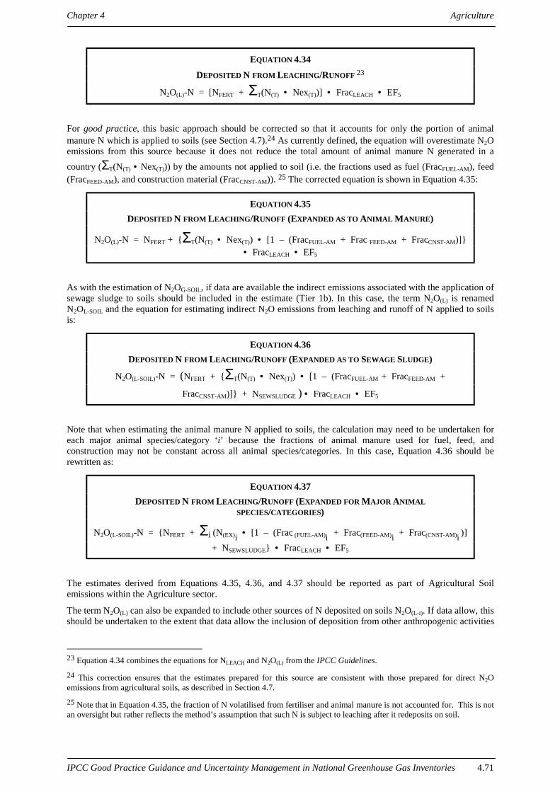
Chapter 4 Agriculture
IPCC Good Practice Guidance and Uncertainty Management in National Greenhouse Gas Inventories 4.71
EQUATION 4.34DEPOSITED N FROM LEACHING/RUNOFF 23
N2O(L)-N = [NFERT + ΣT(N(T) • Nex(T))] • FracLEACH • EF5
For good practice, this basic approach should be corrected so that it accounts for only the portion of animalmanure N which is applied to soils (see Section 4.7).24 As currently defined, the equation will overestimate N2Oemissions from this source because it does not reduce the total amount of animal manure N generated in a
country (ΣT(N(T) • Nex(T))) by the amounts not applied to soil (i.e. the fractions used as fuel (FracFUEL-AM), feed(FracFEED-AM), and construction material (FracCNST-AM)). 25 The corrected equation is shown in Equation 4.35:
EQUATION 4.35DEPOSITED N FROM LEACHING/RUNOFF (EXPANDED AS TO ANIMAL MANURE)
N2O(L)-N = NFERT + {ΣT(N(T) • Nex(T)) • [1 – (FracFUEL-AM + Frac FEED-AM + FracCNST-AM)]}• FracLEACH • EF5
As with the estimation of N2OG-SOIL, if data are available the indirect emissions associated with the application ofsewage sludge to soils should be included in the estimate (Tier 1b). In this case, the term N2O(L) is renamedN2OL-SOIL and the equation for estimating indirect N2O emissions from leaching and runoff of N applied to soilsis:
EQUATION 4.36DEPOSITED N FROM LEACHING/RUNOFF (EXPANDED AS TO SEWAGE SLUDGE)
N2O(L-SOIL)-N = (NFERT + {ΣT(N(T) • Nex(T)) • [1 – (FracFUEL-AM + FracFEED-AM +
FracCNST-AM)]} + NSEWSLUDGE ) • FracLEACH • EF5
Note that when estimating the animal manure N applied to soils, the calculation may need to be undertaken foreach major animal species/category ‘i’ because the fractions of animal manure used for fuel, feed, andconstruction may not be constant across all animal species/categories. In this case, Equation 4.36 should berewritten as:
EQUATION 4.37DEPOSITED N FROM LEACHING/RUNOFF (EXPANDED FOR MAJOR ANIMAL
SPECIES/CATEGORIES)
N2O(L-SOIL)-N = {NFERT + Σi (N(EX)i • [1 – (Frac (FUEL-AM)i + Frac(FEED-AM)i + Frac(CNST-AM)i )]+ NSEWSLUDGE} • FracLEACH • EF5
The estimates derived from Equations 4.35, 4.36, and 4.37 should be reported as part of Agricultural Soilemissions within the Agriculture sector.
The term N2O(L) can also be expanded to include other sources of N deposited on soils N2O(L-i). If data allow, thisshould be undertaken to the extent that data allow the inclusion of deposition from other anthropogenic activities
23 Equation 4.34 combines the equations for NLEACH and N2O(L) from the IPCC Guidelines.
24 This correction ensures that the estimates prepared for this source are consistent with those prepared for direct N2Oemissions from agricultural soils, as described in Section 4.7.
25 Note that in Equation 4.35, the fraction of N volatilised from fertiliser and animal manure is not accounted for. This is notan oversight but rather reflects the method’s assumption that such N is subject to leaching after it redeposits on soil.

Agriculture Chapter 4
IPCC Good Practice Guidance and Uncertainty Management in National Greenhouse Gas Inventories4.72
associated with agriculture that release NOx and NH3. This would include emissions of NOx and NH3 (in units ofN) from prescribed burning of savannas and field burning of agricultural residues.
Equation 4.38 shows the good practice approach for estimating N2O emissions from these additional indirectsub-source categories. For each source ‘i’ (i.e. prescribed burning of savannas and field burning of agriculturalresidues), the amount of N emitted as NOx and NH3 is multiplied by FracLEACH and EF5.
EQUATION 4.38DEPOSITED N FROM LEACHING/RUNOFF (EXPANDED AS TO ADDITIONAL INDIRECT SUB-
SOURCES)N2O(L-i)-N = (NOx-i + NH3-i) • FracLEACH • EF5
Although the method for estimating these additional sources of indirect emissions of N2O is presented here, theestimates should be reported under the source category in which the originating activity is reported.
Human consumption followed by municipal sewage treatment (N2O(S)): Human consumption of food resultsin the production of sewage, that can be processed in septic systems or wastewater treatment facilities, and thenmay seep into groundwater systems, be disposed of directly on land, or be discharged into a water source (e.g.rivers and estuaries). N2O can be produced during all of these processes through nitrification and denitrificationof sewage nitrogen. The IPCC Guidelines assume that N2O emissions associated with sewage treatment and landdisposal are negligible, so that all sewage nitrogen enters rivers and estuaries, where it is available fornitrification and denitrification. The method also recognises that some sewage N may be applied to soil assludge. To estimate total sewage nitrogen (NSEWAGE) using the method in the IPCC Guidelines, 26 the annual percapita protein consumption (PROTEIN, in kg protein/person-year) is multiplied by the national population(NrPEOPLE) and the fraction of protein that is nitrogen (FracNPR). NSEWAGE is then multiplied by the emission factorfor indirect emissions from sewage treatment (EF6) to obtain N2O emissions (in units of N) from discharge ofsewage (N2O(S)). The two equations presented in the IPCC Guidelines to calculate N2O emissions from dischargeof sewage are combined in the single good practice equation below:
EQUATION 4.39N2O EMISSIONS FROM DISCHARGE OF SEWAGE27
N2O(S)-N = PROTEIN • NrPEOPLE • FracNPR • EF6
It is good practice to use this basic approach, if a basic approach has also been used for estimating indirectemissions from the atmospheric deposition and leaching/runoff pathways (i.e. if Equations 4.31 and 4.35 havebeen used). If a more detailed estimate has been prepared for these other pathways, however, a more detailedapproach should also be used for this sub-category. To avoid double-counting of sewage N in this case, NSEWAGEshould be decreased by the amount of sewage N that is applied to soils in the form of sewage sludge(NSEWSLUDGE), and that has already been accounted for in estimating both N2O(G-SOIL) and N2O(L-SOIL). Therefore,the more detailed equation for estimating N2O(S), is :
EQUATION 4.40N2O EMISSIONS FROM DISCHARGE OF SEWAGE (EXPANDED AS TO SEWAGE SLUDGE)
N2O(S)-N = [(PROTEIN • NPEOPLE • FracNPR) – NSEWSLUDGE] • EF6
These emissions should be reported under Domestic and Commercial Wastewater in Chapter 5, Waste (Section5.2).
26 General guidance for estimating N2O emissions from human sewage is provided in Section 6.4, Nitrous Oxide fromHuman Sewage, IPCC Guidelines, Vol. 3. For a detailed description of the proposed method, the reader is referred to Section4.5.4 of the IPCC Guidelines, Reference Manual.
27 Equation 4.39 combines the equations for NSEWAGE and N2O(S) from the IPCC Guidelines.

Chapter 4 Agriculture
IPCC Good Practice Guidance and Uncertainty Management in National Greenhouse Gas Inventories 4.73
4.8.1.2 CHOICE OF EMISSION FACTORS
The method for estimating indirect N2O emissions includes three emission factors: one associated with depositednitrogen (EF4), the second associated with nitrogen lost through leaching and runoff (EF5), and the thirdassociated with nitrogen in discharged sewage (EF6).
Very little information exists, even on a global scale, for specifying EF4, EF5, and EF6. Therefore, although theIPCC Guidelines normally encourages inventory agencies to substitute country-specific data for default emissionfactors, for this source category the default values should be used unless rigorously documented and peer-reviewed country-specific values have been developed. The following discussion summarises the default valuesand describes some refinements of them. For good practice, the IPCC default emission factors are presented inTable 4.18, Default Emission Factors for Estimating Indirect N2O Emissions from N used in Agriculture.
• Emission factor for deposited nitrogen (EF4): The default value for EF4 is 0.01 kg N2O-N/kg NH4-N andNOx-N deposited. Country-specific values for EF4 should be used with great caution because of the specialcomplexity of transboundary atmospheric transport. Although inventory agencies may have specificmeasurements of N deposition and associated N2O flux, in many cases the deposited N may not haveoriginated in their country. Similarly, some of the N that volatilises in their country may be transported toand deposited in another country, where different conditions that affect the fraction emitted as N2O mayprevail.
• Emission factor for leaching and runoff (EF5): This value should be updated based on a recent re-examination of one of the factors from which it was derived. However, more research will be requiredbefore a new default value can be established.
• Emission factor for discharged sewage effluent: The default value for EF6 is 0.01 kg N2O-N/kg N. Thisvalue was derived by adding estimates of emission factors for rivers (EF5-r = 0.0075) and estuaries (EF5-e =0.0025). Country-specific values of EF6 must be used with great caution because of the complexity of thisemission pathway.
TABLE 4.18 DEFAULT EMISSION FACTORS FOR ESTIMATING INDIRECT N2O EMISSIONS FROM N USED IN AGRICULTURE
Emission Factor IPCC Default Value
EF4 (kg N2O-N/kg NH4-N & NOx-N deposited) 0.01
EF5 (kg N2O-N/kg N leached & runoff) 0.025
EF6 (kg N2O-N/kg sewage N discharged sewage effluent) 0.01
Source: IPCC Guidelines, Reference Manual, Table 4-23.
4.8.1.3 CHOICE OF ACTIVITY DATA
Much of the activity data required to estimate indirect N2O emissions, such as fertiliser consumption andlivestock nitrogen excretion, will have been previously developed for estimating emissions from other sourcecategories. Table 4.19, Data for Estimating Indirect N2O, summarises the key activity data required, anddescribes where to obtain them. It is essential that the same data sets be used across source categories to ensureconsistency in emission estimates.
As Table 4.19 shows, most of the activity data will be data developed for other source category estimates. Goodpractice in obtaining that data is described in the appropriate sections. The discussion below summarises goodpractice for developing the activity data:
• Estimating NOx and NH3 emissions from new source categories included for good practice: Emissionsof NOx and NH3 resulting from savanna burning and agricultural residue burning are required to estimateindirect N2O emissions from these activities. Estimation methods and default emission factors (or emissionratios) for estimating NOx emissions are included for these sub-categories in the IPCC Guidelines undertheir respective sectors or sub-sectors. The same methods used to estimate NOx emissions for each sub-category should be used to estimate NH3 emissions, but the NOx emission factors should be replaced withNH3 emission factors. A default emission factor of 0.038 Gg NH3-N/Gg fuel N (Crutzen and Andreae,

Agriculture Chapter 4
IPCC Good Practice Guidance and Uncertainty Management in National Greenhouse Gas Inventories4.74
1990)28 may be used to estimate NH3 emissions from savanna burning and agricultural residue burning ifcountry-specific emission factors are not available.
TABLE 4.19DATA FOR ESTIMATING INDIRECT N2O
Activity Data How to Obtain
NFERT From estimate of NFERT value collected for Direct N2O Emissions from Agricultural Soils
ΣT(N(T) • Nex(T)) From estimate of ΣT(N(T) • Nex(T)) value collected for Direct N2O Emissions from Agricultural Soils
NSEWSLUDGE From estimate of NSEWSLUDGE value collected for Direct N2O Emissions from Agricultural Soils
PROTEIN Food and Agricultural Organisation (FAO)
NrPEOPLE Food and Agricultural Organisation (FAO)
FracNPR See Table 4-24 in the IPCC Guidelines Reference Manual
FracLEACH See Table 4-24 in the IPCC Guidelines Reference Manual
FracGASF See Table 4-19 in the IPCC Guidelines Reference Manual
FracGASM See Table 4-19 in the IPCC Guidelines Reference Manual
FracFUEL-AM From estimate of FracFUEL-AM value collected for Direct N2O Emissions from Agricultural Soils
FracFEED-AM From estimate of FracFEED-AM value collected for Direct N2O Emissions from Agricultural Soils
FracCNST-AM From estimate of FracCNST-AM value collected for Direct N2O Emissions from Agricultural Soils
• Partitioning fractions for volatilisation (FracGASF, FracGASM): For the fraction of nitrogen that volatilisesas NH3 and NOx from applied synthetic fertilisers (FracGASF) and animal manure and sewage sludge(FracGASM), default values of 10% and 20%, respectively, are presented in the IPCC Guidelines. Country-specific volatilisation fractions can be used with reasonable documentation.
• Partitioning fraction for leaching (FracLEACH): A default value of 30% is presented in the IPCCGuidelines for FracLEACH. Note, however, that this default value was largely based on mass balance studiescomparing agricultural N inputs to N recovered in rivers. Agricultural practices (e.g. irrigation, frequentploughing, and drainage tiles) can promote heavy leaching losses of N applied to agricultural soils.However, for N that is deposited away from agricultural land, a lower value of FracLEACH may be moreappropriate. Future revisions of the method may reflect this consideration. Due to difficulties in developinga reliable factor for this source category, inventory agencies should use caution and provide rigorousdocumentation if using a country-specific factor.
• Partitioning fraction for nitrogen in protein (FracNPR): A default values of 16% is presented in the IPCCGuidelines for the fraction of animal and plant protein that is nitrogen (FracNPR). This term is not highlyvariable, and therefore country-specific values are unnecessary.
4.8.1.4 COMPLETENESS
Complete coverage for indirect N2O emissions from nitrogen used in agriculture requires estimation of emissions
from all of the agricultural input activities (i.e. NFERT, ΣT(N(T) • Nex(T)), and NSEWSLUDGE). If data are available,NSEWSLUDGE application (on all soils) can also be included. Complete coverage for indirect N2O emissions fromhuman sewage requires estimation of emissions from the discharge of sewage N (i.e. NSEWAGE, NSEWAGE minusNSEWSLUDGE).
28 Table 2 of Andreae and Crutzen (1990) is the basis for the NOx and NH3 emission factors associated with biomass
burning. Note that this table also lists an emission factor of 0.034 mole RCN per mole total N in biomass, on par with theNH3 emission factor. RCN is a form of nitrogen which is biologically available and therefore subject to microbialnitrification, denitrification, and N2O production. Furthermore, Table 2 of Andreae and Crutzen (1990) only accounts forabout 70% of biomass N, implying that combustion may yield additional, as yet unidentified forms of biologically availablenitrogen. Thus by only accounting for NOx and NH3 emissions, the method likely underestimates the total amount ofbiologically available nitrogen released by biomass burning.

Chapter 4 Agriculture
IPCC Good Practice Guidance and Uncertainty Management in National Greenhouse Gas Inventories 4.75
If data are available, the inventory should also include indirect N2O emissions from savanna burning andagricultural residue burning. These emissions are based upon direct emissions of NOx and NH3 from theseactivities.
4.8.1.5 DEVELOPING A CONSISTENT TIME SERIES
Emission estimates over a time series should be made using the same method (in terms of level of detail). Inter-annual changes in FracGASF, FracGASM, FracLEACH, FracNPR, EF4, EF5, and EF6 are not expected unless mitigationmeasures are undertaken. These factors should be changed only with the proper justification and documentation.If updated defaults for any of these variables become available through future research, inventory agencies mayrecalculate their historical emissions. For general good practice guidance on ensuring consistency in a timeseries, see Chapter 7, Methodological Choice and Recalculation, Section 7.3.2.2.
4.8.1.6 UNCERTAINTY ASSESSMENT
Information about emission factors (EF4, EF5, and EF6), leaching and volatilisation fractions are sparse andhighly variable. Expert judgement indicates that emission factor uncertainties are at least in order of magnitudeand volatilisation fractions of about +/−50%. Uncertainties in activity data estimates should be taken from thecorresponding direct emissions source categories. Chapter 6, Quantifying Uncertainties in Practice, providesadvice on quantifying uncertainties in practice including combining expert judgements and empirical data intooverall uncertainty estimates.
4 . 8 .2 R e p o r t in g a n d do c u me n t a t i onIt is good practice to document and archive all information required to produce the national emissions inventoryestimates as outlined in Chapter 8, Quality Assurance and Quality Control, Section 8.10.1, InternalDocumentation and Archiving. The worksheets in the IPCC Guidelines (Workbook) for calculating indirect N2Ofrom agricultural soils provide for transparent documentation of the default method of the IPCC Guidelines, andthe data used to implement the method. However, to implement good practice, these worksheets should beexpanded to incorporate the new variables that have been added to the deposition and leaching calculations (i.e.NSEWSLUDGE, FracFUEL-AM, FracFEED-AM, and FracCNST-AM) and should be revised to reflect Equations 4.31 and 4.35or 4.36.
The worksheets in the Workbook of the IPCC Guidelines used for calculating indirect N2O from human sewagealso provide for transparent documentation of the default method and the data used to implement the method.However, to implement the good practice approach, these worksheets must be expanded to incorporate the newvariable that has been added to the calculation (i.e. NSEWSLUDGE) and must be revised to reflect Equation 4.40.
To implement good practice for indirect N2O emissions from savanna burning and agricultural residue burning,new worksheets must be developed for each of these sub-categories. The worksheet for indirect N2O emissionsfrom savanna burning and agricultural residue burning should reflect Equations 4.33 and 4.38.
The reporting tables in the Reporting Instructions are inadequate. Direct and indirect agricultural N2O sourcesare reported together as one entry entitled ‘agricultural soils’ rather than separately. Furthermore, the title is amisnomer for indirect emissions, since a large fraction of these emissions occurs from aquatic systems. Toimprove the transparency of reporting, estimates of emissions from deposition and leaching should be reportedseparately. An explicit entry for indirect emissions from human sewage should be added in the Waste section.Entries for the new indirect N2O sources (savanna burning and agricultural residue burning) should also beadded to the reporting tables.
In addition to completing the reporting formats, the following additional information is necessary to documentindirect N2O emission estimates:
• Activity data: References for all activity data used in the calculations (i.e. complete citations for thestatistical database from which data were collected), and in cases when activity data were not availabledirectly from databases, the information and assumptions that were used to derive the activity data. Thisdocumentation should include the frequency of data collection and estimation, and estimates of accuracy andprecision.
• Emission factors: References for the emission factors that were used (specific IPCC default values orotherwise). In inventories in which country- or region-specific emission factors were used, or in which newmethods (other than the default IPCC methods) were used, the scientific basis of these emission factors or

Agriculture Chapter 4
IPCC Good Practice Guidance and Uncertainty Management in National Greenhouse Gas Inventories4.76
methods should be completely described and documented. This includes defining the input parameters anddescribing the process by which these emission factors or methods are derived, as well as describing sourcesand magnitudes of uncertainties.
• Emission results: Significant fluctuations in emissions between years should be explained. A distinctionshould be made between changes in activity levels and changes in emission factors from year to year and thereasons for these changes documented. If different emission factors are used for different years, the reasonsfor this should be explained and documented.
4 . 8 .3 I n v en t o ry q u a l i t y a s s u ra n c e /q u a l i ty c o n t r o l( Q A / Q C )
It is good practice to implement quality control checks as outlined in Chapter 8, Quality Assurance and QualityControl, Table 8.1, Tier 1 General Inventory Level QC Procedures, and expert review of the emission estimates.Additional quality control checks as outlined in Tier 2 procedures in Chapter 8, QA/QC, and quality assuranceprocedures may also be applicable, particularly if higher tier methods are used to determine emissions from thissource.
It is good practice to supplement the general QA/QC related to data processing, handling and reporting, asoutlined in Chapter 8, QA/QC, with source-specific procedures discussed below. The persons who collect dataare responsible for reviewing the data collection methods, checking the data to ensure that they are collected andaggregated or disaggregated correctly, and cross-checking the data with previous years to ensure that the data arereasonable. The basis for the estimates, whether statistical surveys or ‘desk estimates’ must be reviewed anddescribed as part of the QC effort. Documentation is a crucial component of the review process because itenables reviewers to identify mistakes and suggest improvements.
Review of emission factors• The inventory agency should review the parameters, equations and calculations used to develop the
emission factors. These QC steps are particularly important for subcategories in this source category becauseof the number of parameters that are used to construct the emission factors.
• If using country-specific factors, the inventory agency should compare them to the IPCC default factors.This is particularly important for the emission factors for deposited N and for discharged sewage, wherecaution should be used in developing country-specific factors.
Activ ity data check• Since many of the activity parameters used for this source category are also used for other agricultural
sources, it is critical to ensure that consistent values are being used.
• If using country-specific values for various parameters, (i.e. FracLEACH), the inventory agency shouldcompare them to the IPCC defaults. Rigorous documentation of the development of country-specific valuesshould also be maintained.
External review• Agricultural specialists (particularly nitrogen cycle specialists) as well as agricultural industry and other
stakeholders, should peer review the inventory estimates and all important parameters and emission factors.

Chapter 4 Agriculture
IPCC Good Practice Guidance and Uncertainty Management in National Greenhouse Gas Inventories 4.77
4 . 9 C H 4 E M I S S I O N S F R O M RI C EP R O D U C T I O N
4 . 9 .1 M e t h od o l og i c a l i s su e sAnaerobic decomposition of organic material in flooded rice fields produces methane (CH4), which escapes tothe atmosphere primarily by transport through the rice plants. The annual amount emitted from an area of riceacreage is a function of rice cultivar, number and duration of crops grown, soil type and temperature, watermanagement practices, and the use of fertilisers and other organic and inorganic amendments.
4.9.1.1 CHOICE OF METHOD
The IPCC Guidelines outline one method for estimating emissions from rice production, that uses annualharvested areas29 and area-based seasonally integrated emission factors.30 In its most simple form, the IPCCmethod can be implemented using national activity data (i.e. national total area harvested) and a single emissionfactor. However, the conditions under which rice is grown (e.g. water management practices, organic fertiliseruse, soil type) may be highly variable within a country, and these conditions can affect seasonal CH4 emissionssignificantly. The method can be modified to account for this variability in growing conditions by disaggregatingnational total harvested area into sub-units (e.g. harvested areas under different water management regimes), andmultiplying the harvested area for each sub-unit by an emission factor that is representative of the conditions thatdefine the sub-unit. With this disaggregated approach, total annual emissions are equal to the sum of emissionsfrom each sub-unit of harvested area. Thus, the basic equation is as follows:
EQUATION 4.41CH4 EMISSIONS FROM RICE PRODUCTION
Emissions from Rice Production (Tg/yr) = Σi Σj Σk (EFijk • Aijk • 10-12)
Where:
EFijk = a seasonally integrated emission factor for i, j, and k conditions, in g CH4/m2
Aijk = annual harvested area for i, j, and k conditions, in m2/yr
i, j, and k = represent different ecosystems, water management regimes, and other conditions underwhich CH4 emissions from rice may vary (e.g. addition of organic amendments)
The different conditions that should be considered include rice ecosystem type, water management regime, typeand amount of organic amendments, and soil type. The primary rice ecosystem types, and water managementregimes in each ecosystem type, are listed in Table 4.20, IPCC Default CH4 Emission Scaling Factors for RiceEcosystems and Water Management Regimes Relative to Continuously Flooded Fields. If rice is produced indistinct regions within the country (e.g. district, province), the equation above should be applied to each region.National emissions are equal to the sum of the regional estimates. In addition, if more than one crop is harvestedin a particular region during the year, and the conditions of cultivation (e.g. use of organic amendments) varyamong cropping seasons, then for that region, emissions should be estimated for each cropping season, and thensummed over all cropping seasons. In this case, the activity data are cultivated area, rather than harvested area.
If rice is a key source category (as defined in Chapter 7, Methodological Choice and Recalculation), inventoryagencies are encouraged to:
• Implement the IPCC method at the most disaggregated level possible;
29 In case of multiple cropping during the same year, ‘harvested area’ is equal to the sum of the area cultivated for eachcropping.
30 An emission factor represents the total missions over an entire cropping season (from land preparation until harvest or postseason drainage) per unit area. As in Appendix 4A.3, emission factors should be based on measurements over the entireperiod of flooding, and should account for fluxes of soil-entrapped methane that typically occur upon drainage.

Agriculture Chapter 4
IPCC Good Practice Guidance and Uncertainty Management in National Greenhouse Gas Inventories4.78
• Incorporate as many of the characteristics (i, j, k, etc.,) that influence CH4 emissions as possible;
• Develop country-specific emission factors to reflect the local impacts of these characteristics, preferablythrough collection of field data;
• Use emission factors and activity data at the same level of aggregation.
The decision tree in Figure 4.9, Decision Tree for CH4 Emissions from Rice Production, guides inventoryagencies through the process of applying the good practice IPCC approach. Implicit in this decision tree is ahierarchy of disaggregation in implementing the IPCC method. Within this hierarchy, the level of disaggregationutilised by an inventory agency will depend upon the availability of activity and emission factor data, as well asthe importance of rice as a contributor to national greenhouse gas emissions. The specific steps and variables inthis decision tree, and the logic behind it, are discussed in the text that follows the decision tree.
4.9.1.2 CHOICE OF EMISSION FACTORS
Ideally, inventory agencies will have seasonally integrated emission factors for each commonly occurring set ofrice production conditions in the country developed from standardised field measurements. These local,measurement-based emission factors account for the specific mix of different conditions that influence CH4emissions in one area implicitly. The most important conditions that influence rice emissions are summarised inBox 4.2:
BOX 4.2 CONSIDERATIONS FOR RICE PRODUCTION EMISSION FACTOR DEVELOPMENT
The following rice production characteristics should be considered in developing emission factors:
Regional differences in rice cropping practices: If the country is large and has distinct agriculturalregions, a separate set of measurements should be performed for each region.
Multiple crops: If more than one crop is harvested on a given area of land during the year, and thegrowing conditions vary among cropping seasons, emissions should be measured for each season.
Ecosystem type: At a minimum, separate measurements should be undertaken for each ecosystem(i.e. irrigated, rainfed, and deep water rice production).
Water management regime: Each ecosystem should be broken down further to account fordifferent water management practices (e.g. continuously flooded vs. intermittently flooded).
Addition of organic amendments: Measurements should be designed so that the effect of organicamendments (e.g. green manure, rice straw, animal manure, compost, weeds and other aquaticbiomass, etc.) on CH4 emissions can be quantified.
Soil type: Inventory agencies are encouraged to make every effort to undertake measurements onall major soil types under rice cultivation because of the significant influence that soil type canhave on CH4 emissions. Up to now the soil factor has not been taken into account in the IPCCGuidelines because data on harvested area by (major) soil type are not available from the standardactivity data sources. However, with the recent developments of models to simulate CH4 emissionsfrom rice fields, deriving scaling factors for major soil types grown to rice will be feasible in thenear future (e.g. Ding et al., 1996, and Huang et al., 1998). Combining measured or model-simulated soil type-specific scaling factors and a breakdown of rice acreage by soil type wouldfurther improve inventory accuracy if available.
Since some countries grow rice under a wide diversity of conditions, a complete set of local measurement-basedemission factors may not be possible. In this case, inventory agencies are encouraged to first obtain a seasonallyintegrated emission factor for continuously flooded fields without organic amendments (EFc), which is to beused as a starting point, and use scaling factors to adjust it to account for different conditions. The adjustedemission factors can then be determined using the following equation:

Chapter 4 Agriculture
IPCC Good Practice Guidance and Uncertainty Management in National Greenhouse Gas Inventories 4.79
F i g u r e 4 . 9 D e c i s i o n T r e e f o r C H 4 E m i s s i o n f r o m R i c e P r o d u c t i o n
Note 1: A key source category is one that is prioritised within the national inventory system because its estimate has a significantinfluence on a country’s total inventory of direct greenhouse gases in terms of the absolute level of emissions, the trend in emissions, orboth. (See Chapter 7, Methodological Choice and Recalculation, Section 7.2, Determining National Key Source Categories.)
Is there anyrice production in the
country?
Areharvested area data
available for all ecosystemsand waterregimes?
Arecountry-specific
seasonally integratedemission factors available
for each major ricecroppingregion?
Are theremultiple croppings
during the sameyear?
Areactivity data
available for the typeof water management practices,
type and amount of organicamendments and/or
soil type?
Report‘Not Occurring’
Collect data from theInternational Rice Research
Institute, or the Food andAgriculture Organization
Isrice production a
key source category?(Note 1)
Determine seasonally-integratedemission factors for each major rice
cropping region through a goodpractice measurement programme
Determine the appropriateemission factor for each cropping
(i.e. dry-, wet-, early-,single-, late-cropping)
Estimate emissionsfor each cropping in each
region using country-specific emission factors
Estimate emissions for each cropping ineach region, using country-specificemission factors and using scaling
factors for water management, organicamendments, and soil type
Estimate emissions usingdefault EF, and where data areavailable, using scaling factors
for organic amendmentsand other factors
Box 2
No
Yes
No
No
No
Yes
Yes
Yes
Box 3
Box 1
No
Yes
Yes
No

Agriculture Chapter 4
IPCC Good Practice Guidance and Uncertainty Management in National Greenhouse Gas Inventories4.80
EQUATION 4.42ADJUSTED SEASONALLY INTEGRATED EMISSION FACTOR
EFi = EFc • SFw • SFo • SFs
Where:
EFi = Adjusted seasonally integrated emission factor for a particular harvested area
EFc = Seasonally integrated emission factor for continuously flooded fields without organic amendments
SFw = Scaling factor to account for the differences in ecosystem and water management regime (fromTable 4.20)
SFo = Scaling factors should vary for both types and amount of amendment applied. (from Table 4.21,Dose-Response Table for Non-Fermented Organic Amendments)
SFs = Scaling factor for soil type, if available
The seasonally integrated emission factor for continuously flooded fields of major soil types without organicamendments should be determined through field measurements according to good practice procedures, asdiscussed in Appendix 4A.3. If data to determine EFc are not yet available, the IPCC default of 20 g/m2 may beused.
Scaling factors can be used to adjust the seasonally integrated emission factor for continuously flooded fields(EFc) to account for the various conditions discussed in Box 4.2. In order, the three most important scalingfactors are rice ecosystem/water management regime, organic amendments, and soil type. Country-specificscaling factors should only be used if they are based on well-researched and documented measurement data. Ifdata to determine scaling factors are not yet available, IPCC defaults can be used.
Water management system: The main types of methane-emitting rice ecosystems are irrigated, rainfed anddeep water. Within each ecosystem are water management systems, which affect the amount of CH4 emittedduring a cropping season. Table 4.20 provides IPCC default scaling factors for SFw that can be used whencountry-specific data are unavailable. Scaling factors for additional ecosystem types and water managementregimes can be applied only if country-specific data are available.
TABLE 4.20IPCC DEFAULT CH4 EMISSION SCALING FACTORS FOR RICE ECOSYSTEMS AND WATER MANAGEMENT REGIMES RELATIVE
TO CONTINUOUSLY FLOODED FIELDS (WITHOUT ORGANIC AMENDMENTS)
Category Water Management Regime Scaling Factor (SFw)Upland None 0
Continuous Flooded 1.0Intermittently Flooded – Single Aeration 0.5 (0.2-0.7)
Irrigated
Intermittently Flooded – MultipleAeration
0.2 (0.1-0.3)
Flood prone 0.8 (0.5-1.0)Rainfed
Drought prone 0.4 (0-0.5)
Water depth 50-100 cm 0.8 (0.6-1.0)
Lowland
Deep waterWater depth > 100 cm 0.6 (0.5-0.8)
Source: IPCC Guidelines, Reference Manual, Table 4-12.
Organic amendments: Good practice is to develop a scaling factor (SFo) that incorporates information on thetype and amount of organic amendment applied (rice straw, animal manure, green manure, compost, andagricultural wastes). On an equal mass basis, more CH4 is emitted from amendments containing higher amountsof easily decomposable carbon, and emissions also increase as more of each organic amendment is applied.Table 4.21 presents an approach to vary the scaling factor according to the amount of amendment applied.
Theoretically, the different amendments should be ranked according to the carbon content per unit of weight, butmost often only information on the amount applied is available. In this case, the inventory agency shoulddistinguish between fermented and non-fermented organic amendments. CH4 emissions from fermentedamendments (e.g. compost, residue of biogas pits) are significantly lower than non-fermented amendments

Chapter 4 Agriculture
IPCC Good Practice Guidance and Uncertainty Management in National Greenhouse Gas Inventories 4.81
because they contain much less easily decomposable carbon. Denier van der Gon and Neue (1995) empiricallydetermined a reduction factor of six implying that the increase in CH4 emission upon application of 12 t/hacompost is comparable to the increase upon application of 2 t/ha non-fermented organic amendment.
TABLE 4.21
DOSE-RESPONSE TABLE FOR NON-FERMENTED ORGANIC AMENDMENTS
Amount applied as dry matter(t/ha)
Scaling factor (SFo)
Range
1-2 1.5 1-2
2-4 1.8 1.5-2.5
4-8 2.5 1.5-3.5
8-15 3.5 2-4.5
15+ 4 3-5
Note: To use the table for fermented organic amendments, divide the amount applied by six.Source: Derived from Denier van der Gon and Neue, 1995.
Soil types: In some cases emission data for different soil types are available and can be used to derive SFs. Themajor motivation to incorporate soil type as a scaling factor is that both experiments and mechanistic knowledgeconfirm its importance. It is anticipated that in the near future simulation models will be capable of producingsoil-specific scaling factors.
4.9.1.3 CHOICE OF ACTIVITY DATA
Activity data consist of rice production and harvested area statistics, which should be available from a nationalstatistics agency. The activity data should be broken down by rice ecosystem or water management type. If thesedata are not available in-country, they can be downloaded from an FAO website:(http://www.fao.org/ag/agp/agpc/doc) or can be obtained from IRRI's World Rice Statistics (e.g. IRRI, 1995).Most likely, the accuracy of activity data will be high compared to the accuracy of the emission factor. However,for various reasons the area statistics may be biased and a check of the harvested area statistics for (parts of) thecountry with remotely sensed data is encouraged.
In addition to the essential activity data requested above, it is good practice to match data on organicamendments and soil types to the same level of disaggregation as the activity data. It may be necessary tocomplete a survey of cropping practices to obtain data on the type and amount of organic amendments applied.
4.9.1.4 COMPLETENESS
Complete coverage for this source category requires estimation of emissions from the following activities, wherepresent:
• If soil submergence is not limited to the actual rice growing season, emissions outside of the rice growingseason should be included (e.g. from a flooded fallow period);
• Other rice ecosystem categories, like swamp, inland-saline or tidal rice fields may be discriminated withineach sub-category according to local emission measurements;
• If more than one rice crop is grown annually, these rice crops should be reported independently according tothe local definition (e.g. early rice, late rice, wet season rice, dry season rice). The rice crops may fall intodifferent categories with a different seasonally integrated emission factor and different correction factors forother modifiers like organic amendments.
4.9.1.5 DEVELOPING A CONSISTENT TIME SERIES
The emission estimation method should be applied consistently to every year in the time series, at the same levelof disaggregation. If detailed activity level data are unavailable for earlier years, emissions for these years shouldbe re-calculated according to the guidance provided in Chapter 7, Methodological Choice and Recalculation,Section 7.3. If there have been significant changes in agricultural practices affecting CH4 emissions over the

Agriculture Chapter 4
IPCC Good Practice Guidance and Uncertainty Management in National Greenhouse Gas Inventories4.82
times series, the rice estimation method should be implemented at a level of disaggregation which is sufficient todiscern the effects of these changes. For example, various trends in (Asian) rice agriculture such as the adoptionof new rice varieties, increasing use of inorganic fertiliser, improved water management, changing use of organicamendments, and direct seeding may lead to increases or decreases in overall emissions. To weigh the impact ofthese changes, it may be necessary to use model studies.
4.9.1.6 UNCERTAINTY ASSESSMENT
Table 4.22 presents a default emission factor, default scaling factors, and ranges for the default values. The rangeof emission factor, defined as the standard deviation about the mean, indicates the uncertainty associated withthis default value for this source category. The uncertainty may be influenced by the following:
Natural Variability: The natural variability is a result of variations in natural controlling variables, such asannual climate variability, and variability within units that are assumed to be homogenous, such as spatialvariability in a field or soil unit. For this source category, good practice should permit determination ofuncertainties using standard statistical methods when enough experimental data are available. Studies to quantifysome of this uncertainty are rare but available (e.g. for soil type induced variability). The variability found insuch studies is assumed to be generally valid. For more detail, see Sass (1999).
Lack of activity data and documentation: Important activity data necessary to apply scaling factors (i.e. dataon cultural practices and organic amendments) may not be available in current databases/statistics. Estimates ofthe fraction of rice farmers using a particular practice or amendment must then be based on expert judgement,and the range in the estimated fraction should also be based on expert judgement. As a default value for theuncertainty in the fraction estimate, ± 0.2 is proposed (e.g. the fraction of farmers using organic amendmentestimated at 0.4, the uncertainty range being 0.2-0.6). Chapter 6, Quantifying Uncertainties in Practice, providesadvice on quantifying uncertainties in practice including combining expert judgements and empirical data intooverall uncertainty estimates.
TABLE 4.22DEFAULT EMISSION FACTOR, DEFAULT SCALING FACTORS, AND RANGES FOR CH4 EMISSIONS FROM RICE FIELD
Emission component Default value Ranges
Standard emission factor (EF) 20 g CH4 m-2 season-1 12-28 g CH4 m-2 season-1
Scaling factor water management SFw See Table 4.20 Table 4.20Scaling factor organic amendments SFo 2 1.5-5Scaling factor soil types SFs 1 0.1-2Source: IPCC Guidelines and Judgement by Expert Group (see Co-chairs, Editors and Experts; CH4 Emissions from Rice Production).
4 . 9 .2 R e p o r t in g a n d do c u me n t a t i onIt is good practice to document and archive all information required to produce the national emissions inventoryestimates as outlined in Chapter 8, Quality Assurance and Quality Control, Section 8.10.1, InternalDocumentation and Archiving. It is good practice to document the emission estimate by reporting theinformation required to fill out the rice worksheet in the Workbook of the IPCC Guidelines. Inventory agenciesthat do not use the worksheets should provide comparable information. If the emission estimate is disaggregatedby region, information on each region should be reported.
The following additional information should be reported, if available, to ensure transparency:
• Water management practices;
• The types and amounts of organic amendments used. (Incorporation of rice straw or residues of the previous(non-rice) crop should be considered an organic amendment, although it may be a normal productionpractice and not aimed at increasing nutrient levels as is the case with manure additions);
• Soil types used for rice agriculture;
• Number of rice crops grown annually;
• Most important rice cultivars grown.

Chapter 4 Agriculture
IPCC Good Practice Guidance and Uncertainty Management in National Greenhouse Gas Inventories 4.83
When simple default emission factors are used to estimate CH4 emissions, uncertainty can increase dramatically.Inventory agencies using country-specific emission factors should provide information on the origin and basis ofthe factor, compare it to other published emission factors, explain any significant differences, and attempt toplace bounds on the uncertainty.
4 . 9 .3 I n v en t o ry q u a l i t y a s s e s s me n t / q u a l i ty c o n t r o l( Q A / Q C )
It is good practice to implement quality control checks as outlined in Chapter 8, Quality Assurance and QualityControl, Table 8.1, Tier 1 General Inventory Level QC Procedures, and expert review of the emission estimates.Additional quality control checks as outlined in Tier 2 procedures in Chapter 8, QA/QC, and quality assuranceprocedures may also be applicable, particularly if higher tier methods are used to determine emissions from thissource.
A detailed treatment on inventory QA/QC for field measurement is given by Sass (1999) and in Appendix 4A.3.Some important issues are highlighted and summarised below.
Compiling national emissions: It is, at present, not possible to cross-check emissions estimates from this sourcecategory through external measurements. However, the inventory agency should ensure that emission estimatesundergo quality control by:
• Cross-referencing aggregated crop yield and reported field area statistics with national totals or othersources of crop yield/area data;
• Back-calculating national emission factors from aggregated emissions and other data;
• Cross-referencing reported national totals with default values and data from other countries.

Agriculture Chapter 4
IPCC Good Practice Guidance and Uncertainty Management in National Greenhouse Gas Inventories4.84
A P P E N D I X 4 A . 1C H 4 A N D N 2 O E M I S SI O N S F R O M S A V A N N AB U R N I N G : B A SI S F O R F U T U R EM E T H O D O L O G I C A L D E V E L OP M E NT
4 A . 1 .1 M e t h o d o l o g i c a l i s s u e sIn savanna regions burning is carried out every one to several years. The burning results in instantaneousemissions of carbon dioxide (CO2). As the vegetation regenerates between burning cycles, however, the CO2released into the atmosphere is reabsorbed during the next vegetation growth period. For this reason, net CO2emissions from savanna burning are assumed to be zero. Savanna burning also releases other trace gases,including CH4, CO, NMVOCs, N2O and NOx. In this chapter, only emissions of the direct greenhouse gases CH4and N2O are discussed.
4A.1.1.1 CHOICE OF METHOD
The choice of method depends upon the availability of activity data and emission factors for CH4 and N2O. If aninventory agency does not have activity data and emission factors, the default values in the IPCC Guidelinesmay be used.
The current method requires a value for the living fraction of aboveground biomass in Table 4-12 of theWorkbook of the IPCC Guidelines. In addition, Table 4-13 of the IPCC Guidelines requires values for oxidisedfraction and carbon fraction in living and dead biomass for calculating the amount of carbon and nitrogenreleased from savanna burning. These parameters are difficult to measure in the field. Combustion efficiency canbe used to depict the vegetation and combustion conditions, which ultimately determine the emission factors ofCH4 and N2O. The combustion efficiency is defined as the molar ratio of emitted CO2 concentrations to the sumof emitted CO and CO2 concentrations from savanna fires. A column for combustion efficiency is included inTable 4.A1 of this document. The compiled combustion efficiency data are derived from the results of biomassburning experiments in different savanna ecosystems in tropical America and Africa. Therefore, in the proposedmethod the revised equation for computing the amount of CH4 or N2O emitted per year would be:
EQUATION 4.A1CH4 OR N2O RELEASED FROM SAVANNA BURNING
Amount of CH4 or N2O released = Amount of biomass burned (t dm) • Emission factor of CH4or N2O (kg/t dm)

Chapter 4 Agriculture
IPCC Good Practice Guidance and Uncertainty Management in National Greenhouse Gas Inventories 4.85
TABLE 4.A1
AMOUNT OF ABOVEGROUND BIOMASS BURNED
Region Fraction of TotalSavanna Burned
Annually
AbovegroundBiomass Density
(t dm/ha)
Fraction of BiomassActually Burned
CombustionEfficiency
Tropical America
Campo limpoa.b
Campo sujoa.b
Campo cerradoa.b
Cerrado sensu strictoa.b
0.50
0.3-1.0
0.3-1.0
0.3-1.0
0.3-1.0
6.6±1.8
7.1±0.5
7.3±0.5
8.6±0.8
10.0±0.5
0.85
1.0
0.97
0.72
0.84
0.95
0.96
0.94
0.94
Tropical Africa
Sahel zone
North Sudan zone
South Sudan zone
Guinea zone
Moist Miomboc.d,e
Semiarid Miomboc,e
Moist Damboc,d,e
Fallow Chitemenec,e
Semiarid Woodland
(South Africa) c,e
0.75
0.05-0.15
0.25-0.50
0.25-0.50
0.60-0.80
0.5-1.0
0.5-1.0
0.5-1.0
0.1
0.25-0.5
6.6±1.6
0.5-2.5
2-4
3-6
4-8
8.9±2.7
5.1±0.4
3.0±0.5
7.3±0.7
4.6±2.8
0.86
0.95
0.85
0.85
0.90-1.0
0.74±0.04
0.88±0.02
0.99±0.01
0.71±0.05
0.85±0.11
0.94
0.92
0.91
0.95
0.96
0.93
aKauffman et al. (1994), bWard et al. (1992), cShea et al. (1996), dHoffa et al.(1999), eWard et al. (1996).
For regions not specifically listed, data are contained in Table 4-14 of the IPCC Guidelines, Reference Manual(same as Table 4-12 of the Workbook of the IPCC Guidelines.) This table provides the basic ecological zonesaccording to the available savanna statistics. Table 4.A1 above contains additional savanna data for fourecological zones in tropical America and five ecological zones in tropical Africa, based on the results of fieldexperiments in Brazil, Zambia, and South Africa.
If an inventory agency has the necessary data for the fraction of savanna area burned annually, the abovegroundbiomass density, and the fraction of biomass actually burned in each ecological zone, the amount of biomassburned can be calculated at a disaggregated level.
It is desirable to develop the seasonal-dependent activity data and the emission factors of CH4 and N2O fromsavanna burning in various savanna ecosystems in each country if data are available. Fewer savanna areas and asmaller percentage of aboveground biomass are burned in the early dry season than in the late dry season.Therefore, as the dry season progresses in different savanna ecosystems, it is critical to monitor (i) the fraction ofburned savanna area; (ii) the aboveground biomass density; (iii) the percentage of the aboveground biomassburned; and (iv) combustion efficiency.
4A.1.1.2 CHOICE OF EMISSION FACTORS
For savanna fires, there is a linear negative correlation between the CH4 emission factor and the combustionefficiency. The emission factor is high for a fire of low combustion efficiency. The relationship is similarregardless of the climatic zone, the herbaceous species, or the amount of aboveground biomass.
Table 4.A2 lists different combustion efficiencies and associated CH4 emission factors. Once the combustionefficiency of a savanna fire is determined according to the ecological zone and the burning period, the

Agriculture Chapter 4
IPCC Good Practice Guidance and Uncertainty Management in National Greenhouse Gas Inventories4.86
corresponding emission CH4 factor should be used to calculate the amount of CH4 released per year fromsavanna burning.
TABLE 4.A2
COMBUSTION EFFICIENCY AND CORRESPONDINGCH4 EMISSION FACTOR
Combustion Efficiency CH4 Emission Factor (kg/t dm)
0.88 4.2
0.90 3.4
0.91 3.0
0.92 2.6
0.93 2.3
0.94 1.9
0.95 1.5
0.96 1.1
Source: Ward et al. (1996).
The emission of N2O from biomass burning is linearly correlated with the emission of CO2 and is dependent onthe nitrogen content of the vegetation. The emission factor of N2O is calculated by the equation:
EQUATION 4.A2N2O EMISSION FACTOR
Emission factor of N2O (kg/t dm) = Emission factor of CO2 (kg/t dm) • 1/Molecular weight ofCO2 • Molar emission ratio of N2O to CO2 • Molecular weight of N2O
Equation 4.A2 is simplified to:
EQUATION 4.A3N2O EMISSION FACTOR
Emission factor of N2O (kg/t dm) = Emission factor of CO2 (kg/t dm) • Molar emission ratio ofN2O to CO2
Since N2O is not stable during storage of smoke samples, the molar emission ratio of N2O to CO2 has beenderived from laboratory experiments in which different types of vegetation were burned (Hao et al., 1991) andcan be expressed by:
EQUATION 4.A4MOLAR EMISSION RATIO OF N2O TO CO2
Molar emission ratio of N2O to CO2 = 1.2 • 10-5 + [3.3 • 10-5 • Molar ratio of nitrogen tocarbon (N/C) in the biomass]
Emission factors for N2O in several savanna ecosystems have been tabulated in Table 4.A3 on the basis of theresults of field measurements of CO2 emissions and the N/C ratios of the biomass. The default emission factorsfor N2O in tropical America and Africa are calculated by averaging the emission factors for the continent. If aninventory agency has data on the N/C ratio in the biomass and assumes the emission factor for CO2 to be 1700kg/t dm, the emission factor for N2O can be calculated by the two Equations 4.A3 and 4.A4 above.

Chapter 4 Agriculture
IPCC Good Practice Guidance and Uncertainty Management in National Greenhouse Gas Inventories 4.87
TABLE 4.A3
EMISSION FACTORS OF N2O IN VARIOUS SAVANNA ECOSYSTEMS
Region Emission Factor of CO2(kg/t dm)
N/C Ratio in Biomass(%)
Emission Factor of N2O(kg/t dm)
Tropical AmericaCampo limpoa, b, c
Campo sujoa, b, c
Campo cerradoa, b, c
Cerrado sensu strictoa, b, c
-1745170016981722
-0.600.560.951.02
0.0650.0550.0520.0740.079
Tropical AfricaMoist Miombob, c, d
Semiarid Miombob, c, d
Moist Dambob, c, d
Fallow Chitemeneb, c, d
Semiarid Woodland
-16801649173217611699
-1.420.940.330.77
0.98 ± 0.11
0.0700.0990.0710.0400.0660.075
Source: aWard et al. (1992), bSusott et al. (1996), cHao et al. (1991), dWard et al. (1996).
4A.1.1.3 CHOICE OF ACTIVITY DATA
The activity statistics for each savanna ecosystem include the following values: the savanna area; the fraction ofsavanna area burned; the aboveground biomass density; the fraction of aboveground biomass burned; and thecarbon and nitrogen content in the biomass. Other parameters (i.e. the fraction of living and dead biomass burnedand the carbon/nitrogen fraction of living and dead biomass) have been removed here because of thecomplexities of collecting these data in the field. Since the emission factor for CH4 can decrease by 50-75% asthe burning season progresses, it is strongly suggested that each inventory agency collect seasonal data on thefraction of savanna area burned, the aboveground biomass density, and the fraction of aboveground biomassburned in each savanna ecosystem from the early dry season to the late dry season.
4A.1.1.4 DEVELOPING A CONSISTENT TIME SERIES
Since there is a large degree of uncertainty in determining the burned area in each savanna ecosystem, it may beuseful to take an average of at least three years to provide a base year estimate for identification of any trend inthe emissions of CH4 and N2O from savanna burning. The methods for ensuring a consistent time series aredescribed in Chapter 7, Methodological Choice and Recalculation.
4A.1.1.5 UNCERTAINTY ASSESSMENT
The uncertainty of the emission factor for CH4 is about ±20%, based on the results of extensive field experimentsin tropical America and Africa. The uncertainty of the N2O emission factor is also about ±20%, based onextensive laboratory experiments. The uncertainty of the aboveground biomass density in a savanna ecosystemranges from ±2% to ±60%. The larger uncertainty is probably due to the variation of the composition ofaboveground biomass at different sites. The uncertainty of the fraction of biomass actually burned is less than±10%. Presently, it is difficult to estimate the uncertainty for the fraction of savanna area burned each year, orthe amount of burning in, for example, the early and late season.
4 A . 1 .2 R e p o r t in g a n d do c u me n t a t i o nIt is good practice to document and archive all information required to produce the national emissions inventoryestimates as outlined in Chapter 8, Quality Assurance and Quality Control, Section 8.10.1, InternalDocumentation and Archiving. The reporting in the worksheets contained in the IPCC Guidelines is transparent,however, the most critical issue in reporting and documentation is that majority of the activity data (e.g. thepercentage of savanna area burned, the aboveground biomass density, and the fraction of biomass actually

Agriculture Chapter 4
IPCC Good Practice Guidance and Uncertainty Management in National Greenhouse Gas Inventories4.88
burned) are not available or are difficult to collect in the field. There are also no standard methods of collectingthe information on area burned and fraction of biomass actually burned, resulting in inconsistency among thereported data.
4 A . 1 .3 I n v en t o ry q u a l i t y a s s u ra n c e /q u a l i ty c on t r o l( Q A / Q C )
As mentioned above, there are large degrees of uncertainty in the activity data to compute the amount of biomassburned in savanna. Very limited data are available on the seasonal trends of the savanna areas burned, theaboveground biomass densities, and the fractions of aboveground biomass burned. The monitoring of thelocations of active savanna fires and the mapping of burned areas in each country can be improved by using thesatellite imagery available from various national and international agencies. In addition, standard methods haveto be developed to measure the aboveground biomass density, the fraction of biomass burned, and thecombustion efficiency in order to ensure the quality and consistency of the data.

Chapter 4 Agriculture
IPCC Good Practice Guidance and Uncertainty Management in National Greenhouse Gas Inventories 4.89
A P P E N D I X 4 A . 2C H 4 A N D N 2 O E MI S SI ONS FROMA G R I C U L T U R A L R E SI D U E B U R NI N G : B A SI SF O R F U T U R E M ET H O D O L O G I C A LD E V E L OP ME N TAlthough the burning of agricultural residues is not considered a net source of carbon dioxide because the carbonreleased to the atmosphere is reabsorbed during the next growing season, this burning is a source of netemissions of many trace gases including CH4, CO2, N2O, and NOx. It is important to note that some agriculturalresidues are removed from the fields and burned as a source of energy, especially in developing countries. Non-CO2 emissions from this type of burning are dealt with in the Energy sector of the IPCC Guidelines. Cropresidue burning must be properly allocated to these two components in order to avoid double counting. Thefollowing discussions are focused only on the direct greenhouse gases CH4 and N2O.
4 A . 2 .1 M e t h o d o l o g i c a l i s s u e s
4A.2.1.1 CHOICE OF METHOD
The choice of method will depend on the availability of activity data and emission factors for CH4 and N2O ineach country. Where available, country-specific activity data and emission factors for CH4 and N2O should beused. If a country does not have its own activity data and emission factors, the default values in the IPCCGuidelines may be used instead.
The largest degree of uncertainty in estimating the emission inventories of CH4 and N2O from agriculturalresidue burning is the fraction of agricultural residue burned in the field. The percentage of residue burned on-site must be based on a complete mass balance accounting of the residue. For substantial improvement in theemission estimates of CH4 and N2O, inventory agencies are encouraged to estimate local and regional practicesthat reflect: (i) the fraction of residue burned in the field; (ii) the fraction transported off the field and burnedelsewhere (associated with processing); (iii) the fraction consumed by animals in the field; (iv) the fractiondecayed in the field; and (v) the fraction used by other sectors (e.g. biofuel, domestic livestock feed, buildingmaterials, etc.). Currently, it is estimated that 10% of the total agricultural residue is burned in the field indeveloped countries and 25% in developing countries. These figures may be too high. Good practice suggeststhat an estimate of 10% may be more appropriate for developing countries.
4A.2.1.2 CHOICE OF EMISSION FACTORS
The CH4 and N2O emission factors in Table 4.16 of the Workbook of the IPCC Guidelines are generallyreasonable. There are also insufficient data to update these emission factors as few field experiments have beenconducted in the past five years that measure emissions produced by burning agricultural residue in the field.Emission factors, however, are probably dependent on weather conditions in the burning periods, as the emissionfactor of CH4 from savanna burning decreases from the early dry season to the late dry season. If an inventoryagency is conducting experiments to measure the CH4 and N2O emission factors from burning agriculturalresidue, the experiments should be carried out in the dry season and rainy season when crop residue is burned.
4A.2.1.3 CHOICE OF ACTIVITY DATA
The activity data for crop production can be obtained from either the country’s data or the FAO ProductionYearbook (U.N. Food and Agriculture Organisation). These statistical data are reasonably accurate. There arefew data available to update residue/crop ratios, dry matter fractions, carbon fractions, and nitrogen to carbonratios for different crop residue. When an inventory agency is compiling its activity data, it is necessary tocollect monthly weather data and data on the amount of each crop residue burned after harvest. Weatherconditions would influence the combustion efficiency (see Appendix 4A.1 of this chapter) and the CH4 and N2Oemission factors.

Agriculture Chapter 4
IPCC Good Practice Guidance and Uncertainty Management in National Greenhouse Gas Inventories4.90
4A.2.1.4 COMPLETENESS
The current method incorporates all the factors necessary to estimate the CH4 and N2O emissions from burningagricultural residue. Several crops are missing in Table 4.15 of the Workbook of the IPCC Guidelines (e.g.sugarcane and root crops such as cassava and yam). The ratio of residue to crop is 0.16 for sugarcane and 0.4 forroot crops. It is important to account for the entire disposition of agricultural residue in the mass balance.Residue not being burned in the field will become a source of CH4 or N2O from microbial decomposition,domestic energy consumption, and domestic waste. These sources will have to be incorporated into thecomputation of CH4 and N2O emissions from other activities.
4A.2.1.5 DEVELOPING A CONSISTENT TIME SERIES
There are good prospects for developing the trend of CH4 and N2O emissions from agricultural residue burningbecause the statistics of agricultural production are compiled with reasonable accuracy. The weakness in thecomputation is estimating the percentage of residue burned in the field. Each inventory agency has to collectactivity data on disposition of each crop residue, especially the percentage of residue burned on-site, afterharvest.
4A.2.1.6 UNCERTAINTY ASSESSMENT
Crop production data, including cash crops and subsistence farming, are reasonably accurate, although it isdifficult to determine the uncertainty. The uncertainties in CH4 and N2O emission factors for burning agriculturalresidue in the dry season are about ±20%. It is not known, however, about the emission factors in the rainyseason. The fraction of agricultural residue burned in the field is probably the variable with the largest degree ofuncertainty in estimating the amount of CH4 and N2O emitted from agricultural residue burning. Statistical datahave to be compiled to account for the use of agricultural residue after harvest.
4 A . 2 .2 R e p o r t in g a n d do c u me n t a t i o nIt is good practice to document and archive all information required to produce the national emissions inventoryestimates as outlined in Chapter 8, Quality Assurance and Quality Control, Section 8.10.1, InternalDocumentation and Archiving. Agricultural production data are easily accessible from each country or the FAOProduction Yearbook. Weather conditions and the amount of each crop burned in the field during the dry seasonand rainy season have to be reported. It is necessary to measure and report the dry matter fraction, the carbonfraction, and the nitrogen to carbon ratio for each crop residue. It is also important to conduct field experimentsthat measure the CH4 and N2O emission factors in the dry and rainy season.
4 A . 2 .3 I n v en t o ry q u a l i t y a s s u ra n c e /q u a l i ty c on t r o l( Q A / Q C )
The quality of CH4 and N2O emissions estimates from agricultural residue burning will vary considerably fromcountry to country, depending largely on the quality of the data on the percentage of the residue burned in thefield. The qualities of other activity data and emission factors are reasonable and can be improved by collectingthe data of the amount of residue burned during the dry season and rainy season. Crop production data can beverified by using commodity trade statistics.
Chapter 4 Agriculture
IPCC Good Practice Guidance and Uncertainty Management in National Greenhouse Gas Inventories 4.91
A P P E N D I X 4 A . 3C H 4 E M I S S I O N S F R O M RI C E P R O D U C T I O N :M E A S U RE M E NT , R E P O R T I N G , A N D Q A / Q C O FF I E L D D AT AConducting Field Measurement: A standardised control rice plot with at least three replicate fields should beused to obtain standard regional and country emission factors. Plots are to be kept flooded from shortly beforetransplanting until maturity. The experimental plots should not have a recent history (i.e. five years) of addedorganic amendments to the soil other than recycled roots and perhaps short stubble. CH4 flux measurementsshould be recorded at least twice per week over an entire flooded season. In areas where double or triple ricecropping is practised, data should be collected for all growing seasons. For a guideline for good practicestandardised measurements for the irrigated rice ecosystem, see IGAC (1994). The nature of the instrumentationand the frequency of measurement will determine the associated uncertainty. For typical measurements, theassociated uncertainty is expected to be at least 20%.
The accuracy and precision of CH4 emission estimates increases with both the number of sites tested and thefrequency and number of measurements at each site.
Other data, such as the location and extent of area that the measurement represents, soil data, and climateinformation, should be collected. Agronomic data such as rice yield and other crop production data are alsoimportant because these data can be used to determine if measurements are representative of typical agronomicconditions. In general, the various predictive models that have been recently published (e.g. Huang et al., 1998)may aid in reporting CH4 emission values. Good practice is to provide as much country- or region-specific detailas is feasible.
Reporting of Field Measurements: The minimum data set that should accompany flux measurements for (i)scaling factor determination, (ii) verification of inventory using models and, (iii) QA/QC consists of:
• Geographic data including site country and province, latitude and longitude, average elevation, and a shortdescription of the location;
• A data log of agricultural events (e.g. time of organic input application, water management, weeding, etc.),method of crop establishment and dates of important plant events (e.g. transplanting, heading, harvest date);
• Air and soil temperature at 5 cm depth taken at the time of each flux measurement;
• Fertiliser types, application rates (including chemical amendments), and timing and mode of application;
• Soil types classified according to USDA Soil Taxonomy or FAO/UNESCO Soil Classification, at least onsubgroup levels. General soil characteristics, including texture, should be measured;
• Water management (number of flooding days, drainage/drought events);
• Impact of organic amendment on emissions (type and amount of amendment should be documented);
• Rice cultivar used (name, crop duration, height, traditional or modern variety, specific traits);
• Plant parameters preferably for different growth stages (e.g. leaf area index, above ground biomass (strawand stubble), yield, harvest index).
Field Measurement QA/QC: Country scientists will usually determine field-level QA/QC procedures toestablish country-specific emission factors. To ensure the comparability and inter-calibration of extended datasets used to establish country-specific emission factors, there are certain internationally determined procedures toobtain ‘standard emission factors’ that should be common to all monitoring programs (see IGAC (1994), Sass(1999)):
(i) CH4 flux measurements should be recorded at least twice per week over an entire flooded season.
(ii) In areas where double rice cropping (or 5 rice crops in 2 years) is practised, data should be collected forall growing seasons.
(iii) Manual sampling of flux chambers may miss the large fluxes of soil-entrapped CH4 upon drainage. Insuch cases, a correction should be made. If no specific data are available, an estimated 10-20% increaseof seasonal emission can be applied.
(iv) Significance of pre-planting emissions should be discussed and, if appropriate, estimated or measured.

Agriculture Chapter 4
IPCC Good Practice Guidance and Uncertainty Management in National Greenhouse Gas Inventories4.92
R E F E R E N CE S
LIVESTOCK POPULATION CHARACTERISATIONAgricultural and Food Research Council (AFRC) Technical Committee on Responses to Nutrients (1993)
Energy and Protein Requirements of Ruminants. 24-159, CAB International, Wallingford, U.K.
AFRC Technical Committee on Responses to Nutrients (1990) Nutritive Requirements of Ruminant Animals:Energy. Rep. 5, CAB International, Wallingford, U.K.
Bamualim, A. and Kartiarso (1985) ‘Nutrition of draught animals with special reference to Indonesia.’ In:Draught Animal Power for Production. J.W. Copland (ed.). Australian Centre for International agriculturalResearch (ACIAR), Proceedings Series No. 10. ACIAR, Canberra, A.C.T., Australia.
Food and Agriculture Organisation (FAO) (1999) Statistical Database.
Ibrahim, M.N.M. (1985) ‘Nutritional status of draught animals in Sri Lanka.’ In: Draught Animal Power forProduction, J.W. Copland (ed.). ACIAR (Australian Centre for International Agricultural Research)Proceedings Series No. 10. ACIAR, Canberra, A.C.T., Australia.
Intergovernmental Panel on Climate Change (IPCC) (1997) Revised 1996 IPCC Guidelines for NationalGreenhouse Gas Inventories, J.T. Houghton et al., IPCC/OECD/IEA, Paris, France.
Jurgen, M. H. (1988) Animal Feeding and Nutrition, Sixth Edition, Kendall/Hunt Publishing Company,Dubuque, Iowa, U.S.A.
Lassey, K.R., and M.J. Ulyatt (1999) Enterically fermented methane, with emphasis on sheep emissions. ReportWLG99/5, National Institute of Water and Atmospheric Research, Wellington, New Zealand.
Lawrence, P.R. (1985) ‘A review of nutrient requirements of draught oxen.’ In: Draught Animal Power forProduction. J.W. Copland (ed.). ACIAR (Australian Centre for International Agricultural Research)Proceedings Series No. 10. ACIAR, Canberra, A.C.T., Australia.
National Research Council (NRC) (1984) Nutrient Requirements of Beef Cattle, National Academy Press,Washington, D.C. U.S.A.
NRC (1989) Nutrient Requirements of Dairy Cattle, National Academy Press, Washington, D.C. U.S.A.
NRC (1996) Nutrient Requirements of Beef Cattle, National Academy Press, Washington, D.C. U.S.A.
CH4 EMISSIONS FROM ENTERIC FERMENTATION IN DOMESTIC LIVESTOCKIntergovernmental Panel on Climate Change (IPCC) (1997) Revised 1996 IPCC Guidelines for National
Greenhouse Gas Inventories, J.T. Houghton et al., IPCC/OECD/IEA, Paris, France.
Judd, M.J., F.M. Kelliher, M.J. Ulyatt, K.R. Lassey, K.R. Tate, I.D. Shelton, M.J. Harvey, and C.F. Walker(1999) Net methane emissions from grazing sheep, Global Change Biol., 5, pp. 647–657.
Kurihara , M., T. Magner, R.A. Hunter, and G.J. McCrabb (1999) Methane production and energy partition ofcattle in the tropics. British Journal of Nutrition, 81, pp. 227-234.
Lassey, K.R., and M.J. Ulyatt (1999) Enterically fermented methane, with emphasis on sheep emissions. ReportWLG99/5, National Institute of Water and Atmospheric Research, Wellington, New Zealand.
Lassey, K.R., M.J. Ulyatt, R.J. Martin, C.F. Walker, and I.D. Shelton (1997) Methane emissions measureddirectly from grazing livestock in New Zealand, Atmos. Environ., 31, pp. 2905-2914.
Leuning, R., S.K. Baker, I.M. Jamie, C.H. Hsu, L. Klein, O.T. Denmead, and D.W.T. Griffith (1999) Methaneemission from free-ranging sheep: a comparison of two measurement methods, Atmos. Environ., 33, pp.1357–1365.
Murray, B.R., A.M. Bryant, and R.A. Leng (1978) Methane production in the rumen and lower gut of sheepgiven lucerne chaff: effect of level of intake, Br. J. Nutr., 39, pp. 337-345.
CH4 EMISSIONS FROM MANURE MANAGEMENTIntergovernmental Panel on Climate Change (IPCC) (1997) Revised 1996 IPCC Guidelines for National
Greenhouse Gas Inventories, J.T. Houghton et al., IPCC/OECD/IEA, Paris, France.

Chapter 4 Agriculture
IPCC Good Practice Guidance and Uncertainty Management in National Greenhouse Gas Inventories 4.93
N2O EMISSIONS FROM MANURE MANAGEMENTGibbs, M.J., P. Jun, K. Gaffney (1999) N2O and CH4 emissions from livestock manure. Background paper for
IPCC expert meeting on Good Practice in Inventory Preparation: Agricultural Sources of Methane andNitrous Oxide, 24-26 February 1999, Wageningen, The Netherlands.
Intergovernmental Panel on Climate Change (IPCC) (1997) Revised 1996 IPCC Guidelines for NationalGreenhouse Gas Inventories, J.T. Houghton et al., IPCC/OECD/IEA, Paris, France.
Oenema, O., O. Heinemeyer, L. Erda, R. Sherlock (1999) Nitrous oxide from Animal Waste ManagementSystems. Background paper for IPCC expert meeting on Good Practice in Inventory Preparation: AgriculturalSources of Methane and Nitrous Oxide, 24-26 February 1999, Wageningen, The Netherlands.
DIRECT N2O EMISSIONS FROM AGRICULTURAL SOILSBarnard, G.W. and L.A. Kristoferson (1985) Agricultural Residues as Fuel in the Third World. Technical Report
No. 5. Earthscan, London, UK.
Bouwman, A.F. (1996) Direct emissions of nitrous oxide from agricultural soils. Nutrient Cycling inAgroecosystems, 52, pp. 165-170.
Clayton, H., I.P. McTaggart, J. Parker, L. Swan and K.A. Smith (1997) Nitrous oxide emissions from fertilisedgrassland: A 2-year study of the effects of fertiliser form and environmental conditions. Biology and Fertilityof Soils, 25, pp. 252-260
Cornell (1994) The Cornell Net Carbohydrate System for Evaluating Cattle Diets. Cornell CooperativeExtension, Animal Science Department, Ithaca, NY.
Firestone, M. K. and E.A. Davidson (1989) Methodological basis of NO and N2O production and consumptionin soil. In: M.O. Andreae and D.S. Schimel (eds.) Exchange of Trace Gases between Terrestrial Ecosystemsand the Atmosphere. Wiley and Sons, Chichester, U.K., pp. 7-21.
IAEA (1992) Manual on Measurement of Methane and Nitrous Oxide Emissions from Agriculture. IAEA,Vienna, IAEA-TECDOC-674, ISSN 10111-4289.
Intergovernmental Panel on Climate Change (IPCC) (1997) Revised 1996 IPCC Guidelines for NationalGreenhouse Gas Inventories, J.T. Houghton et al., IPCC/OECD/IEA, Paris, France.
Klemedtsson, L., A. Kasimir Klemedtsson, M. Escala, and A. Kulmala (1999) Inventory of N2O emission fromfarmed European peatlands. In: Freibauer, A. and M. Kaltschmitt (eds.), Approaches to Greenhouse GasInventories of Biogenic Sources in Agriculture, Proceedings of the Workshop at Lökeberg, Sweden, 9-10July 1998, pp. 79-91.
Mosier, A.R. and C Kroeze (1999) Contribution of agroecosystems to the global atmospheric N2O budget.Proceedings of International Workshop on Reducing N2O Emission from Agroecosystems, Banff, Canada,March 1999.
Smith, K.A., L. Bouwman, and B. Braatz (1999) Nitrous oxide: Direct emissions from agricultural soils.Background paper for IPCC Workshop on Good Practice in Inventory Preparation: Agricultural Sources ofMethane and Nitrous Oxide, 24-26 February 1999, Wageningen, The Netherlands.
Soil Science Society of America (1996) Glossary of Terms, Madison WI, USA, p. 47 and p. 73.
Strehler, A. and W. Stutzle ( 1987) Biomass residues. In: Biomass: Regenerable Energy, D.O. Hall, and R.P.Overhead (eds.). John Wily, Chichester, U.K., pp. 75-102.
Turn, S.Q., B.M., Jenkin, J.C. Show, L.C. Pritchett, D. Campbell, T. Cahill, and S.A. Whalen (1997) Elementalcharacterization of particulate matter emitted from biomass burning: Wind tunnel derived source profiles forherbaceous and wood fuels. Journal of Geophysical Research, Vol. 102 (D3): pp. 3683-3699.
INDIRECT N2O EMISSIONS FROM NITROGEN USED IN AGRICULTURECrutzen, P.J. and M.O. Andreae (1990) Biomass burning in the tropics: Impact on Atmospheric chemistry and
biogeochemical cycles, Science 250: pp.1669-1678.
Intergovernmental Panel on Climate Change (IPCC) (1997) Revised 1996 IPCC Guidelines for NationalGreenhouse Gas Inventories, J.T. Houghton et al., IPCC/OECD/IEA, Paris, France.
Smil, V., 1999, Nitrogen in crop production: An account of global flows, Global Biogeochemical Cycles 13:pp.647-662.

Agriculture Chapter 4
IPCC Good Practice Guidance and Uncertainty Management in National Greenhouse Gas Inventories4.94
CH4 EMISSIONS FROM RICE PRODUCTIONDenier van der Gon, H.A.C. and H.U. Neue (1995) Influence of organic matter incorporation on the methane
emission from a wetland rice field. Global Biogeochemical Cycles, 9: pp. 11-22.
Ding Aijiu and Wang Mingxing (1996) A model for methane emission from rice field and its application insouthern China, Advances in Atmospheric Sciences, Vol.13 pp.`159-168.
Huang, Y., R.L. Sass, and F.M. Fisher Jr. (1998) A semi-empirical model of methane emission from flooded ricepaddy soils. Global Change Biology 4:247-268.
IGAC (1994) Global Measurement Standardisation of Methane Emissions from Irrigated Rice Cultivation, AReport of the Rice Cultivation and Trace Gas Exchange Activity (RICE) of the International GlobalAtmospheric Chemistry (IGAC) Project, IGAC Core Office, Cambridge, MA.
Intergovernmental Panel on Climate Change (IPCC) (1997) Revised 1996 IPCC Guidelines for NationalGreenhouse Gas Inventories, J.T. Houghton et al., IPCC/OECD/IEA, Paris, France.
International Rice Research Institute (1995) World Rice Statistics 1993-94. The International Rice ResearchInstitute, Manila, Philippines.
Sass, R.L. (1999) Methane from Rice Agriculture, Background paper presented at IPCC/OECD/IEA programmeon national greenhouse gas inventories, Expert Group Meeting on Good Practice in Inventory Preparation.Agricultural Sources of Methane and Nitrous Oxide, 24-26 February 1999, Wageningen, The Netherlands.
APPENDICES 4A.1 AND 4A.2: CH4 AND N2O EMISSIONS FROM SAVANNA ANDAGRICULTURAL RESIDUE BURNINGHao, Wei Min, D. Scharffe, J.M. Lobert and P.J. Crutzen, Emissions of N2O from the burning of biomass in an
experimental system, Geophys. Res. Lett., 18, pp. 999-1002, 1991.
Hao, Wei Min, D.E. Ward, G. Olbu and S.P. Baker, Emissions of CO2, CO, and hydrocarbons from fires indiverse African savanna ecosystems, J. Geophys. Res., 101, pp. 23577-23584, 1996.
Hoffa, E.A., D.E. Ward, W.M. Hao, R.A. Susott and R.H. Wakimoto, Seasonality of carbon emissions frombiomass burning in a Zambian savanna, J. Geophys. Res., 104, pp. 13841-13853, 1999.
Kauffman, J.B., D.L. Cummings and D.E. Ward, Relationships of fire, biomass and nutrient dynamics along avegetation gradient in the Brazilian cerrado, J. of Ecology, 82, pp. 519-531, 1994.
Shea, R.W., B.W. Shea, J.B. Kauffman, D.E. Ward, C.I. Haskins and M.C. Scholes, Fuel biomass andcombustion factors associated with fires in savanna ecosystems of South Africa and Zambia, J. Geophys.Res., 101, pp. 23551-23568, 1996.
Susott, R.A., G.J. Olbu, S.P. Baker, D.E. Ward, J.B. Kauffman and R.W. Shea, Carbon, hydrogen, nitrogen andthermogravimetric analysis of tropical ecosystem biomass, in Biomass Burning and Global Change, editedby J.S. Levine, pp. 249-259, MIT Press, Cambridge, Mass., 1996.
Ward, D.E., R.A. Susott, J.B. Kauffman, R.E. Babbitt, D.L. Cummings, B. Dias, B.N. Holben, Y.J. Kaufman,R.A. Rasmussen and A.W. Setzer (1992) Smoke and fire characteristics for cerrado and deforestation burnsin Brazil: BASE-B Experiment, J. Geophys. Res., 97, pp. 14601-14619, 1992.
Ward, D.E., W.M. Hao, R.A. Susott, R.E. Babbitt, R.W. Shea, J.B. Kauffman and C.O. Justice (1996) Effect offuel composition on combustion efficiency and emission factors for African savanna ecosystems, J. Geophys.Res., 101, pp. 23569-23576.

Chapter 5 Waste
IPCC Good Practice Guidance and Uncertainty Management in National Greenhouse Gas Inventories 5.1
5
WASTE

Waste Chapter 5
5.2 IPCC Good Practice Guidance and Uncertainty Management in National Greenhouse Gas Inventories
CO-CHAIRS, EDITORS AND EXPERTS
Co-chairs of the Expert Meeting on Emissions from WasteTaka Hiraishi (Japan) and Buruhani Nyenzi (Tanzania)
REVIEW EDITOR
José Domingos Miguez (Brazil)
Expert Group: CH4 Emissions from Solid Waste DisposalCO-CHAIRS
A.D. Bhide (India) and Riitta Pipatti (Finland)
AUTHORS OF BACKGROUND PAPER
Jens E. Frøiland Jensen (Norway) and Riitta Pipatti (Finland)
CONTRIBUTORS
Joao W. de Silva Alves (Brazil), Pascal Boeckx (Belgium), Keith Brown (UK), Robert Hoppaus (IPCC/OECD),Charles Jubb (Australia), Thomas Kerr (USA), Tore Kleffelgaard (Norway), Oswaldo Lucon (Brazil), GerdMauschitz (Austria), Carmen Midaglia (Brazil), Martin Milton (UK), Michael Mondshine (USA), Hans Oonk(Netherlands), Bostjan Paradiz (Slovenia), Katarzyna Steczko (Poland), Egle Novaes Teixeira (Brazil),Sirintornthep Towprayoon (Thailand), and Irina Yesserkepova (Kazakhstan)
Expert Group: CH4 and N2O Emissions from Wastewater HandlingCO-CHAIRS
Michiel Doorn (Netherlands) and Faouzi Senhaji (Morocco)
AUTHOR OF BACKGROUND PAPER
John Hobson (UK)
CONTRIBUTORS
Juliana Adamkova (Slovak Republic), William Irving (USA), Scarlette Lara (Chile), Kenneth Olsen (Canada),Karin Reuck (Chile), Ingvar Svensson (Sweden), and Sonia Manso Viera (Brazil)
Expert Group: Emissions from Waste IncinerationCO-CHAIRS
Martin Bigg (UK) and Newton Paciornik (Brazil)
AUTHOR OF BACKGROUND PAPER
Bernt Johnke (Germany)
CONTRIBUTORS
Jose Baldasano (Spain), Anke Herold (Germany), Andrej Kranjc (Slovenia), Jozef Kutas (Hungary) , KatarinaMareckova (IPCC/OECD), and Kiyoto Tanabe (Japan)

Chapter 5 Waste
IPCC Good Practice Guidance and Uncertainty Management in National Greenhouse Gas Inventories 5.3
C o n t e n t s
5 WASTE
5.1 CH4 EMISSIONS FROM SOLID WASTE DISPOSAL SITES...........................................................5.5
5.1.1 Methodological issues ...............................................................................................................5.5
5.1.2 Reporting and documentation..................................................................................................5.12
5.1.3 Inventory quality assurance/quality control (QA/QC).............................................................5.13
5.2 EMISSIONS FROM WASTEWATER HANDLING.........................................................................5.14
5.2.1 Methodological issues .............................................................................................................5.14
5.2.2 Reporting and documentation..................................................................................................5.23
5.2.3 Inventory quality assurance/quality control (QA/QC).............................................................5.23
5.3 EMISSIONS FROM WASTE INCINERATION................................................................................5.25
5.3.1 Methodological issues .............................................................................................................5.25
5.3.2 Reporting and documentation..................................................................................................5.30
5.3.3 Inventory quality assurance/quality control (QA/QC).............................................................5.31
REFERENCES ............................................................................................................................................5.32

Waste Chapter 5
5.4 IPCC Good Practice Guidance and Uncertainty Management in National Greenhouse Gas Inventories
F i g u r e s
Figure 5.1 Decision Tree for CH4 Emissions from Solid Waste Disposal Sites ...............................5.6
Figure 5.2 Decision Tree for CH4 Emissions from Domestic Wastewater Handling......................5.15
Figure 5.3 Wastewater Flows, Treatment Systems, and Potential CH4 Emissions .........................5.17
Figure 5.4 Decision Tree for CH4 Emissions from Industrial Wastewater Handling......................5.20
Figure 5.5 Decision Tree for CO2 Emissions from Waste Incineration ..........................................5.26
Figure 5.6 Decision Tree for N2O Emissions from Waste Incineration ..........................................5.27
T a b l e s
Table 5.1 SWDS Classification and Methane Correction Factors ...................................................5.9
Table 5.2 Estimates of Uncertainties Associated with the Default Parametersin the IPCC Default and FOD Methods for CH4 Emissions from SWDS .....................5.12
Table 5.3 Default Uncertainty Ranges for Domestic Wastewater .................................................5.19
Table 5.4 Industrial Wastewater Data............................................................................................5.22
Table 5.5 Default Uncertainty Ranges for Industrial Wastewater .................................................5.23
Table 5.6 Default Data for Estimation of CO2 Emissions from Waste Incineration......................5.29
Table 5.7 Emission Factors for N2O from Waste Incineration ......................................................5.30

Chapter 5 Waste
IPCC Good Practice Guidance and Uncertainty Management in National Greenhouse Gas Inventories 5.5
5 WASTE
5 . 1 C H 4 E M I S S I O N S F R O M S O LI D W A S TED I S P O S A L S I T E S
5 . 1 . 1 M e t h o d o l o g i c a l i s s u e sMethane (CH4) is emitted during the anaerobic decomposition of organic waste disposed of in solid wastedisposal sites (SWDS). Organic waste decomposes at a diminishing rate and takes many years to decomposecompletely.
5.1.1.1 CHOICE OF METHODThe Revised 1996 IPCC Guidelines for National Greenhouse Gas Inventories (IPCC Guidelines) outline twomethods to estimate CH4 emissions from solid waste disposal sites, the default method (Tier 1) and the FirstOrder Decay (FOD) method (Tier 2). The main difference between the two methods is that the FOD methodproduces a time-dependent emission profile that better reflects the true pattern of the degradation process overtime, whereas the default method is based on the assumption that all potential CH4 is released in the year thewaste is disposed of. The default method will give a reasonable annual estimate of actual emissions if the amountand composition of deposited waste have been constant or slowly varying over a period of several decades. If theamount or composition of waste disposed of at SWDS is changing more rapidly over time, however, the IPCCdefault method will not provide an accurate trend. For example, if there is a reduction in the amount of carbondeposited at SWDS, the default method will underestimate emissions and overestimate reductions.
The choice of a good practice method will depend on national circumstances. The decision tree in Figure 5.1,Decision Tree for CH4 Emissions from Solid Waste Disposal Sites, illustrates the process of choosing amongmethods. It is good practice to use the FOD method, if possible, because it more accurately reflects theemissions trend. The use of the FOD method requires data on current, as well as historic waste quantities,composition and disposal practices for several decades. It is good practice to estimate this historical data, if suchdata are unavailable, when this is a key source category (see Chapter 7, Methodological Choice andRecalculation) or if there have been significant changes in waste management practices.
The IPCC Guidelines do not provide default values or methods for the estimation of some key parametersneeded to use the FOD method. These data are very dependent on country-specific conditions, and currentlythere are not enough data available to give reliable default values or methods for them. Inventory agencies areencouraged to obtain data from country-specific or regional research, because the inability of inventory agenciesto use the FOD method where otherwise indicated by good practice would reduce comparability betweennational inventories. Inventory agencies selecting a method other than those described in the IPCC Guidelinesshould justify their selection based on comparable or increased accuracy and completeness of the emissionsestimates.
5.1.1.2 CHOICE OF EMISSION FACTORS AND ACTIVITY DATAThe discussion of good practice in the choice of activity data and emission factors is combined in this section,due to the unique character of the emission estimation methods.
First Order Decay (FOD) method – Tier 2The IPCC Guidelines (pp 6.10-6.11, Reference Manual) present the FOD method in three equations. The firstequation is to be used for an individual landfill, or possibly a group of specific landfills. A second equation,suitable for national and regional estimates, calculates emissions from all solid waste deposited in SWDS in oneyear. The purpose of the third equation is to estimate current annual emissions from waste disposal in current andprevious years.

Waste Chapter 5
5.6 IPCC Good Practice Guidance and Uncertainty Management in National Greenhouse Gas Inventories
F i g u r e 5 . 1 D e c i s i o n T r e e f o r C H 4 E m i s s i o n s f r o m S o l i d W a s t eD i s p o s a l S i t e s
The FOD method can be expressed equivalently by Equation 5.1 and Equation 5.2 below. Equation 5.1 is basedon the derivative of the general FOD equation (see p 6.10, Reference Manual, IPCC Guidelines) with t replacedby t – x, representing a normalisation factor that corrects for the fact that the evaluation for a single year is adiscrete time estimate rather than a continuous time estimate.
EQUATION 5.1
CH4 generated in year t (Gg/yr) = ∑x [(A • k • MSWT (x) • MSWF (x) • L0(x))
• e–k(t – x)]for x = initial year to t
Where:
t = year of inventory
x = years for which input data should be added
A = (1 – e–k) / k ; normalisation factor which corrects the summation
k = Methane generation rate constant (1/yr)
MSWT (x) = Total municipal solid waste (MSW) generated in year x (Gg/yr)
MSWF (x) = Fraction of MSW disposed at SWDS in year x
L0 (x) = Methane generation potential [MCF (x) • DOC (x) • DOCF • F • 16 / 12 (Gg CH4/Gg waste)]
Box 1
No
Box 2
No
Yes
Are wastedisposal activity
data obtainable for thecurrent inventory
year?
Use IPCC defaultvalues, per capita or
other methods toestimate activity data
Estimate CH4emissions using the
IPCC defaultmethod
Are wastedisposal activity dataavailable for previous
years?
Is this akey source category?
(Note 1)
Estimate CH4emissions using theFirst Order Decay
(FOD) method
Obtain orestimate data on
historical changes insolid waste disposal
Yes
No
Yes
Note 1: A key source category is one that is prioritised within the national inventory system because its estimate has a significantinfluence on a country’s total inventory of direct greenhouse gases in terms of the absolute level of emissions, the trend in emissions, orboth. (See Chapter 7, Methodological Choice and Recalculation, Section 7.2, Determining National Key Source Categories.)

Chapter 5 Waste
IPCC Good Practice Guidance and Uncertainty Management in National Greenhouse Gas Inventories 5.7
MCF (x) = Methane correction factor in year x (fraction)
DOC (x) = Degradable organic carbon (DOC) in year x (fraction) (Gg C/Gg waste)
DOCF = Fraction of DOC dissimilated
F = Fraction by volume of CH4 in landfill gas
16 / 12 = Conversion from C to CH4
Sum the obtained results for all years (x).
EQUATION 5.2CH4 emitted in year t (Gg/yr) = [CH4 generated in year t – R(t)] • (1 – OX)
Where:
R(t) = Recovered CH4 in inventory year t (Gg/yr)
OX = Oxidation factor (fraction)
Note that CH4 recovered (R(t)) must be subtracted from the amount generated before applying the oxidationfactor, because only landfill gas that is not captured is subject to oxidation in the upper layer of the landfill. Inaddition, the unit for the methane generation potential should be expressed by weight (Gg CH4/Gg waste) andnot volume (m3/Mg waste) as currently written in the IPCC Guidelines in order to make the outcome of thedefault and FOD methods consistent.
The methane generation rate constant k that appears in the FOD method is related to the time taken for the DOCin waste to decay to half its initial mass (the ‘half life’ or t½) as follows:
k = ln2 / t½The FOD method requires historical data on waste generation and management practices. In national inventories,it is usually necessary to include data for 3 to 5 half lives in order to achieve an acceptably accurate result.Changes in waste management practices (e.g. landfill covering/capping, leachate drainage improvement,compacting, and prohibition of hazardous waste disposal together with MSW) should also be taken into accountwhen compiling historical data.
The value of k applicable to any single SWDS is determined by a large number of factors associated with thecomposition of the waste and the conditions at the site. Measurements from SWDS in the United States, theUnited Kingdom and the Netherlands support values for k in the range 0.03 to 0.2 per year (Oonk and Boom,1995). The most rapid rates (k = 0.2, or a half life of about 3 years) are associated with high moisture conditionsand rapidly degradable material such as food waste. The slower decay rates (k = 0.03, or a half life of about 23years) are associated with dry site conditions and slowly degradable waste such as wood or paper. Inventoryagencies are encouraged to establish k values or use their own k values if available and documented. In order toestimate k values, inventory agencies should determine the composition of waste disposed in SWDS over timeand study the conditions at the site(s). If no data on types of waste are available, a k value of 0.05 (a half life ofabout 14 years) is suggested as a default value.
Inventory agencies can estimate historical waste disposal and composition data, assuming it to be proportional topopulation, or urban population in cases where there has been no organised waste collection or disposal in ruralareas. Inventory agencies can use other relationships if better justified, and report the reasons for those choices.
Default method – Tier 1The default method is based on the following equation:
EQUATION 5.3CH4 emissions (Gg/yr) = [(MSWT • MSWF • L0 ) – R] • (1 – OX)
Where:
MSWT = Total MSW generated (Gg/yr)
MSWF = Fraction of MSW disposed at SWDS

Waste Chapter 5
5.8 IPCC Good Practice Guidance and Uncertainty Management in National Greenhouse Gas Inventories
L0 = Methane generation potential [MCF • DOC • DOCF • F • 16 / 12 (Gg CH4/Gg waste)]
MCF = Methane correction factor (fraction)
DOC = Degradable organic carbon [fraction (Gg C/Gg MSW)]
DOCF = Fraction DOC dissimilated
F = Fraction by volume of CH4 in landfill gas
R = Recovered CH4 (Gg/yr)
OX = Oxidation factor (fraction)
Note that all of the model parameters can change over time, depending upon waste disposal trends and wastemanagement practices. Good practice is described below for each of the above model parameters.
Tota l municipal so l id waste (MSWT) , and the fraction of MSW sent to SWDS (MSWF)
The use of the term municipal solid waste (MSW) may not accurately describe the types of waste disposed of inSWDS. Inventory agencies should estimate the emissions from all types of solid waste material, includingindustrial waste, sludge, construction and demolition waste and municipal waste, disposed of at SWDS. Data onindustrial waste may be difficult to obtain in many countries, but efforts to do so should be made. (Examples ofindustrial waste that can produce CH4 when disposed of include agro-food industrial waste,1 pulp and paperwaste and sludge, and waste from wood processing.) In many countries, national estimates of total wastedisposal may be available. National data are preferable, provided that inventory agencies document the datacollection method including the number of sites surveyed and the type of survey undertaken. If national data arenot available, inventory agencies can estimate data using default assumptions provided in Table 6-1, ReferenceManual of the IPCC Guidelines. This table provides default MSW generation and disposal rates for manyregions and countries. If no default values exist, inventory agencies can use expert judgement to estimate theseparameters using the values for countries with similar conditions. (Elements of comparability that inventoryagencies can consider are geography, population density, national income, and type and volume of industry.)
Methane correction factor (MCF)2
The methane correction factor (MCF) accounts for the fact that unmanaged SWDS produce less CH4 from agiven amount of waste than managed SWDS, because a larger fraction of waste decomposes aerobically in thetop layers of unmanaged SWDS. The MCF in relation to solid waste management is specific to that area andshould be interpreted as the ‘waste management correction factor’ that reflects the management aspect itencompasses. The term methane correction factor (MCF) in this context should not be confused with themethane conversion factor (MCF) referred to in the IPCC Guidelines for wastewater and livestock manuremanagement emissions.
The IPCC Guidelines present default values for MCF, which are presented in Table 5.1 below.
1 Avoid double counting with the Agriculture Sector.
2 Unmanaged SWDS cause serious local environmental and health problems, such as fire and explosion accidents, pollutionof surrounding air and waters, and outbreaks of pests and infections. However, the IPCC Guidelines and this report on GoodPractice Guidance and Uncertainty Management in National Greenhouse Gas Inventories (Good Practice Report) areintended to address greenhouse gas aspects only.

Chapter 5 Waste
IPCC Good Practice Guidance and Uncertainty Management in National Greenhouse Gas Inventories 5.9
TABLE 5.1SWDS CLASSIFICATION AND METHANE CORRECTION FACTORS
Type of Site Methane Correction Factor (MCF)Default Values
Managed a 1.0
Unmanaged – deep ( >5 m waste) 0.8
Unmanaged – shallow (<5 m waste) 0.4
Uncategorised SWDS b 0.6a Managed SWDS must have controlled placement of waste (i.e. waste directed to specific deposition areas, a degree of control ofscavenging and a degree of control of fires) and will include some of the following: cover material, mechanical compacting or levellingof waste.b The default value of 0.6 for uncategorised SWDS may be inappropriate for developing countries with a high percentage of unmanagedshallow sites, as it will probably lead to overestimation of emissions. Therefore, inventory agencies in developing countries areencouraged to use 0.4 as their MCF, unless they have documented data that indicates managed landfill practices in their country.Source: Reference Manual of the IPCC Guidelines.
Degradable organic carbon (DOC)
Degradable organic carbon is the organic carbon that is accessible to biochemical decomposition, and should beexpressed as Gg C per Gg waste. It is based on the composition of waste and can be calculated from a weightedaverage of the carbon content of various components of the waste stream. The following equation, as presentedin the IPCC Guidelines, estimates DOC using default carbon content values:
EQUATION 5.4DOC = ( 0.4 • A ) + ( 0.17 • B ) + ( 0.15 • C ) + ( 0.3 • D )
Where:
A = Fraction of MSW that is paper and textiles
B = Fraction of MSW that is garden waste, park waste or other non-food organic putrescibles
C = Fraction of MSW that is food waste
D = Fraction of MSW that is wood or straw
The default carbon content values for these fractions can be found in the IPCC Guidelines (Table 6-3, ReferenceManual).3 The use of national values is encouraged if data are available. National values can be obtained byperforming waste generation studies and sampling of different SWDS within a country. If national values areused, survey data and sampling results should be reported. In addition, it is important that inventory agenciesexclude lignin from their DOC calculations if the default value (0.77) for DOCF is used, as discussed below.
Fraction of degradable organic carbon diss imi lated (DOC F)
DOCF is an estimate of the fraction of carbon that is ultimately degraded and released from SWDS, and reflectsthe fact that some organic carbon does not degrade, or degrades very slowly, when deposited in SWDS. TheIPCC Guidelines provide a default value of 0.77 for DOCF. Based on a review of recent literature, it appears thatthis default value may be an overestimate. It should only be used if lignin C is excluded from the DOC value.For example, experimental values in the order of 0.5-0.6 (including lignin C) have been used in the Netherlands(Oonk and Boom, 1995) and demonstrated to give reliable estimates of landfill gas generated and recovered inthe Netherlands. It is also good practice to use a value of 0.5-0.6 (including lignin C) as the default. Nationalvalues for DOCF or values from similar countries can be used for DOCF, but they should be based on well-documented research.
3 From Bingemer and Crutzen (1987).

Waste Chapter 5
5.10 IPCC Good Practice Guidance and Uncertainty Management in National Greenhouse Gas Inventories
Fraction of CH 4 in landf i l l gas (F)
Landfill gas consists mainly of CH4 and carbon dioxide (CO2). The CH4 fraction F is usually taken to be 0.5, butcan vary between 0.4 and 0.6, depending on several factors including waste composition (e.g. carbohydrate andcellulose). The concentration of CH4 in recovered landfill gas may be lower than the actual value because ofpotential dilution by air, so F values estimated in this way will not necessarily be representative.
Methane recovery (R)
Methane recovery is the amount of CH4 generated at SWDS that is recovered and burned in a flare or energyrecovery device. CH4 recovered and subsequently vented should not be subtracted from gross emissions. Thedefault value for methane recovery is zero. This default should only be changed when references documentingthe amount of methane recovery are available. Recovered gas volumes should be reported as CH4 not as landfillgas, as landfill gas contains only a fraction of CH4
4. Reporting based on metering of all gas recovered for energyutilisation and flaring is consistent with good practice. The use of undocumented estimates of landfill gasrecovery potential is not appropriate, as such estimates tend to overestimate the amount of recovery.
Oxidat ion factor (OX)
The oxidation factor (OX) reflects the amount of CH4 from SWDS that is oxidised in the soil or other materialcovering the waste. If the oxidation factor is zero, no oxidation takes place, and if OX is 1 then 100% of CH4 isoxidised. Studies show that sanitary landfills tend to have higher oxidation results than unmanaged dump sites.For example, the oxidation factor at sites covered with thick and well-aerated material may differ significantlyfrom sites with no cover or where large amounts of CH4 can escape through cracks in the cover.
The default oxidation factor in the IPCC Guidelines is zero. Results from field and laboratory give a wide range,but values higher than 0.1 are probably too high for national inventories. Field and laboratory CH4 and CO2emissions concentrations and fluxes measurements should not be used directly. In general, these field andlaboratory experiments determine CH4 oxidation from uniform and homogeneous soil layers. In reality, only afraction of the CH4 generated will diffuse through such a homogeneous layer. Another fraction will escapethrough cracks or via lateral diffusion without being oxidised. Therefore, results from field and laboratorystudies may lead to overestimations of oxidation in landfill cover soils.
Currently, most industrialised countries with well-managed SWDS use 0.1 for OX, which is a reasonableassumption based on available information. In developing countries with less elaborate management practices,the average value is probably closer to zero. The use of the oxidation value of 0.1 is justified for well-managedlandfills, in other cases the use of an oxidation value different than zero should be clearly documented andreferenced.
It is important to remember that any CH4 that is recovered must be subtracted from the amount generated beforeapplying an oxidation factor.
5.1.1.3 COMPLETENESSInventory agencies should make efforts to include emissions from non-MSW SWDS. These include industrialwaste sites and sludge disposal sites as well as construction and demolition waste sites. As with MSW, the DOCmust be assessed to evaluate the potential significance of the sub-source category. Industrial waste generation ordisposal data may be hard to obtain, because they may be confidential or not reported. Usually, the non-MSWSWDS are less significant contributors to national CH4 emissions than MSW SWDS.
Closed SWDS should not be a completeness issue, because both the FOD and the default methods use yearlywaste disposal. Therefore, the waste that is present in a closed landfill should also have been accounted for.
5.1.1.4 DEVELOPING A CONSISTENT TIME SERIESGiven the differences in approach and expected results between the FOD and default methods, a time seriesshould be developed using the same method (i.e. methods should not be mixed). Thus, if an inventory agencydecides to move from the default to the FOD method, they need to recalculate the base year and the entire timeseries with the new approach. In this situation, inventory agencies will need to derive a time series of historicalwaste disposal data to support the FOD approach. The method of this derivation and number of years affectedmust be clearly described. To ensure consistency over time, it is good practice to recalculate emissions estimatesusing past and current methods to ensure that any trends in emissions are real and not caused by changes in the
4 CO2 emissions from landfill gas recovery combustion are of biogenic origin and should not be included in national totals.
Chapter 5 Waste
IPCC Good Practice Guidance and Uncertainty Management in National Greenhouse Gas Inventories 5.11
estimation methodologies. These recalculations should be carried out according to the guidance in Chapter 7,Methodological Choice and Recalculation, Section 7.3.2.2, Alternative Recalculation Techniques.
Given the significance of this source category in many national inventories, and the limitations of the defaultmethod, inventory agencies should collect and maintain as much historical data as possible to enable futurerecalculations with more accurate methods. Inventory agencies should also take into account the timedependence of several parameters related to waste composition and landfill design.
5.1.1.5 UNCERTAINTY ASSESSMENTUncertainty estimates for MSWT and MSWF and the default model parameters are given in Table 5.2. Theestimates are based on expert judgement. If an inventory agency uses national values for these factors, it shouldevaluate the uncertainty of these values consistent with the guidance provided in Chapter 6, QuantifyingUncertainties in Practice.
Some uncertainty information is available on the methane generation potential (L0), which equals MCF • DOC •DOCF • F • 16 / 12, and appears as a factor in the equations for both the default and the FOD methods. In theNetherlands, where high quality data are available, the uncertainty for CH4 generation per tonne of waste isestimated to be approximately ±15% (Oonk and Boom, 1995). In countries with similar quality data,uncertainties in quantities of CH4 generation per tonne of waste are expected to be of the same order. Forcountries with poor quality data on CH4 generation per tonne of waste, the associated uncertainties could be ofthe order of ±50%. The basis for the uncertainty assessment should be well documented.The data in Table 5.2, Estimates of Uncertainties Associated with the Default Parameters in the IPCC Defaultand FOD Methods for CH4 emissions from SWDS, show that the overall uncertainty associated with estimatingCH4 emissions from SWDS is likely to be high, perhaps a factor of two, even when national data are wellcharacterised. National data should be used where possible. Chapter 6, Quantifying Uncertainties in Practice,provides advice on quantifying uncertainties in practice. It includes eliciting and using expert judgements whichin combination with empirical data can provide overall uncertainty estimates.

Waste Chapter 5
5.12 IPCC Good Practice Guidance and Uncertainty Management in National Greenhouse Gas Inventories
TABLE 5.2 ESTIMATES OF UNCERTAINTIES ASSOCIATED WITH THE DEFAULT PARAMETERS IN THE IPCC DEFAULT AND FOD METHODS FOR CH4 EMISSIONS FROM SWDS a
Parameter Uncertainty Range b
Total Municipal Solid Waste (MSWT) and Fraction of MSW sent to SWDS (MSWF)
Country-specific:
>±10% (<–10%, >+10%. The absolute value of the uncertaintyrange is greater than 10%.) for countries with high quality data(e.g. weighing at all SWDS)
For countries with poor quality data: more than a factor of two.
Degradable Organic Carbon (DOC) = 0.21 (maximaldefault value in the IPCC Guidelines) –50%, +20%
Fraction of Degradable Organic Carbon Dissimilated(DOCF) = 0.77 –30%, +0%
Methane Correction Factor (MCF)
= 1
= 0.4
= 0.6
–10%, +0%
–30%, +30%
–50%, +60%
Fraction of CH4 in Landfill Gas (F) = 0.5 –0%, +20%
Methane Recovery (R) The uncertainty range will depend on how the amounts of CH4recovered and flared or utilised are estimated, but theuncertainty is likely to be relatively small compared to otheruncertainties if metering is in place.
Oxidation Factor (OX) Include OX in the uncertainty analysis if a value other thanzero has been used for OX itself. In this case the justificationfor a non-zero value should include consideration ofuncertainties, as specified in Section 5.1.1.2, Choice ofEmission Factors and Activity Data.
Methane Generation Rate Constant (k) = 0.05 –40%, +300%a The estimates are valid only for the default values given in the IPCC Guidelines or in the table, and are based on expert judgement.b If the evaluation of additional data on the parameters provides data for the revision of the default values, the uncertainty range shouldalso be changed. When country-specific values are used, they should be accompanied with appropriate uncertainty values.Source: Judgement by Expert Group (see Co-chairs, Editors and Experts; CH4 Emissions from Solid Waste Disposal).
5 . 1 . 2 R e p o r t in g a n d d o c u me n t a t i o nIt is good practice to document and archive all information required to produce the national emissions inventoryestimates as outlined in Chapter 8, Quality Assurance and Quality Control, Section 8.10.1, InternalDocumentation and Archiving. Some examples of specific documentation and reporting relevant to this sourcecategory are provided below.
• If the FOD method is used, historical data and k values used should be documented.
• The distribution of waste to managed and unmanaged sites for the purpose of MCF should also bedocumented with supporting information.
• If methane recovery is reported, an inventory of known recovery facilities is desirable. Flaring and energyrecovery should be documented separately from each other.
• Changes in parameters from year to year should be clearly explained and referenced.
It is not practical to include all documentation in the national inventory report. However, the inventory shouldinclude summaries of methods used and references to source data such that the reported emissions estimates aretransparent and steps in their calculation may be retraced.

Chapter 5 Waste
IPCC Good Practice Guidance and Uncertainty Management in National Greenhouse Gas Inventories 5.13
5 . 1 . 3 I n v en t o ry q u a l i t y a s su ra n c e / q u a l i ty c o n tr o l( Q A / Q C )
It is good practice to conduct quality control checks as outlined in Chapter 8, Quality Assurance and QualityControl, Table 8.1, Tier 1 General Inventory Level QC Procedures, and an expert review of the emissionsestimates. Additional quality control checks as outlined in the Tier 2 procedures in Chapter 8 as well as qualityassurance procedures may also be applicable, particularly if higher tier methods are used to determine emissionsfrom this source category. Inventory agencies are encouraged to use higher tier QA/QC for key source categoriesas identified in Chapter 7, Methodological Choice and Recalculation.
Furthermore, transparency can be improved by the provision of clear documentation and explanations of workundertaken in the following areas:
Estimate of the emissions using different approaches
• If the emissions are estimated with the FOD method, inventory agencies should also estimate them with theIPCC default method. The results can be useful for cross-comparison with other countries. Inventoryagencies should record the results of such comparisons for internal documentation, and investigate anydiscrepancies.
Review of emission factors
• Inventory agencies should cross-check country-specific values for estimation with the available IPCCvalues. The intent of this comparison is to see whether the national parameters used are consideredreasonable relative to the IPCC default values, given similarities or differences between the national sourcecategory and the emission sources represented by the default.
Review of act ivity data
• Inventory agencies should compare country-specific data to IPCC default values for the following activitylevel parameters: MSWT, MSWF, and DOC. They should determine whether the national parameters arereasonable and ensure that errors in calculations have not occurred. If the values are very different,inventory agencies should characterise municipal solid waste separately from industrial solid waste.
• Where survey and sampling data are used to compile national values for solid waste activity data, QCprocedures should include:
(i) Reviewing survey data collection methods, and checking the data to ensure they were collected andaggregated correctly. Inventory agencies should cross-check the data with previous years to ensurethe data are reasonable.
(ii) Evaluating secondary data sources and referencing QA/QC activities associated with the secondarydata preparation. This is particularly important for solid waste data, since most of these data areoriginally prepared for purposes other than greenhouse gas inventories.
Involvement of industry and government experts in rev iew
• Inventory agencies should provide the opportunity for experts to review input parameters. For example,individuals with expertise in the country’s solid waste management practices should review thecharacteristics of the solid waste stream and its disposal. Other experts should review the methane correctionfactors.
Verif icat ion of emissions
• Inventory agencies should compare national emission rates with those of similar countries that havecomparable demographic and economic attributes. This comparison should be made with countries whoseinventory agencies use the same landfill CH4 estimation method. Inventory agencies should study significantdiscrepancies to determine if they represent errors in the calculation or actual differences.

Waste Chapter 5
5.14 IPCC Good Practice Guidance and Uncertainty Management in National Greenhouse Gas Inventories
5 . 2 E M I SS I ON S F R OM W A ST E W A TE RH A N D L I N G
Handling of domestic and industrial wastewater under anaerobic conditions produces CH4.5 The methodologicalissues concerning CH4 emissions from domestic and industrial wastewater handling systems are consideredseparately in this discussion because the types of activity data and emission factors needed for each sub-sourcecategory are different. Both wastewater systems are discussed in Section 5.2.2, Reporting and Documentation,and Section 5.2.3, Inventory Quality Assurance/Quality Control (QA/QC).
5 . 2 . 1 M e t h o d o l o g i c a l i s s u e s
5.2.1.1 DOMESTIC WASTEWATERIn developed countries, most domestic wastewater is handled in aerobic treatment facilities and lagoons. Indeveloping countries, a small share of domestic wastewater is collected in sewer systems, with the remainderending up in pits or latrines.
Some industrial wastewater may be discharged into municipal sewer lines where it combines with domesticwastewater.
CHOICE OF METHODThe IPCC Guidelines describe a single method for calculating CH4 emissions from domestic wastewaterhandling. Emissions are a function of the amount of waste generated and an emission factor that characterises theextent to which this waste generates CH4. Any CH4 that is recovered and flared or used for energy should besubtracted from total emissions. The simplified general equation is as follows:
EQUATION 5.5Emissions = (Total Organic Waste • Emission Factor) – Methane Recovery
Depending on the available activity data and emission factors, this method can be applied at various levels ofdisaggregation. The decision tree in Figure 5.2, Decision Tree for CH4 Emissions from Domestic WastewaterHandling, describes how to determine the appropriate level of disaggregation in applying the IPCC method.Regardless of the level of disaggregation, the steps in good practice in inventory preparation for CH4 fromwastewater are as follows:
(i) Characterise the wastewater systems in the country;
(ii) Select the most suitable parameters;
(iii) Apply the IPCC method.
5 Good practice methods for estimating indirect nitrous oxide (N2O) emissions from sewage disposal were described withother indirect N2O sources in Chapter 4, Agriculture, Section 4.8, Indirect N2O Emissions from Nitrogen Used in Agriculture. Given the present state of data availability, the highly simplified method described in the IPCC Guidelines for direct N2Oemissions from wastewater disposal represents good practice as it stands. This is an area where future work is needed,however, to make possible the level of detail in the corresponding parts of the Agriculture Sector.

Chapter 5 Waste
IPCC Good Practice Guidance and Uncertainty Management in National Greenhouse Gas Inventories 5.15
F i g u r e 5 . 2 D e c i s i o n T r e e f o r C H 4 E m i s s i o n s f r o m D o m e s t i cW a s t e w a t e r H a n d l i n g
List the sources ofwastewater enteringdomestic wastewatertreatment facilities
Determine the fraction of wastewaterfrom industrial sources discharged to
city sewers(See Figure 5.3, Wastewater Flows,
Treatment Systems, and Potential CH4Emissions)
Is therea well-documented
nationalmethod?
Aredata available
for wastewater sourcecharacterisation?
Ifwastewater
handling is a keysource category, is domestic
wastewater a significantsub-source category?
(Note 1 andNote 2)
Collect data or useexpert judgement to
characterisewastewater sources
Arecountry-specific
parameters availablefor the IPCC
method?
EstimateCH4 emissions fromdomestic wastewater
handling using the IPCCmethod and country-specific parameters
EstimateCH4 emissions fromdomestic wastewater
handling using the IPCCmethod and default
parameters
Estimate CH4emissions from
domestic wastewaterhandling using the
‘check method’
Estimate CH4emissions from
domestic wastewaterhandling using
national method
Note 1: A key source category is one that is prioritised within the national inventory system because its estimate has a significantinfluence on a country’s total inventory of direct greenhouse gases in terms of the absolute level of emissions, the trend in emissions, orboth. (See Chapter 7, Methodological Choice and Recalculation, Section 7.2, Determining National Key Source Categories.)
Note 2: As a rule of thumb, a sub-source category would be significant if it accounts for 25-30% of emissions from the source category.
Box 3
Box 4
No
Box 2
Box 1
No
Yes
No
Yes
Yes
Yes
No

Waste Chapter 5
5.16 IPCC Good Practice Guidance and Uncertainty Management in National Greenhouse Gas Inventories
BOX 5.1CHECK METHOD
Equation 5.6 presents a quick method to check national estimates. Default parameter values areincluded to enable a sample calculation to be made.
EQUATION 5.6WM = P • D • SBF • EF • FTA • 365 • 10–12
Where:
WM = Annual CH4 emission per country, from domestic wastewater (Tg)
P = Population of country or urban population for some developing countries (person)
D = Organic load in biochemical oxygen demand per person (g BOD/person/day),overall default = 60 g BOD/person/day
SBF = Fraction of BOD that readily settles, default = 0.5
EF = Emission factor (g CH4/g BOD), default = 0.6
FTA = Fraction of BOD in sludge that degrades anaerobically, default = 0.8
Over 50% of the BOD in domestic wastewater is associated with non-dissolved solids, much ofwhich rapidly settle under a wide range of conditions. For example, a conventional settling tanktypically removes 33% of suspended solids, whereas a figure of 50% is more appropriate to manylonger-term processes such as lagoons, septic tanks, latrines, and ungraded sewers. This is SBF inthe equation above. Furthermore, it is believed that in many countries a very large fraction of thissettleable BOD will degrade anaerobically, resulting in the high FTA (0.8). The remainingparameters are as defined in the IPCC Guidelines.
For countries that are extensively sewered, employ exclusively aerobic processes, and whosesludge is treated by non-CH4 producing procedures or by anaerobic digestion with combustion ofCH4, the FTA would be significantly lower or zero. In these cases, the full IPCC Guidelinesmethod would be more accurate. For countries where data are unavailable to determine thepercentage of population connected to the various treatment types in use or, more particularly,when there is a significant unsewered population, the full IPCC procedure can miss significantemissions and its results should be reviewed with results from the check method.
This method can be used to make a rough estimate of global CH4 emissions from domesticwastewater. Setting the global population P to 6 billion and EF to 0.6, one will arrive at total WMof 32 Tg/yr. This is in the same range as the 29 Tg/yr global estimate in Doorn and Liles (1999).
CHOICE OF EMISSION FACTORSThe emission factor for each waste type is a function of the maximum methane producing potential of eachwaste type (Bo) and the weighted average of the methane conversion factors (MCFs) for the different wastewatertreatment systems used in the country, as shown in Equation 5.7. The MCF indicates the extent to which themethane producing potential (Bo) is realised in each type of treatment method.
EQUATION 5.7Emission Factor = Bo • Weighted Average of MCFs
Where:
Bo = Maximum methane producing capacity (kg CH4/kg BOD or kg CH4/kg COD)
MCF = Methane conversion factor (fraction)
The derivation of each of these terms is described below.

Chapter 5 Waste
IPCC Good Practice Guidance and Uncertainty Management in National Greenhouse Gas Inventories 5.17
Maximum methane producing capacity (Bo)Good practice is to use country-specific data for Bo, expressed in terms of kg CH4/kg BOD removed to beconsistent with the activity data. If country-specific data are not available, a default value can be used. The IPCCGuidelines suggest a default value of 0.25 kg CH4/kg COD (Chemical Oxygen Demand), based on a theoreticalcalculation. Comprehensive field test data (Doorn et al., 1997)6 are in good agreement with the default value.
Note that degradable carbon in organic waste can be measured in terms of either BOD or COD. For typicaldomestic raw sewage, COD (mg/l) is 2 to 2.5 times higher than BOD (mg/l). Therefore, it is important to useemission factors that are consistent with the measure of degradable carbon being used. The IPCC Guidelinesprovide only one default value of Bo that has to be applied to both COD and BOD. This is not consistent with theobserved differences between BOD and COD levels in raw sewage. Given the differences in the amount of BODand COD in wastewater this can result in estimates of different emissions levels from the same amount ofwastewater depending on which measure is used. To ensure that the resulting emission estimate from a givenamount of wastewater is the same regardless of the measure of organic carbon is used, the COD-based value ofBo should be converted into a BOD-based value via up-scaling with a default factor of 2.5. Thus, it is goodpractice to use a default value of 0.25 kg CH4/kg COD or a default value of 0.6 kg CH4/kg BOD.
Weighted average of MCFsThe MCF is an estimate of the fraction of BOD or COD that will ultimately degrade anaerobically. The first stepin determining the weighted MCF is to characterise the wastewater treatment systems in the country byproducing a list of CH4 emission sources. Figure 5.3 below presents a comprehensive picture of the flow ofdomestic and industrial wastewater through various treatment options. Those treatment options shown in boldare potential CH4 sources.
F i g u r e 5 . 3 W a s t e w a t e r F l o w s , T r e a t m e n t S y s t e m s , a n d P o t e n t i a lC H 4 E m i s s i o n s
6 This reference indicated a representative value of 0.21 kg CH4/kg COD.
Industrial/domestic wastewater
Collected Uncollected
Untreated Treated Untreated
Sea,River,Lakes
Sewered toPlant
Treated on site(latines, septic systems)
StagnantSewer To
groundSea,
River,Lakes
Aerobic Anaerobic
Reactor LagoonSludge
AnaerobicDigestion
LandApplication
Note: Italic text in a bold frame box indicates areas with the potential for CH4 emissions.

Waste Chapter 5
5.18 IPCC Good Practice Guidance and Uncertainty Management in National Greenhouse Gas Inventories
In the IPCC Guidelines, the weighted MCF value is determined according to Equation 5.8:
EQUATION 5.8
Weighted MCFi = ∑x (WSix • MCFx)
Where:
WSix = Fraction of wastewater type i treated using wastewater handling system x
MCFx = Methane conversion factors of each wastewater handling system x
The IPCC Guidelines propose a separate calculation for wastewater and for sludge removed from thewastewater. The distinction is inappropriate for most countries, however, because sludge is rarely collectedseparately. If sludge separation is practised and appropriate statistics are available, then these sub-sourcecategories should be separated. Such separation will not affect the overall estimate unless there are country-specific Bo measurements for sludge and wastewater. Typically, the theoretical default Bo values for sludge andwastewater are the same. If default factors are being used, emissions from wastewater and sludge can beestimated together. In this case, summing across i terms becomes unnecessary. Where a separate estimate foremissions from sewage sludge is not made, the weighted MCF for primary treatment and aerobic secondarytreatment may need to be greater than zero, reflecting the typical sludge processing routes for that country.Regardless of how sludge is treated, it is important that CH4 emissions from biosolids (sludge) sent to landfills orused in agriculture are not included in this sector.
As mentioned above, the wastewater characterisation will determine the fraction of each wastewater type treatedby a particular type of system. To determine the use of each type of treatment system, it is good practice to referto national statistics (e.g. from regulatory authorities). If these data are not available, wastewater associations orinternational organisations such as the World Health Organization (WHO) may have data on system usage.Otherwise, consultation with sanitation experts can help and expert judgement can be applied (see Chapter 6,Quantifying Uncertainties in Practice, for general guidance on eliciting expert judgement). Urbanisation statisticsmay provide a useful tool (e.g. city sizes and income distribution), assuming that rural populations are less likelyto have access to wastewater treatment in most countries.
If no national data are available, then Equation 5.8 can be modified as follows to incorporate the expertjudgement of sanitation engineers and other experts:
EQUATION 5.9Weighted MCF = Fraction of BOD that will ultimately degrade anaerobically
The determination of weighted MCF through expert judgement should be fully documented. Default dataprovided by the IPCC Guidelines can be used as a basis for expert judgement.
CHOICE OF ACTIVITY DATAThe activity data for this source category is the amount of organic waste in a country. Total Organic Waste(TOW) is a function of human population and waste generation per person, and is expressed in terms ofbiochemical oxygen demand (kg BOD/year):
EQUATION 5.10TOW = P • Ddom
Where:
TOW = Total organic waste (kg BOD/yr)
P = Human population (1000 persons)
Ddom = Degradable organic component (kg BOD/1000 persons/yr)
As mentioned previously, the degradable carbon in organic waste can be measured either as BOD or COD, andthe COD-based value should be converted into a BOD-based value by multiplying by a default factor of 2.5. For

Chapter 5 Waste
IPCC Good Practice Guidance and Uncertainty Management in National Greenhouse Gas Inventories 5.19
domestic wastewater, BOD data are more likely to be available. The IPCC Guidelines provide default values forBOD for different regions in the world (see Table 6-5, Reference Manual of the IPCC Guidelines).
Total population statistics should be readily available from national statistics agencies or the United Nations. Ifsignificant amounts of waste in rural areas is expected to degrade aerobically, as is the case in some developingcountries, then it is good practice to compute the estimate using only the urban population.
COMPLETENESSThe IPCC Guidelines present the main wastewater handling methods in developed and developing countries (seeTable 6-4, Reference Manual of the IPCC Guidelines). This table mentions sources such as latrines, riverdischarge, sewer lines and septic tanks, but the current method does not allow for their inclusion. (See Doorn andLiles, 1999 for information on emissions from these sources.) A diagram such as Figure 5.3, Wastewater Flows,Treatment Systems, and Potential CH4 Emissions, may be more useful than Table 6-4, Reference Manual of theIPCC Guidelines.
DEVELOPING A CONSISTENT TIME SERIESEmissions from domestic wastewater handling should be calculated using the same method and data sets forevery year in the time series. Where consistent data are unavailable for the same method for any years in the timeseries, these gaps should be recalculated according to the guidance provided in Chapter 7, MethodologicalChoice and Recalculation, Section 7.3.2.2, Alternative Recalculation Techniques.
UNCERTAINTY ASSESSMENTTable 5.3 presents uncertainty ranges assigned to the parameters discussed in the text above.
TABLE 5.3DEFAULT UNCERTAINTY RANGES FOR DOMESTIC WASTEWATER
Parameter Uncertainty Range
Human Population –5%, +5%
BOD/person –30%, +30%
Maximum Methane Producing Capacity(Bo)
–30%, +30%
Fraction Treated Anaerobically The uncertainty range should be determined by expert judgement, bearingin mind that this is a fraction and uncertainties cannot take it outside therange 0 to 1.
Source: Judgement by Expert Group (see Co-chairs, Editors and Experts; CH4 and N2O Emissions from Wastewater Handling).
Chapter 6 provides advice on quantifying uncertainties in practice. It includes guidance on eliciting and usingexpert judgements which in combination with empirical data can provide overall uncertainty estimates.
5.2.1.2 INDUSTRIAL WASTEWATERIndustrial wastewater may be treated on site or released into domestic sewer systems. If it is released into thedomestic sewer system, the emissions should be covered there. Therefore, this discussion deals with estimatingCH4 emissions from on-site industrial wastewater treatment.
CHOICE OF METHODThe method for calculating emissions from industrial wastewater in the IPCC Guidelines is similar to the oneused for domestic wastewater. The development of emission factors and activity data is more complex becausethere are many types of wastewater, and many different industries to track.
The most accurate estimates of emissions for this source category are based on measured data from pointsources. Due to the high costs of measurements and the potentially large number of point sources, collectingcomprehensive measurement data is very difficult. Therefore, it is suggested that inventory agencies use a top-down modified IPCC Guidelines approach. The decision tree in Figure 5.4 defines good practice in adapting themethods in the IPCC Guidelines to these country-specific circumstances.

Waste Chapter 5
5.20 IPCC Good Practice Guidance and Uncertainty Management in National Greenhouse Gas Inventories
CHOICE OF EMISSION FACTORSThere are significant differences in the CH4 emitting potential of different types of industrial wastewater. To theextent possible, data should be collected to determine the maximum methane producing capacity (Bo) and thefraction of waste treated anaerobically (weighted MCF) in each industry. Good practice is to use country- andindustry sector-specific data that may be available from government authorities, industrial organisations, orindustrial experts. Currently, however, most inventory agencies will find detailed industry sector-specific dataunavailable or incomplete. If no national data are available, it is good practice to use the IPCC COD-defaultfactor for Bo (0.25 kg CH4/kg COD).
In determining the fraction of waste treated anaerobically, expert judgement based on the advice of engineersand other experts should be used. A peer-reviewed survey of industry wastewater treatment practices is oneuseful technique for estimating these data. Surveys should be conducted frequently enough to account for majortrends in industry practices (i.e. 3-5 years). Chapter 6, Quantifying Uncertainties in Practice, Section 6.2.5,Expert Judgement, describes how to elicit expert judgement for uncertainty ranges. Similar expert elicitationprotocols can be used to obtain the necessary information for other types of data if published data and statisticsare not available.
F i g u r e 5 . 4 D e c i s i o n T r e e f o r C H 4 E m i s s i o n s f r o m I n d u s t r i a lW a s t e w a t e r H a n d l i n g
List industries thatproduce large
volumes of organicwastewater
Identify the top 3 or 4industries with the largestpotential for wastewater
CH4 emissions
Forthe 3 or 4 most
important industries,is it possible to collect or
estimate CODdata?
Ifwastewater
handling is a keysource category, is industrial
wastewater a significantsub-source category?
(Note 1 andNote 2)
Estimate CH4emissions for allindustries using
expert judgementor default values
for COD data
Estimate the share of CODfrom the important
industries treated on-site(i.e. not discharged to city sewers)
Collect or estimate CODfor the 3 or 4 most
important industries
Calculate CH4 emissionsfrom industrial
wastewater based onCOD from most
important industriestreated on-site
Note 1: A key source category is one that is prioritised within the national inventory system because its estimate has a significantinfluence on a country’s total inventory of direct greenhouse gases in terms of the absolute level of emissions, the trend in emissions, orboth. (See Chapter 7, Methodological Choice and Recalculation, Section 7.2, Determining National Key Source Categories.)
Note 2: As a rule of thumb, a sub-source category would be significant if it accounts for 25-30% of emissions from the source category.
Box 2
No
Yes
Box 1
No
Yes

Chapter 5 Waste
IPCC Good Practice Guidance and Uncertainty Management in National Greenhouse Gas Inventories 5.21
CHOICE OF ACTIVITY DATAThe first step in estimating the total industrial organic waste produced is to characterise by listing the industrysectors in the country which produce large volumes of organic wastewater. Since a limited number of industriesare likely to produce most of the industrial wastewater (e.g. food processing, pulp and paper), it is good practiceto focus on these industrial sectors. National statistics, regulatory agencies, wastewater treatment associations orindustry associations can provide this information.
Next, the COD inputs for the top three or four identified major industrial sectors should be quantified. This mayrequire some expert judgement. In some countries, COD and total water usage per sector data may be availabledirectly from a regulatory agency. An alternative is to obtain data on industrial output and tonnes COD producedper tonne of product from the literature. The IPCC Guidelines present typical COD values for some industries.However, these values have been updated below (Table 5.4). Both sources are consistent with good practice,depending on national circumstances. For the remaining industries, an overall combined COD output should beassigned. Production data can be obtained from national statistics.
A significant fraction of industrial wastewater may be discharged into municipal sewers to be treated or disposedof with domestic wastewater. This fraction will likely have to be estimated by expert judgement and should beadded to the domestic wastewater loading.

Waste Chapter 5
5.22 IPCC Good Practice Guidance and Uncertainty Management in National Greenhouse Gas Inventories
TABLE 5.4INDUSTRIAL WASTEWATER DATA
Industry Type WastewaterGeneration
(m3/Mg)
WastewaterGeneration Range
(m3/Mg)
BOD
(g/l)
BOD Range
(g/l)
COD
(g/l)
COD Range
(g/l)
Animal Feed NA NA NA
Alcohol Refining 24 16-32 NA 3-11 11 5-22
Beer & Malt 6.3 5.0-9.0 1.5 1-4 2.9 2-7
Coffee NA 5.4 2-9 9 3-15
Coke 1.5 1.3-1.7 NA 0.1 0.1
Dairy Products 7 3-10 2.4 1-4 2.7 1.5-5.2
Drugs & Medicines NA 0.9 5.1 1-10
Explosives NA NA NA
Fish Processing NA 8-18 1.5 2.5
Meat & Poultry 13 8-18 2.5 2-3 4.1 2-7
Organic Chemicals 67 0-400 1.1 1-2 3 0.8-5
Paints NA 1-10 NA NA 1-10
Petroleum Refineries 0.6 0.3-1.2 0.4 1-8 1.0 0.4-1.6
Plastics & Resins 0.6 0.3-1.2 1.4 1-2 3.7 0.8-5
Pulp & Paper (combined) 162 85-240 0.4 0.3-8 9 1-15
Soap & Detergents NA 1.0-5.0 NA 0.3-0.8 NA 0.5-1.2
Soft Drinks NA 2.0 NA 1.0 NA 2.0
Starch Production 9 4-18 2.0 1-25 10 1.5-42
Sugar Refining NA 4-18 NA 2-8 3.2 1-6
Textiles (natural) 172 100-185 0.4 0.3-0.8 0.9 0.8-1.6
Vegetable Oils 3.1 1.0-5.0 0.5 0.3-0.8 NA 0.5-1.2
Vegetables, Fruits & Juices 20 7-35 1.0 0.5-2 5.0 2-10
Wine & Vinegar 23 11-46 0.7 0.2-1.4 1.5 0.7-3.0
Notes: NA = Not Available. When few data points are available, the range is assumed to be from –50 to +100%. Source: Doorn et al. (1997).
COMPLETENESSIndustries may produce inventories that include emissions from on-site wastewater handling. It is good practiceto use these estimates provided they are transparent and otherwise consistent with the QA/QC principles set outin Chapter 8, Quality Assurance and Quality Control. The national estimation method should be sufficientlydisaggregated to allow recognition of the separate accounting of these emissions and hence avoid doublecounting.
DEVELOPING A CONSISTENT TIME SERIESEmissions from industrial wastewater handling should be calculated using the same method and data sets forevery year in the time series. Where consistent data are unavailable for the same method for any years in the timeseries, these gaps should be recalculated according to the guidance provided in Chapter 7, MethodologicalChoice and Recalculation, Section 7.3.2.2, Alternative Recalculation Techniques.

Chapter 5 Waste
IPCC Good Practice Guidance and Uncertainty Management in National Greenhouse Gas Inventories 5.23
UNCERTAINTY ASSESSMENTThe uncertainty ranges in Table 5.5 were assigned to the parameters discussed in the text above.
TABLE 5.5 DEFAULT UNCERTAINTY RANGES FOR INDUSTRIAL WASTEWATER
Parameter Uncertainty Range
Industrial Production –25 %, +25%. Use expert judgement regarding the quality of data source toassign more accurate uncertainty range.
Wastewater/unit production
COD/unit wastewater
These data can be very uncertain as the same sector might use differentwaste handling procedures in different countries. The product of theparameters should have less uncertainty. An uncertainty value can beattributed directly to kg COD/tonne of product. –50 %, +100% is suggested(i.e. a factor of 2).
Maximum Methane Producing Capacity(Bo)
–30%, +30%
Fraction Treated Anaerobically The uncertainty range should be determined by expert judgement, bearingin mind that this is a fraction and uncertainties cannot take it outside therange 0 to 1.
Source: Judgement by Expert Group (see Co-chairs, Editors and Experts; CH4 and N2O Emissions from Wastewater Handling).
5 . 2 . 2 R e p o r t in g a n d do c u me n t a t i o nIt is good practice to document and archive all information required to produce the national emissions inventoryestimates as outlined in Chapter 8, Quality Assurance and Quality Control, Section 8.10.1, InternalDocumentation and Archiving. Some examples of specific documentation and reporting relevant to this sourcecategory are provided below.
The existing sectoral tables accompanied with a detailed inventory report provide good transparency for thissource category. The tables necessarily separate industrial from domestic wastewater treatment. The inventoryreport should provide the remainder of the information on activity data, assumptions made and references, astext. It is particularly important to document the use of default data in developing parameter values. Twoadditional columns in the worksheet, one for comments and one for references (e.g. by number), should beprovided by the inventory agency.
It is not practical to include all documentation in the national inventory report. However, the inventory shouldinclude summaries of methods used and references to source data such that the reported emissions estimates aretransparent and steps in their calculation may be retraced (such as changes in default values for MCFs).
5 . 2 . 3 I n v en t o ry q u a l i t y a s su ra n c e / q u a l i ty c o n tr o l( Q A / Q C )
It is good practice to conduct quality control checks as outlined in Chapter 8, Quality Assurance and QualityControl, Table 8.1, Tier 1 General Inventory Level QC Procedures, and an expert review of the emissionsestimates. Additional quality control checks as outlined in the Tier 2 procedures in Chapter 8 as well as qualityassurance procedures may also be applicable, particularly if higher tier methods are used to determine emissionsfrom this source category. Inventory agencies are encouraged to use higher tier QA/QC for key source categoriesas identified in Chapter 7, Methodological Choice and Recalculation.
Furthermore, transparency can be improved by the provision of clear documentation and explanations of workundertaken in the following areas:
Comparison of emissions est imate us ing different approaches
• For domestic wastewater, inventory agencies should cross-check the national estimate, as appropriate, withemissions estimated using IPCC defaults or the ‘check method’. This cross-check should be a standard QCpractice wherever non-default parameters are used in the estimation method. Inventory agencies shouldrecord the results of such comparisons for internal documentation, and investigate any unexplainablediscrepancies.

Waste Chapter 5
5.24 IPCC Good Practice Guidance and Uncertainty Management in National Greenhouse Gas Inventories
Review of emission factors
• For domestic wastewater, inventory agencies should compare country-specific values for Bo with the IPCCdefault value (0.25 kg CH4/kg COD or 0.6 kg CH4/kg BOD). Although there are no IPCC default values forthe fraction of waste treated anaerobically, inventory agencies are encouraged to cross-check values forMCFs against those from other countries with similar wastewater handling practices.
• Inventory agencies should confirm the agreement between the units used for degradable carbon in the wastewith the units for Bo. Both parameters should be based on the same units (either BOD or COD) in order tocalculate emissions. This same consideration should be taken into account when comparing the emissions tothe check method or to another country’s emissions.
• For industrial wastewater, inventory agencies should cross-check values for MCFs against those from othernational inventories with similar industrial wastewater characteristics.
Review of act ivity data
• For industrial wastewater, inventory agencies should review the secondary data sets (e.g. from nationalstatistics, regulatory agencies, wastewater treatment associations or industry associations) used to estimateand rank industrial COD waste output. Some countries may have regulatory control over industrialdischarges, in which cases significant QA/QC protocols may already be in place for the development of thewastewater characteristics on an industry basis.
• Inventory agencies should compare country-specific data (BOD in domestic wastewater or industry CODoutput) to IPCC default values. If inventory agencies use country-specific values, they should documentwhy their country-specific or industry values differ from these default values.
Involvement of industry experts in the review
• In some countries, domestic wastewater treatment is highly scrutinised and regulated (especially in urbanareas) and as such, there may be opportunities for expert peer review of the inputs to the emissionscalculations. Peer review should involve experts that have knowledge of the particular input parameter.Expert peer review is particularly important to verify MCF values and other parameters where IPCCdefaults are not available for cross-checks.
• For industrial wastewater, inventory agencies should involve industry experts that have knowledge ofparticular input parameters. For example, industry experts should review the characteristics of the industrialwastewater and its treatment with expertise in their specific industries. Expert peer review is particularlyimportant to verify MCF values and other parameters where IPCC defaults are not available for cross-checks.

Chapter 5 Waste
IPCC Good Practice Guidance and Uncertainty Management in National Greenhouse Gas Inventories 5.25
5 . 3 E M I SS I O N S F R O M W A ST EI N C I N E R AT I O N
5 . 3 . 1 M e t h o d o l o g i c a l i s s u e sIncineration of waste produces emissions of CO2, CH4 and N2O. Emissions of CH4 are not likely to be significantbecause of the combustion conditions in incinerators (e.g. high temperatures and long residence times).Normally, emissions of CO2 from waste incineration are significantly greater than N2O emissions. Currently,waste incineration is more common in developed countries, although it is common for both developed anddeveloping countries to incinerate clinical waste.
The methodology described here applies to incineration with and without energy recovery. Emissions from wasteincineration without energy recovery have to be reported in the Waste Sector, while emissions from incinerationwith energy recovery should be reported in the Energy Sector.
Consistent with the IPCC Guidelines, only CO2 emissions resulting from the incineration of carbon in waste offossil origin (e.g. plastics, certain textiles, rubber, liquid solvents, and waste oil) should be included in emissionsestimates. The carbon fraction that is derived from biomass materials (e.g. paper, food waste, and woodenmaterial) is not included.
5.3.1.1 CHOICE OF METHODThe choice of a good practice method will depend on national circumstances. The decision trees in Figures 5.5,Decision Tree for CO2 Emissions from Waste Incineration, and 5.6, Decision Tree for N2O Emissions fromWaste Incineration, define good practice in adapting the methods in the IPCC Guidelines to these country-specific circumstances. Figures 5.5 and 5.6 describe respectively the choice of method to estimate CO2 emissionsand N2O emissions.
The most accurate emissions estimates can be developed by determining the emissions for each type of waste(e.g. municipal solid waste (MSW), sewage sludge, clinical waste, and hazardous waste).
The methods for estimating CO2 and N2O from waste incineration differ because of the different factors thatinfluence emission levels. For this reason, they are discussed separately below.
Estimating CO2 emissionsThe IPCC Guidelines describe one method for estimating CO2 emissions from waste incineration. As shown inEquation 5.11, the activity data are the waste inputs into the incinerator, and the emission factor is based on thecarbon content of the waste that is of fossil origin only. The most accurate CO2 emissions estimates results fromdisaggregating the activity data into different waste types (e.g. municipal solid waste, sewage sludge, clinicalwaste, and hazardous waste). The burn out efficiency of combustion should also be included in the calculation.
EQUATION 5.11
CO2 emissions (Gg/yr) = ∑i ( IWi • CCWi • FCFi • EFi • 44 / 12 )
Where:
i = MSW: municipal solid waste
HW: hazardous waste
CW: clinical waste
SS: sewage sludge
IWi = Amount of incinerated waste of type i (Gg/yr)
CCWi = Fraction of carbon content in waste of type i
FCFi = Fraction of fossil carbon in waste of type i
EFi = Burn out efficiency of combustion of incinerators for waste of type i (fraction)
44 / 12 = Conversion from C to CO2

Waste Chapter 5
5.26 IPCC Good Practice Guidance and Uncertainty Management in National Greenhouse Gas Inventories
F i g u r e 5 . 5 D e c i s i o n T r e e f o r C O 2 E m i s s i o n s f r o m W a s t eI n c i n e r a t i o n
Is wasteincinerated in the
country?
Report‘Not Occurring’
Estimate CO2 emissionsusing default carbon
content and fossilfraction data
Arewaste
incineration data availableby waste type?
(e.g. MSW)
Is this akey source category?
(Note 1)
Assume all wasteis municipal solid
waste
Collectactivity data by
waste type
Arecountry-specific
analyses of carboncontent
available?
EstimateCO2 emissions from
each waste type usingdefault carbon contentand fossil fraction data
Arecountry-specific
data available for the fossilcarbon fraction of
the waste?
EstimateCO2 emissions from
each waste type usingcountry-specific carbon
content and defaultfossil fraction data
EstimateCO2 emissions from
each waste type usingcountry-specific carbon
content and fossilfraction data
Note 1: A key source category is one that is prioritised within the national inventory system because its estimate has a significantinfluence on a country’s total inventory of direct greenhouse gases in terms of the absolute level of emissions, the trend in emissions, orboth. (See Chapter 7, Methodological Choice and Recalculation, Section 7.2, Determining National Key Source Categories.)
No
Box 1
Yes
No
Box 3Yes
No
Box 4Yes
Box 2
No
Yes
Yes
No

Chapter 5 Waste
IPCC Good Practice Guidance and Uncertainty Management in National Greenhouse Gas Inventories 5.27
F i g u r e 5 . 6 D e c i s i o n T r e e f o r N 2 O E m i s s i o n s f r o m W a s t eI n c i n e r a t i o n
Is wasteincinerated in the
country?
Report‘Not Occurring’
Estimate N2O emissionsusing default emissionfactors for municipal
solid waste
Arewaste incineration
activity data availableby waste type?
(e.g. MSW)
Is this akey source category?
(Note 1)
Assume all wasteis municipal solid
waste
Collectactivity data by
waste type
Aremeasurement
data available foremissionfactors?
EstimateN2O emissions from
each waste type usingmeasurement-based
emission factors
Arecountry-specificemission factors
available forN2O?
EstimateN2O emissions from
each waste typeusing country-specific
emission factors
EstimateN2O emissions from
each waste type usingIPCC default
emission factors
Note 1: A key source category is one that is prioritised within the national inventory system because its estimate has a significantinfluence on a country’s total inventory of direct greenhouse gases in terms of the absolute level of emissions, the trend in emissions, orboth. (See Chapter 7, Methodological Choice and Recalculation, Section 7.2, Determining National Key Source Categories.)
No
Box 1
Yes
NoBox 3
Yes
NoBox 2
Yes
Box 4
No
Yes
Yes
No

Waste Chapter 5
5.28 IPCC Good Practice Guidance and Uncertainty Management in National Greenhouse Gas Inventories
The decision tree in Figure 5.5 can be used to estimate CO2 emissions for each incineration plant as well as forestimating emissions from all plants. The best results will be obtained if emissions are determined for each plant,and then summed.
Estimating N2O emissionsThe calculation of N2O emissions is based on waste input to the incinerators and an emission factor:
EQUATION 5.12
N2O emissions (Gg/yr) = ∑i ( IWi • EFi ) • 10–6
Where:
IWi = Amount of incinerated waste of type i (Gg/yr)
EFi = Aggregate N2O emission factor for waste type i (kg N2O/Gg)
Or
EQUATION 5.13
N2O emissions (Gg/yr) = ∑i ( IWi • ECi • FGVi ) • 10–9
Where:
IWi = Amount of incinerated waste of type i (Gg/yr)
ECi = N2O emission concentration in flue gas from waste of type i (mg N2O/m3)
FGVi = Flue gas volume by amount of incinerated waste of type i (m3/Mg)
Figure 5.6 provides a general decision tree for the estimation of N2O emissions from waste incineration. Thedecision tree can also be used for estimation of other gases (e.g. NOx). The best results will be obtained if N2Oemissions are determined for each plant based on the plant-specific monitoring data, and then summed.
5.3.1.2 CHOICE OF EMISSION FACTORS AND ACTIVITY DATA
CO2 emissionsCO2 is not normally directly monitored in exhaust gases. It can be calculated from the total carbon content of thewaste. This is commonly undertaken in most countries. CO2 emissions can also be estimated using default datafor the carbon content (see Table 5.6, Default Data for Estimation of CO2 Emissions from Waste Incineration).However, where the carbon content of the waste is not known but the inventory agency has well-documentedmeasured data on CO2 emissions from waste incineration, these data can be used to obtain the country-specificcarbon content of the waste.
It can be difficult to differentiate between the biogenic and the fossil part of waste going for incineration. Data todetermine the fractions can be gathered from the waste analysis available in many countries. However, actualdata on the origin of waste is often lacking and may not be up to date.
The fractions of fossil and biogenic carbon are likely to change considerably in the future because of recentwaste legislation adopted in many countries (e.g. Japan, Norway, and the USA). The legislation will influencethe total waste flow incinerated as well as the fossil carbon content of the incinerated waste. It is uncertain hownew legislation will influence the fossil carbon content, and limited current data are available as the changes arestill occurring.
The fraction of fossil carbon will differ for different types of waste. The carbon in MSW and clinical waste is ofboth biogenic and fossil origin (default data are provided in Table 5.6). In sewage sludge the fossil carbonusually can be neglected (only traces of detergents and other chemicals). The carbon in hazardous waste isusually of fossil origin (default data are provided in Table 5.6).
It is good practice to assume that the composition of incinerated MSW is the same as the composition of MSWgenerated in the country. However, if a certain fraction of MSW is incinerated separately, the carbon content forthese streams must be determined specifically.

Chapter 5 Waste
IPCC Good Practice Guidance and Uncertainty Management in National Greenhouse Gas Inventories 5.29
TABLE 5.6DEFAULT DATA FOR ESTIMATION OF CO2 EMISSIONS FROM WASTE INCINERATION
MSW Sewage Sludge Clinical Waste Hazardous Waste
C Content of Waste 33-50 % of waste (wet)
default: 40 %
10-40 % of sludge (drymatter)
default: 30 %
50-70 % of waste (drymatter) a
default: 60 %:
1-95 % of waste (wet)
default: 50 %
Fossil Carbon as % of Total Carbon
30-50 %
default: 40 %
0 % 30-50 %
default: 40 %
more information isneeded
90-100 % b
default: 90 %
Efficiency of Combustion c
95 -99 %
default: 95 %
95 % 50 -99.5 %
default: 95 %
95 –99.5 %
default: 99.5 % a Clinical waste contains mainly paper and plastics. The carbon content can be estimated from the following factors: C-content of paper: 50 % and C-content of plastics: 75-85 %. b The fossil carbon may be reduced if it includes carbon from packaging material and similar materials. c Depends on plant design, maintenance and age. Source: Judgement by Expert Group (see Co-chairs, Editors and Experts; Emissions from Waste Incineration).
N2O emissionsWhere practical, N2O emission factors should be derived from emission measurements. Continuous emissionmonitoring is technically feasible, but not necessary for good practice. Periodic measurements should beconducted sufficiently often to account for the variability of N2O generation (i.e. due to variable wastecomposition), and different types of incinerator operating conditions (e.g. combustion temperature). Chapter 8,Quality Assurance and Quality Control, Section 8.7.1.3, Direct Emission Measurements, provides further adviceon representativeness. Where measurement data are not available, other reliable means of developing emissionfactors should be used (see Figure 5.6, Decision Tree for N2O Emissions from Waste Incineration).
Emission factors for N2O differ with facility type and type of waste. Emission factors for fluidised-bed plants arehigher than from plants with grate firing systems. Emission factors for MSW are lower than for sewage sludge.Ranges of N2O emission factors reflect abatement techniques (the injection of ammonia or urea as used in someNOx abatement technologies may increase emissions of N2O), temperature, and the occupancy time of the wastein the incinerator.
If site-specific N2O emission factors are not available, default factors can be used (see Table 5.7, EmissionFactors for N2O from Waste Incineration).
Many countries that use waste incineration should have plant-specific data for the amount of waste incinerated.
For hazardous waste and clinical waste, the activity data may be more difficult to obtain since waste incineratedin some of these plants (e.g. on-site incinerators in chemical and pharmaceutical industry) may not be included inwaste statistics. For these waste types, plant-specific data may not be available, but overall data for total wasteincinerated may be available from waste regulators.
Categorisation of waste types varies across countries (e.g. in Japan sewage sludge is included in industrial waste)as well as within countries (e.g. on a municipal or regional level). Therefore comparability of waste types may bedifficult. Where possible, waste should be categorised as above to facilitate consistency and comparability.
5.3.1.3 COMPLETENESSCompleteness depends on the reporting of waste types and amounts burned. If the method is implemented at thefacility-level and then summed across facilities, it is good practice to ensure that all waste incineration plants areincluded. Inventory agencies should make efforts to report all waste types arising in their country.
It should be noted that there are possibilities of double counting CO2 emissions because waste is oftenincinerated in facilities with energy recovery capabilities. Also, waste can be used as substitute fuel in industrialplants other than waste incineration plants (e.g. in cement and brick kilns and blast furnaces). In order to avoiddouble counting, the emissions from such processes should be reported under ‘other fuels’ in the Energy Sector,not within the waste disposal source category.
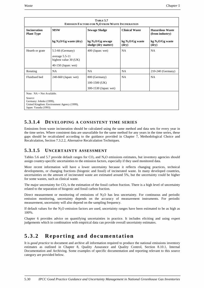
Waste Chapter 5
5.30 IPCC Good Practice Guidance and Uncertainty Management in National Greenhouse Gas Inventories
TABLE 5.7EMISSION FACTORS FOR N2O FROM WASTE INCINERATION
Incineration Plant Type
MSW Sewage Sludge Clinical Waste Hazardous Waste(from industry)
kg N2O/Gg waste (dry) kg N2O/Gg sewagesludge (dry matter)
kg N2O/Gg waste(dry)
kg N2O/Gg waste(dry)
Hearth or grate 5.5-66 (Germany)
average 5.5-11highest value 30 (UK)
40-150 (Japan: wet)
400 (Japan: wet) NA NA
Rotating NA NA NA 210-240 (Germany)
Fluidised bed 240-660 (Japan: wet) 800 (Germany)
100-1500 (UK)
300-1530 (Japan: wet)
NA NA
Note: NA = Not Available.
Source: Germany: Johnke (1999), United Kingdom: Environment Agency (1999), Japan: Yasuda (1993).
5.3.1.4 DEVELOPING A CONSISTENT TIME SERIESEmissions from waste incineration should be calculated using the same method and data sets for every year inthe time series. Where consistent data are unavailable for the same method for any years in the time series, thesegaps should be recalculated according to the guidance provided in Chapter 7, Methodological Choice andRecalculation, Section 7.3.2.2, Alternative Recalculation Techniques.
5.3.1.5 UNCERTAINTY ASSESSMENTTables 5.6 and 5.7 provide default ranges for CO2 and N2O emissions estimates, but inventory agencies shouldassign country-specific uncertainties to the emission factors, especially if they used monitored data.
More recent information will have a lower uncertainty because it reflects changing practices, technicaldevelopments, or changing fractions (biogenic and fossil) of incinerated waste. In many developed countries,uncertainties on the amount of incinerated waste are estimated around 5%, but the uncertainty could be higherfor some wastes, such as clinical waste.
The major uncertainty for CO2 is the estimation of the fossil carbon fraction. There is a high level of uncertaintyrelated to the separation of biogenic and fossil carbon fraction.
Direct measurement or monitoring of emissions of N2O has less uncertainty. For continuous and periodicemission monitoring, uncertainty depends on the accuracy of measurement instruments. For periodicmeasurement, uncertainty will also depend on the sampling frequency.
If default values for the N2O emission factors are used, uncertainty ranges have been estimated to be as high as100%.
Chapter 6 provides advice on quantifying uncertainties in practice. It includes eliciting and using expertjudgements which in combination with empirical data can provide overall uncertainty estimates.
5 . 3 . 2 R e p o r t in g a n d do c u me n t a t i o nIt is good practice to document and archive all information required to produce the national emissions inventoryestimates as outlined in Chapter 8, Quality Assurance and Quality Control, Section 8.10.1, InternalDocumentation and Archiving. Some examples of specific documentation and reporting relevant to this sourcecategory are provided below.

Chapter 5 Waste
IPCC Good Practice Guidance and Uncertainty Management in National Greenhouse Gas Inventories 5.31
It is not practical to include all documentation in the national inventory report. However, the inventory shouldinclude summaries of methods used and references to source data such that the reported emissions estimates aretransparent and steps in their calculation may be retraced.
Some countries use different categorisation schemes for waste at the local or regional level. In this case, theinventory agency should review consistency with the IPCC categorisation scheme and provide a rationale onhow it transformed the data to fit in the IPCC categories. Inventory agencies should clearly indicate the wastetypes included in the waste estimates.
Inventory agencies should also include information on how they obtained the carbon content, the fossil carbonfraction, and the N2O emission factors.
Many incineration plants produce electricity and heat. Combustion of waste for energy purposes should bereported under the Energy Sector of the IPCC Guidelines (CO2 from stationary combustion). Waste should bereported as ‘other fuel’ in the Energy Sector. These emissions should not be reported in the Waste Sector of theIPCC Guidelines so as to avoid double counting.
Sometimes gas, oil, or other fuels are used as support fuel to start the incineration process or maintain thetemperature. Consumption of support fuel for this purpose should not be reported under waste incineration butinstead included in the Energy Sector. Support fuels normally account for less than 3% of total calorific input,but they can be more important with the incineration of hazardous waste.
5 . 3 . 3 I n v en t o ry q u a l i t y a s su ra n c e / q u a l i ty c o n tr o l( Q A / Q C )
It is good practice to conduct quality control checks as outlined in Chapter 8, Quality Assurance and QualityControl, Table 8.1, Tier 1 General Inventory Level QC Procedures, and an expert review of the emissionsestimates. Additional quality control checks as outlined in the Tier 2 procedures in Chapter 8 and qualityassurance procedures may also be applicable, particularly if higher tier methods are used to determine emissionsfrom this source category. Inventory agencies are encouraged to use higher tier QA/QC for key source categoriesas identified in Chapter 7, Methodological Choice and Recalculation.
Furthermore, transparency can be improved by the provision of clear documentation and explanations of workundertaken in the following areas:
Review of direct emission measurements
• Where direct measurement data are available, inventory agencies should confirm that internationallyrecognised standard methods were used for measurements. If the measurement practices fail this criterion,then the use of these emissions data should be carefully evaluated.
• Where emissions are measured directly, inventory agencies should compare plant-level factors amongplants, and also to IPCC defaults. They should review any significant difference between factors.
Review of emission factors
• Inventory agencies should compare country-specific or plant-specific values of the carbon content of waste,the fossil carbon as fraction of total carbon, and the efficiency of combustion for the incinerator to thedefault values in Table 5.6.
• Inventory agencies should review the QC procedures associated with the waste incineration data andanalysis used to develop site-specific emission factors. If there is insufficient QC, the uncertainty of thenational estimates should be assessed and the use of those data may need to be evaluated.
Involvement of experts in the peer rev iew
• Expert peer review should be directed at the characterisations of waste fuel and situations where default dataare not used. This is particularly true for hazardous and clinical waste, because these wastes are often notquantified on a plant basis and can vary significantly from plant to plant.

Waste Chapter 5
5.32 IPCC Good Practice Guidance and Uncertainty Management in National Greenhouse Gas Inventories
R E F E R E N CE S
METHANE EMISSIONS FROM SOLID WASTE DISPOSAL SITESBingemer, H.G. and P.J. Crutzen (1987). ‘The production of methane from solid wastes.’ Journal of Geophysical
Research, 92 (D2), pp. 2181-2187.
Intergovernmental Panel on Climate Change (IPCC) (1997). Revised 1996 IPCC Guidelines for NationalGreenhouse Gas Inventories: Volume 3 Reference Manual. J.T. Houghton et al., IPCC/OECD/IEA, Paris,France.
Oonk, H. and T. Boom (1995). Landfill gas formation, recovery and emissions, TNO-report R95-203, TNO,Apeldoorn, The Netherlands.
EMISSIONS FROM WASTEWATER HANDLINGDoorn, M.R.J., R. Strait, W. Barnard, and B. Eklund (1997). Estimate of Global Greenhouse Gas Emissions from
Industrial and Domestic Wastewater Treatment, Final Report, EPA-600/R-97-091, Prepared for UnitedStates Environmental Protection Agency, Research Triangle Park, NC, USA.
Doorn, M.R.J. and D. Liles (1999). Global Methane, Quantification of Methane Emissions and Discussion ofNitrous Oxide, and Ammonia Emissions from Septic Tanks, Latrines, and Stagnant Open Sewers in theWorld. EPA-600/R-99-089, Prepared for U.S. EPA, Research Triangle Park, NC, USA.
Intergovernmental Panel on Climate Change (IPCC) (1997). Revised 1996 IPCC Guidelines for NationalGreenhouse Gas Inventories: Volume 3 Reference Manual. J.T. Houghton et al., IPCC/OECD/IEA, Paris,France.
Lexmond, M.J. and G. Zeeman (1995). Potential of controlled anaerobic wastewater treatment in order toreduce the global emissions of the greenhouse gases methane and carbon dioxide. Report No. 95-1,Department of Environmental Technology, Agricultural University of Wageningen, P.O. Box 8129, 6700 EVWageningen, The Netherlands.
EMISSIONS FROM WASTE INCINERATIONEnvironment Agency of the United Kingdom (1999). Environment Agency's Technical Guidance Notes,
Environment Agency’s Pollution Inventory (1998 Data), UK.
Intergovernmental Panel on Climate Change (IPCC) (1997). Revised 1996 IPCC Guidelines for NationalGreenhouse Gas Inventories: Volume 3 Reference Manual. J.T. Houghton et al., IPCC/OECD/IEA, Paris,France.
Johnke, B. (1999). ‘Emissions from waste incineration’. Background paper for Expert meeting on good practicein inventory preparation : emissions from waste. IPCC/OECD/IEA National Greenhouse Gas InventoriesProgramme, (Unpublished – TSU, Japan)
Yasuda, K. (1993). Emissions of Greenhouse Gases from Waste Incineration. Report of KanagawaEnvironmental Research Center, vol. 16, pp. 49-53, Kanagawa Environmental Research Center, Kanagawa,Japan.

Chapter 6 Quantifying Uncertainties in Practice
IPCC Good Practice Guidance and Uncertainty Management in National Greenhouse Gas Inventories 6.1
6
QUANTIFYING UNCERTAINTIES INPRACTICE

Quantifying Uncertainties in Practice Chapter 6
IPCC Good Practice Guidance and Uncertainty Management in National Greenhouse Gas Inventories6.2
CO-CHAIRS, EDITORS AND EXPERTS
Co-chairs of the Expert Meeting on Cross-sectoral Methodologies forUncertainty Estimation and Inventory QualityTaka Hiraishi (Japan) and Buruhani Nyenzi (Tanzania)
REVIEW EDITOR
Richard Odingo (Kenya)
Expert Group on Quantifying Uncertainties in PracticeCO-CHAIRS
Jim Penman (UK) and Semere Habetsion (Eritrea)
AUTHORS OF BACKGROUND PAPERS
Kay Abel (Australia), Simon Eggleston (UK) and Tinus Pullus (Netherlands)
CONTRIBUTORS
Simon Eggleston (UK), Christopher Frey (USA), Kari Gronfors (Finland), Niklas Höhne (UNFCCC Secretariat),Charles Jubb (Australia), Katarina Mareckova (Slovak Republic), Jeroen Meijer (IPCC-NGGIP/TSU), FrankNeitzert (Canada), Todd Ngara (Zimbabwe), Tinus Pulles (Netherlands), Emmanuel Rivière (France), ArthurRypinski (USA), Martiros Tsarukyan (Armenia), and Peter Zhou (Botswana)

Chapter 6 Quantifying Uncertainties in Practice
IPCC Good Practice Guidance and Uncertainty Management in National Greenhouse Gas Inventories 6.3
C o n t e n t s
6 QUANTIFYING UNCERTAINTIES IN PRACTICE
6.1 OVERVIEW..........................................................................................................................................6.5
6.2 IDENTIFYING UNCERTAINTIES .....................................................................................................6.6
6.2.1 Uncertainties associated with continuous monitoring of emissions ...........................................6.6
6.2.2 Uncertainties associated with direct determination of emission factors.....................................6.7
6.2.3 Uncertainties associated with emission factors from published references................................6.7
6.2.4 Uncertainties associated with activity data ................................................................................6.8
6.2.5 Expert Judgement ......................................................................................................................6.9
6.3 METHODS FOR COMBINING UNCERTAINTIES.........................................................................6.12
6.3.1 Comparison between tiers and choice of method.....................................................................6.13
6.3.2 Tier 1 – Estimating uncertainties by source category with simplifying assumptions ...............6.13
6.3.3 Tier 1 aggregation and reporting .............................................................................................6.18
6.4 TIER 2 – ESTIMATING UNCERTAINTIES BY SOURCE CATEGORYUSING MONTE CARLO ANALYSIS...............................................................................................6.18
6.4.1 Tier 2 uncertainties in trends ...................................................................................................6.21
6.4.2 Reporting Tier 2 uncertainty analysis ......................................................................................6.22
6.5 PRACTICAL CONSIDERATIONS IN USING MONTE CARLO SIMULATION ..........................6.24
6.5.1 Specifying probability distributions for inventory inputs.........................................................6.24
6.5.2 How much effort is needed to characterise uncertainty in an inventory input?........................6.25
6.5.3 Choosing a simulation technique and a simulation sample size...............................................6.26
6.5.4 Dependence and correlation among inventory inputs ..............................................................6.26
6.5.5 Does correlation matter?..........................................................................................................6.26
6.5.6 Some methods for dealing with dependencies or correlation...................................................6.27
6.5.7 Specifying correlation in inventory inputs ...............................................................................6.27
6.5.8 Analysing inventory outputs ....................................................................................................6.27
6.5.9 Encouragement of use of appropriate techniques ....................................................................6.27
6.6 CONCLUSION ...................................................................................................................................6.27
APPENDIX 6A.1 DERIVATION OF THE FORMULAE IN TABLE 6.1 (TIER 1)...............................6.28
APPENDIX 6A.2 TIER 1 UNCERTAINTY CALCULATION EXAMPLE ...........................................6.31
REFERENCES ............................................................................................................................................6.34

Quantifying Uncertainties in Practice Chapter 6
IPCC Good Practice Guidance and Uncertainty Management in National Greenhouse Gas Inventories6.4
F i g u r e s
Figure 6.1 Illustration of Monte Carlo Method ...............................................................................6.20
Figure 6.2 Example Frequency Plots of the Results of a Monte Carlo Simulation .........................6.21
Figure 6.3 Calculation Scheme for Monte Carlo Analysis of the Absolute Emissionsand the Trend of a Single Source Category, Estimated as Emission FactorTimes an Activity Rate ..................................................................................................6.22
T a b l e s
Table 6.1 Tier 1 Uncertainty Calculation and Reporting ...............................................................6.16
Table 6.2 Tier 2 Uncertainty Reporting .........................................................................................6.23
Table 6.3 Tier 1 Uncertainty Calculation and Reporting Example ................................................6.31

Chapter 6 Quantifying Uncertainties in Practice
IPCC Good Practice Guidance and Uncertainty Management in National Greenhouse Gas Inventories 6.5
6 QUANTIFYING UNCERTAINTIES INPRACTICE
6 . 1 O V E R V I E WThis chapter describes good practice in estimating and reporting uncertainties associated with both annualestimates of emissions, and emission trends over time. It identifies types of uncertainty from the viewpoint of theinventory practitioner and shows how to obtain expert judgements in a consistent manner. It provides two tiersfor combining source category uncertainties into an uncertainty estimate for total national emissions, and presentsan example of the application of the Tier 1 method.
The chapter is consistent with source-specific good practice guidance described in Chapters 2 to 5, the generalprinciples discussed in Annex 1, Conceptual Basis for Uncertainty Analysis, and the chapters on methodologicalchoice (Chapter 7, Methodological Choice and Recalculation) and QA/QC (Chapter 8, Quality Assurance andQuality Control).
Uncertainty estimates are an essential element of a complete emissions inventory. Uncertainty information is notintended to dispute the validity of the inventory estimates, but to help prioritise efforts to improve the accuracy ofinventories in the future and guide decisions on methodological choice, as indicated in Chapter 7,Methodological Choice and Recalculation. Inventory practitioners understand that for most countries and sourcecategories, greenhouse gas emissions estimates are reasonably accurate. However, national inventories preparedpursuant to the Revised 1996 IPCC Guidelines for National Greenhouse Gas Inventories (IPCC Guidelines) willtypically contain a wide range of emission estimates, varying from carefully measured and demonstrablycomplete data on emissions of certain engineered chemicals, to order-of-magnitude estimates of highly variablenitrous oxide (N2O) fluxes from soils and waterways.
Inventory estimates can be used for a range of purposes. For some purposes, only the national total matters, whilefor others, the detail by greenhouse gas and source category is important. In order to match the data to theintended purpose, users must be able to understand the actual reliability of both the total estimate and itscomponent parts. For this reason, the methods used to communicate uncertainty must be practical, scientificallydefensible, robust enough to be applicable to a range of source categories, methods and national circumstances,and presented in ways comprehensible to non-specialist inventory users.
There are many reasons that actual emissions and sinks may differ from the number calculated in a nationalinventory. These reasons are discussed at greater length in Annex 1. Some sources of uncertainty (i.e. samplingerror or limitations on instrument accuracy) may generate well-defined, easily characterised estimates of therange of potential error. However, other sources of uncertainty may be much more difficult to characterise. Thischapter describes how to account for both well-defined statistical uncertainties and less specific informationcharacterising other forms of uncertainty, and how to combine this information into a characterisation of theuncertainty of both the total inventory and its components.
Ideally, emissions estimates and uncertainty ranges would both be derived from source-specific measured data.Since it is not practical to measure every emission source in this way, estimates are often based on the knowncharacteristics of typical sources taken to be representative of the population. This introduces additionaluncertainties, because it must be assumed that the population of these sources behave, on average, like thesources that have been measured. Sometimes enough will be known about these typical sources to determine theiruncertainty distributions empirically. In practice, however, expert judgement will often be necessary to define theuncertainty ranges.
The pragmatic approach to producing quantitative uncertainty estimates in this situation is to use the bestavailable estimates; a combination of the available measured data and expert judgement. The methods proposedin this chapter can therefore be used with the source category-specific uncertainty ranges discussed in Chapters 2to 5, and also allow for new empirical data to be incorporated as they become available. This chapter alsodescribes methods for eliciting expert judgement in a way that minimises the risk of bias, and it discusses how tocombine uncertainties in emission factors and activity data to estimate source category and total uncertainties ininventories, as well as uncertainties in the trend.
The chapter uses two main statistical concepts – the probability density function and confidence limits – that aredefined formally in Annex 3, the Glossary, and discussed in more detail in Annex 1, Conceptual Basis for

Quantifying Uncertainties in Practice Chapter 6
IPCC Good Practice Guidance and Uncertainty Management in National Greenhouse Gas Inventories6.6
Uncertainty Analysis. Briefly, the probability density function describes the range and relative likelihood ofpossible values. Confidence limits give the range within which the underlying value of an uncertain quantity isthought to lie for a specified probability. This range is called the confidence interval. The IPCC Guidelinessuggest the use of a 95% confidence interval which is the interval that has a 95% probability of containing theunknown true value.
The analysis of uncertainty presented in this chapter does not consider the uncertainties in Global WarmingPotentials (GWPs). For reporting, the GWP values adopted at the Third Session of the UNFCCC Conference ofthe Parties become in effect fixed weighting factors. However, it should be kept in mind that GWP valuesactually have significant uncertainties associated with them and that an overall assessment of total equivalentemissions should take this fact into account.
6 . 2 I D E N T I F Y I N G U N C E R T A I N T I E SThe estimated uncertainty of emissions from individual sources (e.g. power plants, motor vehicles, dairy cattle) iseither a function of instrument characteristics, calibration and sampling frequency of direct measurements, or(more often) a combination of the uncertainties in the emission factors for typical sources and the correspondingactivity data. The uncertainties in the emission factors and activity data should be described using probabilitydensity functions. Where data are available to do so, the shape of the probability density function should bedetermined empirically. Otherwise, expert judgement will be necessary, following the rules set out in Section6.2.5, Expert Judgement, below. Sections 6.2.1 to 6.2.4 (below) give examples of typical situations that can ariseunder different circumstances of data availability. These subsections are ranked in order of their desirability inproducing uncertainty assessments.
Uncertainties are affected by choice of estimation algorithm, and this is reflected in good practice, where highertier methods (provided they are well implemented) should usually be associated with lower uncertainties. Ingeneral, uncertainties related to model choice will be reflected in the uncertainty ranges derived for use in thecontext of the model selected.
6 . 2 . 1 U n c e r t a i n t i e s a s s o c i a t e d w i t h c o n t i n u o u smo n i t o r i n g o f e mi s s i o n s
Continuous monitoring of emissions, though comparatively rare, is usually consistent with source category-specific good practice. In this case, the probability density function, and therefore the uncertainty in emissionsincluding 95% confidence limits, can be determined directly. Representative sampling requires that theequipment used to make the measurements be installed and operated according to the principles and referencesset out in Chapter 8 on QA/QC issues. Provided this is done, it is unlikely that there will be correlation of errorsbetween years. Therefore, the probability density function of the difference in emissions between two years (thetrend uncertainty) will be simply related to the probability density functions of the annual emissions. Assumingboth probability density functions are normal, the probability density function of the difference in emissions willalso be normal with:
EQUATION 6.1mean = µ1 – µ2
EQUATION 6.2standard deviation = (σ1
2 + σ22)1/2
where µ1 and µ2 are the mean values of the emissions in years t1 and t2, and σ1 and σ2 are the standard deviationsof the probability density functions of the emissions in year t1 and t2. The 95% confidence limits (this time of themean or the difference in the means) will be given by plus or minus approximately two standard deviations.1
1 For sample sizes less than about 30, a Student t distribution should be used to estimate confidence intervals.

Chapter 6 Quantifying Uncertainties in Practice
IPCC Good Practice Guidance and Uncertainty Management in National Greenhouse Gas Inventories 6.7
6 . 2 . 2 U n c e r t a i n t i e s a s s o c i a t e d w i t h d i r e c td e t e r mi n a t i o n o f e mi s s i o n f a c t o r s
In some cases, periodic emission measurements may be available at a site. If these measurements can be linked torepresentative activity data, which of course is crucial, then it is possible to determine a site-specific emissionfactor, together with an associated probability density function to represent annual emissions.
This can be a complex task. To achieve representativeness it may be necessary to partition (or stratify) the data toreflect typical operating conditions. For example:
• Start-up and shut down can give different emission rates relative to activity data. In this case, the datashould be partitioned, with separate emission factors and probability density functions derived for steadystate, start-up and shut down conditions.
• Emission factors can depend on load. In this case, the total emissions estimation and uncertainty analysismay need to be stratified to take account of load, expressed, for example, as percentage of full capacity. Thiscould be done by regression analysis and scatter plots of the emission rate against likely controlling variables(e.g. emissions versus load) with load becoming part of the activity data needed.
• Measurements taken for another purpose may not be representative. For example, methane measurementsmade for safety reasons at coal mines and landfills may not reflect total emissions. In such cases, the ratiobetween the measured data and total emissions should be estimated for the uncertainty analysis.
If the data sample size is large enough, standard statistical goodness-of-fit tests can be used, in combination withexpert judgement, to help in deciding which probability density function to use for describing variability in thedata (partitioned if necessary) and how to parameterise it. However, in many cases, the number of measurementsfrom which to make an inference regarding uncertainty will be small. Typically, as long as there are three or moredata points, and as long as the data are a random representative sample of the quantity of interest, it is possible toapply statistical techniques to estimate the values of the parameters of many two-parameter distributions (e.g.normal, lognormal) that can be used to describe variability in the data set (Cullen and Frey, 1999, pp. 116-117).With small sample sizes, there will be large uncertainties regarding the parameter estimates that should bereflected in the quantification of uncertainty for use in the emissions inventory. Furthermore, it is typically notpossible to rely on statistical methods to differentiate goodness-of-fit of alternative parametric distributions whensample sizes are very small (Cullen and Frey, 1999, pp. 158-159). Therefore, considerable judgement is requiredin selecting an appropriate parametric distribution to fit to a very small data set. In situations where thecoefficient of variation is less than approximately 0.3, a normal distribution may be a reasonable assumption(Robinson, 1989). When the coefficient of variation is large and the quantity is non-negative, then a positivelyskewed distribution such as a lognormal one may be appropriate. Guidance on the selection of distributions isprovided in Annex 1, Conceptual Basis for Uncertainty Analysis, and the use of expert judgements in this contextis outlined in Section 6.2.5, Expert Judgement, below.
6 . 2 . 3 U n c e r t a i n t i e s a s s o c i a t e d w i t h e mi s s i o nf a c t o r s f r o m p u b l i s h e d r e f e r e n c e s
When site-specific data are unavailable, good practice will usually be to develop emission estimates usingemission factors drawn from references consistent with the IPCC Guidelines and the source category-specificgood practice guidance described in Chapters 2 to 5. These factors will have been measured under particularcircumstances that are judged to be typical. There will be uncertainties associated with the originalmeasurements, as well as with the use of the factors in circumstances other than those associated with the originalmeasurements. It is a key function of good practice guidance for each source category to guide the choice ofemission factors to minimise this second source of uncertainty to the extent possible. The source category-specific guidance also indicates, wherever possible, the uncertainty ranges likely to be associated with using thesefactors.
Where such emission factors are used, the associated uncertainties should be estimated from:
• Original research including country-specific data. For measurement-based emission factors, the data fromthe original measurement programme may enable an assessment of the uncertainty and possibly theprobability density function. Well-designed measurement programmes will provide sample data that coverthe range of types of plants and their maintenance, size and age, so that the factors and their uncertainties can

Quantifying Uncertainties in Practice Chapter 6
IPCC Good Practice Guidance and Uncertainty Management in National Greenhouse Gas Inventories6.8
be used directly. In other cases, expert judgement will be needed to extrapolate from the measurements to thefull population of plants in that particular source/sink category.
• Good practice guidance. For most emission factors, source category-specific good practice guidanceprovides default uncertainty estimates that should be used in the absence of other information. Unless clearevidence to the contrary is available, the probability density functions are assumed to be normal. However,the inventory agency should evaluate the representativeness of the default for its own situation. If the defaultis judged to be unrepresentative and the source category is important to the inventory, improved assumptionsbased upon expert judgement should be developed.
An emission factor that over or underestimates emissions in the base year will probably do so in subsequentyears. Therefore, uncertainties due to emission factors will tend to be correlated over time.
6 . 2 . 4 U n c e r t a i n t i e s a s s o c i a t e d w i t h a c t i v i t y d a t aActivity data are often more closely linked to economic activity than are emission factors. There are often wellestablished price incentives and fiscal requirements for accurate accounting of economic activity. Activity datatherefore tend to have lower uncertainties and a lower correlation between years. Activity data are often collectedand published regularly by national statistical agencies. It is possible that these agencies have already assessedthe uncertainties associated with their data as part of their data collection procedures. These uncertainties can beused to construct probability density functions. This information will not necessarily have been published, so it isgood practice to contact the statistical agencies directly. Since economic activity data are not usually collectedfor the purpose of estimating greenhouse gas emissions, the applicability of the data should be assessed beforeusing them.
Examples of generic and specific questions that may arise on coverage, representativeness and repeatability fromyear to year are:
• Interpretation of statistical differences. Statistical differences in energy balance usually represent adifference between amount of reported primary fuels and amount of fuels identified in the categories ‘finalconsumption’ and ‘in transformation’. They can give an indication of the size of the uncertainties of the data,especially where long time series are considered.
• Interpretation of energy balances. Production, use and import/export data should be consistent. If not, thismay give an indication of the uncertainties.
• Cross-checks. It may be possible to compare two types of activity data that apply to the same source toprovide an indication of uncertainty ranges. For example, the sum of vehicle fuel use should becommensurate with the sum by vehicle type of the product of vehicle-km times fuel consumption efficiency.
• Vehicle numbers and types. Some countries maintain detailed vehicle registration databases with data onvehicles by type, age, fuel type and emission control technology, all of which can be important for a detailedbottom-up inventory of methane (CH4) and nitrous oxide (N2O) emissions from such vehicles. Others do nothave such detailed information and this will tend to increase the uncertainty.
• Smuggling of fuel across borders. This can be significant and may introduce bias into the activity data.Apparent consumption and the sum of the sectoral fuel use may be compared as a cross-check.
• Biomass fuels. Where formal markets for these fuels do not exist, consumption estimates may be much lessaccurate than for fuels in general.
• Livestock population data. Accuracy will depend on the extent and reliability of national census and surveymethods and there may be different accounting conventions for animals that do not live for a whole year.
Inventory agencies may also undertake dedicated research to collect additional activity data, consistent with goodpractice in the prioritisation of efforts toward key source categories (i.e. those source categories with asignificant influence on a country’s total inventory of direct greenhouse gases in terms of the absolute level ofemissions, the trend in emissions, or both, as described in Chapter 7, Methodological Choice and Recalculation).
Probability density functions associated with activity data can be difficult to assess. The procedures outlined inthis chapter should be applied to the available information, in accordance with the advice on interpreting expertjudgements in the following section.

Chapter 6 Quantifying Uncertainties in Practice
IPCC Good Practice Guidance and Uncertainty Management in National Greenhouse Gas Inventories 6.9
6 . 2 . 5 E x p e r t j u d g e me n tEstimates of uncertainty in emission factors or direct emission measurements will need to be based on expertjudgement when empirical data are lacking. Estimates of uncertainty in activity data will often be based on expertjudgement, informed wherever possible by cross-checks like those described in the previous section.
Experts are people who have special skills or knowledge in a particular field. A judgement is the forming of anestimate or conclusion from information presented to or available to the expert. It is important to selectappropriate experts with respect to the emission inventory inputs for which uncertainty estimates are needed.
The goal of expert judgement here is to develop a probability density function, taking into account relevantinformation such as:
• Is the emission source similar to other sources? How is the uncertainty likely to compare?
• How well is the emission process understood? Have all possible emission sources been identified?
• Are there physical limits on how much the emission factor can vary? Unless the process is reversible itcannot emit less than zero, and this may constrain a very wide uncertainty range. Mass balanceconsiderations or other process data may place an upper limit on emissions.
• Are the emissions consistent with atmospheric concentrations? Emissions are reflected in atmosphericconcentrations at site-specific and larger scales and again this may limit the possible emission rates.
A degree of expert judgement is required even when applying classical statistical techniques to data sets, sinceone must judge whether the data are a representative random sample and, if so, what methods to use to analysethe data. This may require both technical and statistical judgement. Interpretation is especially needed for datasets that are small, highly skewed or censored.2 The formal methods for obtaining data from experts are known asexpert elicitation.
POSSIBLE BIASES IN EXPERT ELICITATIONWherever possible, expert judgement regarding uncertainty should be elicited using an appropriate protocol.Once experts are identified, elicitation protocols should be designed to overcome the biases that can beintroduced by the rules of thumb (sometimes called heuristics) that experts use when formulating judgementsabout uncertainty.
The most common unconscious biases introduced by rules of thumb are:
• Availability bias. This is basing judgements on outcomes that are more easily remembered.
• Representativeness bias. This is basing judgements on limited data and experience without fully consideringother relevant evidence.
• Anchoring and adjustment bias. This is fixating on a particular value in a range and making insufficientadjustments away from it in constructing an uncertainty estimate.
To counteract the first two potential sources of biases, elicitation protocols should include a review of relevantevidence. In order to counteract the third potential source of bias, it is important to ask the expert to makejudgements regarding extreme values first, before asking for judgements regarding central values of adistribution. When an expert gives too narrow a range of values, that is said to be ‘overconfidence’. Experts oftensystematically underestimate uncertainties according to Morgan and Henrion (1990). It is desirable to avoidoverconfidence so as not to underestimate the true uncertainty.
There is also the possibility of more conscious biases:
• Motivational bias is a desire by an expert to influence an outcome or to avoid contradicting prior positionson an issue.
• Expert bias arises from an unqualified expert’s desire to appear as a true expert in the field. This wouldtypically lead to overconfident estimates of uncertainty.
2 In these cases it may be helpful to consider a numerical method, such as the bootstrap, for characterising samplingdistributions. Methods for characterising sampling distributions for the mean are described by Cullen and Frey (1999), Freyand Rhodes (1996), and Frey and Burmaster (1999).

Quantifying Uncertainties in Practice Chapter 6
IPCC Good Practice Guidance and Uncertainty Management in National Greenhouse Gas Inventories6.10
• Managerial bias is a situation in which an expert makes judgements that achieve organisational goals, ratherthan judgements that reflect the actual state of knowledge regarding an inventory input.
• Selection bias occurs when the inventory agency selects the expert who tells it what it wants to hear.
The best way to avoid these biases is to be careful in the selection of experts.
Expert judgements can be elicited from individuals or groups. Groups can be useful for sharing knowledge andhence could be part of the motivation, structuring, and conditioning steps of the elicitation. However, groupdynamics may introduce other biases. Thus, it is usually preferable to elicit judgement on an individual basis.
A PROTOCOL FOR EXPERT ELICITATIONAn example of a well-known protocol for expert elicitation is the Stanford/SRI protocol. Its five steps aredescribed below, and an example of its use is presented in Box 6.1, A Brief Example of Detailed ExpertJudgement.
• Motivating: Establish a rapport with the expert, and describe the context of the elicitation. Explain theelicitation method to be used and the reason it was designed that way. The elicitor should also try to explainthe most commonly occurring biases to the expert, and to identify possible biases in the expert.
• Structuring: Clearly define the quantities for which judgements are to be sought, including, for example, theyear and country, the emission source category, the averaging time to be used (one year), the focus onuncertainty in the mean value of emission factors, and the structure of the emission inventory model. Clearlyidentify conditioning factors and assumptions (e.g. emissions should be for typical conditions averaged overa one-year period).
• Conditioning: Work with the expert to identify all relevant data, models, and theory pertaining to thequantity for which judgements about uncertainty are required.
• Encoding: Request the expert’s judgement regarding uncertainty. The next section on encoding describessome alternative methods to use.
• Verification: Analyse the expert’s response and provide the expert with feedback as to what has beenconcluded regarding his or her judgement. Is what has been encoded really what the expert meant? Are thereinconsistencies in the expert’s judgement?
METHODS FOR ENCODING EXPERT JUDGEMENTSThe method to be used in the encoding step should depend upon the expert’s familiarity with probabilitydistributions. Some commonly used methods are:
• Fixed Value: Estimate the probability of being higher (or lower) than an arbitrary value and repeat, typicallythree or five times. For example, what is the probability that an emission factor would be less than 100?
• Fixed Probability: Estimate the value associated with a specified probability of being higher (or lower). Forexample, what is the emission factor such that there is only a 2.5 percent probability (or 1 in 40 chance) thatthe emission factor could be lower (or higher) than that value.
• Interval Methods: This method focuses on the median and the quartiles. For example, the expert would beasked to choose a value of the emission factor such that it is equally likely that the true emission factorwould be higher or lower than that value. This yields the median. Then the expert would divide the lowerrange into two bins such that he or she felt it to be equally likely (25 percent probability) that the emissionfactor could be in either bin, and this would be repeated for the other end of the distribution. Finally, eitherfixed probability or fixed value methods could be used to get judgements for extreme values.
• Graphing: The expert draws his/her own distributions. This should be used cautiously because some expertsare overconfident about their knowledge of probability distributions.

Chapter 6 Quantifying Uncertainties in Practice
IPCC Good Practice Guidance and Uncertainty Management in National Greenhouse Gas Inventories 6.11
BOX 6.1
A BRIEF EXAMPLE OF DETAILED EXPERT JUDGEMENT
Suppose that the inventory agency has identified an expert regarding emissions of methane frompower plants, and wish to obtain her judgement regarding the uncertainty in annual averageemissions for this source category. As part of the motivation step, the elicitor has explained to theexpert the general purpose of the analysis and the expert elicitation protocol to be used. In thestructuring step, the elicitor works with the expert to set up the specific elicitation protocol. Forexample, although all the inventory agency may want is an annual average uncertainty estimate, theexpert may tell the elicitor that she prefers to provide judgements separately for start-up, part load,and full load operation of the plant, and that these three judgements should be weighted in order tocome up with the combined uncertainty for an annual average. After structuring the problem, theelicitor then reviews the expert information relevant to the assessment, such as measurements thatmay have been made on similar types of power plants or other combustion sources. In theelicitation step, the elicitor might ask the expert for an upper value such that there is only a one in40 chance (2.5 percent probability) of obtaining a higher value. After getting the value, the elicitorasks the expert to explain the logical basis for this estimate, such as the scenario of operation at theplant that might lead to such a high emission rate. Then the process might be repeated for the lowerend of the range, and perhaps for the median, 25th percentile, and 75th percentile. A mixture offixed value and fixed probability questions might be used. The elicitor should plot these on a graphso that any inconsistencies can be identified and corrected during the time available with theexpert. In the verification step, the elicitor would make sure that the expert is comfortable that theirjudgement has been well represented. The elicitor might also see how the expert would react to thepossibility of values outside of the interval for which judgements were provided, so as to ensurethat the expert is not being overconfident.
Sometimes the only available expert judgement will consist of a range, perhaps quoted together with a mostlikely value. Under these circumstances the following rules apply:
• Where experts only provide an upper and a lower limiting value, assume the probability density function isuniform and that the range corresponds to the 95% confidence interval.
• Where experts also provide a most likely value, assume a triangular probability density function using themost likely values as the mode and assuming that the upper and lower limiting values each exclude 2.5% ofthe population. The distribution need not be symmetrical.
Some other sources of information on expert elicitation include Spetzler and von Holstein (1975), Morgan andHenrion (1990), Merkhofer (1987), Hora and Iman (1989), and NCRP (1996).
The subjective nature of expert judgement increases the need for quality assurance and quality control proceduresto improve comparability of uncertainty estimates between countries. Therefore expert judgements should bedocumented as part of the national archiving process, and inventory agencies are encouraged to review expertjudgements, particularly for key source categories. Documentation should include:
• Reference number for judgement;
• Date;
• Person(s) involved and affiliation;
• The quantity being judged;
• The logical basis for judgement, including any data taken into consideration;
• The resultant probability distribution, or the range and most likely value and the probability distributionsubsequently inferred;
• Identification of any external reviewers;
• Results of any external review;
• Approval by inventory agency, specifying date and person.

Quantifying Uncertainties in Practice Chapter 6
IPCC Good Practice Guidance and Uncertainty Management in National Greenhouse Gas Inventories6.12
6 . 3 M E T H O D S F O R C O M B I N I N GU N C E R T A I N T I E S
Once the uncertainties in the source categories have been determined, they may be combined to provideuncertainty estimates for the entire inventory in any year and the uncertainty in the overall inventory trend overtime.
The error propagation equation, as discussed more extensively in Annex 1 of this report, and in Annex I of theIPCC Guidelines (Reporting Instructions), yields two convenient rules for combining uncorrelated uncertaintiesunder addition and multiplication:
• Rule A: Where uncertain quantities are to be combined by addition, the standard deviation of the sum will bethe square root of the sum of the squares of the standard deviations of the quantities that are added with thestandard deviations all expressed in absolute terms (this rule is exact for uncorrelated variables).
Using this interpretation, a simple equation can be derived for the uncertainty of the sum, that whenexpressed in percentage terms becomes:
EQUATION 6.3
n21
2nn
222
211
total x...xx)x (U...) x (U) x (U
U+++
•++•+•=
Where:
Utotal is the percentage uncertainty in the sum of the quantities (half the 95% confidence interval dividedby the total (i.e. mean) and expressed as a percentage);
xi and Ui are the uncertain quantities and the percentage uncertainties associated with them, respectively.
• Rule B: Where uncertain quantities are to be combined by multiplication, the same rule applies except thatthe standard deviations must all be expressed as fractions of the appropriate mean values (this rule isapproximate for all random variables).
A simple equation can also be derived for the uncertainty of the product, expressed in percentage terms:
EQUATION 6.42n
22
21total U...UUU +++=
Where:
Utotal is the percentage uncertainty in the product of the quantities (half the 95% confidence interval dividedby the total and expressed as a percentage);
Ui are the percentage uncertainties associated with each of the quantities.
The greenhouse gas inventory is principally the sum of products of emission factors and activity data. Therefore,Rules A and B can be used repeatedly to estimate the uncertainty of the total inventory. In practice, uncertaintiesfound in inventory source categories vary from a few percent to orders of magnitude, and may be correlated. Thisis not consistent with the assumptions of Rules A and B that the variables are uncorrelated with a standarddeviation of less than about 30% of the mean, but under these circumstances, Rules A and B may still be used toobtain an approximate result. Alternatively, a stochastic simulation (the Monte Carlo method) can be used, thatcan combine uncertainties with any probability distribution, range, and correlation structure, provided they havebeen suitably quantified. Thus, two tiers for uncertainty analysis are described below:
• Tier 1: Estimation of uncertainties by source category using the error propagation equation via Rules A andB, and simple combination of uncertainties by source category to estimate overall uncertainty for one yearand the uncertainty in the trend.
• Tier 2: Estimation of uncertainties by source category using Monte Carlo analysis, followed by the use ofMonte Carlo techniques to estimate overall uncertainty for one year and the uncertainty in the trend.

Chapter 6 Quantifying Uncertainties in Practice
IPCC Good Practice Guidance and Uncertainty Management in National Greenhouse Gas Inventories 6.13
Monte Carlo analysis can also be used in a restricted way within Tier 1 to combine activity data and emissionfactor uncertainties that have very wide or non-normal probability distributions or both. This approach can alsohelp deal with source categories within Tier 1 that are estimated by process models, rather than by the classical‘emission factor times activity data’ calculation. The choice between methods is discussed in Section 6.3.1below.
6 . 3 . 1 C o mp a r i s o n b e t w e e n t i e r s a n d c h o i c e o fme t h o d
Use of either Tier 1 or Tier 2 will provide far greater insight than previously available into how individual sourcecategories and greenhouse gases contribute to uncertainty in total emissions in any year, and to the trend in totalemissions between years.
Application of Tier 2 to the UK inventory (Eggleston et al., 1998) suggests that the 95% confidence interval isasymmetric and lies between about 7% below and 20% above the mean. Application of Tier 1 (see Appendix6A.2, Tier 1 Uncertainty Calculation Example) suggests an uncertainty of about ±20%. Since the approximationsinherent in Tier 1 mean that it cannot deal with asymmetry, this comparison is encouraging. Physically, thereason for the asymmetry identified under Tier 2 is that the uncertainty range of some very uncertain sourcecategories is constrained by the knowledge that the emissions cannot be less than zero. The Tier 2 method canmake use of this extra knowledge, but the Tier 1 method cannot. On trends between years, the Tier 2 study byEggleston et al. suggests that the 95% confidence interval is roughly symmetrical and lies between 5% above and5% below the mean.3 The corresponding Tier 1 result gives a range of about ±2%. The lower Tier 1 value ispartly because the trend estimated here is for the period 1990 to 1997, whereas the Tier 2 estimate was for 1990to 2010, but this is unlikely to account for all the differences. Nevertheless, both methods still give similarmagnitudes in the trend uncertainty that is less than the uncertainty in total emissions in any year.
Further national comparisons between methods would be very useful in developing understanding. The Tier 1method, being spreadsheet based, is very easy to apply and would represent hardly any additional effort for aninventory agency also undertaking Tier 2. Therefore, for the present, it is good practice for all countriesundertaking uncertainty analysis to report Tier 1 results, and for all inventory agencies with sufficient resourcesand expertise to undertake Tier 2.
6 . 3 . 2 T i e r 1 – E s t i ma t i n g u n c e r t a i n t i e s b y s o u r c ec a t e g o r y w i t h s i mp l i f y i n g a s s u mp t i o n s
The Tier 1 analysis estimates uncertainties by using the error propagation equation in two steps. First, the Rule Bapproximation is used to combine emission factor and activity data ranges by source category and greenhousegas. Second, the Rule A approximation is used to arrive at the overall uncertainty in national emissions and thetrend in national emissions between the base year and the current year.
The Tier 1 approach should be implemented using Table 6.1, Tier 1 Uncertainty Calculation and Reporting thatcan be set up on commercial spreadsheet software. The table is completed at the source category level usinguncertainty ranges for activity data and emission factors consistent with the sectoral good practice guidance inChapters 2 to 5. Different gases should be entered separately as CO2 equivalents (i.e. the emissions should bemultiplied by 100-year GWP values). Trend uncertainties are estimated using two sensitivities:
• Type A sensitivity: the change in the difference in overall emissions between the base year and the currentyear, expressed as a percentage, resulting from a 1% increase in emissions of a given source category andgas in both the base year and the current year.
• Type B sensitivity: the change in the difference in overall emissions between the base year and the currentyear, expressed as a percentage, resulting from a 1% increase in emissions of a given source category andgas in the current year only.
Conceptually, Type A sensitivity arises from uncertainties that affect emissions in the base year and the currentyear equally, and Type B sensitivity arises from uncertainties that affect emissions in the current year only.Uncertainties that are fully correlated between years will be associated with Type A sensitivities, and 3 Specifically a fall in emissions of 6 ±5%.

Quantifying Uncertainties in Practice Chapter 6
IPCC Good Practice Guidance and Uncertainty Management in National Greenhouse Gas Inventories6.14
uncertainties that are not correlated between years will be associated with Type B sensitivities. The discussion inSections 6.2.1 to 6.2.4 above suggests that emission factor uncertainties will tend to have Type A sensitivities,and activity data uncertainties will tend to have Type B. However, this association will not always hold and it ispossible to apply Type A sensitivities to activity data, and Type B sensitivities to emission factors to reflectparticular national circumstances. Type A and Type B sensitivities are simplifications introduced for the analysisof correlation.
Once the uncertainties introduced into national emissions by Type A and Type B sensitivities have beencalculated, they can be summed using the error propagation equation (Rule A) to give the overall uncertainty inthe trend.
The columns of Table 6.1, Tier 1 Uncertainty Calculation and Reporting, are labelled A to Q and contain thefollowing information:
• A and B show the IPCC source category and greenhouse gas.
• C and D are the inventory estimates in the base year and the current year4 respectively, for the sourcecategory and gas specified in columns A and B, expressed in CO2 equivalents.
• E and F contain the uncertainties for the activity data and emission factors respectively, derived from amixture of empirical data and expert judgement as previously described in this chapter, entered as half the95% confidence interval divided by the mean and expressed as a percentage. The reason for halving the 95%confidence interval is that the value entered in columns E and F then corresponds to the familiar plus orminus value when uncertainties are loosely quoted as ‘plus or minus x%’, so expert judgements of this typecan be directly entered in the spreadsheet. If uncertainty is known to be highly asymmetrical, enter the largerpercentage difference between the mean and the confidence limit.
• G is the combined uncertainty by source category derived from the data in columns E and F using the errorpropagation equation (Rule B). The entry in column G is therefore the square root of the sum of the squaresof the entries in columns E and F.
• H shows the uncertainty in column G as a percentage of total national emissions in the current year. This is ameasure of the degree of uncertainty introduced into the national emissions total by the source category inquestion. The entry in each row of column H is the entry in column G multiplied by the entry in column D,divided by the total at the foot of column D. The total at the foot of column H is an estimate of thepercentage uncertainty in total national emissions in the current year, calculated from the entries above usingRule A. This total is obtained by summing the squares of all the entries in column H and taking the squareroot.
• I shows how the percentage difference in emissions between the base year and the current year changes inresponse to a one percent increase in source category emissions in both the base year and the current year.This shows the sensitivity of the trend in emissions to a systematic uncertainty in the emissions estimate (i.e.one that is correlated between the base year and the current year). This is the Type A sensitivity as definedabove. Appendix 6A.1 provides the derivation for the formula for the entries in column I.
• J shows how the percentage difference in emissions between the base year and the current year changes inresponse to a one percent increase in source category emissions in the current year only. This shows thesensitivity of the trend in emissions to random error in the emissions estimate (i.e. one, that is not correlated,between the base year and the current year). This is the Type B sensitivity as described above. The formulafor the entries in column J is derived in Appendix 6A.
• K uses the information in columns I and F to show the uncertainty introduced into the trend in emissions byemission factor uncertainty, under the assumption that uncertainty in emission factors is correlated betweenyears. If the user decides that the emission factor uncertainties are not correlated between years then theentry in column J should be used in place of that in column I and the result multiplied by √2. The formula forthe entries in column K is derived in Appendix 6A.
• L uses the information in columns J and E to show the uncertainty introduced into the trend in emissions byactivity data uncertainty, under the assumption that uncertainty in activity data is not correlated betweenyears. If the user decides that the activity data uncertainties are correlated between years then the entry incolumn I should be used in place of that in column J and the √2 factor does not then apply. The formula forthe entries in column L is derived in Appendix 6A.
4 The current year is the most recent year for which inventory data are available.

Chapter 6 Quantifying Uncertainties in Practice
IPCC Good Practice Guidance and Uncertainty Management in National Greenhouse Gas Inventories 6.15
• M is an estimate of the uncertainty introduced into the trend in national emissions by the source category inquestion. Under Tier 1, this is derived from the data in columns K and L using Rule B. The entry in columnM is therefore the square root of the sum of the squares of the entries in columns K and L. The total at thefoot of this column is an estimate of the total uncertainty in the trend, calculated from the entries above usingthe error propagation equation. This total is obtained by summing the squares of all the entries in column Mand taking the square root. The formula for the entries in column M and the total at the foot of column M isshown in Appendix 6A.1.
• Columns N to Q are used for indicators and cross referencing to footnotes.
• N contains D, M or R, depending on whether the emission factor uncertainty range is based on default (D)information in source category guidance, measurements (M) made for the purpose or national referenced (R)information.
• O contains D, M or R, depending on whether the activity data uncertainty range is based on defaultinformation in sector guidance, measurements made for the purpose or national referenced information.
• P contains the reference numbers of any expert judgements used to estimate uncertainties in this sourcecategory.
• Q contains the number of an explanatory footnote to go at bottom of table to identify documentary referenceof uncertainty data (including measured data) or other comments relevant to the line.
An example of the spreadsheet with all the numerical data completed is provided in Appendix 6A.2, Tier 1uncertainty calculation example.
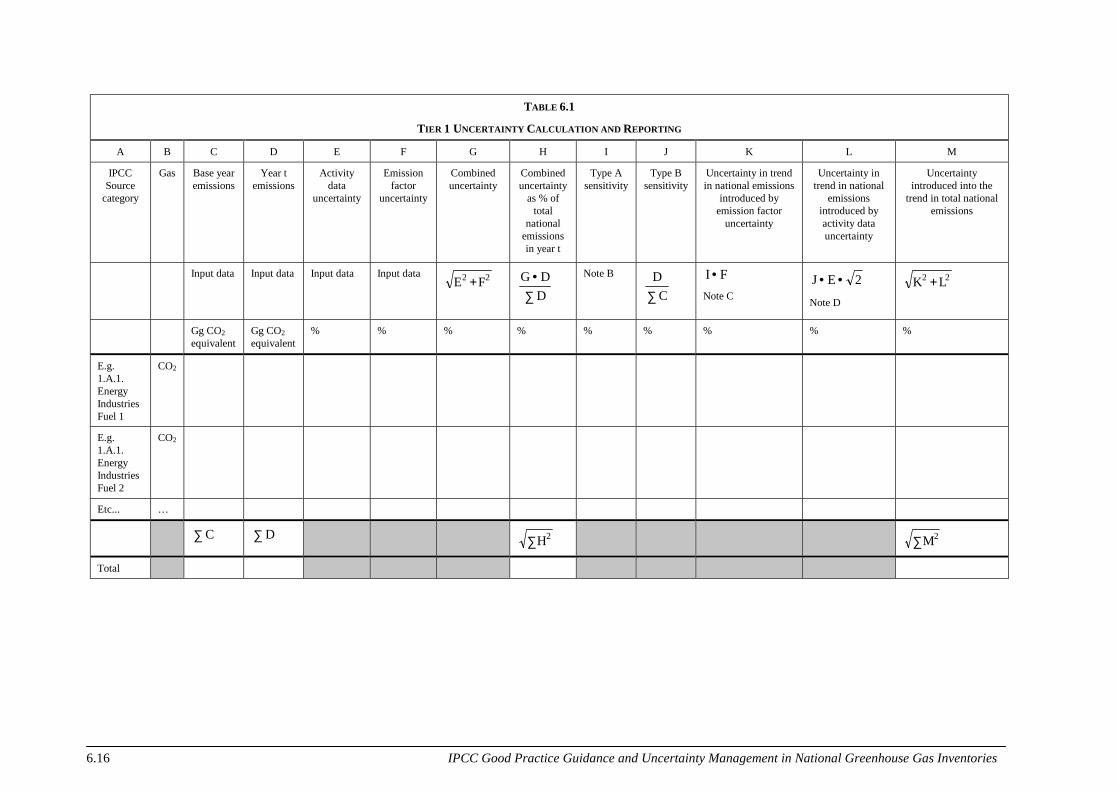
IPCC Good Practice Guidance and Uncertainty Management in National Greenhouse Gas Inventories6.16
TABLE 6.1
TIER 1 UNCERTAINTY CALCULATION AND REPORTING
A B C D E F G H I J K L M
IPCCSource
category
Gas Base yearemissions
Year temissions
Activitydata
uncertainty
Emissionfactor
uncertainty
Combineduncertainty
Combineduncertainty
as % oftotal
nationalemissionsin year t
Type Asensitivity
Type Bsensitivity
Uncertainty in trendin national emissions
introduced byemission factor
uncertainty
Uncertainty intrend in national
emissionsintroduced byactivity datauncertainty
Uncertaintyintroduced into the
trend in total nationalemissions
Input data Input data Input data Input data 22 FE +∑
•DDG Note B
∑ CD FI •
Note C2EJ ••
Note D
22 LK +
Gg CO2equivalent
Gg CO2equivalent
% % % % % % % % %
E.g.1.A.1.EnergyIndustriesFuel 1
CO2
E.g.1.A.1.EnergyIndustriesFuel 2
CO2
Etc... …
∑ C ∑ D ∑ 2H ∑ 2M
Total

IPCC Good Practice Guidance and Uncertainty Management in National Greenhouse Gas Inventories6.17
TABLE 6.1 (CONTINUED)
TIER 1 UNCERTAINTY CALCULATION AND REPORTING
A(continued)
B(continued)
N O P Q
IPCCSourcecategory
Gas Emissionfactor qualityindicator
Activity dataqualityindicator
Expertjudgementreferencenumbers
Footnotereferencenumber
Note E Note E
E.g.1.A.1.EnergyIndustries
Fuel 1
CO2
E.g.1.A.1.EnergyIndustriesFuel 2
CO2
Etc... …
Total
Note A If only total uncertainty is known for a source category (not for emission factor and activity data separately), then:
• If uncertainty is correlated across years, enter the uncertainty into column F, and enter 0 in column E;
• If uncertainty is not correlated across years, enter the uncertainty into column E and enter 0 in column F.

Quantifying uncertainties in Practice Chapter 6
IPCC Good Practice Guidance and Uncertainty Management in National Greenhouse Gas Inventories6.18
Note B
100C
CD100
)CC(0.01)CC(0.01DD0.01
i
ii
ix
ixix •∑
∑ ∑−−•
∑+•∑ ∑+•−+•
Note C
In the case where no correlation between emission factors is assumed, sensitivity B should be used and the resultmultiplied by √2:
2FJK xxx ••=
Note D
In the case where correlation between activity data is assumed, sensitivity A should be used and the √2 is notrequired:
xxx EIL •=
Note E
Please use the following abbreviations:D – IPCC source category defaultM – measurement basedR – national referenced data
6 . 3 . 3 T i e r 1 a g g r e g a t i o n a n d r e p o r t i n gTable 6.1, Tier 1 Uncertainty Calculation and Reporting, has one line for each source category, fuel (whereappropriate), and greenhouse gas and should be used for reporting.
Although the Tier 1 method allows for correlation over time, as described above, it does not account forcorrelation and dependency between source categories that may occur because the same activity data or emissionfactors may be used for multiple estimates. Often one gas dominates the source category and this reduces theeffect of any correlation. However, correlation and dependency may be significant for fossil fuels because a givenfuel is used with the same emission factor across several sub-categories, and if (as is sometimes the case) totalconsumption of a fuel is better known than consumption disaggregated by source category, hidden dependencieswill exist within the statistics because of the constraint provided by overall consumption. Dependency andcorrelation can be addressed by aggregating the source categories to the level of overall consumption ofindividual fuels before the uncertainties are combined. This entails some loss of detail in reporting onuncertainties but will deal with the dependencies where they are thought to be significant (e.g. where theuncertainties in fossil fuel emissions when aggregated from the source category level are greater than expected).The example Tier 1 calculation using UK data provided in Appendix 6A.2 has fossil fuel categories aggregatedin this way. This has the advantage of allowing compatibility with the categories suggested in Chapter 7 for thekey source category analysis.
6 . 4 T I E R 2 – E S T I M A T I N G U N C E R T A I N T I E S B YS O U R C E C A T E G O R Y U S I N G M O N T E C A R L OA N A L Y S I S
Under Tier 2, the simplifying assumptions required for Tier 1 can be relaxed. Tier 2 uses Monte Carlo analysis tocombine source category uncertainties.
The principle of Monte Carlo analysis is to select random values of emission factor and activity data from withintheir individual probability density functions, and to calculate the corresponding emission values. This procedureis repeated many times, using a computer, and the results of each calculation run build up the overall emissionprobability density function. Monte Carlo analysis can be performed at the source category level, foraggregations of source categories or for the inventory as a whole.
Monte Carlo analysis can deal with probability density functions of any physically possible shape and width, canhandle varying degrees of correlation (both in time and between source categories) and can deal with more

Chapter 6 Quantifying Uncertainties in Practice
IPCC Good Practice Guidance and Uncertainty Management in National Greenhouse Gas Inventories 6.19
complex models (e.g. the 1st order decay for CH4 from landfills) as well as simple ‘emission factor times activitydata’ calculations.
Eggleston et al. (1998) provide an example of Monte Carlo analysis, applied to a national greenhouse gasinventory and used to estimate uncertainties both in overall emissions and emissions trends. Another example ofthe use of Monte Carlo analysis is given in McCann et al. (1994). A general description of the Monte Carlomethod can be found in Fishman (1996).
Like all methods, Monte Carlo analysis only provides satisfactory results if it is properly implemented. Thisrequires the analyst to have scientific and technical understanding of the inventory. Of course, the results willonly be valid to the extent that the input data, including any expert judgements, are sound.
The Monte Carlo approach consists of five clearly defined steps shown in Figure 6.1. Only the first two of theserequire effort from the user, the remainder being handled by the software package. Section 6.5.3 contains a shortdiscussion of various software packages.
• Step 1 – Specify source category uncertainties. Specify the uncertainties in the basic data. This includesemission factors and activity data, their associated means and probability distribution functions, and anycross correlation between source categories. Take account of the information in Sections 6.2.1 to 6.2.5.
• Step 2 – Set up software package. The emission inventory calculation, the probability density functionsand the correlation values should be set up in the Monte Carlo package.
The software automatically performs the subsequent steps.
• Step 3 – Select random variables. This is the start of the iterations. For each input data item, emissionfactor or activity data, a number is randomly selected from the probability density function of that variable.
• Step 4 – Estimate emissions. The variables selected in Step 3 are used to estimate total emissions. Theexample given in Figure 6.1 assumes three source categories, each estimated as activity multiplied by anemission factor, and then summed to give total emissions. The calculations can be more complex. Emissionsby gas can be multiplied by GWP values, in order to obtain total national emissions in CO2 equivalent.Correlations of 100% are easy to incorporate, and good Monte Carlo packages allow other correlations to beincluded. Since the emission calculations should be the same as those used to estimate the national inventory,the Monte Carlo process could be fully integrated into the annual emission estimates.
• Step 5 – Iterate and monitor results. The calculated total from step 4 is stored, and the process thenrepeats from step 3. The mean of the totals stored gives an estimate of the total emission. Their distributiongives an estimate of the probability density function of the result. As the process repeats, the meanapproaches the final answer. When the mean no longer changes by more than a predefined amount, thecalculation can be terminated. When the estimate for the 95% confidence range is determined to within ±1%, then an adequately stable result has been found. Convergence can be checked by plotting a frequencyplot of the estimates of the emission. This plot should be reasonably smooth (Figure 6.2, Example frequencyplots of the results of a Monte Carlo simulation). These actions should be handled by the software, with theuser specifying either a number of iterations or convergence criteria.

Quantifying uncertainties in Practice Chapter 6
IPCC Good Practice Guidance and Uncertainty Management in National Greenhouse Gas Inventories6.20
F i g u r e 6 . 1 I l l u s t r a t i o n o f M o n t e C a r l o M e t h o d
Selectrandom valueof EmissionFactor fromdistribution
Selectrandom value
of ActivityData from
distribution
Pro
babi
lity
Va lue
Pro
babi
lity
Va luePro
babi
lity
Va luePro
babi
lity
Va luePro
babi
lity
Va lue Pro
babi
lity
Va lue
EstimateEmissions -
Mu ltiply Numbers
Selectrandom valueof EmissionFactor fromdistribution
Selectrandom value
of ActivityData from
distribution
Selectrandom valueof EmissionFactor fromdistribution
Selectrandom value
of ActivityData from
distribution
EstimateEmissions -
Mu ltiply Numbers
EstimateEmissions -
Mu ltiply Numbers
Add secto remissions to give
tota l
Store EmissionTotal in
database ofresults
Repeat until meanand distribution do
not change
Step 1 and 2 – Specify Uncertainties, W idth and Probability D istributionFunctions (pdfs) for all input data and set up softw are package
Step 3 - Select values fo r variables from the probability d istributions
Step 4 - C alculate E m issions in the conventional w ay
Repeat Step 2More iterations
Calcula te overallmean and
uncertainty fromdatabase of results
F in ished
Step 5 - Iterate and m onitor results
Source A Source CSource B
This example assumes three emission source categories each where the emission is calculated asActivity Data • Emission Factor.
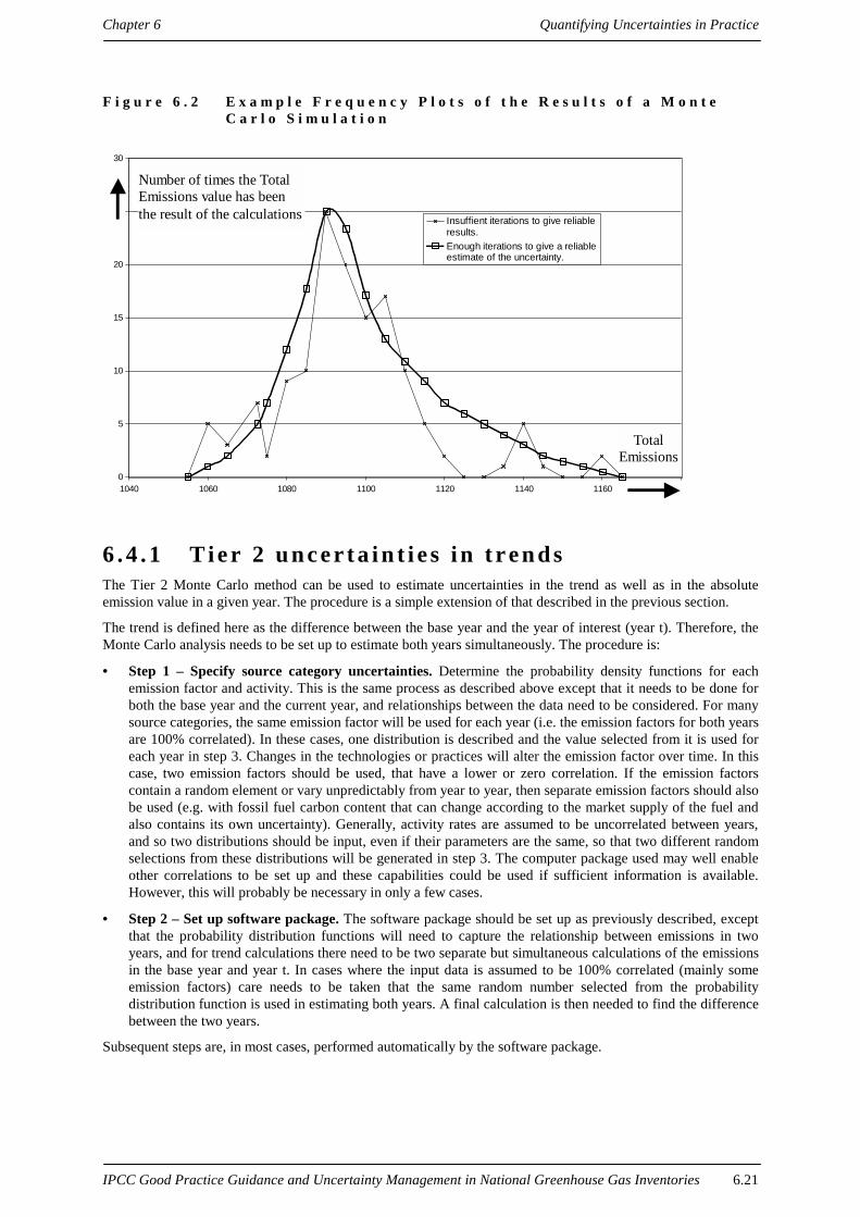
Chapter 6 Quantifying Uncertainties in Practice
IPCC Good Practice Guidance and Uncertainty Management in National Greenhouse Gas Inventories 6.21
F i g u r e 6 . 2 E x a m p l e F r e q u e n c y P l o t s o f t h e R e s u l t s o f a M o n t eC a r l o S i m u l a t i o n
0
5
10
15
20
30
1040 1060 1080 1100 1120 1140 1160
Insuffient iterations to give reliable results. Enough iterations to give a reliable estimate of the uncertainty.
Total Emissions
Number of times the Total Emissions value has been the result of the calculations
6 . 4 . 1 T i e r 2 u n c e r t a i n t i e s i n t r e n d sThe Tier 2 Monte Carlo method can be used to estimate uncertainties in the trend as well as in the absoluteemission value in a given year. The procedure is a simple extension of that described in the previous section.
The trend is defined here as the difference between the base year and the year of interest (year t). Therefore, theMonte Carlo analysis needs to be set up to estimate both years simultaneously. The procedure is:
• Step 1 – Specify source category uncertainties. Determine the probability density functions for eachemission factor and activity. This is the same process as described above except that it needs to be done forboth the base year and the current year, and relationships between the data need to be considered. For manysource categories, the same emission factor will be used for each year (i.e. the emission factors for both yearsare 100% correlated). In these cases, one distribution is described and the value selected from it is used foreach year in step 3. Changes in the technologies or practices will alter the emission factor over time. In thiscase, two emission factors should be used, that have a lower or zero correlation. If the emission factorscontain a random element or vary unpredictably from year to year, then separate emission factors should alsobe used (e.g. with fossil fuel carbon content that can change according to the market supply of the fuel andalso contains its own uncertainty). Generally, activity rates are assumed to be uncorrelated between years,and so two distributions should be input, even if their parameters are the same, so that two different randomselections from these distributions will be generated in step 3. The computer package used may well enableother correlations to be set up and these capabilities could be used if sufficient information is available.However, this will probably be necessary in only a few cases.
• Step 2 – Set up software package. The software package should be set up as previously described, exceptthat the probability distribution functions will need to capture the relationship between emissions in twoyears, and for trend calculations there need to be two separate but simultaneous calculations of the emissionsin the base year and year t. In cases where the input data is assumed to be 100% correlated (mainly someemission factors) care needs to be taken that the same random number selected from the probabilitydistribution function is used in estimating both years. A final calculation is then needed to find the differencebetween the two years.
Subsequent steps are, in most cases, performed automatically by the software package.

Quantifying uncertainties in Practice Chapter 6
IPCC Good Practice Guidance and Uncertainty Management in National Greenhouse Gas Inventories6.22
• Step 3 – Select random variables. The computer program will proceed as previously described, takingaccount of any correlation between probability density functions (PDF). Figure 6.3, below, shows thecalculation scheme for trend analysis
• Step 4 – Estimate Emissions. As in the previous description, the variables selected in Step 3 will be used toestimate the total emissions.
• Step 5 – Results. The emissions total calculated in step 4 is stored in a data file. The process then repeatsfrom step 3 until there is adequate convergence of the results. Considerations for this are the same asdescribed above. A range of results is estimated at the same time including total and sectoral emissions forthe base year, total and sectoral emissions for year t, and the differences (trends) between these for the totaland any sectors of interest.
F i g u r e 6 . 3 C a l c u l a t i o n S c h e m e f o r M o n t e C a r l o A n a l y s i s o f t h eA b s o l u t e E m i s s i o n s a n d t h e T r e n d o f a S i n g l e S o u r c eC a t e g o r y , E s t i m a t e d a s E m i s s i o n F a c t o r T i m e s a nA c t i v i t y R a t e
Source 1
Emission Factor 1
find pdf
Source 1
Activity data Base Year
find pdf
Source 1
Activity data Year t
find pdf
Select from
Select from
Select from
Trend =Emission Year t - Emissionin base year
Source 1
Activity data base year
find pdf
Source 1
Activity data year t
find pdf
Select from
Select from
Select from
EmissionBase year =
Emis. Factorx Activity
TrendEmission Year t
- Emissionin base year
Select from
Case where the emission factor is 100%correlated between base year and year t (e.g. the
same emission factor is used in each year and thereis no year to year variation expected)
Case where the emission factor is not correlatedbetween in base year and year t (e.g. emission factorfor coal where fuel varies from year to year or
where technologies change)
Source 1Emission factor 1
Year tfind pdf
Source 1Emission factor 1
Base Yearfind pdf
EmissionYear t =Emis. Factor xActivity
EmissionBase Year =Emis. Factorx Activity
EmissionYear t =Emis. Factorx Activity
6 . 4 . 2 R e p o r t i n g T i e r 2 u n c e r t a i n t y a n a l y s i sThe following data format is suitable for reporting the results of the Monte Carlo simulation for emissions bysource category, by fuel (where appropriate) and by greenhouse gas expressed as CO2 equivalent. In Table 6.2,the overall uncertainty in the national emissions trend appears at the foot of columns I and J. Inventory agenciesperforming a Tier 2 analysis should also report the results of a Tier 1 analysis using Table 6.1, as set out inSection 6.3.1, Comparison between tiers and choice of method.

IPCC Good Practice Guidance and Uncertainty management in National Greenhouse Gas Inventories6.23
TABLE 6.2
TIER 2 UNCERTAINTY REPORTING
A B C D E F G H I J
IPCC Sourcecategory
Gas Base yearemissions
Year temissions
Uncertainty in year t emissions as% of emissions in the category
Uncertainty introducedon national total inyear t
% change inemissionsbetween year tand base year
Range of likely % changebetween year t and base year
(Gg CO2equivalent)
(Gg CO2equivalent)
% below(2.5 percentile)
% above(97.5percentile)
(%) (%) Lower %(2.5percentile)
Upper %(97.5percentile)
e.g.1.A.1Energy IndustriesFuel 1
CO2
e.g.1.A.2Energy IndustriesFuel 2
CO2
Etc… …
Total

Quantifying uncertainties in Practice Chapter 6
IPCC Good Practice Guidance and Uncertainty Management in National Greenhouse Gas Inventories6.24
6 . 5 P R A C T I C A L C O N S I D E R A T I O N S I N U S I N GM O N T E C A R L O S I M U L A T I O N
Monte Carlo simulation requires that the analyst specify probability distributions for each model input for whichthe uncertainty is to be quantified. The assumption is that the simulation is a reasonable representation of the realworld. The probability distributions may be obtained by a variety of methods, including statistical analysis ofdata, or the elicitation of expert judgement. A key consideration is to develop the distributions for the inputs sothat they are all based upon the same underlying assumptions regarding averaging time, location, and otherconditioning factors relevant to the particular assessment (e.g. climatological conditions influencing agriculturalgreenhouse gas emissions). For this reason, one should not assume that an uncertainty distribution from anothercountry is directly applicable as an input to an inventory.
6 . 5 . 1 S p e c i f y i n g p r o b a b i l i t y d i s t r i b u t i o n s f o ri n v e n t o r y i n p u t s
Monte Carlo simulation requires identification of the model inputs for which probability distributions are to beassigned, and development of the corresponding probability distributions. Methods for developing distributionsbased upon elicitation of expert judgement have already been reviewed in this chapter. Methods for developingdistributions based upon statistical analysis of data are described and illustrated by Cullen and Frey (1999). Otheruseful references include Hahn and Shapiro (1967), Ang and Tang (1975), D’Agostino and Stephens (1986),Morgan and Henrion (1990), and USEPA (1996, 1997, 1999). Some examples of probabilistic analyses appliedto emission inventories are given by Frey et al. (1998) and Frey et al. (1999).
In order to use data as a basis for developing distributions, the first critical step is to determine if the data are arandom, representative sample, in the case of a sample from a population. Some key questions to ask regardingthe data include:
• Are the data representative of the variety of conditions pertaining to the emission or activity factors specificto national circumstances?
• Are the data a random sample?
• What is the averaging time associated with the data set, and is it the same as for the assessment (which willbe for annual emissions in a given year)?
If the data are a random, representative sample, then the distribution can be established directly using classicalstatistical techniques, even if the sample size is small. It may be necessary to convert data using an appropriateaveraging time. General advice on choosing probability density functions is provided in Annex 1, ConceptualBasis for Uncertainty Analysis, Section 2.5, Good Practice Guidance for Selecting a Probability DensityFunction.
In the ideal case, available data will represent an annual average for an emission factor or an annual total foractivity data. In this case, the data would represent a single sample from a population distribution of annualaverage values. The estimated standard deviation of the population would be an appropriate measure ofuncertainty in annual emissions. In other cases, the data may represent an exhaustive census of the sum of allactivity (e.g. total energy use for a particular fuel). In this case, information regarding errors in the measurementsor survey instruments would form a basis for assessing uncertainty. The range of uncertainty of activity datamight be bounded using independent methods or consistency checks. For example, fuel consumption data can becompared with estimates of production, including estimates of production via different methods.
In the case of a population sample, the most critical aspect to evaluate is whether the data are random andrepresentative of the population. If these conditions are met, classical statistical methods can be used to define thedistribution. If not, then some combination of data analysis and expert elicitation of distributions will be required.In the former case, Cullen and Frey (1999) suggest exploration of the data set using summary statistics andgraphics to evaluate essential features (e.g. central tendency, range of variation, skewness). The insights obtainedby examining the data, combined with knowledge of the processes that generated the data, should be consideredwhen selecting a mathematical or numerical representation of the distribution for input into the Monte Carlosimulation.

Chapter 6 Quantifying Uncertainties in Practice
IPCC Good Practice Guidance and Uncertainty Management in National Greenhouse Gas Inventories 6.25
Once a particular distribution is selected as a candidate for fitting to the data set, techniques such as ‘maximumlikelihood estimation5’ or the ‘method of matching moments6’ can be used to estimate the parameters of thedistribution. The goodness-of-fit of the distribution can be evaluated in numerous ways, including comparison ofthe fitted cumulative distribution function (CDF) with the original data set, probability plots, and goodness-of-fittests (e.g. Cullen and Frey, 1999). It is important that the selection of a parametric distribution to represent a dataset should be based not solely upon goodness-of-fit tests, but upon similarities in processes that generated thedata versus the theoretical basis for a distribution (e.g. Hahn and Shapiro, 1967).
If the data are averaged over less than one year, it may be necessary to extrapolate the uncertainty over the year.Consider an example in which the data set represents variability in daily average emissions measurements for aparticular source category. One approach, described in detail by Frey and Rhodes (1996), is to fit a parametricdistribution to the data set for daily variability, use a numerical technique known as bootstrap simulation toestimate uncertainty in the parameters of the distribution, and use Monte Carlo simulation to simulate randomisedannual averages of the emission factor. Using bootstrap simulation, the uncertainty in the sampling distributionfor the parameters for the fitted distribution can be simulated (e.g. Efron and Tibshirani, 1993; Frey and Rhodes,1996; Frey and Burmaster, 1999).
A simple form of bootstrap simulation works as follows: from the fitted distribution, a random synthetic data setof the same sample size as the original dataset is simulated using Monte Carlo simulation. The synthetic data setis referred to as a bootstrap sample. For the bootstrap sample, any statistic or parameter can be calculated, suchas a mean or parameters of a new distribution fitted to the synthetic data set. A statistic or parameter estimatedfrom a bootstrap sample is referred to as a bootstrap replicate of that statistic or parameter. This process is thenrepeated many times (typically 500 to 1,000), generating a corresponding number of bootstrap samples andduplicated statistics. The statistics will take on different values each time because the bootstrap samples arerandomised versions patterned after the original data set. Thus, this method is a numerical technique forestimating sampling distributions for any statistic for any type of distribution for which the statistic exists. Inessence, bootstrap simulation is a numerical technique for simulating random sampling error. The 500 to 1,000bootstrap samples imply a corresponding number of alternative plausible distributions from which the originaldata set could have been a random sample. For these alternative distributions, each of which reflects dailyvariability in the example, one can simulate a year’s worth of emissions estimates (i.e. 365 random samples ofdaily emissions summed to give an annual total or averaged to give an annual average emission factor), therebyyielding 500 to 1,000 estimates of annual mean or annual total emissions. The distribution of these estimates willdescribe uncertainty in the annual case based upon random sampling error. A key assumption in this example isthat there is no autocorrelation among the daily values, and that the daily values are representative of annualconditions – that there are for example no seasonal effects that the sample fails to capture.
6 . 5 . 2 H o w mu c h e f f o r t i s n e e d e d t o c h a r a c t e r i s eu n c e r t a i n t y i n a n i n v e n t o r y i n p u t ?
Ideally, the amount of effort devoted to characterising uncertainty in an inventory input should be proportional toits importance to the overall uncertainty assessment. It would not be a good use of limited resources to spendlarge amounts of time exhaustively collecting data and expert judgements for a source category that has littleeffect on overall uncertainty. Similarly, it would be a shortcoming of an assessment not to devote reasonableresources to quantifying uncertainty in inputs to which the overall uncertainty in the inventory is highly sensitive.Thus, many analysts who perform probabilistic simulation suggest an iterative approach to performing thesimulation. In the first iteration of an uncertainty analysis, preliminary assessments of uncertainty of inputs maybe made and propagated through the inventory solely for the purpose of making a preliminary identification ofwhat the main sources of uncertainty are. Methods for assessing the importance of each input are described inreferences such as Morgan and Henrion (1990), Frey and Cullen (1999), and others. An example of one relativelysimple technique is to calculate the correlation coefficient between the simulated numerical values of theinventory output distribution and the numerical values simulated for each input distribution. This correlationreflects the strength of the linear relationship between the two. The larger the magnitude of the correlation
5 The method of maximum likelihood selects as estimates the values of the parameters that maximise the likelihood (the jointprobability function or joint density function) of the observed sample.
6 The method of moments finds estimators of unknown parameters by equating corresponding sample and populationmoments. The method is easy to employ and provides consistent estimators. In many cases the method of moments estimatorsare biased (Wackerly, Mendenhall III and Scheaffer, 1996; pp. 395-397).
Quantifying uncertainties in Practice Chapter 6
IPCC Good Practice Guidance and Uncertainty Management in National Greenhouse Gas Inventories6.26
coefficient, the stronger is the relationship between uncertainty in the input and uncertainty in the output,indicating that the input should be considered as a ‘sensitive’ one. Many software packages will perform thesensitivity calculation automatically for the user and present them graphically.
After identifying the sensitive inputs, efforts can then be directed as appropriate to improve the estimate ofuncertainty for only those inputs. Then, the final uncertainty analysis can be performed with greater confidenceon the basis that important inputs have received proportionally greater attention than insensitive inputs.
Another point regarding iteration pertains to the longer-term aspects of performing uncertainty analyses. It can bedaunting to set up a Monte Carlo simulation for the first time. However, as the inventory agency gains experiencewith these analyses, the agency will likely find it easier to improve the analysis in the future. Monte Carloanalysis is typically a learning process for all involved, because it motivates critical and important questionsregarding the basis for and quality of an emission inventory. Thus, over time, Monte Carlo simulation will help indeciding where to focus data collection activities that will result in improved confidence regarding the inventory.
6 . 5 . 3 C h o o s i n g a s i mu l a t i o n t e c h n i q u e a n d as i mu l a t i o n s a mp l e s i ze
There are several commercially available software tools that can be used to perform Monte Carlo simulation.Examples of these include Crystal Ball, @Risk, Analytica, and Mathematica. The first two are add-ins forcommonly used spreadsheet programs. Many software tools offer an option of different sampling methods,including random Monte Carlo simulation and variations of Latin Hypercube Sampling (LHS). LHS can produce‘smoother’ looking model output distributions for sample sizes of only a few hundred samples. The disadvantageof using LHS is that one must decide ahead of time how many iterations to use. This is because two or more LHSsimulations cannot be combined since they will use overlapping strata, leading to difficulties in interpretingresults. In some cases, LHS can yield underestimates of the higher moments of probability distributions, since thestratification method also can preclude clustering of very high or low values as can occur in random data sets.The overall suggestion is to use random Monte Carlo simulation as the default method, because it will giveflexibility to continue a random simulation to larger and larger simulation sample sizes if necessary until themodel output distribution converges. Cullen and Frey (1999) provide more information on the comparison ofLHS and Monte Carlo simulation (pp. 207-213).
6 . 5 . 4 D e p e n d e n c e a n d c o r r e l a t i o n a mo n gi n v e n t o r y i n p u t s
A key issue often considered by analysts when setting up a probabilistic analysis is whether there aredependencies or correlations among model inputs. Ideally, it is preferable to define the model so that the inputsare as statistically independent of each other as possible. Rather than to try to estimate activity data for many sub-categories for which data are derived at least in part by differences, it may be better to assign uncertainties tobetter known aggregate measures of activity. For example, residential fuel use might be estimated as thedifference between total consumption and usage in the transportation, industrial, and commercial sectors. In thiscase, the estimate of uncertainty in residential fuel use is negatively correlated with the uncertainties in fuel use inthe other sub-categories, and may even be very large compared to the uncertainty in total consumption. Thus,rather than try to estimate uncertainties separately for each sub-category, it would be more practical to estimateuncertainty for total consumption, for which good estimates and cross-checks may be available.
6 . 5 . 5 D o e s c o r r e l a t i o n ma t t e r ?An important point to remember is that dependencies, even if they exist, may not be important to the assessmentof uncertainties. Dependencies among inputs will matter only if the dependencies exist between two inputs towhich the uncertainty in the inventory is sensitive and if the dependencies are sufficiently strong. In contrast,weak dependencies among inputs, or strong dependencies among inputs to which the uncertainty in the inventoryis insensitive, will be of relatively little consequence to the analysis.

Chapter 6 Quantifying Uncertainties in Practice
IPCC Good Practice Guidance and Uncertainty Management in National Greenhouse Gas Inventories 6.27
6 . 5 . 6 S o me me t h o d s f o r d e a l i n g w i t h d e p e n d e n c i e so r c o r r e l a t i o n
When dependencies among inputs are judged to be of importance, then a variety of techniques can be consideredfor incorporating them into the analysis. Examples include: (i) modelling the dependence explicitly; (ii)stratifying or aggregating the source categories to minimise the effect of the dependencies; (iii) simulatingcorrelation using restricted pairing methods (that are included in many software packages); (iv) use of resamplingtechniques in cases where multivariate datasets are available; (v) considering bounding or sensitivity cases (e.g.one case assuming independence and another case assuming complete positive correlation). More discussion andexamples of these types of methods are given in Cullen and Frey (1999), Morgan and Henrion (1990), andUSEPA (1996). These documents also contain reference lists with citations to relevant literature.
6 . 5 . 7 S p e c i f y i n g c o r r e l a t i o n i n i n v e n t o r y i n p u t sMany software packages allow specification of a correlation between model inputs (e.g. Iman and Conover,1982). In some cases, these packages may offer this feature only with LHS, while in others it may be availablealso in conjunction with random Monte Carlo simulation. There is a detail regarding these methods that advancedusers will want to note, which is that these software tools can induce a rank correlation between any two or moredistributions, but not a sample correlation. However, there are methods that one can use to specify samplecorrelation in some types of distributions, such as for multivariate normal distributions (see Morgan and Henrion,1990 or Cullen and Frey, 1999 for examples).
6 . 5 . 8 A n a l y s i n g i n v e n t o r y o u t p u t sMany software packages allow the user to display probability density functions (PDF), cumulative distributionfunctions (CDF) and provide output of summary statistics for a given model input. Typically, the CDF willappear to be a smoother curve than the PDF for any given case. Furthermore, the CDF allows for quantitativeinterpretations of the median, 95 percent confidence interval, or any other percentile of the distribution. Thus, forpractical purposes, the CDF is often the most useful representation of the model output. The PDF is useful forobtaining qualitative insights regarding the output, such as whether it is positively skewed.
6 . 5 . 9 E n c o u r a g e me n t o f u s e o f a p p r o p r i a t et e c h n i q u e s
The guidance offered here is not meant to preclude the use of improved methods as they become available.Furthermore, this document does not cover all situations that may be faced by an analyst. Therefore, theinventory agency is encouraged to refer to the references cited below for additional suggestions on how toperform uncertainty analyses.
6 . 6 C O N C L U S I O NThe methods described in this chapter should enable inventory agencies to estimate and report the uncertainty intotal emissions in any year, and the uncertainty in the trend between years, together with the contribution thateach source category makes to these overall uncertainties. This information should help prioritise efforts toimprove the precision of inventories in future, and can show how the overall and trend uncertainties respond asthe uncertainties in individual source categories are reduced.

Quantifying uncertainties in Practice Chapter 6
IPCC Good Practice Guidance and Uncertainty Management in National Greenhouse Gas Inventories6.28
A P P E N D I X 6 A . 1D E R I V A T I ON OF T HE F OR M U L A E I N T A B L E 6 . 1( T I E R 1 )
EXPLANATION OF THE VARIABLES
Cx = Value of an entry in column C and row x
n = number of emission categories (rows)
∑ iC = Sum over all emissions categories (rows) of the inventory from i=1 to i=n
COLUMN A-F
Input data
COLUMN G
Combined uncertainty using error propagation equation
2x
2xx FEG +=
COLUMN H
Combined uncertainty as a percentage of the total emissions in year t.
∑•
=i
xxx D
DGH
The total in column H (total emission uncertainty) is obtained using the error propagation equation:
( )∑=
∑
∑
•
∑
=x
2x
xx
x
2x
2
xx
HD
HD
HcolumnofTotal
COLUMN I
Entries in column I show how the difference in emissions between the base year and the year t changes inresponse to a 1% increase in emissions of source category x emissions in the base year and year t. This shows thesensitivity of the trend in emissions to a systematic uncertainty in the emission estimate – i.e. one that iscorrelated between the base year and year t. This sensitivity is described as type A sensitivity.

Chapter 6 Quantifying Uncertainties in Practice
IPCC Good Practice Guidance and Uncertainty Management in National Greenhouse Gas Inventories 6.29
Ix = percentage trend if source category x is increased by 1% in both years – percentage trend without increase
100C
CD100
)CC(0.01)CC(0.01DD0.01
i
ii
ix
ixix •∑
∑ ∑−−•
∑+•∑ ∑+•−+•
=
COLUMN J
Entries in column J show how the difference in emissions between the base year and year t changes in response toa 1% increase in the emissions of source category x in year t only. This shows the sensitivity of the trend inemissions to random uncertainty error in the emissions estimate – i.e. one that is not correlated between the baseyear and year Y. This sensitivity is described as type B sensitivity.
Jx = percentage trend if source category x is increased by 1% in year t – percentage trend without increase
∑=
•∑
∑ ∑−−•
∑∑ ∑−+•
=
i
x
i
ii
i
iix
CD
100C
CD100
CCDD0.01
COLUMN K
Under the assumption that the same emission factor is used in both years and the actual emission factors are fullycorrelated, the % error introduced by it is equal in both years. Therefore the formula for the uncertaintyintroduced on the trend by the emission factor is:
xx
x
FIfactoremission ofy uncertaint A y sensitivitK
•=•=
In case no correlation between emission factors is assumed, sensitivity B should be used and the result needs tobe increased by √2 for the reason given below in the main derivation for column L:
2FJ
2factoremission ofy uncertaint By sensitivitK
xx
x
••=
••=
COLUMN L
The trend is the difference between the emissions in the base year and in the year t. Therefore the uncertainty ofthe activity data of the base year and t has to be taken into account. The two uncertainties combined using theerror propagation equation and the assumption that the uncertainty is the same in the base year and year t is:
( ) ( )( )
2E
2year t) data,(activity y uncertaint
year t) data,(activity y uncertaintyear) base data,(activity y uncertaint
x
2
22
•=
•≈
+=
Since activity data in both years are assumed to be independent, column L equals:
Lx = sensitivity B • combined uncertainty of activity data of both years
2EJ xx ••=

Quantifying uncertainties in Practice Chapter 6
IPCC Good Practice Guidance and Uncertainty Management in National Greenhouse Gas Inventories6.30
In case correlation between activity data is assumed, sensitivity A should be used and the √2 factor does notapply.
xxx EIL •=
COLUMN M
In column M figures the combined uncertainty introduced on the trend by the uncertainty in the activity data andthe emissions factor.
2x
2xx LKM +=
The entries Mi in column M are combined to obtain the total uncertainty of the trend using the error propagationequation as follows:
( )2
n2
22
1
xxx
x
2x
2
xxx
M...MM)C(D
M)C(D
Mcolumn of Total +++=∑ −
∑
•
∑ −
=

IPCC Good Practice Guidance and Uncertainty Management in National Greenhouse Gas Inventories6.31
A P P E N D I X 6 A . 2T I E R 1 U N C E R T A I N T Y C A L C U L A T I O N E XA M P L EThe following spreadsheet shows an example calculation for the national greenhouse gas inventory of the United Kingdom.
TABLE 6.3
TIER 1 UNCERTAINTY CALCULATION AND REPORTING EXAMPLE
A B C D E F G H I J K L MIPCC Source Category Gas Base year
emissions1990
Year temissions
1997
Activitydata
uncertainty
Emissionfactor
uncertainty
Combineduncertainty
Combineduncertainty
as % oftotal national
emissionsin year t
Type A sensitivity Type B sensitivity Uncertainty intrend in national
emissionsintroduced by
emission factoruncertainty
Uncertainty intrend in national
emissionsintroduced byactivity datauncertainty
Uncertaintyintroduced into
the trend in totalnational emissions
Gg CO2equivalent
Gg CO2equivalent
% % % % % % % % %
1A Coal CO2 238 218 142 266 1.2 6 6.1 1.2 -0.0966 0.1840 -0.58 0.31 0.661A Oil CO2 208 684 196 161 1 2 2.2 0.6 0.0076 0.2538 0.02 0.36 0.361A Natural Gas CO2 111 052 181 691 2 1 2.2 0.6 0.1039 0.2351 0.10 0.66 0.671A Other (waste) CO2 138 741 7 20 21.2 0.0 0.0008 0.0010 0.02 0.01 0.021B Solid Fuel Transformation CO2 2 573 1 566 1.2 6 6.1 0.0 -0.0010 0.0020 -0.01 0.00 0.011B Oil & Natural Gas CO2 8 908 6 265 14 14.0 0.1 -0.0024 0.0081 -0.03 0.00 0.032A1 Cement Production CO2 6 693 6 157 1 2 2.2 0.0 0.0001 0.0080 0.00 0.01 0.012A2 Lime Production CO2 1 192 1 703 1 5 5.1 0.0 0.0008 0.0022 0.00 0.00 0.012A3 Limestone & Dolomite use CO2 1 369 1 551 1 5 5.1 0.0 0.0004 0.0020 0.00 0.00 0.002A4 Soda Ash Use CO2 116 120 15 2 15.1 0.0 0.0000 0.0002 0.00 0.00 0.002B Ammonia Production CO2 1 358 814 5 5.0 0.0 -0.0005 0.0011 0.00 0.00 0.002C1 Iron&Steel Production CO2 3 210 1 495 1.2 6 6.1 0.0 -0.0019 0.0019 -0.01 0.00 0.015D Land Use Change & Forestry CO2 31 965 27 075 5 54 54.2 2.1 -0.0027 0.0350 -0.14 0.25 0.296C MSW Incineration CO2 660 29 7 20 21.2 0.0 -0.0007 0.0000 -0.01 0.00 0.01
CO2 Total 616 137 567 634
1A All Fuel CH4 2 507 1 975 1.2 50 50.0 0.1 -0.0004 0.0026 -0.02 0.00 0.021B1 Coal Mining CH4 17 188 6 687 1 13 13.0 0.1 -0.0116 0.0087 -0.15 0.01 0.15
Solid Fuel Transformation CH4 215 173 6 50 50.4 0.0 0.0000 0.0002 0.00 0.00 0.001B2 Natural Gas Transmission CH4 8 103 7 301 2 15 15.1 0.2 -0.0001 0.0094 0.00 0.03 0.03
Offshore Oil& Gas CH4 2 402 1 957 10 26 27.9 0.1 -0.0003 0.0025 -0.01 0.04 0.042C Iron & Steel Production CH4 16 13 1.2 50 50.0 0.0 0.0000 0.0000 0.00 0.00 0.004A Enteric Fermentation CH4 19 177 18 752 1 20 20.0 0.5 0.0016 0.0243 0.03 0.03 0.054B Manure Management CH4 2 338 2 325 1 30 30.0 0.1 0.0003 0.0030 0.01 0.00 0.014F Field Burning CH4 266 0 25 50 55.9 0.0 -0.0003 0.0000 -0.02 0.00 0.026A Solid Waste Disposal CH4 23 457 17 346 15 46 48.4 1.2 -0.0052 0.0224 -0.24 0.48 0.536B Wastewater Handling CH4 701 726 15 48 50.3 0.1 0.0001 0.0009 0.01 0.02 0.026C Waste Incineration CH4 1 1 7 50 50.5 0.0 0.0000 0.0000 0.00 0.00 0.00
CH4 total 76 371 57 257

IPCC Good Practice Guidance and Uncertainty Management in National Greenhouse Gas Inventories6.32
TABLE 6.3
TIER 1 UNCERTAINTY CALCULATION AND REPORTING EXAMPLE
A B C D E F G H I J K L MIPCC Source Category Gas Base year
emissions1990
Year temissions
1997
Activitydata
uncertainty
Emissionfactor
uncertainty
Combineduncertainty
Combineduncertainty
as % oftotal national
emissionsin year t
Type A sensitivity Type B sensitivity Uncertainty intrend in national
emissionsintroduced by
emission factoruncertainty
Uncertainty intrend in national
emissionsintroduced byactivity datauncertainty
Uncertaintyintroduced into
the trend in totalnational emissions
Gg CO2equivalent
Gg CO2equivalent
% % % % % % % % %
1A2&1A4&1A5
Other Combustion N2O 3 865 3 562 1.2 195 195.0 1.0 0.0001 0.0046 0.01 0.01 0.01
1A3 Transport N2O 1 300 3 645 1.4 170 170.0 0.9 0.0032 0.0047 0.54 0.01 0.541B2 Oil & Natural Gas N2O 3 2 10 110 110.5 0.0 0.0000 0.0000 0.00 0.00 0.002B Adipic Acid Production N2O 25 136 17 766 0.5 15 15.0 0.4 -0.0067 0.0230 -0.10 0.02 0.102B Nitric Acid Production N2O 4 383 3 723 10 230 230.2 1.2 -0.0004 0.0048 -0.08 0.07 0.114B Manure Management N2O 1 583 1 559 1 509a 509.0 1.1 0.0002 0.0020 0.08 0.00 0.084D Agricultural Soils N2O 29 472 29 098 1 509 509.0 21.0 0.0029 0.0376 1.47 0.05 1.474F Field Burning N2O 78 0 10 230 230.2 0.0 -0.0001 0.0000 -0.02 0.00 0.026B Wastewater Handling N2O 153 157 1 100 100.0 0.0 0.0000 0.0002 0.00 0.00 0.006C Waste Incineration N2O 115 11 7 230 230.1 0.0 -0.0001 0.0000 -0.03 0.00 0.03
N2O Total 66 089 59 525
2 Industrial Processes HFC 11 374 18 447 2 25 25.1 0.7 0.0104 0.0239 0.26 0.07 0.273 Industrial Processes PFC 2 281 661 5 19 19.6 0.0 -0.0018 0.0009 -0.03 0.01 0.044 Industrial Processes SF6 724 1 170 10 8 12.8 0.0 0.0007 0.0015 0.01 0.02 0.02
Halocarbon & SF6 Total
Total Emissions GWPweighted total
772 976 704 693
Total Uncertainties Overall uncertainty in the year (%) 21.3 Trend uncertainty (%) 2.0
a Uncertainty estimated from lognormal distribution used in Monte Carlo simulation. I.e. (97.5 percentile-mean)/mean *100.
Chapter 6 Quantifying Uncertainties in Practice
IPCC Good Practice Guidance and Uncertainty Management in National Greenhouse Gas Inventories 6.33
R E F E R E N C E SAng, A.H.S. and W.H. Tang (1975). Probability Concepts in Engineering Planning and Design, Volume 1. JohnWiley and Sons, New York.
Cullen, A.C. and H.C. Frey (1999). Probabilistic Techniques in Exposure and Risk Assessment: A Handbook forDealing with Variability and Uncertainty in Models and Inputs. Plenum Press, New York.
D’Agostino, R.B. and M.A. Stephens (1986). Goodness of Fit Techniques. Marcel Dekker, New York.
Efron, B. and Tibshirani, R.J. (1993). An Introduction to the Bootstrap. Chapman and Hall, New York.
Eggleston, S. et al. (1998). Treatment of Uncertainties for National Greenhouse Gas Emissions. Report AEAT2688-1 for DETR Global Atmosphere Division, AEA Technology, Culham, UK.
Fishman G.S. (1996). Monte Carlo: Concepts, Algorithms, and Applications. Springer-Verlag, New York.
Frey, H.C. and D.E. Burmaster (1999). ‘Methods for Characterization of Variability and Uncertainty:Comparison of Bootstrap Simulation and Likelihood-Based Approaches’. Risk Analysis, 19(1): 109-129.
Frey, H.C. and D.S. Rhodes (1996). ‘Characterizing, Simulating, and Analyzing Variability and Uncertainty: AnIllustration of Methods Using an Air Toxics Emissions Example’. Human and Ecological Risk Assessment, 2(4),pp. 762-797.
Frey, H.C., Bharvirkar, R., Thompson, R. and Bromberg, S. (1998). ‘Quantification of Variability andUncertainty in Emission Factors and Inventories’. Proceedings of Conference on the Emission Inventory, Air &Waste Management Association, Pittsburgh, PA, USA.
Frey, H.C., Bharvirkar, R. and Zheng, J. (1999). Quantitative Analysis of Variability and Uncertainty inEmissions Estimation, Final Report. Prepared by North Carolina State University for U.S. EnvironmentalProtection Agency, Research Triangle Park, North Carolina, USA, July 1999. Available at www4.ncsu.edu/~frey/
Hahn, G. J. and Shapiro, S. S. (1967). Statistical Models in Engineering, John Wiley and Sons, New York.
Hora, S.C., and R.L. Iman (1989). ‘Expert opinion in risk analysis: The NUREG-1150 methodology’. NuclearScience and Engineering, 102, pp. 323-331.
Iman, R. L. and Conover, W. J. (1982). ‘A Distribution-Free Approach to Inducing Rank Correlation AmongInput Variables’. Communications in Statistics, B11(3), pp. 311-334.
McCann, T.J. & Associates and Nosal, M. (1994). Report To Environment Canada Regarding Uncertainties InGreenhouse Gas Emission Estimates. Calgary, Canada.
Merkhofer, M.W. (1987). ‘Quantifying judgmental uncertainty: methodology, experiences, and insights’. IEEETransactions on Systems, Man, and Cybernetics, 17(5), pp. 741-752.
Morgan, M.G. and M. Henrion (1990). Uncertainty: A Guide to Dealing with Uncertainty in Quantitative Riskand Policy Analysis. Cambridge University Press, New York.
NCRP (National Council on Radiation Protection and Measurements) (1996). A Guide for Uncertainty Analysisin Dose and Risk Assessments Related to Environmental Contamination. NCRP Commentary No. 14, Bethesda,MD, USA.
Robinson, J.R. (1989). ‘On Uncertainty in the Computation of Global Emissions for Biomass Burning’. ClimaticChange, 14, pp. 243-262.
Spetzler, C.S., and von Holstein, S. (1975). ‘Probability encoding in decision analysis’. Management Science,22(3), pp. 340-358.
USEPA (1996). Summary Report for the Workshop on Monte Carlo Analysis. EPA/630/R-96/010, RiskAssessment Forum, U.S. Environmental Protection Agency, Washington, DC, USA.
USEPA (1997). Guiding Principles for Monte Carlo Analysis. EPA/630/R-97/001, Office of Research andDevelopment, U.S. Environmental Protection Agency, Washington, DC, USA, March 1997. Available on WorldWide Web at: http://www.epa.gov/ncea/mcpolicy.htm.
USEPA (1999). Report of the Workshop on Selecting Input Distributions For Probabilistic Assessments.EPA/630/R-98/004, Office of Research and Development, U.S. Environmental Protection Agency, Washington,DC, January 1999. Available on World Wide Web at: http://www.epa.gov/ncea/input.htm.

Quantifying uncertainties in Practice Chapter 6
IPCC Good Practice Guidance and Uncertainty Management in National Greenhouse Gas Inventories6.34
Wackerly, D. D., Mendenhall III, W. and Scheaffer, R. L. (1996). Mathematical Statistics with Applications.Duxbury Press, USA.

Chapter 7 Methodological Choice and Recalculation
IPCC Good Practice Guidance and Uncertainty Management in National Greenhouse Gas Inventories 7.1
7
METHODOLOGICAL CHOICE ANDRECALCULATION

7.2 IPCC Good Practice Guidance and Uncertainty Management in National Greenhouse Gas Inventories
Methodological Choice and Recalculation Chapter 7
CO-CHAIRS, EDITORS AND EXPERTS
Co-chairs of the Expert Meeting on Cross-sectoral Methodologies forUncertainty Estimation and Inventory QualityTaka Hiraishi (Japan) and Buruhani Nyenzi (Tanzania)
REVIEW EDITOR
Buruhani Nyenzi (Tanzania)
Expert Group: Methodological Choice and RecalculationCO-CHAIRS
Dina Kruger (USA) and Bojan Rode (Slovenia)
AUTHORS OF BACKGROUND PAPERS
Kristin Rypdal (Norway), Ketil Flugsrud (Norway), and William Irving (USA)
CONTRIBUTORS
Roberto Acosta (UNFCCC Secretariat), William Ageymang-Bonsu (Ghana), Simon Bentley (Australia), MarceloFernandez (Chile), Pavel Fott (Czech Republic), Jorge Gasca (Mexico), Anke Herold (Germany), Taka Hiraishi(Japan), Robert Hoppaus (IPCC-NGGIP/TSU), William Irving (USA), Natalja Kohv (Estonia), Nils Lindth(Sweden), Thomas Martinsen (IPCC/OECD), Pauline McNamara (Switzerland), Alexander Nakhutin (RussianFederation), Buruhani Nyenzi (Tanzania), Riitta Pipatti (Finland), Kristin Rypdal (Norway), and Geoff Salway(UK)
Chapter 7 Methodological Choice and Recalculation
IPCC Good Practice Guidance and Uncertainty Management in National Greenhouse Gas Inventories 7.3
C o n t e n t s
7 METHODOLOGICAL CHOICE AND RECALCULATION
7.1 INTRODUCTION.................................................................................................................................7.4
7.2 DETERMINING NATIONAL KEY SOURCE CATEGORIES...........................................................7.5
7.2.1 Quantitative approaches to identify key source categories ........................................................7.5
7.2.2 Qualitative approaches to identify key source categories ........................................................7.13
7.2.3 Application of results...............................................................................................................7.14
7.2.4 Reporting and documentation ..................................................................................................7.16
7.3 RECALCULATIONS..........................................................................................................................7.17
7.3.1 Reasons for recalculations .......................................................................................................7.17
7.3.2 Approaches to recalculations ...................................................................................................7.18
7.3.3 Documentation.........................................................................................................................7.21
APPENDIX 7A.1 EXAMPLE OF TIER 1 KEY SOURCE CATEGORY IDENTIFICATION ..............7.22
REFERENCES ............................................................................................................................................7.26
F i g u r e s
Figure 7.1 Decision Tree to Identify Key Source Categories............................................................7.7
Figure 7.2 Cumulative Fraction of Uncertainty by Cumulative Fraction of Total Emissions .........7.11
Figure 7.3 Cumulative Fraction of Trend Uncertainty by Cumulative Fraction ofTotal Trend Assessment.................................................................................................7.11
Figure 7.4 Decision Tree to Choose a Good Practice Method ........................................................7.15
T a b l e s
Table 7.1 Suggested IPCC Source Categories .................................................................................7.6
Table 7.2 Spreadsheet for the Tier 1 Analysis – Level Assessment.................................................7.8
Table 7.3 Spreadsheet for the Tier 1 Analysis – Trend Assessment ..............................................7.10
Table 7.4 Source Category Analysis Summary..............................................................................7.16
Table 7.5 Summary of Approaches to Recalculations ...................................................................7.19
Table 7.A1 Tier 1 Analysis – Level Assessment (US inventory)......................................................7.23
Table 7.A2 Tier 1 Analysis – Trend Assessment (US inventory) .....................................................7.24
Table 7.A3 Source Category Analysis Summary (US inventory) .....................................................7.25

7.4 IPCC Good Practice Guidance and Uncertainty Management in National Greenhouse Gas Inventories
Methodological Choice and Recalculation Chapter 7
7 METHODOLOGICAL CHOICE ANDRECALCULATION
7 . 1 I N T R O D U C T I O N This chapter addresses two cross-cutting issues in inventory preparation: (i) how to identify key source categoriesin the national inventory, and (ii) how to systematically manage methodological change over time and ensure thattrends in national emissions are consistently estimated.
Methodological choice for individual source categories is important in managing overall inventory uncertainty.Generally, inventory uncertainty is lower when emissions are estimated using the most rigorous methods, but dueto finite resources, this may not be feasible for every source category. It is good practice to identify those sourcecategories that have the greatest contribution to overall inventory uncertainty in order to make the most efficientuse of available resources. By identifying these key source categories in the national inventory, inventoryagencies can prioritise their efforts and improve their overall estimates. Such a process will lead to improvedinventory quality, as well as greater confidence in the emissions estimates that are developed. It is good practicefor each inventory agency to identify its national key source categories in a systematic and objective manner.
A key source category is one that is prioritised within the national inventory system because its estimate has asignificant influence on a country’s total inventory of direct greenhouse gases in terms of the absolute level ofemissions, the trend in emissions, or both.
Any inventory agency that has prepared an emissions inventory will be able to identify key source categories interms of their contribution to the absolute level of national emissions. For those inventory agencies that haveprepared a time series, the quantitative determination of key source categories should include evaluation of boththe absolute level and the trend in emissions. Evaluating only the influence of a source category on the overalllevel of emissions provides limited information about why the source category is key. Some key sourcecategories may not be identified if the influence of their trend is not taken into account.
The quantitative approaches to determine key source categories are described in Section 7.2.1, QuantitativeApproaches to Identify Key Source Categories. Both a basic Tier 1 approach and a Tier 2 approach, whichaccounts for uncertainty, are described. In addition to making a quantitative determination of key sourcecategories, it is good practice to consider qualitative criteria. These qualitative criteria include high uncertainty,mitigation, significant anticipated changes in future emission levels, and significant differences between theestimate and what would be expected using an IPCC default method or factor. The application of these criteria isdescribed in more detail in Section 7.2.2, Qualitative Approaches to Identify Key Source Categories. The ways inwhich key source categories are to be managed within the inventory are also described along with references toother relevant sections of this report.
Inventory agencies will, from time to time, have good reason to change or refine the methods used to estimateemissions from particular source categories. Such changes may be made, for example, in order to improve theestimates of key source categories. These changes must be accompanied by a recalculation of previouslyprepared estimates in order to ensure that the reported emission trend is reliable. As far as possible, the timeseries should be recalculated using the same method in all years. In some cases, however, the same data sourcesfor all years will not be available. Guidance on how to recalculate emissions to ensure consistency in the trend insituations where the same method cannot be used in every year is described in Section 7.3, Recalculations.

Chapter 7 Methodological Choice and Recalculation
IPCC Good Practice Guidance and Uncertainty Management in National Greenhouse Gas Inventories 7.5
7 . 2 D E T E R M I N I N G N A T I O N A L K E Y S O U R C EC A T E G O R I E S
In each country’s national inventory, certain source categories are particularly significant in terms of theircontribution to the overall uncertainty of the inventory. It is important to identify these key source categories sothat the resources available for inventory preparation may be prioritised and the best possible estimates preparedfor the most significant source categories.
The results of the key source category determination will be most useful if the analysis is done at the appropriatelevel of detail.
Table 7.1, Suggested IPCC Source Categories, lists the source categories that should be analysed, and identifiesspecial considerations related to the analysis, where relevant. For example, the combustion of fossil fuels is alarge emission source category that can be broken down into sub-source categories, and even to the level ofindividual plants or boilers. The following guidance describes good practice in determining the appropriate levelof analysis to identify key source categories:
• The analysis should be performed at the level of IPCC source categories (i.e. at the level at which the IPCCmethods are described). The analysis should be performed using CO2-equivalent emissions calculated usingthe global warming potentials (GWPs) specified in the Guidelines for the preparation of nationalcommunications by Parties included in Annex I to the Convention, Part I: UNFCCC reporting guidelines onannual inventories (UNFCCC Guidelines).
• Each greenhouse gas emitted from a single source category should be considered separately, unless there arespecific methodological reasons for treating gases collectively. For example, carbon dioxide (CO2), methane(CH4) and nitrous oxide (N2O) are emitted from mobile sources. The key source category evaluation shouldbe performed for each of these gases separately because the methods, emission factors and relateduncertainties differ for each gas. In contrast, a collective evaluation of hydrofluorocarbons (HFCs) andperfluorocarbons (PFCs) may be appropriate for some source categories, such as emissions from substitutesfor Ozone Depleting Substances (ODS substitutes).
• Source categories that use the same emission factors based on common assumptions should be aggregatedbefore analysis. This approach can also help deal with cross-correlations between source categories in theuncertainty analysis, as explained in Chapter 6, Quantifying Uncertainties in Practice, Section 6.3.3, Tier1Aggregation and Reporting. The same pattern of aggregation should be used both to quantify uncertaintiesand to identify key source categories unless the associated activity data uncertainties are very different.
Finally, for each key source category, the inventory agency should determine if certain sub-source categories areparticularly significant (i.e. represent a significant share of the emissions). In the case of CH4 emissions fromenteric fermentation in domestic livestock, for example, emissions from particular species (e.g. cattle, buffalo orsheep) are likely to represent the major share of emissions. This also applies to industrial sources where a fewlarger plants account for most of the emissions of that source category. It may be appropriate to focus effortstowards methodological improvements on these most significant sub-source categories.
7 . 2 . 1 Q u a n t i t a t i v e a p p r o a c h e s t o i d e n t i f y ke ys o u r c e c a t e g o r i e s
It is good practice for each inventory agency to identify its national key source categories in a systematic andobjective manner, by performing a quantitative analysis of the relationships between the level and the trend ofeach source category’s emissions and total national emissions.
The decision tree in Figure 7.1, Decision Tree to Identify Key Source Categories, illustrates how inventoryagencies can determine which approach to use for the identification of key source categories. Any inventoryagency that has developed an emissions inventory will be able to perform the Tier 1 Level Assessment andidentify the source categories whose level has a significant effect on total national emissions. Those inventoryagencies that have developed emissions inventories for more than one year will also be able to perform the Tier 1Trend Assessment and identify sources that are key because of their contribution to the total trend of nationalemissions. Both assessments are described in Section 7.2.1.1, Tier 1 Method to Identify Key Source Categories.

7.6 IPCC Good Practice Guidance and Uncertainty Management in National Greenhouse Gas Inventories
Methodological Choice and Recalculation Chapter 7
TABLE 7.1SUGGESTED IPCC SOURCE CATEGORIES a,b
Source Categories to be Assessed in Key Source CategoryAnalysis
Special Considerations
ENERGY CO2 Emissions from Stationary Combustion Disaggregate to the level where emission factors are distinguished. In
most inventories, this will be the main fuel types. If emission factors aredetermined independently for some sub-source categories, these shouldbe distinguished in the analysis.
Non-CO2 Emissions from Stationary Combustion Assess CH4 and N2O separately. Mobile Combustion: Road Vehicles Assess CO2, CH4 and N2O separately. Mobile Combustion: Water-borne Navigation Assess CO2, CH4 and N2O separately. Mobile Combustion: Aircraft Assess CO2, CH4 and N2O separately. Fugitive Emissions from Coal Mining and Handling If this source is key, it is likely that underground mining will be the most
significant sub-source category. Fugitive Emissions from Oil and Gas Operations This source category comprises several sub-source categories which may
be significant. Inventory agencies should assess this source category, if itis key, to determine which sub-source categories are most important.
INDUSTRIAL PROCESSES
CO2 Emissions from Cement Production CO2 Emissions from Lime Production CO2 Emissions from the Iron and Steel Industry N2O Emissions from Adipic Acid and Nitric Acid Production Assess adipic acid and nitric acid separately. PFC Emissions from Aluminium Production Sulfur hexafluoride (SF6) from Magnesium Production SF6 Emissions from Electrical Equipment SF6 Emissions from Other Sources of SF6
SF6 Emissions from Production of SF6
PFC, HFC, SF6 Emissions from Semiconductor Manufacturing Assess emissions from all compounds jointly on a GWP-weighted basis,since they are all used in similar fashions in the process.
Emissions from Substitutes for Ozone Depleting Substances (ODSSubstitutes)
Assess emissions from all HFCs and PFCs used as substitutes for ODSjointly on a GWP-weighted basis, given the importance of having aconsistent method for all ODS sources.
HFC-23 Emissions from HCFC-22 ManufactureAGRICULTURE
CH4 Emissions from Enteric Fermentation in Domestic Livestock If this source category is key, it is likely that cattle, buffalo and sheepwill be the most significant sub-source categories.
CH4 Emissions from Manure Management If this source category is key, it is likely that cattle and swine will be themost significant sub-source categories.
N2O Emissions from Manure Management CH4 and N2O Emissions from Savanna Burning Assess CH4 and N2O separately. CH4 and N2O Emissions from Agricultural Residue Burning Assess CH4 and N2O separately. Direct N2O Emissions from Agricultural Soils Indirect N2O Emissions from Nitrogen Used in Agriculture CH4 Emissions from Rice ProductionWASTE
CH4 Emissions from Solid Waste Disposal Sites Emissions from Wastewater Handling Assess CH4 and N2O separately. Emissions from Waste Incineration Assess CO2 and N2O separately.OTHER Other sources of direct greenhouse gas emissions not listed above should
also be included, if possible.a The LUCF Sector is not included in this table. In principle, the methods described in this chapter to identify key source categories could beapplied to LUCF, but further work on this topic is necessary.b In some cases, inventory agencies may make some modification to this list of IPCC source categories to reflect particular nationalcircumstances.

Chapter 7 Methodological Choice and Recalculation
IPCC Good Practice Guidance and Uncertainty Management in National Greenhouse Gas Inventories 7.7
When using the Tier 1 approach, key source categories are identified using a pre-determined cumulativeemissions threshold. The pre-determined threshold has been determined based on an evaluation of severalinventories, and is aimed at establishing a general level where 90% of inventory uncertainty will be covered bykey source categories. This evaluation is described in more detail in Section 7.2.1.1, Tier 1 Method to IdentifyKey Source Categories.
If nationally derived source-level uncertainties are available, inventory agencies can use Tier 2 to identify keysource categories. The Tier 2 approach is a more detailed analysis that builds on the Tier 1 approach, and it islikely to reduce the number of key source categories that need to be considered. Under Tier 2, the results of theTier 1 analysis are multiplied by the relative uncertainty of each source category. Key source categories are thosethat represent 90% of the uncertainty contribution, instead of applying the pre-determined cumulative emissionsthreshold. This approach is described in more detail in Section 7.2.1.2, Tier 2 Method to Identify Key SourceCategories, Considering Uncertainties. If both the Tier 1 and the Tier 2 assessment have been performed, it isgood practice to use the results of the Tier 2 analysis.
F i g u r e 7 . 1 D e c i s i o n T r e e t o I d e n t i f y K e y S o u r c e C a t e g o r i e s
7.2.1.1 TIER 1 METHOD TO IDENTIFY KEY SOURCE CATEGORIES
The Tier 1 method to identify key source categories assesses the impacts of various source categories on the leveland, if possible, the trend, of the national emissions inventory. When the national inventory estimates areavailable for several years, it is good practice to assess the contribution of each source category to both the leveland trend of the national inventory. If only a single year’s inventory is available, only a Level Assessment can beperformed.
The Tier 1 method to identify key source categories can be readily completed using a spreadsheet analysis.Tables 7.2 and 7.3 illustrate the format of the analysis. Separate spreadsheets are suggested for the Level and
No
Yes
Yes
No
Areinventory
data available formore thanone year?
Arecountry
-specific uncertaintyestimates available foreach source category
estimate?
Determine key source categoriesusing the Tier 2 Level and TrendAssessment, incorporating nationaluncertainty estimates and evaluating
qualitative criteria (See Section7.2.2, Qualitative Approaches toIdentify Key Source Categories)
Determine key sourcecategories using the
Tier 1 Level and TrendAssessment and evaluating
qualitative criteria (SeeSection 7.2.2, Qualitative
Approaches to Identify KeySource Categories)
Determine key sourcecategories using the Tier 1
Level Assessment andevaluating qualitative criteria
(See Section 7.2.2,Qualitative Approaches to
Identify Key SourceCategories)

7.8 IPCC Good Practice Guidance and Uncertainty Management in National Greenhouse Gas Inventories
Methodological Choice and Recalculation Chapter 7
Trend Assessments because it is necessary to sort the results of the analysis according to two different columns,and the output of the sorting process is more difficult to track if the analyses are combined in the same table.Both tables use a format similar to that described in Chapter 6, Quantifying Uncertainties in Practice. In bothtables, columns A through D are inputs of the national inventory data. Appendix 7A.1 illustrates the applicationof the Tier 1 approach to the US inventory.
LEVEL ASSESSMENT (TABLE 7.2) The contribution of each source category to the total national inventory level is calculated according to Equation7.1:
EQUATION 7.1Source Category Level Assessment = Source Category Estimate / Total Estimate
Lx,t = Ex,t / Et
Where:
Lx,t is the Level Assessment for source x in year t
Source Category Estimate (Ex,t ) is the emission estimate of source category x in year t
Total Estimate (Et) is the total inventory estimate in year t
Table 7.2 presents a spreadsheet that can be used for the Level Assessment.
TABLE 7.2SPREADSHEET FOR THE TIER 1 ANALYSIS – LEVEL ASSESSMENT
AIPCC SourceCategories
BDirectGreenhouse Gas
CBase YearEstimate
DCurrent Year
Estimate
ELevel
Assessment
FCumulative Total
of Column E
TotalWhere:
Column A: List of IPCC source categories (see Table 7.1, Suggested IPCC Source Categories)
Column B: Direct greenhouse gas
Column C: Base year emissions estimates from the national inventory data, in CO2-equivalent units
Column D: Current year emissions estimates from the most recent national inventory, in CO2-equivalentunits
Column E: Level Assessment from Equation 7.1
Column F: Cumulative total of Column E
In the table, the calculations necessary for the Level Assessment are computed in Column E, following Equation7.1. Thus, the value of the source category Level Assessment should be entered in Column E for each sourcecategory, and the sum of all the entries in this column entered in the total line of the table. All entries in ColumnE should be positive as the analysis deals with emission source categories only. Key source categories are thosethat, when summed together in descending order of magnitude, add up to over 95% of the total of Column E.1 Inorder to make this determination, the source categories (i.e. the rows of the table) should be sorted in descendingorder of magnitude of the Level Assessment. The cumulative total of Column E should then be computed inColumn F.
1 This threshold was determined to be the level at which 90% of the uncertainty in a ‘typical’ inventory would be covered bykey source categories (Flugsrud et al., 1999, and Norwegian Pollution Control Authority, 1999). Note that if the LUCFSector is considered in the analysis, the pre-determined threshold may need to be re-evaluated, because it was establishedbased on an evaluation of source categories only.

Chapter 7 Methodological Choice and Recalculation
IPCC Good Practice Guidance and Uncertainty Management in National Greenhouse Gas Inventories 7.9
The Level Assessment should be performed for all years for which inventory estimates are available. If previousinventory estimates have not changed, there is no need to recalculate the previous years’ analysis. If any estimateshave been changed or recalculated, however, the analysis for that year should be updated. Any source categorythat meets the 95% threshold in any year should be identified as a key source category.
TREND ASSESSMENT (TABLE 7.3) The contribution of each source category’s trend to the trend in the total inventory can be assessed if more thanone year of inventory data are available, according to Equation 7.2:
EQUATION 7.22
Source Category Trend Assessment = (Source Category Level Assessment) •••• | (Source Category Trend – Total Trend) |
Tx,t = Lx,t •••• | {[(Ex,t – EX,0) / Ex,t] – [(Et – E0) / Et]} |
Where:
Tx,t is the contribution of the source category trend to the overall inventory trend, called the TrendAssessment. The Trend Assessment is always recorded as an absolute value, i.e. a negative value is alwaysrecorded as the equivalent positive value.
Lx,t is the Level Assessment for source x in year t (derived in Equation 7.1)
Ex,t and Ex,0 are the emissions estimates of source category x in years t and 0, respectively
Et and E0 are the total inventory estimates in years t and 0, respectively
The Source Category Trend is the change in the source category emissions over time, computed by subtractingthe base year (year 0) estimate for source category x from the current year (year t) estimate and dividing by thecurrent year estimate.3
The Total Trend is the change in the total inventory emissions over time, computed by subtracting the base year(year 0) estimate for the total inventory from the current year (year t) estimate and dividing by the current yearestimate.
The Trend Assessment will identify source categories that have a different trend to the trend of the overallinventory.4 As differences in trend are more significant to the overall inventory level for larger source categories,the result of the trend difference (i.e. the source category trend minus total trend) is multiplied by the result of thelevel assessment (Lx,t from Equation 7.1) to provide appropriate weighting. Thus, key source categories will bethose where the source category trend diverges significantly from the total trend, weighted by the emission levelof the source category.
2 From Flugsrud et al. (1999) and Norwegian Pollution Control Authority (1999).
3 Although it is common to look at growth rates in the form of (Et – E0) / E0, where the growth rate is measured from aninitial value in year 0, the functional form of Equation 7.2 has been designed to minimise occurrences of division by zero andto enable analysis of the importance of source categories with very low emissions in the base year (e.g. substitutes for ozonedepleting substances). In rare circumstances, inventory agencies may find that the denominator term for a particular sourcecategory (i.e. the current year estimate) is zero, or close to zero. In this case, the results of the Level Assessment andapplication of the qualitative criteria should be used to determine if the source category is key.
4 See Flugsrud et al. (1999) for more discussion of this approach to trend analysis.

7.10 IPCC Good Practice Guidance and Uncertainty Management in National Greenhouse Gas Inventories
Methodological Choice and Recalculation Chapter 7
Table 7.3 presents a spreadsheet that can be used for the Trend Assessment.
TABLE 7.3SPREADSHEET FOR THE TIER 1 ANALYSIS – TREND ASSESSMENT
AIPCC SourceCategories
BDirectGreenhouseGas
CBase YearEstimate
DCurrent
YearEstimate
ETrend
Assessment
F%
Contributionto Trend
GCumulative
Total ofColumn F
TotalWhere:
Column A: List of IPCC source categories (see Table 7.1, Suggested IPCC Source Categories)
Column B: Direct greenhouse gas
Column C: Base year emissions estimates from the national inventory data, in CO2-equivalent units
Column D: Current year emissions estimates from the most recent national inventory, in CO2-equivalentunits
Column E: Trend Assessment from Equation 7.2 recorded as an absolute number
Column F: Percentage contribution to the total trend of the national inventory
Column G: Cumulative total of Column F, calculated by summing Column F from the first row to thecurrent row
The entries in columns A through D should be identical to those used in Table 7.2, Spreadsheet for the Tier 1Analysis – Level Assessment. The calculations necessary for the Trend Assessment are computed in column E,following Equation 7.2. The absolute value of Tx,t should be entered in Column E for each source category, andthe sum of all the entries entered in the total line of the table.5 Each source category’s percentage contribution tothe total of Column E should be computed and entered in Column F, and this column should be used to identifythose source categories that contribute 95% to the trend of the inventory in absolute terms. Once the entries forColumn F are computed, the source categories (i.e. the rows of the table) should be sorted in descending order ofmagnitude, based on Column F. The cumulative total of Column F should then be computed in Column G. Keysource categories are those that, when summed together in descending order of magnitude, add up to more than95% of Column G.
DETERMINING THE THRESHOLD The proposed threshold of 95% for both the Level Assessment (Lx,t) and the Trend Assessment (Tx,t) wasdeveloped from a review of emissions estimates and uncertainty for several inventories. As described in Flugsrudet al. (1999), two analyses were performed. In the first, the relationship between the percentage of emissions andthe percentage of total inventory uncertainty was compared for national GHG inventories of 35 Parties includedin Annex I to the United Nations Framework Convention on Climate Change (UNFCCC). The results for threeinventories are shown in Figure 7.2, Cumulative Fraction of Uncertainty by Cumulative Fraction of TotalEmissions, which indicates that a threshold of 90% of emissions would account for 55-85% of uncertainty, athreshold of 95% of emissions would account for 75-92% of uncertainty, and a threshold of 97% of emissionswould account for 85-95% of uncertainty. Figure 7.2 also shows the number of source categories associated withthe various thresholds in inventories. As it indicates, 90% of the uncertainty is generally covered by 10-15 keysource categories.
5 Unlike the Level Assessment, where all entries will be positive if only source categories are considered, in the TrendAssessment negative values will occur if emissions of the source category decline by more in percentage terms thanemissions of the overall inventory, or grow by a smaller amount. In this analysis the negative and positive values areconsidered equivalent, and the absolute values of these are recorded in the table.

Chapter 7 Methodological Choice and Recalculation
IPCC Good Practice Guidance and Uncertainty Management in National Greenhouse Gas Inventories 7.11
F i g u r e 7 . 2 C u m u l a t i v e F r a c t i o n o f U n c e r t a i n t y b y C u m u l a t i v eF r a c t i o n o f T o t a l E m i s s i o n s
0 %10 %20 %30 %40 %50 %60 %70 %
80 %90 %
100 %
Cumulative fraction of total emissions
Cum
ulat
ive
frac
tion
ofun
cert
aint
y
0 % 90 % 99 % 99.9 % 99.99 %
Norway 1996New Zealand 1996Sweden 1996
: 5 source categories
: 10 source categories
: 15 source categories
The second aspect of the analysis compared the results of the trend assessment with the cumulative uncertainty inthe inventory. As Figure 7.3 shows, in this case a threshold of 90% of the total trend assessment (Tx,t) wouldaccount for 75-85% of uncertainty, a threshold of 95% of the total trend assessment would account for 90-95% ofuncertainty, and a threshold of 97% would account for 92-98% of the uncertainty. As in Figure 7.2, using the95% threshold will generally cover 10-15 source categories in the inventory.
F i g u r e 7 . 3 C u m u l a t i v e F r a c t i o n o f T r e n d U n c e r t a i n t y b yC u m u l a t i v e F r a c t i o n o f T o t a l T r e n d A s s e s s m e n t
0 %
20 %
40 %
60 %
80 %
100 %
Cumulative fraction of total trend assessment (Tx,t)
Cum
ulat
ive
frac
tion
ofun
cert
aint
y
Norway 90-96
New Zealand 90-96
0 % 90 % 99 % 99.9 % 99.99 %
: 5 source categories
: 10 source categories
: 15 source categories
Based on a review of these analyses, a general threshold of 95% for both the Level Assessment (Lx,t) and theTrend Assessment (Tx,t) is suggested as a reasonable approximation of 90% of the uncertainty for the Tier 1method, where a pre-determined threshold is needed. Obviously, other thresholds could be established if it were

7.12 IPCC Good Practice Guidance and Uncertainty Management in National Greenhouse Gas Inventories
Methodological Choice and Recalculation Chapter 7
determined that a different level of uncertainty should be covered by key source categories. Inventory agenciescan also determine the specific national thresholds for key source categories needed to cover 90% of theiruncertainty, based on their national uncertainty analyses. The approach for doing this is described in Section7.2.1.2 below.
7.2.1.2 TIER 2 METHOD TO IDENTIFY KEY SOURCE CATEGORIES,CONSIDERING UNCERTAINTIES
A more sophisticated Tier 2 approach can be used to identify key source categories using the results of theuncertainty analysis described in Chapter 6, Quantifying Uncertainties in Practice. The Tier 2 approach isconsistent with, but not necessarily required for, good practice. Inventory agencies are encouraged to use Tier 2if possible, because it can provide additional insight into the reasons that particular source categories are key andcan assist in prioritising activities to improve inventory quality and reduce overall uncertainty. It should berecognised that, because of the different approaches, there may be a few differences in the key source categoriesthat are identified. In such situations, the results of the Tier 2 approach should be utilised. In addition, the Tier 2approach is likely to reduce the number of key source categories that need to be considered. If source categoryuncertainties are not available, inventory agencies need not develop them solely for the purpose of conducting theTier 2 analysis of key source categories. Instead, they can use the Tier 1 approach, as described in Section7.2.1.1, Tier 1 Method to Identify Key Source Categories.
Methods for incorporating the two types of uncertainty analyses described in Chapter 6, QuantifyingUncertainties in Practice, into the determination of key source categories are presented below.
INCORPORATING CHAPTER 6 TIER 1 SOURCE CATEGORYUNCERTAINTIES The key source category analysis may be enhanced by incorporating national source category uncertaintyestimates developed under a Tier 1 uncertainty analysis (described in Chapter 6, Quantifying Uncertainties inPractice, Section 6.3.2, Tier 1 – Estimating Uncertainties by Source Category with Simplifying Assumptions).These uncertainty estimates are developed using the error propagation equation to combine emission factor andactivity data uncertainties by source category and gas. The simplified approach is implemented at the sourcecategory level, using uncertainty ranges for emission factors and activity data consistent with the guidance inChapters 2-5. The source category uncertainties are incorporated by weighting the Tier 1 Level and TrendAssessment results by the source category’s relative uncertainty. Thus, the equations used for the quantitativeanalysis are modified as shown below.
LEVEL ASSESSMENT Equation 7.3 describes the Tier 2 Level Assessment including uncertainty. The result of this assessment (LUx,t) isidentical to the result of quantifying uncertainties in practice, as shown in column H of Table 6.1, Tier 1Uncertainty Calculation and Reporting, in Chapter 6, Quantifying Uncertainties in Practice. So, if Table 6.1 hasbeen completed, it is not necessary to recalculate Equation 7.3.
EQUATION 7.3Level Assessment, with Uncertainty = Tier 1 Level Assessment •••• Relative Source Uncertainty
LUx.t = Lx,t •••• Ux,t
TREND ASSESSMENTEquation 7.4 shows how the Tier 2 Trend Assessment can be expanded to include uncertainty.
EQUATION 7.4Trend Assessment, with Uncertainty = Tier 1 Trend Assessment •••• Relative Source Uncertainty
TUx,t = Tx,t •••• Ux,t
Where:
Lx,t and Tx,t are calculated using Equations 7.1 and 7.2

Chapter 7 Methodological Choice and Recalculation
IPCC Good Practice Guidance and Uncertainty Management in National Greenhouse Gas Inventories 7.13
Ux,t is the relative source category uncertainty in year t (if relevant) as calculated for the Tier 1 uncertaintyanalysis described in Chapter 6, Quantifying Uncertainties in Practice. Specifically, the source categoryuncertainties should be the same as those reported in Table 6.1, Column G.
INCORPORATING MONTE CARLO ANALYSIS In Chapter 6, Quantifying Uncertainties in Practice, Monte Carlo analysis is presented as the Tier 2 approach forquantitative uncertainty assessment. Whereas the Tier 1 analysis requires simplified assumptions to developsource category uncertainty, Monte Carlo analysis can handle large uncertainties, complexities in the probabilitydensity functions, correlation and both simple and complex emission estimate equations, among other things.Monte Carlo analysis is also useful for performing sensitivity analyses on the inventory to identify the principalfactors driving inventory uncertainty. These types of insights can be valuable in the identification of key sourcecategories and prioritising resources for inventory improvement. If available, the relative source categoryuncertainties generated by Monte Carlo analysis can be used in Equations 7.3 and 7.4 using the larger differencebetween the mean and the confidence limit where the confidence limits are asymmetrical.
ESTABLISHING A NATIONAL THRESHOLD Use of national inventory uncertainty also makes it possible to adjust the key source category threshold, ifnecessary, to explicitly reflect 90% of the uncertainty in the national inventory. Thus, rather than apply the pre-determined threshold of 95% of the Level and Trend Assessments used in Section 7.2.1.1, Tier 1 Method toIdentify Key Source Categories, inventory agencies can use their own uncertainty analyses to develop thethreshold.
7 . 2 . 2 Qu a l i t a t i v e a p p r o a c h e s t o i d e n t i f y ke ys o u r c e c a t e g o r i e s
There are other criteria to consider when determining key source categories that are not as easily assessedthrough a quantitative analysis. These criteria include:
• Mitigation techniques and technologies: If emissions from a source category are being reduced significantlythrough the use of mitigation techniques or technologies, it is good practice to identify these sourcecategories as key. This will ensure that they are prioritised within the inventory and that high qualityemissions estimates are prepared. It will also ensure that the methods used are transparent with respect tomitigation which is important for assessing inventory quality.
• High expected emission growth: If inventory agencies expect emissions from a source category to growsignificantly in the future, they are encouraged to identify that source category as key. Some of thesecategories will have been identified by the current Trend Assessment (i.e. use of Equations 7.2 or 7.4), andothers will be identified by Trend Assessment in the future. Designating a source category as key inanticipation of future emission growth is desirable, because it can result in earlier use of high tier goodpractice methods and earlier collection of more detailed data. This can, in turn, reduce the likelihood offuture methodological changes and simplify the recalculation of the emissions estimates over the time seriesif methodological changes are made.
• High uncertainty: If inventory agencies are not taking uncertainty explicitly into account by using the Tier 2method to identify key source categories, they may want to identify the most uncertain source categories askey. This is because the most can be gained in reducing overall inventory uncertainty by improving theseestimates of highly uncertain source categories. Designating such source categories as key can therefore leadto improvements in inventory quality.
• Unexpectedly low or high emissions: Order of magnitude checks, as described in Chapter 8, QualityAssurance and Quality Control, Section 8.7.1.4, Emission Comparisons, can help identify calculation errorsand discrepancies. Inventory agencies may want to identify those source categories that show unexpectedlylow or high emissions estimates as key. It is good practice to focus attention on those source categorieswhere unexpected results are observed, to ensure that the results are reliable. The source category QA/QCprocedures as described in Chapter 8, Quality Assurance and Quality Control, Section 8.7, Source Category-specific QC Procedures (Tier 2), may be implemented if unexpectedly low or high source categories aredesignated as key.

7.14 IPCC Good Practice Guidance and Uncertainty Management in National Greenhouse Gas Inventories
Methodological Choice and Recalculation Chapter 7
In most cases, the application of these qualitative criteria will identify source categories already defined as keythrough the quantitative analysis. Some additional source categories may be identified and these may be added tothe list of key source categories.
7 . 2 . 3 A p p l i c a t i o n o f r e s u l t s Identification of national key source categories is important because the resources available for preparinginventories are finite and their use should be prioritised. It is essential that estimates be prepared for all sourcecategories, in order to ensure completeness. As far as possible, key source categories should receive specialconsideration in terms of two important inventory aspects.
First, additional attention ought to be focused on key source categories with respect to methodological choice. Asshown in the decision tree in Figure 7.4, Decision Tree to Choose a Good Practice Method, inventory agenciesare encouraged to use source category-specific good practice methods for their key source categories, unlessresources are unavailable. For many source categories, higher tier (i.e. Tier 2) methods are suggested for keysource categories, although this is not always the case. For guidance on the specific application of this principleto particular key source categories, inventory agencies should follow the guidance and decision trees in Chapters2-5.
Second, it is good practice that key source categories receive additional attention with respect to qualityassurance and quality control (QA/QC). In Chapter 8, Quality Assurance and Quality Control, detailed guidanceis provided on QA/QC for source categories in the inventory. As described in that chapter, it is good practice tocarry out detailed source-level quality control and quality assurance on key source categories.

Chapter 7 Methodological Choice and Recalculation
IPCC Good Practice Guidance and Uncertainty Management in National Greenhouse Gas Inventories 7.15
F i g u r e 7 . 4 D e c i s i o n T r e e t o C h o o s e a G o o d P r a c t i c e M e t h o d
Isthe source
category considereda key sourcecategory?
Are thedata available to
follow source-specific goodpractice guidance related to
the key sourcecategories?
Candata be collected
without significantlyjeopardising the resources
for other key sourcecategories?
Choose agood practice
method appropriateto available data
Estimate emissionsfollowing source-
specific good practiceguidance for keysource categories
Make arrangementsto collect data
Choose a good practicemethod appropriate to
available data, anddocument why source-
specific guidance cannotbe followed
No
Yes
No
No
Yes
Yes

7.16 IPCC Good Practice Guidance and Uncertainty Management in National Greenhouse Gas Inventories
Methodological Choice and Recalculation Chapter 7
7 . 2 . 4 R e p o r t i n g a n d d o c u me n t a t i o n It is good practice to clearly identify the key source categories in the inventory. This information is essential fordocumenting and explaining the choice of method for each source category. In addition, inventory agenciesshould list the criteria by which each key source category was identified (e.g. level, trend, or qualitative), and themethod used to conduct the quantitative analysis (e.g. Tier 1 or Tier 2).
Table 7.4 should be used to record the results of the key source category analysis. This table provides columnsfor reporting the results of the analysis and the criteria by which each source category was identified.
TABLE 7.4 SOURCE CATEGORY ANALYSIS SUMMARY
Quantitative Method Used : Tier 1 Tier 2
A IPCC SourceCategories
B Direct GreenhouseGas
C Key Source CategoryFlag (Yes or No)
D If C is Yes, Criteriafor Identification
E Comments
Where:
Column A: List of IPCC source categories – entry should be the same as column A in Tables 7.2 and 7.3
Column B: Direct greenhouse gas – entry should be the same as column B in Tables 7.2 and 7.3
Column C: Key source category flag – enter ‘Yes’ if the source category is key
Column D: Criteria by which key source category was identified – for each key source category identifiedin Column C, enter one or more of the following: ‘Level’ for Level Assessment, ‘Trend’ forTrend Assessment, or ‘Qualitative’ for qualitative criteria
Column E: Comments – enter any explanatory material

Chapter 7 Methodological Choice and Recalculation
IPCC Good Practice Guidance and Uncertainty Management in National Greenhouse Gas Inventories 7.17
7 . 3 R E C A L C U L A T I O N S As inventory capacity and data availability improve, the methods used to prepare emissions estimates will beupdated and refined. Such changes or refinements are desirable when they result in more accurate and completeestimates. In order to assess emission trends it is important that the entire time series of emissions, not just themost recent years, be calculated using the changed or refined methods. It is good practice to recalculate historicemissions when methods are changed or refined, when new source categories are included in the nationalinventory, or when errors in the estimates are identified and corrected.
A methodological change occurs when an inventory agency uses a different tier to estimate emissions from asource category or when it moves from a tier described in the Revised 1996 IPCC Guidelines for NationalGreenhouse Gas Inventories (IPCC Guidelines) to a national method. Methodological changes are often drivenby the development of new and different data sets. An example of a methodological change is if an inventoryagency begins to use a higher tier method instead of a Tier 1 default method for an industrial source categorybecause it has obtained site-specific emissions measurement data that can be used directly or for development ofnational emission factors.
A methodological refinement occurs when an inventory agency uses the same tier to estimate emissions butapplies it using a different data source or a different level of aggregation. An example of a refinement would be ifnew data permit further disaggregation of a livestock enteric fermentation model, so that resulting animalcategories are more homogenous. In this case, the estimate is still being developed using a Tier 2 method, but it isapplied at a more detailed level of aggregation. Another possibility is that data of a similar level of aggregationbut higher quality could be introduced, due to improved data collection methods.
This section discusses how to determine when methods should be changed or refined, and it describes goodpractice for recalculating emissions. Recalculations of the whole time series should be documented as describedbelow, and consistent with source-specific good practice guidance. As far as possible, use of refined emissionsdata or changed methods should be peer reviewed or validated in another way before being implemented,especially if data in the base year will change as a result.
7 . 3 . 1 R e a s o n s f o r r e c a l c u l a t i o n s
7.3.1.1 CHANGES OR REFINEMENTS IN METHODS
It is good practice to change or refine methods when:
• Available data have changed: The availability of data is a critical determinant of the appropriate method,and thus changes in available data may lead to changes or refinements in methods. As inventory agenciesgain experience and devote additional resources to preparing greenhouse gas emissions inventories, it isexpected that data availability will improve.6
• The previously used method is not consistent with good practice guidance for that source category:Inventory agencies should review the guidance for each source category in Chapters 2-5.
• A source category has become key: A source category might not be considered key in the base year,depending on the criteria used, but could become key in a future year. For example, many countries are onlybeginning to substitute HFCs and PFCs for ozone depleting substances being phased out under the MontrealProtocol. Although current emissions from this source category are low, they could become key in the futurebased on trend or level. Inventory agencies anticipating significant growth in a source category may want toconsider this possibility before it becomes key.
• The previously used method is insufficient to reflect mitigation activities in a transparent manner: Astechniques and technologies for reducing emissions are introduced, inventory agencies should use methodsthat can account for the resulting decrease in emissions in a transparent manner. Where the previously usedmethods are insufficiently transparent, it is good practice to change or refine them.
• The capacity for inventory preparation has increased: Over time, the human or financial capacity or both toprepare inventories may increase. If inventory agencies increase inventory capacity, it is good practice to
6 In some circumstances data collections may be reduced which can also lead to a change or refinement in method.

7.18 IPCC Good Practice Guidance and Uncertainty Management in National Greenhouse Gas Inventories
Methodological Choice and Recalculation Chapter 7
change or refine methods so as to produce more accurate, complete or transparent estimates, particularly forkey source categories.
• New methods become available: In the future, new methods may be developed that take advantage of newtechnologies or improved scientific understanding. For example, remote-sensing technology may make itpossible to estimate emissions from natural gas pipelines more accurately than by using simple production-based emission factors, or improvements in emission monitoring technology may make it possible to directlymonitor more emissions. Inventory agencies should ensure that their methods are consistent with the IPCCGuidelines and with this report on Good Practice Guidance and Uncertainty Management in NationalGreenhouse Gas Inventories (Good Practice Report).
7.3.1.2 INCLUSION OF NEW SOURCES
In some circumstances, inventory agencies may identify new source categories or new gases that should beincluded in their emissions inventories. In this case, an inventory agency will need to develop or implement anew methodology. This situation is not formally considered a methodological change or refinement, but ismentioned here because guidance provided in Section 7.3.2, Approaches to Recalculations, regarding how todevelop a consistent time series is relevant when considering new source categories.
7.3.1.3 CORRECTION OF ERRORS
It is possible that the implementation of the QA/QC procedures described in Chapter 8, Quality Assurance andQuality Control, will lead to the identification of errors or mistakes in the emissions inventory. As noted in thatchapter, it is good practice to correct errors in previously submitted estimates. In a strict sense, the correction oferrors should not be considered a methodological change or refinement. This situation is noted here, however,because the guidance described in Section 7.3.2 below should be taken into consideration when makingnecessary corrections.
7 . 3 . 2 A p p r o a c h e s t o r e c a l c u l a t i o n s All emissions estimates in a time series should be estimated consistently, which means that previously submittedestimates should be evaluated for consistency and recalculated if necessary whenever methods are changed orrefined. As described below, previous estimates should be recalculated using the new methods for all years in thetime series. For many source categories, it should be possible to do this. In some cases, however, it may not bepossible to use the same method for all inventory years. This situation may arise more frequently in the future, asthe base year of the inventory becomes more distant in time. If it is not possible to use the same method in allyears, the alternative approaches described in Section 7.3.2.2, Alternative Recalculation Techniques, should beevaluated.
It is important to note that some changes or refinements to methods will be applicable across the entire timeseries, while others may only be applicable in particular years. For example, if mitigation technologies have beenintroduced, it may be necessary to consider the appropriate approach to phase in gradual changes in emissionfactors or technology deployment. Thus, the specific characteristics of the source category and themethodological change or refinement should be carefully evaluated when undertaking a recalculation.
7.3.2.1 RECALCULATIONS USING A NEW METHOD FOR ALL YEARS
It is good practice to recalculate previous estimates using the same method and a consistent set of data in everyinventory year. This approach is the most reliable means of ensuring an accurate and consistent trend over thetime period.
In some cases, it may not be possible to recalculate previous estimates using the same method and a consistentdata set over the entire time series. The most probable difficulty with using a new method for recalculation is thelack of a complete data set for past years. Before concluding that necessary data are not available, particularly inthe case of key source categories, it is good practice to consider a variety of means of obtaining them. Forexample, it may be possible to initiate new data collection activities, or to obtain additional data from statisticaloffices, sector experts, or industry contacts, making arrangements for the protection of confidential businessinformation if necessary.

Chapter 7 Methodological Choice and Recalculation
IPCC Good Practice Guidance and Uncertainty Management in National Greenhouse Gas Inventories 7.19
7.3.2.2 ALTERNATIVE RECALCULATION TECHNIQUES
Several alternative recalculation techniques are available if full recalculation using the same method is notpossible. Each technique is appropriate in certain situations, as determined by considerations such as dataavailability and the nature of the methodological modification. Selecting an alternative technique requiresevaluating the specific circumstances, and determining the best option for the particular case.
The principal approaches for inventory recalculations are summarised in Table 7.5 below and described in moredetail below. These approaches can be applied at the level of the method (in the case of a methodologicalchange) or at the level of the underlying data (in the case of a methodological refinement).
TABLE 7.5 SUMMARY OF APPROACHES TO RECALCULATIONS
Approach Applicability Comments
Overlap Data necessary to apply both thepreviously used and the new methodmust be available for at least oneyear.
• Most reliable when the overlapbetween two or more sets ofannual emissions estimates can beassessed.
• If the relationship observed usingthe two methods is inconsistent,the recalculation should be basedon two or more annual emissionsestimates.
• If the emission trends observedusing the previously used and newmethods are inconsistent andrandom, this approach is not goodpractice.
Surrogate Method Emission factors or activity data usedin the new method are stronglycorrelated with other well-known andmore readily available indicativedata.
• Multiple indicative data sets(singly or in combination) shouldbe tested in order to determine themost strongly correlated.
• Should not be done for longperiods.
Interpolation Data needed for recalculation usingthe new method are available forintermittent years during the timeseries.
• Emissions estimates can belinearly interpolated for theperiods when the new methodcannot be applied.
Trend Extrapolation Data for the new method are notcollected annually and are notavailable at the beginning or the endof the time series.
• Most reliable if the trend over timeis constant.
• Should not be used if the trend ischanging (in this case, thesurrogate method may be moreappropriate).
• Should not be done for longperiods.
OVERLAP When a method is changed or modified, the estimates prepared using both the previously used and the newmethod should be compared in terms of the level and the trend. If the new method cannot be used for all years, itmay be possible to develop a time series based on the relationship (or overlap) observed between the twomethods during the years when both can be used. Essentially, the time series is constructed by assuming that thereis a consistent relationship between the results of the previously used and new method. The emissions estimatesfor those years when the new method cannot be used directly are developed by proportionally adjusting thepreviously developed emissions estimates, based on the relationship observed during the period of overlap.
The overlap method is most commonly used when there is a proportional relationship between the two methods.In this case, the emissions associated with the new method are estimated according to Equation 7.5:
7.20 IPCC Good Practice Guidance and Uncertainty Management in National Greenhouse Gas Inventories
Methodological Choice and Recalculation Chapter 7
EQUATION 7.5
y0 =
∑∑•==
n
mii
n
mii0 xyx
Where:
y0 is the recalculated emission estimate computed using the overlap method
x0 is the estimate developed using the previously used method
sum of yi and xi are the estimates prepared using the new and previously used methods during the periodof overlap, as denoted by years m through n
A relationship between the previously used and new methods can be evaluated by comparing the overlap betweenonly one set of annual emissions estimates, but it is preferable to compare multiple years. This is becausecomparing only one year may lead to bias and it is not possible to evaluate trends. Other relationships betweenthe old and new estimates may also be observed through an assessment of overlap. For example, a constantdifference may be observed. In this case, the emissions associated with the new method are estimated byadjusting the previous estimate by the constant amount. For more information on the overlap method ofrecalculating (which can also be called ‘splicing methodologies’), refer to Annex 1, Conceptual Basis forUncertainty Analysis.
SURROGATE METHOD The surrogate method relates emissions estimates to underlying activity or other indicative data. Changes in thesedata are used to simulate the trend in emissions. The estimate should be related to the statistical data source thatbest explains the time variations of the emission source category. For example, mobile source emissions may berelated to trends in vehicle distances travelled, emissions from domestic wastewater may be related to population,and industrial emissions may be related to production levels in the relevant industry.
In its simplest form, the emissions estimate will be related to a single type of data as shown in Equation 7.6:
EQUATION 7.6 y0 = yt •••• (s0 / st)
Where:
y is the emission estimate in years 0 and t
s is the surrogate statistical parameter in years 0 and t
In some cases, more accurate relationships may be developed by relating emissions to more than one statisticalparameter. Regression analysis may be useful in selecting the appropriate surrogate data parameters.
Using surrogate methods to estimate otherwise unavailable data can improve the accuracy of estimates developedby the interpolation and trend extrapolation approaches discussed below.
INTERPOLATION In some cases it may be possible to apply a method intermittently throughout the time series. For example,necessary detailed statistics may only be collected every few years, or it may be impractical to conduct detailedsurveys on an annual basis. In this case, estimates for the intermediate years in the time series can be developedby interpolating between the detailed estimates. If information on the general trends or underlying parameters isavailable, then the surrogate method is preferable.
TREND EXTRAPOLATION When detailed estimates have not been prepared for the base year or the most recent year in the inventory, it maybe necessary to extrapolate from the closest detailed estimate. Extrapolation can be conducted either forward (toestimate more recent emissions) or backward (to estimate a base year). Trend extrapolation simply assumes thatthe observed trend in emissions during the period when detailed estimates are available remains constant over the

Chapter 7 Methodological Choice and Recalculation
IPCC Good Practice Guidance and Uncertainty Management in National Greenhouse Gas Inventories 7.21
period of extrapolation. Given this assumption, it is clear that trend extrapolation should not be used if theemission growth trend is not constant over time. Extrapolation should also not be used over long periods of timewithout detailed checks at intervals to confirm the continued validity of the trend.
SPECIFIC SITUATIONS In some cases, it may be necessary to develop a customised approach in order to best estimate the emissions overtime. For example, the standard alternatives may not be valid when technical conditions are changing throughoutthe time series (e.g. due to the introduction of mitigation technology). In this case, revised emission factors maybe needed and it will also be necessary to carefully consider the trend in the factors over the period. Wherecustomised approaches are used, it is good practice to document them thoroughly, and in particular to givespecial consideration to how the resultant emissions estimates compare to those that would be developed usingthe more standard alternatives.
7 . 3 . 3 D o c u me n t a t i o nClear documentation of recalculations is essential for transparent emissions estimates, and to demonstrate that therecalculation is an improvement in accuracy and completeness. In general, the following information should beprovided whenever recalculations are undertaken:
• The effect of the recalculations on the level and trend of the estimate (by providing the estimates preparedusing both the previously used and new methods);
• The reason for the recalculation (see Section 7.3.1, Reason for Recalculations);
• A description of the changed or refined method;
• Justification for the methodological change or refinement in terms of an improvement in accuracy,transparency, or completeness;
• The approach used to recalculate previously submitted estimates;
• The rationale for selecting the approach which should include a comparison of the results obtained using theselected approach and other possible alternatives, ideally including a simple graphical plot of emissions vs.time or relevant activity data or both.
7.22 IPCC Good Practice Guidance and Uncertainty Management in National Greenhouse Gas Inventories
Methodological Choice and Recalculation Chapter 7
A P P E N D I X 7 A . 1E XA M P L E O F T I E R 1 K E Y S O U R C E C A T E G O R YI D E N T I F I C A T I ONThe application of the Tier 1 quantitative analysis to the US emissions inventory for 1990-1997 is shown inTables 7.A1 to 7.A3. Both the Level and the Trend Assessment were conducted using emissions estimates fromUSEPA (1999). A qualitative assessment was not conducted in this example, but it was not anticipated thatadditional source categories would have been identified. The Tier 2 approach was not used because sourcecategory uncertainty estimates following the guidance provided in Chapter 6, Quantifying Uncertainties inPractice, were not available at the time of publication of Good Practice Report.
The results of the Level Assessment are shown in Table 7.A1, with key source categories shaded. The entries forcolumns A-D were taken directly from USEPA (1999). Entries in Column E were calculated using Equation 7.1.The source categories (i.e. rows of the table) were sorted on column E in descending order of magnitude, andthen the cumulative total was included in Column F. Key source categories are those which added up to 95% ofthe entries in Column E after this sorting process.
The results of the Trend Assessment are shown in Table 7.A2, with key source categories shaded. As in Table7.A1, the entries for columns A-D were taken directly from USEPA (1999). Entries in Column E were calculatedusing Equation 7.2 and entering the absolute value of the result. Column F was calculated as the percentage of thesource category entry in Column E over the total for all source categories in Column E. Key source categoriesaccording to the Trend Assessment were identified by sorting the source category entries in Column F fromlargest to smallest. Column G was used to determine the cumulative total of Column F, and key source categoriesare those which added up to 95% of the entries in Column F after the sorting process.
Table 7.A3 summarises the results of the analysis, following the reporting and documentation suggestions inSection 7.2.4, Reporting and Documentation. As the table indicates, 17 key source categories are identified forthe US inventory based on the results of this analysis. All major fuels (i.e. coal, oil and gas) used in the sourcecategory ‘CO2 Emissions from Stationary Combustion’ were identified as key, for both level and trend. Eightother source categories are key in terms of both the Level and the Trend Assessments. Two source categories –CH4 Emissions from Manure Management and Indirect N2O Emissions from Nitrogen Used in Agriculture – arekey only in terms of the Level Assessment. The remaining six source categories, all but one of which areIndustrial Processes Sector emissions, are key only in terms of the Trend Assessment. For most of the key sourcecategories identified due to trend, emissions are falling significantly. A few source categories, such as Emissionsfrom Substitutes for Ozone Depleting Substances source category, are key because of rapid emissions growth.

Chapter 7 Methodological Choice and Recalculation
IPCC Good Practice Guidance and Uncertainty Management in National Greenhouse Gas Inventories 7.23
TABLE 7.A1TIER 1 ANALYSIS – LEVEL ASSESSMENT (US INVENTORY)
AIPCC Source Categoriesa
BDirectGreenhouseGas
CBase YearEstimate
(Mt CarbonEquivalent b)
DCurrent Year
Estimate(Mt CarbonEquivalent b)
ELevel
Assessment
FCumulative
Total ofColumn E
CO2 Emissions from Stationary Combustion – Coal CO2 481.6 533.3 0.29 0.29
Mobile Combustion – Road & Other CO2 338.1 381.0 0.21 0.50
CO2 Emissions from Stationary Combustion – Gas CO2 266.0 313.1 0.17 0.68
CO2 Emissions from Stationary Combustion – Oil CO2 176.8 177.5 0.10 0.77
CH4 Emissions from Solid Waste Disposal Sites CH4 56.2 66.7 0.04 0.81
Direct N2O Emissions from Agricultural Soils N2O 46.6 53.7 0.03 0.84
Mobile Combustion: Aircraft CO2 50.5 50.1 0.03 0.87
Fugitive Emissions from Oil and Gas Operations CH4 34.5 35.1 0.02 0.89
CH4 Emissions from Enteric Fermentation in Domestic Livestock CH4 32.7 34.1 0.02 0.91
Indirect N2O Emissions from Nitrogen Used in Agriculture N2O 18.8 20.4 0.01 0.92
Fugitive Emissions from Coal Mining and Handling CH4 24.0 18.8 0.01 0.93
CH4 Emissions from Manure Management CH4 14.9 17.0 0.01 0.94
Mobile Combustion: Road and Other N2O 13.0 16.9 0.01 0.95
Mobile Combustion: Marine CO2 16.4 15.4 0.01 0.96
Emissions from Substitutes for Ozone Depleting Substances Several 0.3 14.7 0.01 0.96
CO2 Emissions from Cement Production CO2 8.9 10.2 0.01 0.97
HFC-23 Emissions from HCFC-22 Manufacture HFC 9.5 8.2 0.01 0.97
SF6 Emissions from Electrical Equipment SF6 5.6 7.0 <0.01 0.98
Non-CO2 Emissions from Stationary Combustion N2O 3.8 4.1 <0.01 0.98
N2O Emissions from Adipic Acid Production N2O 4.7 3.9 <0.01 0.98
CO2 Emissions from Lime Production CO2 3.3 3.9 <0.01 0.98
N2O Emissions from Nitric Acid Production N2O 3.3 3.8 <0.01 0.99
CO2 Emissions from Other Industrial Processes CO2 2.7 3.6 <0.01 0.99
SF6 from Magnesium Production SF6 1.7 3.0 <0.01 0.99
N2O Emissions from Manure Management N2O 2.6 3.0 <0.01 0.99
PFC Emissions from Aluminium Production PFC 4.9 2.9 <0.01 0.99
CH4 Emissions from Rice Production CH4 2.5 2.7 <0.01 0.99
Emissions from Wastewater Handling N2O 2.1 2.3 <0.01 1.00
Non-CO2 Emissions from Stationary Combustion CH4 2.3 2.2 <0.01 1.00
Mobile Combustion: Road & Other CH4 1.4 1.4 <0.01 1.00
PFC, HFC and SF6 Emissions from Semiconductor Manufacturing Several 0.2 1.3 <0.01 1.00
Emissions from Wastewater Handling CH4 0.9 0.9 <0.01 1.00
Mobile Combustion: Aviation N2O 0.5 0.5 <0.01 1.00
CH4 Emissions from Other Industrial Sources CH4 0.3 0.4 <0.01 1.00
CH4 Emissions from Agricultural Residue Burning CH4 0.2 0.2 <0.01 1.00
Mobile Combustion: Marine N2O 0.1 0.1 <0.01 1.00
Emissions from Waste Incineration N2O 0.1 0.1 <0.01 1.00
N2O Emissions from Agricultural Residue Burning N2O 0.1 0.1 <0.01 1.00
TOTAL 1632.1 1813.6 1.00a LUCF is not included in this analysis.b Estimates should be presented in CO2-equivalent units as indicated in the notes to Tables 7.2 and 7.3.
Source: USEPA (1999).
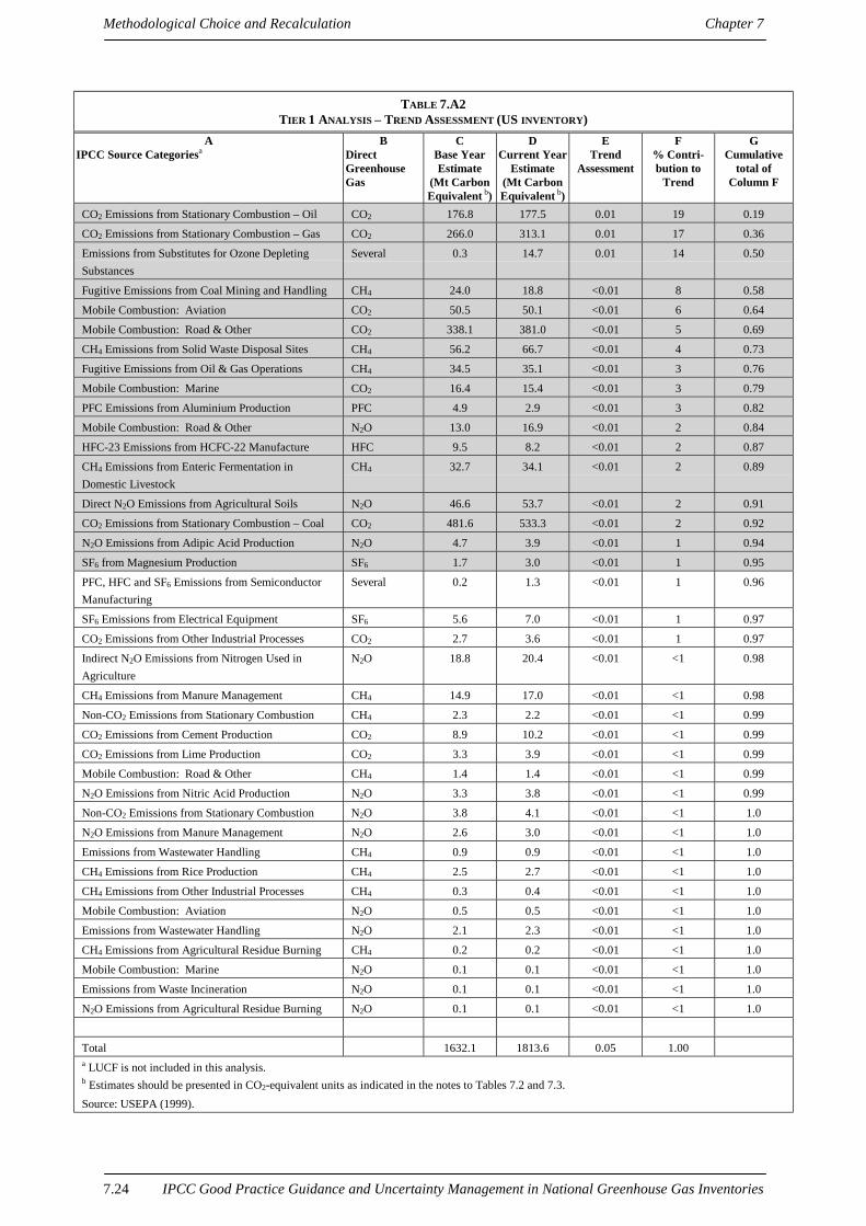
7.24 IPCC Good Practice Guidance and Uncertainty Management in National Greenhouse Gas Inventories
Methodological Choice and Recalculation Chapter 7
TABLE 7.A2TIER 1 ANALYSIS – TREND ASSESSMENT (US INVENTORY)
AIPCC Source Categoriesa
BDirectGreenhouseGas
CBase YearEstimate
(Mt CarbonEquivalent b)
DCurrent Year
Estimate(Mt CarbonEquivalent b)
ETrend
Assessment
F% Contri-bution to
Trend
GCumulative
total ofColumn F
CO2 Emissions from Stationary Combustion – Oil CO2 176.8 177.5 0.01 19 0.19
CO2 Emissions from Stationary Combustion – Gas CO2 266.0 313.1 0.01 17 0.36
Emissions from Substitutes for Ozone DepletingSubstances
Several 0.3 14.7 0.01 14 0.50
Fugitive Emissions from Coal Mining and Handling CH4 24.0 18.8 <0.01 8 0.58
Mobile Combustion: Aviation CO2 50.5 50.1 <0.01 6 0.64
Mobile Combustion: Road & Other CO2 338.1 381.0 <0.01 5 0.69
CH4 Emissions from Solid Waste Disposal Sites CH4 56.2 66.7 <0.01 4 0.73
Fugitive Emissions from Oil & Gas Operations CH4 34.5 35.1 <0.01 3 0.76
Mobile Combustion: Marine CO2 16.4 15.4 <0.01 3 0.79
PFC Emissions from Aluminium Production PFC 4.9 2.9 <0.01 3 0.82
Mobile Combustion: Road & Other N2O 13.0 16.9 <0.01 2 0.84
HFC-23 Emissions from HCFC-22 Manufacture HFC 9.5 8.2 <0.01 2 0.87
CH4 Emissions from Enteric Fermentation inDomestic Livestock
CH4 32.7 34.1 <0.01 2 0.89
Direct N2O Emissions from Agricultural Soils N2O 46.6 53.7 <0.01 2 0.91
CO2 Emissions from Stationary Combustion – Coal CO2 481.6 533.3 <0.01 2 0.92
N2O Emissions from Adipic Acid Production N2O 4.7 3.9 <0.01 1 0.94
SF6 from Magnesium Production SF6 1.7 3.0 <0.01 1 0.95
PFC, HFC and SF6 Emissions from SemiconductorManufacturing
Several 0.2 1.3 <0.01 1 0.96
SF6 Emissions from Electrical Equipment SF6 5.6 7.0 <0.01 1 0.97
CO2 Emissions from Other Industrial Processes CO2 2.7 3.6 <0.01 1 0.97
Indirect N2O Emissions from Nitrogen Used inAgriculture
N2O 18.8 20.4 <0.01 <1 0.98
CH4 Emissions from Manure Management CH4 14.9 17.0 <0.01 <1 0.98
Non-CO2 Emissions from Stationary Combustion CH4 2.3 2.2 <0.01 <1 0.99
CO2 Emissions from Cement Production CO2 8.9 10.2 <0.01 <1 0.99
CO2 Emissions from Lime Production CO2 3.3 3.9 <0.01 <1 0.99
Mobile Combustion: Road & Other CH4 1.4 1.4 <0.01 <1 0.99
N2O Emissions from Nitric Acid Production N2O 3.3 3.8 <0.01 <1 0.99
Non-CO2 Emissions from Stationary Combustion N2O 3.8 4.1 <0.01 <1 1.0
N2O Emissions from Manure Management N2O 2.6 3.0 <0.01 <1 1.0
Emissions from Wastewater Handling CH4 0.9 0.9 <0.01 <1 1.0
CH4 Emissions from Rice Production CH4 2.5 2.7 <0.01 <1 1.0
CH4 Emissions from Other Industrial Processes CH4 0.3 0.4 <0.01 <1 1.0
Mobile Combustion: Aviation N2O 0.5 0.5 <0.01 <1 1.0
Emissions from Wastewater Handling N2O 2.1 2.3 <0.01 <1 1.0
CH4 Emissions from Agricultural Residue Burning CH4 0.2 0.2 <0.01 <1 1.0
Mobile Combustion: Marine N2O 0.1 0.1 <0.01 <1 1.0
Emissions from Waste Incineration N2O 0.1 0.1 <0.01 <1 1.0
N2O Emissions from Agricultural Residue Burning N2O 0.1 0.1 <0.01 <1 1.0
Total 1632.1 1813.6 0.05 1.00a LUCF is not included in this analysis.b Estimates should be presented in CO2-equivalent units as indicated in the notes to Tables 7.2 and 7.3.Source: USEPA (1999).

Chapter 7 Methodological Choice and Recalculation
IPCC Good Practice Guidance and Uncertainty Management in National Greenhouse Gas Inventories 7.25
TABLE 7.A3SOURCE CATEGORY ANALYSIS SUMMARY (US INVENTORY)
Quantitative Method Used : Tier 1 Tier 2A
IPCC Source CategoriesB
DirectGreenhouse Gas
CKey SourceCategory Flag
DIf Column C isYes, Criteria forIdentification
EComments
ENERGY SECTOR
CO2 Emissions from Stationary Combustion – Coal CO2 Yes Level, Trend
CO2 Emissions from Stationary Combustion – Oil CO2 Yes Level, Trend
CO2 Emissions from Stationary Combustion – Gas CO2 Yes Level, Trend
Non-CO2 Emissions from Stationary Combustion CH4 No
Non-CO2 Emissions from Stationary Combustion N2O No
Mobile Combustion: Road & Other CO2 Yes Level, Trend
Mobile Combustion: Road and Other CH4 No
Mobile Combustion: Road and Other N2O Yes Level, Trend
Mobile Combustion: Aviation CO2 Yes Level, Trend
Mobile Combustion: Aviation N2O No
Mobile Combustion: Marine CO2 Yes Trend
Mobile Combustion: Marine N2O No
Fugitive Emissions from Coal Mining and Handling CH4 Yes Level, Trend
Fugitive Emissions from Oil & Gas Operations CH4 Yes Level, Trend
INDUSTRIAL SECTOR
CO2 Emissions from Cement Production CO2 No
CO2 Emissions from Lime Production CO2 No
CO2 Emissions from Other Industrial Processes CO2 No
CH4 Emissions from Other Industrial Processes CH4 No
N2O Emissions from Adipic Acid Production N2O Yes Trend
N2O Emissions from Nitric Acid Production N2O No
PFC Emissions from Aluminium Production PFC Yes Trend
SF6 from Magnesium Production SF6 Yes Trend
SF6 Emissions from Electrical Equipment SF6 No
PFC, HFC and SF6 Emissions from SemiconductorManufacturing
SF6 No
Emissions from Substitutes for Ozone Depleting Substances Several Yes Trend
HFC-23 Emissions from HCFC-22 Manufacture HFC Yes Trend
AGRICULTURE SECTOR
CH4 Emissions from Enteric Fermentation in Domestic Livestock CH4 Yes Level, Trend
CH4 Emissions from Manure Management CH4 Yes Level
N2O Emissions from Manure Management N2O No
Direct N2O Emissions from Agricultural Soils N2O Yes Level, Trend
Indirect N2O Emissions from Nitrogen Used in Agriculture N2O Yes Level
CH4 Emissions from Rice Production CH4 No
CH4 Emissions from Agricultural Residue Burning CH4 No
N2O Emissions from Agricultural Residue Burning N2O No
WASTE SECTOR
CH4 Emissions from Solid Waste Disposal Sites CH4 Yes Level, Trend
Emissions from Wastewater Handling CH4 No
Emissions from Wastewater Handling N2O No
Emissions from Waste Incineration N2O No
✔

7.26 IPCC Good Practice Guidance and Uncertainty Management in National Greenhouse Gas Inventories
Methodological Choice and Recalculation Chapter 7
R E F E R E N C E SFlugsrud, K., W. Irving and K. Rypdal (1999). Methodological Choice in Inventory Preparation. Suggestions for
Good Practice Guidance. Document 1999/19, Statistics Norway.
Intergovernmental Panel on Climate Change (IPCC) (1997). Revised 1996 IPCC Guidelines for NationalGreenhouse Gas Inventories: Volume 3 Reference Manual. J.T. Houghton et al., IPCC/OECD/IEA, Paris,France.
Norwegian Pollution Control Authority (1999). Evaluation of Uncertainty in the Norwegian EmissionsInventory. Norwegian Pollution Control Authority (SFT) Report 99:01, Norway.
USEPA (1999). Inventory of U.S. Greenhouse Gas Emissions and Sinks: 1990-1997. EPA 236-R-99-003, U.S.Environmental Protection Agency.

Chapter 8 Quality Assurance and Quality Control
IPCC Good Practice Guidance and Uncertainty Management in National Greenhouse Gas Inventories 8.1
8
QUALITY ASSURANCE AND QUALITYCONTROL

Quality Assurance and Quality Control Chapter 8
8.2 IPCC Good Practice Guidance and Uncertainty Management in National Greenhouse Gas Inventories
CO-CHAIRS, EDITORS AND EXPERTS
Co-Chairs of the Expert Meeting on Cross-sectoral Methodologies forUncertainty Estimation and Inventory QualityTaka Hiraishi (Japan) and Buruhani Nyenzi (Tanzania)
REVIEW EDITORS
Carlos M Lòpez Cabrera (Cuba) and Leo A Meyer (Netherlands)
Expert Group: Quality Assurance and Quality Control (QA/QC)CO-CHAIRS
Kay Abel (Australia) and Michael Gillenwater (USA)
AUTHOR OF BACKGROUND PAPER
Joe Mangino (USA)
CONTRIBUTORS
Sal Emmanuel (IPCC-NGGIP/TSU), Jean-Pierre Fontelle (France), Michael Gytarsky (Russia), Art Jaques(Canada), Magezi-Akiiki (Uganda), and Joe Mangino (USA)

Chapter 8 Quality Assurance and Quality Control
IPCC Good Practice Guidance and Uncertainty Management in National Greenhouse Gas Inventories 8.3
C o n t e n t s
8 QUALITY ASSURANCE AND QUALITY CONTROL
8.1 INTRODUCTION.................................................................................................................................8.4
8.2 PRACTICAL CONSIDERATIONS IN DEVELOPING QA/QC SYSTEMS......................................8.5
8.3 ELEMENTS OF A QA/QC SYSTEM ..................................................................................................8.6
8.4 INVENTORY AGENCY ......................................................................................................................8.6
8.5 QA/QC PLAN .......................................................................................................................................8.6
8.6 GENERAL QC PROCEDURES (TIER 1)............................................................................................8.7
8.7 SOURCE CATERGORY-SPECIFIC QC PROCEDURES (TIER 2).................................................8.10
8.7.1 Emissions data QC...................................................................................................................8.10
8.7.2 Activity data QC......................................................................................................................8.13
8.7.3 QC of uncertainty estimates.....................................................................................................8.15
8.8 QA PROCEDURES ............................................................................................................................8.15
8.9 VERIFICATION OF EMISSIONS DATA .........................................................................................8.16
8.10 DOCUMENTATION, ARCHIVING AND REPORTING.................................................................8.16
8.10.1 Internal documentation and archiving .....................................................................................8.16
8.10.2 Reporting .................................................................................................................................8.17
REFERENCES ............................................................................................................................................8.17
T a b l e
Table 8.1 Tier 1 General Inventory Level QC Procedures ..............................................................8.8

Quality Assurance and Quality Control Chapter 8
8.4 IPCC Good Practice Guidance and Uncertainty Management in National Greenhouse Gas Inventories
8 QUALITY ASSURANCE ANDQUALITY CONTROL
8 . 1 I N T R O D U C T I O NAn important goal of IPCC good practice guidance is to support the development of national greenhouse gasinventories that can be readily assessed in terms of quality and completeness. It is good practice to implementquality assurance and quality control (QA/QC) procedures in the development of national greenhouse gasinventories to accomplish this goal.
This guidance establishes good practice consistent with the Revised 1996 IPCC Guidelines for NationalGreenhouse Gas Inventories (IPCC Guidelines). The QA/QC good practice guidance outlined here reflectspracticality, acceptability, cost-effectiveness, existing experience, and the potential for application on a world-wide basis. A QA/QC programme contributes to the objectives of good practice guidance, namely to improvetransparency, consistency, comparability, completeness, and confidence in national inventories of emissionsestimates.
The outcomes of the QA/QC process may result in a reassessment of inventory or source category uncertaintyestimates. For example, if data quality is found to be lower than previously thought and this situation cannot berectified in the timeframe of the current inventory, the uncertainty estimates ought to be re-evaluated.
The terms ‘quality control’ and ‘quality assurance’ are often used incorrectly. The definitions of QC and QA inBox 8.1 will be used for the purposes of good practice guidance.
BOX 8.1
DEFINITION OF QA/QC
Quality Control (QC) is a system of routine technical activities, to measure and control the qualityof the inventory as it is being developed. The QC system is designed to:
(i) Provide routine and consistent checks to ensure data integrity, correctness, andcompleteness;
(ii) Identify and address errors and omissions;
(iii) Document and archive inventory material and record all QC activities.
QC activities include general methods such as accuracy checks on data acquisition andcalculations and the use of approved standardised procedures for emission calculations,measurements, estimating uncertainties, archiving information and reporting. Higher tier QCactivities include technical reviews of source categories, activity and emission factor data, andmethods.
Quality Assurance (QA) activities include a planned system of review procedures conducted bypersonnel not directly involved in the inventory compilation/development process. Reviews,preferably by independent third parties, should be performed upon a finalised inventory followingthe implementation of QC procedures. Reviews verify that data quality objectives were met,ensure that the inventory represents the best possible estimates of emissions and sinks given thecurrent state of scientific knowledge and data available, and support the effectiveness of the QCprogramme.
Before implementing QA/QC activities, it is necessary to determine which techniques should be used, and whereand when they will be applied. There are technical and practical considerations in making these decisions. Thetechnical considerations related to the various QA/QC techniques are discussed in general in this chapter, andspecific applications to source categories are described in the source category-specific good practice guidance inChapters 2 to 5. The practical considerations involve assessing national circumstances such as availableresources and expertise and the particular characteristics of the inventory. The level of QA/QC activities shouldbe compatible with the methods or tiers used to estimate emissions for particular source categories. In addition,resources should be focused on priority areas, such as the key source categories (as described in Chapter 7,

Chapter 8 Quality Assurance and Quality Control
IPCC Good Practice Guidance and Uncertainty Management in National Greenhouse Gas Inventories 8.5
Methodological Choice and Recalculation, 7.2, Determining National Key Source Categories) and sourcecategories where changes have occurred in methods or data acquisition since the last inventory compilation.
8 . 2 P R A C T I C A L C O N SI D E R A T I ON S I ND E V E L O P I N G Q A / Q C S Y S T E M S
Implementing QA/QC procedures requires resources, expertise and time. In developing any QA/QC system, it isexpected that judgements will need to be made on the following:
• Resources allocated to QC for different source categories and the compilation process;
• Time allocated to conduct the checks and reviews of emissions estimates;
• Availability and access to information on activity data and emission factors, including data quality;
• Procedures to ensure confidentiality of inventory and source category information, when required;
• Requirements for archiving information;
• Frequency of QA/QC checks on different parts of the inventory;
• The level of QC appropriate for each source category;
• Whether increased effort on QC will result in improved emissions estimates and reduced uncertainties;
• Whether sufficient expertise is available to conduct the checks and reviews.
In practice, the QA/QC system is only part of the inventory development process and inventory agencies do nothave unlimited resources. Quality control requirements, improved accuracy and reduced uncertainty need to bebalanced against requirements for timeliness and cost effectiveness. A good practice system seeks to achievethat balance and to enable continuous improvement of inventory estimates.
Within the QA/QC system, good practice provides for greater effort for key source categories and for thosesource categories where data and methodological changes have recently occurred, than for other sourcecategories. It is unlikely that inventory agencies will have sufficient resources to conduct all the QA/QCprocedures outlined in this chapter on all source categories. In addition, it is not necessary to conduct all of theseprocedures every year. For example, data collection processes conducted by national statistical agencies are notlikely to change significantly from one year to the next. Once the inventory agency has identified what qualitycontrols are in place, assessed the uncertainty of that data, and documented the details for future inventoryreference, it is unnecessary to revisit this aspect of the QC procedure every year. However, it is good practice tocheck the validity of this information periodically as changes in sample size, methods of collection, or frequencyof data collection may occur. The optimal frequency of such checks will depend on national circumstances.
While focusing QA/QC activities on key source categories will lead to the most significant improvements in theoverall inventory estimates, it is good practice to plan to conduct at least the general procedures outlined inSection 8.6, General QC Procedures (Tier 1), on all parts of the inventory over a period of time. Some sourcecategories may require more frequent QA/QC than others because of their significance to the total inventoryestimates, contribution to trends in emissions over time or changes in data or characteristics of the sourcecategory, including the level of uncertainty. For example, if technological advancements occur in an industrialsource category, it is good practice to conduct a thorough QC check of the data sources and the compilationprocess to ensure that the inventory methods remain appropriate.
It is recognised that resource requirements will be higher in the initial stages of implementing any QA/QCsystem than in later years. As capacity to conduct QA/QC procedures develops in the inventory agency and inother associated organisations, improvements in efficiency should be expected.
General QC procedures outlined in Table 8.1, Tier 1 General Inventory Level QC Procedures, and a peer reviewof the inventory estimates are considered minimal QA/QC activities for all inventory compilations. The generalprocedures require no additional expertise in addition to that needed to develop the estimates and compile theinventory and should be performed on estimates developed using Tier 1 or higher tier methods for sourcecategories. A review of the final inventory report by a person not involved in the compilation is also goodpractice, even if the inventory were compiled using only Tier 1 methods. More extensive QC and more rigorousreview processes are encouraged if higher tier methods have been used. Availability of appropriate expertisemay limit the degree of independence of expert reviews in some cases. The QA/QC process is intended to ensuretransparency and quality.
Quality Assurance and Quality Control Chapter 8
8.6 IPCC Good Practice Guidance and Uncertainty Management in National Greenhouse Gas Inventories
There may be some inventory items that involve confidential information, as discussed in Chapters 2 to 5. Theinventory agency should have procedures in place during a review process to ensure that reviewers respect thatconfidentiality.
8 . 3 E L E M E N T S O F A Q A / Q C S Y S T E MThe following are the major elements to be considered in the development of a QA/QC system to beimplemented in tracking inventory compilation:
• An inventory agency responsible for coordinating QA/QC activities;
• A QA/QC plan;
• General QC procedures (Tier 1);
• Source category-specific QC procedures (Tier 2);
• QA review procedures;
• Reporting, documentation, and archiving procedures.
For purposes of the QA/QC system, the Tier 2 QC approach includes all procedures in Tier 1 plus additionalsource category-specific activities.
8 . 4 I N V E N T O R Y A G E N C YThe inventory agency is responsible for coordinating QA/QC activities for the national inventory. The inventoryagency may designate responsibilities for implementing and documenting these QA/QC procedures to otheragencies or organisations. The inventory agency should ensure that other organisations involved in thepreparation of the inventory are following applicable QA/QC procedures.
The inventory agency is also responsible for ensuring that the QA/QC plan is developed and implemented. It isgood practice for the inventory agency to designate a QA/QC coordinator, who would be responsible forensuring that the objectives of the QA/QC programme are implemented.
8 . 5 Q A / Q C P L A NA QA/QC plan is a fundamental element of a QA/QC system, and it is good practice to develop one. The planshould, in general, outline QA/QC activities that will be implemented, and include a scheduled time frame thatfollows inventory preparation from its initial development through to final reporting in any year. It shouldcontain an outline of the processes and schedule to review all source categories.
The QA/QC plan is an internal document to organise, plan, and implement QA/QC activities. Once developed, itcan be referenced and used in subsequent inventory preparation, or modified as appropriate (i.e. when changes inprocesses occur or on advice of independent reviewers). This plan should be available for external review.
In developing and implementing the QA/QC plan, it may be useful to refer to the standards and guidelinespublished by the International Organization for Standardization (ISO), including the ISO 9000 series (see Box8.2). Although ISO 9000 standards are not specifically designed for emissions inventories, they have beenapplied by some countries to help organise QA/QC activities.

Chapter 8 Quality Assurance and Quality Control
IPCC Good Practice Guidance and Uncertainty Management in National Greenhouse Gas Inventories 8.7
BOX 8.2
ISO AS A DATA QUALITY MANAGEMENT SYSTEM
The International Organization for Standardization (ISO) series programme provides standards fordata documentation and audits as part of a quality management system. Though the ISO series isnot designed explicitly for emissions data development, many of the principles may be applied toensure the production of a quality inventory. Inventory agencies may find these documents usefulsource material for developing QA/QC plans for greenhouse gas inventories. Some countries (e.g.the United Kingdom and the Netherlands) have already applied some elements of the ISOstandards for their inventory development process and data management.
The following standards and guidelines published under the ISO series may supplement sourcecategory-specific QA/QC procedures for inventory development and provide practical guidancefor ensuring data quality and a transparent reporting system.
ISO 9004-1: General quality guidelines to implement a quality system.
ISO 9004-4: Guidelines for implementing continuous quality improvement within theorganisation, using tools and techniques based on data collection and analysis.
ISO 10005: Guidance on how to prepare quality plans for the control of specific projects.
ISO 10011-1: Guidelines for auditing a quality system.
ISO 10011-2: Guidance on the qualification criteria for quality systems auditors.
ISO 10011-3: Guidelines for managing quality system audit programmes.
ISO 10012: Guidelines on calibration systems and statistical controls to ensure thatmeasurements are made with the intended accuracy.
ISO 10013: Guidelines for developing quality manuals to meet specific needs.
Source: http://www.iso.ch/
8 . 6 G E N E R A L Q C P R O C E D U R E S ( T I E R 1 )The focus of general QC techniques is on the processing, handling, documenting, archiving and reportingprocedures that are common to all the inventory source categories. Table 8.1, Tier 1 General Inventory Level QCProcedures, lists the general QC checks that the inventory agency should use routinely throughout thepreparation of the annual inventory. Most of the checks shown in Table 8.1 could be performed by cross-checks,recalculation, or through visual inspections. The results of these QC activities and procedures should bedocumented as set out in Section 8.10.1, Internal Documentation and Archiving, below. If checks are performedelectronically, these systems should be periodically reviewed to ensure the integrity of the checking function.
It will not be possible to check all aspects of inventory input data, parameters and calculations every year.Checks may be performed on selected sets of data and processes, such that identified key source categories areconsidered every year. Checks on other source categories may be conducted less frequently. However, a sampleof data and calculations from every sector should be included in the QC process each year to ensure that allsectors are addressed on an ongoing basis. In establishing criteria and processes for selecting the sample data setsand processes, it is good practice for the inventory agency to plan to undertake QC checks on all parts of theinventory over an appropriate period of time.

Quality Assurance and Quality Control Chapter 8
8.8 IPCC Good Practice Guidance and Uncertainty Management in National Greenhouse Gas Inventories
TABLE 8.1
TIER 1 GENERAL INVENTORY LEVEL QC PROCEDURES
QC Activity Procedures
Check that assumptions and criteria for the selection ofactivity data and emission factors are documented.
• Cross-check descriptions of activity data and emissionfactors with information on source categories and ensurethat these are properly recorded and archived.
Check for transcription errors in data input and reference
• Confirm that bibliographical data references are properlycited in the internal documentation.
• Cross-check a sample of input data from each sourcecategory (either measurements or parameters used incalculations) for transcription errors.
Check that emissions are calculated correctly.
• Reproduce a representative sample of emissionscalculations.
• Selectively mimic complex model calculations withabbreviated calculations to judge relative accuracy.
Check that parameter and emission units arecorrectly recorded and that appropriate conversionfactors are used.
• Check that units are properly labelled in calculation sheets.
• Check that units are correctly carried through frombeginning to end of calculations.
• Check that conversion factors are correct.
• Check that temporal and spatial adjustment factors are usedcorrectly.
Check the integrity of database files.
• Confirm that the appropriate data processing steps arecorrectly represented in the database.
• Confirm that data relationships are correctly represented inthe database.
• Ensure that data fields are properly labelled and have thecorrect design specifications.
• Ensure that adequate documentation of database and modelstructure and operation are archived.
Check for consistency in data between sourcecategories.
• Identify parameters (e.g. activity data, constants) that arecommon to multiple source categories and confirm that thereis consistency in the values used for these parameters in theemissions calculations.
Check that the movement of inventory data amongprocessing steps is correct.
• Check that emissions data are correctly aggregated fromlower reporting levels to higher reporting levels whenpreparing summaries.
• Check that emissions data are correctly transcribed betweendifferent intermediate products.

Chapter 8 Quality Assurance and Quality Control
IPCC Good Practice Guidance and Uncertainty Management in National Greenhouse Gas Inventories 8.9
TABLE 8.1 (CONTINUED)
TIER 1 GENERAL INVENTORY LEVEL QC PROCEDURES
QC Activity Procedures
Check that uncertainties in emissions and removals areestimated or calculated correctly.
• Check that qualifications of individuals providing expertjudgement for uncertainty estimates are appropriate.
• Check that qualifications, assumptions and expertjudgements are recorded. Check that calculateduncertainties are complete and calculated correctly.
• If necessary, duplicate error calculations or a small sampleof the probability distributions used by Monte Carloanalyses.
Undertake review of internal documentation.
• Check that there is detailed internal documentation tosupport the estimates and enable duplication of the emissionand uncertainty estimates.
• Check that inventory data, supporting data, and inventoryrecords are archived and stored to facilitate detailed review.
• Check integrity of any data archiving arrangements ofoutside organisations involved in inventory preparation.
Check methodological and data changes resulting in re-calculations.
• Check for temporal consistency in time series input data foreach source category.
• Check for consistency in the algorithm/method used forcalculations throughout the time series.
Undertake completeness checks.
• Confirm that estimates are reported for all source categoriesand for all years from the appropriate base year to theperiod of the current inventory.
• Check that known data gaps that result in incomplete sourcecategory emissions estimates are documented.
Compare estimates to previous estimates.
• For each source category, current inventory estimatesshould be compared to previous estimates. If there aresignificant changes or departures from expected trends, re-check estimates and explain any difference.
The checks in Table 8.1, should be applied irrespective of the type of data used to develop the inventoryestimates and are equally applicable to source categories where default values or national data are used as thebasis for the estimates.
In some cases, emissions estimates are prepared for the inventory agency by outside consultants or agencies. Theinventory agency should ensure that the QC checks listed in Table 8.1, Tier 1 General Inventory Level QCProcedure, are communicated to the consultants/agencies. This will assist in making sure that QC procedures areperformed and recorded by the consultant or outside agency. The inventory agency should review these QA/QCactivities. In cases where official national statistics are relied upon – primarily for activity data – QC proceduresmay already have been implemented on these national data. However, it is good practice for the inventoryagency to confirm that national statistical agencies have implemented adequate QC procedures equivalent tothose in Table 8.1.
Due to the quantity of data that needs to be checked for some source categories, automated checks areencouraged where possible. For example, one of the most common QC activities involves checking that datakeyed into a computer database are correct. A QC procedure could be set up to use an automated range check(based on the range of expected values of the input data from the original reference) for the input values asrecorded in the database. A combination of manual and automated checks may constitute the most effectiveprocedures in checking large quantities of input data.

Quality Assurance and Quality Control Chapter 8
8.10 IPCC Good Practice Guidance and Uncertainty Management in National Greenhouse Gas Inventories
8 . 7 S O U R C E C A T E R G O R Y - S P E C I FI C Q CP R O C E D U R E S ( T IE R 2 )
In contrast to general inventory QC techniques, source category-specific QC procedures are directed at specifictypes of data used in the methods for individual source categories and require knowledge of the emission sourcecategory, the types of data available and the parameters associated with emissions.
It is important to note that Tier 2 source category-specific QC activities are in addition to the general QCconducted as part of Tier 1 (i.e. include QC checks listed in Table 8.1). The source category-specific measuresare applied on a case-by-case basis focusing on key source categories (see Chapter 7, Methodological Choiceand Recalculation) and on source categories where significant methodological and data revisions have takenplace. It is good practice that inventory agencies applying higher tier methods in compiling national inventoriesutilise Tier 2 QC procedures. Specific applications of source category-specific Tier 2 QC procedures areprovided in the energy, agriculture, industrial processes and waste chapters of this report (Chapters 2 to 5).
Source category-specific QC activities include the following:
• Emission data QC;
• Activity data QC;
• QC of uncertainty estimates.
The first two activities relate to the types of data used to prepare the emissions estimates for a given sourcecategory. QC of uncertainty estimates covers activities associated with determining uncertainties in emissionsestimates (for more information on the determination of these uncertainties, see Chapter 6, QuantifyingUncertainties in Practice).
The actual QC procedures that need to be implemented by the inventory agency will depend on the method usedto estimate the emissions for a given source category. If estimates are developed by outside agencies, theinventory agency may, upon review, reference the QC activities of the outside agency as part of the QA/QC plan.There is no need to duplicate QC activities if the inventory agency is satisfied that the QC activities performedby the outside agency meet the minimum requirements of the QA/QC plan.
8 . 7 . 1 E mi s s i o n s d a t a QCThe following sections describe QC checks on IPCC default factors, country-specific emission factors, and directemission measurements from individual sites (used either as the basis for a site-specific emission factor ordirectly for an emissions estimate). Emission comparison procedures are described in Section 8.7.1.4, EmissionComparisons. Inventory agencies should take into account the practical considerations discussed in Section 8.2,Practical Considerations in Developing QA/QC Systems, when determining what level of QC activities toundertake.
8.7.1.1 IPCC DEFAULT EMISSION FACTORSWhere IPCC default emission factors are used, it is good practice for the inventory agency to assess theapplicability of these factors to national circumstances. This assessment may include an evaluation of nationalconditions compared to the context of the studies upon which the IPCC default factors were based. If there isinsufficient information on the context of the IPCC default factors, the inventory agency should take account ofthis in assessing the uncertainty of the national emissions estimates based on the IPCC default emission factors.For key source categories, inventory agencies should consider options for obtaining emission factors that areknown to be representative of national circumstances. The results of this assessment should be documented.
If possible, IPCC default emission factor checks could be supplemented by comparisons with national site orplant-level factors to determine their representativeness relative to actual sources in the country. Thissupplementary check is good practice even if data are only available for a small percentage of sites or plants.
8.7.1.2 COUNTRY-SPECIFIC EMISSION FACTORSCountry-specific emission factors may be developed at a national or other aggregated level within the countrybased on prevailing technology, science, local characteristics and other criteria. These factors are not necessarily

Chapter 8 Quality Assurance and Quality Control
IPCC Good Practice Guidance and Uncertainty Management in National Greenhouse Gas Inventories 8.11
site-specific, but are used to represent a source category or sub-source category. Two steps are necessary toensure good practice emission factor QC for country-specific factors.
The first is to perform QC checks on the data used to develop the emission factors. The adequacy of the emissionfactors and the QA/QC performed during their development should be assessed. If emission factors weredeveloped based on site-specific or source-level testing, then the inventory agency should check if themeasurement programme included appropriate QC procedures.
Frequently, country-specific emission factors will be based on secondary data sources, such as published studiesor other literature.1 In these cases, the inventory agency could attempt to determine whether the QC activitiesconducted during the original preparation of the data are consistent with the applicable QC procedures outlinedin Table 8.1 and whether any limitations of the secondary data have been identified and documented. Theinventory agency could also attempt to establish whether the secondary data have undergone peer review andrecord the scope of such a review.
If it is determined that the QA/QC associated with the secondary data is adequate, then the inventory agency cansimply reference the data source for QC documentation and document the applicability of the data for use inemissions estimates.
If it is determined that the QA/QC associated with the secondary data is inadequate, then the inventory agencyshould attempt to have QA/QC checks on the secondary data established. It should also reassess the uncertaintyof any emissions estimates derived from the secondary data. The inventory agency may also reconsider how thedata are used and whether any alternative data, (including IPCC default values) may provide a better estimate ofemissions from this source category.
Second, country-specific factors and circumstances should be compared with relevant IPCC default factors andthe characteristics of the studies on which the default factors are based. The intent of this comparison is todetermine whether country-specific factors are reasonable, given similarities or differences between the nationalsource category and the ‘average’ source category represented by the defaults. Large differences betweencountry-specific factors and default factors should be explained and documented.
A supplementary step is to compare the country-specific factors with site-specific or plant-level factors if theseare available. For example, if there are emission factors available for a few plants (but not enough to support abottom-up approach) these plant-specific factors could be compared with the aggregated factor used in theinventory. This type of comparison provides an indication of both the reasonableness of the country-specificfactor and its representativeness.
8.7.1.3 DIRECT EMISSION MEASUREMENTSEmissions from a source category may be estimated using direct measurements in the following ways:
• Sample emissions measurements from a facility may be used to develop a representative emission factor forthat individual site, or for the entire category (i.e. for development of a national level emission factor);
• Continuous emissions monitoring (CEM) data may be used to compile an annual estimate of emissions for aparticular process. In theory, CEM can provide a complete set of quantified emissions data across theinventory period for an individual facility process, and does not have to be correlated back to a processparameter or input variable like an emission factor.
Regardless of how direct measurement data are being used, the inventory agency should review the processesand check the measurements as part of the QC activities.
Use of standard measurement methods improves the consistency of resulting data and knowledge of thestatistical properties of the data. If standard reference methods for measuring specific greenhouse gas emissions(and removals) are available, inventory agencies should encourage plants to use these. If specific standardmethods are not available, the inventory agency should confirm whether nationally or internationally recognisedstandard methods such as ISO 10012 are used for measurements and whether the measurement equipment iscalibrated and maintained properly.
For example, ISO has published standards that specify procedures to quantify some of the performancecharacteristics of all air quality measurement methods such as bias, calibration, instability, lower detectionlimits, sensitivity, and upper limits of measurement (ISO, 1994). While these standards are not associated with a
1 Secondary data sources refer to reference sources for inventory data that are not designed for the express purpose ofinventory development. Secondary data sources typically include national statistical databases, scientific literature, and otherstudies produced by agencies or organisations not associated with the inventory development.

Quality Assurance and Quality Control Chapter 8
8.12 IPCC Good Practice Guidance and Uncertainty Management in National Greenhouse Gas Inventories
reference method for a specific greenhouse gas source category, they have direct application to QC activitiesassociated with estimations based on measured emission values.
Where direct measurement data from individual sites are in question, discussions with site managers can beuseful to encourage improvement of the QA/QC practices at the sites. Also, supplementary QC activities areencouraged for bottom-up methods based on site-specific emission factors where significant uncertainty remainsin the estimates. Site-specific factors can be compared between sites and also to IPCC or national level defaults.Significant differences between sites or between a particular site and the IPCC defaults should elicit furtherreview and checks on calculations. Large differences should be explained and documented.
8.7.1.4 EMISSION COMPARISONSIt is standard QC practice to compare emissions from each source category with emissions previously providedfrom the same source category or against historical trends and reference calculations as described below. Theobjective of these comparisons (often referred to as ‘reality checks’) is to ensure that the emission values are notwildly improbable or that they fall within a range that is considered reasonable. If the estimates seemunreasonable, emission checks can lead to a re-evaluation of emission factors and activity data before theinventory process has advanced to its final stages.
The first step of an emissions comparison is a consistency and completeness check using available historicalinventory data for multiple years. The emission levels of most source categories do not abruptly change fromyear to year, as changes in both activity data and emission factors are generally gradual. In most circumstances,the change in emissions will be less than 10% per year. Thus, significant changes in emissions from previousyears may indicate possible input or calculation errors. After calculating differences, the larger percentagedifferences (in any direction) should be flagged, by visual inspection of the list, by visual inspection of thegraphical presentation of differences (e.g. in a spreadsheet) or by using a dedicated software programme thatputs flags and rankings in the list of differences.
It is good practice to also check the annual increase or decrease of changes in emissions levels in significant sub-source categories of some source categories. Sub-source categories may show greater percentage changes thanthe aggregated source categories. For example, total emissions from petrol cars are not likely to changesubstantially on an annual basis, but emissions from sub-source categories, such as catalyst-equipped petrol cars,may show substantial changes if the market share is not in equilibrium or if the technology is changing andrapidly being adopted in the marketplace.
It is good practice to check the emissions estimates for all source categories or sub-source categories that showgreater than 10% change in a year compared to the previous year’s inventory. Source categories and sub-sourcecategories should be ranked according to the percentage difference in emissions from the previous year.
Supplementary emission comparisons can also be performed, if appropriate, including order-of-magnitudechecks and reference calculations.
ORDER-OF-MAGNITUDE CHECKSOrder of magnitude checks look for major calculation errors and exclusion of major source categories or sub-source categories. Method-based comparisons may be made depending on whether the emissions for the sourcecategory were determined using a top-down or bottom-up approach. For example, if N2O estimates for nitric acidproduction were determined using a bottom-up approach (i.e. emissions estimates were determined for eachindividual production plant based on plant-specific data), the emissions check would consist of comparing thesum of the individual plant-level emissions to a top-down emission estimate based on national nitric acidproduction figures and IPCC default Tier 1 factors. If significant differences are found in the comparison, furtherinvestigation using the source category-specific QC techniques described in Section 8.7, Source Category-Specific QC Procedures (Tier 2), would be necessary to answer the following questions:
• Are there inaccuracies associated with any of the individual plant estimates (e.g. an extreme outlier may beaccounting for an unreasonable quantity of emissions)?
• Are the plant-specific emission factors significantly different from each other?
• Are the plant-specific production rates consistent with published national level production rates?
• Is there any other explanation for a significant difference, such as the effect of controls, the manner in whichproduction is reported or possibly undocumented assumptions?
This is an example of how the result of a relatively simple emission check can lead to a more intensiveinvestigation of the representativeness of the emissions data. Knowledge of the source category is required to

Chapter 8 Quality Assurance and Quality Control
IPCC Good Practice Guidance and Uncertainty Management in National Greenhouse Gas Inventories 8.13
isolate the parameter that is causing the difference in emissions estimates and to understand the reasons for thedifference.
REFERENCE CALCULATIONSAnother emission comparison may be used for source categories that rely on empirical formulas for thecalculation of emissions. Where such formulas are used, final calculated emission levels should followstochiometric ratios and conserve energy and mass. In a number of cases where emissions are calculated as thesum of sectoral activities based on the consumption of a specific commodity (e.g. fuels or products like HFCs,PFCs or SF6), the emissions could alternatively be estimated using apparent consumption figures: national totalproduction + import – export ± stock changes. For CO2 from fossil fuel combustion, a reference calculationbased on apparent fuel consumption per fuel type is mandatory according to the IPCC Guidelines. Anotherexample is estimating emissions from manure management. The total quantity of methane produced should notexceed the quantity that could be expected based on the carbon content of the volatile solids in the manure.
Discrepancies between inventory data and reference calculations do not necessarily imply that the inventory dataare in error. It is important to consider that there may be large uncertainties associated with the referencecalculations themselves when analysing discrepancies.
8 . 7 . 2 A c t i v i ty da t a Q CThe estimation methods for many source categories rely on the use of activity data and associated input variablesthat are not directly prepared by the inventory agency. Activity data is normally collated at a national level usingsecondary data sources or from site-specific data prepared by site or plant personnel from their ownmeasurements. Inventory agencies should take into account the practical considerations discussed above whendetermining the level of QC activities to undertake.
8.7.2.1 NATIONAL LEVEL ACTIVITY DATAWhere national activity data from secondary data sources are used in the inventory, it is good practice for theinventory agency or its designees to evaluate and document the associated QA/QC activities. This is particularlyimportant with regard to activity data, since most activity data are originally prepared for purposes other than asinput to estimates of greenhouse gas emissions. Though not always readily available, many statisticalorganisations, for example, have their own procedures for assessing the quality of the data independently of whatthe end use of the data may be. If it is determined that these procedures satisfy minimum activities listed in theQA/QC plan, the inventory agency can simply reference the QA/QC activities conducted by the statisticalorganisation.
It is good practice for the inventory agency to determine if the level of QC associated with secondary activitydata includes those QC procedures listed in Table 8.1. In addition, the inventory agency may establish whetherthe secondary data have been peer reviewed and record the scope of this review. If it is determined that theQA/QC associated with the secondary data is adequate, then the inventory agency can simply reference the datasource and document the applicability of the data for use in its emissions estimates.
If it is determined that the QC associated with the secondary data is inadequate, then the inventory agency shouldattempt to have QA/QC checks on the secondary data established. It should also reassess the uncertainty ofemissions estimates in light of the findings from its assessment of the QA/QC associated with secondary data.The inventory agency should also reconsider how the data are used and whether any alternative data, includingIPCC default values and international data sets, may provide for a better estimate of emissions. If no alternativedata sources are available, the inventory agency should document the inadequacies associated with the secondarydata QC as part of its summary report on QA/QC (see Section 8.10.2, Reporting, for reporting guidance).
For example, in the transportation category, countries typically use either fuel usage or kilometer (km) statisticsto develop emissions estimates. The national statistics on fuel usage and kms travelled by vehicles are usuallyprepared by a different agency from the inventory agency. However, it is the responsibility of the inventoryagency to determine what QA/QC activities were implemented by the agency that prepared the original fuelusage and km statistics for vehicles. Questions that may be asked in this context are:
• Does the statistical agency have a QA/QC plan that covers the preparation of the data?
• What sampling protocol was used to estimate fuel usage or kms travelled?
• How recently was the sampling protocol reviewed?
• Has any potential bias in the data been identified by the statistical agency?

Quality Assurance and Quality Control Chapter 8
8.14 IPCC Good Practice Guidance and Uncertainty Management in National Greenhouse Gas Inventories
• Has the statistical agency identified and documented uncertainties in the data?
• Has the statistical agency identified and documented errors in the data?
National level activity data should be compared with previous year’s data for the source category beingevaluated. Activity data for most source categories tend to exhibit relatively consistent changes from year to yearwithout sharp increases or decreases. If the national activity data for any year diverge greatly from the historicaltrend, the activity data should be checked for errors. If the general mathematical checks do not reveal errors, thecharacteristics of the source category could be investigated and any change identified and documented.
Where possible, a comparison check of activity data from multiple reference sources should be undertaken. Thisis important for source categories that have a high level of uncertainty associated with their estimates. Forexample, many of the agricultural source-categories rely on government statistics for activity data such aslivestock populations, areas under cultivation, and the extent of prescribed burning. Similar statistics may beprepared by industry, universities, or other organisations and can be used to compare with standard referencesources. As part of the QC check, the inventory agency should ascertain whether independent data have beenused to derive alternative activity data sets. In some cases, the same data are treated differently by differentagencies to meet varying needs. Comparisons may need to be made at a regional level or with a subset of thenational data since many alternative references for such activity data have limited scope and do not cover theentire nation.
8.7.2.2 SITE-SPECIFIC ACTIVITY DATASome methods rely on the use of site-specific activity data used in conjunction with IPCC default or country-specific emission factors. Site or plant personnel typically prepare these estimates of activity, often for purposesother than as inputs to emissions inventories. QC checks should focus on inconsistencies between sites toestablish whether these reflect errors, different measurement techniques, or real differences in emissions,operating conditions or technology.
A variety of QC checks can be used to identify errors in site-level activity data. The inventory agency shouldestablish whether recognised national or international standards were used in measuring activity data at theindividual sites. If measurements were made according to recognised national or international standards and aQA/QC process is in place, the inventory agency should satisfy itself that the QA/QC process at the site isacceptable under the inventory QA/QC plan and at least includes Tier 1 activities. Acceptable QC procedures inuse at the site may be directly referenced. If the measurements were not made using standard methods andQA/QC is not of an acceptable standard, then the use of these activity data should be carefully evaluated,uncertainty estimates reconsidered, and qualifications documented.
Comparisons of activity data from different reference sources may also be used to expand the activity data QC.For example, in estimating PFC emissions from primary aluminium smelting, many inventory agencies usesmelter-specific activity data to prepare the inventory estimates. A QC check of the aggregated activity data fromall aluminium smelters can be made against national production statistics for the industry. Also, production datacan be compared across different sites, possibly with adjustments made for plant capacities, to evaluate thereasonableness of the production data. Similar comparisons of activity data can be made for othermanufacturing-based source categories where there are published data on national production. If outliers areidentified, they should be investigated to determine if the difference can be explained by the uniquecharacteristics of the site or there is an error in the reported activity.
Site-specific activity data checks may also be applied to methods based on product usage. For example, onemethod for estimating SF6 emissions from use in electrical equipment relies on an account balance of gaspurchases, gas sales for recycling, the amount of gas stored on site (outside of equipment), handling losses,refills for maintenance, and the total holding capacity of the equipment system. This account balance systemshould be used at each facility where the equipment is in place. A QC check of overall national activity could bemade by performing the same kind of account balancing procedure on a national basis. This national accountbalancing would consider national sales of SF6 for use in electrical equipment, the nation-wide increase in thetotal handling capacity of the equipment (that may be obtained from equipment manufacturers), and the quantityof SF6 destroyed in the country. The results of the bottom-up and top-down account balancing analyses shouldagree or large differences should be explained. Similar accounting techniques can be used as QC checks on othercategories based on gas usage (e.g. substitutes for ozone-depleting substances) to check consumption andemissions.

Chapter 8 Quality Assurance and Quality Control
IPCC Good Practice Guidance and Uncertainty Management in National Greenhouse Gas Inventories 8.15
8 . 7 . 3 Q C o f u n c e r t a i n ty e s t i ma t e sQC should also be undertaken on calculations or estimates of uncertainty associated with emissions estimates.Good practice for estimating inventory uncertainties is described in Chapter 6, Quantifying Uncertainties inPractice, and relies on calculations of uncertainty at the source category level that are then combined to summarylevels for the entire inventory. Some of the methods rely on the use of measured data associated with theemission factors or activity data to develop probability density functions from which uncertainty estimates canbe made. In the absence of measured data, many uncertainty estimates will rely on expert judgement.
It is good practice for QC procedures to be applied to the uncertainty estimations to confirm that calculations arecorrect and that there is sufficient documentation to duplicate them. The assumptions on which uncertaintyestimations have been based should be documented for each source category. Calculations of source category-specific and aggregated uncertainty estimates should be checked and any errors addressed. For uncertaintyestimates involving expert judgement, the qualifications of experts should also be checked and documented, asshould the process of eliciting expert judgement, including information on the data considered, literaturereferences, assumptions made and scenarios considered. Chapter 6 contains advice on how to document expertjudgements on uncertainties.
8 . 8 Q A P R O C E D U R E SGood practice for QA procedures requires an objective review to assess the quality of the inventory, and also toidentify areas where improvements could be made. The inventory may be reviewed as a whole or in parts. QAprocedures are utilised in addition to the Tier 1 and Tier 2 QC. The objective in QA implementation is to involvereviewers that can conduct an unbiased review of the inventory. It is good practice to use QA reviewers thathave not been involved in preparing the inventory. Preferably these reviewers would be independent expertsfrom other agencies or a national or international expert or group not closely connected with national inventorycompilation. Where third party reviewers outside the inventory agency are not available, staff from another partof the inventory agency not involved in the portion of the inventory being reviewed can also fulfil QA roles.
It is good practice for inventory agencies to conduct a basic expert peer review (Tier 1 QA) prior to inventorysubmission in order to identify potential problems and make corrections where possible. It is also good practiceto apply this review to all source categories in the inventory. However, this will not always be practical due totiming and resource constraints. Key source categories should be given priority as well as source categorieswhere significant changes in methods or data have been made. Inventory agencies may also choose to performmore extensive peer reviews or audits or both as additional (Tier 2) QA procedures within the availableresources.
More specific information on QA procedures related to individual source categories is provided in the sourcecategory-specific QA/QC sections in Chapters 2 to 5.
EXPERT PEER REVIEWExpert peer review consists of a review of calculations or assumptions by experts in relevant technical fields.This procedure is generally accomplished by reviewing the documentation associated with the methods andresults, but usually does not include rigorous certification of data or references such as might be undertaken in anaudit. The objective of the expert peer review is to ensure that the inventory’s results, assumptions, and methodsare reasonable as judged by those knowledgeable in the specific field. Expert review processes may involvetechnical experts and, where a country has formal stakeholder and public review mechanisms in place, thesereviews can supplement but not replace expert peer review.
There are no standard tools or mechanisms for expert peer review, and its use should be considered on a case-by-case basis. If there is a high level of uncertainty associated with an emission estimate for a source category,expert peer review may provide information to improve the estimate, or at least to better quantify the uncertainty.Expert reviews may be conducted on all parts of a source category. For example, if the activity data estimatesfrom oil and natural gas production are to be reviewed but not the emission factors, experts in the oil and gasindustry could be involved in the review to provide industry expertise even if they do not have direct experiencein greenhouse gas emissions estimation. Effective peer reviews often involve identifying and contacting keyindustrial trade organisations associated with specific source categories. It is preferable for this expert input to besought early in the inventory development process so that the experts can participate from the start. It is goodpractice to involve relevant experts in development and review of methods and data acquisition.

Quality Assurance and Quality Control Chapter 8
8.16 IPCC Good Practice Guidance and Uncertainty Management in National Greenhouse Gas Inventories
The results of expert peer review, and the response of the inventory agency to those findings, may be importantto widespread acceptance of the final inventory. All expert peer reviews should be well documented, preferablyin a report or checklist format that shows the findings and recommendations for improvement.
AUDITSFor the purpose of good practice in inventory preparation, audits may be used to evaluate how effectively theinventory agency complies with the minimum QC specifications outlined in the QC plan. It is important that theauditor be independent of the inventory agency as much as possible so as to be able to provide an objectiveassessment of the processes and data evaluated. Audits may be conducted during the preparation of an inventory,following inventory preparation, or on a previous inventory. Audits are especially useful when new emissionestimation methods are adopted, or when there are substantial changes to existing methods. It is desirable for theinventory agency to develop a schedule of audits at strategic points in the inventory development. For example,audits related to initial data collection, measurement work, transcription, calculation and documentation may beconducted. Audits can be used to verify that the QC steps identified in Table 8.1 have been implemented and thatsource category-specific QC procedures have been implemented according to the QC plan.
8 . 9 V E R I F I C AT I O N O F E M I S S I O N S D AT AOptions for inventory verification processes are described in Annex 2, Verification. Verification techniques canbe applied during inventory development as well as after the inventory is compiled.
Comparisons with other independently compiled, national emissions data (if available) are a quick option toevaluate completeness, approximate emission levels and correct source category allocations. These comparisonscan be made for different greenhouse gases at national, sectoral, source category, and sub-source category levels,as far as the differences in definitions enable them.
Although the inventory agency is ultimately responsible for the compilation and submission of the nationalgreenhouse gas inventory, other independent publications on this subject may be available (e.g. from scientificliterature or other institutes or agencies). These documents may provide the means for comparisons with othernational estimates.
The verification process can help evaluate the uncertainty in emissions estimates, taking into account the qualityand context of both the original inventory data and data used for verification purposes. Where verificationtechniques are used, they should be reflected in the QA/QC plan. Improvements resulting from verificationshould be documented, as should detailed results of the verification process.
8 . 1 0 D O C U M E N T A T I O N , A R C H I V I N G A N DR E P O R T I N G
8 . 1 0 . 1 I n t e r na l do c u me n t a t i o n a n d a r c h i v i n gAs part of general QC procedures, it is good practice to document and archive all information required toproduce the national emissions inventory estimates. This includes:
• Assumptions and criteria for selection of activity data and emission factors;
• Emission factors used, including references to the IPCC document for default factors or to publishedreferences or other documentation for emission factors used in higher tier methods;
• Activity data or sufficient information to enable activity data to be traced to the referenced source;
• Information on the uncertainty associated with activity data and emission factors;
• Rationale for choice of methods;
• Methods used, including those used to estimate uncertainty;
• Changes in data inputs or methods from previous years;
• Identification of individuals providing expert judgement for uncertainty estimates and their qualifications todo so;

Chapter 8 Quality Assurance and Quality Control
IPCC Good Practice Guidance and Uncertainty Management in National Greenhouse Gas Inventories 8.17
• Details of electronic databases or software used in production of the inventory, including versions, operatingmanuals, hardware requirements and any other information required to enable their later use;
• Worksheets and interim calculations for source category estimates and aggregated estimates and any re-calculations of previous estimates;
• Final inventory report and any analysis of trends from previous years;
• QA/QC plans and outcomes of QA/QC procedures.
It is good practice for inventory agencies to maintain this documentation for every annual inventory producedand to provide it for review. It is good practice to maintain and archive this documentation in such a way thatevery inventory estimate can be fully documented and reproduced if necessary. Inventory agencies should ensurethat records are unambiguous; for example, a reference to ‘IPCC default factor’ is not sufficient. A full referenceto the particular document (e.g. Revised 1996 IPCC Guidelines for National Greenhouse Gas Inventories) isnecessary in order to identify the source of the emission factor because there may have been several updates ofdefault factors as new information has become available.
Records of QA/QC procedures are important information to enable continuous improvement to inventoryestimates. It is good practice for records of QA/QC activities to include the checks/audits/reviews that wereperformed, when they were performed, who performed them, and corrections and modifications to the inventoryresulting from the QA/QC activity.
8 . 1 0 . 2 R e p o r t in gIt is good practice to report a summary of implemented QA/QC activities and key findings as a supplement toeach country’s national inventory. However, it is not practical or necessary to report all the internaldocumentation that is retained by the inventory agency. The summary should describe which activities wereperformed internally and what external reviews were conducted for each source category and on the entireinventory in accordance with the QA/QC plan. The key findings should describe major issues regarding qualityof input data, methods, processing, or archiving and show how they were addressed or plan to be addressed inthe future.
R E F E R E N CE SIntergovernmental Panel on Climate Change (IPCC) (1997). Revised 1996 IPCC Guidelines for National
Greenhouse Gas Inventoires: Volumes 1, 2 and 3. J.T. Houghton et al., IPCC/OECD/IEA, Paris, France.
International Organization for Standardization (ISO) (1994). Air Quality, Determination of PerformanceCharacteristics of Measurement Methods. ISO 9196:1994. ISO, Geneva, Switzerland.

Annex 1 Conceptual Basis for Uncertainty Analysis
IPCC Good Practice Guidance and Uncertainty Management in National Greenhouse Gas Inventories A1.1
A N N E X 1
CONCEPTUAL BASIS FORUNCERTAINTY ANALYSIS

Conceptual Basis for Uncertainty Analysis Annex 1
IPCC Good Practice Guidance and Uncertainty Management in National Greenhouse Gas InventoriesA1.2
CO-CHAIRS, EDITORS AND EXPERTS
Co-chairs of the Expert Meeting on Cross-sectoral Methodologies forUncertainty Estimation and Inventory QualityTaka Hiraishi (Japan) and Buruhani Nyenzi (Tanzania)
REVIEW EDITOR
Richard Odingo (Kenya)
Expert Group: Conceptual Basis for Uncertainty AnalysisCO-CHAIRS
Ian Galbally (Australia) and Newton Paciornik (Brazil)
AUTHORS OF BACKGROUND PAPERS
Ian Galbally (Australia), Newton Paciornik (Brazil), and Milos Tichy (Czech Republic)
CONTRIBUTORS
Wiley Barbour (USA), Leandro Buendia (IPCC-NGGIP/TSU), Franck Jacobs (Antigua), Naoki Matsuo (Japan),Richard Odingo (Kenya), Daniela Romano (Italy), and Milos Tichy (Czech Republic)

Annex 1 Conceptual Basis for Uncertainty Analysis
IPCC Good Practice Guidance and Uncertainty Management in National Greenhouse Gas Inventories A1.3
C o n t e n t s
ANNEX 1 CONCEPTUAL BASIS FOR UNCERTAINTY ANALYSIS
A1.1 INTRODUCTION........................................................................................................................... A1.5
A1.2 STATISTICAL CONCEPTS .......................................................................................................... A1.5
A1.2.1 Expressing uncertainty............................................................................................................ A1.5
A1.2.2 Individual sample, mean value and confidence interval ......................................................... A1.6
A1.2.3 Choosing the appropriate measure of uncertainty................................................................... A1.7
A1.2.4 Probability functions............................................................................................................... A1.7
A1.2.5 Good practice guidance for selecting a probability density function ...................................... A1.8
A1.2.6 Characterising probability density functions for uncertainty analyses .................................... A1.9
A1.3 SOURCES OF UNCERTAINTY IN INVENTORIES ................................................................... A1.9
A1.4 ASSESSMENT, RECORDING AND PROPAGATION OF UNCERTAINTIES IN INVENTORIES ...................................................................................................................... A1.10
A1.4.1 Determination and recording of uncertainties in input data .................................................. A1.10
A1.4.2 Representative sampling, algorithms and covariances.......................................................... A1.12
A1.4.3 Propagation of uncertainties ................................................................................................. A1.15
A1.4.4 Propagation of uncertainties in the whole inventory............................................................. A1.17
A1.4.5 Covariances and autocorrelation........................................................................................... A1.17
A1.4.6 Systematic compilation of uncertainty in inventory components.......................................... A1.18
A1.5 APPLICATIONS........................................................................................................................... A1.18
A1.5.1 Significance of year to year differences and trends in inventories. ....................................... A1.18
A1.5.2 Splicing of methods .............................................................................................................. A1.20
A1.5.3 Sensitivity analyses and the setting of national inventory research priorities ....................... A1.21
A1.6 RESEARCH REQUIREMENTS................................................................................................... A1.21
REFERENCES ......................................................................................................................................... A1.22

Conceptual Basis for Uncertainty Analysis Annex 1
IPCC Good Practice Guidance and Uncertainty Management in National Greenhouse Gas InventoriesA1.4
F i g u r e
Figure A1.1 A Flow Chart and Decision Tree for Actions Concerningthe Representativeness of Data ................................................................................... A1.13
T a b l e
Table A1.1 National estimates of mass of waste to landfill for the year 1990................................. A1.7

Annex 1 Conceptual Basis for Uncertainty Analysis
IPCC Good Practice Guidance and Uncertainty Management in National Greenhouse Gas Inventories A1.5
ANNEX 1 CONCEPTUAL BASIS FORUNCERTAINTY ANALYSIS
A1.1 INTRODUCTIONA structured approach to the development of a methodology to estimating inventory uncertainty is needed. Therequirements include:
• A method of determining uncertainties in individual terms used in the inventory;
• A method of aggregating the uncertainties of individual terms to the total inventory;
• A method of determining the significance of year to year differences and long term trends in the inventoriestaking into account the uncertainty information;
• An understanding of the likely uses for this information which include identifying areas requiring furtherresearch and observations and quantifying the significance of year to year and longer term changes innational greenhouse gas inventories;
• An understanding that other uncertainties may exist, such as those arising from inaccurate definitions thatcannot be addressed by statistical means.
This Annex is concerned with the basis for concepts used elsewhere in this report to discuss uncertainties ingreenhouse gas inventories. Some issues concerned with uncertainties in inventories requiring further researchare discussed at the end of this annex.
A1.2 STATISTICAL CONCEPTSThere is a number of basic statistical concepts and terms that are central to the understanding of uncertainty ingreenhouse gas inventories. These terms have common language meanings, specific meanings in the statisticalliterature and in some cases other specific meanings with regard to uncertainty in inventories. For definition, thereader is referred to the Glossary in Annex 3; the definitions in SBSTA-UNFCCC (1999); and the InternationalStandards Organisation Guide to Uncertainty (ISO, 1993).
The process of estimating uncertainties in greenhouse gas inventories is based on certain characteristics of thevariable of interest (input quantity) as estimated from its corresponding data set. The ideal information includes:
• The arithmetic mean (mean) of the data set;
• The standard deviation of the data set (the square root of the variance);
• The standard deviation of the mean (the standard error of the mean);
• The probability distribution of the data;
• Covariances of the input quantity with other input quantities used in the inventory calculations.
A1.2.1 Expressing uncertaintyAn important aspect of an uncertainty analysis concerns the ways on how to express the uncertainties associatedwith individual estimates or the total inventory. The Revised 1996 IPCC Guidelines for National GreenhouseGas Inventories (IPCC Guidelines) specify the following: ‘Where there is sufficient information to define theunderlying probability distribution for conventional statistical analysis, a 95 per cent confidence interval shouldbe calculated as a definition of the range. Uncertainty ranges can be estimated using classical analysis (Robinson,1989) or the Monte Carlo technique (Eggleston, 1993). Otherwise, the range will have to be assessed by nationalexperts.’
This statement indicates that the confidence interval is specified by the confidence limits defined by the 2.5percentile and 97.5 percentile of the cumulative distribution function of the estimated quantity. Put another way,the range of an uncertain quantity within an inventory should be expressed such that: (i) there is a 95%

Conceptual Basis for Uncertainty Analysis Annex 1
IPCC Good Practice Guidance and Uncertainty Management in National Greenhouse Gas InventoriesA1.6
probability that the actual value of the quantity estimated is within the interval defined by the confidence limits,and (ii) it is equally likely that the actual value, should it be outside the range quoted, lies above or below it.
A1.2.2 Individual sample, mean value andconfidence interval
A key issue in the compilation of uncertainties within inventories is the distinction between the standarddeviation of the data set and the standard deviation of the sample mean. The uncertainty associated with theinformation being analysed (emission rate, activity data or emission factor) can be either the standard deviationof the sample population or the standard deviation of the sample mean, depending on the context (ISO 1993).
The standard deviation of the mean, known also as the standard error of the mean, is the standard deviation of thesample data set divided by the square root of the number of data points. The standard deviation and variance ofthe data set do not change systematically with the number of observations, but the standard deviation of the meandecreases as the number of observations increase. Within much statistical and physical science literature thestandard deviation of the mean is known as the standard error of the mean, but the ISO (1993) recommends theuse of the term standard deviation of the mean for this quantity.
The use of the standard deviation to estimate the limits of the confidence interval (in this case the 95%confidence interval) is directly dependent on the probability distribution of the data set or the probability functionchosen to represent the data set. For some probability distributions, including those discussed later, there areanalytical relationships that relate the standard deviation to the required confidence intervals. Some examples aregiven in Annex 3 (Glossary), and ISO (1993). Usually, a normal distribution is assumed for the variable underconsideration; in this case, the confidence limits are symmetric about the mean. For a 95% confidence interval,the confidence limits are approximately 2 standard deviations of the variable, above and below the mean.
It is probable that in many circumstances, the quantification of uncertainties for the input variables of theinventory will involve analyses of small amounts of data combined with expert judgement. For this reason it isimportant to review the information content of small data sets. There are useful studies of the amount ofinformation on uncertainties contained in data sets with a small number of observations (Manly, 1997; Cullen andFrey, 1999). The term examined is the 95% confidence interval of the estimate of a standard deviation. This isthe uncertainty in the estimate of the standard deviation: essentially, how the standard deviation might vary fromone set of observations to another where both sets of observations are made on the same quantity. Cullen andFrey (1999) have presented data from which the limits of the 95% confidence interval of the standard deviationhave been derived for a normally distributed variable where the sample used to calculate the standard deviationhas a given number of observations. The limits of the 95% confidence interval for repeated determinations of thestandard deviation are:
• 7 observations: 0.64 and 2.2 times the standard deviation estimated from a very large number ofobservations;
• 20 observations: 0.76 and 1.5 times the standard deviation estimated from a very large number ofobservations;
• 100 observations: 0.88 and 1.2 times the standard deviation estimated from a very large number ofobservations.
A similar analysis of the uncertainty in estimates of confidence intervals has been done on synthetic data samplesfor non-normal distributions using the bootstrap technique (Manly, 1997) with similar results to those above.What these calculations emphasise is that very large numbers of observations are required to precisely estimatethe variance, standard deviation and standard error of the mean of any quantity. Essentially, the confidenceintervals estimated from small numbers of observations via a variance (and an assumed probability distribution)have uncertainties associated with them, and in these cases, further observations may either increase or decreasethese calculated uncertainty limits. Ultimately, large numbers of observations will decrease the uncertainty limitsof the standard deviation.

Annex 1 Conceptual Basis for Uncertainty Analysis
IPCC Good Practice Guidance and Uncertainty Management in National Greenhouse Gas Inventories A1.7
A1.2.3 Choosing the appropriate measure ofuncertainty
The following are two hypothetical worked examples illustrating the choice of the standard error of the mean andthe standard deviation of the data set as the appropriate uncertainty:
In the first case, the emission factor for a greenhouse gas from biomass burning in savanna has been measured on9 individual occasions and varies between 0 and 6 • 10-3 kg kg-1 (mass emitted per unit mass of biomass burned)with an arithmetic mean and standard deviation of the data set of 2 • 10-3 kg kg-1 and 1 • 10-3 kg kg-1 respectively,sometimes written as 2 ± 1 • 10-3 kg kg-1. The emission factor used for that year in the IPCC inventory algorithmis the arithmetic mean, and the uncertainty appropriate to the inventory must be based on the standard error of themean, which is 9/101 3−• kg kg-1 or 3.3 • 10-4 kg kg-1, a factor of three smaller than the standard deviation.The mean and 95% confidence interval is then encompassed by 2 ± 0.7 • 10-3 kg kg-1.
The second case involves a component of an inventory, for which there is a single estimate for a particular yearthat has been calculated on more than one occasion. Such recalculations have occurred as a result of changes inagreed methodology, during audits of the inventory, or as a result of the emergence of new data. In this case, it isthe standard deviation of the sample set that is appropriate and not the standard deviation of the mean.
An illustration of this point may be made using a set of national estimates of waste to landfill given in TableA1.1. These are the activity data needed to calculate greenhouse gas emissions from waste.
TABLE A1.1NATIONAL ESTIMATES OF MASS OF WASTE TO LANDFILL FOR THE YEAR 1990
Source and year of estimate Mass (kilotonnes)
Technology Commission, 1991 12,274
Consultant 1994 11,524
National inventory 1994 14,663
National inventory revision 1995 16,448
National inventory revision 1996 12,840
Academic review 1995 22,000
Mean 14,958
Standard deviation 3,883
We note that the mean and the 95% confidence interval based on the standard error of the mean of the sixestimates is 14,958 +3,107. However, in the case, where the 1996 inventory estimate is used, only a singleestimate is used and the uncertainty appropriate for inventory is calculated from the standard deviation of the dataset.
Specifically, based only on the evidence in Table A1.1, the 95% confidence interval associated with the 1996estimate should be two standard deviations, namely 12,840 + 7,610. As it is a single estimate, a re-evaluation ofthe data is needed. This happens because the 1996 estimate is not the mean value of many independentdeterminations.
Choosing the appropriate measure of uncertainty depends on the context of the analysis. If only one data pointper inventory period is available, the uncertainty range should be based on the probability density function of thepopulation if this is known or can be derived from other sources. The choices made should be reviewed as part ofthe expert review process for the inventory.
A1.2.4 Probabil i ty functionsWhen multiple determinations are made of a quantity that is an input to the inventory, a set of data is obtainedthat has variability. The issue is how to represent this variability in a compact way. One approach is to determinethe following summary statistics (ISO, 1993; Cullen and Frey, 1999):
• Arithmetic mean;

Conceptual Basis for Uncertainty Analysis Annex 1
IPCC Good Practice Guidance and Uncertainty Management in National Greenhouse Gas InventoriesA1.8
• Variance;
• Skewness (asymmetry of the distribution);
• Kurtosis (peakedness of the distribution).
However, when focusing on the determination of uncertainty limits on the input data in terms of frequency (the95% confidence limits) additional information about the data set is needed as well as summary statistics. Thisadditional information can be obtained by representing the data as a probability distribution, either cumulative oras a density distribution (ISO, 1993; Cullen and Frey 1999). This is the approach adopted in Chapter 6,Quantifying Uncertainties in Practice. An empirical cumulative distribution provides a relationship between thepercentiles and the data.1 A percentile is the percentage of values in the data set that are less than or equal to agiven value of the quantity.
For the subsequent task of calculating the propagation of errors in a complex system (using either analytical orcomputational approaches), empirical probability distributions are unwieldy. The common approach is to replacethe empirical distribution with an analytical function, either a cumulative distribution function (CDF) or aprobability density function (PDF) which is the first derivative of the CDF. These functions are, in fact, the firstcomponent of a model of the uncertainty process. Also, they are only an approximation to the real data. Theseprobability functions are essential for two aspects of the uncertainty work. The functions are required for (i) thepropagation of uncertainties and (ii) for the determination of the confidence interval of the quantity beingconsidered.
There are many probability functions available in the statistical literature and often representing particularsituations from the physical world. Examples of such functions and the situations they represent are:
• The normal distribution – human heights;
• The lognormal distribution – concentrations of chemicals in the environment.
These functions can also be expressed in truncated forms to represent the situation when there are knownphysical limits on the possible range of the data.
Other distributions are used to represent the absence of information on the processes. Examples are:
• The uniform distribution – all values in a given range have equal probability;
• The triangular distribution – upper and lower limits and a preferred value in this range are assigned.
The issue of identifying which function best fits a set of data can be difficult. One approach is to use the squareof the skewness and the kurtosis to define functional forms that can fit the data (Cullen and Frey, 1999). Thefunction is then fitted to the data by least squares fit or other means. Tests are available to assess the goodness offit, including the chi-squared test and others (Cullen and Frey, 1999). In many cases, several functions will fit thedata satisfactorily within a given probability limit. These different functions can have radically differentdistributions at the extremes where there are few or no data to constrain them, and the choice of one functionover another can systematically change the outcome of an uncertainty analysis. Cullen and Frey (1999) reiteratethe advice of previous authors in these cases that it must be knowledge of the underlying physical processes thatgoverns the choice of a probability function. What the tests provide, in the light of this physical knowledge, isguidance on whether this function does or does not satisfactorily fit the data.
A1.2.5 Good practice guidance for select ing aprobabil i ty density function
The criteria of comparability, consistency and transparency in emission inventories, as defined earlier, are bestmet when:
• The minimum number of probability functions are used;
• These probability functions are well known and well based.
Such probability functions would be the default probability functions.
1 A key point with regard to both data sets and their representation as empirical cumulative probability distributions is that no information isavailable on the likely values of the quantity for percentile probabilities either less than 50/n, or greater than (100-50/n) where n is thenumber of observations. In fact the probability data in the tails are very uncertain.

Annex 1 Conceptual Basis for Uncertainty Analysis
IPCC Good Practice Guidance and Uncertainty Management in National Greenhouse Gas Inventories A1.9
The criteria of accuracy are met when either:
• The default probability functions provide a good fit to the data; or
• A more appropriate probability function is used in the event that either the default probability functions failto provide a good fit to the data or there is compelling scientific evidence to use another probability function.
The following good practice guidance describes how inventory agencies can meet these criteria:
(i) Where empirical data are available, the first choice should be to assume a normal distribution of thedata (either in complete or truncated form to avoid negative values, if these would be unrealistic),unless the scatter plot of the data suggests a better fit to another distribution;
(ii) Where expert judgement is used, the distribution function adopted should be normal or lognormalas in (i), supplemented by uniform or triangular distributions as described in Annex 3;
(iii) That other distributions are used only where there are compelling reasons, either from empiricalobservations or from expert judgement backed up by theoretical argument.
A1.2.6 Characteris ing probabil i ty density functionsfor uncertainty analyses
The characteristics of PDFs that are relevant to the quantification and aggregation of uncertainties associatedwith quantities included in national greenhouse gas inventories, are:
• The mathematical form of the PDF;
• The parameters required as input values to specify the PDF;
• The relationships between these parameters that specify the PDF and available data about the quantity beingdescribed;
• The mean, variance and standard error of the mean, calculated from the data set that are used to determinethe parameters of the PDF.
In selecting the input values and the PDF, the inventory compiler must distinguish between occasions where theappropriate uncertainty is the standard deviation or confidence intervals of the data set, or the appropriateuncertainty is the standard error of the mean value.
As previously mentioned, the wrong choice of the measure used to estimate the uncertainty would lead tospurious results.
A1.3 SOURCES OF UNCERTAINTY ININVENTORIES
Some sources of uncertainty are addressable by statistical means, others are outside the scope of statistics (ISO1993).
Uncertainty in inventories arises through at least three different processes:
• Uncertainties from definitions (e.g. meaning incomplete, unclear, or faulty definition of an emission oruptake);
• Uncertainties from natural variability of the process that produces an emission or uptake;
• Uncertainties resulting from the assessment of the process or quantity, including, depending on the methodused,: (i) uncertainties from measuring; (ii) uncertainties from sampling; (iii) uncertainties from referencedata that may be incompletely described; and (iv) uncertainties from expert judgement.
Uncertainties due to poor definitions are related to completeness and attribution to source categories and shouldbe eliminated as far as possible before undertaking uncertainty analysis.
Uncertainties from natural variability are inherent to the emission process and can be assessed by statisticalanalysis of representative data.
Uncertainties that arise due to imperfect measurement include:

Conceptual Basis for Uncertainty Analysis Annex 1
IPCC Good Practice Guidance and Uncertainty Management in National Greenhouse Gas InventoriesA1.10
• Personal bias in measuring, recording and transmitting information;
• Finite instrument resolution or discrimination threshold;
• Inexact values of measurement standards and reference materials;
• Inexact values of constants and other parameters obtained from external sources and used in the data-reduction algorithm (e.g. default values from the IPCC Guidelines);
• Approximations and assumptions incorporated in the measurement method and estimation procedure;
• Variations in repeated observations of the emission or uptake or associated quantity under apparentlyidentical conditions.
While continuous emission measurements can reduce overall uncertainty, it usually has limited application on theevaluation of GHG emissions. Periodic and random sampling are more frequently employed, introducing furtheruncertainties like:
• Random sampling error. This source of uncertainty is associated with data that are a random sample of afinite sample size and typically depends on the variance of the population from which the sample is extractedand the size of the sample itself (number of data points).
• Lack of representativeness. This source of uncertainty is associated with lack of complete correspondencebetween conditions associated with the available data and the conditions associated with real worldemissions or activity. For example, emissions data may be available for situations in which a plant isoperating at full load but not for situations involving start-up or load changes. In this case, the data are onlypartly relevant to the desired emission estimate.
Uncertainties due to expert judgement cannot, by definition, be assessed by statistical means since expertjudgements are only used where empirical data are sparse or unavailable. However, expert judgements, providedthey are treated according to the practical procedures summarised here and in Chapter 6, QuantifyingUncertainties in Practice, can be combined with empirical data for analysis using statistical procedures.
All of these sources of uncertainty need to be accounted for in the assessment of uncertainties in inventories.
The International Standards Organisation (ISO, 1993) stresses that with ‘natural materials’ the uncertainty due tosampling and due to the requirement to obtain a representative sample can outweigh the uncertainties due to themeasurement technique. Sampling issues apply to the evaluation of inventory uncertainties. The achievement orfailure to obtain representative sampling directly affects the uncertainty in an inventory. The overall problem ofdetermining the uncertainty in these inventories is a mixture of a statistical problem in error analysis and aproblem in matching the statistical and inventory concepts to occurrences in the real world.
A1.4 ASSESSMENT, RECORDING ANDPROPAGATION OF UNCERTAINTIES ININVENTORIES
A1.4.1 Determination and recording of uncertaintiesin input data
The measure of every physical quantity that is input data into the inventory algorithms has some associateduncertainty. In some select cases, such as the ratio of molecular weights, the uncertainty is negligible for thepurposes of the inventory, but in almost all other cases, the uncertainty requires evaluation.
There are several underlying principles that govern good practice with regard to the estimation of uncertainties ininput data for inventories. The ideal situation is that there are hundreds of measurements of the input quantity andthe confidence intervals can be estimated by classical statistical methods. However, in most cases, there are fewor no data available. Four types of information that can be used to varying degrees to deal with specific situationsare:
• Available measurements of the quantity;
• Knowledge of extreme values of the quantity;

Annex 1 Conceptual Basis for Uncertainty Analysis
IPCC Good Practice Guidance and Uncertainty Management in National Greenhouse Gas Inventories A1.11
• Knowledge of the underlying processes regulating the quantity and its variance;
• Expert judgement.
The collection and recording of information about the uncertainty in input data is critical to the success andtransparency of the uncertainty analysis. Box A1.1 lists the information required for an extensive and transparentuncertainty analysis which is consistent with good practice. In practical terms, the full information may not beavailable and expert judgement may be required.
BOX A1.1DESIRABLE INFORMATION FOR EACH INPUT QUANTITY IN A NATIONAL GREENHOUSE GAS INVENTORY FOR A
TRANSPARENT UNCERTAINTY ANALYSIS
(i) Name of the quantity;
(ii) Units;
(iii) A description of the spatial, temporal and system domain that this quantity represents;
(iv) Input value of the quantity;
(v) Specification of whether this is a mean value from a set of data or a single observation;
(vi) Specification of whether the uncertainty required is the standard deviation of the samplemean or the standard deviation of the population;
(vii) Size of the sample or number of estimates of the quantity available;
(viii) The estimate of the standard deviation of the sample mean or the estimate of thestandard deviation of the population;
(ix) Estimates of the variance of the quantity from knowledge about the controlling factorsand processes influencing the quantity;
(x) Upper and lower limits to the values of the quantity based on scientific analyses andexpert judgement;
(xi) The preferred probability density function;
(xii) The input parameters to specify the probability density function;
(xiii) Succinct rationale explaining the basis or cause of the uncertainty;
(xiv) References to the source of expert judgement and data used in this tabulation;
(xv) Documentation of the peer review of the analysis.
A1.4 .1 .1 EX P E R T J U D G E M E N T
In situations where it is impractical to obtain reliable data or where existing inventory data lack sufficientstatistical information, it may be necessary to elicit expert judgements about the nature and properties of the inputdata. Experts may be reluctant to provide quantitative information regarding data quality and uncertainty,preferring instead to provide relative levels of uncertainty or other qualitative inputs. Elicitation protocols,discussed in Chapter 6, Quantifying Uncertainties in Practice, may be helpful in overcoming these concerns, andif necessary the experts should be made aware of the existence of IPCC default uncertainty ranges which wouldbe used in the absence of their judgements.
The use of expert judgement to make these quantitative uncertainty estimates is acceptable, provided it takes intoaccount all the available data and involves reasoned formation of opinions by someone with special knowledge orexperience with the particular quantity being examined, and provided that the judgement is documented and canbe explained with sufficient clarity to satisfy outside scrutiny (Cullen and Frey, 1999). The key requirement inmaking estimates of uncertainty by expert judgement or otherwise, is that all the possible sources of uncertaintyare considered.
Frequently, there are few observations from which to determine input data into these inventories, and so theremust be considerable reliance on expert judgement. There should be a recognition that the results of quantitativeuncertainty analyses for inventories provide, at best, an estimate of their uncertainty, but that there are alsosubstantial uncertainties attached to these confidence intervals.

Conceptual Basis for Uncertainty Analysis Annex 1
IPCC Good Practice Guidance and Uncertainty Management in National Greenhouse Gas InventoriesA1.12
A1.4.2 Representative sampling, algorithms andcovariance
Issues of representative sampling and the development of adequate algorithms to represent emissions are closelylinked. The issue of representative sampling arises because the inventory must capture all of the emissions (oruptake) within the national border and over the period of the inventory. However, measurements are limited bytime and space. The emissions of the different activities are calculated as the product of activity data and therelated emission factor. The data for both of these variables have to be representative of the reality of the spatialand temporal domain considered. An emission factor is considered representative if it is calculated as theweighted average of all the emission factors related to all the different typologies of processes or products, wherethe weights are the percentages that different productions/products are of the total. Activity data can beconsidered representative if they include all of the activities in the period considered. There are many cases inwhich activity data and emission factors are not available for a region or for a specific category of process sothere is a need to estimate emissions using emission factors determined in a different region or different categoryof processes. This is the process of extrapolation. Otherwise, it may be possible to calculate the values usingproxy variables. Whenever extrapolation or proxy variables are used, an evaluation of the representativeness ofthe values chosen is needed. The data are more representative and so more accurate if a similar condition orsimilar process is used.
There are statistical methods to estimate the uncertainty associated with extrapolation provided the available dataarise from random sampling. However, in the cases of national inventories, it is rare that data come from randomsampling. Consequently, in view of the heterogeneous nature of greenhouse gas emissions and uptakes, the keyissue with regard to extrapolation is that of the uncertainty associated with unrepresentative or representativesampling. For example, extrapolation of a known emission rate derived from irrigated rice to a countrysideincluding rainfed rice will result in high uncertainty. In contrast, it is possible to stratify the activity data in thecountry into irrigated and rainfed rice and produce a far more reliable analysis. In the biosphere, homogeneity israrely present and use of stratification is a powerful technique to manage and reduce the uncertainty in inventoryestimates.
If there are sufficient resources, it may be possible to undertake a monitoring campaign and design a stratifiedsample of measurements choosing the most appropriate variables to stratify the sample (products, processes,plants, territory, population). The whole set of data can be used to estimate the probability density function andsummary statistics. Then statistical tools can be used to calculate bias of the mean and variance, confidenceintervals and the distribution of the errors. When data are missing at a regional level, it is possible to extrapolateinformation from existing literature provided that care is taken to choose data coming from sources with similarcharacteristics to those being estimated. In this case, expert judgement is needed.
This activity/process involves a minimal set of procedures outlined in the decision tree in Figure A1.1.
Firstly, one needs to ascertain whether or not the data are for a key emission source category (as described inChapter 7, Methodological Choice and Recalculation). If the source category is not a key source then the use ofthe existing data set, extrapolated values, default values, or expert judgement is appropriate and these data can berecorded. If the source category is a key source then either there will be an existing complete data set, or it ispossible to extrapolate a data set, or there is a need to initiate observations or gather data. Then there is a need totest the data set for representativeness which could require stratification (for refinement/improvement ofaccuracy). Finally, all data need to be recorded. These pathways are presented in Figure A1.1. It is necessary toconsider the averaging time of the data versus the averaging time of the inventory, and the geographicapplicability of the data. For example, data for a given emission factor may be based upon short-term (e.g.hourly, daily) measurements taken in one country under conditions that might be specific to that location, butthere may be a need to use this data to estimate both annual emissions and their uncertainty in a different country.The analyst is encouraged to use reasonable judgements and methods to develop an appropriately representativeestimate of uncertainty as input to an emission inventory. Such adjustments, although not always perfect, arepreferable to using a non-representative data set. A corollary of this is that there is a burden on the analyst tojustify the assumptions used in a particular assessment, and to be careful about using ‘defaults’ that in fact maynot be directly applicable in a given situation.

Annex 1 Conceptual Basis for Uncertainty Analysis
IPCC Good Practice Guidance and Uncertainty Management in National Greenhouse Gas Inventories A1.13
F i g u r e A 1 . 1 A F l o w C h a r t a n d D e c i s i o n T r e e f o r A c t i o n sC o n c e r n i n g t h e R e p r e s e n t a t i v e n e s s o f D a t a
Note 1: A key source category is one that is prioritised within the national inventory system because its estimate has a significantinfluence on a country’s total inventory of direct greenhouse gases in terms of the absolute level of emission, the trend in emissions, orboth. (See Chapter 7, Methodological Choice and Recalculation, Section 7.2, Determining National Key Source Categories.)
Is thisa key sourcecategory?(Note 1)
Doyou have a
data set (mean valueand variance) of emission
factors and activitydata?
Isextrapolation
from other regional orprocess data
possible?
Recordmean value& variance
RecordExtrapolated
value
Use defaultvalues or
expertjudgement
Recorddefaultvalue
Doyou have
a data set (meanvalue and variance)of emission factors
and activitydata?
Isextrapolation
from other regionalor process data
possible?
Initiateresearch
observation,seek expertjudgement
Is it arepresentative
data set?
Recordresearched
data
Do youneed to stratify the
data?
Use criteriafor
stratification
Recordstratified
data
Recordunstratified
data
Box 6
No
Yes
Box 4
No
Yes
Box 5
No
Yes
Box 3 Box 2 Box 1
No
Yes
No No No
Yes Yes Yes

Conceptual Basis for Uncertainty Analysis Annex 1
IPCC Good Practice Guidance and Uncertainty Management in National Greenhouse Gas InventoriesA1.14
In most cases, it is impossible to directly measure a significant portion of the emissions in a source category overa significant part of the year for a country. What is required for the inventory is the sum of the emissions anduptakes over the entire country and the whole inventory year whereas what is directly measured are the emissionsand uptakes for a time much less than a year and for an area much smaller than the national domain. Theobserved emission is only a sub-set of the required inventory and so a method of extrapolation of the emissions isrequired.
The method of extrapolation is based on the algorithms in the IPCC Guidelines and knowledge of the inputquantities throughout the country and over the inventory year. As interest in greenhouse gas emissions has onlyrecently emerged, the measurements necessary to quantify the emissions have been made at only a limitednumber of locations under a limited range of conditions. The algorithm used for emission estimation is anapproximation that includes only the major variables apparent from the available measurements and generallyaccounts for only a limited amount of the variance in the available data. At the same time many possiblyimportant sources of covariance in the actual emissions disappear from the inventory calculations because ofincomplete knowledge of the emission process.
An efficient method to collect further representative data and to simultaneously improve the quality of thealgorithms is to conduct a programme of stratified sampling of the emissions and relevant supportinginformation. Stratified sampling is a common statistical technique (Cochran, 1963).
There are several steps in stratified sampling. The first step involves identifying variables (environmental,technological etc.) that are known to have a significant influence on the emissions in question. Knowledge aboutthe influence of these variables can come from laboratory studies, theoretical modelling, field observations andelsewhere. Having identified the key variables, one must estimate the cumulative distributions for these variablesover the inventory domain. Finally, one must check if the available observations constitute a representativesample from these distributions. If not, the distributions can be divided into strata, and a sampling programmedesigned and undertaken to get representative data. These representative data can be used to revise the emissionalgorithm. An emission algorithm based on a representative data set is an essential prerequisite for high inventoryquality.
An example is presented to illustrate these issues about representative data. The example concerns the emissionsof nitrous oxide (N2O) from fertiliser application to dry land crops. Most of the data used to construct the currentIPCC Inventory algorithm and default global emission factor comes from northern hemisphere temperatecropping systems. Bouwman (1996) presented an excellent systematic analysis of the data (available at that time)on the N2O emissions arising from fertiliser application and derived an algorithm based solely on the amount offertiliser nitrogen applied and an emission factor. However, as Bouwman (1996) acknowledged, soil scienceindicates that there are other key factors that can contribute to the variance in emissions including soiltemperature, soil fertility, the frequency and amount of rainfall and waterlogging of the soil, and fertilisercomposition. A consequence is that the emission factor, derived mainly from northern hemisphere temperatecropping systems may not be appropriate in hot tropical climates where the relevant environmental variables,such as soil temperature and rainfall frequency are entirely different from those in temperate latitudes. When theIPCC algorithm and emission factor (which are based on the best available data) are applied in tropical regionsthe resulting emission estimates may be unintentionally biased. The potential bias arises from the lack ofadequate emission data in the tropics. Thus there is a problem concerning the representativeness of theunderlying data for N2O emissions from fertiliser application. What is needed, where there is a lack ofrepresentative data for a key emission or uptake, is the establishment of appropriate measurement, in this case ofemissions of N2O from fertiliser application in the tropics, and afterwards a review of the algorithm and emissionfactor. In some cases such as this, the global default emission factors should be replaced by regional ones, ifmore appropriate. This process of reviewing the representativeness of the data and acting to fill key data gapsshould lead to a substantial increase in confidence of an inventory estimate. This is a key issue for reducinguncertainty in inventories and represents good practice. This example is only one of many cases where therepresentativeness of key data could be improved.
An associated issue concerning uncertainty and the review of algorithms, is that there may be considerableunexplained variance in an algorithm developed from a data set. This unexplained variance should be representedin uncertainty estimates for each parameter in the algorithm, including the exponents. Subsequent uncertaintyanalysis must include allowance for these uncertainties.
Stratified sampling is a useful technique in situations where covariance between activity data and emissionfactors is present. Covariance is reduced by stratifying activity data and emission factors into carefully selectedsets. This approach has already been applied extensively within the IPCC inventory methodology.

Annex 1 Conceptual Basis for Uncertainty Analysis
IPCC Good Practice Guidance and Uncertainty Management in National Greenhouse Gas Inventories A1.15
Some numerical packages for Monte Carlo propagation of errors include covariances in their calculations, andrequire as input, the correlation matrix between all input quantities. Hence, it is important to have methods ofeither estimating these correlations or of circumventing the need for them.
The issue that arises in inventory compilation, and particularly in this step of calculation of uncertainty in anemission estimate, is the determination of the likely value of the covariance, or the related correlation coefficientbetween the various input quantities, in this case between the various activities and also between the activitiesand their associated emission factors. There is need for evaluation of these correlation coefficients for a range ofinventory categories: stationary combustion, mobile sources, fugitive emissions, industrial processes, agricultureand land use change and forestry. Knowledge of correlation is required irrespective of the method used for thecalculation of uncertainties, either the propagation of errors equation or the Monte Carlo method.
An example of a possible correlation between activity and emission factor for a single source category occurswhen there is an elevated emission on start up of the equipment. In this case, there is an association of low localactivity or frequent short periods of activity (in time or space) with high emissions, and fewer longer periods oflocal activity with lower emissions, this being negative correlation.
Similarly, with methane (CH4) from animals, there will be a correlation between total animal numbers andaverage bodyweight over the course of the year which can produce a covariance affecting the animal CH4emissions. The effect of this covariance on the emissions can be minimised by disaggregating the calculationsaccording to animal age and season of the year.
A1.4.3 Propagation of uncertaintiesThere are many methods that can be used for the propagation of uncertainties including those under the generaldescriptions of analytical methods, approximation methods and numerical methods. For the purpose ofpropagating uncertainties in national greenhouse gas inventories, we discuss two general methods: theapproximation method based on a first order Taylor series expansion, often referred to as the error propagationequation, and the numerical Monte Carlo method.
A1.4 .3 .1 ER R O R P R O P A G A T I O N E Q U A T I O N
In the first approach, an uncertainty in an emission can be propagated from uncertainties in the activity and theemission factor through the error propagation equation (Mandel 1984, Bevington and Robinson 1992). Thismethod is presented in the current IPCC Guidelines where the conditions imposed for use of the method are:
• The uncertainties are relatively small, the standard deviation divided by the mean value being less than 0.3;
• The uncertainties have Gaussian (normal) distributions;2
• The uncertainties have no significant covariance.
Under these conditions, the uncertainty calculated for the emission rate is appropriate. The method can beextended to allow for covariances.
The error propagation equation is a method of combining variances and covariances for a variety of functions,including those used in inventories. In this approach, non-linear equations can be expanded using the Taylorexpansion. This approach provides an exact solution for additive linear functions and an approximation forproducts of two terms. Most emission inventories are sums of emissions, E, that are the products of activity data,A, and emission factors, F. Assuming that both quantities have some uncertainty, such inventory equations arenon-linear with respect to uncertainty calculations. Therefore the error propagation equation provides only anapproximate estimate of the combined uncertainty that is increasingly inaccurate for larger deviations. Systematicerror caused by neglecting this non-linearity in inventories can be assessed case by case. The method is veryinaccurate with respect to functions containing inverse, higher power or exponential terms (Cullen and Frey,1999). Terms can be included to allow for the effects of covariance.
When the activity and emission factor are mutually independent, their variances for a single source category canbe combined according to Equation A1.1.
2 In fact, this condition that the uncertainties have Gaussian (normal) distributions is not necessary for the method to be applicable.
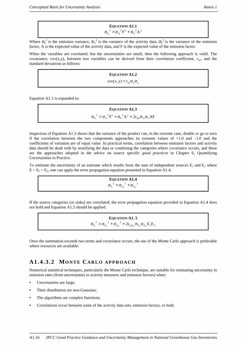
Conceptual Basis for Uncertainty Analysis Annex 1
IPCC Good Practice Guidance and Uncertainty Management in National Greenhouse Gas InventoriesA1.16
EQUATION A1.122
F22
A2
E AF σ+σ=σ
Where σE2 is the emission variance, σA
2 is the variance of the activity data, σF2 is the variance of the emission
factor, A is the expected value of the activity data, and F is the expected value of the emission factor.
When the variables are correlated, but the uncertainties are small, then the following approach is valid. Thecovariance, cov(x,y), between two variables can be derived from their correlation coefficient, rxy, and thestandard deviations as follows:
EQUATION A1.2
yxxyr)y,xcov( σσ=
Equation A1.1 is expanded to:
EQUATION A1.3
AFr2AF FAAF22
F22
A2
E σσ+σ+σ=σ
Inspection of Equation A1.3 shows that the variance of the product can, in the extreme case, double or go to zeroif the correlation between the two components approaches its extreme values of +1.0 and –1.0 and thecoefficients of variation are of equal value. In practical terms, correlation between emission factors and activitydata should be dealt with by stratifying the data or combining the categories where covariance occurs, and theseare the approaches adopted in the advice on source specific good practices in Chapter 6, QuantifyingUncertainties in Practice.
To estimate the uncertainty of an estimate which results from the sum of independent sources E1 and E2 whereE = E1 + E2, one can apply the error propagation equation presented in Equation A1.4.
EQUATION A1.42
E2
E2
E 21σ+σ=σ
If the source categories (or sinks) are correlated, the error propagation equation provided in Equation A1.4 doesnot hold and Equation A1.5 should be applied.
EQUATION A1. 521EEEE
2E
2E
2E EEr2
212121σσ+σ+σ=σ
Once the summation exceeds two terms and covariance occurs, the use of the Monte Carlo approach is preferablewhere resources are available.
A1.4 .3 .2 MO N T E CA R L O A P P R O A C H
Numerical statistical techniques, particularly the Monte Carlo technique, are suitable for estimating uncertainty inemission rates (from uncertainties in activity measures and emission factors) when:
• Uncertainties are large;
• Their distribution are non-Gaussian;
• The algorithms are complex functions;
• Correlations occur between some of the activity data sets, emission factors, or both.

Annex 1 Conceptual Basis for Uncertainty Analysis
IPCC Good Practice Guidance and Uncertainty Management in National Greenhouse Gas Inventories A1.17
Uncertainties in emission factors or activity data or both are often large and may not have normal distributions. Inthese cases, it may be difficult or impossible to combine uncertainties using the conventional statistical rules.Monte Carlo analysis can deal with this situation. The principle is to perform the inventory calculation manytimes by electronic computer, each time with the uncertain emission factors or model parameters and activity datachosen randomly (by the computer) within the distribution of uncertainties specified initially by the user. Thisprocess generates an uncertainty distribution for the inventory estimate that is consistent with the inputuncertainty distributions on the emission factors, model parameters and activity data. The method is very dataand computing time intensive, but is well suited to the problem of propagating and aggregating uncertainties in anextensive system such as a national greenhouse gas inventory. More detailed descriptions and applications of thismethod are presented in Annex 3, Glossary, and in Bevington and Robinson (1992), Manly (1997) and Cullenand Frey (1999).
A1.4.4 Propagation of uncertainties in the wholeinventory
The task of propagation of uncertainties in the inventory, after the individual uncertainties for each class ofemission are estimated, is simpler than the task of propagation of uncertainties in algorithms, because onlyaddition and subtraction are used in aggregating the emissions and uptakes.
In aggregating uncertainties, two different processes occur. Firstly, there is the aggregation of emissions of asingle gas which obeys the rules of propagation of uncertainties already discussed. The other case is theaggregation of uncertainties from several gases. In this case, the emissions and uptakes must be reduced to acommon scale, and the process for this is the use of global warming potentials (GWPs). However, for the gasesnitrogen oxides (NOx), carbon monoxide (CO), and volatile organic compounds (VOCs) there is no IPCCaccepted GWP. Consequently, the emissions and uptakes of these gases cannot be included in an aggregateduncertainty for an emissions inventory. Furthermore, it should be kept in mind that GWP values have a ratherimportant uncertainty associated with them and that an overall scientific appraisal of the total equivalent emissionshould take this into account.
As some of the variables to be aggregated are non-Gaussian, have large variances, and are correlated with othervariables, the use of a Monte Carlo approach to the aggregation of uncertainty is the preferred approach. Theapplication of this method to inventory uncertainty calculations is presented in Chapter 6, QuantifyingUncertainties in Practice.
There is the option, as a working approximation, to estimate the overall uncertainty in an inventory using theCentral Limit theorem (Cullen and Frey 1999). The assumptions relevant to the Central Limit theorem are:
• The number of emission and uptake terms are large;
• No single term dominates the sum;
• The emissions and uptakes are independent.
If this is the case then the sum of the variances of all the terms equals the variance of the total inventory, and thedistribution of the total emissions is normal. Thus the interval defined by approximately two standard deviationseither side of the mean is the 95% confidence interval of the inventory. As noted above this approach is a grossapproximation. Its use in aggregating uncertainties is an option for use at the Tier 1 of an inventory uncertaintysystem. The simplified spreadsheet approach to uncertainty analysis described in Chapter 6 uses this approach.
A1.4.5 Covariance and autocorrelationThe subsequent discussions assume that the uncertainty propagation calculations are carried out by a MonteCarlo procedure.
The emissions (or uptake) estimates of two components of the inventory are represented by the functions E1(t)and E2(t) where t is the year of the inventory estimate. These estimates have uncertainties represented by δ1(t) andδ2(t) respectively.
There are at least four significant sources of covariance in the overall inventory. These arise from:
• Use of common activity data for several emissions estimates (as occurs in the suite of gases fromcombustion);

Conceptual Basis for Uncertainty Analysis Annex 1
IPCC Good Practice Guidance and Uncertainty Management in National Greenhouse Gas InventoriesA1.18
• Mutual constraints on a group of emission estimates (such as a specified total fuel usage or total manureproduction which provides input to a number of processes);
• The evolution of activities and emission factors associated with new processes, technology etc. decouplingthe uncertainties from one time period to the next;
• External drivers that affect a suite of emissions or uptakes (economic, climatic, resource based).
For the purpose of calculating uncertainties, we are only interested in covariance between the uncertaintiesrepresented by δ1(t) and δ2(t). While covariance does occur between E1(t) and E2(t) and such covariance isrelevant to the issues of understanding and projecting emissions and uptakes, it is not of primary relevance to theissue of aggregating uncertainties etc. Therefore of these four sources of covariance, the first three are central todetermining uncertainties. The first source of covariance, the use of common activities over a range of inventorycomponents occurs particularly when several gases are emitted from the same process, such as in fossil fuelcombustion or biomass burning. The use of the same activity in two different emission estimates will lead to apositive covariance between two emission estimates. One effective way to remove this source of covariance is tocombine the equations into a single formula, having one activity and the sum of several emission factors(expressed in CO2 equivalent).
The second type of covariance occurs when there is a mutual constraint on a set of activities or emission factors,where a total activity is entered and proportions for each treatment pathway are prescribed to divide this activityamongst several emissions processes and algorithms. An example of this is the proportioning of animal manurebetween different manure waste management systems. In this case, the system can be over specified if allproportions and their uncertainties are solved simultaneously. The appropriate method of removing thecovariance is to leave one of the proportions unspecified, and to determine it by the difference between the otherproportions and the total fraction. This removes the necessity to specify the correlation of other terms with theresidual component. However, if there are correlations between the specified proportions or between thespecified proportions and the total activity, these need to be quantified and used in the uncertainty propagationcalculations.
The third type of covariance arises when new measurement techniques, new methods of recording data, or newtechnologies remove existing uncertainties and introduce new uncertainties, reducing the degree ofautocorrelation of the series over time. Autocorrelations will be high when technology, measurement techniquesand the gathering of statistics are unchanging, and low when they change. Engineering and social sciences have awealth of information to contribute on these rates of change (Grübler et al., 1999). Now that the records ofnational inventories are approaching a decade in length, there is a need for analysis of these covariances.
A1.4.6 Systematic compilation of uncertainty ininventory components
The key features of good practice for the determination of uncertainty in an individual greenhouse gas emissionor uptake in an inventory have been presented in the previous sections. These are presented in Box A1.2.
There is need for revision of the IPCC standard reporting tables to include information on uncertainties. In thesummary tables, the information recorded could be limited to confidence intervals with limits at 2.5% and 97.5%respectively. The full information described in Boxes A1.1 and A1.2 should be recorded. The practice ofuncertainty analysis in inventories is presented in detail in Chapter 6, Quantifying Uncertainties in Practice.
A1.5 APPLICATIONS
A1.5.1 Signif icance of year to year differences andtrends in inventories
A major component of uncertainty analysis for inventories is the determination of year to year and longer-termdifferences in national emissions.
If two years, t1 and t2, in a time series are considered, the difference in the total emissions between these yearscan be represented using the symbols defined in Section A1.4.5 above, by:

Annex 1 Conceptual Basis for Uncertainty Analysis
IPCC Good Practice Guidance and Uncertainty Management in National Greenhouse Gas Inventories A1.19
EQUATION A1.6)t(E)t(E)tt(E 2121 −=−∆
and the variance of the difference is defined by:
EQUATION A1.7)E,Ecov(2 21
2E
2E
2E 21
δδ−σ+σ=σ∆
or
EQUATION A1.8
212121 EEEE2E
2E
2E r2 σσ−σ+σ=σ δδ∆
Where
E1 = E(t1)E2 = E(t2)
Thus if the autocovariance or autocorrelation function of the estimated uncertainties in the inventory is known,then the significance of year to year differences can be determined. (Note that the term autocovariance is toautocorrelation as covariance is to correlation.) To estimate the correlation of the uncertainty between years inthe total inventory, one may consider the addition of two autocorrelated series representing two of the manyuncertainty components of the inventory. The autocovariance of the combined series includes theautocovariances of the individual terms plus a component to allow for the time lagged covariance between thetwo components of the inventory. For any evaluation beyond two terms, the use of a Monte Carlo analysis isrecommended.
BOX A1.2KEY FEATURES OF GOOD PRACTICE FOR THE DETERMINATION OF UNCERTAINTY IN EMISSION AND UPTAKE
ESTIMATES
(i) Use of available observations and expert judgement to determine uncertainty in inputquantities;
(ii) Systematic and transparent recording of this input data;
(iii) Examination of the available emission data to determine if representative sampling hasoccurred;
(iv) Design of further sampling and revision of parameters, default values and algorithms forkey source categories if representative sampling has not taken place;
(v) Use of sectoral good practice guidelines to choose a probability density function torepresent the data;
(vi) Evaluation of any significant correlations (covariances) between input quantities;
(vii) Propagation of uncertainties by the approximation method if the uncertainties are smalland have Gaussian distributions; otherwise
(viii) Propagation of uncertainties by Monte Carlo method where resources are available; and
(ix) Recording of uncertainty.
Enting (1999) has presented a similar analysis for the uncertainty in the trend in a quantity over a specified timeinterval. As an example, consider emissions E(t), E(t + ∆t), in two different years of a time-series separated by ∆tyears. The variance of the trend over this time period is given by:
EQUATION A1.9))t(r1(2)Evar( E
2E ∆−σ=∆ δ

Conceptual Basis for Uncertainty Analysis Annex 1
IPCC Good Practice Guidance and Uncertainty Management in National Greenhouse Gas InventoriesA1.20
This demonstrates that the uncertainty in the emission trend is smaller for positively autocorrelated estimateduncertainties, than for random uncertainties of equivalent size. There is a need for studies on autocorrelations ofestimated uncertainties in inventories as well as of cross correlations of estimated uncertainties within oneinventory year and between subsequent inventory years for related emissions and uptakes.
A1.5.2 Splicing of methodsIn some cases as the compilation of national inventories continue, there will be a need to change the algorithmused for the calculation of a particular emission or uptake. This may come about either because of improvedknowledge about the form of the algorithm or because of some change in the availability of activity data. In thesecases, the best approach is to recalculate previous years’ inventories using the new methods. In some cases, thiswill not be possible, and some means of ‘splicing’ or combining estimates prepared using different approachesinto a consistent time series will be required. The statistical theory underlying good practice is described below,and practical guidance on how to apply this in inventories is found in Chapter 7, Methodological Choice andRecalculation. The emissions (or uptake) estimates by the two methods are represented by the functions P(t) andQ(t) where t is the year of the inventory estimate. In any particular year when both estimates are available, therewill be a difference, and the task of splicing is to examine the difference. There are three likely possibilities: thetwo emissions estimates may differ by a constant amount, the two emissions estimates may be proportional toeach other, or, they may be related by both a constant difference and a proportional term. In the case analysedhere, the near constant difference is considered. (A similar analysis can be performed for the two other cases. Infact with the third case, a form of linear regression analysis is appropriate.)
The uncertainty in the difference between the two emission estimates at time t can be expressed as:
EQUATION A1.10
uncertainty = )t(QP∆δ −
where )t(Q)t(P)t(QP −=∆ −
The ideal situation is to determine this difference for many years, along with the uncertainty of the meandifference taking into account the uncertainties in P and Q. An overbar indicates the multiyear average of thedifference over the years t1–t2 and δ indicates the uncertainty of this mean difference. In this case, an acceptableseries of estimates can be made up by splicing the series P(t) and Q(t) by correcting Q(t) back to P(t) by adding
QP−∆ (t) as averaged over the period t1 to t2. A change in the estimation technique can be either an improvementor a diminishment in the quality of an estimate. If it is demonstrated that Q(t) is an improvement then Q(t)corrected back to P(t) should be used as long as possible. That is P(t) should be used up until t1, andQ(t) + QP−∆ (t) thereafter. Conversely, if P(t) is preferred, it should be used up until t2 etc.
In practice in a national inventory, three situations may arise. There may be no years of overlap between P(t) andQ(t); there may be a limited number of years of overlap which are inadequate for the process of refinement of thedifference between the two series as discussed above; and there may be sufficient number of years of overlap.
In the first two cases, some additional information is required to determine the effectiveness of the splicing.Several approaches may be possible. These are:
• Identify other locations (countries) where very similar time series exist and use these data to develop a globalor regional estimate of the mean difference QP−∆ (t) gathering all available data until δ QP−∆ (t) decreases toan acceptably small uncertainty, or all data sources are exhausted.
• When all data sources are exhausted and δ QP−∆ (t) is still above the cut off criterion, accept the time seriesnoting that the time series, from beginning to end has an additional uncertainty that arises because of theuncertainty in the difference between the two series.
• Where there is no overlap of data, nor any data available from elsewhere, other splicing techniques areneeded. One possibility is the use of time series techniques (Box and Jenkins, 1970) to forward forecast P(t)and to back forecast in time Q(t) and to see if in the immediate years around the splice, these forecasts agreewith the other data set to within the 95% confidence interval. If so the splice could be accepted, if not then adiscontinuity in the emissions (or uptake) estimates would have to be recorded. In both these cases, the

Annex 1 Conceptual Basis for Uncertainty Analysis
IPCC Good Practice Guidance and Uncertainty Management in National Greenhouse Gas Inventories A1.21
uncertainty applied throughout the time series would, at minimum, be the combined uncertainty arising fromeach of the estimates P(t) and Q(t).
Practical approaches to splicing are discussed in Chapter 7, Methodological Choice and Recalculation.
A1.5.3 Sensit ivity analyses and the sett ing ofnational inventory research priorit ies
Given the objective of reducing uncertainties in an inventory, priorities for further research should be establishedbased on three main characteristics:
• The importance of the source category or sink;
• The size of the uncertainty in the emission and uptake;
• The research cost and the expected benefit, measured as an overall reduction in the uncertainty of theinventory.
The importance of the source category should be established using the criteria described in Chapter 7,Methodological Choice and Recalculation. Among source categories of equal magnitude, priority should begiven to those with larger uncertainties or greater effect on the trend.
For each source category, the options for research will depend on the origins of the uncertainty. In most cases,there are a number of variables that determine the activity and the emission factor. Priority should be given tothose quantities which influence the overall uncertainty most. Among the research options, further stratificationof the emissions and uptakes can lead to great benefit. In fact, many current default values are defined for a widerange of conditions which necessarily leads to large confidence intervals.
In the present context, the research cost includes financial cost, time involved and other components that cannotalways be quantified.
There are sophisticated computational techniques for determining the sensitivity of a model (such as aninventory) output to input quantities. These methods rely on determining a sensitivity coefficient, λ, that relatesthe aggregated emissions ET to an input quantity (or parameter) which in this case is represented by a. Thesemethods determine the coefficient as:
Equation A1.11a/ET ∂∂=λ
Some software packages for Monte Carlo analyses have an option for such analysis. This approach has been usedfor atmospheric chemical systems involving tens to hundreds of chemical reactions (NAS, 1979; Seinfeld andPandis, 1998). However, one difference between these chemical models and greenhouse gas inventories is thestate of knowledge. Chemical models generally represent a closed system with conservation of mass, well-defined relationships and a suite of rate constants that mostly have been well quantified. There is much lessknowledge about the extent of interactions, and values of quantities and parameters in greenhouse gasinventories.
There are other approaches that may fill the need for providing input on measurement and research priorities forinventory development. It is possible to develop simpler methods, using broad assumptions, to provide indicationof research priorities. The advantage of these simpler schemes is that they can be used by all inventory compilers.Such information on research and measurement priorities arises from the evaluations of representative samplingas discussed in Section A1.4.2, Representative sampling, algorithms and covariances, the uncertainty analysis inChapter 6, Quantifying Uncertainties in Practice, and Chapter 7, Methodological Choice and Recalculation, andfrom the good practice guidance for each sector (see Chapters 2 to 5). These various inputs combined with theexpert judgement of inventory compilers provide the best guide to priorities for inventory development.
A1.6 RESEARCH REQUIREMENTSWhile some of the assumptions that underpin IPCC inventories are self evident and already have been examined,the systematic investigation of the set of assumptions that underpin these inventories would facilitate a structured

Conceptual Basis for Uncertainty Analysis Annex 1
IPCC Good Practice Guidance and Uncertainty Management in National Greenhouse Gas InventoriesA1.22
approach to the identification of uncertainties and the design of experiments to test and refine these assumptions.This work includes issues of definition and the theoretical basis of emission algorithms. Such work wouldstrengthen the coupling of understanding, and exchange of information, between IPCC inventories and studies ofthe global cycles of trace gases incorporated in IPCC Working Group 1, to the benefit of both activities.
One currently unresolved aspect of the reporting of emissions and uptakes is the number of significant digitsrecorded (numerical precision). The approach in ISO (1993) is that the numerical values of the estimate and itsstandard deviation should not be given with an excessive number of digits. The Canadian National GreenhouseGas Inventory has adopted the practice of only reporting data to the number of significant digits commensuratewith the uncertainty of the inventory estimates. If care is taken to maintain this association throughout theinventory, it is possible to clearly visualise the uncertainty of the values and the difference between theuncertainty associated with the emissions from each source category. The other approach is to define theminimum unit for reporting as a fixed quantity, then inventories from all countries and all components of theseinventories are reported with the same numerical unit. In practical terms there are probably advantages in thisapproach for ease of auditing the tables, but this issue will require further discussion.
REFERENCESBevington, P. R. and Robinson, D. K. (1992). Data Reduction and Error Analysis for the Physical Sciences.
WCB/McGraw-Hill Boston USA, p. 328.
Bouwman, A.F. (1996). ‘Direct emission of nitrous oxide from agricultural soils’. Nutrient Cycling inAgroecosystems, 46, pp. 53-70.
Box, G.E.P. and Jenkins, G.M. (1970). Time Series Analysis forecasting and control. Holden-Day, SanFrancisco, USA, p. 553.
Cochran, W.G. (1963). Sampling Techniques. 2nd edition, John Wiley & Sons Inc., New York, p. 411.
Cullen, A.C. and H.C. Frey, H.C. (1999). Probabilistic Techniques in Exposure Assessment, Plenum PublishingCorp., New York, USA, p. 335.
Eggleston, S. (1993). Cited in IPCC (1996) Revised Guidelines for National Greenhouse Gas Inventories, op.cit.
Enting, I.G. (1999). Characterising the Temporal Variability of the Global Carbon Cycle. CSIRO TechnicalPaper No 40, CSIRO Aspendale, Australia, p. 60.
Grübler, A., N. Nakićenović, N. and Victor D.G. (1999). ‘Dynamics of energy technologies and global change’,Energy Policy, 27, pp. 247-280.
IPCC (1996). Revised 1996 IPCC Guidelines for National Greenhouse Gas Inventoires: Volumes 1, 2 and 3.J.T. Houghton et al., IPCC/OECD/IEA, Paris, France.
ISO (1993). Guide to the Expression of Uncertainty in Measurement. International Organisation forStandardiszation, ISBN 92-67-10188-9, ISO, Geneva, Switzerland, p.101.
Mandel, J. (1984). The Statistical Analysis of Experimental Data. Dover Publications New York, USA, p. 410.
Manly, B.F.J. (1997). Randomization, Bootstrap and Monte Carlo Methods in Biology. 2nd edition, Chapman &Hall, p. 399.
NAS (1979). Stratospheric Ozone Depletion by Halocarbons: Chemistry and Transport. Panel on StratosphericChemistry and Transport, National Academy of Sciences, Washington D.C., USA, p.238.
Robinson, J.R. (1989). ‘On Uncertainty in the Computation of Global Emissions for Biomass Burning’. ClimaticChange, 14, pp. 243-262.
Seinfeld, J.H. and Pandis, S.N. (1998). Atmospheric Chemistry and Physics. John Wiley and Sons, New York,USA, p. 1326.
Subsidiary Body for Scientific and Technological Advice (SBSTA), United Nations Framework Convention onClimate Change (1999). National Communications from Parties included in Annex 1 to the Convention,Guidelines for the Preparation of National Communications, Draft conclusions by the Chairman.FCCC/SBSTA/1999/L.5, p. 17.

Annex 2 Verification
IPCC Good Practice Guidance and Uncertainty Management in National Greenhouse Gas Inventories A2.1
A N N E X 2
VERIFICATION

Verification Annex 2
A2.2 IPCC Good Practice Guidance and Uncertainty Management in National Greenhouse Gas Inventories
CO-CHAIRS, EDITORS AND EXPERTS
Co-chairs of the Expert Meeting on Cross-sectoral Metholodogies forUncertainty Estimation and Inventory QualityTaka Hiraishi (Japan) and Buruhani Nyenzi (Tanzania)
REVIEW EDITOR
Leo Meyer (Netherlands)
Expert Group: Checks and Verification at National and InternationalLevelCO-CHAIRS
Mike Woodfield (UK) and Faouzi Senhaji (Morocco)
AUTHORS OF BACKGROUND PAPERS
Jos Olivier (Netherlands), Wilfried Winiwarter (Austria), and Jean-Pierre Chang (France)
CONTRIBUTORS
William Breed (USA), Zhenlin Chen (China), Riccardo De Lauretis (Italy), Eilev Gjerald (Norway), MichaelStrogies (Germany), Susan Subak (USA), Kiyoto Tanabe (IPCC-NGGIP/TSU), Karen Treanton (IEA), andAndre van Amstel (Netherlands)

Annex 2 Verification
IPCC Good Practice Guidance and Uncertainty Management in National Greenhouse Gas Inventories A2.3
C o n t e n t s
ANNEX 2 VERIFICATION
A2.1 INTRODUCTION............................................................................................................................ A2.4
A2.1.1 National level........................................................................................................................... A2.4
A2.1.2 Additional international comparative tools.............................................................................. A2.5
A2.1.3 Comparisons with atmospheric measurements at local, regional and global scales ................. A2.8
A2.1.4 Comparisons with international scientific publications, global or regional budgets and source trends ..................................................................................................................... A2.9
A2.2 PRACTICAL GUIDANCE FOR VERIFICATION OF EMISSIONS INVENTORIES.................. A2.9
A2.2.1 National inventories................................................................................................................. A2.9
A2.2.2 Aggregated global or regional inventories............................................................................. A2.10
A2.3 REPORTING.................................................................................................................................. A2.10
REFERENCES ......................................................................................................................................... A2.11
F i g u r e s
Figure A2.1 Illustrative Plot for an Inter-country Comparison of Emission Factors......................... A2.7
Figure A2.2 Illustrative Plot for an Inter-country Comparison of Emission Factorsand their Uncertainties .................................................................................................. A2.7

Verification Annex 2
A2.4 IPCC Good Practice Guidance and Uncertainty Management in National Greenhouse Gas Inventories
ANNEX 2 VERIFICATION
A2.1 INTRODUCTIONVerification processes are, in the present context, intended to help establish an inventory’s reliability. Theseprocesses may be applied at either national or global levels of aggregation and may provide alternativeinformation on annual emissions and trends. The results of verification processes may:
(i) Provide inputs to improve inventories;
(ii) Build confidence in emissions estimates and trends;
(iii) Help to improve scientific understanding related to emissions inventories.
Verification processes may also enhance international cooperation in improving inventory estimates.
There are different approaches to verification. One approach is to evaluate emissions estimates and trends, forexample, as part of the United Nations Framework Convention on Climate Change (UNFCCC) review ofemissions inventories. Another approach entails an evaluation of aggregate inventories on a global or regionalbasis, with the objective of providing further scientific insight.
A number of options or tools for verification are discussed in this Annex. Their application, as well as the typesof information needed, will vary according to the role and intention of the verification process. Internationalverification of inventories may include comparisons with international or independently compiled activity data,emissions factors, uncertainty estimates, atmospheric measurements, and global or regional budgets and sourcetrends. International verification will usually occur following inventory preparation, including the qualityassurance/quality control (QA/QC) process (see Section A2.2.1, National Inventories, in this Annex and Chapter8, Quality Assurance and Quality Control). International verification may occur in the absence of nationalverifications. Verification activities require resources, time and technical and intellectual expertise.
Verification processes and results should be reported systematically and in a timely manner, in order to providefeedback to national inventory teams, and to the international community, as appropriate, depending on the roleand reason for verification.
Techniques for Verif icat ion
Verification techniques include internal quality checks, inventory inter-comparison, comparison of intensityindicators, comparison with atmospheric concentrations and source measurements, and modelling studies. In allcases, comparisons of the systems for which data are available and the processes of data acquisition should beconsidered along with the results of the studies. These techniques, and their applicability at the national andinternational level, are discussed below.1
A2.1.1 National LevelVerification procedures can be conducted on parts of national inventories as part of the QA/QC process (seeChapter 8, Quality Assurance and Quality Control), or on parts or the whole inventory as a separate exercise.
A2.1 .1 .1 CO M P A R I S O N S W I T H O T H E R N A T I O N A L E M I S S I O N SD A T A
Comparisons with other, independently compiled, national or regional emissions estimates are a quick option toverify completeness, approximate emission levels, or allocations to source categories or sub-source categories.The availability of such independently compiled inventories will vary, but possible resources include state orprovincial inventories, as well as inventories prepared independently by research organisations. Specific steps fornational comparison are similar to those for comparisons with international data, as described in Section A2.2.1,National Inventories.
1 Some of the options are described in more detail in EEA (1997), Lim et al. (1999a, b) and Van Amstel et al. (1999).

Annex 2 Verification
IPCC Good Practice Guidance and Uncertainty Management in National Greenhouse Gas Inventories A2.5
A2.1 .1 .2 DI R E C T S O U R C E T E S T I N G
On-line stack measurements, in-plume measurements, remote measurements, and tracers have been used fordirect testing of sources. All these approaches allow the direct attribution of observed concentrations to theemissions from a certain source. So long as it is representative, the uncertainty associated with the measurementand emission calculations in direct source testing is often considered to be lower than the uncertainty of inventoryemissions estimates that may have been calculated by other methods. See Chapter 8, Quality Assurance andQuality Control, Section 8.7.1.3, Direct Emission Measurements, for further discussion of this topic.
A2.1 .1 .3 CO M P A R I S O N W I T H N A T I O N A L S C I E N T I F I C A N D O T H E RP U B L I C A T I O N S
Although the inventory agency is responsible for the compilation and submission of the national greenhouse gasinventory, there may be other independent publications of relevance (e.g. scientific and technical literature).Examining such literature sources may identify areas for further research and inventory improvement.
A2.1.2 Additional international comparative toolsComparison of national greenhouse gas inventories with international data sets may be an independent means toverify inventory estimates. Several types of comparisons can be made, including comparisons with independentlycompiled bottom-up emissions estimates, comparisons with atmospheric measurements, comparisons withinternational scientific literature sources, and comparisons with global or regional budgets. Comparisons withinventories from other countries enable cross-checking of assumptions regarding the use of emission factors,completeness of source categories and overall approaches. In addition to comparisons with single countryemissions inventories, it is possible to make more systematic comparisons for larger groups of countries.
A2.1 .2 .1 BO T T O M-U P C O M P A R I S O N S
For a given source category, different types of bottom-up comparisons can be performed in parallel. Thesecomparisons can examine overall emission levels, emission factors, or activity data. The broad types can include:
• Comparisons with other independently compiled datasets, in order to check for completeness, magnitude,and source allocation;
• Inter-country comparisons in which input data (i.e. activity levels, aggregated emission factors or otherfactors used in emission calculations) are compared for different countries for the same year;
• Inter-country comparisons in which trends in emissions or input data are compared for different countries.
These different types of comparisons can also assist in evaluating the uncertainty estimates of nationalinventories and global emission inventories, and evaluating differences at the country level. These comparisonprocesses do not always represent verification of the data themselves, but instead verification of the reliabilityand the consistency of data (e.g. in trends and between countries). They can enable reviewers to identifyinconsistencies or questions for which more detailed data verification may need to be performed. The time thatinventory agencies are able to spend on these independent verification activities will depend upon the resourcesavailable and an assessment of the value of these activities compared to other means of improving inventoryquality.
Several examples of the types of comparisons are described below:
• Comparisons of Top-down and Bottom-up Estimates: For carbon dioxide (CO2) from fossil fuel combustion,a reference calculation based on apparent fuel consumption per fuel type is mandatory according to theRevised 1996 IPCC Guidelines for National Greenhouse Gas Inventories (IPCC Guidelines). This type oftop-down completeness and order-of-magnitude check may also be applicable in other cases where theinventory is based on a bottom-up approach. In cases where emissions are calculated as the sum of sectoralactivities based on the consumption of a specific commodity (e.g. fuels or products like hydrofluorocarbons(HFCs), perfluorocarbons (PFCs) or sulfer hexafluoride (SF6)), the emissions could be estimated usingapparent consumption figures (e.g. national total production + import – export ± stock changes).

Verification Annex 2
A2.6 IPCC Good Practice Guidance and Uncertainty Management in National Greenhouse Gas Inventories
• Comparisons of National Emission Inventories with Independently Compiled, International Datasets: Someglobal databases already exist. For example, CO2 emissions estimates associated with the combustion offossil fuel are compiled by the International Energy Agency (IEA) and the Carbon Dioxide Information andAnalysis Centre (CDIAC). Global total anthropogenic inventories of all greenhouse gases are compiled bythe Global Emission Inventory Activity (GEIA, a component of IGAC/IGBP) and the Emission Database forGlobal Atmospheric Research (EDGAR), as compiled by TNO Institute of Environmental Science andNational Institute of Public Health and the Environment (RIVM) in close cooperation with GEIA (IEA,1999; Marland et al., 1994; Graedel et al., 1993; Olivier et al., 1999). These comparisons can assist inchecking completeness, consistency, source allocation and accuracy to within an order of magnitude.However, when evaluating the results of these comparisons, it should be remembered that the various datasources are often not completely independent of each other or from the data set used to calculate the nationalinventory. For example, EDGAR starts with IEA energy data to calculate CO2 emissions from fuelcombustion and CDIAC and GEIA datasets start with UN energy data. In addition, even the IEA and UNenergy data are not completely independent. In order to avoid duplication of work, the IEA and the UnitedNations cooperate in the exchange of data and use common questionnaires for some countries.
• Comparisons of Activity Data with Independently Compiled Datasets: Similar comparisons may be madeusing the underlying activity data to check completeness and order-of-magnitude. These underlying data maybe compared with independently compiled international statistics (e.g. maintained by the IEA, and theUnited Nations Food and Agriculture Organization). One should not, however, expect to find exact matchessince the activity data used by the inventory agency may be taken from different data sources or be adifferent version to that used in the national data collected by international organisations; for examples seeSchipper et al. (1992). When checking activity data, indicators could be defined for the purpose ofinternational comparison (e.g. activity rate per inhabitant, per employee, per unit of GDP, per number ofhouseholds or per number of vehicles, according to the source sectors). This could enable order-of-magnitude checks and indicate outliers that may be caused by data input or calculation errors.
• Comparisons of Emission Factors Between Countries: Different kinds of comparisons can be combined inpractice. For example, between-country emission factor comparisons can be combined with historic trendsby plotting, for different countries, the reference year data (e.g. 1990), the more recent year data, and theminimum and maximum values. This analysis could be made for each source category and possibleaggregations. Sub-source categories such as fuel types may also be included when relevant (see Figure A2.1,Illustrative Plot for an Inter-country Comparison of Emission Factors). Comparisons between countries canalso be made using implied emission factors (which are top-down ratios between emissions estimates andactivity data). This type of comparison may enable outlier detection based on the statistical distribution ofvalues from the sample of countries considered, bearing in mind that differences in national circumstancescan significantly affect the implied emission factors. Since implied emission factors are ratios of emissions toactivity data, comparisons based on them should help verify both the emission factors and the activity data inthe original calculation. Finally, a comparison with the IPCC Tier 1 default values and with literature valuesmay be informative in establishing the comparability or country-specificity of the emission factors used.
• Comparisons Based on Estimated Uncertainties: Comparisons based on the estimated uncertainties ofemission factors, when such data are available, can also be useful. For example, Figure A2.2, Illustrative Plotfor an Inter-country Comparison of Emission Factors and their Uncertainties, shows on a single plot currentyear’s emission factor and the related uncertainty range for different countries. This can be done for a givensource category and, when relevant, sub-source categories such as different fuel types. This type ofcomparison may help to identify data outliers where uncertainty ranges do not overlap.
• Comparisons of Emission Intensity Indicators Between Countries: Emission intensity indicators may becompared between countries (e.g. emissions per capita, industrial emissions per unit of value added,transport emissions per car, emissions from power generation per kWh of electricity produced, emissionsfrom dairy ruminants per tonne of milk produced). These indicators provide a preliminary check andverification of the order of magnitude of the emissions. It is not expected that emission intensity indicatorswill be correlated across countries. Different practices and technological developments as well as the varyingnature of the source categories will be reflected in the emission intensity indicators. However, these checksmay flag potential anomalies at country or sector level.2
2 More examples for energy indicators can be found in Schipper and Haas (1997) and Bossebeuf et al. (1997).

Annex 2 Verification
IPCC Good Practice Guidance and Uncertainty Management in National Greenhouse Gas Inventories A2.7
F i g u r e A 2 . 1 I l l u s t r a t i v e P l o t f o r a n I n t e r - c o u n t r y C o m p a r i s o n o fE m i s s i o n F a c t o r s
F i g u r e A 2 . 2 I l l u s t r a t i v e P l o t f o r a n I n t e r - c o u n t r y C o m p a r i s o n o fE m i s s i o n F a c t o r s a n d t h e i r U n c e r t a i n t i e s
Emissionfactors(from
referenceto current
year)(unit) 90
97
country1
90
97
country2
97
90
country3 countries
90/97
country4
90
97
country5
90/97
country6
Source category/sub-source category : xxxPollutant : xxx
N.B. : The E.F. range for a given country relates here to the minimum and maximum E.F. during the period 90-97.
Emissionfactors anduncertainty
ranges(unit)
country1 country2 country3 countriescountry4 country5 country6
Source category/sub-source category : xxxPollutant : xxx
N.B. : The E.F. range for a given country relates here to the uncertainty range of the current E.F.
Year : xxx

Verification Annex 2
A2.8 IPCC Good Practice Guidance and Uncertainty Management in National Greenhouse Gas Inventories
A2.1 .2 .2 CO M P A R I S O N S O F U N C E R T A I N T Y E S T I M A T E SB E T W E E N C O U N T R I E S
Chapter 6, Quantifying Uncertainties in Practice, describes how to estimate and report uncertainties. Theuncertainty estimates developed for various source categories may be compared in several ways, including:
• Comparing the uncertainty estimates of various source categories and gases within a country’s inventory;
• Comparing the uncertainty of a given gas for specific source categories between countries;
• Comparing the uncertainty estimates reported in the national inventory with those provided in relatedregional or other national inventories or other documents used for verification purposes.
Many factors influence the uncertainty estimates for different gases in different source categories and these arenot expected to be identical. However, such comparisons may alert the inventory agency to possible areas forimprovement.
A2.1.3 Comparisons with atmospheric measurementsat local , regional and global scales
For some regions, emission source categories, or compounds, comparisons with atmospheric measurements mayprovide useful information on the validity of the emissions estimates in the context of overall atmospheric trends.Several options may be employed, including:
• Local and Regional Atmospheric Sampling: At a given site, background concentrations may be inferred fromlow concentration levels, and enhanced concentrations (plumes) from high concentration levels.Measurements can be performed at several fixed sites upwind and downwind thus allowing the comparisonof measured concentrations with modelled concentrations. In terms of emission assessment, however, it ismore appropriate to perform inverse modelling (i.e. estimate emissions from measured concentrations). Asan example, markers (13C) have been used to assess methane (CH4) emissions (Levin et al., 1999) inatmospheric sampling. Such methods are not limited to areas defined by national boundaries. Indeed, theyare best suited to regions where emissions are concentrated in a small area. As industrial and populationcentres are frequently situated at both sides of a national boundary, an evaluation for just one country maynot be possible because emissions can only be assessed for the whole area. In such cases, the methods areonly useful at a bilateral or international level.
• Continental Plumes: A strong difference between source and non-source (sink) regions may generally befound between a continent and an ocean. Routine measurements may be performed close to an ocean, atoffshore islands, or on ships. The difference between background air concentrations and the offshore plumeconcentrations, taking advantage of wind vector analysis or trajectory analysis, may provide an indication ofemissions on a broad scale. For example, a number of greenhouse gases, including chlorofluorocarbons(CFCs), nitrous oxide (N2O) and CH4 from the European continental plume, have been detected at MaceHead, Ireland. These results have then been used for subsequent quantification of the European emissionsource strength by inverse modelling (Derwent et al., 1998a, b; Vermeulen et al., 1999).
• Satellite Observations: Satellite observations allow users to retrieve quasi-continuous concentration profilesfor all or part of the globe.
• Global Dynamic Approaches: Trends over time in the atmospheric concentration of particular compoundsmay also indicate a change in the global balance between sources and sinks. This may be particularly usefulwhere the background concentration of the gas in the atmosphere is low. Such approaches have been takenfor CH4 (Dlugokencky et al., 1994) and SF6 (Maiss and Brenninkmeijer, 1998).
These methods allow a large proportion of global emissions to be covered and monitoring is possible on a routinebasis. However, it is almost impossible to trace emissions back to individual sources or source categories if theiremissions do not contain some sort of ‘fingerprint’ that characterises them. This ‘fingerprint’ may be a specifictype of carbon isotope in the case of CO2 and CH4 emissions from fossil fuels, or a typical temporal profile(seasonality or diurnal variation) or zonal variation (e.g. latitudinal distribution).
Annex 2 Verification
IPCC Good Practice Guidance and Uncertainty Management in National Greenhouse Gas Inventories A2.9
A2.1.4 Comparisons with international scientif icpublications, global or regional budgets andsource trends
The international scientific literature may provide other estimates or analyses to compare with national inventoryestimates. Comparison of these estimates with such literature is a valuable check on the quality of the officialnational inventory that can be used when comparing or integrating the greenhouse gas emissions of variouscountries.
Comparisons of national inventories with independently compiled global inventories and with global or regionalemission levels included as part of a more comprehensive analysis are a means to update global budgets orprovide feedback to national inventory developers or both. Provided that sufficient information is available onspatial and temporal distribution of the sources, including natural sources, it may be possible to trace the reasonsfor inconsistencies between different reports of emissions for major sources (Heimann, 1996, for CO2; Janssen etal., 1999, and Subak, 1999, for CH4; Bouwman and Taylor, 1996, for N2O).
A2.2 PRACTICAL GUIDANCE FORVERIFICATION OF EMISSIONSINVENTORIES
There is value in independent verification of individual national greenhouse gas inventories at the internationallevel (e.g. inter-country comparisons). Such verification activities could serve the following purposes:
• Support the national verification activities;
• Improve efficiency by avoiding duplication of effort at the national level;
• Provide input to evaluation of the IPCC Guidelines;
• Inform the public, scientists and government reviewers.
A2.2.1 National inventoriesIf an independent verification is considered a valuable means for improving inventory estimates, it would begood practice to have the following:
• Availability of sufficient independent expertise;
• National inventory report;
• Uncertainty estimates and QA/QC documentation included in the report;
• Reports of existing national verifications.
It is also useful to identify gaps in the inventory prior to undertaking any verification process.
The list in Box A2.1, Verification of a National Inventory, summarises and ranks the tools in order ofapproximate ease of implementation. The best combination for a particular user will depend upon the availabledata, and resource constraints (e.g. funding, time, expertise).

Verification Annex 2
A2.10 IPCC Good Practice Guidance and Uncertainty Management in National Greenhouse Gas Inventories
BOX A2.1VERIFICATION OF A NATIONAL INVENTORY
A. Checks:
• Check for discontinuities in emission trends from base year (usually 1990) to end year.
B. Comparisons of emissions and other such features:
• Compare the Reference Approach for CO2 emissions from fuel combustion with otherapproaches.
• Compare inventory emissions estimates by source category and gas against independentlycompiled national estimates from international databases.
• Compare activity data against independently compiled estimates and perhaps activity data fromcountries with similar source categories and sectors.
• Compare (implied) emission factors for source categories and gases with independentestimates and estimates from countries with similar source categories and sectors.
• Compare sector intensity estimates of selected source categories with estimates from othercountries with similar source categories and sectors. If necessary, calculate emission intensityestimates based on international statistical compendia.
C. Comparisons of uncertainties:
• Compare uncertainty estimates with those from reports of other countries and the IPCC defaultvalues.
D. On-site measurements:
• Perform direct source testing on key source categories, if possible.
Some of these activities may have been conducted as part of the QA/QC processes and results may be included inthe inventory report. After the selected processes in Box A2.1 have been completed and issues to be reviewed inmore detail have been identified, the following information may also support the verification processes:
• National reports;
• Additional tools such as scientific literature on emission factors;
• Results from atmospheric sampling relevant to key source categories and sectors.
Findings should be summarised and feedback sought from the inventory agency. Findings of the verificationprocess should be made publicly available wherever possible.
A2.2.2 Aggregated global or regional inventoriesThere is also value in examining emissions inventory information between countries and as totals of groups ofcountries. Such evaluations could, for example, compare global or regional totals and trends against atmosphericconcentrations and changes in concentrations. Comparison of global or regional totals of selected sourcecategories against isotopic signature analysis may provide additional information. This type of verification mayprovide an indicative range for emissions estimates.
The explicit steps, and the data required, will be determined by the intent and scope of the verification effort andanalysis. Discrepancies identified by verification processes on aggregate national inventories and comparisonswith atmospheric concentrations may guide future priorities for research on national inventories and atmosphericscience.
A2.3 REPORTINGFor the verification process to be most useful, findings should be made publicly available.

Annex 2 Verification
IPCC Good Practice Guidance and Uncertainty Management in National Greenhouse Gas Inventories A2.11
The report should include the following items:
• What has been verified;
• How the verification was performed;
• What criteria were used for the selection of verification priorities;
• Limitations in the processes that have been identified;
• What feedback was received from external reviewers summarising key comments;
• Actions taken by the inventory agency as a result of the verification process;
• Recommendations for inventory improvements or research at an international level arising from the findings.
To facilitate use of the reports and wide dissemination, verification reports should use the common unitsrecommended by the IPCC Guidelines and the official languages of the United Nations.
REFERENCESBosseboeuf, D., Chateau, B. and Lapillonne, B. (1997). ‘Cross-country comparison on energy efficiency
indicators: the on-going European effort towards a common methodology’. Energy Policy, 25, pp. 673-682.
Bouwman A.F. and J. Taylor (1996). ‘Testing high-resolution nitrous oxide emission estimates againstobservations using anatmospheric transport model’. Global Biogeochemical Cycles, 10, pp. 307-318.
Derwent R.G., Simmonds P.G., O’Doherty S. and Ryall D.B. (1998a). ‘The impact of the Montreal Protocol onHalocarbon concentrations in Northern Hemisphere baseline and European air masses at Mace Head, Ireland,over a ten year period from 1987-1996’. Atmos. Environ., 32, pp. 3689-3702.
Derwent R.G., Simmonds P.G., O’Doherty S., Ciais P. and Ryall D.B. (1998b). ‘European source strengths andNorthern Hemisphere baseline concentrations of radiatively active trace gases at Mace Head, Ireland’. AtmosEnviron., 32, pp. 3703-3715.
Dlugokencky E.J., Steele L.P., Lang P.M. and Mesarie K.A. (1994). ‘The growth rate and distribution ofatmospheric CH4’. J. Geophys. Res., 99, pp. 17021-17043.
European Environmental Agency (EEA) (1997). Joint EMEP/CORINAIR Atmospheric Emission InventoryGuidebook. European Environmental Agency, Copenhagen.
Graedel T. E., Bates, T.S., Bouwman, A.F., Cunnold, D., Dignon, J., Fung, I., Jacob, D.J, Lamb, B.K., Logan,J.A., Marland, G., Middleton, P., Pacyna, J.M., Placet, M. and Veldt, C. (1993). ‘A compilation ofinventories of emissions to the atmosphere’. Global Biogeochemical Cycles, 7, pp. 1-26.
Heimann M. (1996). ‘Closing the atmospheric CO2 budget: inferences from new measurements of 13C/12C andO2/N2 ratios.’ IGBP Newsletter, 28, pp. 9-11.
International Energy Agency (IEA) (1999). CO2 emissions from fuel combustion 1971-1997. OECD/IEA, Paris,France. ISBN 92-64-05872-9. A diskette service with more detailed sectors/fuels is also available.
Janssen L.H.J.M., J.G.J. Olivier, A.R. van Amstel (1999). ‘Comparison of CH4 emission inventory data andemission estimates form atmospheric transport models and concentration measurements’. EnvironmentalScience & Policy, 2, pp. 295-314.
Levin I., H. Glatzel-Mattheier, T. Marik, M. Cuntz, M. Schmidt, D.E. Worthy (1999). ‘Verification of Germanmethane emission inventories and their recent changes based on atmospheric observations’. J. Geophys. Res.,104, pp. 3447-3456.
Lim B., P. Boileau, Y. Bonduki, A.R. van Amstel, L.H.J.M. Janssen, J.G.J. Olivier, C. Kroeze (1999a).‘Improving the quality of national greenhouse gas inventories’. Environmental Science & Policy, 2, pp. 335-346.
Lim, B, P. Boileau (1999b). ‘Methods for assessment of inventory data quality: issues for an IPCC expertmeeting’. Environmental Science & Policy 2, pp. 221-227.
Maiss M. and C.A.M. Brenninkmeijer (1998). ‘Atmospheric SF6: trends, sources and prospects’. Environ. Sci.Techn., 32, pp. 3077-3086.
Verification Annex 2
A2.12 IPCC Good Practice Guidance and Uncertainty Management in National Greenhouse Gas Inventories
Marland G., Andres, R.J. and Boden, T.A. (1994). ‘Global, regional, and national CO2 emissions’. In: Trends'93: A Compendium of Data on Global Change, Boden, T.A., Kaiser, D.P., Sepanski, R.J. and Stoss, F.W.(eds.), ORNL/CDIAC-65, Carbon Dioxide Information Analysis Center, Oak Ridge National Laboratory,Oak Ridge, TN, USA, pp. 505-584.
Olivier J.G.J., A.F. Bouwman, J.J.M. Berdowski, C. Veldt, J.P.J. Bloos, A.J.H. Visschedijk, C.W.M. van derMaas and P.Y.J. Zandveld (1999). ‘Sectoral emission inventories of greenhouse gases for 1990 on a percountry basis as well as on 1ox1o ’. Environmental Science and Policy, 2, pp. 241-264.
Schipper L., Meyers, S., Howarth, R.B., and Steiner, R. (1992). Energy efficiency and human activity. Pasttrends, future prospects. Cambridge University Press, Cambridge, UK.
Schipper L., R. Haas (1997). ‘The political relevance of energy and CO2 indicators – an introduction’. EnergyPolicy 25, pp. 639-649.
Subak, S. (1999). ‘On evaluating accuracy of national methane inventories’. Environmental Science Policy, 2,pp. 229-240.
Van Amstel A.R, J.G.J. Olivier and L.H.J.M. Janssen (1999). ‘Analysis of differences between nationalinventories and an Emissions Database for Global Atmospheric Research (EDGAR)’. Environmental Science& Policy, 2, pp. 275-294.
Vermeulen A.T., R. Eisma, A. Hensen, J. Slanina (1999). ‘Transport model calculations of NW-Europeanmethane emissions’. Environmental Science & Policy, 2, pp. 315-324.

Annex 3 Glossary
IPCC Good Practice Guidance and Uncertainty Management in National Greenhouse Gas Inventories A3.1
A N N E X 3
GLOSSARY

Glossary Annex 3
IPCC Good Practice Guidance and Uncertainty Management in National Greenhouse Gas InventoriesA3.2
CO-CHAIRS, EDITORS AND EXPERTS
Co-chairs of the Expert Meeting on Cross-sectoral Methodologies forUncertainty Estimation and Inventory QualityTaka Hiraishi (Japan) and Buruhani Nyenzi (Tanzania)
REVIEW EDITOR
Richard Odingo (Kenya)
AUTHORS
Milos Tichy (Czech Republic) and Simon Bentley (Australia)
REVIEWERS
Roberto Acosta (UNFCCC Secretariat), Simon Eggleston (UK), Ian Galbally (Australia), Katarina Mareckova(Slovak Republic), Thomas Martinsen (IPCC/OECD), Jos Olivier (Netherlands), Jim Penman (UK), and KristinRypdal (Norway)

Annex 3 Glossary
IPCC Good Practice Guidance and Uncertainty Management in National Greenhouse Gas Inventories A3.3
C o n t e n t s
ANNEX 3 GLOSSARY
INDEX TO THE GLOSSARY................................................................................................................... A3.4
A3.1 INTRODUCTION............................................................................................................................ A3.6
A3.1.1 Selection of entries ................................................................................................................. A3.6
A3.1.2 Formulation of entries............................................................................................................. A3.6
A3.2 GLOSSARY ..................................................................................................................................... A3.7
REFERENCES ......................................................................................................................................... A3.21

Glossary Annex 3
IPCC Good Practice Guidance and Uncertainty Management in National Greenhouse Gas InventoriesA3.4
I n d e x
A
Accuracy A3.7
Activity data A3.7
Arithmetic mean A3.7
Auto-correlation A3.7
Auto-covariance A3.8
B
Bias A3.8
Bootstrap technique A3.8
C
Central limit theorem A3.8
Coefficient of variation A3.8
Comparability A3.8
Completeness A3.8
Confidence A3.9
Confidence interval A3.9
Consistency A3.9
Correlation A3.9
Correlation coefficient A3.9
Covariance A3.10
Cumulative distribution functionSee Distribution function
D
Decision tree A3.10
Distribution function A3.10
E
Elasticity A3.10
Emission Factor A3.10
Error A3.10
Estimation A3.10
Estimator A3.11
Expectation A3.11
Expected value A3.11
Expert Judgement A3.11
Extreme value A3.11
G
Good Practice A3.11
I
Independence A3.12
K
Key source category A3.12
Kurtosis A3.12
L
Latin hypercube sampling A3.12
Law of large numbers A3.12
Linear model A3.12
Linear regression A3.12
Lognormal distribution A3.13
M
Mean A3.13
Median A3.13
Mode A3.13
Model A3.14
Moments (of random variable) A3.14
Monte Carlo method A3.14
N
Non-linear model A3.14
Normal distribution A3.14
P
Parameters of population A3.14
PDF See Probability density function
Percentile A3.15
Population A3.15
Population percentile See Percentile
Population standard deviationSee Standard deviation
Precision A3.15
Probability A3.15
Probability density function – PDF A3.15
Probability distribution A3.16

Annex 3 Glossary
IPCC Good Practice Guidance and Uncertainty Management in National Greenhouse Gas Inventories A3.5
Propagation of uncertainties A3.16
Q
Quality Assurance (QA) A3.16
Quality Control (QC) A3.16
R
Random error A3.16
Random variable A3.16
Residual A3.17
S
Sample A3.17
Sample mode See Mode
Sample percentile See Percentile
Sensitivity A3.17
Sensitivity analysis A3.17
Sigma interval A3.17
Simple random sample A3.17
Skewness A3.17
Standard deviation A3.18
Standard error of the mean A3.18
Statistic A3.18
Statistics A3.18
Systematic and random errors A3.18
Systematic error A3.18
T
Time series A3.18
Transparency A3.18
Trend A3.18
Triangular distribution A3.19
U
Unbiased estimator A3.19
Uncertainty A3.19
Uncertainty analysis A3.19
Uniform distribution A3.19
V
Validation A3.20
Variability A3.20
Variance A3.20
Variance of sample mean A3.20
Verification A3.20
Glossary Annex 3
IPCC Good Practice Guidance and Uncertainty Management in National Greenhouse Gas InventoriesA3.6
ANNEX 3 GLOSSARY
A3.1 INTRODUCTIONThe Glossary provides a convenient reference for inventory compilers and policy makers covering generalstatistical terms and terms that have a particular meaning in the context of emission inventories.
A3.1.1 Selection of entriesThe main purposes for the selection of terms and the formulation of entries were to:
• Distinguish between terms that have different meanings when used in the context of greenhouse gasinventory compilation and when used in a technical, statistical, or mathematical sense – e.g. the term‘consistency’;
• Provide unified notation for the basic terms (mostly statistical) considered fundamental to the practicalreporting of inventories;
• Define other terms that assist in the understanding and development of good practice guidelines foruncertainties in national inventories.
A3.1.2 Formulation of entriesThe Glossary takes a pragmatic approach and provides one or more of the following types of definitions for eachentry. First, any definition developed specially for inventory applications is marked ‘Inventory definition.’ Insome cases, examples are used to illustrate specific meanings for inventory preparation. The second type is‘statistical definition,’ that are used to explain the statistical or common mathematical definition for a certainterm. Again, in some cases, examples are provided to clarify the application of these meanings for inventory use.The final type of definitions are those that come from other sources – including pre-existing SBSTA or IPCCdefinitions agreed by the Subsidiary Body for Scientific and Technological Advice (SBSTA) of the UnitedNations Framework Convention on Climate Change (UNFCCC) (indicated by FCCC/SBSTA/1999/6 Add. 1), theRevised 1996 IPCC Guidelines for National Greenhouse Gas Inventories, and the International StandardizationOrganization (ISO). The clauses, that fall under the following definitions: arithmetic mean, expectation,population, probability, probability distribution, random variable, statistic and uncertainty include a definitionindicated by [7] are taken from the publication Guide to the Expression of Uncertainty in Measurement and havebeen reproduced with permission from the International Organization for Standardization (ISO). This ISOpublication can be obtained from any member body or directly from the Central Secretariat, ISO, Case Postale56, 1211 Geneva 20, Switzerland. Copyright remains with the ISO.
The definitions provided in this Glossary are not rigorous in a full mathematical or statistical sense. Most of thestatistical definitions given here lie within the context of ‘classical’ frequency-based statistical inference,although it is acknowledged that this is not the only theory of statistical inference. As with any reference manual,compromises have been made between understandability, clarity, exactness, and brevity. To this end,mathematical notation has been kept to a minimum.

Annex 3 Glossary
IPCC Good Practice Guidance and Uncertainty Management in National Greenhouse Gas Inventories A3.7
A3.2 GLOSSARY
ACCURACY
Inventory definition: Accuracy is a relative measure of the exactness of an emission or removal estimate.Estimates should be accurate in the sense that they are systematically neither over nor under trueemissions or removals, as far as can be judged, and that uncertainties are reduced as far as practicable.Appropriate methodologies conforming to guidance on good practices should be used to promote accuracyin inventories. (FCCC/SBSTA/1999/6 Add. 1)Statistical definition: Accuracy is a general term which describes the degree to which an estimate of a quantity isunaffected by bias due to systematic error. It should be distinguished from precision as illustrated on Figure A3.1.
F i g u r e A 3 . 1 A c c u r a c y a n d P r e c i s i o n ( f r o m [3]* )
ACTIVITY DATAInventory definition: Data on the magnitude of human activity resulting in emissions or removals takingplace during a given period of time. In the energy sector for example, the total amounts of fuel burned is annualactivity data for fuel combustion sources, and the total number of animals being raised, by species, is annualactivity data for methane emissions from enteric fermentation. (Revised 1996 IPCC Guidelines [9]*)
ARITHMETIC MEAN
Statistical definition: The sum of the values divided by the number of values. [7]*
AUTO-CORRELATION
Statistical definition: The correlation coefficient calculated for two data items in a time series.Example: Observed animal numbers in two successive years are usually highly auto-correlated when the lifetimeof the animals significantly exceeds two years.
* See references (p A3.21).

Annex 3 Glossary
IPCC Good Practice Guidance and Uncertainty Management in National Greenhouse Gas InventoriesA3.8
AUTO-COVARIANCE
Statistical definition: The covariance calculated for two data items in a time series.
BIASInventory definition: A systematic error of the observation method, whose value in most cases is unknown.It can be introduced by using measuring equipment that is improperly calibrated, by selecting items from a wrongpopulation or by favouring certain elements of a population, etc.
Statistical definition: The difference between the expected value of a statistic and the parameter which itestimates. See Unbiased estimator.
Example: Estimating the total fugitive emission from gas transport and distribution using only measurements ofleakage from high/medium pressure pipelines can lead to bias if the leakage in the lower pressure distributionnetwork (which is significantly more difficult to measure) is neglected.
BOOTSTRAP TECHNIQUE
Statistical definition: Bootstrap technique is a type of computationally intensive statistical methods whichtypically use repeated resampling from a set of data to assess variability of parameter estimates.
CENTRAL LIMIT THEOREMStatistical definition: A general name for the class of mathematical/statistical theorems which, verybroadly stated, says that the arithmetic mean of n independently distributed and random variablesapproximates a normal distribution as n tends to infinity. This is true for underlying distributions of variableslikely to be encountered in practice, and certainly for any distributions likely to be encountered in the context ofgreenhouse gas inventories. For inventories, the theorem gives a guide to the interpretation of combinedvariances of total emission (which is the sum of sectoral emissions). Also, under some conditions, the centrallimit theorem can justify the approximation that the total emissions from a bottom-up inventory has a normaldistribution.
COEFFICIENT OF VARIATION
Statistical definition: The coefficient of variation, vx is the ratio of the population standard deviation, σσσσx ,and mean, µµµµx, where vx = σσσσx/µµµµx. It also frequently refers to the sample coefficient of variation, which is the ratioof the sample standard deviation and sample mean.1
COMPARABILITYInventory definition: Comparability means that estimates of emissions and removals reported by Partiesin inventories should be comparable among Parties. For this purpose, Parties should use the methodologiesand formats agreed by the Conference of the Parties (COP) for estimating and reporting inventories. Theallocation of different source/sink categories should follow the split of the Revised 1996 IPCC Guidelines forNational Greenhouse Gas Inventories, at the level of its summary and sectoral tables.
COMPLETENESSInventory definition: Completeness means that an inventory covers all sources and sinks as well as allgases included in the Revised 1996 IPCC Guidelines for National Greenhouse Gas Inventories in addition toother existing relevant source/sink categories which are specific to individual Parties (and therefore may
1 ‘Coefficient of variation’ is the term, which is frequently replaced by ‘error’ in a statement like ‘error is 5%’.

Annex 3 Glossary
IPCC Good Practice Guidance and Uncertainty Management in National Greenhouse Gas Inventories A3.9
not be included in the IPCC Guidelines). Completeness also means full geographic coverage of sources andsinks of a Party2.
CONFIDENCEInventory definition: The term ‘confidence’ is used to represent trust in a measurement or estimate.Having confidence in inventory estimates does not make those estimates more accurate or precise; however, itwill eventually help to establish a consensus regarding whether the data can be applied to solve a problem [6].*This usage of confidence differs substantially from the statistical usage in the term confidence interval.
CONFIDENCE INTERVALStatistical definition: A confidence interval is the range in which it is believed that the true value of aquantity lies. The level of belief is expressed by the probability, whose value is related to the size of theinterval. It is one of the ways in which uncertainty can be expressed (see Estimation).
In practice a confidence interval is defined by a probability value, say 95%, and confidence limits on either sideof the mean value x. In this case the confidence limits L1 and L2 would be calculated from the probability densityfunction such that there was a 95% chance of the true value of the quantity being estimated by x lying between L1and L2. Commonly L1 and L2 are the 2.5 percentile and 97.5 percentile respectively.
Example: ‘An emission is between 90 and 100 kt with a probability of 95%.’ Such a statement can be providedwhen the confidence interval is calculated (the numerical values in this example are arbitrarily chosen).
CONSISTENCYInventory definition: Consistency means that an inventory should be internally consistent in all itselements over a period of years. An inventory is consistent if the same methodologies are used for the baseand all subsequent years and if consistent data sets are used to estimate emissions or removals fromsources or sinks. Under certain circumstances referred to in paragraphs 10 and 11 of FCCC/SBSTA/1999/6Add.1, an inventory using different methodologies for different years can be considered to be consistent if it hasbeen recalculated in a transparent manner taking into account any good practices.
Statistical definition: A statistical estimator for a parameter is said to be consistent, if the estimator tends towardsthe parameter as the size of the sample used for the estimator increases – i.e. precision is improved by anincreasing number of observations.
CORRELATION
Statistical definition: Mutual dependence between two quantities. See Correlation coefficient.
CORRELATION COEFFICIENTStatistical definition: A number lying between –1 and +1 which measures the mutual dependence betweentwo variables which are observed together. A value of +1 means that the variables have a perfect directstraight line relation; a value of –1 means that there is a perfect inverse straight line relation; and a value of 0means that there is no straight line relation. It is defined as the covariance of the two variables divided by theproduct of their standard deviations.
2 According to the instruments of ratification, this is the acceptance, approval or accession of the Convention by a givenParty.
* See references (p A3.21).

Annex 3 Glossary
IPCC Good Practice Guidance and Uncertainty Management in National Greenhouse Gas InventoriesA3.10
COVARIANCE
Statistical definition: The covariance between two variables is a measure of the mutual dependencebetween two variables.The sample covariance of paired sample of random variables X and Y is calculated using the following formula:
))((12 ∑ −−=n
iiixy yyxx
ns where xi, yi, i = 1,…,n are items in the sample and x and y are sample means.
CUMULATIVE DISTRIBUTION FUNCTION
See Distribution function.
DECISION TREE
Inventory definition: A decision tree is a flow chart describing the specific ordered steps which need to befollowed to develop an inventory or an inventory component in accordance with the principles of goodpractice.
DISTRIBUTION FUNCTION
Statistical definition: A distribution function or cumulative distribution function F(x) for a randomvariable X specifies the probability Pr(X ≤≤≤≤ x) that X is less than or equal to x.
ELASTICITYStatistical definition: Elasticity (or normalised sensitivity) is a measure of how responsive one quantity isto a change in another related quantity. The elasticity of a quantity Y that is affected by changes in anotherquantity X is defined as the percentage change in Y divided by the percentage change in X which caused thechange in Y.
EMISSION FACTORInventory definition: A coefficient that relates the activity data to the amount of chemical compoundwhich is the source of later emissioms. Emission factors are often based on a sample of measurement data,averaged to develop a representative rate of emission for a given activity level under a given set of operatingconditions (Revised 1996 IPCC Guidelines [9]*).
ERROR
Statistical definition: In statistical usage, the term ‘error’ is a general term referring to the differencebetween an observed (measured) value of a quantity and its ‘true’ (but usually unknown) value and doesnot carry the pejorative sense of a mistake or blunder.
ESTIMATIONStatistical definition: Estimation is the assessment of the value of a quantity or its uncertainty through theassignment of numerical observation values in an estimation formula, or estimator. The results of anestimation can be expressed as follows:
* See references (p A3.21).

Annex 3 Glossary
IPCC Good Practice Guidance and Uncertainty Management in National Greenhouse Gas Inventories A3.11
• a point estimation which provide a number which can be used as an approximation to a parameter (such asthe sample standard deviation which estimates the population standard deviation), or
• an interval estimate specifying a confidence level.
Example: A statement like ‘The total emission is estimated to be 100 kt and its coefficient of variation is 5%’ isbased upon point estimates of the sample mean and standard deviation, whereas a statement such as ‘The totalemission lies between 90 and 110 kt with probability 95%’ expresses the results of estimation as a confidenceinterval.
ESTIMATOR
Statistical definition: An estimator is a formula specifying how to calculate a sample estimate value of apopulation parameter from the sampled data. For example, emission factors are often estimated as thesample means of sets of measurements. There can be more than one estimator for a population parameter,and each estimator in general has its own sampling properties with consistency and unbiasedness beingamong the most important.Examples of point estimators include the arithmetic mean x, which is a commonly used estimator for the expectedvalue (mean), and the sample variance s2, which is a commonly used estimator for the variance.
EXPECTATION
Statistical definition: 1. For a discrete random variable X taking the values xi with the probabilities pi, theexpectation is µµµµ = E(X) = ΣΣΣΣ pi xi; and 2. For a continuous random variable X having the probability densityfunction f(x), the expectation, if it exists, is µµµµ = E(X) = ∫∫∫∫ x f(x) dx, the integral being extended over theinterval(s) of variation of X. [7]*
EXPECTED VALUE
Statistical definition: See Mean.
EXPERT JUDGEMENT
Inventory definition: A carefully considered, well-documented qualitative or quantitative judgement madein the absence of unequivocal observational evidence by a person or persons who have a demonstrableexpertise in the given field.
EXTREME VALUE
Statistical definition: The extreme values of a sample are the maximum and minimum values of thesample. The statistical theory of extreme values is concerned with estimating the distributions of theseextreme values for large values of n.
GOOD PRACTICE
Inventory definition: Good Practice is a set of procedures intended to ensure that greenhouse gasinventories are accurate in the sense that they are systematically neither over nor underestimates so far ascan be judged, and that uncertainties are reduced so far as possible.Good Practice covers choice of estimation methods appropriate to national circumstances, quality assurance andquality control at the national level, quantification of uncertainties and data archiving and reporting to promotetransparency.
* See references (p A3.21).

Annex 3 Glossary
IPCC Good Practice Guidance and Uncertainty Management in National Greenhouse Gas InventoriesA3.12
INDEPENDENCEStatistical definition: Two random variables are independent if there is a complete absence of associationbetween how their sample values vary. The most commonly used measure of the lack of independencebetween two random variables is the correlation coefficient.
KEY SOURCE CATEGORYInventory definition: A key source category is one that is prioritised within the national inventory systembecause its estimate has a significant influence on a country’s total inventory of direct greenhouse gases interms of the absolute level of emissions, the trend in emissions, or both.... (See Chapter 7, MethodologicalChoice and Recalculation.)
KURTOSISStatistical definition: Kurtosis is a measure of the flatness of a PDF. It is a simple function of two moments.
Kurtosis is given by: 24
22
4
σµ
µµ
γ == where µ2 and µ4 are the second and fourth population central moments. For
the normal distribution, kurtosis equals 3. The sample kurtosis has a corresponding definition, with samplemoments replacing population moments; it is very sensitive to ‘outlier’ points.
LATIN HYPERCUBE SAMPLING
Statistical definition: Latin hypercube sampling is a technique of selecting values for inputs to computerrealisation runs of a model by stratifying the range of each of the model inputs, and ensuring that inputvalues across the whole of each model input range are selected.
LAW OF LARGE NUMBERSStatistical definition: A mathematical theorem which formalises the generally known wisdom that anaverage becomes a better approximation to the mean as the number of observations is increased.
LINEAR MODEL
Statistical definition: A variable y is said to be linearly related to (or a linear function of) variables x1, x2,… if y can be expressed by the formula y= b0 + b1x1 + b2x2 + … where the b terms are constant numbers.
Whether a function is considered to be linear or not can vary depending upon the context in which it isapplied.Example: An emission E is usually expressed as the product of an emission factor F and an activity level A. In thecase where F is a fixed constant and E only varies when A does, E is linearly related to A. However, when both Fand A are considered to be variables (such as when applying the error propagation equation to estimate thevariance of E as a function of the variances and covariance of A and F) E is not a linear function of F and A.
LINEAR REGRESSIONStatistical definition: Linear regression provides a way of fitting a straight line to a set of observed datapoints, taking into account the effects of observational variability.
Example: If emissions observations are plotted against corresponding activity levels, the slope of the line fittedby a linear regression provides an estimate of the appropriate emission factor. The technique can also be used forestimating a straight-line trend for a quantity which varies over time.

Annex 3 Glossary
IPCC Good Practice Guidance and Uncertainty Management in National Greenhouse Gas Inventories A3.13
LOGNORMAL DISTRIBUTIONStatistical definition: The lognormal distribution is an asymmetric distribution, which starts from zero,rises to a maximum and then tails off more slowly to infinity. It is related to the normal distribution: X has alognormal distribution if ln (X) has a normal distribution.
The PDF of the lognormal distribution is given by:
∞≤≤=−
−xe
xxf l
lx
l
0for,2
1)(2
2
2)(ln
σµ
πσ
The parameters required to specify the function are: µl the mean of the natural log transform of the data; and σl 2
the variance of the natural log transform of the data. The data and information that the inventory compilercan use to determine the input parameters are: mean = µ; variance = σ 2; and the relationships:
)(ln
22
2
µσ
µµ+
=l
and
+= 1ln
2
2
µσσ l
MEANStatistical definition: The mean, population mean, expectation or expected value is, broadly speaking, ameasure of a central value around which values sampled from a probability distribution tend to lie. Thesample mean or arithmetic average is an estimator for the mean. It is an unbiased and consistent estimatorof the population mean (expected value) and itself is a random variable with its own variance value. Thesample mean is the sum of values divided by the number of values:
∑=n
iix
nx 1 (xi , i = 1,..,n are items of a sample)
MEDIANStatistical definition: The median or population median is a value which divides the integral of a PDF intotwo halves. For symmetric PDFs, it equals the mean. The median is the 50th population percentile.
The sample median is an estimator of the population median. It is the value that divides an ordered sampleinto two equal halves. If there are 2n + 1 observations, the median is taken as the (n + 1)th member of the orderedsample. If there are 2n, it is taken as being halfway between the nth and (n + 1)th.
MODEStatistical definition: Distributions can have one or more modes. In practice, we usually encounter distributionswith only one mode. In this case, the mode or population mode of a PDF is the measure of a central valuearound which values sampled from a probability distribution tend to lie and is broadly speaking, the valuewhich has the highest probability of occurrence.
The sample mode is an estimator for the population mode calculated by subdividing the sample range intoequal subclasses, counting how many observations fall into each class and selecting the centre point of theclass (or classes) with the greatest number of observations.
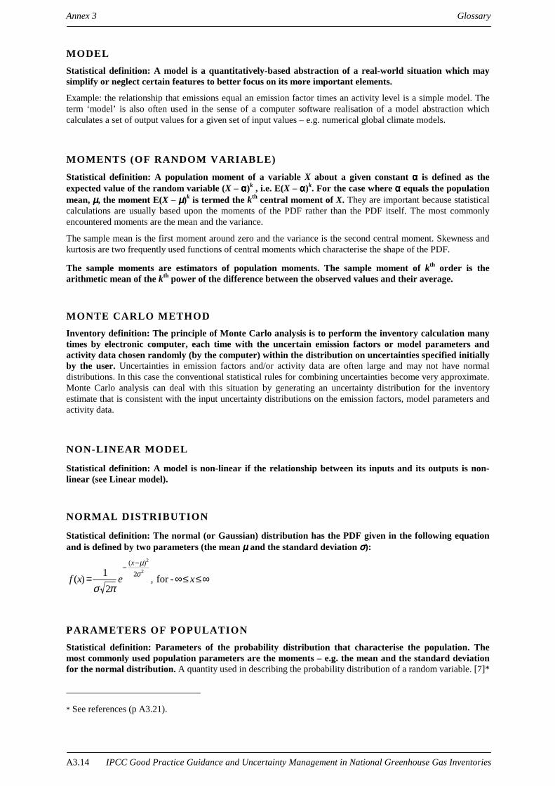
Annex 3 Glossary
IPCC Good Practice Guidance and Uncertainty Management in National Greenhouse Gas InventoriesA3.14
MODELStatistical definition: A model is a quantitatively-based abstraction of a real-world situation which maysimplify or neglect certain features to better focus on its more important elements.
Example: the relationship that emissions equal an emission factor times an activity level is a simple model. Theterm ‘model’ is also often used in the sense of a computer software realisation of a model abstraction whichcalculates a set of output values for a given set of input values – e.g. numerical global climate models.
MOMENTS (OF RANDOM VARIABLE)
Statistical definition: A population moment of a variable X about a given constant αααα is defined as theexpected value of the random variable (X – αααα)k , i.e. E(X – αααα)k. For the case where αααα equals the populationmean, µµµµ, the moment E(X – µµµµ)k is termed the kth central moment of X. They are important because statisticalcalculations are usually based upon the moments of the PDF rather than the PDF itself. The most commonlyencountered moments are the mean and the variance.
The sample mean is the first moment around zero and the variance is the second central moment. Skewness andkurtosis are two frequently used functions of central moments which characterise the shape of the PDF.
The sample moments are estimators of population moments. The sample moment of kth order is thearithmetic mean of the kth power of the difference between the observed values and their average.
MONTE CARLO METHODInventory definition: The principle of Monte Carlo analysis is to perform the inventory calculation manytimes by electronic computer, each time with the uncertain emission factors or model parameters andactivity data chosen randomly (by the computer) within the distribution on uncertainties specified initiallyby the user. Uncertainties in emission factors and/or activity data are often large and may not have normaldistributions. In this case the conventional statistical rules for combining uncertainties become very approximate.Monte Carlo analysis can deal with this situation by generating an uncertainty distribution for the inventoryestimate that is consistent with the input uncertainty distributions on the emission factors, model parameters andactivity data.
NON-LINEAR MODEL
Statistical definition: A model is non-linear if the relationship between its inputs and its outputs is non-linear (see Linear model).
NORMAL DISTRIBUTION
Statistical definition: The normal (or Gaussian) distribution has the PDF given in the following equationand is defined by two parameters (the mean µµµµ and the standard deviation σσσσ):
∞≤≤∞=
−−
xexf
x
-for ,2
1)(2
2
2) (
σµ
πσ
PARAMETERS OF POPULATIONStatistical definition: Parameters of the probability distribution that characterise the population. Themost commonly used population parameters are the moments – e.g. the mean and the standard deviationfor the normal distribution. A quantity used in describing the probability distribution of a random variable. [7]*
* See references (p A3.21).

Annex 3 Glossary
IPCC Good Practice Guidance and Uncertainty Management in National Greenhouse Gas Inventories A3.15
See Probability density function.
PERCENTILE
Statistical definition: The kth percentile or population percentile is a value which separates the lowest kth
part of the integral of the PDF – i.e. an integral of a PDF tail from the kth percentile towards lowerprobability densities.The kth population percentile (0 ≤ k ≤ 100) of a population with a distribution function F(x) equals to z where zsatisfies F(z) = k/100
Sample kth percentile is an approximation for the population percentile which is derived from a sample. Itis the value below which k percent of the observations lie.
POPULATION
Statistical definition: The population is the totality of items under consideration. In the case of a randomvariable, the probability distribution is considered to define the population of that variable [7]*.
Example: all conceivable experiments or events of a given type.
PRECISION
Inventory definition: Precision is the inverse of uncertainty in the sense that the more precise something is,the less uncertain it is.
PROBABILITYStatistical definition: A probability is a real number in the scale 0 to 1 attached to a random event. ([7]*,C.2.1) There are different ways in which probability can be interpreted. One interpretation considers aprobability as having the nature of a relative frequency (i.e. the proportion of all outcomes corresponding to anevent), whilst another interpretation regards a probability as being a measure of degree of belief. The probabilitythat a random event E occurs is often denoted as Pr(E). Probabilities may also be expressed in percentage terms.Probability theory is a branch of mathematics developed from axiomatic foundations, whose results underlaystatistical inference.
PROBABILITY DENSITY FUNCTION – PDFStatistical definition: A probability density function (PDF) is a mathematical function which characterisesthe probability behaviour of population. It is a function f(x) which specifies the relative likelihood of acontinuous random variable X taking a value near x, and is defined as the probability that X takes a value betweenx and x+dx, divided by dx where dx is an infinitesimally small number. Most PDFs require one or moreparameters to specify them fully.
The probability that a continuous random variable X lies in between the values a and b is given by the interval ofthe PDF, f(x), over the range between a and b.
∫=<≤a
b
dxxfbxa )()Pr(
The PDF is the derivative (when it exists) of the distribution function:
* See references (p A3.21).

Annex 3 Glossary
IPCC Good Practice Guidance and Uncertainty Management in National Greenhouse Gas InventoriesA3.16
f x dF xdx
( ) ( )=
In practical situations, the PDF used is chosen from a relatively small number of standard PDFs and the mainstatistical task is to estimate its parameters. Thus, for inventory applications, a knowledge of which PDF has beenused is a necessary item in the documentation of an uncertainty assessment.
PROBABILITY DISTRIBUTIONStatistical definition: A function giving the probability that a random variable takes any given value orbelongs to a given set of values. The probability on the whole set of values of the random variable equals 1.[7]*
PROPAGATION OF UNCERTAINTIES
Statistical definition: The rules for propagation of uncertainties specify how to algebraically combine thequantitative measures of uncertainty associated with the input values to the mathematical formulae usedin inventory compilation, so as to obtain corresponding measures of uncertainty for the output values. SeeChapter 6, Quantifying Uncertainties in Practice, and Annex 1, Conceptual Basis for UncertaintyAnalysis.
QUALITY ASSURANCE (QA)
Inventory definition: Quality Assurance (QA) activities include a planned system of review proceduresconducted by personnel not directly involved in the inventory compilation/development process to verifythat data quality objectives were met, ensure that the inventory represents the best possible estimate ofemissions and sinks given the current state of scientific knowledge and data available, and support theeffectiveness of the quality control (QC) programme.
QUALITY CONTROL (QC)Inventory definition: Quality Control (QC) is a system of routine technical activities, to measure andcontrol the quality of the inventory as it is being developed. The QC system is designed to:
(i) Provide routine and consistent checks to ensure data integrity, correctness, andcompleteness;
(ii) Identify and address errors and omissions;
(iii) Document and archive inventory material and record all QC activities.
QC activities include general methods such as accuracy checks on data acquisition and calculations andthe use of approved standardised procedures for emission calculations, measurements, estimatinguncertainties, archiving information and reporting. Higher tier QC activities include technical reviews ofsource categories, activity and emission factor data, and methods.
RANDOM ERROR
See Systematic and random errors.
RANDOM VARIABLE
Statistical definition: A variable that may take any of the values of a specified set of values and with which
* See references (p A3.21).

Annex 3 Glossary
IPCC Good Practice Guidance and Uncertainty Management in National Greenhouse Gas Inventories A3.17
is associated a probability distribution. A random variable which may take only isolated values is said tobe ‘discrete.’ A random variable that may take any value within a finite or infinite interval is said to be‘continuous’. [7]*
RESIDUALStatistical meaning: For an observed value whose behaviour is modelled by a statistical model, theresidual is the difference between the observed value and the value predicted by the model, e.g. by linearregression. The residual is thus the component of an observation that cannot be explained by the model.
SAMPLE
Statistical meaning: A sample is a finite set of observations drawn from a population.
SENSITIVITYStatistical definition: A sensitivity is a measurement of how responsive one quantity is to a change inanother related quantity. The sensitivity of a quantity Y that is affected by changes in another quantity X, isdefined as the change in Y divided by the change in X that caused the changes in Y.
SENSITIVITY ANALYSISStatistical definition: Sensitivity analysis is a study of a model algorithm to determine how sensitive (orstable) it is to variations of its input data or underlying assumptions. It is performed by varying input valuesor model equations and observing how the model output varies correspondingly. The aim of such a sensitivityanalysis can include:
• observing the range of output values corresponding to input variables lying within ‘reasonable’ ranges; and
• calculating finite difference approximations for elasticities and sensitivities as required by somemethodologies for studying error propagation within a system.
SIGMA INTERVAL
Statistical definition: A c-sigma interval is a symmetric confidence interval centred on the mean andextending c times the standard deviation on either side.
SIMPLE RANDOM SAMPLE
Statistical definition: A sample of n items chosen from a population such that every possible sample hasthe same probability of being chosen.
SKEWNESSStatistical definition: Skewness is a measure of asymmetry of a PDF. It is a simple function of two
moments of the PDF, given by: 33
232
3
σµ
µµ
γ == where µ2, µ3, and σ, are central moments. Symmetric
distributions have γ = 0. The same name is frequently used for sample skewness, in which case both populationmoments are replaced by sample moments.
* See references (p A3.21).

Annex 3 Glossary
IPCC Good Practice Guidance and Uncertainty Management in National Greenhouse Gas InventoriesA3.18
STANDARD DEVIATIONStatistical definition: The population standard deviation is the positive square root of the variance. It isestimated by the sample standard deviation that is the positive square root of the sample variance.
STANDARD ERROR OF THE MEANStatistical definition: A term often used to signify the sample standard deviation of the mean.
STATISTIC
Statistical definition: A statistic is a function of the sample random variables. [7]*
STATISTICS
Statistical definition: Statistics can refer either in a general sense to the compilation of data, frequentlyabout human activities, or in a more specific sense to the branch of science concerned with the systematicnumerical treatment of data derived from aggregates of items.
SYSTEMATIC AND RANDOM ERRORS
Statistical definition: Systematic error is the difference between the true, but usually unknown, value of aquantity being measured, and the mean observed value as would be estimated by the sample mean of aninfinite set of observations. The random error of an individual measurement is the difference between anindividual measurement and the above limiting value of the sample mean.
SYSTEMATIC ERROR
Statistical definition: See Systematic and random errors.
TIME SERIES
Statistical definition: A time series is series of values which are affected by random processes and whichare observed at successive (but usually equidistant) time points.
TRANSPARENCYInventory definition: Transparency means that the assumptions and methodologies used for an inventoryshould be clearly explained to facilitate replication and assessment of the inventory by users of thereported information. The transparency of inventories is fundamental to the success of the process for thecommunication and consideration of information.
TRENDInventory definition: The trend of a quantity measures its relative trend over a time period, with a positivetrend value indicating growth in the quantity, and a negative value indicating a decrease. It is defined asthe ratio of the change in the quantity over the time period, divided by the initial value of the quantity,and is usually expressed either as a percentage or a fraction.
* See references (p A3.21).

Annex 3 Glossary
IPCC Good Practice Guidance and Uncertainty Management in National Greenhouse Gas Inventories A3.19
TRIANGULAR DISTRIBUTION
Statistical definition: An asymmetric triangular distribution function has a PDF
f(x) = 2(x – a) / {(b – a) (m – a)} when a ≤≤≤≤ x ≤≤≤≤ m and a < m ≤≤≤≤ b
= 2(b – x) / {(b – a) (b – m)} when m ≤≤≤≤ x ≤≤≤≤ b and a ≤≤≤≤ m < b
= 0 elsewhere,
where the parameters which specify the distribution are the minimum value a, the maximum value b, andthe most likely position (i.e. mode) m, subject to a ≤≤≤≤ m ≤≤≤≤ b.
UNBIASED ESTIMATORStatistical definition: An unbiased estimator is a statistic whose expected value equals the value of theparameter being estimated. Note that this term has a specific statistical meaning and that an estimate of aquantity calculated from an unbiased estimator may lack bias in the statistical sense, but may be biased in themore general sense of the word if the sample has been affected by unknown systematic error. Thus, in statisticalusage, a biased estimator can be understood as a deficiency in the statistical evaluation of the collected data, andnot in the data themselves or in the method of their measurement or collection. For example, the arithmetic mean(average) x is an unbiased estimator of the expected value (mean).
UNCERTAINTYStatistical definition: An uncertainty is a parameter, associated with the result of measurement thatcharacterises the dispersion of the values that could be reasonably attributed to the measured quantity.[7]* (e.g. the sample variance or coefficient of variation)
Inventory definition: A general and imprecise term which refers to the lack of certainty (in inventorycomponents) resulting from any causal factor such as unidentified sources and sinks, lack of transparency etc.
UNCERTAINTY ANALYSIS
Statistical definition: An uncertainty analysis of a model aims to provide quantitative measures of theuncertainty of output values caused by uncertainties in the model itself and in its input values, and toexamine the relative importance of these factors.
UNIFORM DISTRIBUTION
Statistical definition: A random variable with a uniform or rectangular distribution is confined to liewithin a range over which all values are equally probable. If the upper and lower limits of the range are aand b respectively, the PDF is a flat function from a to b (the two parameters defining the PDF).The PDF of a uniform distribution is given by:
≤≤
−=elsewhere0
for1)( bxa
abxf
where
2ba +
=µ
is the mean and
* See references (p A3.21).
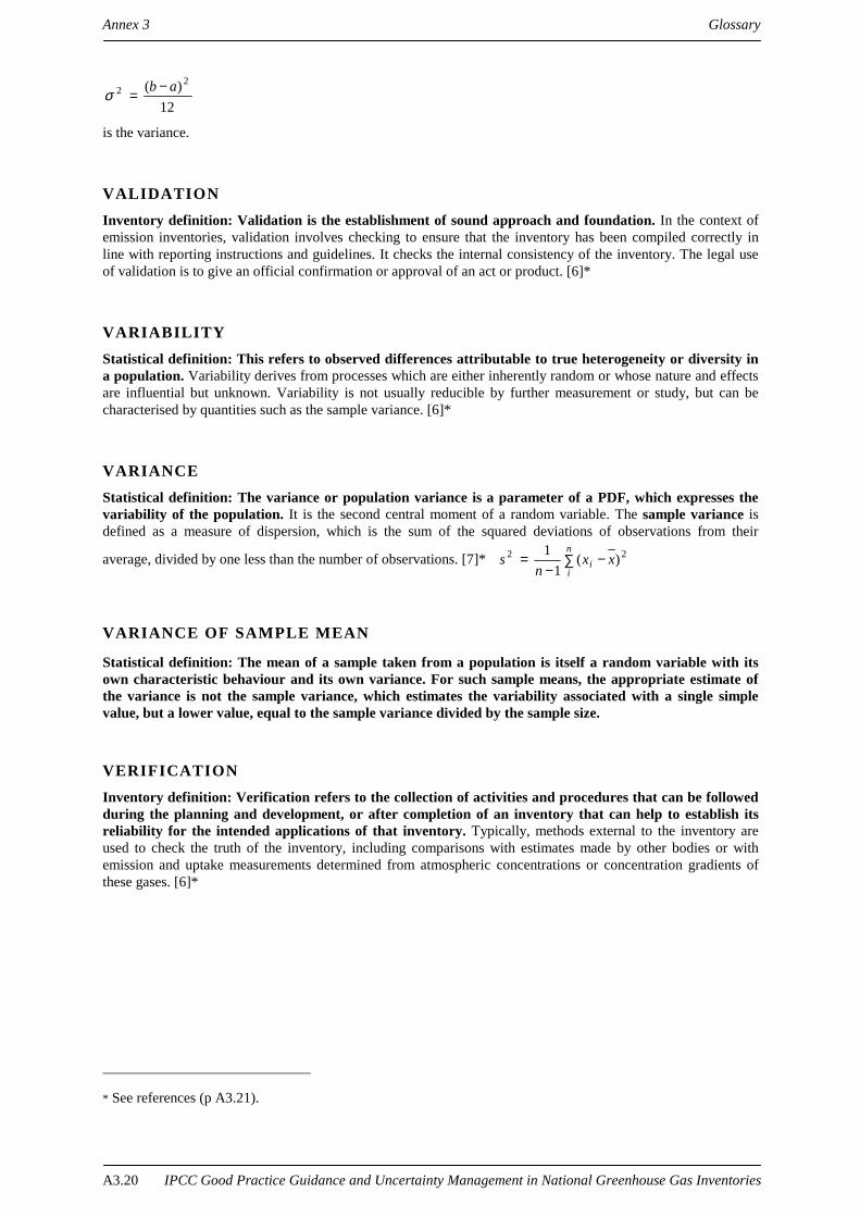
Annex 3 Glossary
IPCC Good Practice Guidance and Uncertainty Management in National Greenhouse Gas InventoriesA3.20
12)( 2
2 ab −=σ
is the variance.
VALIDATIONInventory definition: Validation is the establishment of sound approach and foundation. In the context ofemission inventories, validation involves checking to ensure that the inventory has been compiled correctly inline with reporting instructions and guidelines. It checks the internal consistency of the inventory. The legal useof validation is to give an official confirmation or approval of an act or product. [6]*
VARIABILITYStatistical definition: This refers to observed differences attributable to true heterogeneity or diversity ina population. Variability derives from processes which are either inherently random or whose nature and effectsare influential but unknown. Variability is not usually reducible by further measurement or study, but can becharacterised by quantities such as the sample variance. [6]*
VARIANCEStatistical definition: The variance or population variance is a parameter of a PDF, which expresses thevariability of the population. It is the second central moment of a random variable. The sample variance isdefined as a measure of dispersion, which is the sum of the squared deviations of observations from their
average, divided by one less than the number of observations. [7]* ∑ −−
=n
ii xx
ns 22 )(
11
VARIANCE OF SAMPLE MEAN
Statistical definition: The mean of a sample taken from a population is itself a random variable with itsown characteristic behaviour and its own variance. For such sample means, the appropriate estimate ofthe variance is not the sample variance, which estimates the variability associated with a single simplevalue, but a lower value, equal to the sample variance divided by the sample size.
VERIFICATIONInventory definition: Verification refers to the collection of activities and procedures that can be followedduring the planning and development, or after completion of an inventory that can help to establish itsreliability for the intended applications of that inventory. Typically, methods external to the inventory areused to check the truth of the inventory, including comparisons with estimates made by other bodies or withemission and uptake measurements determined from atmospheric concentrations or concentration gradients ofthese gases. [6]*
* See references (p A3.21).

Annex 3 Glossary
IPCC Good Practice Guidance and Uncertainty Management in National Greenhouse Gas Inventories A3.21
REFERENCES[1] Brandt S. (1970). Computational Methods in Statistics and Data Analysis. North-Holland, Amsterdam,
Netherlands.
[2] Wonnacott R. and Wonnacott T. (1990). Introductory Statistics for Business and Economics. John Wiley,New York, USA.
[3] Zijp W.L. (1987). Treatment of measurement of Uncertainties. ECN-194, Petten, Netherlands.
[4] Martin B.R. (1971). Statistics for Physicists. Academic Press, London, UK.
[5] Kendall M. G, Stuart A. (1966). The Advanced Theory of Statistics. Charles Grifiin & Co.Ltd, London, UK.
[6] Intergovernmental Panel on Climate Change (IPCC) (1998). Meeting Report: Managing Uncertainty inNational Greenhouse Gas Inventories, Report of the meeting held in Paris 13-15, October 1998,IPCC/OECD/IEA Programme on National Greenhouse Gas Inventories.
[7] International Organization for Standardization (ISO) (1993). Guide to the expression of uncertainty inmeasurement. ISBN 92-67-10188-9, ISO, Geneva, Switzerland.
[8] Kotz, S. and Johnson, N.L. (1988). Encyclopaedia of Statistical Sciences. 9 volumes, John Wiley & Sons,New York, USA.
[9] Intergovernmental Panel on Climate Change (IPCC) (1997). Revised 1996 IPCC Guidelines for NationalGreenhouse Gas Inventories: Volume 1 Reporting Instructions. J.T. Houghton et al., IPCC/OECD/IEA,Paris, France.

Annex 4 List of Participants
IPCC Good Practice Guidance and Uncertainty Management in National Greenhouse Gas Inventories A4.1
A N N E X 4
LIST OF PARTICIPANTS
List of Participants Annex 4
IPCC Good Practice Guidance and Uncertainty Management in National Greenhouse Gas InventoriesA4.2
PARTICIPANT INSTITUTION COUNTY MEETING
ABEL, Kay Australian Greenhouse Office Australia IndustrialProcesses
AgricultureUncertaintyFinalisation
ABUBAKAR, Osman Sudan Meteorlogical Authority Sudan Uncertainty
ADAMKOVA, Juliana Slovak Hydrometeorological Institute Slovak Republic Waste
AGARWAL, Radhy .S. Mechanical Engineering Department, India IndustrialIndian Institute of Technology Delhi Processes
AGUIAR PEIXOTO, Department of Mechanical Engineering, Brazil IndustrialRoberto de Instituto Mauá De Tecnologia Processes
AGYEMANG-BONSU, Environmental Protection Agency Ghana IndustrialWilliam Processes
Uncertainty
AITCHISON, Kenneth Novellus Systems, Inc. USA IndustrialProcesses
ALVES, Joao W. da Silva CETESB Brazil Waste
AMON, Barbara Institute of Agricultural, Austria AgricultureEnvironmental, and Energy Engineering,University of Agricultural Sciences
AMOUS, Samir Apex-EBBD Consulting Co Tunisia Energy
ARMSTRONG-BROWN, UK Ministry of Agriculture, Fisheries, UK AgricultureSue and Food
ASHFORD, Paul Caleb Management Services UK Industrial Processes
ATKINSON, Mike Diamantina Technology Australia IndustrialProcesses
Finalisation
ATKINSON, Ward Sun Test Engineering USA Industrial Processes
BAKER, James A. Delphi Automotive Systems USA Industrial Processes
BAKSHI, Vikram ICF, Inc. USA Industrial Processes
BALDASANO, Jose Dpto. de Proyectos de Ingenieria, Spain WasteUniversidad Politecnica de Cataluna Finalisation
BARBOUR, Wiley Office of Policy, Planning & Evaluation, USA IndustrialUS Environmental Protection Agency, ProcessesClimate Change Division Energy
UncertaintyFinalisation
BARRY, Simon Bureau of Rural Sciences Australia Finalisation
BARTOS, Scott US Environmental Protection Agency USA Industrial Processes
BEEVER, David CEDAR, Dept. of Agriculture, UK AgricultureThe University of Reading
BENTLEY, Simon CSIRO Atmospheric Research Australia UncertaintyFinalisation
BERRA, Guillerm Instituto de Patobiologia Argentina Agriculture

Annex 4 List of Participants
IPCC Good Practice Guidance and Uncertainty Management in National Greenhouse Gas Inventories A4.3
BEU, Laurie Motorola USA Industrial Processes
BHIDE, A. D. National Environmental Engineering India WasteResearch Institute
BIGG, Martin Environment Agency UK Waste
BITSCH, Rainer Siemens AG EV DE Germany Industrial Processes
BJERKE, Willy International Primary Aluminium Institute UK Industrial Processes
BOECKX, Pascal University of Ghent Belgium WasteFinalisation
BOGDANOV, Stanislav National Institute of Meteorology, Bulgaria Industrialand Hydrology Processes
BOILEAU, Pierre Environment Canada Canada IndustrialProcesses
BOUCHARD, Guy Alcan International Limitée, Canada IndustrialCentre de recherche et de Processesdéveloppement Arvida
BOUWMAN, A.F. National Institute of Public Health Netherlands Agricultureand the Environment (RIVM)
BRAATZ, Barbara ICF Consulting Group USA Agriculture
BRANSCOME, Marvin Research Triangle Institute USA IndustrialProcesses
BREED, William US Department of Energy USA Uncertainty
BRENNAN, Jean Office of Global Change, USA AgricultureUS Department of State Energy
BROTHERS, Lowell Southern Company Services USA IndustrialProcesses
BROWN, Keith AEA Technology Environment UK Waste
BUJIDMAE, B Institute of Meteorology and Mongolia AgricultureHydrology
BURTON, C. Shepherd ICF Kaiser Consulting Group, USA IndustrialSystems Applications International, Inc. Processes
CAHYONO ADI, Agus Agency for Assessment and Application Indonesia Energyof Technology (BPP Technology) Finalisation
CAMPBELL, Nick ICI Klea UK IndustrialProcesses
CARRUTHERS, Ian Australian Greenhouse Office Australia Finalisation
CICERO, Anita International Pharmaceutical Aerosol USA IndustrialConsortium (IPAC) Processes
CHANG, Jean-Pierre CITEPA France UncertaintyFinalisation
CHRISTMAS, Mark DuPont Fluoroproducts USA IndustrialProcesses
CLARKE, Rachael Australian Greenhouse Office Australia Finalisation
CLODIC, Denis Ecole des Mines de Paris France IndustrialProcesses
DARRAS, Marc Gaz de France France Energy

List of Participants Annex 4
IPCC Good Practice Guidance and Uncertainty Management in National Greenhouse Gas InventoriesA4.4
DE LAURETIS, Riccardo Environmental Protection Agency (ANPA) Italy UncertaintyFinalisation
DENIER VAN DER GON, Lab of Soil Science and Geology, Netherlands AgricultureHugo Wageningen Agricultural University
DOLIN, Eric US Environmental Protection Agency USA IndustrialProcesses
DOMINGOS MIGUEZ, José Ministry of Science and Technology Brazil Energy
DONG, Hongmin Chinese Academy of Agricultural Sciences China Agriculture
DOORN, Michiel ARCADIS Geraghty & Miller Netherlands WasteFinalisation
DU TOIT, Pieter SASTECH Research and Development South Africa IndustrialProcesses
Finalisation
EGGLESTON, Simon AEA Technology, National Environmental UK EnergyTechnology Centre (NETCEN) Uncertainty
Finalisation
ELLERTON, Kathryn Allied Signal, Inc. USA Industrial Processes
El-MOWAFY, Smair Attia Egyptian Environmental Affairs Agency Egypt Energy
ESALA, Martti Plant Production Research, Finland AgricultureCrops and Soil, Agricultural Research Centre
FALK, Robert S. Department of Trade and Industry UK Energy
FAY, Kevin International Climate Change Partnership USA IndustrialProcesses
FERNÁNDEZ, The National Commission for the Chile UncertaintyMarcelo Rodrigo Environment,
Metropolitan Region Department,Air Decontamination Area
FONTELLE, Jean-Pierre CITEPA France EnergyUncertaintyFinalisation
FORTE, Reynaldo US Environmental Protection Agency USA IndustrialProcesses
Finalisation
FOTT, Pavel Czech Hydrometeorological Institute Czech Republic EnergyUncertaintyFinalisation
FREY, Christopher Dept. of Civil Engineering, USA UncertaintyNorth Carolina State University
FUJIMOTO, Yuichi Japan Industrial Conference for Japan IndustrialOzone Layer Protection Processes
GALBALLY, Ian CSIRO Atmospheric Research Australia AgricultureUncertaintyFinalisation
GASCA, Jorge Mexican Petroleum Institute Mexico UncertaintyFinalisation
GERBENS, Sybren Department of Manure and Agricultural Netherlands AgricultureByproducts, Institute of Agricultural andEnvironmental Engineeering
GERMON, Jean-Claude INRA France Agriculture
Annex 4 List of Participants
IPCC Good Practice Guidance and Uncertainty Management in National Greenhouse Gas Inventories A4.5
GIBBS, Michael ICF Consulting Group USA IndustrialProcesses
AgricultureFinalisation
GILLENWATER, Michael US Environmental Protection Agency USA IndustrialProcesses
EnergyUncertaintyFinalisation
GILLET, Marc Mission Interministérielle de l’Effet de Serre France Finalisation
GJERALD, Eilev Norwegian Pollution Control Authority Norway Energy(SFT) Uncertainty
Finalisation
GNAPELET, Lambert Ministry of Environment, Water, Forest, Central African RepublicHunting, and Fisheries Agriculture
GOMEZ, Dario Comision Nacional de Energia Atomica, Argentina EnergyUnidad de Actividad Quimica
GREEN, David National Institute of Standards and USA IndustrialTechnology Processes
GREENE, Dave Oak Ridge National Laboratory (ORNL) USA Energy
GROENESTEIN, Karin Institue of Agricultural and Environmental Netherlands AgricultureEngineering (IMAG-DLO)
GRONFORS, Kari Statistics Finland Finland EnergyUncertaintyFinalisation
GRUNCHARD, Francis Solvay Belgium IndustrialProcesses
GYTARSKY, Michael Institute of Global Climate and Ecology Russia AgricultureUncertaintyFinalisation
HABTETSION, Semere Department of Energy Eritrea Uncertainty
HANNA, Javier Programa Nacional de Cambios Bolivia EnergyClimaticos Finalisation
HAO, Wei Min USDA Forest Service USA Agriculture
HARNISCH, Jochen ECOFYS Energy and Environment Germany IndustrialProcesses
Agriculture
HARPER, Lowry US Department of Agriculture USA Agriculture
HEINEMEYER, Otto FAL/BML Germany Agriculture
HENRY, Beverley Queensland Department of Natural Resources Australia Finalisation
HEROLD, Anke Oeko-Institut Germany EnergyWasteUncertaintyFinalisation
HIRAISHI, Taka National Institute for Environmental Studies Japan Industrial(NIES), Environment Agency Processes
EnergyWasteUncertaintyFinalisation

List of Participants Annex 4
IPCC Good Practice Guidance and Uncertainty Management in National Greenhouse Gas InventoriesA4.6
HIRATA, Toshio Denso Corporation Japan IndustrialProcesses
HOBSON, John Water Research Centre UK Waste
HOSSAIN, Ijaz Bangladesh University of Engineering and Bangladesh EnergyTechnology
IRPOLA, Eliisa Finnish Environment Institute Finland IndustrialProcesses
IRVING, William US Environmental Protection Agency USA IndustrialProcesses
AgricultureEnergyWasteUncertaintyFinalisation
JACOBS, Cindy Office of Mobile Sources, USA EnergyUS Environmental Protection Agency
JACOBS, Franck Morgen Statistics Division, Ministry of Planning Antigua Uncertainty
JACQUES, Art Environment Canada Canada UncertaintyFinalisation
JANSSEN, Leon National Institute of Public Health and the Netherlands AgricultureEnvironment (RIVM)
JARVIS, Stephen Institute of Grassland and Environmental UK AgricultureResearch
JEFFS, Mike ICI Polyurethanes Belgium IndustrialProcesses
JENSEN, Jens F. Frøiland Norconsult Norway Waste
JOHNSON, Don Colorado State University USA Agriculture
JUBB, Charles Burnbank Consulting Pty.Ltd. Australia WasteUncertainty
JUN, Paul ICF Consulting Group USA Agriculture
KELLER, Fred Carrier Corporation USA IndustrialProcesses
KERR, Thomas SCS Engineers USA Waste
KILDE, Niels RISOE National Laboratory Denmark Agriculture
KIPONDYA, Wilfred Centre for Energy, Environment, Tanzania EnergyScience and Technology
KLEFFELGAARD, Tore Norwegian Pollution Control Authority (SFT) Norway Waste
KOCH, Dietmar Federal Environmental Agency Germany Energy
KOCH, Jean SOREQ Nuclear Research Center Israel AgricultureFinalisation
KOHV, Natalja Estonian Environment Information Centre Estonia Uncertainty
KOKORIN, Alexey Institute of Global Climate and Ecology Russia IndustrialProcesses
Finalisation
KRANJC, Andrej Hydrometeorological Institute of Slovenia Slovenia Waste
KROEZE, Carolien Wageningen Institute for Environment and Netherlands AgricultureClimate Research (WIME),Wageningen Agricultural University

Annex 4 List of Participants
IPCC Good Practice Guidance and Uncertainty Management in National Greenhouse Gas Inventories A4.7
KRUGER, Dina US Environmental Protection Agency USA IndustrialProcesses
AgricultureEnergyWasteUncertaintyFinalisation
KUNWAR, Purushottam Ministry of Population and Environment Nepal IndustrialProcesses
KUTAS, Jozef IEM's Institute for Environmental Protection Hungary Waste
KWASI ADU, Joseph Animal Research Instittute Ghana AgricultureFinalisation
LAMOTTA, Sergio ENEA Italy Energy
LANTIN, Rhoda International Rice Research Institute Philippines Agriculture
LARA, Scarlette INIA-La Platina, Chile WasteInstituto de Investigaciones Agropecuarias
LASSEY, Keith National Institute of Water and Atmospheric New Zealand AgricultureResearch (NIWA) Finalisation
LEBER, Bernard Kaiser Aluminum USA IndustrialProcesses
LEVAVASSEUR, Philippe SGS-Thompson Microelectronics France IndustrialProcesses
LIEBERMAN, Elliot US Environmental Protection Agency USA Energy
LINDH, Nils Swedish Environmental Protection Agency Sweden Uncertainty
LOPEZ, Carlos Instituto de Meteorologia Cuba Finalisation
LOTT, Robert Gas Research Institute USA Energy
LUCON, Oswaldo CETESB Brazil Waste
LYCK, Erik National Environmental Research Institute Denmark Agriculture
MAGEZI-AKIIKI, B. James Department of Meteorology Uganda Uncertainty
MAHRENHOLZ, Petra Federal Environmental Agency Germany IndustrialProcesses
MAINHARDT, Heike ICF, Inc. USA IndustrialProcesses
MANGINO, Joe Eastern Research Group USA IndustrialProcesses
UncertaintyFinalisation
MARECKOVA, Katarina Slovak Hydrometeorological Institute, Slovak Republic IndustrialDepartment of Environment Processes
AgricultureEnergyWasteUncertaintyFinalisation
MARKS, Jerry ALCOA USA IndustrialProcesses
MARTINEZ, Julia Instituto Nacional de Ecologia/SENARNAP Mexico IndustrialProcesses
MATSUO, Naoki Institute for Global Environmental Strategies Japan Uncertainty(IGES)

List of Participants Annex 4
IPCC Good Practice Guidance and Uncertainty Management in National Greenhouse Gas InventoriesA4.8
MAUSCHITZ, Gerd Vienna University of Technology Austria Waste
MCCULLOCH, Archie ICI Chemicals and Polymers, Ltd. UK Industrial Processes Finalisation
McFARLAND, Mack DuPont Fluoroproducts USA IndustrialProcesses
McNAMARA, Pauline Swiss Agency for the Environment, Forest Switzerland Uncertaintyand Landscape
MEYER, Leo Department of Climate Change Netherlands FinalisationMinistry of Housing, Physical Planning,and the Environment
MIDAGLIA, Carmen CETESB Brazil Waste
MIGUEZ, José Domingos Ministry of Science and Technology Brazil Finalisation
MILTON, Martin National Physical Laboratory UK Waste
MIROSLAV, Markvart Institute of Inorganic Chemistry, Czech Republic EnergyCzech Academy of Sciences
MOCELLA, Michael DuPont Fluoroproducts USA IndustrialProcesses
MOHAMED, Yahaiya Ministère de l'Environnement Comores Agriculture
MONDSHINE, Michael Science Applications International Corporation USA Waste (SAIC)
MOSIER, Arvin U.S.Department of Agriculture USA AgricultureAgricultural Research Service (USDA/ARS) Finalisation
MUPETA, Bart Henderson Research Station Zimbabwe Agriculture
MYERS, Jerry Intel Corporation USA IndustrialProcesses
NAKHUTIN, Alexander Institute of Global Climate and Ecology Russia UncertaintyFinalisation
NAUJOCK, Art Calsonic North America USA IndustrialProcesses
NEITZERT, Frank Environment Canada Canada EnergyUncertaintyFinalisation
NEVISON, Cindy National Center for Atmospheric Research USA Agriculture(NCAR)
NGARA, Todd Climate Change Office, Zimbabwe UncertaintyMinistry of Mines and Environment
NYENZI, Buruhani Drought Monitoring Centre (DMC) Tanzania EnergyWasteUncertaintyFinalisation
OBATA, Yutaka Calsonic Corporation Japan IndustrialProcesses
ODINGO, Richard University of Nairobi Kenya UncertaintyFinalisation
OENEMA, Oene AB-DLO Netherlands Agriculture Finalisation

Annex 4 List of Participants
IPCC Good Practice Guidance and Uncertainty Management in National Greenhouse Gas Inventories A4.9
OGHITA, Toshiaki Institute for Techno-Economics Japan IndustrialProcesses
Finalisation
OI, Michihiro Environment Agency Japan Energy
OLIVIER, Jos National Institute of Public Health and the Netherlands IndustrialEnvironment (RIVM) Processes Uncertainty Finalisation
OLSEN, Kenneth Environment Canada Canada AgricultureWaste
OLSSON, Astrid Swedish Environmental Protection Agency Sweden IndustrialProcesses
Energy
OONK, Hans TNO-MEP Netherlands Waste
OSMAN, Nejib National Agency of Renewable Energy Tunisia Energy
OTTINGER SCHAEFER, US Environmental Protection Agency USA IndustrialDeborah Processes
OWENS, John 3M Chemicals USA IndustrialProcesses
PACIORNIK, Newton Ministry of Science and Technology, Brazil IndustrialFurnas Centrais Eletricas Processes
EnergyWasteUncertaintyFinalisation
PALMER, Bill Cheminfo Services, Inc. Canada IndustrialProcesses
PARADIZ, Bostjan Hydrometeorological Institute of Slovenia Slovenia WasteUncertaintyFinalisation
PARASYUK, Natalya Agency for Rational Energy Use and Ecology Ukraine IndustrialProcesses
PENMAN, Jim Global Atmosphere Division UK IndustrialDepartment of the Environment, Transport Processesand the Regions Agriculture
EnergyWasteUncertaintyFinalisation
PETITJEAN, Christophe Valeo Thermique Habitacle France IndustrialProcesses
PETTERSEN, Marit Viktoria Norwegian Pollution Control Authority Norway IndustrialProcesses
PHILLIPS, Marc Enron Gas Pipeline Group USA Energy
PICARD, David Clearstone Engineering, Ltd. Canada EnergyFinalisation
PIPATTI, Riitta VTT Energy Finland AgricultureWasteUncertaintyFinalisation
PREISEGGER, Ewald Solvay Germany IndustrialProcesses

List of Participants Annex 4
IPCC Good Practice Guidance and Uncertainty Management in National Greenhouse Gas InventoriesA4.10
PRETEL, Jan Czech Hydrometeorological Institute Czech Republic EnergyFinalisation
PULLEN, John Alcoa of Australia, Ltd. Australia IndustrialProcesses
PULLES, Tinus Institute of Environmental Sciences, Energy Netherlands EnergyResearch and Process Innovation TNO-MEP Uncertainty
Finalisation
RAJARATHNAM, Uma Tata Energy Research Institute (TERI) India Energy
RAMOS-MANE, Cecilia Uruguay Agriculture
RAND, Sally US Environmental Protection Agency USA IndustrialProcesses
RASMUSSEN, Erik Danish Energy Agency Denmark IndustrialProcesses
AgricultureEnergy
RECHBAUER, Gabriele GTZ Deutsche Gesellschaft fûr Technische, Germany IndustrialZusammenarbeit GmbH, Proklima/Measures Processes
REUCK, Karin INIA-La Platina, Instituto de Investigaciones Chile WasteAgropecuarias
REYENGA, Penny Australian Greenhouse Office Australia Finalisation
RIBACKE, Sara Swedish Association of Local Authority Sweden Energy
RIVIERE, Emmanuel CITEPA France IndustrialProcesses
Uncertainty
RODE, Bojan Hydrometeorological Insitutute of Slovenia Slovenia EnergyUncertaintyFinalisation
ROMANO, Daniela Environmental Protection Agency (ANPA) Italy UncertaintyFinalisation
ROSLAND, Audun Norwegian Pollution Control Authority Norway Finalisation
RUIZ-SUAREZ, Centro de Ciencias de la Atmosfera (UNAM) Mexico AgricultureLuis Gerardo
RUYSSENAARS, Paul Ministry of Housing, Spatial Planning and the Netherlands AgricultureEnvironment, Air and Energy
RYPDAL, Kristin Statistics Norway Norway IndustrialProcesses
AgricultureEnergyUncertaintyFinalisation
RYPINSKI, Arthur Energy Information Administration, USA IndustrialUS Department of Energy Processes
EnergyUncertaintyFinalisation
SABURI, Masataka Ministry of International Trade and Industry Japan IndustrialProcesses
SALWAY, Geoff AEA Technology, National Environmental UK UncertaintyTechnology Centre (NETCEN)
SASS, Ronald L.. Dept. of Ecology and Evolutionary Biology, USA AgricultureRice University

Annex 4 List of Participants
IPCC Good Practice Guidance and Uncertainty Management in National Greenhouse Gas Inventories A4.11
SCHMID, Martin Institute of Environmental Protection and Switzerland AgricultureAgriculture
SEIDEL, Stephen US Environmental Protection Agency USA IndustrialProcesses
SENHAJI, Faouzi Groupe d'Etudes et de Recherches sur les Morocco WasteE.R. et l'Environnement (GERERE) Uncertainty
Finalisation
SHENGCHU, Huang China Coalbed Methane Clearinghouse China Energy
SIMMONS, Tim AVONLOG Limited UK Energy
SISKA, Bernard Slovak Agricultural University Slovak Republic Agriculture
SMITH, Jeffery USDA-ARS USA Agriculture
SMITH, Keith Institute of Ecology and Resource UK AgricultureManagement (IERM), University of Edinburgh Finalisation
SOUZA LOMBA NETO, TEIXEIRA, Egle Novaes Brazil IndustrialCandido Processes
SPAKMAN, Jan National Institute of Public Health and the Netherlands EnergyEnvironment (RIMV)
STECZKO, Katarzyna Oil and Gas Institute Poland Waste
STIRPE, Dave Alliance for Responsible Atmospheric Policy USA IndustrialProcesses
STROGIES, Michael Federal Environmental Agency Germany IndustrialProcesses
AgricultureUncertaintyFinalisation
SUBAK, Susan NRDC USA Uncertainty
SUIZU, Takuya Federation of Electric Power Companies Japan IndustrialProcesses
SULLIVAN, Rory Pacific Air and Environment Australia Finalisation
SVENSSON, Ingvar Swedish Environmental Protection Agency Sweden Waste
SWATKOWSKI, Len Appliance Research Consortium USA IndustrialProcesses
TAILAKOV, Oleg Russian Coalbed Methane Center Russia Energy
TAYLOR, Dwayne Denso USA IndustrialProcesses
TAYLOR, Gary Taylor/Wagner, Inc. Canada IndustrialProcesses
TEIXEIRA, Egle Novaes Fac. Engenharia Civil – UNICAMP Brazil Waste
TICHY, Milos SUJB Czech Republic IndustrialProcesses
EnergyUncertaintyFinalisation
TOWPRAYOON, Joint Graduate School of Energy and the Thailand WasteSirintornthep Enviornment
King Mongkut's University of Technology
TRIPP, Tom Magnesium Corporation of America USA IndustrialProcesses
TSARUKYAN, Martiros Ministry of Nature Protection Armenia Uncertainty

List of Participants Annex 4
IPCC Good Practice Guidance and Uncertainty Management in National Greenhouse Gas InventoriesA4.12
TSURUTA, Haruo National Institute of Agro-Environmental Japan AgricultureSciences Finalisation
TUHKANEN, Sami Technical Research Centre of Finland Finland Energy
VAN AARDENNE, John A. Wageningen Center for Environment and Netherlands AgricultureClimate Studies (CMKW)
VAN AMSTEL, Andre Wageningen Agricultural University/WIMEK Netherlands AgricultureUncertainty
VAN BRUMMELEN, ECOFYS Netherlands IndustrialMargreet Processes
VAN OSS, Hendrik U.S. Geological Survey USA IndustrialProcesses
VERHILLE, Maurice ELF - Atochem France IndustrialProcesses
VICHULATA, Pravee Department of Animal Science, Thailand AgricultureKasetsart University
VIERA, Sonia Manso CETESB Brazil Waste
WALSH, Mike Technical Consultant USA Energy
WANG, Minxing Institute of Atmospheric Physics China FinalisationChinese Academy of Science
WEI, Zhihong Tsinghua University China IndustrialProcesses
Finalisation
WERKEMA, Tom ELF Atochem USA IndustrialProcesses
WILLIAMS, David J. CSIRO Energy Technology Australia EnergyUrban and Industrial Air Quality Finalisation
WILLIAMSON, Matthew US Environmental Protection Agency USA IndustrialProcesses
WINIWARTER, Wilfried Austrian Research Centers Austria Uncertainty
WIRTH, Thomas US Environmental Protection Agency USA Agriculture Finalisation
YAGI, Kazuyuki Japan International Research Center for Japan AgricultureAgricultural Sciences (JIRCAS) Finalisation
YASUDA, Kenji Kanagawa Environmental Research Center Japan Finalisation
YELLEN, Duncan March Consulting Group UK IndustrialProcesses
YESSERKEPOVA, Irina Kazakh Research Institute of Environment Kazakhstan WasteMonitoring and Climate
ZEEMAN, Grietje Department of Environment Technology, Netherlands AgricultureWageningen Agricultural University
ZHANG, Jim Environmental and Occupational Health USA EnergySciences Institute
ZHENLIN, Chen Department of Forecasting Services China Industrialand Disaster Mitigation, ProcessesChina Meteorological Administration Uncertainty
Finalisation
ZHOU, Peter EEGC CONSULTANTS Pty Botswana Uncertainty
Annex 4 List of Participants
IPCC Good Practice Guidance and Uncertainty Management in National Greenhouse Gas Inventories A4.13
PARTICIPANTS FROM INTERNATIONAL ORGANISATIONS
PARTICIPANT INSTITUTION MEETING
ACOSTA MORENO, UNFCCC Secretariat EnergyRoberto Agriculture
UncertaintyFinalisation
BUENDIA, Leandro IPCC-NGGIP/TSU UncertaintyFinalisation
DOBBIE, Leonie IATA Energy
EMMANUEL, Sal IPCC-NGGIP/TSU EnergyWasteUncertaintyFinalisation
HOEHNE, Niklas UNFCCC Secretariat IndustrialProcesses
Uncertainty
HOPPAUS, Robert IPCC-NGGIP/TSU IndustrialProcesses
AgricultureEnergyWaste
UncertaintyFinalisation
MARTINSEN, Thomas OECD, Environment Directorate IndustrialProcesses
AgricultureEnergyWasteUncertaintyFinalisation
MEIJER, Jeroen IPCC-NGGIP/TSU EnergyUncertaintyFinalisation
MIWA, Kyoko IPCC-NGGIP/TSU WasteUncertaintyFinalisation
SUNDARARAMAN, IPCC IndustrialNarasimhan Processes
TANABE, Kiyoto IPCC-NGGIP/TSU IndustrialProcesses
AgricultureWasteUncertaintyFinalisation
TREANTON, Karen International Energy Agency (IEA) EnergyUncertaintyFinalisation
WILLEMS, Stephane OECD, Environment Directorate Energy
WOODFIELD, Mike UNECE-Task Force on Emission Inventory Uncertainty