Good Features to Track

Jianbo Shi and Carlo Tomasi1

December 1993

1This research was supported by the National Science Foundation under contract IRI-9201751.This PDF file was recreated from the original LaTeX file for technical report TR 93-1399,Cornell University. The only changes were this note and the conversion of all the figure .epsfiles to .pdf files for compatibility with more recent page renderers and printers.

Abstract

No feature-based vision system can work until good features can be identified and tracked fromframe to frame. Although tracking itself is by and large a solved problem, selecting features thatcan be tracked well and correspond to physical points in the world is still an open problem. Wepropose a feature selection criterion that is optimal by construction because is based on how thetracker works, as well as a feature monitoring method that can detect occlusions, disocclusions, andfeatures that do not correspond to points in the world. These methods are based on a new trackingalgorithm that extends previous Newton-Raphson style search methods to work under affine imagetransformations. We test performance with several simulations and experiments on real images.

Chapter 1

Introduction

Is feature tracking a solved problem? The extensive studies of image correlation [CL74], [CR76],[RGH80], [Woo83], [FP86], [TH86] and sum-of-squared-difference (SSD) methods [BYX82], [Ana89]show that all the basics are in place. When image displacements are small from one frame to thenext, a window can be tracked by optimizing some matching criterion [LK81], [Ana89] over allpossible small translations and, in more sophisticated systems, over all moderate linear imagedeformations [F8̈7], [FM91], [MO93]. Furthermore, feature windows can be selected by maximizingan interest criterion, or some measure of texturedness or cornerness in the first image. Favoritecriteria are a high standard deviation in the spatial intensity profile [Mor80], the presence of zerocrossings of the Laplacian of the image intensity [MPU79], and corners [KR80], [DN81]. Finally,even the size of the window to be tracked can be selected adaptively based on local variations ofimage intensity and inter-frame disparity [OK92].

Yet a nagging problem remains open. In fact, even a region of high interest or rich texturecontent can be poor. For instance, it can straddle a depth discontinuity or the boundary of areflection highlight. In either case, the window is not attached to a fixed point in the world,making that feature useless or more likely harmful to most structure-from-motion algorithms. Thisphenomenon occurs very often. Extreme but typical examples are trees and cars. In a tree, branchesat different depths and orientations create intersections in the image that would trigger any featuredetector and yet correspond to no physical point in the world. With a car, most features on thebody and windows are reflections that change their position on the surface as the car drives pastthe camera. Even in carefully engineered imaging situations, the problem of poor features is sopervasive that good features must often be picked by hand. Furthermore, even good features canbe occluded by nearer surfaces, and trackers often blissfully drift away from their original point inthe world when this occurs. No vision system based on feature tracking can be claimed to reallywork until these issues have been settled.

In this report we show how to monitor the quality of image features during tracking. Specifically,we investigate a measure of feature dissimilarity that quantifies how much the appearance of afeature changes between the first and the current frame. The idea is straightforward: dissimilarityis the feature’s rms residue between the first and the current frame, and when dissimilarity growstoo large the feature should be abandoned. However, in this report we make two main contributionsto this problem. First, we provide experimental evidence that pure translation is not an adequatemodel for image motion when measuring dissimilarity, but affine image changes, that is, linearwarping and translation, are adequate. Second, we propose a numerically sound and efficient way

1

of determining affine changes by a Newton-Raphson stile minimization procedure, much in the styleof what Lucas and Kanade [LK81] do for the pure translation model.

In addition to these two main contributions, we improve tracking in two more ways. First, wepropose a more principled way to select features than the more traditional “interest” or “cornerness”measures. Specifically, we show that feature windows with good texture properties can be definedby explicitly optimizing the tracker’s accuracy. In other words, the right features are exactly thosethat make the tracker work best. Second, we submit that two models of image motion are betterthan one. In fact, pure translation gives more stable and reliable results than affine changes whenthe inter-frame camera translation is small. On the other hand, affine changes are necessary tocompare distant frames as is done when determining dissimilarity.

In the next chapter, we introduce affine image changes and pure translation as our two modelsfor image motion. In chapter 3 we describe our method for the computation of affine image changes.Then, in chapters 4 and 5, we discuss our measure of texturedness and feature dissimilarity, whichare based on the definition of the tracking method given in chapter 3. We discuss simulations andexperiments on real sequences in chapters 6 and 7, and conclude in chapter 8.

2

Chapter 2

Two Models of Image Motion

In this chapter, we introduce two models of image motion: the more general affine motion is acombination of translation and linear deformation, and will be described first. The second model,pure translation, is the restriction of the general model to zero deformation.

As the camera moves, the patterns of image intensities change in a complex way. In general,any function of three variables I(x, y, t), where the space variables x, y and the time variable t arediscrete and suitably bounded, can represent an image sequence. However, images taken at neartime instants are usually strongly related to each other, because they refer to the same scene takenfrom only slightly different viewpoints.

We usually express this correlation by saying that there are patterns that move in an imagestream. Formally, this means that the function I(x, y, t) is not arbitrary, but satisfies the followingproperty:

I(x, y, t+ τ) = I(x− ξ(x, y, t, τ), y − η(x, y, t, τ)) . (2.1)

Thus, a later image taken at time t+τ can be obtained by moving every point in the current image,taken at time t, by a suitable amount. The amount of motion δ = (ξ, η) is called the displacementof the point at x = (x, y) between time instants t and t+ τ .

Even in a static environment under constant lighting, the property described by equation (2.1)is often violated. For instance, at occluding boundaries, points do not just move within the image,but appear and disappear. Furthermore, the photometric appearance of a surface changes whenreflectivity is a function of the viewpoint. However, the invariant (2.1) is by and large satisfied atsurface markings that are away from occluding contours. At these locations, the image intensitychanges fast with x and y, and the location of this change remains well defined even in the presenceof moderate variations of overall brightness around it.

A more pervasive problem derives from the fact that the displacement vector δ is a function ofthe image position x, and variations in δ are often noticeable even within the small windows usedfor tracking. It then makes little sense to speak of “the” displacement of a feature window, sincethere are different displacements within the same window. Unfortunately, one cannot just shrinkwindows to single pixels to avoid this difficulty. In fact, the value of a pixel can both change due tonoise and be confused with adjacent pixels, making it hard or impossible to determine where thepixel went in the subsequent frame.

A better alternative is to enrich the description of motion within a window, that is, to define aset of possible displacement functions δ(x), for given t and τ , that includes more than just constant

3

functions of x. An affine motion field is a good compromise between simplicity and flexibility:

δ = Dx + d

where

D =

[dxx dxydyx dyy

]is a deformation matrix, and d is the translation of the feature window’s center. The imagecoordinates x are measured with respect to the window’s center. Then, a point x in the first imageI moves to point Ax + d in the second image J , where

A = 1 +D

and 1 is the 2 × 2 identity matrix. Thus, the affine motion model can be summarized by thefollowing equation relating image intensities:

J(Ax + d) = I(x) . (2.2)

Given two images I and J and a window in image I, tracking means determining the sixparameters that appear in the deformation matrix D and displacement vector d. The quality ofthis estimate depends on the size of the feature window, the texturedness of the image within it,and the amount of camera motion between frames. When the window is small, the matrix D isharder to estimate, because the variations of motion within it are smaller and therefore less reliable.However, smaller windows are in general preferable for tracking because they are more likely tocontain features at similar depths, and therefore correspond to small patches in the world, ratherthan to pairs of patches in different locations as would be the case along a depth discontinuity. Forthis reason, a pure translation model is preferable during tracking:

J(x + d) = I(x)

where the deformation matrix D is assumed to be zero.The experiments in chapters 6 and 7 show that the best combination of these two motion

models is pure translation for tracking, because of its higher reliability and accuracy over the smallinter-frame motion of the camera, and affine motion for comparing features between the first andthe current frame in order to monitor their quality. In order to address these issues quantitatively,however, we first need to introduce our tracking method. In fact, we define texturedness based onhow tracking works. Rather than the more ad hoc definitions of interest operator or “cornerness”,we define a feature to have a good texture content if the feature can be tracked well.

4

Chapter 3

Computing Image Motion

The affine motion model is expressed by equation (2.2):

J(Ax + d) = I(x)

and for pure translation the matrix A is assumed to be equal to the identity matrix. Because ofimage noise and because the affine motion model is not perfect, the equation above is in generalnot satisfied exactly. The problem of determining the motion parameters can then be defined asthat of finding the A and d that minimize the dissimilarity

ε =

∫ ∫W

[J(Ax + d) − I(x)]2 w(x) dx (3.1)

where W is the given feature window and w(x) is a weighting function. In the simplest case,w(x) = 1. Alternatively, w could be a Gaussian-like function to emphasize the central area of thewindow. Under pure translation, the matrix A is constrained to be equal to the identity matrix. Inthe following, we first look at the unconstrained problem, which we solve by means of a Newton-Raphson style iterative search for the optimal values of A = 1 + D and d. The case of puretranslation is then obtained as a specialization.

To minimize the residual (3.1), we differentiate it with respect to the unknown parameters inthe deformation matrix D and the displacement vector d and set the result to zero. This yieldsthe following two matrix equations:

1

2

∂ε

∂D=

∫ ∫W

[J(Ax + d) − I(x)] gxT w dx = 0 (3.2)

1

2

∂ε

∂d=

∫ ∫W

[J(Ax + d) − I(x)] gw dx = 0 (3.3)

where

g =

(∂J

∂x,∂J

∂y

)T

is the spatial gradient of the image intensity and the superscipt T denotes transposition.If the image motion

u = Dx + d (3.4)

5

could be assumed to be small, the term J(Ax + d) could be approximated by its Taylor seriesexpansion truncated to the linear term:

J(Ax + d) = J(x) + gT (u) (3.5)

which, combined with equations (3.2) and (3.3) would yield the following systems of equations:∫ ∫W

gxT (gTu)w dx =

∫ ∫W

[I(x) − J(x)] gxT w dx (3.6)∫ ∫W

g(gTu)w dx =

∫ ∫W

[I(x) − J(x)] gw dx . (3.7)

Even when affine motion is a good model, these equations are only approximately satisfied, becauseof the linearization of equation (3.5). However, equations (3.6) and (3.7) can be solved iterativelyas follows. Let

D0 = 1 d0 = 0 J0 = J(x)

be the initial estimates of deformation D and displacement d and the initial intensity functionJ(x). At the i-th iteration, equations (3.6) and (3.7) can be solved with J(x) replaced by Ji−1 toyield the new values

Di di Ji = Ji−1(Aix + di)

where Ai = 1 + Di is the transformation between images Ji−1 and Ji. To make this computationmore explicit, we can write equations (3.6) and (3.7) in a more compact form by factoring out theunknowns D and d. This yields (see Appendix A) the following linear 6 × 6 system:

Tz = a (3.8)

where

T =

∫ ∫W

x2g2x x2gxgy xyg2x xygxgy xg2x xgxgyx2gxgy x2g2y xygxgy xyg2y xgxgy xg2yxyg2x xygxgy y2g2x y2gxgy yg2x ygxgyxygxgy xyg2y y2gxgy y2g2y ygxgy yg2yxg2x xgxgy yg2x ygxgy g2x gxgyxgxgy xg2y ygxgy yg2y gxgy g2y

w dx

is a matrix that can be computed from one image,

z =

dxxdyxdxydyydxdy

is a vector that collects the unknown entries of the deformation D and displacement d, and

a =

∫ ∫W

[I(x) − J(x)]

xgxxgyygxygygxgy

w dx

6

is an error vector that depends on the difference between the two images.The symmetric 6 × 6 matrix T can be partitioned as follows:

T =

∫ ∫W

[U VV T Z

]w dx (3.9)

where U is 4 × 4, Z is 2 × 2, and V is 4 × 2.During tracking, the affine deformation D of the feature window is likely to be small, since

motion between adjacent frames must be small in the first place for tracking to work at all. It isthen safer to set D to the zero matrix. In fact, attempting to determine deformation parametersin this situation is not only useless but can lead to poor displacement solutions: in fact, thedeformation D and the displacement d interact through the 4 × 2 matrix V of equation (3.9), andany error in D would cause errors in d. Consequently, when the goal is to determine d, the smallersystem

Zd = e (3.10)

should be solved, where e collects the last two entries of the vector a of equation (3.8).When monitoring features for dissimilarities in their appearance between the first and the

current frame, on the other hand, the full affine motion system (3.8) should be solved. In fact,motion is now too large to be described well by the pure translation model. Furthermore, indetermining dissimilarity, the whole transformation between the two windows is of interest, anda precise displacement is less critical, so it is acceptable for D and d to interact to some extentthrough the matrix V .

In the next two chapters we discuss these issues in more detail: first we determine when system(3.10) yields a good displacement measurement (chapter 4) and then we see when equation (3.8)can be used reliably to monitor a feature’s quality (chapter 5).

7

Chapter 4

Texturedness

Regardless of the method used for tracking, not all parts of an image contain motion information.This has been known ever since the somewhat infelicitous label of aperture problem was attached tothe issue: for instance, only the vertical component of motion can be determined for a horizontalintensity edge. To overcome this difficulty, researchers have proposed to track corners, or windowswith a high spatial frequency content, or regions where some mix of second-order derivatives issufficiently high. However, there are two problems with these “interest operators”. First, they areoften based on a preconceived and arbitrary idea of what a good window looks like. In other words,they are based on the assumption that good features can be defined independently of the methodused for tracking them. The resulting features may be intuitive, but are not guaranteed to be thebest for the tracking algorithm to produce good results. Second, “interest operators” have beenusually defined for the simpler pure translation model of chapter 2, and the underlying concept arehard to extend to affine motion.

In this report, we propose a more principled definition of feature quality. Rather than intro-ducing this notion a priori, we base our definition on the method used for tracking: a good windowis one that can be tracked well. With this approach, a window is chosen for tracking only if it isgood enough for the purpose, so that the selection criterion is optimal by construction.

To introduce our definition of a good feature, we turn to equation (3.10), the basic equation tobe solved during tracking. We can track a window from frame to frame if this system representsgood measurements, and if it can be solved reliably. Consequently, the symmetric 2×2 matrix Z ofthe system must be both above the image noise level and well-conditioned. The noise requirementimplies that both eigenvalues of Z must be large, while the conditioning requirement means thatthey cannot differ by several orders of magnitude. Two small eigenvalues mean a roughly constantintensity profile within a window. A large and a small eigenvalue correspond to a unidirectionaltexture pattern. Two large eigenvalues can represent corners, salt-and-pepper textures, or anyother pattern that can be tracked reliably.

In practice, when the smaller eigenvalue is sufficiently large to meet the noise criterion, thematrix Z is usually also well conditioned. This is due to the fact that the intensity variations in awindow are bounded by the maximum allowable pixel value, so that the greater eigenvalue cannotbe arbitrarily large.

As a consequence, if the two eigenvalues of Z are λ1 and λ2, we accept a window if

min(λ1, λ2) > λ , (4.1)

8

where λ is a predefined threshold.To determine λ, we first measure the eigenvalues for images of a region of approximately uniform

brightness, taken with the camera to be used during tracking. This yields a lower bound for λ. Wethen select a set of various types of features, such as corners and highly textured regions, to obtainan upper bound for λ. In practice, we have found that the two bounds are comfortably separate,and the value of λ, chosen halfway in-between, is not critical.

We illustrate this idea through two extreme cases. The left picture in figure 4.1 is an imagewindow with a broad horizontal white bar on a black background. The picture on the right showsthe corresponding confidence ellipse defined as the ellipse whose half axes have lengths λ1, λ2 anddirections given by the corresponding eigenvectors.

-1 -0.5 0 0.5 1-1

-0.5

0

0.5

1

Figure 4.1: An image window with a white horizontal bar (left) and the corresponding confidenceellipse (right).

Because of the aperture problem mentioned above, a horizontal motion of the bar cannot bedetected, and the horizontal axis of the confidence ellipse is correspondingly zero.

The situation is very different in figure 4.2, showing four circular blobs in the image window.Because motion of this pattern can be detected equally well in all directions, the correspondingconfidence ellipse, shown on the right, is a circle.

-0.2 0 0.2

-0.2

0

0.2

Figure 4.2: An image window with four circular blobs (left) and the corresponding confidence ellipse(right).

Similar considerations hold also when solving the full affine motion system (3.8) for the defor-mation D and displacement d. However, an essential difference must be pointed out: deformationsare used to determine whether the window in the first frame matches that in the current framewell enough during feature monitoring. Thus, the goal is not to determine deformation per se.Consequently, it does not matter if one component of deformation (such as horizontal scaling infigure 4.1) cannot be determined reliably. In fact, this means that that component does not affectthe window substantially, and any value along this component will do in the comparison. In prac-tice, the system (3.8) can be solved by computing the pseudo-inverse of T . Then, whenever somecomponent is undetermined, the minimum norm solution is computed, that is, the solution with a

9

zero deformation along the undetermined component(s).It is still instructive, however, to consider through some examples the relative size of the eigen-

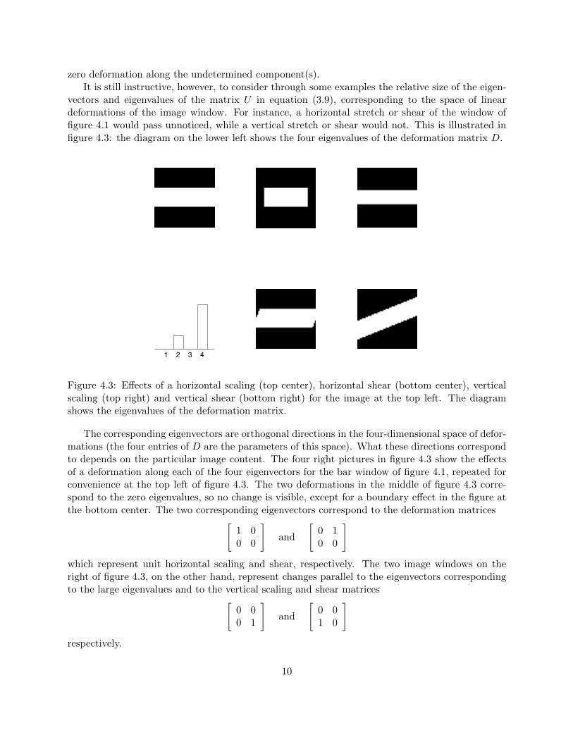
vectors and eigenvalues of the matrix U in equation (3.9), corresponding to the space of lineardeformations of the image window. For instance, a horizontal stretch or shear of the window offigure 4.1 would pass unnoticed, while a vertical stretch or shear would not. This is illustrated infigure 4.3: the diagram on the lower left shows the four eigenvalues of the deformation matrix D.

21 3 4

Figure 4.3: Effects of a horizontal scaling (top center), horizontal shear (bottom center), verticalscaling (top right) and vertical shear (bottom right) for the image at the top left. The diagramshows the eigenvalues of the deformation matrix.

The corresponding eigenvectors are orthogonal directions in the four-dimensional space of defor-mations (the four entries of D are the parameters of this space). What these directions correspondto depends on the particular image content. The four right pictures in figure 4.3 show the effectsof a deformation along each of the four eigenvectors for the bar window of figure 4.1, repeated forconvenience at the top left of figure 4.3. The two deformations in the middle of figure 4.3 corre-spond to the zero eigenvalues, so no change is visible, except for a boundary effect in the figure atthe bottom center. The two corresponding eigenvectors correspond to the deformation matrices[

1 00 0

]and

[0 10 0

]which represent unit horizontal scaling and shear, respectively. The two image windows on theright of figure 4.3, on the other hand, represent changes parallel to the eigenvectors correspondingto the large eigenvalues and to the vertical scaling and shear matrices[

0 00 1

]and

[0 01 0

]respectively.

10

4321

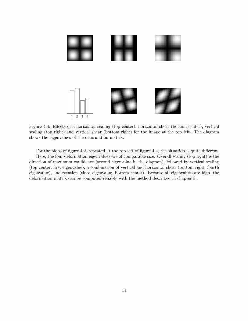
Figure 4.4: Effects of a horizontal scaling (top center), horizontal shear (bottom center), verticalscaling (top right) and vertical shear (bottom right) for the image at the top left. The diagramshows the eigenvalues of the deformation matrix.

For the blobs of figure 4.2, repeated at the top left of figure 4.4, the situation is quite different.Here, the four deformation eigenvalues are of comparable size. Overall scaling (top right) is the

direction of maximum confidence (second eigenvalue in the diagram), followed by vertical scaling(top center, first eigenvalue), a combination of vertical and horizontal shear (bottom right, fourtheigenvalue), and rotation (third eigenvalue, bottom center). Because all eigenvalues are high, thedeformation matrix can be computed reliably with the method described in chapter 3.

11

Chapter 5

Dissimilarity

A feature with a high measure of confidence, as defined in the previous chapter, can still be abad feature to track. For instance, in an image of a tree, a horizontal twig in the foreground canintersect a vertical twig in the background. This intersection, however, occurs only in the image,not in the world, since the two twigs are at different depths. Any selection criterion would pick theintersection as a good feature to track, and yet there is no real world feature there to speak of. Theproblem is that image feature and world feature do not necessarily coincide, and an image windowjust does not contain enough information to determine whether an image feature is also a featurein the world.

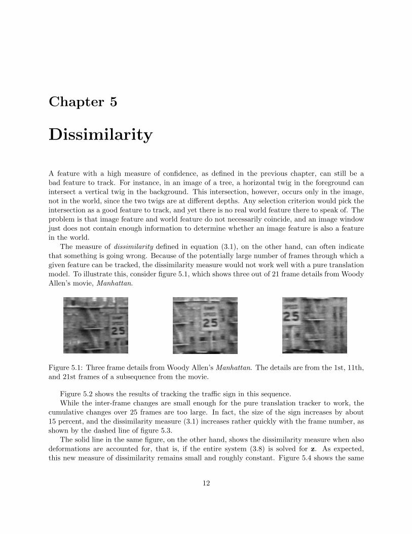
The measure of dissimilarity defined in equation (3.1), on the other hand, can often indicatethat something is going wrong. Because of the potentially large number of frames through which agiven feature can be tracked, the dissimilarity measure would not work well with a pure translationmodel. To illustrate this, consider figure 5.1, which shows three out of 21 frame details from WoodyAllen’s movie, Manhattan.

Figure 5.1: Three frame details from Woody Allen’s Manhattan. The details are from the 1st, 11th,and 21st frames of a subsequence from the movie.

Figure 5.2 shows the results of tracking the traffic sign in this sequence.While the inter-frame changes are small enough for the pure translation tracker to work, the

cumulative changes over 25 frames are too large. In fact, the size of the sign increases by about15 percent, and the dissimilarity measure (3.1) increases rather quickly with the frame number, asshown by the dashed line of figure 5.3.

The solid line in the same figure, on the other hand, shows the dissimilarity measure when alsodeformations are accounted for, that is, if the entire system (3.8) is solved for z. As expected,this new measure of dissimilarity remains small and roughly constant. Figure 5.4 shows the same

12

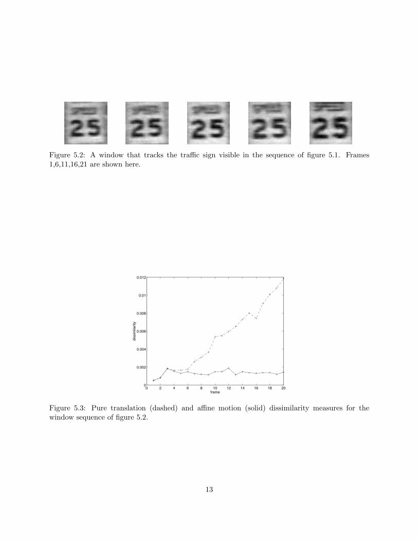
Figure 5.2: A window that tracks the traffic sign visible in the sequence of figure 5.1. Frames1,6,11,16,21 are shown here.

0 2 4 6 8 10 12 14 16 18 200

0.002

0.004

0.006

0.008

0.01

0.012

frame

dissimilarity

Figure 5.3: Pure translation (dashed) and affine motion (solid) dissimilarity measures for thewindow sequence of figure 5.2.

13

windows as in figure 5.2, but warped by the computed deformations. The deformations make thefive windows virtually equal to each other.

Figure 5.4: The same windows as in figure 5.2, warped by the computed deformation matrices.

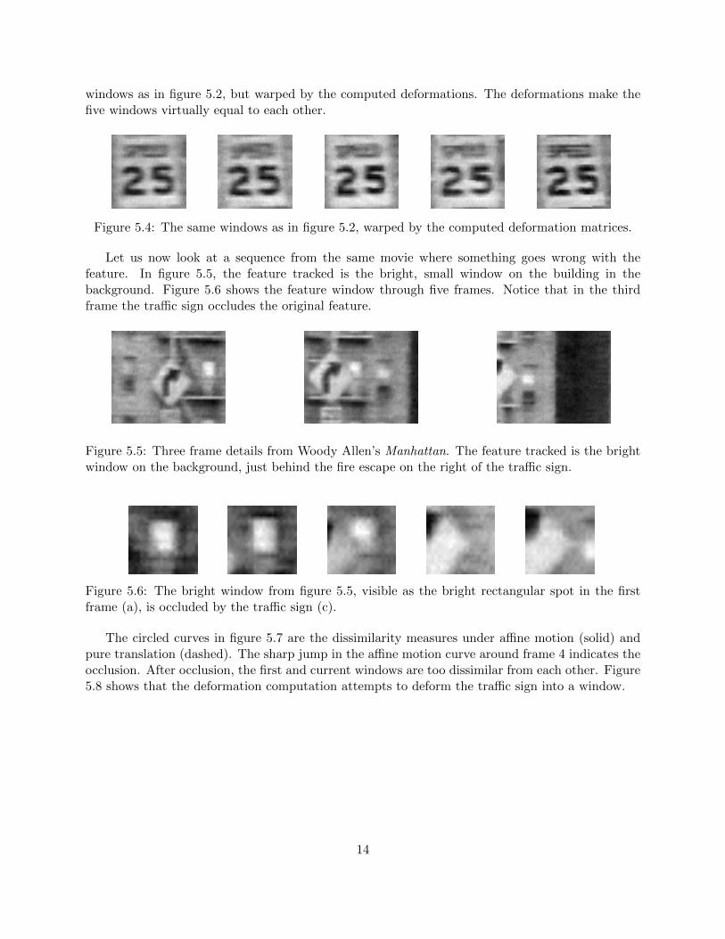
Let us now look at a sequence from the same movie where something goes wrong with thefeature. In figure 5.5, the feature tracked is the bright, small window on the building in thebackground. Figure 5.6 shows the feature window through five frames. Notice that in the thirdframe the traffic sign occludes the original feature.

Figure 5.5: Three frame details from Woody Allen’s Manhattan. The feature tracked is the brightwindow on the background, just behind the fire escape on the right of the traffic sign.

Figure 5.6: The bright window from figure 5.5, visible as the bright rectangular spot in the firstframe (a), is occluded by the traffic sign (c).

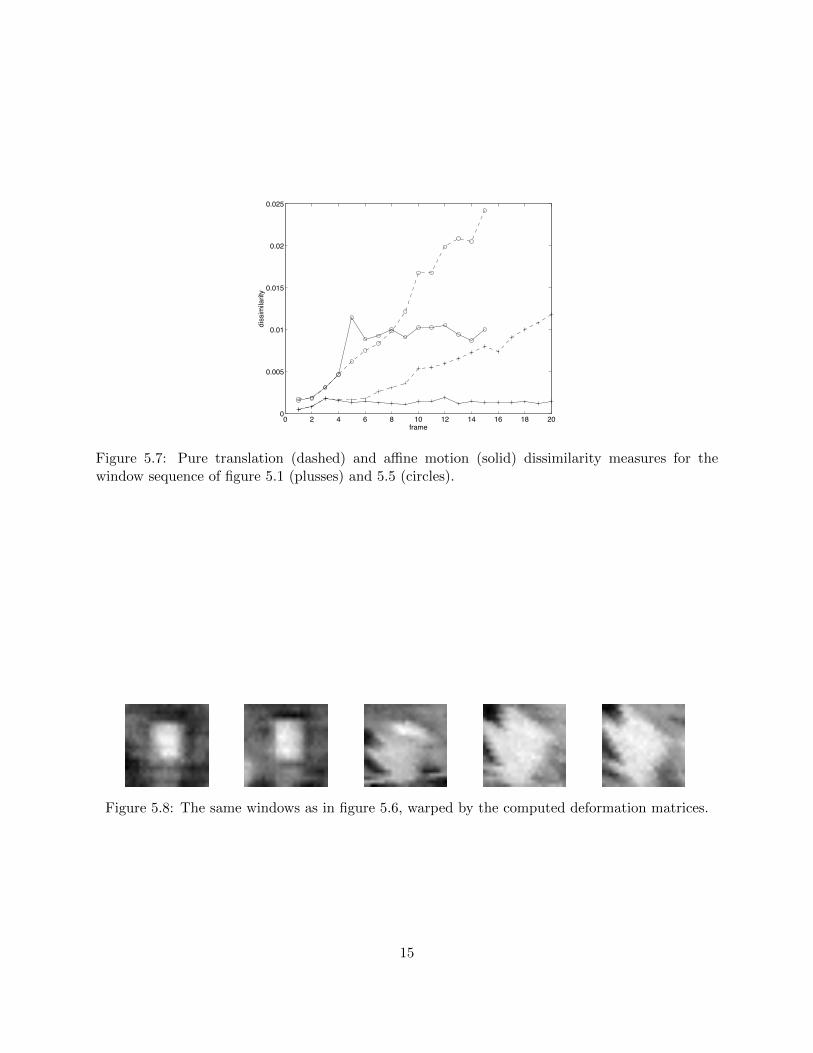
The circled curves in figure 5.7 are the dissimilarity measures under affine motion (solid) andpure translation (dashed). The sharp jump in the affine motion curve around frame 4 indicates theocclusion. After occlusion, the first and current windows are too dissimilar from each other. Figure5.8 shows that the deformation computation attempts to deform the traffic sign into a window.

14

0 2 4 6 8 10 12 14 16 18 200

0.005

0.01

0.015

0.02

0.025

frame

dissimilarity

Figure 5.7: Pure translation (dashed) and affine motion (solid) dissimilarity measures for thewindow sequence of figure 5.1 (plusses) and 5.5 (circles).

Figure 5.8: The same windows as in figure 5.6, warped by the computed deformation matrices.

15

Chapter 6

Simulations

In this chapter, we present simulation results to show that if the affine motion model is correctthen the tracking algorithm presented in chapter 3 converges even when the starting point is farremoved from the true solution.

The first series of simulations are run on the four circular blobs we considered in chapter 4(figure 4.2). The following three motions are considered:

D1 =

[1.4095 −0.34200.3420 0.5638

], d1 =

[30

]

D2 =

[0.6578 −0.34200.3420 0.6578

], d2 =

[20

]

D3 =

[0.8090 0.25340.3423 1.2320

], d3 =

[30

]

To see the effects of these motions, compare the first and last column of figure 6.1. The imagesin the first column are the feature windows in the first image (equal for all three simulations in thisseries), while the images in the last column are the images warped and translated by the motionsspecified above and corrupted with random Gaussian noise with a standard deviation equal to 16percent of the maximum image intensity. The images in the intermediate columns are the resultsof the deformations and translations to which the tracking algorithm subjects the images in theleftmost column after 4, 8, and 19 iterations, respectively. If the algorithm works correctly, theimages in the fourth column of figure 6.1 should be as similar as possible to those in the fifthcolumn, which is indeed the case.

A more quantitative idea of the convergence of the tracking algorithm is given by figure 6.2,which plots the dissimilarity measure, translation error, and deformation error as a function of theframe number (first three columns), as well as the intermediate displacements and deformations(last two columns). Deformations are represented in the fifth column of figure 6.2 by two vectorseach, corresponding to the two columns of the transformation matrix A = 1 + D. Displacementsand displacement errors are in pixels, while deformation errors are the Frobenius norms of thedifference between true and computed deformation matrices. Table 6.1 shows the numerical valuesof true and computed deformations and translations.

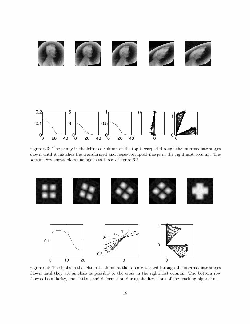
Figure 6.3 shows a similar experiment with a more complex image, the image of a penny(available in Matlab). Finally, figure 6.4 shows the result of attempting to match two completely

16

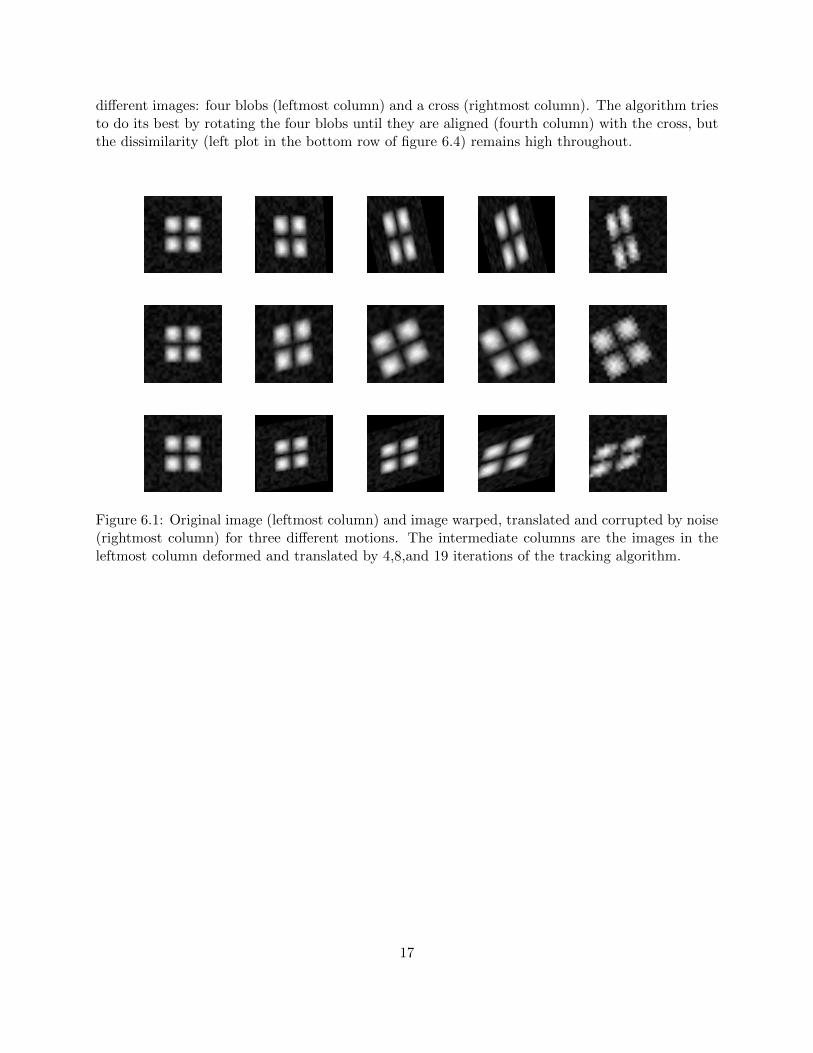
different images: four blobs (leftmost column) and a cross (rightmost column). The algorithm triesto do its best by rotating the four blobs until they are aligned (fourth column) with the cross, butthe dissimilarity (left plot in the bottom row of figure 6.4) remains high throughout.

Figure 6.1: Original image (leftmost column) and image warped, translated and corrupted by noise(rightmost column) for three different motions. The intermediate columns are the images in theleftmost column deformed and translated by 4,8,and 19 iterations of the tracking algorithm.

17

0 10 200

0.05

0.1

0 10 200

0.5

1

0 10 200

1.5

3

0

0

0 3

0

0 10 200

0.05

0.1

0 10 200

0.5

1

0 10 200

1.5

3

0 10

0 1.5

0

0 10 200

0.05

0.1

0 10 200

0.5

0 10 200

1.5

3

00

1

0 3

0

Figure 6.2: The first three columns show the dissimilarity, displacement error, and deformation erroras a function of the tracking algorithm’s iteration number. The last two columns are displacementsand deformations computed during tracking, starting from zero displacement and deformation.

Simulation True Computed True ComputedNumber Deformation Deformation Translation Translation

1

[1.4095 −0.34200.3420 0.5638

] [1.3930 −0.33430.3381 0.5691

] [30

] [3.0785−0.0007

]

2

[0.6578 −0.34200.3420 0.6578

] [0.6699 −0.34320.3187 0.6605

] [20

] [2.09200.0155

]

3

[0.8090 0.25340.3423 1.2320

] [0.8018 0.23500.3507 1.2274

] [30

] [3.05910.0342

]

Table 6.1: Comparison of true and computed deformations and displacements (in pixels) for thethree simulations illustrated in figures 6.1 and 6.2.

18

0 20 400

0.1

0.2

0 20 400

0.5

1

0 20 400

3

6

00

1

0

0

Figure 6.3: The penny in the leftmost column at the top is warped through the intermediate stagesshown until it matches the transformed and noise-corrupted image in the rightmost column. Thebottom row shows plots analogous to those of figure 6.2.

0 10 20

0.1

0

0

1

0-0.6

0

Figure 6.4: The blobs in the leftmost column at the top are warped through the intermediate stagesshown until they are as close as possible to the cross in the rightmost column. The bottom rowshows dissimilarity, translation, and deformation during the iterations of the tracking algorithm.

19

Chapter 7

More Experiments on Real Images

The experiments and simulations of the previous chapters illustrate specific points and issues con-cerning feature monitoring and tracking. Whether the feature selection and monitoring proposedin this report are useful, on the other hand, can only be established by more extensive experimentson more images and larger populations of features. The experiments in this chapter are a step inthat direction.

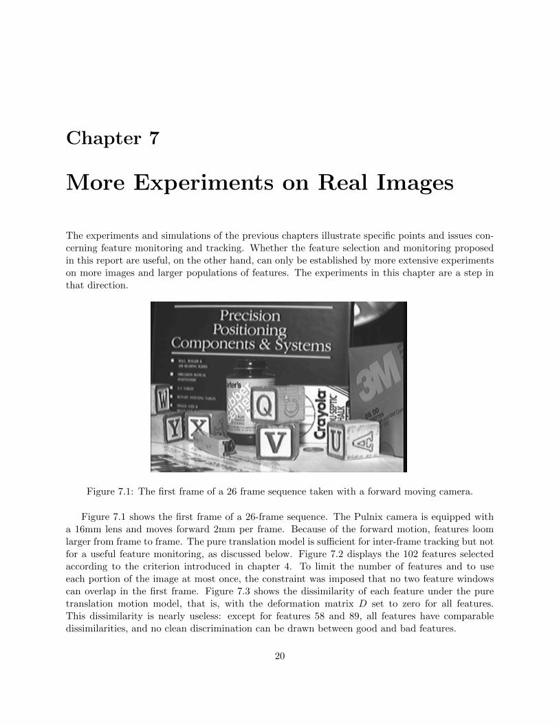
Figure 7.1: The first frame of a 26 frame sequence taken with a forward moving camera.

Figure 7.1 shows the first frame of a 26-frame sequence. The Pulnix camera is equipped witha 16mm lens and moves forward 2mm per frame. Because of the forward motion, features loomlarger from frame to frame. The pure translation model is sufficient for inter-frame tracking but notfor a useful feature monitoring, as discussed below. Figure 7.2 displays the 102 features selectedaccording to the criterion introduced in chapter 4. To limit the number of features and to useeach portion of the image at most once, the constraint was imposed that no two feature windowscan overlap in the first frame. Figure 7.3 shows the dissimilarity of each feature under the puretranslation motion model, that is, with the deformation matrix D set to zero for all features.This dissimilarity is nearly useless: except for features 58 and 89, all features have comparabledissimilarities, and no clean discrimination can be drawn between good and bad features.

20

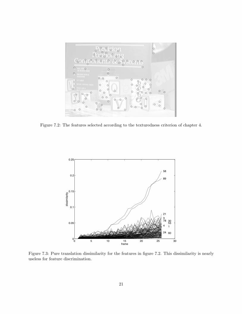
Figure 7.2: The features selected according to the texturedness criterion of chapter 4.

0 5 10 15 20 25 300

0.05

0.1

0.15

0.2

0.25

frame

dissimilarity

89

58

78

213

4

24

30

1

60

53

Figure 7.3: Pure translation dissimilarity for the features in figure 7.2. This dissimilarity is nearlyuseless for feature discrimination.

21

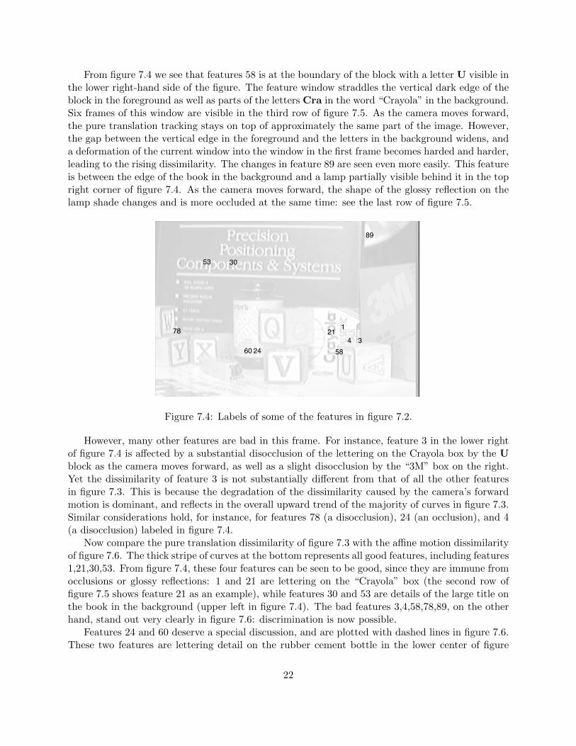
From figure 7.4 we see that features 58 is at the boundary of the block with a letter U visible inthe lower right-hand side of the figure. The feature window straddles the vertical dark edge of theblock in the foreground as well as parts of the letters Cra in the word “Crayola” in the background.Six frames of this window are visible in the third row of figure 7.5. As the camera moves forward,the pure translation tracking stays on top of approximately the same part of the image. However,the gap between the vertical edge in the foreground and the letters in the background widens, anda deformation of the current window into the window in the first frame becomes harded and harder,leading to the rising dissimilarity. The changes in feature 89 are seen even more easily. This featureis between the edge of the book in the background and a lamp partially visible behind it in the topright corner of figure 7.4. As the camera moves forward, the shape of the glossy reflection on thelamp shade changes and is more occluded at the same time: see the last row of figure 7.5.

89

58

78

60 2434

21

53 30

1

Figure 7.4: Labels of some of the features in figure 7.2.

However, many other features are bad in this frame. For instance, feature 3 in the lower rightof figure 7.4 is affected by a substantial disocclusion of the lettering on the Crayola box by the Ublock as the camera moves forward, as well as a slight disocclusion by the “3M” box on the right.Yet the dissimilarity of feature 3 is not substantially different from that of all the other featuresin figure 7.3. This is because the degradation of the dissimilarity caused by the camera’s forwardmotion is dominant, and reflects in the overall upward trend of the majority of curves in figure 7.3.Similar considerations hold, for instance, for features 78 (a disocclusion), 24 (an occlusion), and 4(a disocclusion) labeled in figure 7.4.

Now compare the pure translation dissimilarity of figure 7.3 with the affine motion dissimilarityof figure 7.6. The thick stripe of curves at the bottom represents all good features, including features1,21,30,53. From figure 7.4, these four features can be seen to be good, since they are immune fromocclusions or glossy reflections: 1 and 21 are lettering on the “Crayola” box (the second row offigure 7.5 shows feature 21 as an example), while features 30 and 53 are details of the large title onthe book in the background (upper left in figure 7.4). The bad features 3,4,58,78,89, on the otherhand, stand out very clearly in figure 7.6: discrimination is now possible.

Features 24 and 60 deserve a special discussion, and are plotted with dashed lines in figure 7.6.These two features are lettering detail on the rubber cement bottle in the lower center of figure

22

1

89

6 11 16 21 26

3

21

58

60

78

Figure 7.5: Six sample features through six sample frames.

0 5 10 15 20 25 300

0.005

0.01

0.015

0.02

0.025

0.03

0.035

0.04

0.045

0.05

frame

dissimilarity

8958

78

21

34

6024

53130

Figure 7.6: Affine motion dissimilarity for the features in figure 7.2. Notice the good discriminationbetween good and bad features. Dashed plots indicate aliasing (see text).

23

7.4. The fourth row of figure 7.5 shows feature 60 as an example. Although feature 24 has anadditional slight occlusion as the camera moves forward, these two features stand out from the verybeginning, that is, even for very low frame numbers in figure 7.6, and their dissimilarity curves arevery erratic throughout the sequence. This is because of aliasing: from the fourth row of figure 7.5,we see that feature 60 (and similarly feature 24) contains very small lettering, of size comparableto the image’s pixel size (the feature window is 25 × 25 pixels). The matching between one frameand the next is haphazard, because the characters in the lettering are badly aliased. This behavioris not a problem: erratic dissimilarities indicate trouble, and the corresponding features ought tobe abandoned.

24

Chapter 8

Conclusion

In this report, we have proposed both a method for feature selection and a technique for featuremonitoring during tracking. Selection specifically maximizes the quality of tracking, and is thereforeoptimal by construction, as opposed to more ad hoc measures of texturedness. Monitoring iscomputationally inexpensive and sound, and makes it possible to discriminate between good andbad features based on a measure of dissimilarity that uses affine motion as the underlying imagechange model.

Of course, monitoring feature dissimilarity does not solve all the problems of tracking. In somesituations, a bright spot on a glossy surface is a bad (that is, nonrigid) feature, but may changelittle over a long sequence: dissimilarity may not detect the problem. However, it must be realizedthat not everything can be decided locally. For the case in point, rigidity is not a local feature, soa local method cannot be expected to detect its violation. On the other hand, many problems canindeed be discovered locally and these are the target of the investigation in this report. The manyillustrative experiments and simulations, as well as the large experiment of chapter 7, show thatmonitoring is indeed effective in realistic circumstances. A good discrimination at the beginning ofthe processing chain can reduce the remaining bad features to a few outliers, rather than leavingthem an overwhelming majority. Outlier detection techniques at higher levels in the processingchain are then much more likely to succeed.

25

Bibliography

[Ana89] P. Anandan. A computational framework and an algorithm for the measurement of visualmotion. International Journal of Computer Vision, 2(3):283–310, January 1989.

[BYX82] P. J. Burt, C. Yen, and X. Xu. Local correlation measures for motion analysis: a com-parative study. In Proceedings of the IEEE Conference on Pattern Recognition and ImageProcessing, pages 269–274, 1982.

[CL74] D. J. Connor and J. O. Limb. Properties of frame-difference signals generated by movingimages. IEEE Transactions on Communications, COM-22(10):1564–1575, October 1974.

[CR76] C. Cafforio and F. Rocca. Methods for measuring small displacements in television images.IEEE Transactions on Information Theory, IT-22:573–579, 1976.

[DN81] L. Dreschler and H.-H. Nagel. Volumetric model and 3d trajectory of a moving car derivedfrom monocular tv frame sequences of a street scene. In Proceedings of the InternationalJoint Conference on Artificial Intelligence, pages 692–697, Vancouver, Canada, August1981.

[F8̈7] W. Foerstner. Reliability analysis of parameter estimation in linear models with applica-tions to mansuration problems in computer vision. Computer Vision, Graphics, and ImageProcessing, 40:273–310, 1987.

[FM91] C. S. Fuh and P. Maragos. Motion displacement estimation using and affine model formatching. Optical Engineering, 30(7):881–887, July 1991.

[FP86] W. Foerstner and A. Pertl. Photogrammetric Standard Methods and Digital Image Match-ing Techniques for High Precision Surface Measurements. Elsevier Science Publishers,1986.

[KR80] L. Kitchen and A. Rosenfeld. Gray-level corner detection. Computer Science Center 887,University of Maryland, College Park, April 1980.

[LK81] B. D. Lucas and T. Kanade. An iterative image registration technique with an applicationto stereo vision. In Proceedings of the 7th International Joint Conference on ArtificialIntelligence, 1981.

[MO93] R. Manmatha and John Oliensis. Extracting affine deformations from image patches - i:Finding scale and rotation. In Proceedings of the IEEE Conference on Computer Visionand Pattern Recognition, pages 754–755, 1993.

26

[Mor80] H. Moravec. Obstacle avoidance and navigation in the real world by a seeing robot rover.PhD thesis, Stanford University, September 1980.

[MPU79] D. Marr, T. Poggio, and S. Ullman. Bandpass channels, zero-crossings, and early visualinformation processing. Journal of the Optical Society of America, 69:914–916, 1979.

[OK92] M. Okutomi and T. Kanade. A locally adaptive window for signal matching. InternationalJournal of Computer Vision, 7(2):143–162, January 1992.

[RGH80] T. W. Ryan, R. T. Gray, and B. R. Hunt. Prediction of correlation errors in stereo-pairimages. Optical Engineering, 19(3):312–322, 1980.

[TH86] Q. Tian and M. N. Huhns. Algorithms for subpixel registration. Computer Vision, Graph-ics, and Image Processing, 35:220–233, 1986.

[Van92] C. Van Loan. Computational Frameworks for the Fast Fourier Transform. Frontiers inApplied Mathematics. SIAM, Philadelphia, PA, 1992.

[Woo83] G. A. Wood. Realities of automatic correlation problem. Photogrammetric Engineeringand Remote Sensing, 49:537–538, April 1983.

27

Appendix A

Derivation of the Tracking Equation

In this appendix, we derive the basic tracking equation (3.8) by rewriting equations (3.6) and (3.7)in a matrix form that clearly separates unknowns from known parameters. The necessary algebraicmanipulation can be done cleanly by using the Kronecker product defined as follows [Van92]. If Ais a p× q matrix and B is m× n, then the Kronecker product A⊗B is the p× q block matrix

A⊗B =

a11B · · · a1qB...

...ap1B · · · apqB

of size pm × qn. For any p × q matrix A, let now v(A) be a vector collecting the entries of A incolumn-major order:

v(A) =

a11a21...apq

so in particular for a vector or a scalar xwe have v(x) = x). Given three matrices A,X,B for whichthe product AXB is defined, the following two equalities are then easily verified:

AT ⊗BT = (A⊗B)T (A.1)

v(AXB) = (BT ⊗A)v(X) . (A.2)

The last equality allows us to “pull out” the unknowns D and d from equations (3.6) and (3.7).The scalar term gTu appears in both equations (3.6) and (3.7). By using the identities (A.1),

(A.2), and definition 3.4, we can write

gTu = gT (Dx + d)

= gTDx + gTd

= v(gTDx) + gTd

= (xT ⊗ gT )v(D) + gTd

= (x ⊗ g)T v(D) + gTd .

28

Similarly, the vectorized version of the 2 × 2 matrix gxT that appears in equation (3.6) is

v(gxT ) = v(g 1 xT )

= x ⊗ g .

We can now vectorize matrix equation (3.6) into the following vector equation:(∫ ∫WU(x)w dx

)v(D) +

(∫ ∫WV (x)w dx

)d =

∫ ∫W

b(x)w dx (A.3)

where the rank 1 matrices U and V and the vector b are defined as follows:

U(x) = (x ⊗ g)(x ⊗ g)T

V (x) = (x ⊗ g)gT

b(x) = [I(x) − J(x)] v(gxT ) .

Similarly, equation (3.7) can be written as(∫ ∫WV T (x)w dx

)v(D) +

(∫ ∫WZ(x)w dx

)d =

∫ ∫W

c(x)w dx (A.4)

where V has been defined above and the rank 1 matrix Z and the vector c are defined as follows:

Z(x) = ggT

c(x) = [I(x) − J(x)] g .

Equations (A.3) and (A.4) can be summarized by introducing the symmetric 6 × 6 matrix

T =

∫ ∫W

[U VV T Z

]w dx

=

∫ ∫W

x2g2x x2gxgy xyg2x xygxgy xg2x xgxgyx2gxgy x2g2y xygxgy xyg2y xgxgy xg2yxyg2x xygxgy y2g2x y2gxgy yg2x ygxgyxygxgy xyg2y y2gxgy y2g2y ygxgy yg2yxg2x xgxgy yg2x ygxgy g2x gxgyxgxgy xg2y ygxgy yg2y gxgy g2y

w dx ,

the 6 × 1 vector of unknowns

z =

[v(D)

d

],

and the 6 × 1 vector

a =

∫ ∫W

[bc

]w dx

=

∫ ∫W

[I(x) − J(x)]

xgxxgyygxygygxgy

w dx .

29

With this notation, the basic step of the iterative procedure for the computation of affinedeformation D and translation d is the solution of the following linear 6 × 6 system:

Tz = a .

30