gonzalo garc a-donato - vabarvabar.es/assets/scova16/garciadonato-talk.pdf · bayesian methods for...

Bayesian methods for Model Selection and related problems

Gonzalo Garcıa-Donato

Universidad de Castilla-La Mancha (Spain) and VaBar

ScoVa16-Valencia

google: garcia-donato ScoVa16-Valencia 1 / 28

VaBar and model selection

Model Selection, MS, has been a main line of research of our group during the last15 years.

Our work is greatly influenced by two prominent Bayesians: Susie Bayarri and JimBerger.

Our paradigm is objective Bayesian.

Regarding the relation MS-VaBar, this talk presents the problem, reviews what wehave done (past), briefly introduce current lines of research (present).

The objective is call your attention to this fascinating problem and, why not,capturing your interest to collaborate in the next years.... simBIOSSis and let uswrite the future!


1 Introducing the problem

2 Our view and what we have done

3 What we are doing now


Introducing the problem






Model selection

• Model Selection (or model choice), a definition: statistical problem where severalstatistical models

M1(y | θ1), M2(y | θ2), . . . ,Mk(y | θk),

are considered as plausible explanations for an experiment with output y .

Keyword is model uncertainty

since it is unknown which is the true model and that uncertainty is explicitly considered.

• The set of competing models is called the model space and usually is denoted as M.• Possible specific MS goals:

To choose a single model (which is the true model?),

To explicitly incorporate model uncertainty to provide more realisticinferences/predictions (this is called Model Averaging), a problem sometimespresented as mixture modeling.

• Two particular (and very popular) MS problems

• Hypothesis testing, and • Variable selection



Hypothesis testing

• In testing, the competing models have a common statistical form, say M(y | θ), butdiffer on where θ is located

Mi (y | θi ) = {M(y | θ = θi ), θi ∈ Θi}, i = 1, . . . , k,

normally denoted asHi : θ ∈ Θi , i = 1, . . . , k.

• Particularly popular/important/difficult is the testing problem with some of Θi

consisting on a single point in the corresponding Euclidean space (e.g. θ = 0). Thistesting problem is normally called point or precise.



Variable selection

Variable selection

• Model selection problems where the different models, Mi differ about which variables ofa given set x1, x2, . . . , xp explains a response variable y .

Variable selection is a multiple testing problem with 2p (precise) hypotheses of the type

Hi : βj1 = · · · = βjk = 0.


Our view and what we have done


2 Our view and what we have doneThe Bayesian answer :) and related aspects :(Our contributions to the MS problem: the present



Our view and what we have done The Bayesian answer :) and related aspects :(






Posterior model probabilities

• The formal Bayesian answer to the MS problem is based on the posterior probabilitiesof the competing models:

Pr(Mj | y)

• Such (discrete) posterior distribution encapsulates the responses to every question inModel Selection. Two examples:

If you want to select a single model use the most probable a posteriori and report itsposterior probability as a measure of uncertainty.

Model averaging? Use Pr(Mj | y) as weights.



Posterior model probabilities and Bayes factors

Assuming one of the models in M is the true model

Pr(Mj | y) =mj(y)Pr(Mj)∑i mi (y)Pr(Mi )

=Bj0Pr(Mj)∑i Bi0Pr(Mi )

,

where

Ingredient Name Type of problemmi (y) =

∫Mi (y | θi )πi (θi ) dθi prior marginal Computational

Bi0 Bayes factor of Mi to M0 NonePr(Mi ) prior prob. of Mi MultiplicityC Normalizing constant Computationalπi (θi ) prior for Mi All sort of problems



πi (θi ): the main conceptual challenge

MS prior distributions are, perhaps, the most problematic aspect of any Bayesianapproach. In MS the difficulties grow:

Results are very sensitive to the prior distribution (changing the prior you canessentially obtain whatever you want).

Such sensitiveness does not disappear asymptotically with n.

Neither improper nor vague priors can be used.

Frequentist properties are not very useful to differentiate among priors (and arepotentially misleading)


Our view and what we have done Our contributions to the MS problem: the present






Contributions (I): About πi (θi )

Our contributions about πi have roots on Jeffreys who first proposed using proper priorscentered at the ‘null’ and with flat tails (Cauchy). Zellner and Siow (1980) extended thisidea to regression problems.

Bayarri and Garcia-Donato (2007), used such priors to test general hypotheses inlinear models (regression or ANOVA).

Bayarri and Garcia-Donato (2008), propose a general mathematical rule that extendJeffreys’ priors to any other testing problem. These are named as Divergence Basedpriors.

Bayarri, Berger, Forte and Garcia-Donato (2012), introduce a deep methodologicalchange. They propose and formalize the idea of specifying (and characterizing)priors based on sensible criteria like invariance, predictive matching and consistency.

The method is illustrated proposing a new prior for variable selection in linearmodels with optimal properties that they call Robust prior.



Contributions (II): Computational aspects

The number of competing models in variable selection, 2p, becomes easily very, very large.Posterior probabilities cannot be exactly computed and heuristic methods are called for.

Garcia-Donato and Martinez-Beneito (2013), show that very simple Gibbs algorithmsplus frequency of visits to estimate probabilities, largely outperforms modernsearching methods with estimations based on re-normalization.

1 2 3 4 5

0.00.2

0.40.6

0.81.0

Ozone35

Run

Prob(X

tXh|y)

Gibbs+EmpiricalBAS+RenormalizedSSBM+Renormalized



Contributions (III): Software

The high specificity of the MS problem jointly with the particularities of its priors makesalmost useless standard Bayesian software (of the type WinBUGS, etc)

• Forte and Garcia-Donato (2012) have developed BayesVarSel, an R-package thatsolves testing and variable selection problems in linear models.Main characteristics:

Priors: ”Robust”, ”g-Zellner”, ”Zellner-Siow”, ”Liang”.

Priors for Mi : ”Constant”, ”ScottBerger”.

Methods: exact (sequential or parallel) and the empirical Gibbs here cited.

Results: HPM, inclusion probabilities (univariate, joint, conditionals), image plots,etc.

And with a simple and familiar (lm-type) interface:>Bvs(formula="IMC~ .", data=obesity, n.keep=1000)



Contributions (IV): Applications

Does it have real applications?

Determining the number of jointpoints in epidemiological temporal series(Martinez-Beneito and others in 2012).

Studying which factors explain the Gross Domestic Product in the US (Forte andothers in 2015).


What we are doing now



3 What we are doing nowLarge p small n problemOther projects in progress


What we are doing now Large p small n problem






High dimensional setting

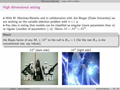
• With M. Martinez-Beneito and in collaboration with Jim Berger (Duke University) weare working on the variable selection problem with n << p.• Key idea is noting that models can be classified as singular (more parameters than n)or regular (number of parameters ≤ n). Hence M =MS ∪MR.

Result

the Bayes factor of any Mγ ∈MS to the null is Bγ0 = 1 (for the rest Bγ0 is theconventional one, say robust).

MS (dark side) MR (light side)



Who wins?

The scene now is that the dark side, MS , is a vast deserted (only ones) region while thelight side, MR , is a minuscule region lighted by the data.• eg. if p = 8408 and n = 41, the proportion of regular models over the total number ofmodels is of the order 10−2000.

The relevance a posteriori of singular models is

PS = Pr(MT ∈MS | y) =p − n + 1

p − n + 1 + n CR ,

where CR is the normalizing constant conditionally on MR .



The methodology in practice

No need to ‘explore’ the whole model space, it suffices with

exploring MR (still moderate to large: MCMC in Garcia-Donato andMartinez-Beneito, 2013),

estimating CR (George and McCulloch, 1997) and hence PS ,

any relevant feature of the posterior distribution can be easily computed.



An illustrative example

Simulated experiment in Hans et al (2007), with n = 41 patients and p = 8408 genesfrom a tumor specimen. The ‘true’ data generating model is

yi = 1.3xi1 + .3xi2 − 1.2xi3 − .5xi4 + N(0, 0.5).

We obtain:

n PS q1 q2 q3 q4 q−T qU−T HPM

41 0.004 0.843 0.154 0.766 0.002 0.002 0.038 {x1, x3}

30 0.320 0.300 0.171 0.173 0.160 0.159 0.251 {x1, x3}20 0.830 0.417 0.416 0.415 0.415 0.414 0.419 {x4026, x7748}10 0.995 0.497 0.497 0.497 0.497 0.497 0.497 {Null,Full}

Keys: qi is the inclusion probability for xi (i = 1, 2, 3, 4) and q−T , qU−T are respectively the mean

and maximum of the inclusion probabilities for the spurious variables. HPM is the estimated

most probable a posteriori model.


What we are doing now Other projects in progress






BayesVarSel vs. others

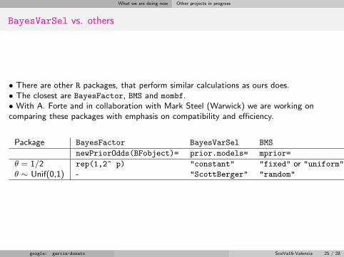
• There are other R packages, that perform similar calculations as ours does.• The closest are BayesFactor, BMS and mombf.• With A. Forte and in collaboration with Mark Steel (Warwick) we are working oncomparing these packages with emphasis on compatibility and efficiency.

Package BayesFactor BayesVarSel BMS mombf

newPriorOdds(BFobject)= prior.models= mprior= priorDelta=

θ = 1/2 rep(1,2^ p) "constant" "fixed" or "uniform" modelunifprior()

θ ∼ Unif(0,1) - "ScottBerger" "random" modelbbprior(1,1)



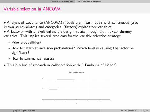
Variable selection in ANCOVA

• Analysis of Covariance (ANCOVA) models are linear models with continuous (alsoknown as covariates) and categorical (factors) explanatory variables.• A factor F with J levels enters the design matrix through x1, . . . , xJ−1 dummyvariables. This implies several problems for the variable selection strategy.

Prior probabilities?

How to interpret inclusion probabilities? Which level is causing the factor besignificant?

How to summarize results?

• This is a line of research in collaboration with R Paulo (U of Lisbon)

-2.0 -1.5 -1.0 -0.5 0.0 0.5 1.0

80% Credible regions

δ

δ2

δ3



Students

With A Forte and A Moro (master thesis work): The theory of the criteria paper,(Bayarri et al, 2012), although presented generically, was illustrated in normal Linearmodels. How does it apply in GLM’s?

With A Forte and E Moreno (thesis in progress): the problem with missing data invariable selection and summarizing the posterior distribution.

With A Forte and R Gavidia (thesis in progress): Variable selection in genomics.



VaBar and model selection

Thanks!


gonzalo garc a-donato - vabarvabar.es/assets/scova16/garciadonato-talk.pdf · bayesian methods for...

Documents