Has China Run out of Surplus Labour? 

Jane Golley1 and Xin Meng2

2011

Abstract:

Many recent studies claim that China has reached a Lewisian ‘turning point’ in economic development, signalled by rising wages in urban areas and the exhaustion of rural surplus labour. In this paper we show that despite some evidence of rising nominal urban unskilled wages between 2000 and 2009 there is little to suggest that this has been caused by unskilled labour supply shortage. China still has abundant workers who are under-employed with very low income in the rural sector. We argue that China’s unique institutional and policy-induced barriers to migration have prevented many rural workers from migrating to cities. Projections of the reduction in institutional barriers on supply of rural migrant workers through to 2020 demonstrate how much larger the migrant stock could be under alternative institutional settings.

1 Australian Centre on China in the World, CAP, Australian National University, Canberra, ACT 0200, Australia; email: jane.golley@anu.edu.au. 2 Corresponding author: Research School of Economics, CBE, Australian National University, Canberra, ACT 0200, Australia; email: xin.meng@anu.edu.au.

2

1. Introduction China has had three decades of unprecedented economic growth, which, to a significant extent, has been related to the large-scale movement of surplus labour from the low productivity rural sector to the high productivity urban sector. This migration has provided Chinese industries with cheap labour and facilitated the rapid growth of labour-intensive manufacturing exports concentrated along China’s south-eastern coastline, and in Guangdong in particular. Since 2004, news of labour shortages in Guangdong began to appear on the internet and in newspapers. Shortly after that, a number of academic studies emerged, claiming that China is either close to, or has already reached, a turning point in economic development in which rural surplus labour has been exhausted, resulting in labour shortages and rising wages in the urban sector (Garnaut and Huang, 2006; Cai and Wang, 2007a, and 2007b; Du and Wang, 2010).

This paper provides a range of empirical evidence to show that, despite some evidence of rising nominal wages in urban areas, there is little to suggest that this has been caused by a labour supply shortage. Instead, we show that China still has abundant workers who are under-employed with very low income in the rural sector, and we argue that it is China’s unique institutional and policy-induced barriers to migration that has prevented many of these workers from migrating to cities.

Whether China has run out of surplus labour has significant implications for China’s future pattern of economic growth and development. Critically, the appropriate policy responses to the end of China’s labour surplus are fundamentally different from those to address barriers to employment in the modern sectors of the economy. One such barrier stems from the fact that China’s rural migrants still operate under a guest worker system whereby migrants have limited or no access to the social welfare provisions available to the urban residents. This impacts negatively on rural residents’ migration decisions and therefore reduces rural workers’ willingness to migrate to urban areas. Thus potentially hundreds of millions of workers who are in fact surplus to requirements in the rural sector choose to stay there anyway, indicating not an ‘end of surplus labour’, but a discriminatory and segmented labour market instead. While others (such as Garnaut, 2010) have acknowledged this point, they have not conducted the empirical work to verify just how important it might be.

Much of the empirical work below draws on the survey conducted under the Rural-Urban Migration in China and Indonesia (RUMiCI) project, which commenced in 2008 and will run through to 2011. The survey covers three groups of Chinese households: 5000 urban migrant households who worked in 15 designated cities (migrant survey); 5000 urban local incumbent households in the same cities (urban household survey), and 8000 rural households with and without migrant members from the nine provinces where the 15 cities are located (rural household survey). The nine provinces or metropolitan areas are Shanghai, Guangdong, Jiangsu, Zhejiang, Anhui, Hubei, Sichuan, Chongqing and Henan. The first four of these are the largest migrant destinations, the remaining five are the largest migration sending areas. The RUMiCI survey of migrant workers in urban cities, to the best of our knowledge, is the only random sample of

3

migrant workers for China so far.3 The representative of the sample and the comprehensive nature of the data allow us to investigate our hypothesis from a range of different angles in a relatively consistent way.

The paper is structured as follows. The next sections summarises the theory of the turning point and the current debate as it applies to China. Section 3 focuses on the wage growth of Chinese urban unskilled workers between 2000 and 2009 to demonstrate that there is nothing about this growth that convincingly implies the exhaustion of migrant labour supply. Section 4 examines rural survey data to reveal low migration rates, substantial earnings differentials between rural migrants and both agricultural and non-agricultural rural workers, and an abundance of rural workers who are under-employed with extremely low earnings. In section 5 we conduct projections of the rural migrant workforce through to 2020 to demonstrate just how much larger the migrant stock could be under alternative hypothetical but plausible assumptions about future patterns of migration. Section 6 concludes the paper.

2. The current debate The theoretical starting point for this inquiry is the theory of the ‘turning point’, which was first developed by Arthur Lewis (1954), later refined by Ranis and Fei (1961) and Fei and Ranis (1964), and subsequently became one of the cornerstones of development economics. According to Lewis, in the early phase of economic development, an unlimited supply of unskilled rural labour from the ‘subsistence’, ‘traditional’ or agriculture sector is available for employment in the expanding ‘capitalist’, ‘modern’ or industrial sector. A significant proportion of this unskilled labour is ‘surplus’ in the sense that its marginal productivity is assumed to be below the subsistence wage, which in turn sets a wage floor in the capitalist sector. Thus drawing workers away from the subsistence sector has a negligible impact on output in that sector while enabling the expansion of the capitalist sector without any impact on wages, for as long as the surplus labour exists. Once the labour surplus runs out, however, wages begin to rise in both sectors, and inequalities between the two sectors begin to fall. This Lewisian turning point – or more accurately a turning period – necessitates structural change towards a more capital- and technology-intensive growth pattern, as evidenced by the growth experiences of most advanced economies.

Claims that China is either close to, or has already reached, this turning point in economic development are based on a number of inter-related points. First, some coastal urban areas have recorded double-digit wage growth in recent years, which has been coupled with anecdotal evidence of labour shortages in those areas. Even the wages of unskilled migrant workers rose strongly in the first decade of this century, according to Zhao and Wu (2007) and Du and Wang (2010). Second, as China’s population has entered a period of rapid aging, its ‘demographic dividend’ is coming to an end, implying a tightening of labour supply in the near future. Third, improvements in rural education

3 The detailed sampling procedure can be found in Meng and Manning (with Li and Tadjuddin) (2010) or at http://rumici.anu.edu.au.

 

4

have reduced the supply of unskilled workers (Cai, 2010, Du and Wang, 2010). Fourth, based on certain assumptions about the labour productivity and re-employability of rural workers, only 40 million people in the agriculture sector can actually be considered surplus labour (Cai, 2007b). Much of this work was recently published in a special issue of the China Economic Journal, published by the China Center for Economic Research at Peking University. According to Garnaut (2010a: 31), “data and analysis presented in [this special issue] suggest that the Chinese economy has now moved more decisively and deeply into the turning period”.

While some of these points are valid in their own right, whether or not they actually reveal that China has reached the turning point remains highly contentious, from a variety of different angles. In a ‘normal’ market economy (i.e., of the type Lewis was describing), the turning point may be identified by a sharp increase in wages in both the rural agricultural and urban industrial sectors, while there is also predicted to be a narrowing of the gap between the two. The wage increase should be most notable for unskilled workers in the urban sector, rather than for skilled workers who are not in direct competition with the largely unskilled pool of rural migrants. A key assumption is that labour markets are perfectly competitive, so that all workers are paid the value of their marginal product and that unskilled workers will be paid the same amount wherever they are employed. However, there are numerous reasons why the Chinese economy cannot yet be characterised in this sense as normal and why, therefore, rising wages in either sector may not indicate the arrival at the turning point but something else altogether.

As noted by World Bank (2007), the concentration of labour shortages in certain areas, and also in specific industries and companies, does not necessarily imply labour shortages more generally. Evidence of rapid wage growth based on aggregate wage statistics give an incomplete and biased picture, reflecting only official employment in state-owned enterprises and large private enterprises, while ignoring significant parts of the urban economy in which many low-skilled workers and migrants are employed. Even where the data is specifically for unskilled migrant workers (as in Du and Wang, 2010), failing to control for all the demand- and supply-side factors that may have contributed to rising wages risks attributing wage increases to labour shortages when they may in fact be due to, for example, higher productivity associated with an increasingly skilled workforce. Controlling for these other factors and using detailed factory-level data for the period 2000-2004, Meng and Bai (2007) show that average annual wage growth for unskilled migrant labour was, contrary to the findings of Du and Wang (2010), almost negligible. Evidence of urban labour market segmentation4 – with wage differentials existing across ownership, sectors, gender and between urban residents and rural migrants – further indicates that relying on aggregate official wage data may be misleading.

Meanwhile Cai’s (2007b) surplus of 40 million agriculture workers compares with more traditional estimates of 150-200 million (Brooks and Tao, 2003). His calculation assumes that over-40 year old rural workers lack the capacity to be re-employed in urban areas, which significantly reduces the rural migrant workforce in a 4 See Meng and Zhang, 2001, Démurger et al. 2007, 2009, Chen et al. 2007, Appleton et al., 2004 and Knight et al., 2001.

5

static sense. Even in this static sense, there is the potential to increase the capacity for re-employment in urban areas with policy efforts to re-train them (World Bank, 2007). In a dynamic sense, imagine a rural worker moving to a city in her early twenties, and rather than moving back home in her late twenties (as we show is a common trend below), she stays employed in the city through her forties, presumably reaching a productivity peak by then due to accumulated job experience. In this situation, she would certainly not lack the capacity to be employed in the city. In combination with potential increases in agriculture productivity, later retirement and increased labour force participation rates among older workers (which are currently very low), the amount of unskilled labour supply could be substantially higher than Cai suggests.5

Where Cai and Wang (2010) pinpoint 2004 as the commencement year for China’s turning point, Minami and Ma (2010) claim there is no evidence of a labour shortage in China and that the turning point has certainly not arrived there yet. They base this finding on estimates of agricultural production functions which they use to calculate the marginal productivity labour (MPL) in Chinese agriculture over the period 1990 to 2005, and also on the unemployment rate, which they claim to be “the most appropriate index to express the balance of labour demand and labour supply” (p. 164). Noting that beyond the turning point, an increasing MPL should lead to an acceleration of agricultural wage growth and a narrowing gap between rural and urban incomes and between unskilled and skilled wages, they go on to show that there was very little sign of any of these things happening up to 2007.

Minami and Ma (2010) are not the only ones on the ‘not yet’ side of the debate. Islam and Yokota (2008) use similar techniques to conclude that the turning point is approaching but has not arrived yet. Inagaki (2006), in his detailed examination of the extent of the labour shortage problem in coastal China, argues that the labour shortage is mainly concentrated on young female workers and in industries which employ young female workers. He concludes that improved labour conditions and the hiring of older female workers could prevent labour shortages, even in the longer run. Yao and Zhang (2010) estimate the supply and demand of migrant workers in each province during the period 1998-2007, and use these estimates in an endogenous switching model to estimate whether the national industrial wage lies on the upward-sloping or flat part of the industrial labour supply function. Finding that it is still on the latter (i.e., such that an increase in labour demand does not cause an increase in the wage rate), they conclude that the turning point has not yet been reached. Knight et al. (2010) use migrant household survey data for 2002 and 2007 to demonstrate that reports of migrant labour shortages and rising migrant wages can co-exist with a considerable pool of unskilled labour in the rural sector (some 80 million people in 2007). The two key reasons for this are the continuation of segmented labour markets and constraints to rural-urban migration.

In sum, a range of methods and data have been used to claim that China has already reached the turning point in economic development, yet a range of methods and data have also been used to claim that it has not. In what follows, we provide a critique of 5 See Golley and Tyers (2010) for evidence of the impact of higher labour force participation rates on China’s labour supply growth through to 2030.

6

some of the key findings in the former camp in combination with a range of evidence to support the latter.

3. Wage Growth of Urban Unskilled Workers

While the exhaustion of surplus labour is normally identified by a significant rise in wages of unskilled labour in the urban sector, in China the issue is more complicated. Due to segmentation in urban labour markets, urban workers are paid a premium for their urban residential status while migrant workers are often only allowed to access low-skilled jobs that are paid a lower market rate (Meng and Zheng, 2001). Thus it is important to examine trends in the wages of migrant workers, rather than urban workers, when investigating the turning point issue.

It is unfortunate that Chinese official statistics do not provide data on the wages of migrant workers. Some of the early advocates for the argument that China has reached the turning point rely on the wage data of urban residents (e.g., Garnaut and Huang, 2006 and Cai and Wang, 2007a), which basically misses the point. To overcome the problem that wages of urban residents do not reflect the labour supply situation of unskilled migrant workers, Cai and Wang (2007a) draw on data from the China Urban Labor Survey (CULS) for migrant and urban wage changes in five cities between 2001 and 2005 using two cross-sectional data sets with less than 1500 migrant workers and 3400 urban workers. They show that over this four-year period, the average nominal hourly earnings for migrants increased from 3.5 yuan/hour to 4.6 yuan/hour, while urban workers’ hourly wage increased from 5.7 to 6.8 yuan/hour. Based on these data they conclude that there is a serious shortage of unskilled labour because migrant wages increased more than urban resident wages.6

There are two major problems with the claims made by Cai and Wang (2007a). The first is that the CULS migrant survey suffers from sampling bias. Due to the fact that many migrant workers in China do not live in residential places, but in factory dormitories, construction sites or other workplaces, the residential-based CULS survey over samples self-employed migrant workers by a large margin. According to the 2005 one per cent population survey data, around 20 per cent of migrant workers are self-employed. The CULS 2001 survey, however, records that 54 per cent of workers are self-employed. It is therefore unclear whether the observed differential in earnings growth between migrants and urban residents is driven by the change in earnings of self-employed migrant workers, who tend to have relatively high ‘wages’ compared with other migrants as self-employed report their ‘net revenue’ rather than wages.

Second, the data used in Cai and Wang (2007a) are not from panel surveys, rather they are from two cross-sectional data sets. The change in average earnings calculated using these data may include changes in the composition of workers between the two data sets. For example, it is possible that the education level of workers in the 2001 sample is lower than that in the 2005 sample. If this is the case, the observed raw average wage increases cannot be attributed purely to labour supply shortages without controlling for 6 Zhao and Wu (2007) also provide average wage changes for migrant workers from records of their family members’ understanding for the years 2003 to 2006, indicating an annual increase in nominal monthly earnings between 4 and 8 per cent.

7

potential changes in the quality of labour input.

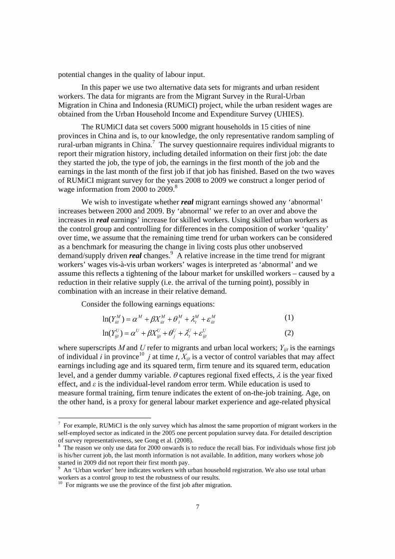
In this paper we use two alternative data sets for migrants and urban resident workers. The data for migrants are from the Migrant Survey in the Rural-Urban Migration in China and Indonesia (RUMiCI) project, while the urban resident wages are obtained from the Urban Household Income and Expenditure Survey (UHIES).

The RUMiCI data set covers 5000 migrant households in 15 cities of nine provinces in China and is, to our knowledge, the only representative random sampling of rural-urban migrants in China.7 The survey questionnaire requires individual migrants to report their migration history, including detailed information on their first job: the date they started the job, the type of job, the earnings in the first month of the job and the earnings in the last month of the first job if that job has finished. Based on the two waves of RUMiCI migrant survey for the years 2008 to 2009 we construct a longer period of wage information from 2000 to 2009.8

We wish to investigate whether real migrant earnings showed any ‘abnormal’ increases between 2000 and 2009. By ‘abnormal’ we refer to an over and above the increases in real earnings’ increase for skilled workers. Using skilled urban workers as the control group and controlling for differences in the composition of worker ‘quality’ over time, we assume that the remaining time trend for urban workers can be considered as a benchmark for measuring the change in living costs plus other unobserved demand/supply driven real changes.9 A relative increase in the time trend for migrant workers’ wages vis-à-vis urban workers’ wages is interpreted as ‘abnormal’ and we assume this reflects a tightening of the labour market for unskilled workers – caused by a reduction in their relative supply (i.e. the arrival of the turning point), possibly in combination with an increase in their relative demand.

Consider the following earnings equations:

ln(YijtM ) = α M + βXijt

M +θ jM + λt

M +ε ijtM (1)

ln(YijtU ) = αU + βXijt

U +θ jU + λt

U +ε ijtU (2)

where superscripts M and U refer to migrants and urban local workers; Yijt is the earnings of individual i in province10 j at time t, Xijt is a vector of control variables that may affect earnings including age and its squared term, firm tenure and its squared term, education level, and a gender dummy variable. θ captures regional fixed effects, λ is the year fixed effect, and ε is the individual-level random error term. While education is used to measure formal training, firm tenure indicates the extent of on-the-job training. Age, on the other hand, is a proxy for general labour market experience and age-related physical

7 For example, RUMiCI is the only survey which has almost the same proportion of migrant workers in the self-employed sector as indicated in the 2005 one percent population survey data. For detailed description of survey representativeness, see Gong et al. (2008). 8 The reason we only use data for 2000 onwards is to reduce the recall bias. For individuals whose first job is his/her current job, the last month information is not available. In addition, many workers whose job started in 2009 did not report their first month pay. 9 An ‘Urban worker’ here indicates workers with urban household registration. We also use total urban workers as a control group to test the robustness of our results. 10 For migrants we use the province of the first job after migration.

8

conditions such as eyesight and physical strength, which may affect labour productivity. Gender may to some extent capture labour market discrimination.

To investigate wage changes over time, the most important coefficients are the year fixed effects, λM and λU. In general λ captures changes in the cost of living over time, as well as any earnings’ increases driven by demand or supply changes that are not captured by the other observable factors. If over the period studied there is a significant tightening of unskilled migrant labour supply, we expect to observe an increase in λM /λU over time.

Before presenting the regression results, Figure 1 shows the log monthly earnings over the period 2000 to 2009 for urban skilled and migrant workers and the ratio of log monthly earnings for migrants to that for urban skilled workers (ln(YM)-ln(YU)). We use the average of first month and last month pay for each migrant’s first job, and use an occupation-based definition to classify skilled urban workers. The figure shows that migrant monthly earnings increased by less than 5 percent per annum (from log 6.45 to 6.92 in ten years), while for skilled urban workers the increase was over 10 percent per annum (from log 6.64 to 7.67). Over the ten-year period, therefore, we observe a significant rise in the earnings gap between the two groups, with migrant workers earning around 20 per cent less than skilled urban workers at the beginning of the period, and 75 per cent less at the end of the period. This certainly does not indicate a relative shortage of unskilled migrant workers, but would rather suggest a relative shortage of skilled urban workers – if we assume that changes in living costs for both groups were the same.

However, the aggregate average wage changes presented in Figure 1 do not control for compositional differences over time and across the two groups. To do so, we estimate equations (1) and (2) using the RUMiCI data for migrant earnings and the total and skilled worker samples from the UHIES data for the earnings of urban workers, respectively. For the migrant workers we estimate regressions for both the first and last month’s pay of the first job.11 As we would like to use urban workers as a proxy for the skilled group to gauge the change in the relative unskilled-to-skilled wage ratio, we estimate the regression for the total urban sample, as well as for the skilled sample as defined by either occupation (whether an individual is in a white collar job including professional, managerial, or clerk jobs) or education (those with senior high school and above education). The results are reported in Table 1. The dependent variable in all regressions is the log of monthly earnings.

The results show that all the human capital-related variables have the expected signs and are statistically significant, except for age in the migrant sample. Relative to migrant workers, age-earnings profiles are much steeper for urban workers, but the work experience/firm tenure profile is flatter for urban workers than for migrant workers. This to some extent may be due to the fact that the variable on work experience is measured differently and means slightly different things: for urban workers we used work 11 The reasons we use both the first and the last months’ pay as the dependent variable are two-fold. First, the first month’s pay of a migrant’s first job is the most unskilled pay one can observe because it does not include any on-the-job training component. However, there are not enough people who started their first job in 2009 and the small sample for 2009 is a concern. Second, the first month’s pay may not be comparable with the average pay for the urban total and skilled samples. Using both first and last months’ pay provides a robustness check for our results.

9

experience, which records the number of years since their first job, while for migrants we used the number of years in their first job. Returns to education are much higher for urban total and skilled workers than those for migrant workers, which is consistent with previous findings (see Meng and Zhang, 2001). There also seems to be a much larger gender earnings gap within urban workers than for migrant workers.

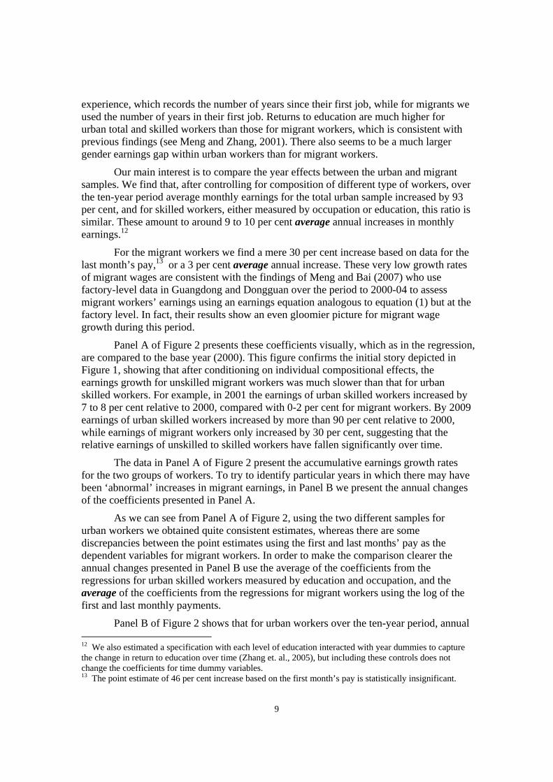
Our main interest is to compare the year effects between the urban and migrant samples. We find that, after controlling for composition of different type of workers, over the ten-year period average monthly earnings for the total urban sample increased by 93 per cent, and for skilled workers, either measured by occupation or education, this ratio is similar. These amount to around 9 to 10 per cent average annual increases in monthly earnings.12

For the migrant workers we find a mere 30 per cent increase based on data for the last month’s pay,13 or a 3 per cent average annual increase. These very low growth rates of migrant wages are consistent with the findings of Meng and Bai (2007) who use factory-level data in Guangdong and Dongguan over the period to 2000-04 to assess migrant workers’ earnings using an earnings equation analogous to equation (1) but at the factory level. In fact, their results show an even gloomier picture for migrant wage growth during this period.

Panel A of Figure 2 presents these coefficients visually, which as in the regression, are compared to the base year (2000). This figure confirms the initial story depicted in Figure 1, showing that after conditioning on individual compositional effects, the earnings growth for unskilled migrant workers was much slower than that for urban skilled workers. For example, in 2001 the earnings of urban skilled workers increased by 7 to 8 per cent relative to 2000, compared with 0-2 per cent for migrant workers. By 2009 earnings of urban skilled workers increased by more than 90 per cent relative to 2000, while earnings of migrant workers only increased by 30 per cent, suggesting that the relative earnings of unskilled to skilled workers have fallen significantly over time.

The data in Panel A of Figure 2 present the accumulative earnings growth rates for the two groups of workers. To try to identify particular years in which there may have been ‘abnormal’ increases in migrant earnings, in Panel B we present the annual changes of the coefficients presented in Panel A.

As we can see from Panel A of Figure 2, using the two different samples for urban workers we obtained quite consistent estimates, whereas there are some discrepancies between the point estimates using the first and last months’ pay as the dependent variables for migrant workers. In order to make the comparison clearer the annual changes presented in Panel B use the average of the coefficients from the regressions for urban skilled workers measured by education and occupation, and the average of the coefficients from the regressions for migrant workers using the log of the first and last monthly payments.

Panel B of Figure 2 shows that for urban workers over the ten-year period, annual 12 We also estimated a specification with each level of education interacted with year dummies to capture the change in return to education over time (Zhang et. al., 2005), but including these controls does not change the coefficients for time dummy variables. 13 The point estimate of 46 per cent increase based on the first month’s pay is statistically insignificant.

10

earnings growth hovered around 10 per cent per year. There are some significant ups and downs in these annual changes at the end of the period, but the general trend and rate of change in all other years is virtually constant.

For migrant workers between the years 2000 and 2002 there is almost no increase in earnings relative to that of the base year (with the increment of 2 per cent between 2000 and 2001 being offset by the 2 per cent reduction between 2001 and 2002). Between 2002 and 2004 there is a slight increase in earnings, with relatively strong growth of seven per cent between 2002 and 2003 (resulting largely from the decrease in earnings in 2002). The annual growth rate dropped to less than 2 per cent between 2003 and 2004, and then had two years of continuous growth through to 2006.

The increase between 2005 and 2006 may be considered as being close to ‘abnormal’ growth in that it is the first (and only) time that the annual earnings growth of migrant workers almost equalled that for urban workers. The next notable increase in earnings for migrant workers occurred in 2008 in which a 9.5 percent increase is observed. However, during the same period, the annual earnings growth for urban workers reached 17 per cent – coinciding with the annual CPI reaching a 10-year high of 6 per cent in 2008, while the producer price index (PPI) for farm products reached 14 per cent. If anything, this was a period of abnormal earnings growth for urban workers, but not for migrant workers.14

The above comparisons of annual increases in skilled urban and unskilled migrant earnings suggest that, apart from the period between 2005 and 2006, there were no abnormal earnings increases for migrant workers. In fact, it is clear from Panel A in Figure 2 that over the past ten years the earnings gap between migrant and urban workers has risen significantly as a result of the much faster increase in earnings for urban workers than for migrant workers. If we believe that the annual increase in the coefficients for the year dummies for urban workers is partly explained by rising living costs over time and partly explained by other (unexplained) demand and supply factors, it is quite likely that the increase in earnings for migrant workers may in fact not have been enough to offset the increase in living costs in cities. That is, the real income of migrant workers may have not increased at all. This observed reduction in the relative earnings of unskilled migrant workers is not consistent with a shortage of migrant labour supply.

The above comments not withstanding, the observed earnings increase for migrants between 2005 and 2006 that is almost equal to the increase for urban workers deserves further thought. Our time series data reveals that this increase for migrant workers’ earnings was not sustained beyond 2006, which in itself suggests that earlier papers citing higher wages as evidence of the arrival of the turning point may have been premature. In addition, it is insightful to consider some of the factors that may have generated this ‘almost abnormal’ migrant wage increase in this period.

First, there was a significant boost to FDI following the abolishment of American textile restrictions in 2004 (one of the WTO accession agreements). This significantly increased the demand for unskilled migrant labour with the effect taking place after 2004 and possibly peaking in 2006. 14 For more on the impact of the global financial crisis on rural migrants in China, see Kong et al. (2010).

11

Second, a number of the government’s new policy initiatives to promote a ‘harmonious’ society were introduced from 2004 onwards. These included the abolition of the agriculture tax, direct price subsidies to agricultural produce, and an increase in urban minimum wages. As shown in Figure 3, the first two initiatives raised rural per capita income, providing incentives for rural workers to stay at home rather than migrate. While these policies undoubtedly reduced the supply of migrant labour in these years, this does not amount to an exhaustion of rural surplus labour, given that the removal of either of these policies would see migrant numbers on the rise again. The increase in the urban minimum wage can be seen clearly in Figure 4 for Dongguan and Guangzhou cities – an example of a policy that would have driven up migrant earnings in these years without implying anything about the stock of rural surplus labour per se.

Finally, the special demographic structure of China also contributed to the temporary reduction of labour supply for some key migrant age cohorts. Figure 5 uses all individuals who have agricultural hukou from a 20 per cent sample of the one per cent population survey in 2005 to construct a rural population pyramid. The figure shows two clear troughs in the pyramid, one for 44 to 46 year olds and the other for 19 to 29 years old (between the two red bars in Figure 5). The first trough is the result of the 1959-1961 famine, and the second one is the echo effect of this famine in combination with the effect of the introduction of the one-child policy in the early 1980s. The second trough is particularly relevant to our search for the explanation of the almost abnormal increase in migrant earnings between 2005 and 2006. Due to China’s unique institutional settings, to be discussed in the next section, migrants are heavily concentrated in the 20-30 year age group. And in 2005-2006, the second trough falls exactly in those age groups, suggesting a temporary reduction in the pool of migrants but not a drying up of the migrant labour supply altogether.

In sum, changes in the relative earnings of unskilled migrant workers and skilled urban workers indicate that the growth of migrant earnings during the period 2000 to 2009 has been largely offset if not outweighed by increases in living costs in cities, suggesting that the real wages of migrant workers may have not increased at all. This finding is not consistent with claims of an exhausted rural labour supply, which, according to the theory, would result in rising real migrant wages. While a range of factors may have contributed to the increase in migrant earnings between 2005 and 2006, none of these factors indicate a continuous tightening of the migrant labour market. The next two sections confirm that the potential migrant labour supply is nowhere near reaching the limit.

4. Has rural China run out of surplus labour? Every developed economy has experienced the process through which the labour force moves from the less productive agricultural sector to the more productive industrial (and usually urban) sector. Japan, for example, saw its share of the labour force employed in agriculture fall from over 50 per cent in the 1920s to between 24-29 per cent during the 1960s – the period identified by Minami (1968) as Japan’s turning point. Figure 6 presents the proportion of the total labour force working in agriculture for a group of developed countries. The highest proportion among this group of 19 countries is 7 per cent in New Zealand. According to aggregated NBS data, 45 per cent of China’s labour

12

force was employed in the primary sector in 2005, although the one per cent population survey data places this much higher at 61 per cent.

The Rural Household Survey (RHS) of the RUMiCI survey data defines those who work in agriculture for nine or more months in a given year as having an agricultural job. According to this definition, in 2008 the proportions of the rural labour force working in agricultural jobs, rural non-agricultural jobs, or migrated were 49.2, 29.5 and 21.5 per cent respectively. Of those working in the rural non-agricultural sector, around 50 per cent were employed in nearby rural areas or county towns as production workers in the manufacturing and construction sectors, while the rest were scattered in trade, service and self-employment jobs. According to Au and Henderson (2006), a large fraction of existing Chinese cities are undersized, limiting the extent of urban agglomeration benefits. This is even more likely to be the case for non-agricultural sectors in rural areas and county towns and suggests that, in the future, many of these rural non-agricultural workers will move to cities.

Currently only a little over 20 per cent of China’s total rural labour force migrates to cities. Figure 7 presents the age and gender distribution of the migrated labour force for 2008. The figure shows that male migration rates peak at age 24, at which point 60 per cent of the labour force had migrated. For female workers, though, the migration rate peaks much earlier at age 21 with just over 50 per cent of this age migrating. Beyond these ages, migration rates drops dramatically. For example, between the ages of 24 and 30 there is a 15 percentage point drop for men, while for women between the ages of 21 and 26 there is a 15 percentage point drop. By the age of 35 only 20 per cent of women and 33 per cent of men are still migrated. This distribution has changed very little since large-scale migration started in the late 1990s. What this shows is that there is a significant churning of migrants going on, with migrants leaving for the cities in their late teens and returning home as early as their mid twenties. Section 5 considers the impact of this churning effect on low migration rates and the consequent stock of rural migrant labour in more detail.

A question that comes to mind is whether those members of the rural labour force who do not migrate are fully employed and earning comparable wages as those who migrate since this would provide another indication of the end of surplus labour. The RUMiCI RHS 2009 collected additional detailed information about the number of days individuals worked in agricultural and rural non-agricultural jobs. Table 2 presents the average number of days that rural workers who have not migrated worked in each of the sectors. Individuals who identified themselves as rural non-agricultural workers worked 244 days in off-farm jobs and 38 days in farming jobs. If we consider 300 days of work as a full time job, this group (comprising 29 per cent of the total rural labour force) seem not to be underemployed. However, individuals who identified themselves as agricultural workers worked an average of 154 days in the agricultural sector and 3.4 days in rural off-farm jobs. This means that 50 per cent of the agricultural labour force only work part time. In other words, underemployment in the agricultural sector is extraordinarily high.

The issue of whether rural workers who did not migrate earned wages comparable to their migrant counterparts is slightly more complicated. This is because rural agricultural workers have no observable earnings. As a proxy for rural agriculture earnings we use household income per labourer from households that have neither rural

13

off-farm workers nor migrants.15 According to this measure, in 2008 and 2009 respectively, migrants on average earned 61 per cent and 43 per cent higher monthly earnings than those in rural farming jobs and 19 per cent and 12 per cent more than those in rural non-farming jobs. These simple averages, however, do not control for labour quality differentials. To do so, we estimate a log monthly earnings equation controlling for age and its squared term, education, gender, and regional indicators. The two dummy variables of rural farming and off-farm jobs are compared to the omitted category of migrants. The results are reported in Table 3. We find that controlling for labour quality, the real earnings differentials between migrants and farm workers in 2008 and 2009 respectively were 53 and 35 per cent; while compared with off-farm workers, migrant earnings were 27 and 24 per cent higher.

The evidence above shows that there are still abundant workers who are under-employed and earning very low incomes; that migration rates are extremely low with significant churning; and that there are still significant migrant-rural wage differentials.16 The next obvious question is why wouldn’t more of these rural workers migrate to urban areas in order to access those higher earnings, as economic theory predicts? Put another way, is the pool of potential migrants really close to reaching exhaustion, or are there plenty more who are willing and able to migrate but choosing not to? The answer to this question provides further support for the ‘not yet’ camp in the turning point debate.

In particular, there are many impediments to rural-urban migration in China, including temporary rather than permanent working ‘visas’ in cities, and limited access to the social benefits available to their urban counterparts – including health facilities and pension provision, the lack of a safety net and their children not having the same access to schools as their urban peers. As a result, rural-urban migration in China has proceeded under a ‘guest worker’ system, whereby migrants in general do not move to cities with their families. Rather, they move to cities to work when they are young and unmarried and return to their rural homes when they need to form families. By and large, individuals with family responsibilities do not migrate.

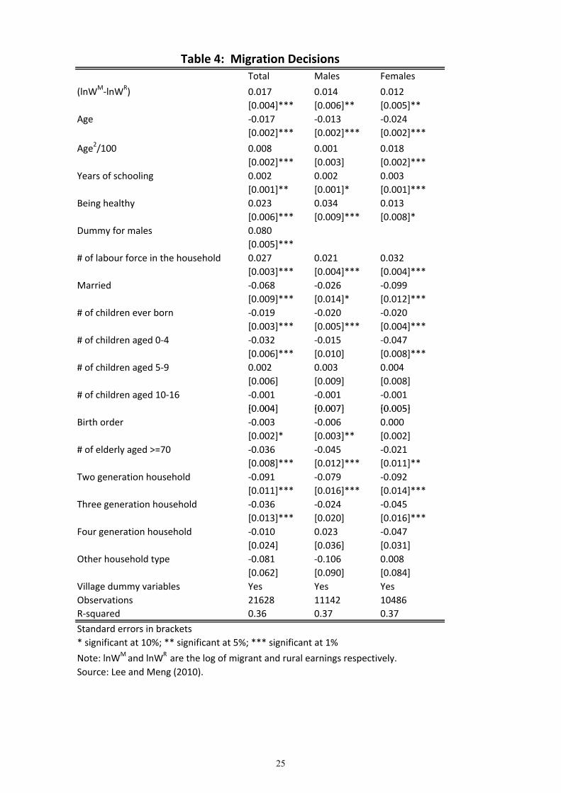
Using the RUMiCI RHS 2008, Lee and Meng (2010) examine the determinants of rural-urban migration using a linear probability model to estimate the determinants of migration and how each of these impact on each individual’s probability of migration. Table 4 reproduces their regression results for convenience, with the relevant findings summarised here.

As expected, the wage differential between urban and rural income is positively related to the probability of migration (i.e., the migration rate) for both men and women. 15  Note that the earnings of migrated individuals are reported by family members. These are likely to be under-reported as many people may not reveal their true earnings to their family, which will result in under-estimates of migrant earnings. Also note that, some migrant families have no information on their migrated members’ earnings, hence 10.7 and 7.7 per cent of the sample migrants in 2008 and 2009 are not included in this comparison due to missing values. It is not obvious whether the impact of these missing values will result in under- or over-estimates of migrant earnings.

16  Our data for 2009 shows a very similar pattern, with migration rates falling even lower as a result of the Global Financial Crisis.

14

Of more interest here is how China’s special institutional restrictions impact on individuals’ migration decisions. For example, due to the difficulty in accessing social services and social welfare, migrants often leave their family behind in the rural village while they go to the cities to earn money. Consequently, women (and married women in particular) and people with more family responsibilities are less likely to migrate. Fertility rates are negatively related to migration and the magnitude of the effect is similar for men and women. However, every additional child aged 0-4 years reduces a woman's migration probability by 5 per cent over and above the effect that the total number of children has on the probability of migration. This downward effect on women’s migration is nearly four times that of a one per cent change in the wage differential, an effect that does not hold for men. Another interesting finding concerns the age structure within households: relative to a single generation families, individuals from two-generation households have the lowest probability of migrating. Once again this may reflect childcare responsibility, since households with more than two generations presumably have grandparents who can look after the children when parents move to cities to work.

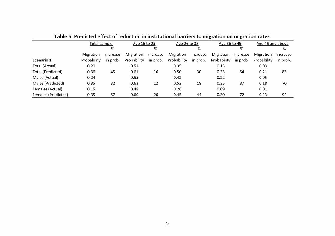
These results indicate that many of variables affecting individuals’ migration decisions may be policy induced. Lee and Meng (2010) conduct an exercise in which they assume that the policy on migrants’ access to social welfare is changed such that there is no effect of marriage status, presence of young children and elderly, and difference in household types on the migration decision. Using the results from their analysis presented in Table 4, they predict each individual’s migration probability assuming the impact of these family-related variables—marriage, number and age of children, number of elderly in the household, and whether the household is a two, three or four generation household—to be zero, which they interpret as being equivalent to removing all barriers to social services – or, in other words, to removing institutional barriers to migration.17

We reproduce their projection results in Table 5, where the actual and predicted probabilities for the total sample and by gender and age groups are presented. For the total sample, the actual probability of migration is 0.20: that is, one in five of the rural workforce had already migrated in 2008. Reducing the effect of the above family-related variables to zero the predicted probability of migration increases to 0.36 per cent, a 45 per cent increase. The effect is much stronger for females than for males (with a 57 per cent increase in migration probability compared with 32 per cent increase in migration probability), as expected given the distribution of family responsibilities within households. Among the four age groups, the older the group the greater the percentage increase in migration probability, because the older individuals become the more family responsibilities they have.18

17 This is a very strong assumption, which gives an upper bound increase in migration probability stemming from institutional reforms. They present an alternative scenario as well, which is less restrictive. See Lee and Meng (2010) for details on both. 18 Note that the model has a specific quadratic age effect built in and that the labour force for all the workers excludes those who are still at school. These are reasons why the predicted age-specific rates for the 16 year olds are very high and that the age effect is almost linearly negative (as can be seen clearly in the next section).

15

These projections indicate that there is the potential for a huge increase in the proportion of the labour force that could migrate if institutional barriers to migration were to be removed. This adds more weight to the evidence presented in this section, which in combination provides no reason to think that China has run out of surplus labour yet.

5. Effect of reduced churning: projections of rural labour supply through to 2020 In this section we investigate the question: by how much would the migrant supply stock increase if there was reduced churning in the migrant population? To address this question we conduct two thought experiments. First, we look at the effect of the increased length of stay on the stock of migrants in cities. Assume that currently there are 150 million rural migrants working in cities and on average they stay in cities for six years. If policy changes in cities increased the average length of stay by one year to seven years and assuming that the inflow/outflow does not change, the stock of total migrants would increase by (150)/(6)=25 million, or almost 17 per cent. If we assume that the average length of stay doubles to 12 years, the stock of total migrants will double. This indicates that a reduction in churning has an extremely important impact on increasing the migrant stock and that the government policy can do a great deal in easing migrant supply “shortage”.

The second thought experiment we conduct is to use the one per cent population survey of 2005 as the base year to project the rural migrant labour supply through to 2020 based on two alternative assumptions about how migrant rates change over time. As we have gender- and age-specific migration and employment rates, we use the following formula applied separately to female and male migrant workers and then add them together for the total migrant workforce. The total number of (male or female) rural migrant workers in 2005 can be expressed as:

RMx2005 = Px * Mx * Ex (3)

where 2005xRM is the total number of (male or female) rural migrant workers aged x in

2005. R xP is the gender-specific total population in 2005, xM and xE are the migration and employment rates for x year olds. We begin with the year 2005 so that we can utilise the 20 per cent sample of the 1 per cent population survey in 2005.19 Age- and gender-specific employment rates are also taken from this survey. The migration rates are based on the RUMiCI Rural Household Survey for 2008.20 Note that 0-15 year olds and over 65 year olds are assumed to have zero employment rates, and hence their migration rates are irrelevant, as they will not contribute to the labour supply, wherever they are. Summing across ages 16 to 65 gives us the total stock of (female or male) rural migrant

19 To generate national population estimates we multiply the sample populations by 500. 20  Clearly it would be more accurate to use migration rates for 2005 but we decided not to do so for two reasons. First, the 2005 population survey data do not have information on migration based on the same definition as that used in the RUMiCI survey data. This compatibility is necessary because we are going to use the estimation results presented in Table 4 using 2008 RUMiCI data as the base year for our projection. We therefore sacrifice some accuracy in the 2005-07 projections in order to maintain consistency across projections. Second, the migration rates for the gender and age specific group is closer to the current situation than those obtained from the 2005 population survey.

16

workers in 2005, on which all subsequent projections are based. Table 6 presents the data used in these calculations for a sample of age groups.

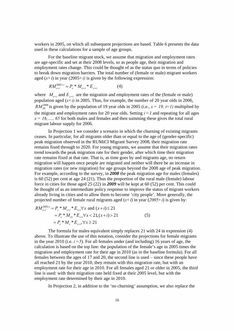
For the baseline migrant stock, we assume that migration and employment rates are age-specific and set at their 2008 levels, so as people age, their migration and employment rates change. This could be thought of as the status quo in terms of policies to break down migration barriers. The total number of (female or male) migrant workers aged (x+i) in year (2005+i) is given by the following expression:

RMx + i2005+ i = Px * Mx + i * Ex + i (4)

where Mx + i and Ex + i are the migration and employment rates of the (female or male) population aged (x+i) in 2005. Thus, for example, the number of 20 year olds in 2006,

200620RM is given by the population of 19 year olds in 2005 (i.e., x = 19, i=1) multiplied by

the migrant and employment rates for 20 year olds. Setting i =1 and repeating for all ages x = 16,…., 65 for both males and females and then summing these gives the total rural migrant labour supply for 2006.

In Projection 1 we consider a scenario in which the churning of existing migrants ceases. In particular, for all migrants older than or equal to the age of (gender-specific) peak migration observed in the RUMiCI Migrant Survey 2008, their migration rate remains fixed through to 2020. For young migrants, we assume that their migration rates trend towards the peak migration rate for their gender, after which time their migration rate remains fixed at that rate. That is, as time goes by and migrants age, no return migration will happen once people are migrated and neither will there be an increase in migration rates (or new migration) for age groups beyond the 2008 age of peak migration. For example, according to the survey, in 2008 the peak migration age for males (females) is 60 (52) per cent at age 24 (21). Thus the proportion of the rural male (female) labour force in cities for those aged 25 (22) in 2009 will be kept at 60 (52) per cent. This could be thought of as an intermediate policy response to improve the status of migrant workers already living in cities and to allow them to become ‘city people’. More generally, the projected number of female rural migrants aged (x+i) in year (2005+i) is given by:

RM x+i2005+i = Px * M x+i * Ex+i∀x and (x + i) ≤ 21

= Px * M21 * Ex+i∀x < 21,(x + i) > 21 = Px * M x * Ex+i,∀x ≥ 21

(5)

The formula for males equivalent simply replaces 21 with 24 in expression (4) above. To illustrate the use of this notation, consider the projections for female migrants in the year 2010 (i.e. i =5). For all females under (and including) 16 years of age, the calculation is based on the top line: the population of the female’s age in 2005 times the migration and employment rate for their age in 2010 (as in the baseline formula). For all females between the ages of 17 and 20, the second line is used – since these people have all reached 21 by the year 2010, they remain with this migration rate, but with an employment rate for their age in 2010. For all females aged 21 or older in 2005, the third line is used: with their migration rate held fixed at their 2005 level, but with the employment rate determined by their age in 2010.

In Projection 2, in addition to the ‘no churning’ assumption, we also replace the

17

baseline observed migration rates for each gender-age with the higher migration rates predicted in Lee and Meng (2010) in response to the elimination of all migration barriers.

Figure 8 presents the proportion of the rural labour force migrated in 2008 and 2020 for Projections 1 and 2 respectively. These essentially illustrate the migration rate assumptions underpinning our alternative projections, and highlight changes in the age- and gender distributions of the migrant workforce compared with the baseline distributions, which remain fixed through time at the rates illustrated in Figure 7.

Figure 9 and Table 7 summarise the changes in the stock of migrant labour for the two projections relative to the baseline. Under Projection 1, by 2020 the stock of migrants will increase by 106 million, 80 per cent higher than the baseline figure for the same year; while if we add the additional assumption of the relaxation on institutional barriers to entry, the total stock of migrants in 2020 will be 140 per cent higher than the baseline projection for the same year. While these scenarios are clearly hypothetical, the results still illustrate the intended point: policies to reduce institutional barriers to rural-urban migration and to stop migrant churning could substantially increase the stock of rural migrants into urban areas in the future. Were such policies to have been implemented earlier, it is quite likely that the observed labour shortages in southern coastal China may not have materialised, nor the observed rise in nominal wages that some scholars have attributed to these shortages.

6. Conclusions Researchers can clearly get the timing of the turning point wrong. Minami’s (1968) paper contradicted Fei and Ranis’s (1964) thesis that Japan had reached its turning point by 1920, with Minami’s claim that it did not in fact occur until the 1960s later becoming the widely accepted view. That both Ranis (2004) and Minami (and Ma, 2010) remain engaged in the turning point literature more than half a century since their first contributions illustrates the depth, breadth and contentious nature of the issues involved. This paper did not set out to pinpoint the precise year in which China is expected to reach its turning point in economic development. Instead, it aimed to contribute to the heated debate surrounding the question of whether or not that turning point has already arrived. The bulk of evidence presented above places us firmly on the side of those people arguing that it has not.

We first used the RUMiCI Migrant Survey and UHIES data to compare the wages of urban and migrant unskilled workers, demonstrating that once other factors were controlled for, the real wages of migrant workers may not have increased at all during the period 2000 to 2009. This finding is inconsistent with claims of an exhausted migrant labour supply, which according to the theory would result in rising real migrant wages. While there was some evidence of what might just be considered ‘abnormal’ wage growth between 2005 and 2006, we identified a number of factors that may have contributed to this. These included the introduction of policies that raised rural incomes and minimum wages in urban areas, alongside some peculiarities in China’s population pyramid, rather than the end of rural surplus labour per se.

Turning to the rural workforce, and drawing on the RUMiCI Rural Household Survey, we provided a range of evidence to demonstrate that by 2008 there was still an

18

abundance of rural workers who appeared to be under-employed with earnings well below their migrant counterparts. This, combined with evidence of low migration rates and significant ‘churning’ – migrants returning back to their villages from their early 20s onwards – immediately raised the question of why more rural workers are not migrating to urban areas, which in turn would clearly increase the rural migrant stock there. The immediate answer to this concerns the well-known continuation of a range of institutional barriers to migration, which impinge on the migration decisions of families in a range of ways. Rather than indicating an exhausted pool of migrant workers, our study indicates that if the average number of years of migration increased by just four years, the stock of migrants could more than double. We also provided projections through to 2020 assuming that policy changes would allow existing migrant cohorts to stay in the cities. By further eliminating all institutional barriers, the number of migrants could be more than doubled by 2020.

A deep understanding of the sources of wage growth in China and how that wage growth is distributed across the country is critical for the future welfare of Chinese workers. If, for example, rising urban wages are taken to signal an end of surplus labour but are instead due to migration barriers and labour market segmentation, the result could be a premature industrial restructuring towards more capital- and technology-intensive sectors of the economy in combination with the movement of labour-intensive industries offshore – a move that is already happening because of exactly this perception according to Brautigam (2009). This could effectively exclude a substantial number of Chinese workers from joining the industrial sectors of the economy in the future. As argued by Solinger (2001), social instability among these ‘disenfranchised’ workers could in turn pose one of the biggest threats to the legitimacy and stability and economic performance in China. The turning point issue is therefore most worthy of further research.

19

References Appleton, Simon, John Knight, Lina Song and Qingjie Xia, (2004), “Contrasting

paradigms: segmentation and competitiveness in the formation of the Chinese labour market”, Journal of Chinese Economic and Business Studies Vol 2(3):185-205.

Brautigam, Deborah (2009), The Dragon’s Gift: The real story of China in Africa, Oxford University Press, Oxford.

Brooks, Ray and Ran Tao (2003), “China’s labour market performance and challenges”, IMF Working Paper WP/03/210

Cai, Fang (2007a) "Lewsian Turning Point during China's Economic Growth" (Table 6-3), in Cai Fang and Du Yang (eds.) Green Book of Population and Labor: Lewisian Turning Point and Its Policy Challenges, (in Chinese) Social Science Academic Press (China), Beijing.

Cai, Fang (2007b) “Labour market development and rural/urban population growth”, Institute of Population and Labour Economics, Chinese Academy of Social Sciences, presentation in May 2007.

Cai, Fang (2010), “Demographic transition, demographic dividend, and Lewis turning point in China”, China Economic Journal, Vol. 3(2): 107-19.

Cai, Fang and Dewen Wang (2006), “Employment growth, labour scarcity and the nature of China’s trade expansion” in Garnaut, Ross and Ligang Song (eds) The Turning Point in China’s Economic Development, ANU E-press and Asia-Pacific Press.

Cai, Fang and Wang, Meiyan (2010) “Urbanisation with Chinese Characteristics”, Chapter in Garnaut, Ross, Jane Golley and Ligang Song (editors) China: The Next Twenty Years of Reform and Development, ANU E Press and Social Sciences Academic Press (China).

Cai, F. and Wang, M., 2007a, Growth and structural changes in employment in transitional China, unpublished manuscript, Beijing: Inistitute of Labour and Population Economics, CASS.

Cai, F. and Wang, M., 2007b, Labor cost increase and growth pattern in transition, unpublished manuscript, Beijing: Inistitute of Labour and Population Economics, CASS.

Chen, Yi, Démurger, Sylvie and Martin Fournier (2007), “The evolution of gender earnings gaps and discrimination in Urban China, 1988-95, Developing Economies 45(1): 97-121

Du, Y. and Wang, Meiyan (2010), “A discussion on potential bias and implications of Lewisian turning point’, China Economic Journal, Vol. 3(2): 121-36.

Démurger, Sylvie, Marc Gurgand, Li Shi and Yue Ximing (2009), “Migrants as second-class workers in urban China? A decomposition analysis”, Journal of Comparative Economics 37: 610-28.

20

Démurger, Sylvie, Martin Fournier, Li Shi and Wei Zhong (2007), “Economic liberalisation with rising segmentation in China’s urban labour market”, Asian Economic Papers 5(3): 58-101.

Fei, J.C.H. and G. Ranis (1964), Development of the Labour Surplus Economy: Theory and Policy, Irwin, Illinois.

Garnaut, Ross and Yiping Huang (2006), “Continued rapid growth and the turning point in China’s economic development” in Garnaut, Ross and Ligang Song (eds) The Turning Point in China’s Economic Development, ANU E-press and Asia-Pacific Press.

Garnaut, Ross (2010), “Macroeconomic implications of the turning point”, China Economic Journal, Vol. 3(2): 181-90.

Gong, X., Kong, S. T., Li, S., and Meng, X., 2008, “Rural-urban migrants: a driving force for growth”, in Ross Garnaut, Ligang Song and Wing Thye Woo (eds) China’s Dilemma, Canberra: Asia Pacific Press.

Islam, Nazrul and Kazuhiko Yokota, 2008 “Lewis Growth Model and China’s Industrialization”, Asian Economic Journal 22(4):359-96.

Knight, John, Lina Song and Jia Huaibin (1999), Chinese Rural Migrants in Urban Enterprises: Three perspectives”, Journal of Development Studies 35 (3):73-104

Knight, John, Quheng Deng and Shi Li (2010), “The puzzle of migrant labour shortage and the rural labour surplus in China”, The University of Oxford, DoE Working Paper Series No. 494.

Kong, Sherry Tao, Xin Meng, Dandan Zhang (2010), “The Global Financial Crisis and Rural-Urban Migration”, Chapter in Garnaut, Ross, Jane Golley and Ligang Song (editors) China: The Next Twenty Years of Reform and Development, ANU E Press and Social Sciences Academic Press (China).

Lee, L., and Meng, X., 2010, “Why Don’t More Chinese Migrate from the Countryside? Institutional Constraints and the Migration Decision” in X. Meng and C. Manning, with S. Li, and T.Effendi (eds) The Great Migration: Rural-Urban Migration in China and Indonesia, Edward Elgar Publishing Ltd.

Lewis, W.A. (1954) “Economic Development with Unlimited Supplies of Labour”, The Manchester School, Vol 22 (2): 139-91.

Lewis, A., 1958, Unlimited supply of labour: further notes, The Manchester School Economic and Social Studies, 26(1), pp.1-32.

Meng, Xin and Junsen Zhang (2001), “The two-tier labour market in urban China: occupational segregation and wage differentials between urban residents and rural migrants in Shanghai”, Journal of Comparative Economics 29:485-504.

Meng, Xin and Nansheng Bai (2007), “How much have the wages of unskilled workers in China increased? Data from seven factories in Guangdong” in Garnaut, Ross and Ligang Song (eds) China: Linking markets for growth, Asia-Pacific Press, Canberra and Social Sciences Academic Press, Beijing.

21

Minami, Ryoshin (1968), “The Turning point in the Japanese economy”, The Quarterly Journal of Economics, Vol. 82 (3): 380-402.

Minami, Ryoshin and Xinxin Ma (2010), “The Turning point of Chinese economy: compared with Japanese experience”, China Economic Journal, Vol. 3(2): 163-80.

Ranis, Gustav (2004), “Arthur Lewis’s contribution to Development Thinking and Policy”, Special issue of The Manchester School, Vol 72 (6):712-23.

Ranis, G. and J.C.H. Fei (1961), “A Theory of Economic Development”, American Economic Review Vol. LI:533-65.

Solinger, Dorothy (2001), “Globalization and the paradox of participation: the Chinese case”, Global Governance 7: 176-96.

Tyers, Rod and Golley, Jane (2010) “China's growth to 2030: The roles of demographic change and financial reform”, Review of Development Economics 14(3): 592-610, translated into Chinese, in China Labour Economics, Vol. 4, No. 1: 3-30.

World Bank (2007), China Quarterly Update, September, World Bank Office, Beijing.

Yao, Yang and Ke Zhang (2010), “Has China passed the Lewis turning point? A structural estimation based on provincial data”, China Economic Journal, Vol. 3(2): 155-62.

Zhang, J., Zhao, Y. Park, A., and Song, X., 2005, “Economic returns to schooling in urban China, 1988 to 2001”, Journal of Comparative Economics, 33(4), pp.730-752.

Zhao and Wu (2007) “Special Report: Analysis of Wages of Rural-Urban Migrants”, in Cai Fang and Du Yang (eds.) Green Book of Population and Labor (2007) Lewisian Turning Point and Its Policy Challenges, (in Chinese) Social Science Academic Press (China), Beijing.

Total sampleSkilled by occupation

Skilled by education

Last month wage

First month wage

age 0.046*** 0.049*** 0.039*** 0.006 0.010***[0.001] [0.002] [0.002] [0.004] [0.004]

Age squared ‐0.001*** ‐0.001*** ‐0.000*** ‐0.0001 ‐0.0001[0.000] [0.000] [0.000] [0.000] [0.000]

Firm tenure/work experience 0.024*** 0.022*** 0.028*** 0.051***[0.000] [0.001] [0.001] [0.008]

(Firm tenure/work experience)2 ‐0.000*** ‐0.000*** ‐0.000*** ‐0.002***[0.000] [0.000] [0.000] [0.000]

University and above 0.930*** 0.728*** 0.587*** 0.435*** 0.497***[0.006] [0.012] [0.003] [0.115] [0.112]

3‐year college 0.658*** 0.475*** 0.309*** 0.355*** 0.263***[0.006] [0.012] [0.002] [0.051] [0.050]

Senior high/technical high school 0.353*** 0.242*** 0.256*** 0.173***[0.006] [0.012] [0.037] [0.038]

Junior high school 0.154*** 0.064*** 0.099*** 0.073**[0.006] [0.012] [0.035] [0.036]

Dummy for females ‐0.246*** ‐0.180*** ‐0.214*** ‐0.099*** ‐0.065***[0.002] [0.002] [0.002] [0.019] [0.019]

Year Dummies2001 0.075*** 0.079** 0.078** 0.010 0.037

[0.027] [0.036] [0.032] [0.044] [0.039]2002 0.165*** 0.194*** 0.170*** 0.005 0.004

[0.020] [0.026] [0.023] [0.045] [0.036]2003 0.254*** 0.290*** 0.261*** 0.080* 0.069**

[0.020] [0.026] [0.023] [0.043] [0.035]

 RUMiCI Data

Migrant workersUrban local workers

UHIES Data

Table 1: Earnings regressions for urban local workers and migrant workers, 2000‐2009

2004 0.351*** 0.383*** 0.354*** 0.106** 0.074**[0.020] [0.026] [0.023] [0.042] [0.035]

2005 0.464*** 0.495*** 0.470*** 0.143*** 0.135***[0.020] [0.026] [0.023] [0.041] [0.035]

2006 0.558*** 0.575*** 0.559*** 0.169*** 0.256***[0.020] [0.026] [0.023] [0.041] [0.036]

2007 0.691*** 0.687*** 0.687*** 0.274*** 0.256***[0.020] [0.026] [0.023] [0.041] [0.039]

2008 0.864*** 0.855*** 0.856*** 0.328*** 0.393***[0.020] [0.026] [0.023] [0.046] [0.055]

2009 0.934*** 0.916*** 0.925*** 0.291*** 0.470[0.019] [0.025] [0.023] [0.063] [0.309]

Province Yes Yes Yes Yes YesObservations 436162 231697 322546 3815 3393R‐squared 0.409 0.404 0.402 0.15 0.15

*** p<0.01, ** p<0.05, * p<0.1Standard errors in brackets

22

mean (days)Distribution: Freq. % Freq. %0‐99 days 3,620 35.6 153 3.2100‐149 days 1,123 11.1 520 10.7150‐199 days 1,331 13.1 574 11.8200‐249 days 1,554 15.3 806 16.6250‐299 days 913 9.0 753 15.5300‐365 days 1,616 15.9 2,053 42.3

Mean (days)

244

Table 2: Annual Days of Work for Rural (non‐migrant) Workforce

3.4 38

Rural Agricultural workers Rural non‐agricultural workersFarming working days Off‐farm work days

Off‐farm work days Farming working days

154

23

2008 2009Rural Farming job ‐0.526*** ‐0.349***

[0.017] [0.015]Rural Off‐farm job ‐0.273*** ‐0.235***

[0.015] [0.016]Age 0.059*** 0.059***

[0.003] [0.003]Age Squared ‐0.001*** ‐0.001***

[0.000] [0.000]Primary school 0.062* ‐0.016

[0.034] [0.033]Junor high school 0.102*** 0.053*

[0.033] [0.032]Senior high school 0.235*** 0.198***

[0.036] [0.034]Post secondary 0.150 0.122

[0.650] [0.366]Dummy for females ‐0.157*** ‐0.166***

[0.012] [0.011]Province Yes YesObservations 13819 14004R‐squared 0.192 0.159

*** p<0.01, ** p<0.05, * p<0.1Standard errors in brackets

Table 3: Real earnings differentials between rural workforce and migrants

Standard errors in brackets

24

Total Males Females

(lnWM‐lnWR) 0.017 0.014 0.012[0.004]*** [0.006]** [0.005]**

Age ‐0.017 ‐0.013 ‐0.024[0.002]*** [0.002]*** [0.002]***

Age2/100 0.008 0.001 0.018[0.002]*** [0.003] [0.002]***

Years of schooling 0.002 0.002 0.003[0.001]** [0.001]* [0.001]***

Being healthy 0.023 0.034 0.013[0.006]*** [0.009]*** [0.008]*

Dummy for males 0.080[0.005]***

# of labour force in the household 0.027 0.021 0.032[0.003]*** [0.004]*** [0.004]***

Married ‐0.068 ‐0.026 ‐0.099[0.009]*** [0.014]* [0.012]***

# of children ever born ‐0.019 ‐0.020 ‐0.020[0.003]*** [0.005]*** [0.004]***

# of children aged 0‐4 ‐0.032 ‐0.015 ‐0.047[0.006]*** [0.010] [0.008]***

# of children aged 5‐9 0.002 0.003 0.004[0.006] [0.009] [0.008]

# of children aged 10‐16 ‐0.001 ‐0.001 ‐0.001[0 004] [0 007] [0 005]

Table 4:  Migration Decisions 

[0.004] [0.007] [0.005]Birth order ‐0.003 ‐0.006 0.000

[0.002]* [0.003]** [0.002]# of elderly aged >=70 ‐0.036 ‐0.045 ‐0.021

[0.008]*** [0.012]*** [0.011]**Two generation household ‐0.091 ‐0.079 ‐0.092

[0.011]*** [0.016]*** [0.014]***Three generation household ‐0.036 ‐0.024 ‐0.045

[0.013]*** [0.020] [0.016]***Four generation household ‐0.010 0.023 ‐0.047

[0.024] [0.036] [0.031]Other household type ‐0.081 ‐0.106 0.008

[0.062] [0.090] [0.084]Village dummy variables Yes Yes YesObservations 21628 11142 10486R‐squared 0.36 0.37 0.37

Standard errors in brackets* significant at 10%; ** significant at 5%; *** significant at 1%

Note: lnWM and lnWR  are the log of migrant and rural earnings respectively.Source: Lee and Meng (2010).

25

Scenario 1Migration Probability

% increase in prob.

Migration Probability

% increase in prob.

Migration Probability

% increase in prob.

Migration Probability

% increase in prob.

Migration Probability

% increase in prob.

Total (Actual) 0.20 0.51 0.35 0.15 0.03Total (Predicted) 0.36 45 0.61 16 0.50 30 0.33 54 0.21 83Males (Actual) 0.24 0.55 0.42 0.22 0.05Males (Predicted) 0.35 32 0.63 12 0.52 18 0.35 37 0.18 70Females (Actual) 0.15 0.48 0.26 0.09 0.01Females (Predicted) 0.35 57 0.60 20 0.45 44 0.30 72 0.23 94

Table 5: Predicted effect of reduction in institutional barriers to migration on migration rates Total sample Age 16 to 25 Age 26 to 35 Age 36 to 45 Age 46 and above

26

Age in 2005 (x )Rural FemalePop. (P) 

Migration Rate (M) 

Employ. Rate (E) 

Rural FemaleMigrant Workers (P*M*E)

Rural MalePop. (P) 

Migration Rate (M) 

Employ. Rate (E) 

Rural MaleMigrant Workers  (P*M*E)

Total migrantworkers  

16 9,400,000 0.35 0.23 751,773 9,748,000 0.31 0.22 682,344 47,76317 8,399,500 0.48 0.41 1,678,197 8,448,000 0.40 0.38 1,277,200 193,09218 8,709,000 0.55 0.57 2,738,725 8,462,500 0.49 0.54 2,235,269 590,42019 7,145,500 0.54 0.68 2,650,640 6,786,000 0.49 0.66 2,213,056 721,72320 6,518,500 0.55 0.75 2,714,460 5,977,500 0.54 0.78 2,491,762 1,038,70930 6,995,500 0.31 0.82 1,783,536 6,820,000 0.51 0.97 3,351,683 1,647,18140 8,953,000 0.08 0.88 641,009 8,705,000 0.24 0.97 1,989,534 454,70950 6,696,500 0.01 0.79 73,168 6,873,500 0.06 0.95 402,741 23,59860 3,742,500 0.01 0.52 19,465 3,752,000 0.01 0.81 29,767 236

Total 332,387,000 0.17 45,861,665 429,515,000 0.26 77,533,696 123,395,361

Females Males

Table 6: Baseline Data for Rural Migrants, 2005

Note: Column One provides sample ages only, for space reasons. Population and worker totals are summed across all ages 0‐65 and 16‐65 respectively.

27

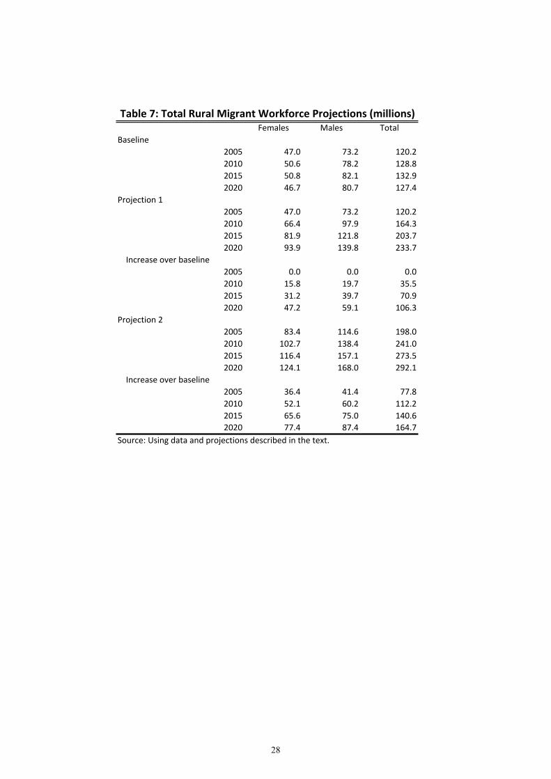
Females Males TotalBaseline

2005 47.0 73.2 120.22010 50.6 78.2 128.82015 50.8 82.1 132.92020 46.7 80.7 127.4

Projection 12005 47.0 73.2 120.22010 66.4 97.9 164.32015 81.9 121.8 203.72020 93.9 139.8 233.7

    Increase over baseline2005 0.0 0.0 0.02010 15.8 19.7 35.52015 31.2 39.7 70.92020 47.2 59.1 106.3

Projection 22005 83.4 114.6 198.02010 102.7 138.4 241.02015 116.4 157.1 273.52020 124.1 168.0 292.1

    Increase over baseline2005 36.4 41.4 77.82010 52.1 60.2 112.22015 65.6 75.0 140.62020 77.4 87.4 164.7

Source: Using data and projections described in the text.

Table 7: Total Rural Migrant Workforce Projections (millions)

28

 

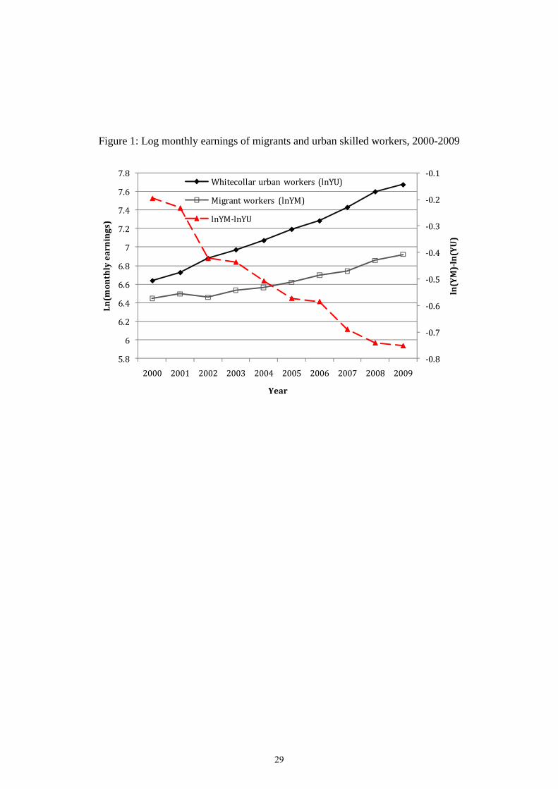
Figure 1: Log monthly earnings of migrants and urban skilled workers, 2000-2009

‐0.8

‐0.7

‐0.6

‐0.5

‐0.4

‐0.3

‐0.2

‐0.1

5.8

6

6.2

6.4

6.6

6.8

7

7.2

7.4

7.6

7.8

2000 2001 2002 2003 2004 2005 2006 2007 2008 2009

ln(YM)­ln(YU)

Ln(monthly earnings)

Year

Whitecollar urban workers (lnYU)

Migrant workers  (lnYM)

lnYM‐lnYU

 

29

 

Figure 2: Conditional earnings changes over time for urban and migrant workers, 2000‐2009 

Panel A: The estimated coefficients on year effects 

0

0.1

0.2

0.3

0.4

0.5

0.6

0.7

0.8

0.9

1

2001 2002 2003 2004 2005 2006 2007 2008 2009

Total urban

skilled urban (occ)

skilled urban (edu)

Migrant last month

Migrant first month

 

Panel B: The annual change of the estimated average year effects 

‐0.1

‐0.05

0

0.05

0.1

0.15

0.2

2001 2002 2003 2004 2005 2006 2007 2008 2009

Urban skilled workers

Migrant workers

 

  Sources: Author’s own estimation, see Table 2. 

 

30

Figure 3: Change in rural per capita income 

 Source: China Statistical Yearbook, NBS (2008) 

Figure 4: Change in minimum wage for Guangzhou and Dongguan 

 

 

 

 

 

 

 

 

 

 

 Sources: Guangdong provincial government web information in various years. 

0

100

200

300

400

500

600

700

800

900

1999 2000 2001 2002 2003 2004 2005 2006

Year

Mon

thly

min

imum

wag

e (Y

uan)

Guangzhou Dongguan

31

Figure 5: Rural Population Pyramid 

010

2030

4050

6070

8090

100

110

Age

20000 10000 0 10000 20000Population

Males Females

 

Source: 20 per cent sample of the 2005 one per cent population survey 

Figure 6: % of Labour Force Working in the Agricultural Sector—Developed Countries 

  

Source: CIA World Facebook.

32

Figure 7: Proportion of rural labour force migrated by gender and year 

0.2

.4.6

(mea

n) d

mig

20 30 40 50 60 70age

Male, 2008 Female, 2008

 

Source: RUMiCI Migrant Survey 2008 

33

Figure 8: Projected Changes in Migration Rates by 2020 

   

 

 

 

 

 

 

 

 

 

 

 

34

Figure 9. Projections of Total Rural Migrant Workforce through to 2020 

 

 

35