global well-posedness and non-linear stability of ...w3.impa.br/~cmateus/files/sbo-cpaa.pdf ·...
TRANSCRIPT

COMMUNICATIONS ON doi:10.3934/cpaa.2009.8.1PURE AND APPLIED ANALYSISVolume 8, Number 3, May 2009 pp. –
GLOBAL WELL-POSEDNESS AND NON-LINEAR STABILITY OFPERIODIC TRAVELING WAVES FOR A
SCHRODINGER-BENJAMIN-ONO SYSTEM
Jaime Angulo
IME-USP, Department of Mathematics
Rua do Matao 1010, Cidade Universitaria, CEP 05508-090, Sao Paulo, SP, Brazil.
Carlos Matheus
IMPA, Estrada Dona Castorina 110,CEP 22460-320 Rio de Janeiro, RJ, Brazil.
Didier Pilod
UFRJ, Institute of Mathematics, Federal University of Rio de Janeiro,
P.O. Box 68530, CEP: 21945-970, Rio de Janeiro, RJ, Brazil.
(Communicated by Gigliola Staffilani)
Abstract. The objective of this paper is two-fold: firstly, we develop a local
and global (in time) well-posedness theory for a system describing the motion
of two fluids with different densities under capillary-gravity waves in a deepwater flow (namely, a Schrodinger-Benjamin-Ono system) for low-regularity
initial data in both periodic and continuous cases; secondly, a family of newperiodic traveling waves for the Schrodinger-Benjamin-Ono system is given:
by fixing a minimal period we obtain, via the implicit function theorem, a
smooth branch of periodic solutions bifurcating a Jacobian elliptic functioncalled dnoidal, and, moreover, we prove that all these periodic traveling waves
are nonlinearly stable by perturbations with the same wavelength.
1. Introduction. In this paper we are interested in the study of the followingSchrodinger-Benjamin-Ono (SBO) system
iut + uxx = αvu,vt + γDvx = β(|u|2)x,
(1)
where u = u(t, x) is a complex-valued function, v = v(t, x) is a real-valued function,t ∈ R, x ∈ R or T, α, β and γ are real constants such that α 6= 0 and β 6= 0,and D∂x is a linear differential operator representing the dispersive term. HereD = H∂x where H denotes the Hilbert transform defined as
Hf(k) = −isgn(k)f(k),
where
sgn(k) = −1, k < 0,
1, k > 0.
2000 Mathematics Subject Classification. Primary: 35Q55, 35Q51; Secondary: 76B25, 76B15.
Key words and phrases. Nonlinear PDE, initial value problem, traveling wave solutions.The first author is partially supported by CNPq/Brazil.
1

2 J. ANGULO, C. MATHEUS AND D. PILOD
Note that from these definitions we have that D is a linear positive Fourier operatorwith symbol |k|. The system (1) was deduced by Funakoshi and Oikawa ([22]). Itdescribes the motion of two fluids with different densities under capillary-gravitywaves in a deep water flow. The short surface wave is usually described by aSchrodinger type equation and the long internal wave is described by some sort ofwave equation accompanied with a dispersive term (which is a Benjamin-Ono typeequation in this case). This system is also of interest in the sonic-Langmuir waveinteraction in plasma physics [30], in the capillary-gravity interaction wave [21], [27],and in the general theory of water wave interaction in a nonlinear medium [13], [14].We note that the Hilbert transform considered in [22] for describing system (1) isgiven as −H.
In studying an initial value problem, the first step is usually to investigate inwhich function space well-posedness occurs. In our case, smooth solutions of theSBO system (1) enjoy the following conserved quantities
G(u, v) ≡ Im
∫u(x)ux(x) dx +
α
2β
∫|v(x)|2 dx,
E(u, v) ≡∫|ux(x)|2 dx + α
∫v(x)|u(x)|2 dx− αγ
2β
∫|D1/2v(x)|2 dx,
H(u, v) ≡∫|u(x)|2 dx,
(2)
where D1/2 is the Fourier multiplier defined as D1/2v(k) = |k| 12 v(k). Therefore, thenatural spaces to study well-posedness are the Sobolev Hs-type spaces. Moreover,due to the scaling property of the SBO system (1) (see [9] Remark 2), we are led toinvestigate well-posedness in the spaces Hs ×Hs−1/2, s ∈ R.
In the continuous case Bekiranov, Ogawa, and Ponce [10] proved local well-posedness for initial data in Hs(R) × Hs− 1
2 (R) when |γ| 6= 1 and s ≥ 0. Thus,because of the conservation laws in (2), the solutions extend globally in time whens ≥ 1, in the case αγ
β < 0. Recently, Pecher [35] has shown local well-posedness in
Hs(R)×Hs− 12 (R) when |γ| = 1 and s > 0. He also used the Fourier restriction norm
method to extend the global well-posedness result when 1/3 < s < 1, always in thecase αγ
β < 0. Here, we improve the global well-posedness result till L2(R)×H− 12 (R)
in the case γ 6= 0 and |γ| 6= 1. Indeed, we refine the bilinear estimates of Bekiranov,
Ogawa, and Ponce [10] in Bourgain spaces X0,b1 × Y− 1
2 ,bγ with b, b1 < 1
2 (seeProposition 3.4). These estimates combined with the L2-conservation law allow usto show that the size of the time interval provided by the local well-posedness theorydepends only on the L2-norm of u0. It is worth while to point out that this schemeapplies for other dispersive systems. In fact Colliander, Holmer, and Tzirakis [19]already applied this method to Zakharov and Klein-Gordon-Schrodinger systems.They also announced the above result for the SBO system (see Remark 1.5 in[19]). However they allowed us to include it in this paper since there were notplanning to write it up anymore. Note that we also prove global well-posednessin Hs(R) × Hs− 1
2 (R) when s > 0 in the case γ 6= 0 and |γ| 6= 1. We take theopportunity to express our gratitude to Colliander, Holmer and Tzirakis for thefruitful interaction about the Schrodinger-Benjamin-Ono system.
In the periodic setting, there does not exist, as far as we know, any result aboutthe well-posedness of the SBO system (1). Bourgain [16] proved well-posedness forthe cubic nonlinear Schrodinger equation (NLS) (see (3)) in Hs(T) for s ≥ 0 using

SCHRODINGER-BENJAMIN-ONO SYSTEM 3
the Fourier transform restriction method. Unfortunately, this method does notapply directly for the Benjamin-Ono equation. Nevertheless, using an appropriateGauge transformation introduced by Tao [37], Molinet [33] proved well-posednessin L2(T). Here we apply Bourgain’s method for the SBO system to prove its localwell-posedness in Hs(T)×Hs− 1
2 (T) when s ≥ 1/2 in the case γ 6= 0, |γ| 6= 1. Themain tool is the new bilinear estimate stated in Proposition 3.11. Furthermore,by standard arguments based on the conservation laws, this leads to global well-posedness in the energy space H1(T)×H1/2(T) in the case αγ
β < 0. We also showthat our results are sharp in the sense that the bilinear estimates on these Bourgainspaces fail whenever s < 1/2 and |γ| 6= 1 or s ∈ R and |γ| = 1. In fact, we useDirichlet’s Theorem on rational approximation to locate certain plane waves whosenonlinear interactions behave badly in low regularity.
In the second part of this paper, we turn our attention to another importantaspect of dispersive nonlinear evolution equations: the traveling waves. The ex-istence of these solutions imply a balance between the effects of nonlinearity anddispersion. Depending on the specific boundary conditions on the wave’s shape,these special states of motion can arise as either solitary or periodic waves. Thestudy of this special steady waveform is essential for the explanation of many wavephenomena observed in practice: in surface water waves propagating in a canal, inpropagation of internal waves or in the interaction between long waves and shortwaves as in our case. In particular, some questions such as existence and stabilityof these traveling waves are very important in the understanding of the dynamic ofthe equation under investigation.
The solitary waves are in general a single crested, symmetric, localized travelingwaves, with sech-profiles (see Ono [34] and Benjamin [11] for the existence of solitarywaves of algebraic type or with a finite number of oscillations). The study ofthe nonlinear stability or instability of solitary waves has had a big developmentand refinement in recent years. The proofs have been simplified and sufficientconditions have been obtained to insure the stability to small localized perturbationsin the waveform. Those conditions have showed to be effective in a variety ofcircumstances, see for example [1], [2], [3], [12], [15], [26], [38].
The situation regarding to the study of periodic traveling waves is very different.The stability and the existence of explicit formulas of these progressive wave trainshave received comparatively little attention. Recently many research papers aboutthis issue have appeared for specify dispersive equations, such as the existence andstability of cnoidal waves for the Korteweg-de Vries equation [5] and the stabilityof dnoidal waves for the one-dimensional cubic nonlinear Schrodinger equation
iut + uxx + |u|2u = 0, (3)
where u = u(t, x) ∈ C and x, t ∈ R (Angulo [4], see also Angulo, and Linares [6]and Gallay, and Haragus [23], [24]).
In this paper we are also interested in giving a stability theory of periodic trav-eling waves solutions for the nonlinear dispersive system SBO (1). The periodictraveling waves solutions considered here will be of the general form
u(x, t) = eiωteic(x−ct)/2φ(x− ct),v(x, t) = ψ(x− ct),
(4)

4 J. ANGULO, C. MATHEUS AND D. PILOD
where φ, ψ : R→ R are smooth, L-periodic functions (with a prescribed period L),c > 0, ω ∈ R and we will suppose that there is a q ∈ N such that
4qπ/c = L.
So, by replacing these permanent waves form into (1) we obtain the pseudo-differentialsystem
φ′′ − σφ = α ψφγHψ′ − cψ = βφ2 + Aφ,ψ
(5)
where σ = ω− c2
4 and Aφ,ψ is an integration constant which we will set equal zero inour theory. Existence of analytic solutions of system (5) for γ 6= 0 is a difficult task.In the framework of traveling waves of type solitary waves, namely, the profiles φ, ψsatisfying φ(ξ), ψ(ξ) → 0 as |ξ| → ∞, it is well known the existence of solutions for(5) in the form
φ0,s(ξ) =√
2cσ
αβsech(
√σξ), ψ0,s(ξ) = −β
cφ2
0,s(ξ) (6)
when γ = 0, σ > 0, and αβ > 0. For γ 6= 0 a theory of even solutions of thesepermanent wave solutions has been established in [7] (see also [8]) by using theconcentration-compactness method.
For γ = 0 and σ > 2π2/L2 we prove (along the lines of Angulo [4] with regardto (3)) the existence of a smooth curve of even periodic traveling wave solutions for(5) with α = 1, β = 1/2; note that this restriction does not imply loss of generality.This construction is based on the dnoidal Jacobian elliptic function, namely,
φ0(ξ) = η1 dn( η1
2√
cξ; k
)
ψ0(ξ) = −η21
2cdn2
( η1
2√
cξ; k
),
(7)
where η1 and k are positive smooth functions depending of the parameter σ. Weobserve that the solution in (7) gives us “ in the limit ” the solitary waves solutions(6) when η1 →
√4cσ and k → 1−, because in this case the elliptic function dn
converges, uniformly on compacts sets, to the hyperbolic function sech.In the case of our main interest, γ 6= 0, the existence of periodic solutions is a
delicate issue. Our approach for the existence of these solutions uses the implicitfunction theorem together with the explicit formulas in (7) and a detailed study ofthe periodic eigenvalue problem associated to the Jacobian form of Lame’s equation
d2
dx2Ψ + [ρ− 6k2sn2(x; k)]Ψ = 0
Ψ(0) = Ψ(2K(k)), Ψ′(0) = Ψ′(2K(k)),(8)
where sn(·; k) is the Jacobi elliptic function of type snoidal and K = K(k) representsthe complete elliptic integral of the first kind and defined for k ∈ (0, 1) as
K(k) =∫ 1
0
dt√(1− t2)(1− k2t2)
.
So, by fixing a period L, and choosing c and ω such that σ ≡ ω − c2
4 satisfiesσ > 2π2/L2, we obtain a smooth branch γ ∈ (−δ, δ) → (φγ , ψγ) of periodic travelingwave solutions of (5) with a fundamental period L and bifurcating from (φ0, ψ0) in(7). Moreover, we obtain that for γ near zero φγ(x) > 0 for all x ∈ R and ψγ(x) < 0for γ < 0 and x ∈ R.

SCHRODINGER-BENJAMIN-ONO SYSTEM 5
Furthermore, concerning the non-linear stability of each point in this branch ofperiodic solutions, we extend the classical approach developed by Benjamin [12],Bona [15], and Weinstein [38] to the periodic case. In particular, using the con-servation laws (2), we prove that the solutions (φγ , ψγ) are stable in H1
per([0, L])×H
12per([0, L]) at least when γ is negative near zero. We use essentially the Benjamin,
Bona, and Weinstein’s stability ideas because it gives us an easy form of manipulat-ing with the required spectral conditions and the positivity property of the quantityd
dσ
∫φ2
γ(x)dx, which are basic information in our stability analysis.However, we do not use the abstract stability theory of Grillakis et al. [26] in our
approach basically because of the two circumstances above. We recall that Grillakiset al. theory in general requires a study of the Hessian for the function
d(c, ω) = L(eicξ/2φγ , ψγ) ≡ E(eicξ/2φγ , ψγ) + cG(eicξ/2φγ , ψγ) + ωH(eicξ/2φγ , ψγ)
with γ = γ(c, ω), and a specific spectrum information of the matrix linear operatorHc,ω = L′′(eicξ/2φγ , ψγ). In our case, these facts do not seem to be easily obtained.
So, for γ < 0 we reduce the required spectral information (see formula (100)) tothe study of the self-adjoint operator Lγ ,
Lγ = − d2
dξ2+ σ + αψγ − 2αβφγ K−1
γ φγ ,
where K−1γ is the inverse operator of Kγ = −γD + c. Hence we obtain via the
min-max principle that Lγ has a simple negative eigenvalue and zero is a simpleeigenvalue with eigenfunction d
dxφγ provide that γ is small enough.Finally, we close this introduction with the organization of this paper: in Section
2, we introduce some notations to be used throughout the whole article; in Section3, we prove the global well-posedness results in the periodic and continuous settingsvia some appropriate bilinear estimates; in Section 4, we show the existence ofperiodic traveling waves by the implicit function theorem; then, in Section 5, wederive the stability of these waves based on the ideas of Benjamin and Weinstein,that is, to manipulate the information from the spectral theory of certain self-adjointoperators and the positivity of some relevant quantities.
2. Notation. For any positive numbers a and b, the notation a . b means thatthere exists a positive constant θ such that a ≤ θb. Here, θ may depend only oncertain parameters related to the equation (1) such as γ, α, β. Also, we denotea ∼ b when, a . b and b . a.
For a ∈ R, we denote by a+ and a− a number slightly larger and smaller thana, respectively.
In the sequel, we fix ψ a smooth function supported on the interval [−2, 2] suchthat ψ(x) ≡ 1 for all |x| ≤ 1 and, for each T > 0, ψT (t) := ψ(t/T ).
Let L > 0. The inner product of two functions in L2([0, L]) is given by
< f, g >=∫ L
0
f(x)g(x)dx, ∀f, g ∈ L2([0, L]).
Now let P ′L be the set of periodic distributions of period L. For all s ∈ R we denoteby Hs
per([0, L]) = HsL(R) the set of all f in P ′L such that
‖f‖HsL
=
(L
+∞∑n=−∞
(1 + |n|2)s|f(n)|2) 1
2
< ∞,

6 J. ANGULO, C. MATHEUS AND D. PILOD
where (f(n))n∈Z denote the Fourier series of f (for further information see Iorio andIorio [29]). Sometimes we also write Hs(T) to denote the space Hs
per([0, L]) whenthe period L does not play a fundamental role.
Similarly, when s ∈ R, we denote by Hs(R) the set of all f ∈ S ′(R) such that
‖f‖Hs =(∫
R(1 + |ξ|2)s|f(ξ)|2dξ
) 12
< ∞,
where S ′(R) is the set of tempered distributions and f is the Fourier transform off .
When the function u is of the two time-space variables (t, x) ∈ R × R, periodicin space of period L, we define its Fourier transform by
u(τ, n) =1
(2π)1/2L
∫
R×[0,L]
u(t, x)e−i( xnπL +tτ)dtdx,
and similarly, when u : R× R→ C, we define
u(τ, ξ) =12π
∫
R2u(t, x)e−i(xξ+tτ)dtdx.
Next, we introduce the Bourgain spaces related to the Schrodinger-Benjamin-Ono system in the periodic case
‖u‖Xs,bper
:=
(∑
n∈Z
∫
R〈τ + n2〉2b〈n〉2s|u(τ, n)|2dτ
)1/2
, (9)
‖v‖Y s,bγ,per
:=
(∑
n∈Z
∫
R〈τ + γ|n|n〉2b〈n〉2s|v(τ, n)|2dτ
)1/2
, (10)
and the continuous case
‖u‖Xs,b :=(∫
R
∫
R〈τ + ξ2〉2b〈ξ〉2s|u(τ, ξ)|2dξdτ
)1/2
, (11)
‖v‖Y s,bγ
:=(∫
R
∫
R〈τ + γ|ξ|ξ〉2b〈ξ〉2s|v(τ, ξ)|2dξdτ
)1/2
, (12)
where 〈x〉 := 1 + |x|. In the continuous case, we will also use the localized (in time)version of these spaces. Let I be a time interval. If u : I × R→ C, then
‖u‖Xs,bI
:= inf‖u‖Xs,b / u : R× R→ C, u|I×R = u,and if v : I × R→ R, then
‖v‖Y s,bγ,I
:= inf‖v‖Y s,bγ
/ v : R× R→ R, v|I×R = v.The relevance of these spaces are related to the fact that they are well-adapted tothe linear part of the system, and after some time-localization, the coupling termsof (1) verify particularly nice bilinear estimates. Consequently, it will be a standardmatter to conclude our local well-posedness results (via Picard fixed point method).
3. Global well-posedness of the Schrodinger-Benjamin-Ono system. Thissection is devoted to the proof of our well-posedness results for (1) in both contin-uous and periodic settings.
SCHRODINGER-BENJAMIN-ONO SYSTEM 7
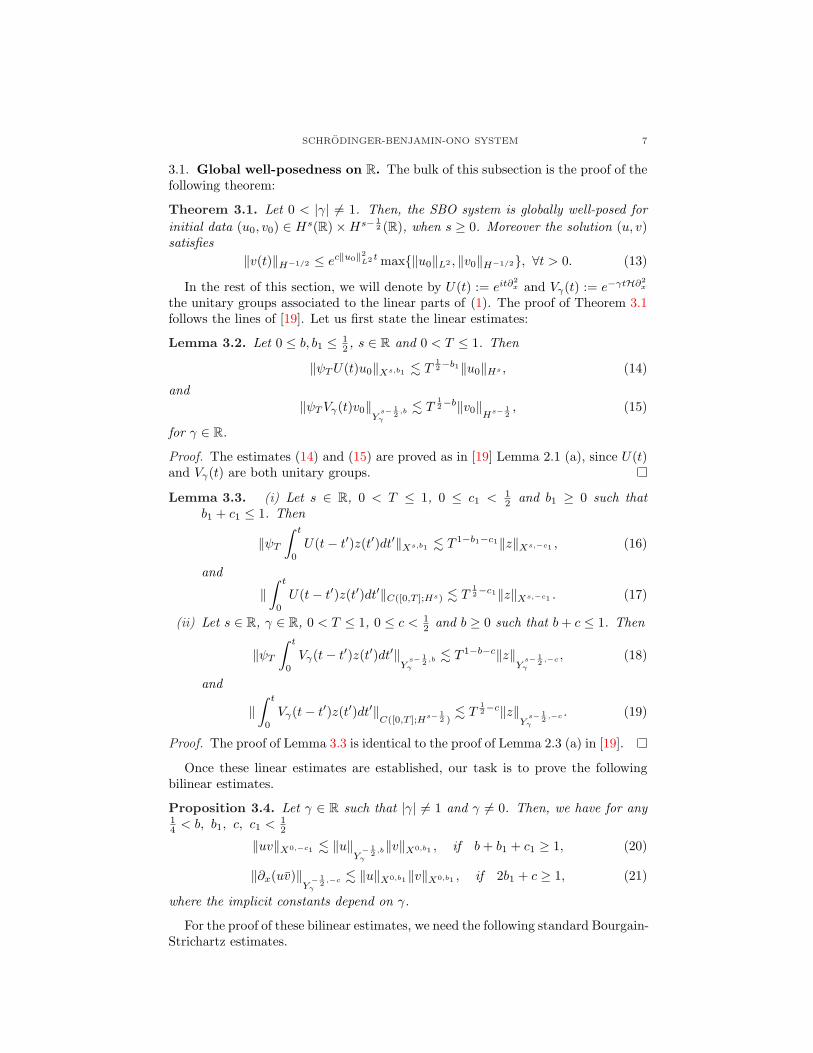
3.1. Global well-posedness on R. The bulk of this subsection is the proof of thefollowing theorem:
Theorem 3.1. Let 0 < |γ| 6= 1. Then, the SBO system is globally well-posed forinitial data (u0, v0) ∈ Hs(R)×Hs− 1
2 (R), when s ≥ 0. Moreover the solution (u, v)satisfies
‖v(t)‖H−1/2 ≤ ec‖u0‖2L2 t max‖u0‖L2 , ‖v0‖H−1/2, ∀t > 0. (13)
In the rest of this section, we will denote by U(t) := eit∂2x and Vγ(t) := e−γtH∂2
x
the unitary groups associated to the linear parts of (1). The proof of Theorem 3.1follows the lines of [19]. Let us first state the linear estimates:
Lemma 3.2. Let 0 ≤ b, b1 ≤ 12 , s ∈ R and 0 < T ≤ 1. Then
‖ψT U(t)u0‖Xs,b1 . T12−b1‖u0‖Hs , (14)
and‖ψT Vγ(t)v0‖
Ys− 1
2 ,bγ
. T12−b‖v0‖
Hs− 12, (15)
for γ ∈ R.
Proof. The estimates (14) and (15) are proved as in [19] Lemma 2.1 (a), since U(t)and Vγ(t) are both unitary groups.
Lemma 3.3. (i) Let s ∈ R, 0 < T ≤ 1, 0 ≤ c1 < 12 and b1 ≥ 0 such that
b1 + c1 ≤ 1. Then
‖ψT
∫ t
0
U(t− t′)z(t′)dt′‖Xs,b1 . T 1−b1−c1‖z‖Xs,−c1 , (16)
and
‖∫ t
0
U(t− t′)z(t′)dt′‖C([0,T ];Hs) . T12−c1‖z‖Xs,−c1 . (17)
(ii) Let s ∈ R, γ ∈ R, 0 < T ≤ 1, 0 ≤ c < 12 and b ≥ 0 such that b + c ≤ 1. Then
‖ψT
∫ t
0
Vγ(t− t′)z(t′)dt′‖Y
s− 12 ,b
γ
. T 1−b−c‖z‖Y
s− 12 ,−c
γ
, (18)
and
‖∫ t
0
Vγ(t− t′)z(t′)dt′‖C([0,T ];Hs− 1
2 ). T
12−c‖z‖
Ys− 1
2 ,−cγ
. (19)
Proof. The proof of Lemma 3.3 is identical to the proof of Lemma 2.3 (a) in [19].
Once these linear estimates are established, our task is to prove the followingbilinear estimates.
Proposition 3.4. Let γ ∈ R such that |γ| 6= 1 and γ 6= 0. Then, we have for any14 < b, b1, c, c1 < 1
2
‖uv‖X0,−c1 . ‖u‖Y− 1
2 ,bγ
‖v‖X0,b1 , if b + b1 + c1 ≥ 1, (20)
‖∂x(uv)‖Y− 1
2 ,−cγ
. ‖u‖X0,b1‖v‖X0,b1 , if 2b1 + c ≥ 1, (21)
where the implicit constants depend on γ.
For the proof of these bilinear estimates, we need the following standard Bourgain-Strichartz estimates.

8 J. ANGULO, C. MATHEUS AND D. PILOD
Proposition 3.5. Let γ ∈ R such that γ 6= 0. Then
‖u‖L3t,x
. ‖u‖X0,1/4+ , (22)
and‖u‖L3
t,x. ‖u‖
Y0,1/4+
γ. (23)
Proof. The estimate (22) is obtained by interpolating halfway between Strichartz’sestimate ‖u‖L6
x,t. ‖u‖X0,1/2+ and Plancherel’s identity ‖u‖L2
x,t= ‖u‖X0,0 . The
estimate (23) can be proved by a similar argument.
Finally, we recall the two following technical lemmas proved in [25].
Lemma 3.6. Let f ∈ Lq(R), g ∈ Lq′(R) with 1 ≤ q, q′ ≤ +∞ and 1q + 1
q′ = 1.Assume that f and g are nonnegative, even and nonincreasing for positive argument.Then f ∗ g enjoys the same property. In particular f ∗ g takes its maximum at zero.
Lemma 3.7. Let 0 ≤ a1, a2 < 12 such that a1 + a2 > 1
2 . Then∫
R〈y − α〉−2a1〈y − β〉−2a2 . 〈α− β〉1−2(a1+a2), ∀ α, β ∈ R.
Proof of Proposition 3.4. Without loss of generality we can suppose that |γ| < 1 inthe rest of the proof.
We first begin with the proof of the estimate (20). Letting f(τ, ξ) = 〈ξ〉−1/2〈τ +γξ|ξ|〉bu(τ, ξ), g(τ, ξ) = 〈τ + ξ2〉b1 v(τ, ξ) and using duality, we deduce that (20) isequivalent to
I . ‖f‖L2τ,ξ‖g‖L2
τ,ξ‖h‖L2
τ,ξ, (24)
where
I =∫
R4
h(τ, ξ)〈ξ1〉1/2f(τ1, ξ1)g(τ2, ξ2)〈σ〉c1〈σ1〉b〈σ2〉b1 dξdξ1dτdτ1, (25)
with ξ2 = ξ − ξ1, τ2 = τ − τ1, σ = τ + ξ2, σ1 = τ1 + γ|ξ1|ξ1 and σ2 = τ2 + ξ22 . The
algebraic relation associated to (25) is given by
− σ + σ1 + σ2 = −ξ2 + γ|ξ1|ξ1 + ξ22 . (26)
We split the integration domain R4 in the following regions
A = (τ, τ1, ξ, ξ1) ∈ R4 : |ξ1| ≤ 1,B = (τ, τ1, ξ, ξ1) ∈ R4 : |ξ1| > 1 and |σ1| = max(|σ|, |σ1|, |σ2|),C = (τ, τ1, ξ, ξ1) ∈ R4 : |ξ1| > 1 and |σ| = max(|σ|, |σ1|, |σ2|),D = (τ, τ1, ξ, ξ1) ∈ R4 : |ξ1| > 1 and |σ2| = max(|σ|, |σ1|, |σ2|),
and denote by IA, IB, IC and ID the restriction of I to each one of these regions.Estimate for IA. In this region 〈ξ1〉 ≤ 1, then we deduce using Plancherel’s identityand Holder’s inequality that
IA .∫
R2
(h(τ, ξ)
〈τ + ξ2〉c1
)∨(f(τ, ξ)
〈τ + γ|ξ|ξ〉b)∨(
g(τ, ξ)〈τ + ξ2〉b1
)∨dtdx
. ‖(
h(τ, ξ)〈τ + ξ2〉c1
)∨‖L3
t,x‖
(f(τ, ξ)
〈τ + γ|ξ|ξ〉b)∨
‖L3t,x‖
(g(τ, ξ)
〈τ + ξ2〉b1)∨
‖L3t,x
.
This implies, together with (22) and (23), that
IA . ‖f‖L2τ,ξ‖g‖L2
τ,ξ‖h‖L2
τ,ξ, (27)

SCHRODINGER-BENJAMIN-ONO SYSTEM 9
since b, b1, c1 > 14 .
Estimate for IB. Using the Cauchy-Schwarz inequality twice, we deduce that
IB .(
supξ1,σ1
〈σ1〉−2b
∫
R2
|ξ1|〈σ〉2c1〈σ2〉2b1
dξdσ
) 12
‖f‖L2τ,ξ‖g‖L2
τ,ξ‖h‖L2
τ,ξ. (28)
Recalling the algebraic relation (26), we have for ξ1, σ, σ1 fixed that dσ2 = −2ξ1dξ.Thus we obtain, by change of variables in the inner integral of the right-hand sideof (28),
〈σ1〉−2b
∫
R2
|ξ1|〈σ〉2c1〈σ2〉2b1
dξdσ
. 〈σ1〉−2b
(∫
|σ|≤|σ1|
dσ
〈σ〉2c1
)(∫
|σ2|≤|σ1|
dσ2
〈σ2〉2b1
). 〈σ1〉2(1−(b+b1+c1)) . 1,
since b + b1 + c1 ≥ 1. Combining this estimate with (28), we have
IB . ‖f‖L2τ,ξ‖g‖L2
τ,ξ‖h‖L2
τ,ξ. (29)
Estimate for IC. By the Cauchy-Schwarz inequality (applied two times) it is suffi-cient to bound
〈σ〉−2c1
∫
R2
|ξ1|〈σ1〉2b〈σ2〉2b1
dξ1dσ1 (30)
independently of ξ and σ to obtain that
IC . ‖f‖L2τ,ξ‖g‖L2
τ,ξ‖h‖L2
τ,ξ. (31)
Now following [10], we first treat the subregion |2((1 + γsgn(ξ1))ξ1 − ξ)| ≥1−|γ|
2 |ξ1|. When ξ, σ and σ1 are fixed, the identity (26) implies that
dσ2 = 2((1 + γsgn(ξ1))ξ1 − ξ)dξ1.
Hence we deduce that
〈σ〉−2c1
∫
R2
|ξ1|〈σ1〉2b〈σ2〉2b1
dξ1dσ1
. 〈σ〉−2c1
(∫
|σ1|≤|σ|
dσ1
〈σ1〉2b
)(∫
|σ2|≤|σ|
dσ2
〈σ2〉2b1
). 〈σ〉2(1−(b+b1+c1)),
which is bounded since b + b1 + c1 ≥ 1.In the subregion of C where |2((1 + γsgn(ξ1))ξ1 − ξ)| < 1−|γ|
2 |ξ1|, we have from(26) that
|ξ1|2 . |ξ21 + γ|ξ1|ξ1 − 2ξξ1| . |σ|.
Then, we obtain (by applying Lemma 3.7):
〈σ〉−2c1
∫
R2
|ξ1|〈σ1〉2b〈σ2〉2b1
dξ1dσ1 . 〈σ〉 12−2c1
∫
R
(∫
R〈σ1〉−2b〈σ2〉−2b1dσ1
)dξ1
. 〈σ〉 12−2c1
∫
R〈σ + ξ2
1 + γ|ξ1|ξ1 − 2ξξ1〉1−2(b+b1)dξ1.

10 J. ANGULO, C. MATHEUS AND D. PILOD
Performing the change of variable y = (θξ1 − θ−1ξ)2, where θ = (1 + sgn(ξ1)γ)12
and noticing that |y| . |σ| and dy = 2θ|y| 12 dξ1 we deduce that
〈σ〉−2c1
∫
R2
|ξ1|〈σ1〉2b〈σ2〉2b1
dξ1dσ1
. 〈σ〉 12−2c1
∫
|y|.|σ|
dy
|y| 12 〈y − θ−2ξ2 + σ〉−(1−2(b+b1)).
Now we use Lemma 3.6 to bound the right-hand side integral by∫
|y|.|σ||y|− 1
2 〈y〉1−(2(b+b1))dy . 〈σ〉[ 32−2(b+b1)]+ ,
where [α]+ = α if α > 0, [α]+ = ε arbitrarily small if α = 0, and [α]+ = 0 if α < 0.Therefore
〈σ〉−2c1
∫
R2
|ξ1|〈σ1〉2b〈σ2〉2b1
dξ1dσ1 . 〈σ〉 12−2c1+[ 32−2(b+b1)]+
which is always bounded using the assumptions on b, b1 and c1.Estimate for ID. By the Cauchy-Schwarz inequality it suffices to bound
〈σ2〉−2b1
∫
R2
|ξ1|〈σ1〉2b〈σ〉2c1
dξ1dσ1 (32)
independently of ξ2 and σ2.We first treat the subregion |2((1− γsgn(ξ1))ξ1 + ξ2)| ≥ 1−|γ|
2 |ξ1|. When ξ2, σ2
and σ are fixed, the identity (26) implies that
dσ = 2(ξ1 + ξ2 − γsgn(ξ1)ξ1)dξ1
Thus we can estimate (32) by
〈σ2〉−2b1
(∫
|σ1|≤|σ2|
dσ1
〈σ1〉2b
)(∫
|σ|≤|σ2|
dσ
〈σ〉2c1
). 〈σ〉2(1−(b+b1+c1)),
which is bounded since b + b1 + c1 ≥ 1.In the subregion |2((1−γsgn(ξ1))ξ1 +ξ2)| < 1−|γ|
2 |ξ1|, using (26), we deduce that
|ξ1|2 . |ξ21 − γ|ξ1|ξ1 + 2ξ2ξ1| . |σ2|,
where the implicit constant depends on γ. Then, Lemma 3.7 implies that
〈σ2〉−2b1
∫
R2
|ξ1|〈σ1〉2b〈σ〉2c1
dξ1dσ1 . 〈σ2〉 12−2b1
∫
R
(∫
R〈σ1〉−2b〈σ〉−2c1dσ1
)dξ1
. 〈σ2〉 12−2b1
∫
R〈σ2 + (1− γsgn(ξ1))ξ2
1 + 2ξ2ξ1〉1−2(b+c1)dξ1.
We perform the change of variable y = (θξ1 + θ−1ξ2)2 where θ = (1 − γsgn(ξ1))12
in the last integral and we use Lemma 3.6 plus the assumptions on b, b1 and c1 tobound (32) by
〈σ2〉 12−2b1
∫
|y|.|σ2||y|− 1
2 〈y − θ−2ξ22 + σ2〉1−2(b+c1) . 〈σ2〉 1
2−2b1+[ 32−2(b+c1)]+ . 1.
Therefore, we deduce that
ID . ‖f‖L2τ,ξ‖g‖L2
τ,ξ‖h‖L2
τ,ξ,
which, combined with (27), (29), and (31), implies (20).
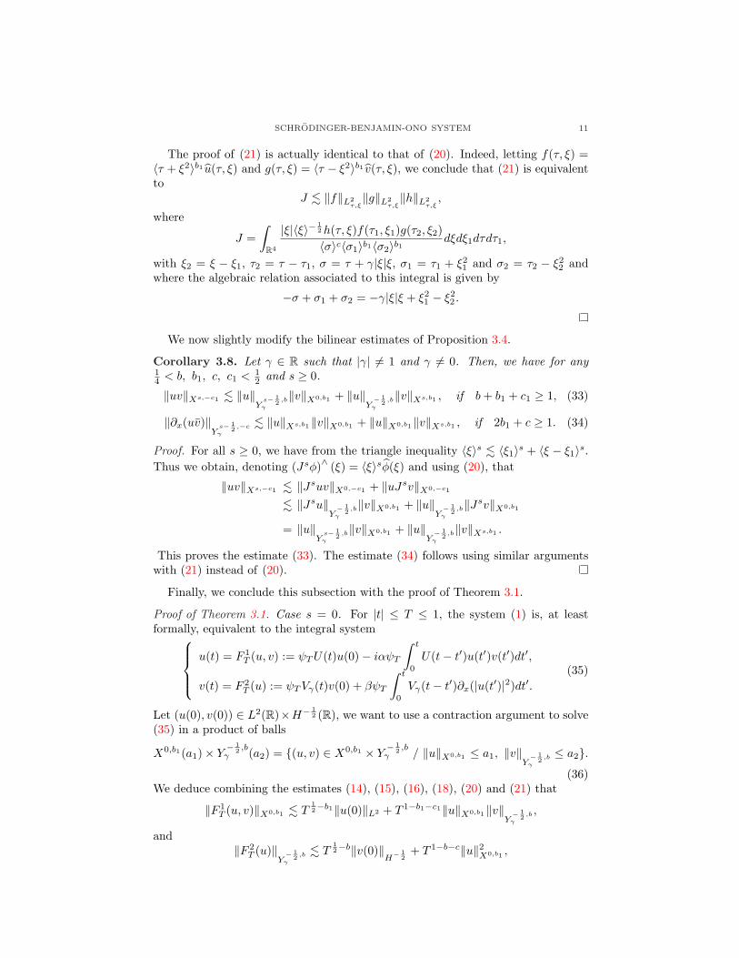
SCHRODINGER-BENJAMIN-ONO SYSTEM 11
The proof of (21) is actually identical to that of (20). Indeed, letting f(τ, ξ) =〈τ + ξ2〉b1 u(τ, ξ) and g(τ, ξ) = 〈τ − ξ2〉b1 v(τ, ξ), we conclude that (21) is equivalentto
J . ‖f‖L2τ,ξ‖g‖L2
τ,ξ‖h‖L2
τ,ξ,
where
J =∫
R4
|ξ|〈ξ〉− 12 h(τ, ξ)f(τ1, ξ1)g(τ2, ξ2)〈σ〉c〈σ1〉b1〈σ2〉b1 dξdξ1dτdτ1,
with ξ2 = ξ − ξ1, τ2 = τ − τ1, σ = τ + γ|ξ|ξ, σ1 = τ1 + ξ21 and σ2 = τ2 − ξ2
2 andwhere the algebraic relation associated to this integral is given by
−σ + σ1 + σ2 = −γ|ξ|ξ + ξ21 − ξ2
2 .
We now slightly modify the bilinear estimates of Proposition 3.4.
Corollary 3.8. Let γ ∈ R such that |γ| 6= 1 and γ 6= 0. Then, we have for any14 < b, b1, c, c1 < 1
2 and s ≥ 0.
‖uv‖Xs,−c1 . ‖u‖Y
s− 12 ,b
γ
‖v‖X0,b1 + ‖u‖Y− 1
2 ,bγ
‖v‖Xs,b1 , if b + b1 + c1 ≥ 1, (33)
‖∂x(uv)‖Y
s− 12 ,−c
γ
. ‖u‖Xs,b1‖v‖X0,b1 + ‖u‖X0,b1‖v‖Xs,b1 , if 2b1 + c ≥ 1. (34)
Proof. For all s ≥ 0, we have from the triangle inequality 〈ξ〉s . 〈ξ1〉s + 〈ξ − ξ1〉s.Thus we obtain, denoting (Jsφ)∧ (ξ) = 〈ξ〉sφ(ξ) and using (20), that
‖uv‖Xs,−c1 . ‖Jsuv‖X0,−c1 + ‖uJsv‖X0,−c1
. ‖Jsu‖Y− 1
2 ,bγ
‖v‖X0,b1 + ‖u‖Y− 1
2 ,bγ
‖Jsv‖X0,b1
= ‖u‖Y
s− 12 ,b
γ
‖v‖X0,b1 + ‖u‖Y− 1
2 ,bγ
‖v‖Xs,b1 .
This proves the estimate (33). The estimate (34) follows using similar argumentswith (21) instead of (20).
Finally, we conclude this subsection with the proof of Theorem 3.1.
Proof of Theorem 3.1. Case s = 0. For |t| ≤ T ≤ 1, the system (1) is, at leastformally, equivalent to the integral system
u(t) = F 1T (u, v) := ψT U(t)u(0)− iαψT
∫ t
0
U(t− t′)u(t′)v(t′)dt′,
v(t) = F 2T (u) := ψT Vγ(t)v(0) + βψT
∫ t
0
Vγ(t− t′)∂x(|u(t′)|2)dt′.(35)
Let (u(0), v(0)) ∈ L2(R)×H− 12 (R), we want to use a contraction argument to solve
(35) in a product of balls
X0,b1(a1)× Y− 1
2 ,bγ (a2) = (u, v) ∈ X0,b1 × Y
− 12 ,b
γ / ‖u‖X0,b1 ≤ a1, ‖v‖Y− 1
2 ,bγ
≤ a2.(36)
We deduce combining the estimates (14), (15), (16), (18), (20) and (21) that
‖F 1T (u, v)‖X0,b1 . T
12−b1‖u(0)‖L2 + T 1−b1−c1‖u‖X0,b1‖v‖
Y− 1
2 ,bγ
,
and‖F 2
T (u)‖Y− 1
2 ,bγ
. T12−b‖v(0)‖
H− 12
+ T 1−b−c‖u‖2X0,b1 ,
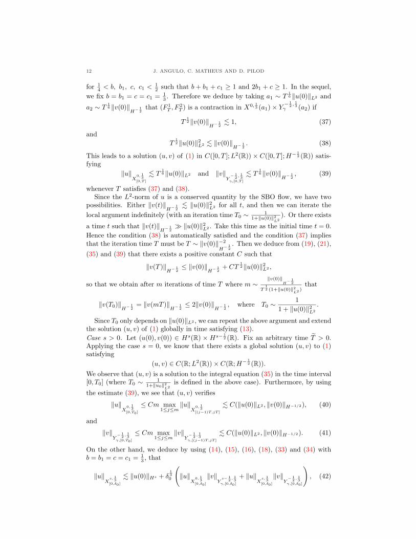
12 J. ANGULO, C. MATHEUS AND D. PILOD
for 14 < b, b1, c, c1 < 1
2 such that b + b1 + c1 ≥ 1 and 2b1 + c ≥ 1. In the sequel,we fix b = b1 = c = c1 = 1
3 . Therefore we deduce by taking a1 ∼ T16 ‖u(0)‖L2 and
a2 ∼ T16 ‖v(0)‖
H− 12
that (F 1T , F 2
T ) is a contraction in X0, 13 (a1)× Y
− 12 , 1
3γ (a2) if
T12 ‖v(0)‖
H− 12
. 1, (37)
andT
12 ‖u(0)‖2L2 . ‖v(0)‖
H− 12. (38)
This leads to a solution (u, v) of (1) in C([0, T ];L2(R)) × C([0, T ];H− 12 (R)) satis-
fying‖u‖
X0, 1
3[0,T ]
. T16 ‖u(0)‖L2 and ‖v‖
Y− 1
2 , 13
γ,[0,T ]
. T16 ‖v(0)‖
H− 12, (39)
whenever T satisfies (37) and (38).Since the L2-norm of u is a conserved quantity by the SBO flow, we have two
possibilities. Either ‖v(t)‖H− 1
2. ‖u(0)‖2L2 for all t, and then we can iterate the
local argument indefinitely (with an iteration time T0 ∼ 11+‖u(0)‖2
L2). Or there exists
a time t such that ‖v(t)‖H− 1
2À ‖u(0)‖2L2 . Take this time as the initial time t = 0.
Hence the condition (38) is automatically satisfied and the condition (37) impliesthat the iteration time T must be T ∼ ‖v(0)‖−2
H− 12. Then we deduce from (19), (21),
(35) and (39) that there exists a positive constant C such that
‖v(T )‖H− 1
2≤ ‖v(0)‖
H− 12
+ CT12 ‖u(0)‖2L2 ,
so that we obtain after m iterations of time T where m ∼‖v(0)‖
H− 1
2
T12 (1+‖u(0)‖2
L2 )that
‖v(T0)‖H− 1
2= ‖v(mT )‖
H− 12≤ 2‖v(0)‖
H− 12, where T0 ∼ 1
1 + ‖u(0)‖2L2
.
Since T0 only depends on ‖u(0)‖L2 , we can repeat the above argument and extendthe solution (u, v) of (1) globally in time satisfying (13).Case s > 0. Let (u(0), v(0)) ∈ Hs(R) × Hs− 1
2 (R). Fix an arbitrary time T > 0.Applying the case s = 0, we know that there exists a global solution (u, v) to (1)satisfying
(u, v) ∈ C(R;L2(R))× C(R;H− 12 (R)).
We observe that (u, v) is a solution to the integral equation (35) in the time interval[0, T0] (where T0 ∼ 1
1+‖u0‖2L2
is defined in the above case). Furthermore, by using
the estimate (39), we see that (u, v) verifies
‖u‖X
0, 13
[0,T0]
≤ Cm max1≤j≤m
‖u‖X
0, 13
[(j−1)T,jT ]
. C(‖u(0)‖L2 , ‖v(0)‖H−1/2), (40)
and
‖v‖Y− 1
2 , 13
γ,[0,T0]
≤ Cm max1≤j≤m
‖v‖Y− 1
2 , 13
γ,[(j−1)T,jT ]
. C(‖u(0)‖L2 , ‖v(0)‖H−1/2). (41)
On the other hand, we deduce by using (14), (15), (16), (18), (33) and (34) withb = b1 = c = c1 = 1
3 , that
‖u‖X
s, 13
[0,δ0]
. ‖u(0)‖Hs + δ130
(‖u‖
X0, 1
3[0,δ0]
‖v‖Y
s− 12 , 1
3γ,[0,δ0]
+ ‖u‖X
s, 13
[0,δ0]
‖v‖Y− 1
2 , 13
γ,[0,δ0]
), (42)

SCHRODINGER-BENJAMIN-ONO SYSTEM 13
and‖v‖
Ys− 1
2 , 13
γ,[0,δ0]
. ‖v(0)‖Hs− 1
2+ δ
130 ‖u‖
X0, 1
3[0,δ0]
‖u‖X
s, 13
[0,δ0]
, (43)
where 0 < δ0 ≤ T0. Inserting the estimate (43) into (42) and recalling (40), (41),we get that
‖u‖X
s, 13
[0,δ0]
. ‖u(0)‖Hs + C(‖u(0)‖L2 , ‖v(0)‖H−1/2)‖v(0)‖Hs− 1
2
+δ130 C(‖u(0)‖L2 , ‖v(0)‖
H− 12, T )‖u‖
Xs, 1
3[0,δ0]
.
Thus, if we choose
δ0 ∼ 11 + C(‖u(0)‖L2 , ‖v(0)‖
H− 12, T )3
, (44)
we deduce the a priori estimates
‖u‖X
s, 13
[0,δ0]
. ‖u(0)‖Hs + C(‖u(0)‖L2 , ‖v(0)‖H−1/2)‖v(0)‖Hs− 1
2,
and
‖v‖Y
s− 12 , 1
3γ,[0,δ0]
. ‖v(0)‖Hs− 1
2+ C(‖u(0)‖L2 , ‖v(0)‖H−1/2)(‖u(0)‖Hs + ‖v(0)‖
Hs− 12).
Therefore we conclude from Lemma 3.3 that
(u, v) ∈ C([0, δ0];Hs(R))× C([0, δ0];Hs− 12 (R)).
Since δ0 defined in (44) only depends on ‖u(0)‖L2 , ‖v(0)‖H− 1
2and T , we can iterate
the above argument a finite number of times to deduce that
(u, v) ∈ C([0, T ];Hs(R))× C([0, T ];Hs− 12 (R)).
This completes the proof of Theorem 3.1 if one remembers that T > 0 is arbitrary.
3.2. Well-posedness on T. This subsection contains sharp bilinear estimates forthe coupling terms uv and ∂x(|u|2) of the SBO system in the periodic setting andthe global well-posedness result in the energy space H1(T) × H1/2(T) (which isnecessary for our subsequent stability theory).
Theorem 3.9 (Local well-posedness in T). Let γ ∈ R such that γ 6= 0, |γ| 6= 1 ands ≥ 1/2. Then, the SBO system (1) is locally well-posed in Hs(T)×Hs−1/2(T), i.e.for all (u(0), v(0)) ∈ Hs(T)×Hs−1/2(T), there exists T = T (‖u(0)‖Hs , ‖v(0)‖Hs−1/2)and a unique solution of the Cauchy problem (1) of the form (ψT u, ψT v) such that(u, v) ∈ X
s,1/2+per × Y
s−1/2,1/2+γ,per . Moreover, (u, v) satisfies the additional regularity
(u, v) ∈ C([0, T ];Hs(T))× C([0, T ];Hs−1/2(T)) (45)
and the map solution S : (u(0), v(0)) 7→ (u, v) is smooth.
Using the conservation laws (2) as in [35], our local existence result implies
Theorem 3.10 (Global well-posedness in T). Let α, β, γ ∈ R such that γ 6= 0,|γ| 6= 1 and αγ
β < 0. Then, the SBO system (1) is globally well-posed in Hs(T) ×Hs−1/2(T), when s ≥ 1.
The fundamental technical points in the proof of Theorem 3.9 are the followingbilinear estimates. The rest of the proof follows by standard arguments, as in [20].

14 J. ANGULO, C. MATHEUS AND D. PILOD
Proposition 3.11. Let γ ∈ R such that γ 6= 0, |γ| 6= 1 and s ≥ 1/2. Then
‖uv‖X
s,−1/2+per
. ‖u‖Y
s−1/2,1/2γ,per
‖v‖X
s,1/2per
, (46)
‖∂x(uv)‖Y
s−1/2,−1/2+γ,per
. ‖u‖X
s,1/2per
‖v‖X
s,1/2per
, (47)
where the implicit constants depend on γ.
These estimates are sharp in the following sense
Proposition 3.12. Let γ 6= 0, |γ| 6= 1. Then(i) The estimate (46) fails for any s < 1/2.(ii) The estimate (47) fails for any s < 1/2.
Proposition 3.13. Let γ ∈ R such that |γ| = 1. Then(i) The estimate (46) fails for any s ∈ R.(ii) The estimate (47) fails for any s ∈ R.
The following Bourgain-Strichartz estimates will be used in the proof of Propo-sition 3.11.
Proposition 3.14. We have
‖u‖L4t,x
. ‖u‖X0,3/8 , (48)
and‖u‖L4
t,x. ‖u‖
Y0,3/8
γ, (49)
for u : R× T→ C and γ ∈ R, γ 6= 0.
Proof. The first estimate of (48) was proved by Bourgain in [16] and the second oneis a simple consequence of the first one (see for example [33]).
Proof of Proposition 3.11. Fix s ≥ 1/2. Without loss of generality we can supposethat 0 < |γ| < 1 in the rest of the proof.
In order to prove (46), it is sufficient to prove that
‖uv‖X
s,−3/8per
= ‖ 〈n〉s〈τ + n2〉3/8
(uv)∧(τ, n)‖l2nL2τ
. ‖u‖Y
s−1/2,1/2γ,per
‖v‖X
s,1/2per
. (50)
Letting f(τ, n) = 〈n〉s−1/2〈τ + γn|n|〉1/2u(τ, n), g(τ, n) = 〈n〉s〈τ + n2〉1/2v(τ, n)and using duality, we deduce that the estimate (50) is equivalent to
I . ‖f‖L2τ l2n‖g‖L2
τ l2n‖h‖L2
τ l2n, (51)
where
I :=∑
n,n1∈Z
∫
R2
〈n〉sh(τ, n)f(τ1, n1)〈τ + n2〉3/8〈n1〉s−1/2〈τ1 + γ|n1|n1〉1/2
× g(τ2, n2)〈n2〉s〈τ2 + n2
2〉1/2dτdτ1, (52)
where τ2 = τ − τ1 and n2 = n−n1. In order to bound the integral in (52), we splitthe integration domain R2 × Z2 in the following regions,
M = (τ, τ1, n, n1) ∈ R2 × Z2 : n1 = 0 or |n| ≤ c(γ)−1|n2|,N = (τ, τ1, n, n1) ∈ R2 × Z2 : n1 6= 0 and |n2| ≤ c(γ)|n|,
where c(γ) is a positive constant depending on γ to be fixed later. We also denoteby IM and IN the integral I restricted to the regions M and N , respectively.

SCHRODINGER-BENJAMIN-ONO SYSTEM 15
Estimate on the region M. We observe that, since s ≥ 1/2, it holds 〈n〉s〈n1〉s−1/2〈n2〉s .
1 (where the implicit constant depends on γ) in the region M. Thus, we deducethat, using the Plancherel identity and the L2
t,xL4t,xL4
t,x-Holder inequality,
IM .∑
n,n1∈Z
∫
R2
h(τ, n)f(τ1, n1)g(τ2, n2)dτdτ1
〈τ + n2〉3/8〈τ1 + γ|n1|n1〉1/2〈τ2 + n22〉1/2
.∫
R×T
(h(τ, n)
〈τ + n2〉3/8
)∨(f(τ, n)
〈τ + γ|n|n〉1/2
)∨(g(τ, n)
〈τ + n2〉1/2
)∨dtdx
. ‖(
h(τ, n)〈τ + n2〉3/8
)∨‖L2
t,x‖
(f(τ, n)
〈τ + γ|n|n〉1/2
)∨‖L4
t,x‖
(g(τ, n)
〈τ + n2〉1/2
)∨‖L4
t,x.
This implies, together with Estimates (48) and (49), that
IM . ‖f‖L2τ l2n‖g‖L2
τ l2n‖h‖L2
τ l2n. (53)
Estimate on the region N . The dispersive smoothing effect associated to the SBOsystem (1) can be translated by the following algebraic relation
− (τ + n2) + (τ1 + γn1|n1|) + (τ2 + n22) = Qγ(n, n1), (54)
whereQγ(n, n1) = n2
2 + γ|n1|n1 − n2. (55)
We have in the region N , |n1| ≤ (1 + c(γ))|n|, so that
|Qγ(n, n1)| ≥(1− |γ|(1 + c(γ))2 − c(γ)2
)(1 + c(γ))−2|n1|2.
Now, we choose c(γ) positive, small enough such that
(1− |γ|(1 + c(γ))2 − c(γ)2
)=
1− |γ|2
,
which is possible since |γ| < 1. Therefore, we divide the region N in three partsaccordingly to which term of the left-hand side of (54) is dominant:
N1 = (τ, τ1, n, n1) ∈ N : |τ + n2| ≥ |τ1 + γ|n1|n1|, |τ2 + n22|,
N2 = (τ, τ1, n, n1) ∈ N : |τ1 + γ|n1|n1| ≥ |τ + n2|, |τ2 + n22|,
N3 = (τ, τ1, n, n1) ∈ N : |τ2 + n22| ≥ |τ + n2|, |τ1 + γ|n1|n1|.
We denote by IN1 , IN2 and IN3 the restriction of the integral I to the regions N1,N2 and N3, respectively.
In the region N1, we have 〈n〉s〈n1〉s−1/2〈n2〉s ×
1〈τ+n2〉3/8 . 1, so that we can conclude
IN1 . ‖f‖L2τ l2n‖g‖L2
τ l2n‖h‖L2
τ l2n, (56)
exactly as for IM. We note that 〈n〉s〈n1〉s−1/2〈n2〉s ×
1〈τ1+|n1|n1〉1/2 . 1 in the region N2.
Then, using the L4t,xL2
t,xL4t,x-Holder inequality, that
IN2 . ‖(
h(τ, n)〈τ + n2〉3/8
)∨‖L4
t,x‖f‖L2
τ l2n‖
(g(τ, n)
〈τ + n2〉1/2
)∨‖L4
t,x.
Combining this with (48), we obtain that
IN2 . ‖f‖L2τ l2n‖g‖L2
τ l2n‖h‖L2
τ l2n. (57)
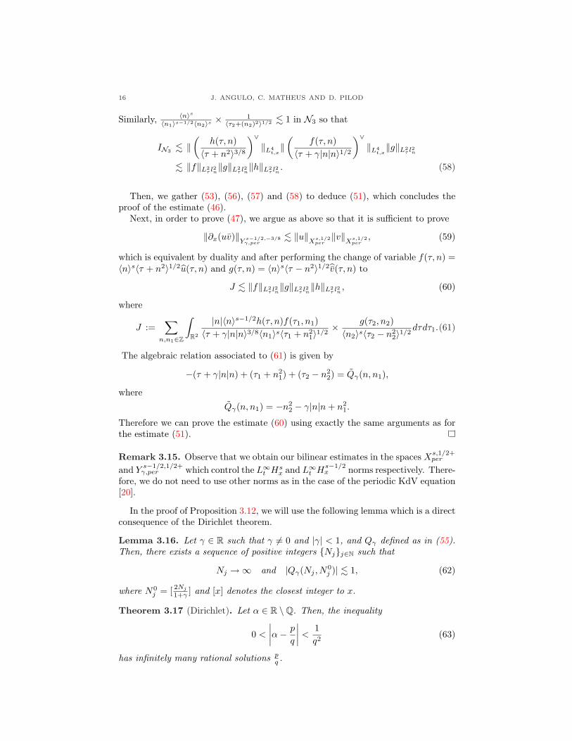
16 J. ANGULO, C. MATHEUS AND D. PILOD
Similarly, 〈n〉s〈n1〉s−1/2〈n2〉s ×
1〈τ2+(n2)2〉1/2 . 1 in N3 so that
IN3 . ‖(
h(τ, n)〈τ + n2〉3/8
)∨‖L4
t,x‖
(f(τ, n)
〈τ + γ|n|n〉1/2
)∨‖L4
t,x‖g‖L2
τ l2n
. ‖f‖L2τ l2n‖g‖L2
τ l2n‖h‖L2
τ l2n. (58)
Then, we gather (53), (56), (57) and (58) to deduce (51), which concludes theproof of the estimate (46).
Next, in order to prove (47), we argue as above so that it is sufficient to prove
‖∂x(uv)‖Y
s−1/2,−3/8γ,per
. ‖u‖X
s,1/2per
‖v‖X
s,1/2per
, (59)
which is equivalent by duality and after performing the change of variable f(τ, n) =〈n〉s〈τ + n2〉1/2u(τ, n) and g(τ, n) = 〈n〉s〈τ − n2〉1/2v(τ, n) to
J . ‖f‖L2τ l2n‖g‖L2
τ l2n‖h‖L2
τ l2n, (60)
where
J :=∑
n,n1∈Z
∫
R2
|n|〈n〉s−1/2h(τ, n)f(τ1, n1)〈τ + γ|n|n〉3/8〈n1〉s〈τ1 + n2
1〉1/2× g(τ2, n2)〈n2〉s〈τ2 − n2
2〉1/2dτdτ1.(61)
The algebraic relation associated to (61) is given by
−(τ + γ|n|n) + (τ1 + n21) + (τ2 − n2
2) = Qγ(n, n1),
whereQγ(n, n1) = −n2
2 − γ|n|n + n21.
Therefore we can prove the estimate (60) using exactly the same arguments as forthe estimate (51).
Remark 3.15. Observe that we obtain our bilinear estimates in the spaces Xs,1/2+per
and Ys−1/2,1/2+γ,per which control the L∞t Hs
x and L∞t Hs−1/2x norms respectively. There-
fore, we do not need to use other norms as in the case of the periodic KdV equation[20].
In the proof of Proposition 3.12, we will use the following lemma which is a directconsequence of the Dirichlet theorem.
Lemma 3.16. Let γ ∈ R such that γ 6= 0 and |γ| < 1, and Qγ defined as in (55).Then, there exists a sequence of positive integers Njj∈N such that
Nj →∞ and |Qγ(Nj , N0j )| . 1, (62)
where N0j = [ 2Nj
1+γ ] and [x] denotes the closest integer to x.
Theorem 3.17 (Dirichlet). Let α ∈ R \Q. Then, the inequality
0 <
∣∣∣∣α−p
q
∣∣∣∣ <1q2
(63)
has infinitely many rational solutions pq .

SCHRODINGER-BENJAMIN-ONO SYSTEM 17
Proof of Lemma 3.16. Fix γ ∈ R such that |γ| < 1. Let N a positive integer, N ≥ 2,α = 2
1+γ and N0 = [αN ]. Then, from the definition in (55), we deduce that
|Qγ(N, N0)| . 1 ⇐⇒∣∣∣∣α−
[αN ]N
∣∣∣∣ ≤1
N2. (64)
When α ∈ Q, α = pq , it is clear that we can find an infinity of positive integer N
satisfying the right-hand side of (64) choosing Nj = jq, j ∈ N. When α ∈ R \ Q,this is guaranteed by the Dirichlet theorem.
Proof of Proposition 3.12. We will only show that the estimate (46) fails, since acounterexample for the estimate (47) can be constructed in a similar way. Firstobserve that, letting f(τ, n) = 〈n〉s−1/2〈τ + γn|n|〉1/2u(τ, n) and g(τ, n) = 〈n〉s〈τ +n2〉1/2v(τ, n), the estimate (46) is equivalent to
‖Bγ(f, g; s)‖L2τ l2n
. ‖f‖L2τ l2n‖g‖L2
τ l2n, ∀ f, g ∈ L2
τ l2n, (65)
where
Bγ(f, g; s)(τ, n) :=〈n〉s
〈τ + n2〉1/2−∑
n1∈Z
∫
R
f(τ1, n1)〈n1〉s−1/2〈τ1 + γ|n1|n1〉1/2
× g(τ2, n2)〈n2〉s〈τ2 + n2
2〉1/2dτ1, (66)
and τ2 = τ − τ1, n2 = n− n1, for all s and γ ∈ R.Fix s < 1/2 and γ such that |γ| 6= 1; without loss of generality, we can suppose
that |γ| < 1. Consider the sequence of integer Nj obtained in Lemma 3.16. Notethat we can always assume Nj À 1. Define
fj(τ, n) = anχ1/2(τ + γ|n|n) with an =
1, n = N0j ,
0, elsewhere, (67)
and
gj(τ, n) = bnχ1/2(τ + n2) with bn =
1, n = Nj −N0j ,
0, elsewhere, (68)
where χr is the characteristic function of the interval [−r, r]. Hence,
‖fj‖L2τ l2n
∼ ‖gj‖L2τ l2n
∼ 1, (69)
an1bn−n1 6= 0 if and only if n1 = N0j and n = Nj .
Using (54), we deduce that∫
Rχ1/2(τ1 + γ|N0
j |N0j )χ1/2(τ − τ1 + (Nj −N0
j )2)dτ1 ∼ χ1(τ + N2 + Qγ(Nj , N0j )).
Therefore, we have from the definition in (66)
Bγ(fj , gj ; s)(τ, Nj) &Ns
j χ1(τ + N2j + Qγ(Nj , N
0j ))
〈τ + N2j 〉1/2−N
s−1/2j Ns
j
, (70)
where the implicit constant depends on γ. Thus, we deduce using (62) that
‖Bγ(fj , gj ; s)‖L2τ l2n
& N1/2−sj , ∀ j ∈ N (71)
which combined with (62) and (69) contradicts (65), since s < 1/2.
18 J. ANGULO, C. MATHEUS AND D. PILOD
Proof of Proposition 3.13. Let s ∈ R, we fix γ = 1. As in the proof of Proposition3.12, we will only show that the estimate (46) fails, since a counterexample for theestimate (47) can be constructed in a similar way. In this case, (46) is equivalent to
‖B1(f, g; s)‖L2τ l2n
. ‖f‖L2τ l2n‖g‖L2
τ l2n, ∀ f, g ∈ L2
τ l2n, (72)
where
B1(f, g; s)(τ, n) :=〈n〉s
〈τ + n2〉1/2−∑
n1∈Z
∫
R
f(τ1, n1)〈n1〉s−1/2〈τ1 + |n1|n1〉1/2
× g(τ2, n2)〈n2〉s〈τ2 + n2
2〉1/2dτ1, (73)
and τ2 = τ − τ1 and n2 = n− n1. Fix a positive integer N , such that N À 1, anddefine
fN (τ, n) = anχ1/2(τ + |n|n) with an =
1, n = N,0, elsewhere, (74)
and
gN (τ, n) = bnχ1/2(τ + n2) with bn =
1, n = 0,0, elsewhere, (75)
where χr is the characteristic function of the interval [−r, r]. Hence,
‖fN‖L2τ l2n
∼ ‖gN‖L2τ l2n
∼ 1, (76)
an1bn−n1 6= 0 if and only if n1 = N and n = N,
and ∫
Rχ1/2(τ1 + N2)χ1/2(τ − τ1)dτ1 ∼ χ1(τ + N2).
Therefore, we deduce from (73) that
‖B1(fN , gN ; s)‖L2τ l2n
& N1/2, ∀ N À 1, (77)
which combined with (76) contradicts (72). The case γ = −1 is similar.
Remark 3.18. Observe that the same counterexamples would prove that the es-timates (46) and (47) also fail whenever |γ| 6= 1, γ 6= 0 if s < 1/2 and whenever|γ| = 1 if s ∈ R, if we substitute −1/2+ by b′ and 1/2 by b for any b, b′ ∈ R (seealso [31] for similar results).
4. Existence of periodic traveling wave solutions. The goal of this section isto show the existence of a smooth branch of periodic traveling wave solutions for(5). Based on the ideas of Angulo in [4], we first show the existence of a smoothbranch of dnoidal waves solutions for (5) in the case γ = 0. Then by using theimplicit function theorem we construct (in the case γ 6= 0 and close to 0) a curveof periodic solutions for (5) bifurcating from these dnoidal waves.

SCHRODINGER-BENJAMIN-ONO SYSTEM 19
4.1. Dnoidal wave solutions. We start by finding solutions for the case γ = 0and σ > 0 in (5). Henceforth, without loss of generality, we will assume that α = 1and β = 1
2 . Hence, we will solve the system
φ′′0 − σφ0 = ψ0φ0
ψ0 = − 12cφ2
0.(78)
Then, by substituting the second equation of (78) into the first one, we obtain that
φ′′0 − σφ0 +12c
φ30 = 0. (79)
Equation (79) can be solved in a similar fashion to the method used by Angulo in[4] . For the sake of completeness, we provide here a sketch of the proof of this fact.Indeed, from (79), φ0 must satisfy the first-order equation
[φ′0]2 =
14c
[−φ40 + 4cσφ2
0 + 4cBφ0 ] =14c
(η21 − φ2
0)(φ20 − η2
2),
where Bφ0 is an integration constant and −η1, η1,−η2, η2 are the zeros of the poly-nomial F (t) = −t4 + 4cσt2 + 4cBφ0 . Moreover,
4cσ = η2
1 + η22
4cBφ0 = −η21η2
2 .(80)
Now, if we are looking for by φ0 to be a non-constant and smooth periodic solution,then η2 ≤ φ0 ≤ η1. So, by choosing η1 > η2 > 0 we obtain that φ0 is a positivesolution. Note that −φ0 is also a solution of (79). Next, define ζ = φ0/η1 andk2 = (η2
1 − η22)/η2
1 . It follows from (80) that
[ζ ′]2 = η21
4c (1− ζ2)(ζ2 + k2 − 1).
Now define χ through ζ2 = 1−k2 sin2 χ. So we get that 4c(χ′)2 = η21(1−k2 sin2 χ).
Then for l = η12√
c, and assuming that ζ(0) = 1, we have
∫ χ(ξ)
0
dt√1− k2sin2t
= l ξ.
Then from the definition of the Jacobian elliptic function sn(u; k), we have thatsinχ = sn(lξ; k) and hence ζ(ξ) =
√1− k2sn2(lξ; k) ≡ dn(lξ; k). Returning to the
variable φ0, we obtain the dnoidal wave solutions associated to equation (78),
φ0(ξ) ≡ φ0(ξ; η1, η2) = η1 dn( η1
2√
cξ; k
)
ψ0(ξ) ≡ ψ0(ξ; η1, η2) = −η21
2cdn2
( η1
2√
cξ; k
),
(81)
where
0 < η2 < η1, k2 =η21 − η2
2
η21
, η21 + η2
2 = 4cσ. (82)
Next, since dn has the fundamental period 2K(k), it follows that φ0 in (81) has thefundamental wavelength (i.e., period) Tφ0 given by
Tφ0 ≡4√
c
η1K(k).

20 J. ANGULO, C. MATHEUS AND D. PILOD
Given c > 0, σ > 0, it follows from (82) that 0 < η2 <√
2cσ < η1 < 2√
cσ.Moreover we can write
Tφ0(η2) =4√
c√4cσ − η2
2
K(k(η2)) with k2(η2) =4cσ − 2η2
2
4cσ − η22
. (83)
Then, using these formulas and the properties of the function K, we see that Tφ0 ∈(√
2σ π, +∞) for η2 ∈ (0,
√2cσ). Moreover, we will see in Theorem 4.1 below that
η2 7→ Tφ0(η2) is a strictly decreasing mapping and so we obtain the basic inequality
Tφ0 >
√2σ
π. (84)
Two relevant solutions of (78) are hidden in (81). Namely, the constant andsolitary wave solutions. Indeed, when η2 →
√2cσ, i.e. η2 → η1, it follows that
k → 0+. Then since d(u; 0+) → 1 we obtain the constant solutions
φ0(ξ) =√
2cσ and ψ0(ξ) = −σ. (85)
Next, for η2 → 0 we have η1 → 4cσ− and so k → 1−. Then since dn(u; 1−) →sech(u) we obtain the classical solitary wave solutions
φ0,s(ξ) = 2√
cσsech(√
σξ) and ψ0,s(ξ) = −2σsech2(√
σξ). (86)
Our next theorem is the main result of this subsection and it proves that for afixed period L > 0 there exists a smooth branch of dnoidal wave solutions with thesame minimal period L to (78). The construction is an immediate consequence of theimplicit function theorem. Indeed, fix c > 0 and ω ∈ R such that σ ≡ ω − c2/4 >
2π2/L2. Since the function η2 ∈ (0,√
2cσ) → Tφ0(η2) is strictly decreasing (seeproof of Theorem 4.1 below), there is a unique η2 = η2(σ) ∈ (0,
√2cσ) such that
φ0(·; η1(σ), η2(σ)) has the fundamental period Tφ0(η2(σ)) = L. Next, we claim thatthe choice of η2(σ) depends smoothly of σ:
Theorem 4.1. Let L and c be arbitrarily fixed positive numbers. Let σ0 > 2π2/L2
and η2,0 = η2(σ0) be the unique number in the interval (0,√
2cσ) such that Tφ0(η2,0) =L. Then,
(1) there are intervals I(σ0) and B(η2,0) around of σ0 and η2(σ0) respectively,and an unique smooth function Λ : I(σ0) → B(η2,0), such that Λ(σ0) = η2,0 and
4√
c√4cσ − η2
2
K(k(σ)) = L, (87)
where σ ∈ I(σ0), η2 = Λ(σ), and
k2 ≡ k2(σ) =4cσ − 2η2
2
4cσ − η22
∈ (0, 1). (88)
(2) Solutions (φ0(·; η1, η2), ψ0(·; η1, η2)) given by (81) and determined by η1 =η1(σ), η2 = η2(σ) = Λ(σ), with η2
1 + η22 = 4cσ, have the fundamental period L and
satisfy (78). Moreover, the mapping
σ ∈ I(σ0) → φ0(·; η1(σ), η2(σ)) ∈ Hnper([0, L])
is a smooth function (for all n ≥ 1 integer).(3) I(σ0) can be chosen as ( 2π2
L2 ,+∞).(4) The mapping Λ : I(σ0) → B(η2,0) is a strictly decreasing function. There-
fore, from (88), σ → k(σ) is a strictly increasing function.

SCHRODINGER-BENJAMIN-ONO SYSTEM 21
Proof. The key of the proof is to apply the implicit function theorem (Angulo [4]).Indeed, consider the open set Ω = (η, σ) : σ > 2π2
L2 , η ∈ (0,√
2cσ) ⊆ R2 anddefine Ψ : Ω → R by
Ψ(η, σ) =4√
c√4cσ − η2
K(k(η, σ)) (89)
where k2(η, σ) = 4cσ−2η2
4cσ−η2 . By hypotheses Ψ(η2,0, σ0) = L. Next, we show ∂ηΨ(η, σ) <
0. In fact, it is immediate that
∂ηΨ(η, σ) =4√
c η
(4cσ − η2)3/2K(k) +
4√
c√4cσ − η2
dK
dk
dk
dη.
Next, fromdk
dη= − 4cση
k(4cσ − η2)2,
and the relations (see [18])
dEdk = E−K
k , d2Edk2 = − 1
kdKdk ,
kk′2 d2Edk2 + k′2 dE
dk + kE = 0,(90)
with k′2 = 1− k2, and E = E(k) being the complete elliptic integral of second kinddefined as
E(k) =∫ 1
0
√1− k2t2
1− t2dt,
we have the following formal equivalences
∂ηΨ(η, σ) < 0 ⇔ k(4cσ − η2)(E − k
dE
dk
)< −4cσk
d2E
dk2
⇔ k(4cσ − η2)(E − k
dE
dk
)<
(dE
dk+
k
k′2E
)(4cσ − η2)(2− k2)
⇔ 2k′2dE
dk+ kE > 0 ⇔ dE
dk− k
d2E
dk2> 0 ⇔ dE
dk+
dK
dk> 0.
So, since the condition dEdk + dK
dk > 0 is equivalent to 2(1− k2)K(k) < (2− k2)E(k),which is easy to be obtained of the definitions of K and E.
Therefore, there is a unique smooth function, Λ, defined in a neighborhood I(σ0)of σ0, such that Ψ(Λ(σ), σ) = L for every σ ∈ I(σ0). So, we obtain (87). Moreover,since σ0 was chosen arbitrarily in I = ( 2π2
L2 ,+∞), it follows from the uniqueness ofthe function Λ that it can be extended to I.
Next, we show that Λ is a strictly decreasing function. We know that Ψ(Λ(σ), σ) =L for every σ ∈ I(σ0), then
d
dσΛ(σ) = −∂Ψ/∂σ
∂Ψ/∂η< 0 ⇔ ∂Ψ/∂σ < 0.
Thus, using the relation η2 = (4cσ − η2)(1 − k2) ≡ (4cσ − η2)k′2, we obtain thefollowing formal equivalences
∂Ψ∂σ
< 0 ⇔ (4cσ − η2)K >η2
k
dK
dk⇔ K >
k′2
k
dK
dk.
Then, since dKdk = (E − k′2K)/(kk′2), it follows that
∂Ψ∂σ
< 0 ⇔ k2K > E − k′2K ⇔ (k2 + k′2)K > E ⇔ K > E.

22 J. ANGULO, C. MATHEUS AND D. PILOD
This completes the proof of Theorem 4.1.
The following result will be used in our stability theory.
Corollary 4.2. Let L and c be arbitrarily fixed positive numbers. Consider thesmooth curve of dnoidal waves σ ∈ ( 2π2
L2 ,∞) → φ0(·; η1(σ), η2(σ)) determined byTheorem 4.1. Then
d
dσ
∫ L
0
φ20(ξ) dξ > 0.
Proof. By (81), (87), and the formula∫ K(k)
0dn2(x; k) dx = E(k) (see page 194 in
[18]) it follows that∫ L
0
φ20(ξ)dξ = 2η1
√c
∫ 2K(k)
0
dn2(x; k)dx =16cK
L
∫ K(k)
0
dn2(x; k)dx =16c
LE(k)K(k).
So, since k → K(k)E(k) and σ → k(σ) are strictly increasing functions we havethat
d
dσ
∫ L
0
φ20(ξ) dξ =
16c
L
d
dk[K(k)E(k)]
dk
dσ> 0.
4.2. Periodic traveling wave solutions for the equation (5). In this subsec-tion we show the existence of a branch of periodic traveling waves solutions of (5)for γ close to zero such that these solutions bifurcate the dnoidal waves solutionsfound in Theorem 78.
We start our analysis by studying the periodic eigenvalue problem considered on[0, L],
L0χ ≡ (− d2
dx2+ σ − 3
2cφ2
0)χ = λχ
χ(0) = χ(L), χ′(0) = χ′(L),(91)
where for σ > 2π2/L2, φ0 is given by Theorem 78 and satisfies (79).
Theorem 4.3. The linear operator L0 defined in (91) with domain H2per([0, L])
⊆ L2per([0, L]), has its first three eigenvalues simple with zero being its second ei-
genvalue (with eigenfunction ddxφ0). Moreover, the remainder of the spectrum is
constituted by a discrete set of eigenvalues which are double and converging to in-finity.
Proof. Theorem 4.3 is a consequence of the Floquet theory (see Angulo [4] andMagnus and Winkler [32]). Indeed, from the classical theory of compact symmetriclinear operator, we have that (91) determines a countable infinity set of eigenvaluesλn|n = 0, 1, 2, ... with λ0 ≤ λ1 ≤ λ2 ≤ λ3 ≤ λ4 ≤ ..., where double eigenvalue iscounted twice and λn → ∞ as n → ∞. We shall denote by χn the eigenfunctionassociated to the eigenvalue λn. From Sturm’s Oscillation Theory we have thatλ0 < λ1 ≤ λ2. Since L0
ddxφ0 = 0 and d
dxφ0 has 2 zeros in [0, L), it follows that 0is either λ1 or λ2 (see Theorem 3.1 in [4]). We will show that 0 = λ1 < λ2. So,we consider Ψ(x) ≡ χ(γx) with γ2 = 4c/η2
1 . Then from (91) and from the identityk2sn2x + dn2x = 1, we obtain
d2
dx2Ψ + [ρ− 6k2sn2(x; k)]Ψ = 0
Ψ(0) = Ψ(2K(k)), Ψ′(0) = Ψ′(2K(k)),(92)

SCHRODINGER-BENJAMIN-ONO SYSTEM 23
where
ρ =4c(λ− σ)
η21
+ 6. (93)
Now, from [32], it follows that (−∞, ρ0), (µ′0, µ′1) and (ρ1, ρ2) are the instability
intervals associated to this Lame’s equation, where for i ≥ 0, µ′i are the eigenvaluesassociated to the semi-periodic problem. Therefore, ρ0, ρ1, ρ2 are simple eigenvaluesfor (92) and the other eigenvalues ρ3 ≤ ρ4 < ρ5 ≤ ρ6 < · · · satisfy ρ3 = ρ4, ρ5 =ρ6, · · ·, i.e., they are double eigenvalues.
It is easy to verify that the first three eigenvalues ρ0, ρ1, ρ2 and its correspondingeigenfunctions Ψ0,Ψ1,Ψ2 are given by the formulas (see Ince [28])
ρ0 = 2[1 + k2 −√1− k2 + k4], Ψ0(x) = 1− (1 + k2 −√1− k2 + k4 )sn2(x),ρ1 = 4 + k2, Ψ1(x) = snx cnx,
ρ2 = 2[1 + k2 +√
1− k2 + k4], Ψ2(x) = 1− (1 + k2 +√
1− k2 + k4 )sn2(x).(94)
Next, Ψ0 has no zeros in [0, 2K] and Ψ2 has exactly 2 zeros in [0, 2K), then ρ0 isthe first eigenvalue to (92). Since ρ0 < ρ1 for every k2 ∈ (0, 1), we obtain from (93)and (82) that
4cλ0 = η21(k2 − 2− 2
√1− k2 + k4) < 0 ⇔ ρ0 < ρ1.
Therefore λ0 is the first negative eigenvalue to L0 with eigenfunction χ0(x) =Ψ0(x/γ). Similarly, since ρ1 < ρ2 for every k2 ∈ (0, 1), we obtain from (93) that
4cλ2 = η21(k2 − 2 + 2
√1− k2 + k4) > 0 ⇔ ρ1 < ρ2.
Hence λ2 is the third eigenvalue to L0 with eigenfunction χ2(x) = Ψ2(x/γ). Finally,since χ1(x) = Ψ1(x/γ) = µ d
dxφ0(x) we finish the proof.
Next, we have our theorem of existence of solutions for (5). For s ≥ 0, letHs
per,e([0, L]) denote the closed subspace of all even functions in Hsper([0, L]).
Theorem 4.4. Let L,α, β, c > 0 and σ > 2π2/L2 be fixed numbers. Then thereexist γ1 > 0 and a smooth branch
γ ∈ (−γ1, γ1) → (φγ , ψγ) ∈ H2per,e([0, L])×H1
per,e([0, L])
of solutions for Eq. (5). In particular, for γ → 0, (φγ , ψγ) converges to (φ0, ψ0)uniformly for x ∈ [0, L], where (φ0, ψ0) is given by Theorem 4.1 and it is defined by(81). Moreover, the mapping
γ ∈ (−γ1, γ1) → (d
dσφγ ,
d
dσψγ)
is continuous.
Proof. Without loss of generality, we take α = 1 and β = 1/2. Let Xe = H2per,e([0, L])×
H3per,e([0, L]) and define the map
G : R× (0,+∞)×Xe → L2per,e([0, L])×H2
per,e([0, L])
by
G(γ, λ, φ, ψ) = (−φ′′ + λφ + φψ,−γDψ + cψ +12φ2).

24 J. ANGULO, C. MATHEUS AND D. PILOD
A calculation shows that the Frechet derivative G(φ,ψ) = ∂G(γ, λ, φ, ψ)/∂(φ, ψ)exists and it is defined as a map from R × (0,+∞) ×Xe to B(Xe;L2
per,e([0, L]) ×H2
per,e([0, L])) by
G(φ,ψ)(γ, λ, φ, ψ) =
−
d2
dx2+ λ + ψ φ
φ −γD + c
.
¿From Theorem 4.1 it follows that for Φ0 = (φ0, ψ0), G(0, σ, Φ0) = ~0t. Moreover,from Theorem 4.3 we have that G(φ,ψ)(0, σ,Φ0) has a kernel generated by Φ′0
t.Next, since Φ′0 /∈ Xe, the boundedness of G(φ,ψ)(0, σ,Φ0)−1 follows trivially fromthe surjectivity of G(φ,ψ)(0, σ, Φ0) and the Open Mapping Theorem. Hence, sinceG and G(φ,ψ) are smooth maps on their domains, the Implicit Function Theoremimplies that there are γ1 > 0, λ1 ∈ (0, σ), and a smooth curve
(γ, λ) ∈ (−γ1, γ1)× (σ − λ1, σ + λ1) → (φγ,λ, ψγ,λ) ∈ Xe
such that G(γ, λ, φγ,λ, ψγ,λ) = 0. Then, for λ = σ we obtain a smooth branchγ ∈ (−γ1, γ1) → (φγ,σ, ψγ,σ) ≡ (φγ , ψγ) of solutions of (5) such that γ ∈ (−γ1, γ1) →( d
dσ φγ , ddσ ψγ) is continuous.
5. Stability of the periodic traveling wave solutions. We begin this sectiondefining the type of stability of our interest. For any c ∈ R+ define the functionsΦ(x) = eicx/2φ(x) and Ψ(x) = ψ(x), where (φ, ψ) is a solution of (5). Then we saythat the orbit generated by (Φ,Ψ), namely,
Ω(Φ,Ψ) = (eiθΦ(·+ x0),Ψ(·+ x0)) : (θ, x0) ∈ [0, 2π)× R,is stable in H1
per([0, L])×H12per([0, L]) by the flow generated by Eq. (1), if for every
ε > 0 there exists δ(ε) > 0 such that for (u0, v0) satisfying ‖u0 − Φ‖1 < δ and‖v0 − Ψ‖ 1
2< δ, we have that the global solution (u, v) of (1) with (u(0), v(0)) =
(u0, v0) satisfies that (u, v) ∈ C(R;H1per([0, L]))× C(R;H
12per([0, L])) and
infx0∈R,θ∈[0,2π)
‖eiθu(·+ x0, t)− Φ‖1 + ‖v(·+ x0, t)−Ψ‖ 12 < ε, (95)
for all t ∈ R.The main result to be proved in this section is that the periodic traveling waves
solutions of (1) determined by Theorem 4.4 are stable for σ > 2π2/L2 and γ negativeclose to 0.
Theorem 5.1. Let L,α, β, c > 0 and σ > 2π2/L2 be fixed numbers. We consider thesmooth curve of periodic traveling waves solutions for (5), γ → (φγ , ψγ), determinedby Theorem 4.4. Then there exists γ0 > 0 such that for each γ ∈ (−γ0, 0), the orbitgenerated by (Φγ(x),Ψγ(x)) with
Φγ(x) = eicx/2φγ(x) and Ψγ(x) = ψγ(x),
is orbitally stable in H1per([0, L])×H
12per([0, L]).
The proof of Theorem 5.1 is based on the ideas developed by Angulo in [8] (seealso Benjamin [12] and Weinstein [38]) which give us an easy form of manipulatingwith the required spectral information and the positivity property of the quantityd
dσ
∫φ2
γ(x)dx, which are basic in our stability theory. We do not use the abstractstability theory of Grillakis et al. basically by these circumstances. So, we consider

SCHRODINGER-BENJAMIN-ONO SYSTEM 25
(φγ , ψγ) a solution of (5) obtained in Theorem 4.4. For (u0, v0) ∈ H1per([0, L]) ×
H12per([0, L]) and the global solution (u, v) to (1) corresponding to these initial data
given by Theorem 3.10, we define for t ≥ 0 and σ > 2π2/L2
Ωt(x0, θ) = ‖eiθ(Tcu)′(·+ x0, t)− φ′γ‖2 + σ‖eiθ(Tcu)(·+ x0, t)− φγ‖2 (96)
where we denote by Tc the bounded linear operator defined by
(Tcu)(x, t) = e−ic(x−ct)/2u(x, t).
Then, the deviation of the solution u(t) from the orbit generated by Φ is measuredby
ρσ(u(·, t), φγ)2 ≡ infx0∈[0,L],θ∈[0,2π]
Ωt(x0, θ). (97)
Hence, since Ωt is continuous on [0, L]× [0, 2π] we have that the infimum in (97) isattained in (x0, θ) = (x0(t), θ(t)).
Proof of Theorem 5.1. Consider the perturbation of the periodic traveling wave(φγ , ψγ)
ξ(x, t) = eiθ(Tcu)(x + x0, t)− φγ(x)η(x, t) = v(x + x0, t)− ψγ(x). (98)
Hence, by the property of minimum of (x0, θ) = (x0(t), θ(t)), we obtain from (98)that p(x, t) = Re(ξ(x, t)) and q(x, t) = Im(ξ(x, t)) satisfy the compatibility relations
∫ L
0
q(x, t)φγ(x)ψγ(x) dx = 0∫ L
0
p(x, t)(φγ(x)ψγ(x))′ dx = 0.
(99)
Now we take the continuous functional L defined on H1per([0, L]) × H
12per([0, L])
byL(u, v) = E(u, v) + c G(u, v) + ω H(u, v),
where E, G,H are defined by (2). Then, from (98) and (5), we have
∆L(t) := L(u(t), v(t))− L(Φγ ,Ψγ) = L(Φγ + eicx/2ξ, ψγ + η)− L(Φγ , ψγ)
= < Lγp, p > + < L+γ q, q >
+α
2β
∫ L
0
[K1/2
γ η + 2βK−1/2γ (φγp) + βK−1/2
γ (p2 + q2)]2
dx
−αβ
2
∫ L
0
[|K−1/2
γ (p2 + q2)|2 + 4K−1/2γ (φγp)K−1/2
γ (p2 + q2)]dx, (100)
where, for γ < 0 we define K−1γ as
K−1γ f(k) =
1−γ|k|+ c
f(k) for k ∈ Z,
which is the inverse operator of Kγ : Hsper([0, L]) → Hs−1
per ([0, L]) defined by Kγ =−γD + c. The operator Lγ is
Lγ = − d2
dx2+ σ + αψγ − 2αβφγ K−1
γ φγ , (101)

26 J. ANGULO, C. MATHEUS AND D. PILOD
with φγ K−1γ φγ given by [φγ K−1
γ φγ ](f) = φγK−1γ (φγf). Here L+
γ is definedby
L+γ = − d2
dx2+ σ + αψγ (102)
and K1/2γ , K−1/2
γ are the positive roots of Kγ and K−1γ respectively.
Now, we need to find a lower bound for ∆L(t). The first step will be to obtain asuitable lower bound of the last term on the right-hand side of (100). In fact, sinceK−1/2
γ is a bounded operator on L2per([0, L]), φγ is uniformly bounded, and from
the continuous embedding of H1per([0, L]) in L4
per([0, L]) in L∞([0, L]), we have that
−αβ
2
∫ L
0
[|K−1/2
γ (p2 + q2)|2 + 4K−1/2γ (φγp)K−1/2
γ (p2 + q2)]dx
≥ −C1‖ξ‖31 − C2‖ξ‖41 (103)
where C1 and C2 are positive constants.The estimates for 〈Lγp, p〉 and 〈L+
γ q, q〉 will be obtained from the following the-orem.
Lemma 5.2. Let L,α, β, c > 0 and σ > 2π2/L2 be fixed numbers. Then, there existsγ2 > 0 such that, if γ ∈ (−γ2, 0), the self-adjoint operators Lγ and L+
γ defined in(101) and (102), respectively, with domain H2
per([0, L]) have the following properties:(1) Lγ has a simple negative eigenvalue λγ with eigenfunction ϕγ and
∫ L
0φγϕγdx 6=
0.(2) Lγ has a simple eigenvalue at zero with eigenfunction d
dxφγ .(3) There is ηγ > 0 such that for βγ ∈ Σ(Lγ)− λγ , 0, we have that βγ > ηγ .(4) L+
γ is a non-negative operator which has zero as its first eigenvalue witheigenfunction φγ . The remainder of the spectrum is constituted by a discrete set ofeigenvalues.
Proof. The idea of the proof is to use the min-max principle. From (5) it followsthat Lγφγ = 2φγψγ and so since ψγ < 0 we have that for γ < 0, 〈Lγφγ , φγ〉 =2
∫R φ2
γψγdx < 0. Therefore Lγ has a negative eigenvalue. Moreover, Lγddxφγ = 0.
Next, for f ∈ H1per([0, L]) and ‖f‖ = 1, we have
〈Lγf, f〉 = 〈L0f, f〉 − γ
cα2〈φ0f,DK−1
γ (φ0f)〉+ α
∫ L
0
(ψγ − ψ0)f2dx
+α2
∫ L
0
[φ0fK−1γ (φ0f)− φγfK−1
γ (φγf)]dx
≥ 〈L0f, f〉+ α
∫ L
0
(ψγ − ψ0)f2dx + α2
∫ L
0
[φ0fK−1γ (φ0f)− φγfK−1
γ (φγf)]dx,
(104)where the last inequality is due to that γ < 0 and DK−1
γ is a positive operator. So,since
∣∣∣∫ L
0
(ψγ − ψ0)f2dx∣∣∣ ≤ ‖ψγ − ψ0‖∞
∣∣∣∫ L
0
[φ0fK−1γ (φ0f)− φγfK−1
γ (φγf)]dx∣∣∣ ≤ (‖φγ‖+ ‖φ0‖)‖φγ − φ0‖∞,
(105)
we have from Theorem 4.4 that for γ near 0− and ε small, 〈Lγf, f〉 ≥ 〈L0f, f〉 − ε.Hence, for f ⊥ χ0 and f ⊥ d
dxφ0, where L0χ0 = λ0χ0 with λ0 < 0, we have fromthe spectral structure of L0 (Theorem 4.3) that 〈Lγf, f〉 ≥ ηγ > 0. Therefore, from

SCHRODINGER-BENJAMIN-ONO SYSTEM 27
min-max principle ([36]) we obtain the desired spectral structure for Lγ . Moreover,let ϕγ be such that Lγϕγ = λγϕγ with λγ < 0. Therefore, if φγ ⊥ ϕγ then fromthe spectral structure of Lγ we must have that 〈Lγφγ , φγ〉 ≥ 0. But we know that〈Lγφγ , φγ〉 < 0. Hence, 〈φγ , ϕγ〉 6= 0. Finally, since L+
γ φγ = 0 with φγ > 0, itfollows that zero is simple and it is the first eigenvalue. It follows from the theoryof Hill’s equation (see [32]) that the remainder of the spectrum is discrete.
The next theorem follows the same ideas of Lemma 2.7 in [8].
Lemma 5.3. Consider γ < 0 close to zero such that Theorem 5.2 is true. Then
(a) inf 〈Lγf, f〉 : ‖f‖ = 1, 〈f, φγ〉 = 0, ≡ β0 = 0.
(b) inf 〈Lγf, f〉 : ‖f‖ = 1, 〈f, φγ〉 = 0, 〈f, (φγψγ)′〉 = 0 ≡ µ > 0.
Proof. Part (a). Since Lγddxφγ = 0 and 〈 d
dxφγ , φγ〉 = 0 then β0 ≤ 0. Next we showthat β0 ≥ 0 by using Lemma E.1 in Weinstein [39]. So, we shall show initially thatthe infimum is attained. Let ψj ⊆ H1
per([0, L]) with ‖ψj‖ = 1, 〈ψj , φγ〉 = 0 andlimj→∞〈Lγψj , ψj〉 = β0. Then there is a subsequence of ψj, which we denoteagain by ψj, such that ψj ψ weakly in H1
per([0, L]), so ψj → ψ in L2per([0, L]).
Hence ‖ψ‖ = 1 and 〈ψ, φγ〉 = 0. Since ‖ψ′‖2 ≤ lim inf ‖ψ′‖2 and K−1γ (φγψj) →
K−1γ (φγψ) in L2
per([0, L]), we have β0 ≤ 〈Lγψ, ψ〉 ≤ lim inf〈Lγψj , ψj〉 = β0. Next weshow that 〈L−1
γ φγ , φγ〉 ≤ 0. From (5) and Theorem 4.4 we obtain for χγ = − ddσ φγ
that Lγχγ = φγ . Moreover, from Corollary 4.2 it follows that 〈− ddσ φ0, φ0〉 < 0 and
so for γ small enough 〈− ddσ φγ , φγ〉 < 0. Hence from [39] we obtain that β0 ≥ 0.
This shows part (a) of the theorem.Part (b). From (a) we have that µ ≥ 0. Suppose µ = 0. Then following a similar
analysis to that used in part (a) above, we have that the infimum define in (b) isattained at an admissible function ζ. So, from Lagrange’s multiplier theory, thereare λ, θ, η such that
Lγζ = λζ + θφγ + η(φγψγ)′. (106)Using (106) and 〈Lγζ, ζ〉 = 0 we obtain that λ = 0. Taking the inner product of(106) with φ′γ , we have from Lγφ′γ = 0 that
0 = η
∫ L
0
φ′γ(φγψγ)′dx, (107)
but the integral in (107) converges to∫ L
0
φ′0(φ0ψ0)′dx =−3β
c
∫ L
0
φ20(φ
′0)
2dx < 0
as γ → 0 (see (5) and (78)). Then, from (107), we obtain η = 0 and therefore Lγζ =θφγ . So, since Lγ(− d
dσ φγ) = φγ , we obtain 0 = 〈ζ, φγ〉 = θ〈φγ ,− ddσ φγ〉. Therefore
θ = 0 and Lγζ = 0. Then ζ = νφ′γ for some ν 6= 0, which is a contradiction. Thusµ > 0 and the proof of the lemma is complete.
Theorem 5.4. Consider γ < 0 close to zero such that Lemma 5.2 is true. If L+γ
is defined as in (102) then
inf 〈L+γ f, f〉 : ‖f‖ = 1, 〈f, φγψγ〉 = 0 ≡ µ0 > 0.
Proof. The proof follows from Lemma 5.2 and the ideas in Lemma 2.8 in [8].

28 J. ANGULO, C. MATHEUS AND D. PILOD
Next we finish the proof of Theorem 5.1 by returning to (100). Our task is toestimate the terms 〈Lγp, p〉 and 〈L+
γ q, q〉 where p and q satisfy (99). From Theorem5.4 there is C1 > 0 such that
〈L+γ q, q〉 ≥ C1‖q‖21. (108)
Now we estimate 〈Lγp, p〉. Suppose without loss of generality that ‖φγ‖ = 1. Wewrite p⊥ = p − p|| , where p|| = 〈p, φγ〉φγ . Then, from (99), (5), and integrationby parts it follows that 〈p⊥ , (φγψγ)′〉 = 0. Therefore from Lemma 5.3, it follows〈Lγp⊥ , p⊥〉 ≥ β‖p⊥‖2. Now we suppose that ‖u0‖ = ‖φγ‖ = 1. Since ‖u(t)‖2 = 1for all t, we have that 〈p, φγ〉 = −‖ξ‖2/2. So, 〈Lγp⊥ , p⊥〉 ≥ β1‖p‖2−β2‖ξ‖41,σ. Since〈Lγφγ , φγ〉 < 0 it follows that 〈Lγp|| , p||〉 ≥ −β3‖ξ‖41,σ. Moreover, Cauchy-Schwarzinequality implies 〈Lγp|| , p⊥〉 ≥ −β4‖ξ‖31. Therefore we conclude from the specificform of Lγ that
〈Lγp, p〉 ≥ D1‖p‖21,σ −D2‖ξ‖31,σ −D3‖ξ‖41,σ, (109)
with Di > 0 and ‖f‖21,σ = ‖f ′‖2 + σ‖f‖2.Next, by collecting the results in (103), (108) and (109) and substituting them
in (100), we obtain
∆L(t) ≥ d1‖ξ‖21,σ − d2‖ξ‖31,σ − d3‖ξ‖41,σ, (110)
where di > 0. Therefore, from standard arguments ([15]), for any ε > 0, there existsδ(ε) > 0 such that, if ‖u0−Φγ‖1,σ < δ(ε) and ‖v0−Ψγ‖ 1
2< δ(ε), then for t ∈ [0,∞)
ρσ(u(t), φγ)2 = ‖ξ(t)‖21,σ < ε. (111)
Now, it follows from (100) and from the above analysis of ξ that
ε ≥ α
2β
∫ L
0
[K1/2
γ η + 2βK−1/2γ (φγp) + βK−1/2
γ (p2 + q2)]2
dx.
Thus, from (111) and the equivalence of the norms ‖K1/2γ η‖ and ‖η‖ 1
2, we ob-
tain (95). This proves that (Φγ ,Ψγ) is stable relative to small perturbation whichpreserves the L2
per([0, L]) norm of Φγ . The general case follows from that γ ∈(−γ1, γ1) → φγ is a continuous curve and d
dσ‖φγ‖2 > 0. ¤
Acknowledgements. The authors are grateful to the anonymous referee for hisvaluable comments and suggestions. Also, the authors would like to thank JamesColliander, Justin Holmer and Nikolaos Tzirakis for the interesting discussions con-cerning the Schrodinger-Benjamin-Ono system.
REFERENCES
[1] J. P. Albert, Positivity properties and stability of solitary-wave solutions of model equationsfor long waves, Comm. Part. Diff. Eq., 17 (1992), 1–22.
[2] J. P. Albert and J. L. Bona, Total positivity and the stability of internal waves in fluids of
finite depth, IMA J. Applied Math., 46 (1991), 1–19.[3] J. P. Albert, J. L. Bona and D. Henry, Sufficient conditions for stability of solitary-wave
equation of model equations for long waves, Physica D, 24 (1987), 343–366.[4] J. Angulo, Nonlinear stability of periodic traveling wave solutions to the Schrodinger and the
modified Korteweg-de Vries, J. Diff. Eq., 235 (2007), 1–30.
[5] J. Angulo, J. L. Bona and M. Scialom, Stability of cnoidal waves, Adv. Diff. Eq., 11 (2006),1321–1374.
[6] J. Angulo and F. Linares, Periodic pulses of coupled nonlinear Schrodinger equations in
optics, Indiana Univ. Math. J., 56 (2007), 847–877.

SCHRODINGER-BENJAMIN-ONO SYSTEM 29
[7] J. Angulo and F. Montenegro, Existence and evenness of solitary waves solutions for aninteraction equation of short and long dispersive waves, Nonlinearity, 13 (2000), 1595–1611.
[8] J. Angulo and F. Montenegro, Orbital stability of Solitary Wave Solutions for an Interactionequation of Short and Long Dispersive waves, J. Diff. Eq., 174 (2001), 181–199.
[9] D. Bekiranov, T. Ogawa and G. Ponce, On the well-posedness of Benney’s interaction equa-
tion of short and long waves, Adv. Diff. Eq., 1 (1996), 919–937.[10] D. Bekiranov, T. Ogawa and G. Ponce, Interaction equation for short and long dispersive
waves, J. Funct. Anal., 158 (1998), 357–388.
[11] T. B. Benjamin, Internal waves of permanent form in fluids of great depht, J. Fluid Mech.,29 (1967), 559–592.
[12] T. B. Benjamin, The stability of solitary waves, Proc. Roy. Soc. London A., 338 (1972),
153–183.[13] D. J. Benney, Significant interactions between small and large scale surface waves, Stud.
Appl. Math., 55 (1976), 93–106.
[14] D. J. Benney, A general theory for interactions between short and long waves, Stud. Appl.Math., 56 (1977), 81–94.
[15] J. L. Bona, On the stability theory of solitary waves, Proc. Roy. Soc. London Ser. A, 344(1975), 363–374.
[16] J. Bourgain, Fourier transform restriction phenomena for certain lattice subsets and appli-
cation to the nonlinear evolution equations I, II, Geom. Funct. Anal., 3 (1993), 107–156,209–262.
[17] J. Bourgain, “Global Solutions of Nonlinear Schrodinger Equations,” American Mathematical
Society Colloquium Publications, 46, Providence, RI, 1999.[18] P. F. Byrd and M. D. Friedman, “Handbook of Elliptic Integrals for Engineers and Scientists,”
2nd edition, Springer-Verlag, New York, 1971.[19] J. Colliander, J. Holmer and N. Tzirakis, Low regularity global well-posedness for the Za-
kharov and Klein-Gordon-Schrodinger systems, to appear in Transactions of AMS, preprint,arXiv::0603595.
[20] J. Colliander, M. Keel, G. Staffilani, H. Takaoka and T. Tao, Sharp global well-posedness for
KdV and modified KdV on R and T, J. Amer. Math. Soc., 16 (2003), 705–749.[21] V. D. Djordjevic and L. G. Redekopp, On two-dimensional packet of capillary-gravity waves,
J. Fluid Mech., 79 (1977), 703–714.
[22] M. Funakoshi and M. Oikawa, The resonant interaction between a long internal gravity wave
and a surface gravity wave packet, J. Phys. Soc. Japan, 52 (1983), 1982–1995.[23] T. Gallay and M. Haragus, Stability of small periodic waves for the nonlinear Schrodinger
equation, J. Diff. Eq., 234 (2007), 544–581.[24] T. Gallay and M. Haragus, Orbital Stability of periodic waves for the nonlinear Schrodinger
equation, J. Dyn. Diff. Eq., 19 (2007), 825–865.[25] J. Ginibre, Y. Tsutsumi and G. Velo, On the Cauchy problem for the Zakharov System, J.
Funct. Anal., 151 (1997), 384–436.[26] M. Grillakis, J. Shatah and W. Strauss, Stability theory of solitary waves in the presence of
symmetry II, J. Funct. Anal., 94 (1990), 308–348.[27] R. H. J. Grimshaw, The modulation of an internal gravity-wave packet and the resonance
with the mean motion, Stud. Appl. Math., 56 (1977), 241–266.
[28] E. L. Ince, The periodic Lame functions, Proc. Roy. Soc. Edinburgh, 60 (1940), 47–63.[29] R. J. Iorio and V. M. Iorio, “Fourier Analysis and Partial Differential Equations,” Cambridge
Stud. in Adv. Math., 70, 2001.
[30] V. I. Karpman, On the dynamics of sonic-Langmuir soliton, Phys. Scripta., 11 (1975), 263–265.
[31] C. E. Kenig, G. Ponce and L. Vega, A bilinear estimate with applications to the KdV equation,
J. Amer. Math. Soc., 9 (1996), 573–603.[32] W. Magnus, and S. Winkler, “Hill’s Equation,” Interscience, Tracts in Pure and Appl. Math.
Wiley, NY., 20, 1966.[33] L. Molinet, Global well-posedness in L2 for the periodic Benjamin-Ono equation, preprint,
arXiv::0601217.[34] H. Ono, Algebraic solitary waves in stratified fluids, J. Phys. Soc. Japan, 39 (1975), 1082–
1091.
[35] H. Pecher, Rough solutions of a Schrodinger-Benjamin-Ono system, Diff. Int. Eq., 19 (2006),
517–535.
30 J. ANGULO, C. MATHEUS AND D. PILOD
[36] Reed and B. Simon, “Methods of Modern Mathematical Physics: Analysis of Operator, v.IV”, Academic Press, 1978.
[37] T. Tao, Global well-posedness of the Benjamin-Ono equation in H1(R), J. Hyp. Diff. Eq., 1(2004), 27–49.
[38] M. I. Weinstein, Lyapunov stability of ground states of nonlinear dispersive evolution equa-
tions, Comm. Pure Appl. Math., 39 (1986), 51–68.[39] M. I. Weinstein, Modulational stability of ground states of nonlinear Schrodinger equations,
Siam J. Math. Anal., 16 (1985), 472–491.
[40] N. Yajima and J. Satsuma, Soliton solutions in a diatomic lattice system, Prog. Theor. Phys.,62 (1979), 370–378.
Received May 2008; revised October 2008.E-mail address: [email protected]
E-mail address: [email protected]
E-mail address: [email protected], [email protected]