Research ArticleGlobal Sensitivity Analysis to Assess Salt Precipitation forCO2 Geological Storage in Deep Saline Aquifers

Yuan Wang,1,2 Jie Ren,1,2 Shaobin Hu,2 and Di Feng2

1State Key Laboratory of Hydrology-Water Resources and Hydraulic Engineering, Nanjing, China2College of Civil and Transportation Engineering, Hohai University, Nanjing, China

Correspondence should be addressed to Yuan Wang; wangyuanhhu@163.com

Received 24 May 2017; Revised 5 October 2017; Accepted 22 October 2017; Published 26 November 2017

Academic Editor: Stefano Lo Russo

Copyright © 2017 Yuan Wang et al. This is an open access article distributed under the Creative Commons Attribution License,which permits unrestricted use, distribution, and reproduction in any medium, provided the original work is properly cited.

Salt precipitation is generated near the injection well when dry supercritical carbon dioxide (scCO2) is injected into saline aquifers,and it can seriously impair the CO2 injectivity of the well. We used solid saturation (𝑆𝑠) to map CO2 injectivity. 𝑆𝑠 was used as theresponse variable for the sensitivity analysis, and the input variables included the CO2 injection rate (𝑄CO2 ), salinity of the aquifer(𝑋NaCl), empirical parameter𝑚, air entry pressure (𝑃0), maximum capillary pressure (𝑃max), and liquid residual saturation (𝑆plr and𝑆clr). Global sensitivity analysis methods, namely, theMorris method and Sobol method, were used. A significant increase in 𝑆𝑠 wasobserved near the injection well, and the results of the two methods were similar:𝑋NaCl had the greatest effect on 𝑆𝑠; the effect of 𝑃0and 𝑃max on 𝑆𝑠 was negligible. On the other hand, with these two methods, 𝑄CO2 had various effects on 𝑆𝑠: 𝑄CO2 had a large effecton 𝑆𝑠 in the Morris method, but it had little effect on 𝑆𝑠 in the Sobol method. We also found that a low 𝑄CO2 had a profound effecton 𝑆𝑠 but that a high 𝑄CO2 had almost no effect on the 𝑆𝑠 value.

1. Introduction

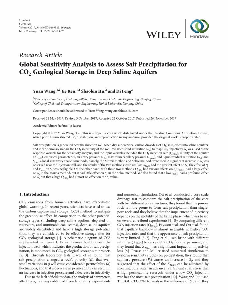
CO2 emissions from human activities have exacerbatedglobal warming. In recent years, scientists have tried to usethe carbon capture and storage (CCS) method to mitigatethe greenhouse effect. In comparison to the other potentialstorage types (including deep saline aquifers, depleted oilreservoirs, and unminable coal seams), deep saline aquifersare widely distributed and have a high storage potential;thus, they are considered to be effective storage sites forCO2 geological storage [1]. A schematic diagram of CCSis presented in Figure 1. Extra pressure buildup near theinjection well, which indicates the production of salt precip-itation, is monitored in CO2 geological storage site projects[2, 3]. Through laboratory tests, Bacci et al. found thatsalt precipitation changed a rock’s porosity (𝜙), that evensmall variations in 𝜙 will cause considerable permeability (𝑘)fluctuations, and that a decrease in permeability can result inan increase in injection pressure and a decrease in injectivity.

Due to the lack of field test data, the analysis of parametersaffecting 𝑆𝑠 is always obtained from laboratory experiments

and numerical simulation. Ott et al. conducted a core scaledrainage test to compare the salt precipitation of the corewith two different pore structures, they found that the porousrock is more prone to form salt precipitation than single-pore rock, and they believe that the impairment of injectivitydepends on the mobility of the brine phase, which was basedon several core flood experiments [4]. By comparing differentCO2 injection rates (𝑄CO2), Peysson et al. and Ott et al. foundthat capillary backflow is almost negligible at higher CO2injection rates and that the appearance of salt precipitationis very limited [5–7]. Tang et al. used brine with differentsalinities (𝑋NaCl) to carry out a CO2 flood experiment, andthey found that 𝑋NaCl has a significant impact on injectivityloss [8]. Pruess and Muller used numerical simulation toperform sensitivity studies on precipitation, they found thatcapillary pressure (𝑃𝑐) causes an increase in 𝑆𝑠, and theysuggested that the effect of the 𝑋NaCl can be alleviated byinjecting pure water in advance [9]. Guyant et al. stress thata high permeability reservoir under a low CO2 injectionrate has the most salt precipitation [10]. Wang and Liu usedTOUGH2/ECO2N to analyze the influence of 𝑆𝑠, and they

HindawiGeofluidsVolume 2017, Article ID 5603923, 16 pageshttps://doi.org/10.1155/2017/5603923

2 Geofluids

Injection well

compressionTransportation

pipeline

Deep saline aquifers

＃／2

＃／2 injection

＃／2 source

＃／2 capture

Figure 1: The process of CCS in deep saline aquifers.

found that 𝑆𝑠 will increase when 𝑄CO2 decreases, 𝑋NaClincreases, or 𝑃𝑐 increases [11, 12]. The results of the abovestudies are focused on local sensitivity analysis of a singlefactor and study 𝑆𝑠 with a single factor with specific changes;however, the global sensitivity evaluation of each factor hasnot yet been studied.

A global sensitivity analysis method can test the interac-tion between parameters, and it can test the effect of multipleparameters, which change concurrently on the responsevariable. The conventional approach to performing globalsensitivity analysis is the Morris sensitivity test method, theFourier amplitude sensitivity test (FAST), and the Sobolsensitivity test method [13–15]. Global sensitivity analysishas been widely used in hydrological models and designmodels [16, 17]. Global sensitivity analysis requires a largenumber of model calculations, and the salt precipitationmodel for geological storage is very complex; thus, it is verydifficult to calculate the global sensitivity of salt precipitation.Zheng et al. performed a sensitivity analysis of the CO2transport process in deep saline aquifers and comparedthe results of Morris, Sobol, and other global sensitivityanalysis methods, and they found that the sensitivity ordersof the input variables are different for different responsevariables and that the computational burden of the Sobolmethod is too large [18, 19]. Wainwright et al. performed asensitivity analysis using iTOUGH2 for CO2/brinemigrationand pressure buildup. Global sensitivity analysis of CO2sequestration always focuses on the distribution of CO2 andsite pressure changes, and these data are used for projectmonitoring; however, few studies have performed globalsensitivity analysis of the phenomenon of salt precipitation[20].

The traditional Sobol method extracts the parametersfirst, and then, it applies the parameters into a formula ormodel to calculate the response value. If a model has a clearmathematical formula, it is feasible to extract many samples,such as a polynomial model for the Sobol calculation basedon the experimental results [21]. However, physical modelsare often very complicated, and it is difficult to obtain a clearmathematical formula.

Zheng et al. selected parameters to calculate responsevariables based on the TOUGH2/ECO2N model, and theyfound when the number of samples is small, the sensitivitycoefficient may be negatively affected by the calculation; thusthe number of samples they used was 8129 [19]. The tradi-tional operation of the TOUGH2/ECO2N module consistsof four steps: modifying the input parameters, entering therun instructions, calculating, and viewing the output results.Each set of parameters is run once, and the computationalcomplexity of the Sobol sensitivity is too large. A surrogatemodel is an engineering method used when an outcome ofinterest cannot be directly measured; thus amodel of the out-come is used as an alternative. Zhang and Sahinidis used thesurrogatemodel from the polynomial chaos expansion (PCE)to conduct uncertainty analysis, but they mainly consideredthe uncertainty between the residual water saturation andthe injection rate [22]. Wu et al. proposed the use of Krigingsurrogate models for uncertainty and sensitivity analysis innuclear engineering [23]. Palar and Shimoyama used theKriging method to solve expensive multiobjective designoptimization problem [24]. Zhao et al. use Kriging surrogatemodel as an optimization approach for identifying the releasehistory of groundwater sources [25]. Hou et al. used thissurrogate model to conduct the sensitivity and uncertaintyanalysis [26], it is more precise and allows more samplingtimes to be calculated so that the results of the Sobol globalsensitivity analysis are more accurate.

In this paper, a simple radial flow model was established,and the numerical simulation of the salt precipitate modelwas performed by TOUGH2/ECO2N [12]. To analyze theglobal sensitivity of the salt precipitation, we chose 𝑆𝑠 as theresponse variable of the global sensitivity analysis method,which was one of the results of the numerical simulation.Input variables included the CO2 injection rate (𝑄CO2),salinity of the aquifer (𝑋NaCl), empirical parameter 𝑚, airentry pressure (𝑃0), maximum capillary pressure (𝑃max),liquid residual saturation in the relative permeability function(𝑆plr), and liquid residual saturation in the capillary pressurefunction (𝑆clr). The global sensitivity analysis was carried outby the Morris method and the Sobol method, which arequalitative and quantitative methods, respectively [13, 15].The impacts of each parameter and parameter combinationon 𝑆𝑠 were investigated. The Morris method could quicklyselect the insensitive parameters, and the number of samplesused in the calculation was small. The Sobol sensitivitymethod was more complicated to calculate, but it calculatedthe quantitative sensitivity and sensitivity orders of all thevariables.

Salt precipitation is always generated near the injectionwell when dry scCO2 is injected into deep saline aquifers,and it can seriously impair CO2 injectivity. The effect of saltprecipitation on the injectivity of a well is represented bysolid saturation (𝑆𝑠) near the injection well. It is necessaryto analyze the factors that affect the value of 𝑆𝑠 near theinjection well and then determine the main parametersand the negligible parameters that affect the 𝑆𝑠 value. Weused two global sensitivity analysis methods, and the mainmethod used in this paper was the Sobol global sensitivityanalysis method, which was used to determine the sensitivity

Geofluids 3

ΓL

L

R r

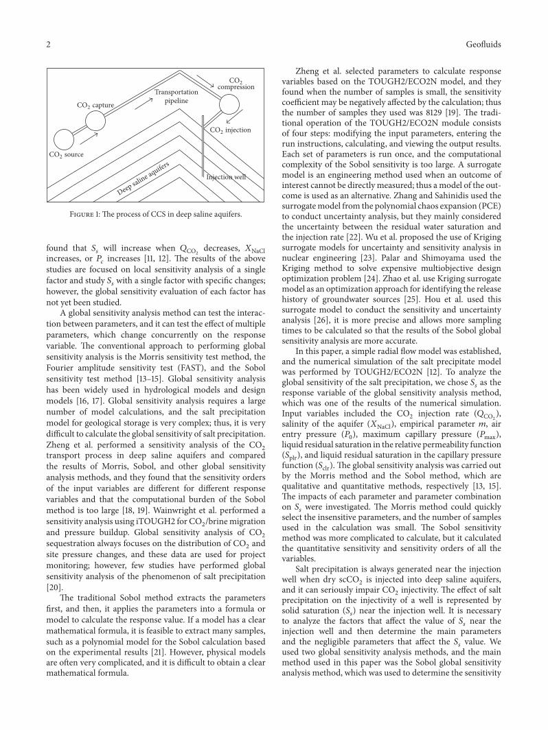
Figure 2: Tubes-in-series model (where 𝑅 is the radius of the coarsetube, 𝑟 is the radius of the thin tube, 𝐿 is the total length of a setof coarse and thin tubes, and Γ is the fractional length of the porebodies) [30].

orders of all the input variables [15]. The Kriging surrogatemodel was established to calculate the response variable 𝑆𝑠,and this model replaced the operation of TOUGH2/ECO2Nand reduced the simulation time to increase the efficiencyof the Sobol sensitivity analysis method [27]. The MonteCarlo algorithm was used to calculate the Sobol globalsensitivity values for all input parameters, and the MonteCarlo algorithm reduced the computation load and improvedthe calculation accuracy [28, 29].

2. Numerical Simulation of Salt Precipitation

The depth of a formation layer suitable for CO2 geologicalstorage is generally more than 800m; the temperature andthe pressure of the layer must exceed the critical valueof CO2 (31.1 centigrade and 7.38MPa, resp.). During theprocess of supercritical CO2 (scCO2) being injected intodeep saline aquifers, the scCO2 is considered a nonwettingphase and the brine is considered a wetting phase. If thenonwetting phase is injected into the wetting phase, the waterin the brine evaporates into the dry CO2 stream, and saltprecipitation is formed when the brine reaches its solubilitylimit. Accumulation of salt precipitation near the injectionwell blocks the CO2 flow path, resulting in a decrease in 𝑘near the injection well and reduced well injectivity.

Verma and Pruess provide a simple conceptual model tocharacterize the variation of 𝑘 with 𝑆𝑠 near the injection well[30]. These authors use a tubes-in-series model to simulatethe natural condition of porous media rock (Figure 2), andthey obtain the change in 𝑘 near the injection well with 𝑆𝑠according to the tubes-in-series model:

𝑘𝑘0 = 𝜃2 1 − Γ + Γ/𝜔2

1 − Γ + Γ [𝜃/ (𝜃 + 𝜔 − 1)]2 (1)

𝜃 = 1 − 𝑆𝑠 − 𝜙𝑟1 − 𝜙𝑟 (2)

𝜔 = 1 + 1/Γ1/𝜙𝑟 − 1 , (3)

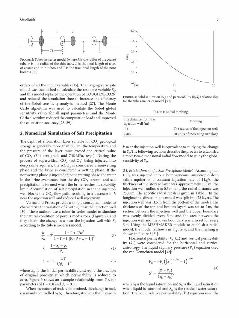
where 𝑘0 is the initial permeability and 𝜙𝑟 is the fractionof original porosity at which permeability is reduced tozero. Figure 3 shows an example relationship from (1), forparameters of Γ = 0.8 and 𝜙𝑟 = 0.8.

When the nature of rock is determined, the change in rock𝑘 is mainly controlled by 𝑆𝑠.Therefore, studying the change in

0.1 0.20.0Ss

0.0

0.2

0.4

0.6

0.8

1.0

k/k

0

Figure 3: Solid saturation (𝑆𝑠) and permeability (𝑘/𝑘0) relationshipfor the tubes-in-series model [30].

Table 1: Radial meshing.

The distance from theinjection well (m) Meshing

0.3 The radius of the injection well2500 50 units of increasing size (log)

𝑘 near the injection well is equivalent to studying the changein 𝑆𝑠.The following sections describe the process to establish asimple two-dimensional radial flowmodel to study the globalsensitivity of 𝑆𝑠.2.1. Establishment of a Salt Precipitate Model. Assuming thatCO2 was injected into a homogeneous, anisotropic deepsaline aquifer at a constant injection rate of 1 kg/s, thethickness of the storage layer was approximately 100m, theinjection well radius was 0.3m, and the radial distance was2500m. The specific radial mesh is given in Table 1. In thelongitudinal direction, the model was split into 22 layers.Theinjection well was 11.5m from the bottom of the model. Thethickness of the top and bottom layers was set to 2m, thesection between the injection well and the upper boundarywas evenly divided every 5m, and the area between theinjection well and the lower boundary was also set for every5m. Using the MESHMAKER module to establish a radialmodel, the model is shown in Figure 4, and the meshing isshown in Figure 5 [31].

Horizontal permeability (𝑘𝑥, 𝑘𝑦) and vertical permeabil-ity (𝑘𝑧) were considered for the horizontal and verticalanisotropy. The liquid capillary pressure (𝑃cl) equation usedthe van Genuchten model [32]:

𝑃cl = −𝑃0 ([𝑆∗]−1/𝑚 − 1)1−𝑚

𝑆∗ = (𝑆𝑙 − 𝑆lr)(𝑆ls − 𝑆lr) ,(4)

where 𝑆𝑙 is the liquid saturation and 𝑆ls is the liquid saturationwhen liquid is saturated and 𝑆lr is the residual water satura-tion. The liquid relative permeability (𝑘rl) equation used the

4 Geofluids

Table 2: The parameters of the radial model.

Parameter valueSaline aquifer 𝑘𝑥 = 100mD, 𝑘𝑦 = 100mD, 𝑘𝑧 = 20mD, 𝜙 = 12%

(Injection well) Initial condition (depth: −88.5m) Pressure (𝑃) = 12MPa, temperature (𝑇) = 45∘C, gas saturation (𝑆gas) = 0%,𝑋NaCl = 15%Boundary condition 𝑄CO2 = 1 kg/s, the upper and lower and right borders are no flow boundariesThe parameters in the relative permeability equation 𝑚 = 0.457, 𝑆lr = 0.30, 𝑆gr = 0.05, 𝑆ls = 1The parameters in the capillary pressure equation 𝑚 = 0.457, 𝑆lr = 0.30, 𝑃0 = 19.61 kPa, 𝑃max = 10MPa, 𝑆ls = 0.999

H = 100 m

h = 11.5 m R = 2500 m

r = 0.3 m

= 1 kg/sQ＃／2

Figure 4: Concept radial model (where 𝑅 is the radial distance, 𝑟 isthe radius of the injection well, ℎ is the distance from the injectionwell to the bottom, and𝐻 is the thickness of the storage layer).

No flow boundary

No

flow

bou

ndar

y

No flow boundary

−100

−80

−60

−40

−20

0

Elev

atio

n (m

)

500 1000 1500 2000 25000Distance (m)

Figure 5: Reservoir meshing diagram (the upper and lower bordersand right borders are sealed).

van Genuchten-Mualem model [32, 33], and the gas relativepermeability (𝑘rg) equation used Corey model [34]:

𝑘rl = √𝑆∗ {1 − (1 − [𝑆∗]1/𝑚)𝑚}2

𝑘rg = {{{1 − 𝑘rl if 𝑆gr = 0(1 − 𝑆)2 (1 − 𝑆2) if 𝑆gr > 0

𝑆 = (𝑆𝑙 − 𝑆lr)(𝑆ls − 𝑆lr − 𝑆gr) ,

(5)where 𝑆gr is the residual gas saturation. The parameters ofthe model are presented in Table 2. The plots of the capillarypressures and relative permeabilities are given in Figures 6and 7.

2.2. Results of theNumerical Simulation. TheECO2Nmodulewas used to simulate the migration of the CO2 in deep salineaquifers and obtain the value of 𝑆𝑔, 𝑆𝑠, and 𝑃. The time ofthe numerical simulation was set to 100 days, half a year, andone year. The results of the numerical simulation are given inFigures 8, 9, and 10.

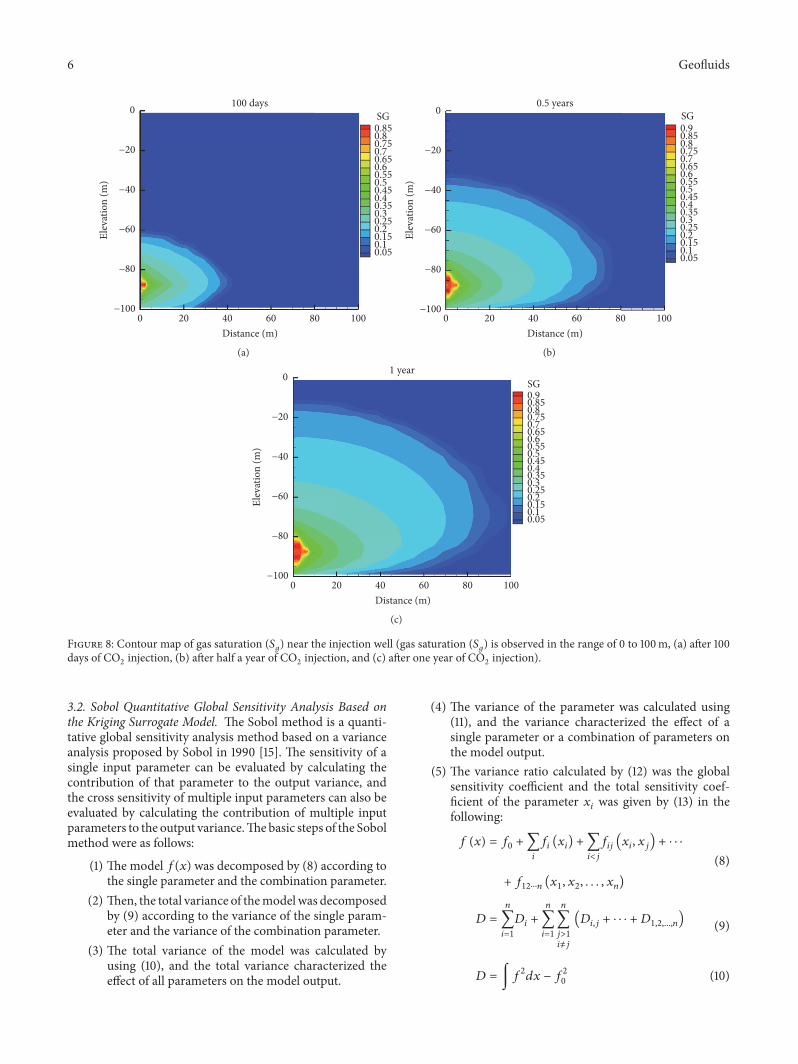
Figure 8 shows the contour map of 𝑆𝑔 near the injectionwell, and since the vapor content of the gas is small, the gassaturation can be approximated by the saturation of CO2.With the increase in time, CO2 migrates gradually and tendsto accumulate upward due to buoyancy. The 𝑆𝑔 value of theinjection well is approximately 0.9, and it is higher than inother areas. Figure 9 shows the contour map of 𝑆𝑠 near theinjection well. The value of 𝑆𝑠 near the injection well is thelargest, which indicates that the salt precipitates accumulatemainly near the well area. With the increase in the injectiontime, the range of salt precipitation gradually increases, andthe direction of the salt precipitate is consistent with the CO2flow. The values of 𝑆𝑠 and 𝑆𝑔 near the injection well almostreach the maximum value with the increase in time, and 𝑆𝑙near the injection well almost approaches zero, indicatingthat the injection well becomes a dry zone. The increase in𝑆𝑠 near the injection well means that the permeable pores arebeing blocked, which affects CO2 injectivity, causes pressurebuildup in the injection well, as shown in Figure 10, and mayincrease the risk of leakage during the CO2 injection process.

To assess the effect of salt precipitatemodel parameters oninjectivity, 𝑆𝑠 of the injectionwell was selected as the responsevariable, and the global sensitivity of the model parameterswas analyzed.

3. Global Sensitivity Analysis

3.1. Morris Qualitative Global Sensitivity Analysis. Morrisproposed a data screening method that can select parametersthat have a low impact on the results and reduce the numberof analysis variables [13]. In this paper, the Morris methodwas used to analyze the sensitivity of salt precipitate modelparameters, the range of parameters selected for the Morris

Geofluids 5

0.2 0.4 0.6 0.8 1.00.0

Sl

106

107

108

109

1010

P＝Ｆ(０

；)

Figure 6: Capillary pressure curve.

0.2 0.4 0.6 0.8 1.00.0

Sl

0.0

0.2

0.4

0.6

0.8

1.0

Rela

tive p

erm

eabi

lity

kＬＡ

kＬＦ

Figure 7: Relative permeability curve.

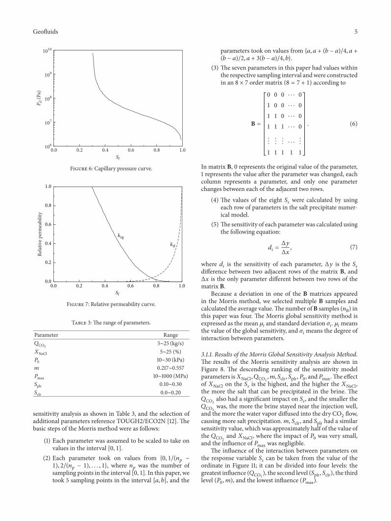
Table 3: The range of parameters.

Parameter Range𝑄CO2 5∼25 (kg/s)𝑋NaCl 5∼25 (%)𝑃0 10∼30 (kPa)𝑚 0.217∼0.557𝑃max 10∼1000 (MPa)𝑆plr 0.10∼0.30𝑆clr 0.0∼0.20

sensitivity analysis as shown in Table 3, and the selection ofadditional parameters reference TOUGH2/ECO2N [12]. Thebasic steps of the Morris method were as follows:

(1) Each parameter was assumed to be scaled to take onvalues in the interval [0, 1].

(2) Each parameter took on values from {0, 1/(𝑛𝑝 −1), 2/(𝑛𝑝 − 1), . . . , 1}, where 𝑛𝑝 was the number ofsampling points in the interval [0, 1]. In this paper, wetook 5 sampling points in the interval [𝑎, 𝑏], and the

parameters took on values from {𝑎, 𝑎 + (𝑏 − 𝑎)/4, 𝑎 +(𝑏 − 𝑎)/2, 𝑎 + 3(𝑏 − 𝑎)/4, 𝑏}.(3) The seven parameters in this paper had values within

the respective sampling interval andwere constructedin an 8 × 7 order matrix (8 = 7 + 1) according to

B =

[[[[[[[[[[[[[

0 0 0 ⋅ ⋅ ⋅ 01 0 0 ⋅ ⋅ ⋅ 01 1 0 ⋅ ⋅ ⋅ 01 1 1 ⋅ ⋅ ⋅ 0... ... ... ⋅ ⋅ ⋅ ...1 1 1 1 1

]]]]]]]]]]]]]

. (6)

In matrix B, 0 represents the original value of the parameter,1 represents the value after the parameter was changed, eachcolumn represents a parameter, and only one parameterchanges between each of the adjacent two rows.

(4) The values of the eight 𝑆𝑠 were calculated by usingeach row of parameters in the salt precipitate numer-ical model.

(5) The sensitivity of each parameter was calculated usingthe following equation:

𝑑𝑖 = Δ𝑦Δ𝑥 , (7)

where 𝑑𝑖 is the sensitivity of each parameter, Δ𝑦 is the 𝑆𝑠difference between two adjacent rows of the matrix B, andΔ𝑥 is the only parameter different between two rows of thematrix B.

Because a deviation in one of the B matrices appearedin the Morris method, we selected multiple B samples andcalculated the average value.The number ofB samples (𝑛𝐵) inthis paper was four. The Morris global sensitivity method isexpressed as the mean 𝜇𝑖 and standard deviation 𝜎𝑖. 𝜇𝑖 meansthe value of the global sensitivity, and 𝜎𝑖 means the degree ofinteraction between parameters.

3.1.1. Results of the Morris Global Sensitivity Analysis Method.The results of the Morris sensitivity analysis are shown inFigure 8. The descending ranking of the sensitivity modelparameters is𝑋NaCl,𝑄CO2 ,𝑚, 𝑆clr, 𝑆plr,𝑃0, and𝑃max.The effectof 𝑋NaCl on the 𝑆𝑠 is the highest, and the higher the 𝑋NaCl,the more the salt that can be precipitated in the brine. The𝑄CO2 also had a significant impact on 𝑆𝑠, and the smaller the𝑄CO2 was, the more the brine stayed near the injection well,and the more the water vapor diffused into the dry CO2 flow,causing more salt precipitation.𝑚, 𝑆clr, and 𝑆plr had a similarsensitivity value, which was approximately half of the value ofthe 𝑄CO2 and 𝑋NaCl, where the impact of 𝑃0 was very small,and the influence of 𝑃max was negligible.

The influence of the interaction between parameters onthe response variable 𝑆𝑠 can be taken from the value of theordinate in Figure 11; it can be divided into four levels: thegreatest influence (𝑄CO2), the second level (𝑆plr, 𝑆clr), the thirdlevel (𝑃0,𝑚), and the lowest influence (𝑃max).

6 Geofluids

0 20 40 60 80

Elev

atio

n (m

)0

−20

−40

−60

−80

−100100

Distance (m)

100 days

0.050.10.150.20.250.30.350.40.450.50.550.60.650.70.750.80.85SG

(a)

0 20 40 60 80

Elev

atio

n (m

)

0

−20

−40

−60

−80

−100100

Distance (m)

0.5 years

0.050.10.150.20.250.30.350.40.450.50.550.60.650.70.750.80.850.9SG

(b)

0 20 40 60 80

Elev

atio

n (m

)

0

−20

−40

−60

−80

−100100

Distance (m)

1 year

0.050.10.150.20.250.30.350.40.450.50.550.60.650.70.750.80.850.9SG

(c)

Figure 8: Contour map of gas saturation (𝑆𝑔) near the injection well (gas saturation (𝑆𝑔) is observed in the range of 0 to 100m, (a) after 100days of CO2 injection, (b) after half a year of CO2 injection, and (c) after one year of CO2 injection).

3.2. Sobol Quantitative Global Sensitivity Analysis Based onthe Kriging Surrogate Model. The Sobol method is a quanti-tative global sensitivity analysis method based on a varianceanalysis proposed by Sobol in 1990 [15]. The sensitivity of asingle input parameter can be evaluated by calculating thecontribution of that parameter to the output variance, andthe cross sensitivity of multiple input parameters can also beevaluated by calculating the contribution of multiple inputparameters to the output variance.Thebasic steps of the Sobolmethod were as follows:

(1) The model 𝑓(𝑥) was decomposed by (8) according tothe single parameter and the combination parameter.

(2) Then, the total variance of themodelwas decomposedby (9) according to the variance of the single param-eter and the variance of the combination parameter.

(3) The total variance of the model was calculated byusing (10), and the total variance characterized theeffect of all parameters on the model output.

(4) The variance of the parameter was calculated using(11), and the variance characterized the effect of asingle parameter or a combination of parameters onthe model output.

(5) The variance ratio calculated by (12) was the globalsensitivity coefficient and the total sensitivity coef-ficient of the parameter 𝑥𝑖 was given by (13) in thefollowing:

𝑓 (𝑥) = 𝑓0 + ∑𝑖

𝑓𝑖 (𝑥𝑖) + ∑𝑖<𝑗

𝑓𝑖𝑗 (𝑥𝑖, 𝑥𝑗) + ⋅ ⋅ ⋅+ 𝑓12⋅⋅⋅𝑛 (𝑥1, 𝑥2, . . . , 𝑥𝑛)

(8)

𝐷 = 𝑛∑𝑖=1

𝐷𝑖 +𝑛∑𝑖=1

𝑛∑𝑗>1𝑖 =𝑗

(𝐷𝑖,𝑗 + ⋅ ⋅ ⋅ + 𝐷1,2,...,𝑛) (9)

𝐷 = ∫𝑓2𝑑𝑥 − 𝑓20 (10)

Geofluids 7

0 2 4 6 8

Elev

atio

n (m

)0

−20

−40

−60

−80

−10010

Distance (m)

100 days

0.020.010.030.040.050.060.070.080.090.10.110.120.130.140.150.160.170.18SS

(a)

0 2 4 6 8

Elev

atio

n (m

)

0

−20

−40

−60

−80

−10010

Distance (m)

0.5 years

0.020.010.030.040.050.060.070.080.090.10.110.120.130.140.150.160.170.18SS

(b)

0 2 4 6 8

Elev

atio

n (m

)

0

−20

−40

−60

−80

−10010

Distance (m)

1 year

0.020.010.030.040.050.060.070.080.090.10.110.120.130.140.150.160.170.18SS

(c)

Figure 9: Contour map of solid saturation (𝑆𝑠) near the injection well (solid saturation (𝑆𝑠) is observed in the range of 0 to 10m, (a) after 100days of CO2 injection, (b) after half a year of CO2 injection, and (c) after one year of CO2 injection).

𝐷𝑖1 ⋅⋅⋅𝑖𝑠 = ∫𝑓2𝑖1 ⋅⋅⋅𝑖𝑠𝑑𝑥𝑖1 ⋅ ⋅ ⋅ 𝑑𝑥𝑖𝑠 (11)

𝑆𝑖1 ⋅⋅⋅𝑖𝑠 = 𝐷𝑖1 ⋅⋅⋅𝑖𝑠𝐷 (12)

𝑆𝑇𝑖 = (𝐷 − 𝐷−𝑖)𝐷 , (13)

where 𝑆𝑖1 is the first-order sensitivity coefficient, and thiscoefficient described the contribution of the independenteffect of the parameter on the sensitivity. 𝑆𝑖1𝑖2 is the second-order sensitivity coefficient, which describes the contributionof the parameter interaction to the sensitivity. 𝑆𝑇1 is the totalsensitivity coefficient, and this coefficient is the sum of everystep of sensitivity coefficients of the parameter. In (13), 𝐷−𝑖characterizes the effect on variancewith all parameters except𝑥𝑖 and their interaction.

If the model has a clear mathematical expression 𝑓(𝑥),Sobol sensitivity can be calculated from (12) and (13), but if

the model does not have a clear mathematical expression,the sensitivity is calculated by the Monte Carlo method[29, 35]. In this paper, we used the Monte Carlo methodto calculate the Sobol sensitivity because it was difficult toestablish a definite mathematical expression for 𝑆𝑠. If thenumber of samples is too low, then the sensitivity coefficientwould be negative. The Sobol sensitivity calculation usuallyhas two drawbacks: the input parameters and the runningtime of the model. If the number of samples is too small,then the sensitivity coefficient would be negative. To reducethe computational load while sampling a large number ofsamples, a surrogate model was proposed instead of the saltprecipitate model in TOUGH2/ECO2N to calculate 𝑆𝑠. Thesurrogatemodel was amathematicalmodel that, by fitting thediscrete data, could help to predict the output of the physicalmodel.

3.2.1. Kriging Surrogate Model and the Monte Carlo Method.The Kriging surrogate model is a semiparametric model

8 Geofluids

0 2 4 6 8

Elev

atio

n (m

)

0

−20

−40

−60

−80

−10010

Distance (m)

100 days

1.12E + 071.13E + 071.14E + 071.15E + 071.16E + 071.17E + 071.18E + 071.19E + 071.20E + 071.21E + 071.22E + 071.23E + 071.24E + 071.25E + 071.26E + 071.27E + 07

P (Pa)

(a)

0 2 4 6 8

Elev

atio

n (m

)

0

−20

−40

−60

−80

−10010

Distance (m)

0.5 years

1.13E + 071.14E + 071.15E + 071.16E + 071.17E + 071.18E + 071.19E + 071.2E + 071.21E + 071.22E + 071.23E + 071.24E + 071.25E + 071.26E + 07

P (Pa)

(b)

0 2 4 6 8

Elev

atio

n (m

)

0

−20

−40

−60

−80

−10010

Distance (m)

1 year

1.14E + 071.15E + 071.16E + 071.17E + 071.18E + 071.19E + 071.2E + 071.21E + 071.22E + 071.23E + 071.24E + 071.25E + 071.26E + 071.27E + 07

P (Pa)

(c)

Figure 10: Contour map of fluid pressure (𝑃) near the injection well (pressure (𝑃) is observed in the range of 0 to 10m, (a) after 100 days ofCO2 injection, (b) after half a year of CO2 injection, and (c) after one year of CO2 injection).

Geofluids 9

0.00

0.05

0.10

i

0.02 0.04 0.06 0.08 0.100.00i

X．；＃Ｆ

S＝ＦＬSＪＦＬ

PＧ；Ｒ

P0 m

Q＃／2

Figure 11: Morris global sensitivity analysis of 𝑆𝑠 near the injectionwell.

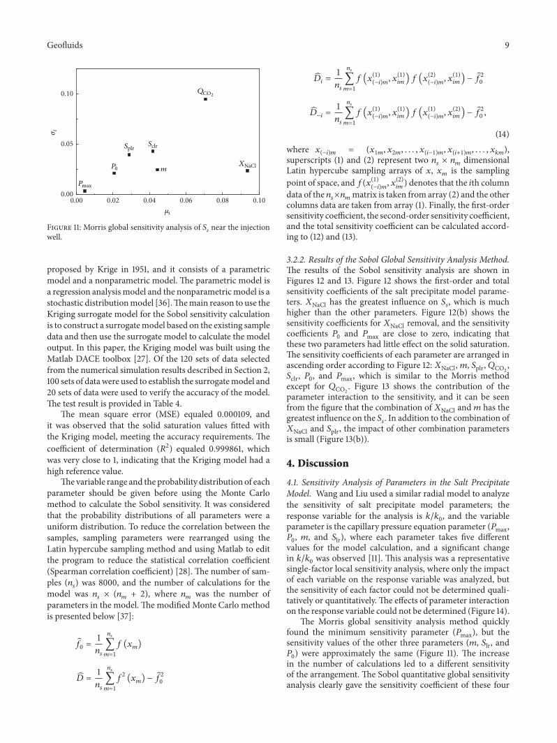
proposed by Krige in 1951, and it consists of a parametricmodel and a nonparametric model. The parametric model isa regression analysis model and the nonparametricmodel is astochastic distributionmodel [36].Themain reason to use theKriging surrogate model for the Sobol sensitivity calculationis to construct a surrogatemodel based on the existing sampledata and then use the surrogate model to calculate the modeloutput. In this paper, the Kriging model was built using theMatlab DACE toolbox [27]. Of the 120 sets of data selectedfrom the numerical simulation results described in Section 2,100 sets of datawere used to establish the surrogatemodel and20 sets of data were used to verify the accuracy of the model.The test result is provided in Table 4.

The mean square error (MSE) equaled 0.000109, andit was observed that the solid saturation values fitted withthe Kriging model, meeting the accuracy requirements. Thecoefficient of determination (𝑅2) equaled 0.999861, whichwas very close to 1, indicating that the Kriging model had ahigh reference value.

The variable range and the probability distribution of eachparameter should be given before using the Monte Carlomethod to calculate the Sobol sensitivity. It was consideredthat the probability distributions of all parameters were auniform distribution. To reduce the correlation between thesamples, sampling parameters were rearranged using theLatin hypercube sampling method and using Matlab to editthe program to reduce the statistical correlation coefficient(Spearman correlation coefficient) [28]. The number of sam-ples (𝑛𝑠) was 8000, and the number of calculations for themodel was 𝑛𝑠 × (𝑛𝑚 + 2), where 𝑛𝑚 was the number ofparameters in the model. The modified Monte Carlo methodis presented below [37]:

𝑓0 = 1𝑛𝑠𝑛𝑠∑𝑚=1

𝑓 (𝑥𝑚)

𝐷 = 1𝑛𝑠𝑛𝑠∑𝑚=1

𝑓2 (𝑥𝑚) − 𝑓20

𝐷𝑖 = 1𝑛𝑠𝑛𝑠∑𝑚=1

𝑓 (𝑥(1)(−𝑖)𝑚, 𝑥(1)𝑖𝑚 ) 𝑓 (𝑥(2)(−𝑖)𝑚, 𝑥(1)𝑖𝑚 ) − 𝑓20

𝐷−𝑖 = 1𝑛𝑠𝑛𝑠∑𝑚=1

𝑓 (𝑥(1)(−𝑖)𝑚, 𝑥(1)𝑖𝑚 ) 𝑓 (𝑥(1)(−𝑖)𝑚, 𝑥(2)𝑖𝑚 ) − 𝑓20 ,(14)

where 𝑥(−𝑖)𝑚 = (𝑥1𝑚, 𝑥2𝑚, . . . , 𝑥(𝑖−1)𝑚, 𝑥(𝑖+1)𝑚, . . . , 𝑥𝑘𝑚),superscripts (1) and (2) represent two 𝑛𝑠 × 𝑛𝑚 dimensionalLatin hypercube sampling arrays of 𝑥, 𝑥𝑚 is the samplingpoint of space, and𝑓(𝑥(1)

(−𝑖)𝑚, 𝑥(2)𝑖𝑚 ) denotes that the 𝑖th column

data of the 𝑛𝑠×𝑛𝑚matrix is taken from array (2) and the othercolumns data are taken from array (1). Finally, the first-ordersensitivity coefficient, the second-order sensitivity coefficient,and the total sensitivity coefficient can be calculated accord-ing to (12) and (13).

3.2.2. Results of the Sobol Global Sensitivity Analysis Method.The results of the Sobol sensitivity analysis are shown inFigures 12 and 13. Figure 12 shows the first-order and totalsensitivity coefficients of the salt precipitate model parame-ters. 𝑋NaCl has the greatest influence on 𝑆𝑠, which is muchhigher than the other parameters. Figure 12(b) shows thesensitivity coefficients for 𝑋NaCl removal, and the sensitivitycoefficients 𝑃0 and 𝑃max are close to zero, indicating thatthese two parameters had little effect on the solid saturation.The sensitivity coefficients of each parameter are arranged inascending order according to Figure 12: 𝑋NaCl, 𝑚, 𝑆plr, 𝑄CO2 ,𝑆clr, 𝑃0, and 𝑃max, which is similar to the Morris methodexcept for 𝑄CO2 . Figure 13 shows the contribution of theparameter interaction to the sensitivity, and it can be seenfrom the figure that the combination of 𝑋NaCl and 𝑚 has thegreatest influence on the 𝑆𝑠. In addition to the combination of𝑋NaCl and 𝑆plr, the impact of other combination parametersis small (Figure 13(b)).

4. Discussion

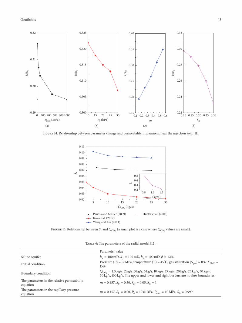
4.1. Sensitivity Analysis of Parameters in the Salt PrecipitateModel. Wang and Liu used a similar radial model to analyzethe sensitivity of salt precipitate model parameters; theresponse variable for the analysis is 𝑘/𝑘0, and the variableparameter is the capillary pressure equation parameter (𝑃max,𝑃0, 𝑚, and 𝑆lr), where each parameter takes five differentvalues for the model calculation, and a significant changein 𝑘/𝑘0 was observed [11]. This analysis was a representativesingle-factor local sensitivity analysis, where only the impactof each variable on the response variable was analyzed, butthe sensitivity of each factor could not be determined quali-tatively or quantitatively. The effects of parameter interactionon the response variable could not be determined (Figure 14).

The Morris global sensitivity analysis method quicklyfound the minimum sensitivity parameter (𝑃max), but thesensitivity values of the other three parameters (𝑚, 𝑆lr, and𝑃0) were approximately the same (Figure 11). The increasein the number of calculations led to a different sensitivityof the arrangement. The Sobol quantitative global sensitivityanalysis clearly gave the sensitivity coefficient of these four

10 Geofluids

Table4:Com

paris

onbetweenthep

redicted

valueo

fthe

Krigingmod

elandthec

alculated

values

ofthes

altp

recipitatemod

elin

Section2.

Seria

lnum

ber

𝑄 CO2(kg/s)

𝑋 NaCl(%

)𝑃 0(

kPa)

𝑚𝑃 ma

x(M

Pa)

𝑆 plr𝑆 clr

Predictedvalue(Kr

igingmod

el)

Calculated

value(saltprecipitatemod

el)

Relativee

rror

121

1018

0.221

6020.25

0.140.03

550.03

550.00

0959

212

727

0.303

7900.27

0.120.02

240.02

19−0.

002441

322

1721

0.411

6870.20

0.030.05

110.05

1−0.

00108

422

1227

0.219

8810.20

0.150.04

250.04

23−0.

00363

56

629

0.227

6170.15

0.070.01

950.01

950.00

2107

623

1013

0.510

7200.15

0.010.02

390.02

38−0.

00435

719

619

0.240

3580.30

0.170.02

060.02

01−0.

02536

89

1312

0.525

9890.27

0.140.03

610.03

640.00

8394

914

2024

0.504

4940.16

0.050.05

410.05

410.00

1852

106

2426

0.419

1170.26

0.180.08

050.08

050.00

2204

1122

2112

0.350

9210.24

0.010.07

180.07

190.00

0835

1221

2213

0.272

410.14

0.110.07

760.07

75−0.

000851

1322

2011

0.230

9280.16

0.090.07

360.07

35−0.

002023

1412

2126

0.455

2980.10

0.100.05

670.05

720.00

8249

1515

1618

0.480

7330.17

0.040.04

290.04

29−0.

000489

1618

1628

0.396

1180.11

0.180.04

470.04

46−0.

002059

177

1528

0.470

8480.18

0.190.04

070.04

06−0.

002457

1813

524

0.465

9110.14

0.010.01

190.01

220.02

6850

1923

1422

0.245

1130.20

0.160.04

890.04

88−0.

002025

2023

2320

0.456

3670.27

0.070.07

460.07

44−0.

002975

Geofluids 11

X．；＃Ｆ P0 SＪＦＬPＧ；Ｒ S＝ＦＬm

Model parameters (including X．；＃Ｆ)

First-order sensitivityTotal sensitivity

0.0

0.2

0.4

0.6

0.8

1.0Se

nsiti

vity

coeffi

cien

t

Q＃／2

(a)

Model parameters (excluding X．；＃Ｆ)

P0 SＪＦＬPＧ；Ｒ S＝ＦＬm

First-order sensitivityTotal sensitivity

0.00

0.01

0.02

0.03

0.04

0.05

0.06

0.07

Sens

itivi

ty co

effici

ent

Q＃／2

(b)

Figure 12: First-order and total sensitivity coefficients of salt precipitate model ((a) contain all the parameters, and (b) removes the mostinfluential parameters (𝑋NaCl)).

parameters, from large to small 𝑚, 𝑆lr, 𝑃0, and 𝑃max, wherethe sensitivity coefficient of 𝑃0 and 𝑃max was close to zero(Figure 12). For the interaction between the parameters,both methods showed that the interaction between thesefour parameters and other parameters had little effect onthe response variable. For large-scale and longtime saltprecipitate numerical simulations, it was feasible to set𝑃0 and𝑃max as empirical constants.

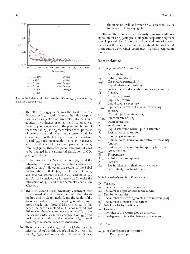
4.2. Effect of the CO2 Injection Rate on Solid Saturation. Manyresearchers have studied the effect of𝑄CO2 on 𝑆𝑠 by numericalsimulation; they consider that an increase in 𝑄CO2 decreasesthe 𝑆𝑠, and their results are shown in Figure 15 [9, 38–40].TheMorris method and Sobol method give a different sensitivityarrangement for 𝑄CO2 . In the Morris method, 𝑄CO2 is one ofthe main factors causing the change in 𝑆𝑠, which is consistentwith the conclusion of Pruess et al. [9, 38–40]. However, inthe Sobol method, the influence of the 𝑄CO2 on 𝑆𝑠 is muchsmaller than that of𝑋NaCl,𝑚, and 𝑆lr.

To study the effect of 𝑄CO2 on 𝑆𝑠 near the well, we chosemore𝑄CO2 values for the numerical simulation (ranging froma low injection rate of 1.5 kg/s to a high injection rate of100 kg/s). We modified the injection model by enlarging theradius of the model and refined the mesh near the injectionwell to set up a wide range of 𝑄CO2 . This paper referred to aTOUGH2/ECO2N case to divide the grid and set the modelparameters (Tables 5 and 6) [12]. We selected 11 different𝑄CO2 values for the simulation, and the results are shown inFigure 16.

Figure 16 shows the relationship between different valuesof 𝑄CO2 and 𝑆𝑠 near the injection well. The range of saltprecipitation increases with the increase in 𝑄CO2 . The valuesof 𝑆𝑠 at the injection well decrease with the increase in 𝑄CO2 ,and at a low𝑄CO2 , the brine in the unit near the injection wellevaporates more completely. In the low𝑄CO2 range (1.5 kg/s∼15 kg/s), it is clear that 𝑆𝑠 near the injectionwell decreaseswith

Table 5: 2D radial meshing [12].

The distance from the injectionwell (m) Meshing

0.3 The radius of the injection well103 200 units of increasing size (log)3 × 103 100 units of increasing size (log)104 100 units of increasing size (log)105 34 units of increasing size (log)

increasing 𝑄CO2 , which is consistent with the conclusions ofPruess et al. This finding is also consistent with the resultsof the Morris method (𝑄CO2 has considerable influence on𝑆𝑠) [9, 38–40]. However, in the high 𝑄CO2 range (15 kg/s∼100 kg/s), the value of 𝑆𝑠 near the injectionwell generally doesnot change. The variation in 𝑆𝑠 under high values of 𝑄CO2was not investigated in the previous sensitivity analysis of saltprecipitation [9, 38–40].

It was important to distinguish between 𝑆𝑠 at the injectionwell and 𝑆𝑠 near the injection well; the injection well wasa boundary condition, and its 𝑆𝑠 value could be inaccurate.The response variable for the sensitivity analysis was 𝑆𝑠 nearthe injection well. If the value of 𝑄CO2 was small, then theeffect of 𝑄CO2 on 𝑆𝑠 near the well was significant. If the valueof 𝑄CO2 was large, then the influence of 𝑄CO2 on 𝑆𝑠 nearthe well was negligible. This conclusion also explained thedifference between theMorris and Sobol results. In this paper,the range of 𝑄CO2 was 5 kg/s∼25 kg/s, the sampling numberand the sampling frequency of Morris method were small (4in this paper), most of the 𝑄CO2 values (75% in this paper)were in the low range, and the effect of 𝑄CO2 on 𝑆𝑠 near thewell was significant (Figure 11). However, the Sobol methodrequired a large sampling number (8192 in this paper) tocalculate the sensitivity coefficient, the selected 𝑄CO2 values

12 Geofluids

Model parameters interaction (including X．；＃Ｆ&m)

&X

．；＃

Ｆ

&P0

&m

&PＧ；Ｒ

&S Ｊ

ＦＬ

&S ＝

ＦＬ

X．；＃

Ｆ&P0

X．；＃

Ｆ&m

X．；＃

Ｆ&PＧ；Ｒ

X．；＃

Ｆ&S Ｊ

ＦＬ

X．；＃

Ｆ&S ＝

ＦＬ

P0&m

P0&PＧ；Ｒ

P0&S Ｊ

ＦＬ

P0&S ＝

ＦＬ

m&PＧ；Ｒ

m&S Ｊ

ＦＬ

m&S ＝

ＦＬ

PＧ；Ｒ

&S Ｊ

ＦＬ

PＧ；Ｒ

&S ＝

ＦＬ

S ＪＦＬ

&S ＝

ＦＬ

0.002

0.004

0.006

0.008

0.010

0.012

0.014

0.016

Seco

nd-o

rder

sens

itivi

ty

Q＃／

2 Q＃／

2

Q＃／

2

Q＃／

2

Q＃／

2

Q＃／

2

(a)

X．；＃Ｆ&m)Model parameters interaction (excludeing

&X

．；＃

Ｆ

&P0

&m

&PＧ；Ｒ

&S Ｊ

ＦＬ

&S ＝

ＦＬ

X．；＃

Ｆ&P0

X．；＃

Ｆ&PＧ；Ｒ

X．；＃

Ｆ&S Ｊ

ＦＬ

X．；＃

Ｆ&S ＝

ＦＬ

P0&m

P0&PＧ；Ｒ

P0&S Ｊ

ＦＬ

P0&S ＝

ＦＬ

m&PＧ；Ｒ

m&S Ｊ

ＦＬ

m&S ＝

ＦＬ

PＧ；Ｒ

&S Ｊ

ＦＬ

PＧ；Ｒ

&S ＝

ＦＬ

S ＪＦＬ

&S ＝

ＦＬ

0.0000

0.0005

0.0010

0.0015

0.0020

0.0025

0.0030

0.0035

0.0040

Seco

nd-o

rder

sens

itivi

ty

Q＃／

2 Q＃／

2

Q＃／

2

Q＃／

2

Q＃／

2

Q＃／

2

(b)

Figure 13: Second-order sensitivity coefficients of salt precipitate model ((a) contains all the parameter combinations, and (b) removes themost influential parameter combination (𝑋NaCl and𝑚)).

were uniform, and the effect of 𝑄CO2 on the 𝑆𝑠 was notsignificant (Figure 12(b)).

5. Conclusions

The radial model was used to simulate the salt precipitatenear the injection well during CO2 injection into deepsaline aquifers. Numerical simulation results showed that

evaporation led to salt precipitate near the injection well. Theincrease in 𝑆𝑠 reduced the injectivity and led to extra pressurebuildup near the injection well. In this paper, 𝑆𝑠 of the unitnear the injection well was selected as the response variable.The Morris global sensitivity analysis and the Sobol globalsensitivity analysis based on the Kriging surrogate modelwere carried out and themain conclusions obtained from thisstudy were as follows:

Geofluids 13

0.29

0.30

0.31

0.32

k/k

0

200 400 600 800 10000PＧ；Ｒ (－０；)

(a)

15 20 25 3010P0 (Ｅ０；)

0.300

0.305

0.310

0.315

0.320

0.325

k/k

0

(b)

0.2 0.3 0.4 0.5 0.60.1m

0.15

0.20

0.25

0.30

0.35

0.40

k/k

0(c)

0.15 0.20 0.25 0.300.10SＦＬ

0.22

0.24

0.26

0.28

0.30

0.32

k/k

0

(d)

Figure 14: Relationship between parameter change and permeability impairment near the injection well [11].

Hurter et al. (2008)

0.02

0.03

0.04

0.05

0.06

0.07

0.08

0.09

0.10

0.11

S s

0.20.40.60.8

S s

1.0 1.20.8

1510 20 25 305(ＥＡ/Ｍ)

(ＥＡ/Ｍ)

Kim et al. (2012)Wang and Liu (2014)

(2009)０ＬＯ？ＭＭ ；Ｈ＞－ＯＦＦ？Ｌ

Q＃／2

Q＃／2

Figure 15: Relationship between 𝑆𝑠 and 𝑄CO2 (a small plot is a case where 𝑄CO2 values are small).

Table 6: The parameters of the radial model [12].

Parameter valueSaline aquifer 𝑘𝑥 = 100mD, 𝑘𝑦 = 100mD, 𝑘𝑧 = 100mD, 𝜙 = 12%Initial condition Pressure (𝑃) = 12MPa, temperature (𝑇) = 45∘C, gas saturation (𝑆gas) = 0%,𝑋NaCl =

15%

Boundary condition 𝑄CO2 = 1.5 kg/s, 2 kg/s, 3 kg/s, 5 kg/s, 10 kg/s, 15 kg/s, 20 kg/s, 25 kg/s, 30 kg/s,50 kg/s, 100 kg/s. The upper and lower and right borders are no flow boundaries

The parameters in the relative permeabilityequation 𝑚 = 0.457, 𝑆lr = 0.30, 𝑆gr = 0.05, 𝑆ls = 1The parameters in the capillary pressureequation 𝑚 = 0.457, 𝑆lr = 0.00, 𝑃0 = 19.61 kPa, 𝑃max = 10MPa, 𝑆ls = 0.999

14 Geofluids

1.5 kg/s2 kg/s3 kg/s5 kg/s10 kg/s15 kg/s

20 kg/s25 kg/s30 kg/s50 kg/s100 kg/s

1 year

0.05

0.10

0.15

0.20

S s

10 20 30 40 50 60 70 80 90 1000Distance (m)

Figure 16: Relationships between the different 𝑄CO2 values and 𝑆𝑠near the injection well.

(i) The effect of 𝑋NaCl on 𝑆𝑠 was the greatest, and adecrease in 𝑋NaCl could decrease the salt precipita-tion, such as injection of pure water into the salineaquifer. The influence of 𝑚, 𝑆plr, and 𝑆clr on 𝑆𝑠 wassecondary: 𝑚 was related to the pore distribution ofthe formation, 𝑆plr and 𝑆clrwere related to the pore sizeof the formation, and these three parameters could becharacterized as the heterogeneity of the formation.𝑃0 and 𝑃max had similar results in sensitivity analysis,and the influence of these two parameters on 𝑆𝑠were negligible. These two parameters did not needto be changed in the numerical simulation of CO2geological storage.

(ii) In the results of the Morris method, 𝑄CO2 and theinteraction with other parameters had considerableinfluence on 𝑆𝑠. However, the results of the Sobolmethod showed that 𝑄CO2 had little effect on 𝑆𝑠and that the interactions of 𝑋NaCl and 𝑚, 𝑋NaCl,and 𝑆plr had considerable influence on 𝑆𝑠, while theinteraction of 𝑄CO2 and other parameters had a loweffect on 𝑆𝑠.

(iii) The high second-order sensitivity coefficient mayhave caused the difference between the Morrismethod and the Sobol method, and the results of theSobol method, with more sampling numbers, weremore reliable than those of Morris method. In thispaper, the Morris method and Sobol method haddifferent results related to the sensitivity of 𝑄CO2 , butthe second-order sensitivity coefficient of 𝑄CO2 wasnot large, which indicated that the effect of𝑄CO2 couldnot simply be characterized by sensitivity.

(iv) There was a critical 𝑄CO2 value (𝑄𝑐) during CO2injection (15 kg/s in this paper); when 𝑄CO2 was lessthan 𝑄𝑐, 𝑄CO2 had considerable influence on 𝑆𝑠 near

the injection well, and when 𝑄CO2 exceeded 𝑄𝑐, itsinfluence could be negligible.

The results of global sensitivity analysis to assess salt pre-cipitation for CO2 geological storage in deep saline aquifersprovide possible help for future field text and numerical sim-ulations. Salt precipitation mechanism should be consideredin the future work, which could affect the salt precipitationmodel.

Nomenclature

Salt Precipitate Model Parameters

𝑘: Permeability𝑘0: Initial permeability𝑘rg: Gas relative permeability𝑘rl: Liquid relative permeability𝑚: Formation pore distribution empirical parameter𝑃: Pressure𝑃0: Air entry pressure𝑃𝑐: Capillary pressure𝑃cl: Liquid capillary pressure𝑃max: Input absolute value of maximum capillarypressure𝑄𝑐: Critical injection rate of CO2𝑄CO2 : Injection rate of CO2𝑆𝑙: Water saturation𝑆𝑠: Solid saturation𝑆ls: Liquid saturation when liquid is saturated𝑆lr: Residual water saturation𝑆gr: Residual gas saturation𝑆plr: Residual water saturation in relative permeabilityfunction𝑆clr: Residual water saturation in capillary function𝑆gas: Gas saturation𝑇: Temperature𝑋NaCl: Salinity of saline aquifers𝜙: Porosity𝜙𝑟: The fraction of original porosity at whichpermeability is reduced to zero.

Global Sensitivity Analysis Parameters

𝐷𝑖: Variance𝑑𝑖: The sensitivity of each parameter𝑛𝑚: The number of parameters in the model𝑛𝑠: Number of samples𝑛𝑝: The number of sampling points in the interval [𝑎, 𝑏]𝑛𝐵: The number of matrix B selections𝑆𝑖: Sobol sensitivity coefficient𝑥𝑖: Parameter𝜇𝑖: The value of the Morris global sensitivity𝜎𝑖: The degree of interaction between parameters.

Subscripts

𝑥, 𝑦, 𝑧: Coordinate axis direction𝑖: Parameter type.

Geofluids 15

Conflicts of Interest

The authors declare that there are no conflicts of interestregarding the publication of this paper.

Acknowledgments

The research was supported by the National Natural ScienceFoundation of China (no. 51179060), the Education MinistryFoundation of China (no. 20110094130002), the FundamentalResearch Funds for theCentral Universities (no. 2015B26514),the Postgraduate Research & Practice Innovation Programof Jiangsu Province (no. KYCX17 0470), and the Funda-mental Research Funds for the Central Universities (no.2017B648X14).

References

[1] S. M. Benson and F. M. Orr, “Carbon Dioxide Capture andStorage,”MRS Bulletin, vol. 33, no. 04, pp. 303–305, 2005.

[2] G. Baumann, J. Henninges, and M. De Lucia, “Monitoring ofsaturation changes and salt precipitation during CO2 injectionusing pulsed neutron-gamma logging at the Ketzin pilot site,”International Journal of Greenhouse Gas Control, vol. 28, pp.134–146, 2014.

[3] S. Grude, M. Landrø, and J. Dvorkin, “Pressure effects causedby CO2 injection in the Tubaen Fm., the Snøhvit field,” Inter-national Journal of Greenhouse Gas Control, vol. 27, pp. 178–187,2014.

[4] H. Ott, J. Snippe, K. De Kloe, H. Husain, and A. Abri, “Salt pre-cipitation due to sc-gas injection: Single versus multi-porosityrocks,” in Proceedings of the 11th International Conference onGreenhouse Gas Control Technologies (GHGT ’12), pp. 3319–3330, Japan, November 2012.

[5] F. Peysson, “Permeability alteration induced by drying of brinesin porous media,” EPJ Applied Physics, vol. 60, no. 2, pp. 367–369, 2012.

[6] Y. Peysson, L. Andre, and M. Azaroual, “Well injectivityduring CO2 storage operations in deep saline aquifers-Part 1:Experimental investigation of drying effects, salt precipitationand capillary forces,” International Journal of Greenhouse GasControl, vol. 22, pp. 291–300, 2014.

[7] H. Ott, S. M. Roels, and K. de Kloe, “Salt precipitation due tosupercritical gas injection: I. Capillary-driven flow in unimodalsandstone,” International Journal of Greenhouse Gas Control,vol. 43, pp. 247–255, 2015.

[8] Y. Tang, R. Yang, Z. Du, and F. Zeng, “Experimental study offormation damage caused by complete water vaporization andsalt precipitation in sandstone reservoirs,” Transport in PorousMedia, vol. 107, no. 1, pp. 205–218, 2015.

[9] K. Pruess and N. Muller, “Formation dry-out from CO2injection into saline aquifers: 1. effects of solids precipitationand their mitigation,” Water Resources Research, vol. 45, no. 3,Article IDW03402, 2009.

[10] E. Guyant, W. S. Han, K.-Y. Kim, M.-H. Park, and B.-Y.Kim, “Salt precipitation and CO2/brine flow distribution underdifferent injection well completions,” International Journal ofGreenhouse Gas Control, vol. 37, pp. 299–310, 2015.

[11] Y.Wang and Y. Liu, “Impact of capillary pressure on permeabil-ity impairment during CO2 injection into deep saline aquifers,”

Journal of Central SouthUniversity, vol. 20, no. 8, pp. 2293–2298,2013.

[12] K. Pruess, ECO2N: a TOUGH2 Fluid property module formixtures of water, NaCl, and CO2, Earth Science Division,Lawrence Berkeley National Laboratory, 2005.

[13] M.D.Morris, “Factorial sampling plans for preliminary compu-tational experiments,” Technometrics, vol. 33, no. 2, pp. 161–174,1991.

[14] R. I. Cukier, C.M. Fortuin, K. E. Shuler, A. G. Petschek, and J. H.Schaibly, “Study of the sensitivity of coupled reaction systemsto uncertainties in rate coefficients. I Theory,” The Journal ofChemical Physics, vol. 59, no. 8, pp. 3873–3878, 1973.

[15] I. M. Sobol, “Sensitivity estimates for nonlinear mathematicalmodels,” Mathematical Modelling and Computational Experi-ments, vol. 1, no. 4, pp. 407–414, 1993.

[16] C. Tong, “Self-validated variance-based methods for sensitivityanalysis of model outputs,” Reliability Engineering & SystemSafety, vol. 95, no. 3, pp. 301–309, 2010.

[17] H. C. Frey and S. R. Patil, “Identification and review ofsensitivity analysis methods,” Risk Analysis, vol. 22, no. 3, pp.553–578, 2002.

[18] Z. Fei, S. Xiaoqing, and W. Jichun, “Global sensitivity analysisof leakage risk for CO2 geological sequestration in the salineaquifer of yancheng formation in subei basin,” GeologicalJournal of China Universities, vol. 18, no. 2, pp. 232–238, 2012(Chinese).

[19] F. Zheng, X. Shi, J.Wu, L. Zhao, andY.Chen, “Global parametricsensitivity analysis of numerical simulation for CO2 geologicalsequestration in saline aquifers: a case study of YanchengFormation in Subei basin,” Journal of Jilin University (EarthScience Edition), vol. 44, no. 1, pp. 310–318, 2014.

[20] H. M. Wainwright, S. Finsterle, Q. Zhou, and J. T. Birkholzer,“Modeling the performance of large-scale CO2 storage systems:a comparison of different sensitivity analysis methods,” Inter-national Journal of Greenhouse Gas Control, vol. 17, pp. 189–205,2013.

[21] H. Xie and H.-W. Ling, “Global sensitivity analysis and optimaldesign for hot forming parameters based on sobol method,”Journal of Plasticity Engineering, vol. 23, no. 2, pp. 11–15, 2016(Chinese).

[22] Y. Zhang and N. V. Sahinidis, “Uncertainty quantificationin CO2 sequestration using surrogate models from polyno-mial chaos expansion,” Industrial and Engineering ChemistryResearch, vol. 52, no. 9, pp. 3121–3132, 2013.

[23] X. Wu, C. Wang, and T. Kozlowski, “Kriging-based surrogatemodels for uncertainty quantification and sensitivity analysis,”in Proceedings of the MC-2017, International Conference onMathematics ComputationalMethods Applied to Nuclear ScienceEngineering, 2017.

[24] P. S. Palar and K. Shimoyama, “On multi-objective efficientglobal optimization via universal Kriging surrogate model,”in Proceedings of the 2017 IEEE Congress on EvolutionaryComputation (CEC), pp. 621–628, Donostia, San Sebastian,Spain, June 2017.

[25] Y. Zhao, W. Lu, and C. Xiao, “A Kriging surrogate modelcoupled in simulation-optimization approach for identifyingrelease history of groundwater sources,” Journal of ContaminantHydrology, vol. 185-186, pp. 51–60, 2016.

[26] Z. Hou, W. Lu, and M. Chen, “Surrogate-based sensitiv-ity analysis and uncertainty analysis for dnapl-contaminatedaquifer remediation,” Journal of Water Resources Planning andManagement, vol. 142, no. 11, Article ID 04016043, 2016.

16 Geofluids

[27] S. N. Lophaven, H. B. Nielsen, and J. Søndergaard, “DACE: AMatlab Kriging toolbox,” Tech. Rep., Technical University ofDenmark, 2002.

[28] D. M. McKay, J. R. Beckman, and J. W. Conover, “A comparisonof three methods for selecting values of input variables in theanalysis of output from a computer code,” Technometrics, vol.42, no. 1, pp. 55–61, 2000.

[29] I. M. Sobol, “Global sensitivity indices for nonlinear mathemat-ical models and their Monte Carlo estimates,”Mathematics andComputers in Simulation, vol. 55, no. 1-3, pp. 271–280, 2001.

[30] A. Verma and K. Pruess, “Thermohydrological conditions andsilica redistribution near high-level nuclear wastes emplacedin saturated geological formations,” Journal of GeophysicalResearch: Atmospheres, vol. 93, no. 2, pp. 1159–1173, 1988.

[31] K. Pruess, C. Oldenburg, and G. Moridis, “TOUGH2 User’sGuide Version 2,” Tech. Rep. LBNL-43134, Lawrence BerkeleyNational Laboratory, Berkeley, Calif, USA, 1999.

[32] M. T. van Genuchten, “A closed-form equation for predictingthe hydraulic conductivity of unsaturated soils,” Soil ScienceSociety of America Journal, vol. 44, no. 5, pp. 892–898, 1980.

[33] Y. Mualem, “A new model for predicting the hydraulic conduc-tivity of unsaturated porous media,” Water Resources Research,vol. 12, no. 3, pp. 513–522, 1976.

[34] B. Corey, The interrelation between gas and oil relative perme-abilities, Prod. Mon, 2010.

[35] A. Saltelli, S. Tarantola, F. Campolongo, andM.Ratto, SensitivityAnalysis in Practice: A Guide to Assessing Scientific Models, JohnWiley & Sons, 2004.

[36] G. Matheron, “Principles of geostatistics,” Economic Geology,vol. 58, no. 8, pp. 1246–1266, 1963.

[37] A. Saltelli, “Making best use of model evaluations to computesensitivity indices,”Computer Physics Communications, vol. 145,no. 2, pp. 280–297, 2002.

[38] S. Hurter, J. G. Berge, and D. Labregere, “Simulations for CO2injection projects with Compositional Simulator,” in Proceed-ings of the International Conference of the Properties of Waterand Steem ICPWS, Aberdeen, Scotland, UK, 2008.

[39] K.-Y. Kim, W. S. Han, J. Oh, T. Kim, and J.-C. Kim, “Charac-teristics of salt-precipitation and the associated pressure build-up during CO2 storage in saline aquifers,” Transport in PorousMedia, vol. 92, no. 2, pp. 397–418, 2012.

[40] Y. Wang and Y. Liu, “Dry-out effect and site selection for CO2storage in deep saline aquifers,”Rock and SoilMechanics, vol. 35,no. 6, pp. 1711–1717, 2014.

Submit your manuscripts athttps://www.hindawi.com

Hindawi Publishing Corporationhttp://www.hindawi.com Volume 2014

ClimatologyJournal of

EcologyInternational Journal of

Hindawi Publishing Corporationhttp://www.hindawi.com Volume 2014

EarthquakesJournal of

Hindawi Publishing Corporationhttp://www.hindawi.com Volume 2014

Mining

Hindawi Publishing Corporationhttp://www.hindawi.com Volume 2014

Journal of

Hindawi Publishing Corporation http://www.hindawi.com Volume 201

International Journal of

OceanographyInternational Journal of

Hindawi Publishing Corporationhttp://www.hindawi.com Volume 2014

Journal of Computational Environmental SciencesHindawi Publishing Corporationhttp://www.hindawi.com Volume 2014

Journal ofPetroleum Engineering

Hindawi Publishing Corporationhttp://www.hindawi.com Volume 2014

GeochemistryHindawi Publishing Corporationhttp://www.hindawi.com Volume 2014

Journal of

Atmospheric SciencesInternational Journal of

Hindawi Publishing Corporationhttp://www.hindawi.com Volume 2014

OceanographyHindawi Publishing Corporationhttp://www.hindawi.com Volume 2014

Advances in

Hindawi Publishing Corporationhttp://www.hindawi.com Volume 2014

MineralogyInternational Journal of

Hindawi Publishing Corporationhttp://www.hindawi.com Volume 2014

MeteorologyAdvances in

The Scientific World JournalHindawi Publishing Corporation http://www.hindawi.com Volume 2014

Paleontology JournalHindawi Publishing Corporationhttp://www.hindawi.com Volume 2014

ScientificaHindawi Publishing Corporationhttp://www.hindawi.com Volume 2014

Hindawi Publishing Corporationhttp://www.hindawi.com Volume 2014

Geological ResearchJournal of

Hindawi Publishing Corporationhttp://www.hindawi.com Volume 2014

Geology Advances in