global physiographic and climatic maps to support … physiographic and climatic maps to support...
TRANSCRIPT
Global Physiographic and Climatic Maps to Support Revision of Environmental Testing Guidelines
Eric V. McDonald Steven N. Bacon Scott D. Bassett Sara E. Jenkins
FINAL REPORTDRI/DEES/TAP--2009-R43-FINALJuly 6, 2009
Prepared by Desert Research Institute,Division of Earth & Ecosystem Sciences
Prepared for U.S. Army Yuma Proving Ground, Natural Environments Test Office301 C Street , Bldg 2024, Yuma, AZ 85365-9498
Under contractW9124R-07-C-0028/CLIN 0001-ACRN-AA
DISTRIBUTION STATEMENT A:
Destroy by any method that will prevent disclosure of contents or reconstruction of the document. Do not return to originator.
Distribution is unlimited, Approved for publicrelease; July 2009. Other requests for this document shall be referred to Natural EnvironmentsTest Office, U.S. Army Yuma Proving Ground,Arizona.
REPORT DOCUMENTATION PAGE Form ApprovedOMB No. 0704-0188
The public reporting burden for the collection of information is estimated to average 1 hour per response, including the time for reviewing instructions, searchingexisting data sources, gathering and maintaining the data needed, and completing and reviewing the collection of information. Send comments regarding thisburden estimate or any other aspect of this collection of information, including suggestions for reducing this burden to Department of Defense, WashingtonHeadquarters Services, Directorate for Information Operations and Reports (0704-0188), 1215 Jefferson Davis Highway, Suite 1204, Arlington, VA 22202-4302.Respondents should be aware that notwithstanding any other provision of law, no person shall be subject to any penalty for failing to comply with a collection ofinformation if it does not display a currently valid OMB control number.PLEASE DO NOT RETURN YOUR FORM TO THE ABOVE ADDRESS .
1. REPORT DATE (DD-MM-YYYY)06 JUL 2009
2. REPORT TYPEFinal Report
3. DATES COVERED (From - To)1 Dec 2005 - 31 Jul 2009
4. TITLE AND SUBTITLEGlobal Physiographic and Climatic Maps to Support Revision of EnvironmentalTesting Guidelines
5a. CONTRACT NUMBERW9124R-07-C-0028/CLIN 0001-ACRN-AA
5b. GRANT NUMBER
5c. PROGRAM ELEMENT NUMBER
6. AUTHOR(S)Eric V. McDonaldSteven N. BaconScott D. BassettSara E. Jenkins
5d. PROJECT NUMBER
5e. TASK NUMBER
5f. WORK UNIT NUMBER
7. PERFORMING ORGANIZATION NAME(S) AND ADDRESS(ES)Desert Research Institute, Div. Earth & EcosystemSciences2215 Raggio PkwyReno, NV89512
Eric [email protected]
8. PERFORMING ORGANIZATION REPORT NUMBERDRI/DEES/TAP--2009-R43-FINAL
9. SPONSORING / MONITORING AGENCY NAME(S) AND ADDRESS(ES)U.S. Army Yuma Proving Ground, Natural Env. Test Office301 C St.Yuma, AZ 85365
10. SPONSOR/MONITOR'S ACRONYM(S)
11. SPONSOR/MONITOR'S REPORT NUMBER(S)
12. DISTRIBUTION / AVAILABILITY STATEMENTApproved for public release; distribution is unlimited.
13. SUPPLEMENTARY NOTESThis report contains color.
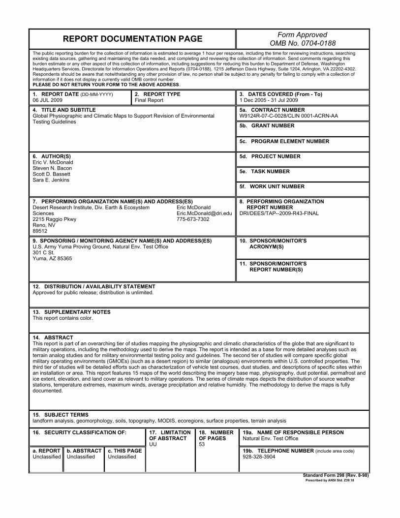
14. ABSTRACTThis report is part of an overarching tier of studies mapping the physiographic and climatic characteristics of the globe that are significant tomilitary operations, including the methodology used to derive the maps. The report is intended as a base for more detailed analyses such asterrain analog studies and for military environmental testing policy and guidelines. The second tier of studies will compare specific globalmilitary operating environments (GMOEs) (such as a desert region) to similar (analogous) environments within U.S. controlled properties. Thethird tier of studies will be detailed efforts such as characterization of vehicle test courses, dust studies, and descriptions of specific sites withinan installation or area. This report features 15 maps of the world describing the imagery base map, physiography, dust potential, permafrost andice extent, elevation, and land cover as relevant to military operations. The series of climate maps depicts the distribution of source weatherstations, temperature extremes, maximum winds, average precipitation and relative humidity. The methodology to derive the maps is fullydocumented.
15. SUBJECT TERMSlandform analysis, geomorphology, soils, topography, MODIS, ecoregions, surface properties, terrain analysis
Standard Form 298 (Rev. 8-98)Prescribed by ANSI Std. Z39.18
16. SECURITY CLASSIFICATION OF: 17. LIMITATIONOF ABSTRACTUU
18. NUMBEROF PAGES53
19a. NAME OF RESPONSIBLE PERSONNatural Env. Test Office
a. REPORTUnclassified
b. ABSTRACTUnclassified
c. THIS PAGEUnclassified
19b. TELEPHONE NUMBER (include area code)928-328-3904
Global Physiographic and Climatic Maps to Support Revision of Environmental Testing Guidelines _____________________ Eric V. McDonald Steven N. Bacon Scott D. Bassett Sara E. Jenkins _____________________ FINAL REPORT DRI/DEES/TAP--2009-R43-FINAL July 6, 2009 _____________________
Prepared by Division of Earth & Ecosystem Sciences Desert Research Institute, Nevada System of Higher Education Prepared for U.S. Army Yuma Proving Ground, Natural Environments Test Office Under contract W9124R-07-C-0028/CLIN 0001-ACRN-AA
Global Physiographic and Climatic Maps to Support Revision of Environmental Testing Guidelines
EXECUTIVE SUMMARY Introduction
The Army must provide equipment to the Warfighter that will ensure mission success
under any conditions, wherever U.S. forces may be deployed worldwide. This requires
that the materiel RDTE (Research, Development, Test and Evaluation) community has an
in-depth understanding of potential Global Military Operational Environments (GMOE)
including climate and terrain, plus the potential effects of these environmental factors on
equipment performance.
Current applicable DOD guidelines for consideration of environmental effects on
equipment performance do not provide adequate descriptive information. The primary
focus in the post-WWII decades has been on the humid-temperate regions of Europe.
Non-temperate regions were considered extreme and were described primarily by
simplified climatic factors such as max/min temperatures and daily temperature or
temperature-humidity cycles. This approach discounts the effects of seasonality,
precipitation patterns, vegetation, and possibly most importantly for ground operations,
the terrain.
This study was sponsored by the Natural Environments Test Office (NETO) of the U.S.
Army Yuma Proving Ground (YPG), Arizona. YPG is a subordinate activity of the U.S.
Army Developmental Test Command (DTC), a major component of the U.S. Army Test
and Evaluation Command (ATEC).
The effort was conducted by the Desert Research Institute as part of the overall initiative
of updating applicable Department of Army guidelines for consideration of
environmental effects during RDTE of materiel. The primary application is the revision
of Army Regulation (AR) 70-38 Research, Development, Test, and Evaluation of
Materiel for Extreme Climatic Conditions. The proposed revision of AR 70-38 describes
and defines strategic level Global Military Operational Environments (GMOE),
incorporating the concept of Bailey’s (1998) “ecoregions” classification scheme as an
organizing principle.
Final Report – July 6, 2009 A
Global Physiographic and Climatic Maps to Support Revision of Environmental Testing Guidelines
Data sources for these maps include various remote sensing datasets, readily available
online terrain and surface characteristic databases, previously published map products, as
well as original map data products generated by the Desert Research Institute. The map
series includes the following products, with brief explanations of methodology and
terminology incorporated into the production of each:
1. Global Physiographic Map
2. Global Dust Potential Map
3. Global Permafrost and Ground Ice Extent Map
4. Global Elevation Map
5. Global Land Cover Map
6. Global Climatic Maps (set of 8)
It should be noted that the suite of maps was produced at global, strategic scales for the
purpose of a general overview of the types and spatial distribution of potential
environmental and climatic factors likely to be encountered during military operations.
As a result the maps are not intended for use in detailed or site-specific hazards analyses.
Future work can expand the current methodologies to characterize specific areas or
hazards of military interest at more detailed and tactical scales (e.g., McDonald et al.,
2009).
Acknowledgements
The authors greatly acknowledge the helpful comments, suggestions, and contributions
by Graham Stullenbarger, Linda Spears, Wayne Lucas, John Hawk, and Valerie Morrill
of YPG-NETO. We also appreciate the comments and suggestions made during a peer-
review meeting of the map products by Russell Harmon of ARO, Charles Ryerson of
ERDC-CRREL-NH, and William Doe III of the Institute for Environmental Studies,
Western Illinois University. This work was funded through the U.S. Army Yuma Proving
Ground, Natural Environments Test Office under Contract W9124R-07-C-0028/CLIN
0001-ACRN-AA.
Final Report – July 6, 2009 B
Global Physiographic and Climatic Maps to Support Revision of Environmental Testing Guidelines
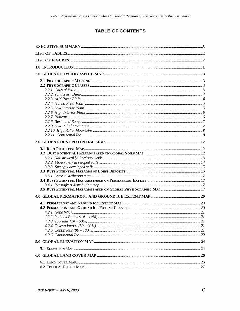
TABLE OF CONTENTS EXECUTIVE SUMMARY ..........................................................................................................................A LIST OF TABLES........................................................................................................................................E LIST OF FIGURES...................................................................................................................................... F 1.0 INTRODUCTION ................................................................................................................................. 1 2.0 GLOBAL PHYSIOGRAPHIC MAP................................................................................................... 3
2.1 PHYSIOGRAPHIC MAPPING ................................................................................................................ 3 2.2 PHYSIOGRAPHIC CLASSES ................................................................................................................. 3
2.2.1 Coastal Plain .............................................................................................................................. 3 2.2.2 Sand Sea / Dune .......................................................................................................................... 4 2.2.3 Arid River Plain .......................................................................................................................... 4 2.2.4 Humid River Plain ...................................................................................................................... 5 2.2.5 Low Interior Plain....................................................................................................................... 5 2.2.6 High Interior Plain ..................................................................................................................... 6 2.2.7 Plateau ........................................................................................................................................ 6 2.2.8 Basin and Range ......................................................................................................................... 7 2.2.9 Low Relief Mountains ................................................................................................................. 7 2.2.10 High Relief Mountains .............................................................................................................. 8 2.2.11 Continental Ice.......................................................................................................................... 8
3.0 GLOBAL DUST POTENTIAL MAP................................................................................................ 12 3.1 DUST POTENTIAL MAP..................................................................................................................... 12 3.2 DUST POTENTIAL HAZARDS BASED ON GLOBAL SOILS MAP ........................................................ 12
3.2.1 Non or weakly developed soils.................................................................................................. 13 3.2.2 Moderately developed soils ...................................................................................................... 14 3.2.3 Strongly developed soils ........................................................................................................... 15
3.3 DUST POTENTIAL HAZARDS OF LOESS DEPOSITS........................................................................... 16 3.3.1 Loess distribution map.............................................................................................................. 17
3.4 DUST POTENTIAL HAZARDS BASED ON PERMAFROST EXTENT...................................................... 17 3.4.1 Permafrost distribution map ..................................................................................................... 17
3.5 DUST POTENTIAL HAZARDS BASED ON GLOBAL PHYSIOGRAPHIC MAP ....................................... 17 4.0 GLOBAL PERMAFROST AND GROUND ICE EXTENT MAP.................................................. 20
4.1 PERMAFROST AND GROUND ICE EXTENT MAP............................................................................... 20 4.2 PERMAFROST AND GROUND ICE EXTENT CLASSES ........................................................................ 20
4.2.1 None (0%) ................................................................................................................................. 21 4.2.2 Isolated Patches (0 – 10%) ....................................................................................................... 21 4.2.3 Sporadic (10 – 50%) ................................................................................................................. 21 4.2.4 Discontinuous (50 – 90%)......................................................................................................... 21 4.2.5 Continuous (90 – 100%) ........................................................................................................... 21 4.2.6 Continental Ice.......................................................................................................................... 22
5.0 GLOBAL ELEVATION MAP........................................................................................................... 24 5.1 ELEVATION MAP................................................................................................................................ 24
6.0 GLOBAL LAND COVER MAP ........................................................................................................ 26 6.1 LAND COVER MAP............................................................................................................................. 26 6.2 TROPICAL FOREST MAP ..................................................................................................................... 27
Final Report – July 6, 2009 C
Global Physiographic and Climatic Maps to Support Revision of Environmental Testing Guidelines
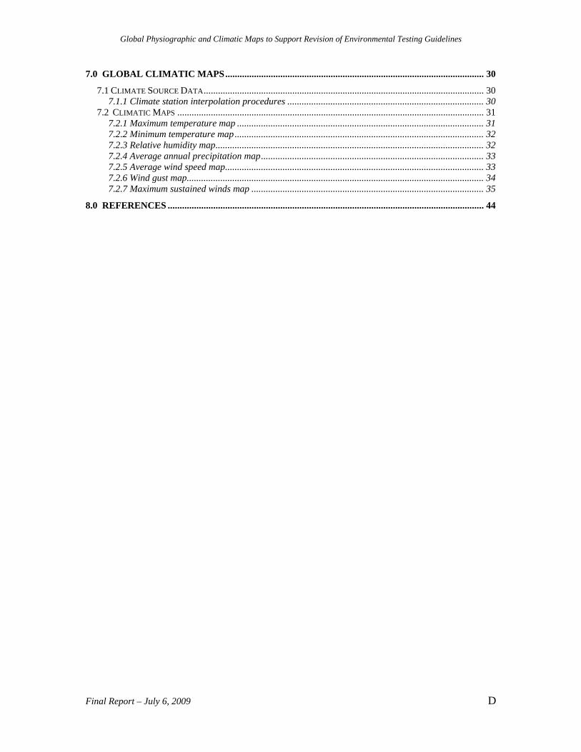
7.0 GLOBAL CLIMATIC MAPS............................................................................................................ 30
7.1 CLIMATE SOURCE DATA..................................................................................................................... 30 7.1.1 Climate station interpolation procedures .................................................................................. 30
7.2 CLIMATIC MAPS ................................................................................................................................ 31 7.2.1 Maximum temperature map ....................................................................................................... 31 7.2.2 Minimum temperature map........................................................................................................ 32 7.2.3 Relative humidity map................................................................................................................ 32 7.2.4 Average annual precipitation map............................................................................................. 33 7.2.5 Average wind speed map............................................................................................................ 33 7.2.6 Wind gust map............................................................................................................................ 34 7.2.7 Maximum sustained winds map ................................................................................................. 35
8.0 REFERENCES .................................................................................................................................... 44
Final Report – July 6, 2009 D
Global Physiographic and Climatic Maps to Support Revision of Environmental Testing Guidelines
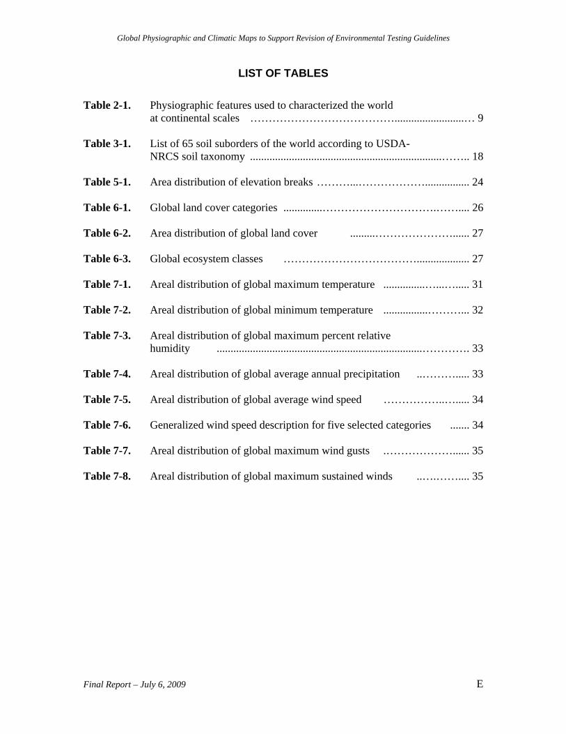
LIST OF TABLES Table 2-1. Physiographic features used to characterized the world at continental scales ………………………………….........................… 9 Table 3-1. List of 65 soil suborders of the world according to USDA- NRCS soil taxonomy .....................................................................…….. 18 Table 5-1. Area distribution of elevation breaks ………...………………................ 24 Table 6-1. Global land cover categories ..............………………………….…….... 26 Table 6-2. Area distribution of global land cover .........…………………...... 27 Table 6-3. Global ecosystem classes ………………………………................... 27 Table 7-1. Areal distribution of global maximum temperature ...............…...…..... 31 Table 7-2. Areal distribution of global minimum temperature ................………... 32 Table 7-3. Areal distribution of global maximum percent relative humidity ..........................................................................…………. 33 Table 7-4. Areal distribution of global average annual precipitation ..………..... 33 Table 7-5. Areal distribution of global average wind speed ……………..…..... 34 Table 7-6. Generalized wind speed description for five selected categories ....... 34 Table 7-7. Areal distribution of global maximum wind gusts .………………...... 35 Table 7-8. Areal distribution of global maximum sustained winds ..….…….... 35
Final Report – July 6, 2009 E
Global Physiographic and Climatic Maps to Support Revision of Environmental Testing Guidelines
LIST OF FIGURES
Figure 2-1. MODIS digital imagery for physiographic terrain identification ..…................................................……………………..... 10 Figure 2-2. Global physiographic map ..…...….………………………………..... 11 Figure 3-1. Global dust potential map ………………..………………………..... 19 Figure 4-1. Global permafrost extent map ..........................................……………..... 23 Figure 5-1. Global elevation map ..………………………………………................. 25 Figure 6-1. Global land cover map ..………………………………………..... 28 Figure 6-2. Global tropical forest map …………..……………………………..... 29 Figure 7-1. Global distribution of weather stations ………..………………..... 36 Figure 7-2. Global maximum temperature map .......…………..………………….. 37 Figure 7-3. Global minimum temperature map ………………………………....... 38 Figure 7-4. Global relative humidity map ..………………………………................. 39 Figure 7-5. Global average annual precipitation map ..………………………..... 40 Figure 7-6. Global average wind speed map ..………………………………..... 41 Figure 7-7. Global maximum wind gusts map ..………………………................. 42 Figure 7-8. Global maximum sustained wind speed map ..………………………..... 43
Final Report – July 6, 2009 F
Global Physiographic and Climatic Maps to Support Revision of Environmental Testing Guidelines
1.0 INTRODUCTION
The military operating environments and hazardous factors facing the United
States Department of Defense personnel and materiel are varied, and can include what are
generally considered climatic extremes. As such, it is essential to identify the potential
natural factors inherent in these extreme environments that may directly impact military
operations. To develop equipment that ensures mission success under any environmental
conditions, extreme or not, the Army’s Research Development, Test and Evaluation
(RDTE) community must apply this understanding of these environmental hazards and
where they are located globally throughout the acquisition process.
The maps presented in this report provide a global overview of the worldwide
military operating environments which reveal areas of the world that have analogous
environmental features of terrain, climate, and vegetation. This is the first level of effort
to understand and compare areas of interest to sites that are within the U.S. or are
otherwise accessible to the RDTE community. Continuing studies will address more
detailed levels that bring this understanding to an in depth characterization of specific
areas and their analog test sites.
This report provides documentation of methods, statistical approaches, and
sources of information used to generate 15 global maps depicting environmental
conditions with the potential to influence military activities and equipment operation. The
mapping was performed under Contract W9124R-07-C-0028/CLIN 0001-ACRN-AA to
support the efforts of U.S. Army Yuma Proving Ground Natural Environments Test
Office (TEDT-YP-NE) and to update current environmental guidelines such as Army
Regulation (AR) 70-38: Research, Development, Test, and Evaluation of Materiel for
Extreme Climatic Conditions.
The proposed revision of environmental guidelines describes and defines Global
Military Operational Environments (GMOE) at a strategic level, incorporating Bailey’s
(1998) “ecoregions” classification scheme as an organizing principle. The additional
Final Report – July 6, 2009 1
Global Physiographic and Climatic Maps to Support Revision of Environmental Testing Guidelines
global maps presented in this report will be used to both directly supplement the Bailey’s
ecoregions maps and will be used to instruct and guide revision efforts of other
documents through presentation and summary of a wide range of global environmental
conditions. In other words, the attached maps provide multiple views of key global
environmental conditions that will enhance identification of the type and the global
distribution of environmental conditions most likely to impact military operations.
Use of these preliminary, small-scale maps should be restricted to situations
where a generalized understanding of physiographic features and surface characteristics
is useful. This suite of maps is not recommended as a data source for situations in which
a highly detailed, large-scale interpretation of surface characteristics is necessary, or for
the establishment of maximum or minimum values of factors such as temperature. Future
work, if requested, can expand the current methodologies employed in this report to
devise products suitable for larger, tactical scale mission planning (e.g., McDonald et al.,
2009).
Final Report – July 6, 2009 2
Global Physiographic and Climatic Maps to Support Revision of Environmental Testing Guidelines
2.0 GLOBAL PHYSIOGRAPHIC MAP 2.1 Physiographic Mapping
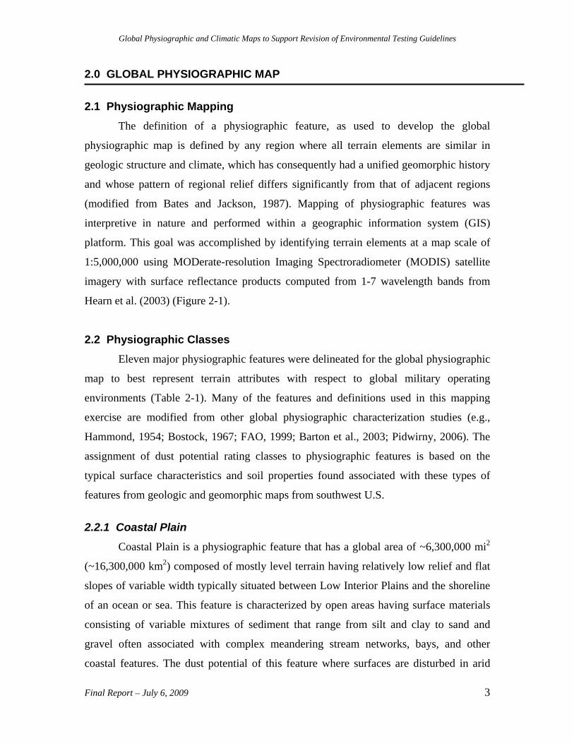
The definition of a physiographic feature, as used to develop the global
physiographic map is defined by any region where all terrain elements are similar in
geologic structure and climate, which has consequently had a unified geomorphic history
and whose pattern of regional relief differs significantly from that of adjacent regions
(modified from Bates and Jackson, 1987). Mapping of physiographic features was
interpretive in nature and performed within a geographic information system (GIS)
platform. This goal was accomplished by identifying terrain elements at a map scale of
1:5,000,000 using MODerate-resolution Imaging Spectroradiometer (MODIS) satellite
imagery with surface reflectance products computed from 1-7 wavelength bands from
Hearn et al. (2003) (Figure 2-1).
2.2 Physiographic Classes
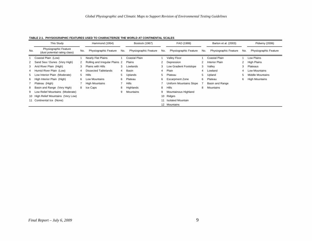
Eleven major physiographic features were delineated for the global physiographic
map to best represent terrain attributes with respect to global military operating
environments (Table 2-1). Many of the features and definitions used in this mapping
exercise are modified from other global physiographic characterization studies (e.g.,
Hammond, 1954; Bostock, 1967; FAO, 1999; Barton et al., 2003; Pidwirny, 2006). The
assignment of dust potential rating classes to physiographic features is based on the
typical surface characteristics and soil properties found associated with these types of
features from geologic and geomorphic maps from southwest U.S.
2.2.1 Coastal Plain Coastal Plain is a physiographic feature that has a global area of ~6,300,000 mi2
(~16,300,000 km2) composed of mostly level terrain having relatively low relief and flat
slopes of variable width typically situated between Low Interior Plains and the shoreline
of an ocean or sea. This feature is characterized by open areas having surface materials
consisting of variable mixtures of sediment that range from silt and clay to sand and
gravel often associated with complex meandering stream networks, bays, and other
coastal features. The dust potential of this feature where surfaces are disturbed in arid
Final Report – July 6, 2009 3
Global Physiographic and Climatic Maps to Support Revision of Environmental Testing Guidelines
environments is generally Low. The elevation of this feature typically ranges from 0 to
500 ft (0 to 150 m). The most common elevation within the feature is sea level extending
up to 3 ft (up to 1 m) (Figure 2-2).
2.2.2 Sand Sea / Dune Sand Sea / Dune is a physiographic feature with a global area of ~4,600,000 mi2
(~12,000,000 km2), consisting mostly of level and hilly terrain in the form of mounds,
ridges, or hills of wind-blown sediment, either bare or covered with vegetation. Surface
materials are composed mostly of loose and well-sorted sand and minor silt. Sand Sea /
Dune fields, also known as ergs, are vast regions where sand accumulates into systems of
hills or mega-dunes that exceed 300 ft (100 m) in height or as relatively flat sandy plains,
which are both found in the Sahara Deserts of North Africa and the Arabian Peninsula. In
areas where the source of sandy sediment is relatively low, linear and relatively narrow
(barchan) shaped dunes are often underlain by hard and competent bedrock, gravelly
desert pavement (regs), or silty playa/sabkha surfaces, which are exposed between the
ridges of linear dunes. The dust potential of this feature in semi-arid to arid environments
can be Very High. The elevation of this feature ranges from 0 to 3200 ft (0 to 1000 m),
but mostly from 0 to 1600 ft (0 to 600 m). The most common elevation within the feature
is 1000 ft (300 m) (Figure 2-2).
2.2.3 Arid River Plain
Arid River Plain is a physiographic feature that has a total area of ~1,000,000 mi2
(~2,600,000 km2) composed of flat to hilly terrain. The area of an Arid River Plain is
drained by a network of poorly to moderately developed anastomosing and braided rivers
and associated tributaries across mostly low to moderate slopes. Surface materials consist
of variable mixtures of sediment that range from silt and clay to sand and gravel. Arid
River Plains often occur within continental settings and are internally drained such as the
Caspian Sea region of southwest Asia or drain to the ocean, such as the Nile River in
Egypt and the Tigris and Euphrates Rivers in Iraq. Regions characterized as Arid River
Plain are typically located within semi-arid to arid environments and receive relatively
less precipitation than Humid River Plains. The dust potential of disturbed surfaces in
Final Report – July 6, 2009 4
Global Physiographic and Climatic Maps to Support Revision of Environmental Testing Guidelines
arid environments is typically High. The elevation of this feature ranges from 0 to 1000 ft
(0 to 300 m), but mostly from 300 to 650 ft (100 to 200 m). The most common elevation
within the feature is ~500 ft (~150 m) (Figure 2-2).
2.2.4 Humid River Plain Humid River Plain is a physiographic feature that has a global area of ~3,400,000
mi2 (~8,900,000 km2) that commonly includes the area drained by numerous well-
developed river systems and associated dense network of tributaries. Slopes within the
feature range from low near Coastal Plains to moderate associated with dissected rolling
hills adjacent to Low Interior Plains and Plateaus. Surface materials consist of variable
mixtures of sediment that range from silt and clay to sand and gravel that is often mantled
by a thick organic silty and clayey soil. Regions characterized as Humid River Plain
typically occur within temperate to tropical environments having high precipitation and
boarded by High and Low Relief Mountains or Interior Plains and Plateaus, such as the
Amazon River Basin in South America and the Congo River Basin in Africa. The dust
potential of disturbed surfaces under dry conditions within this physiographic feature is
generally Low. The elevation of this feature ranges from 0 to 1500 ft (0 to 450 m), but
mostly from 300 to 1000 ft (100 to 300 m). The most common elevation within the
feature is ~300 ft (~100 m) (Figure 2-2).
2.2.5 Low Interior Plain Low Interior Plain is a broad upland physiographic feature that has a total area of
~12,300,000 mi2 (~31,800,000 km2) consisting mostly of level terrain. Low Interior
Plains are often bounded by Coastal Plains, High Interior Plains or Low and High Relief
Mountains. This feature has relatively low relief and mostly flat to gentle slopes that are
often associated with meandering and straight stream networks, as well as steeper slopes
that are commonly associated with major stream valleys. Surface materials consist of
variable mixtures of sediment that range from clay and silt to sand and gravel. A
relatively thick silt cap (loess sheet) often covers Low Interior Plain surfaces within semi-
arid to arid environments, such as the central interior of Australia; therefore the dust
potential of disturbed surfaces is typically Moderate. The elevation of low interior plains
Final Report – July 6, 2009 5
Global Physiographic and Climatic Maps to Support Revision of Environmental Testing Guidelines
typically ranges from 500 to 2000 ft (150 to 600 m). The most common elevation within
the feature is ~1000 ft (~300 m) (Figure 2-2).
2.2.6 High Interior Plain High Interior Plain is a broad upland physiographic feature that has a total area of
~6,500,000 mi2 (~16,700,000 km2) consisting mostly of level and rolling terrain. This
feature exhibits low to moderate slopes that often have straight stream networks having
drainage divides with steep slopes which are commonly associated with major stream
valleys. Surface materials consist of variable mixtures of sediment that range from clay
and silt to sand and gravel. A relatively thick silt cap (loess sheet) is often present within
temperate to arid environments, such as the central interior of North America and
Eurasia, therefore the dust potential of disturbed surfaces is mostly High. The elevation
of High Interior Plains typically ranges from 1000 to 5000 ft (300 to 1500 m). The most
common elevation within the feature is ~1600 ft (~500 m) (Figure 2-2).
2.2.7 Plateau Plateau is a physiographic feature that has a total area of ~4,500,000 mi2
(~11,500,000 km2) consisting of broad and rugged mountainous terrain. A plateau is an
extensive region of land considerably elevated more than 500 to 1000 ft (150 to 300 m)
above adjacent regions or above sea level and is commonly limited on at least one side by
an abrupt descent. It also has a nearly flat or smooth surface, but is often dissected by
deep valleys and surmounted by Low or High Relief Mountains, as well as has a large
part of its total surface at or near the summit level. A Plateau is usually higher in
elevation and exhibits more noticeable relief than a High Interior Plain. Surface materials
consist mostly of loose sandy, gravelly, and cobbly sediment underlain by competent and
resistant bedrock. A network of deeply incised drainages or valleys are often present
having slopes that range from steep to precipitous, such as the Colorado Plateau in the
southwest United States. A relatively thick silt cap (loess sheet) is often present within
semi-arid to arid environments, such as the central interior of North America, Africa, and
Eurasia, therefore the dust potential of disturbed surfaces typically is High. The elevation
of Plateau features typically range from 1000 to 7200 ft (300 to 2200 m). The most
Final Report – July 6, 2009 6
Global Physiographic and Climatic Maps to Support Revision of Environmental Testing Guidelines
common elevation within the feature is ~3600 ft (~1100 m), but can reach elevations as
high as ~16,400 ft (~5000 m) adjacent to the Himalayan Mountains of central Asia
(Figure 2-2).
2.2.8 Basin and Range Basin and Range is a physiographic feature that has a total area of ~1,100,000 mi2
(~3,000,000 km2) consisting of broken, flat and rugged mountainous terrain. The Basin
and Range is characterized as a region that exhibits a series of relatively parallel and
longitudinal, asymmetric Low and High Relief Mountains separated by broad and linear
intervening basins or Low Interior Plains. Surface materials of the Low and High Relief
Mountains consist mostly of loose sandy, gravelly, and cobbly sediment underlain by
competent and resistant bedrock, whereas the intervening basins materials range from
clay and silt to sand and gravel. Many basins contain lakes, playas, and alluvial plains
providing a source of primary silt, as well as secondary silt that influences the
development of a regional silt cap (loess sheet) of variable thickness. As result, the dust
potential of disturbed surfaces is generally Very High within semi-arid to arid
environments, such as the Basin and Range Province in the western United States. The
elevation of the Basin and Range is between 1000 to 16,400 ft (300 to 5000 m). The most
common elevation of both the basins and ranges within the feature is between ~3600 and
7200 ft (~1100 and 2200 m), but the elevation of the mountainous ranges commonly
occur between ~9,800 and 13,100 ft (~3000 and 4000 m) (Figure 2-2).
2.2.9 Low Relief Mountains Low Relief Mountains is a physiographic feature that has a total area of
~4,000,000 mi2 (~10,400,000 km2) consisting of hilly to rugged mountainous terrain that
often is traversed by well-developed river valleys. Low Relief Mountains are
characterized as a region of relatively low to moderate relief that has slopes that range
from moderate to very steep, such as the Appalachian Mountains in eastern United States.
Surface materials consist mostly of loose sandy, gravelly, and cobbly sediment underlain
by competent and resistant bedrock, whereas within narrow river valleys, surface
materials range from clay and silt to sand and gravel. The dust potential of disturbed
Final Report – July 6, 2009 7
Global Physiographic and Climatic Maps to Support Revision of Environmental Testing Guidelines
Final Report – July 6, 2009 8
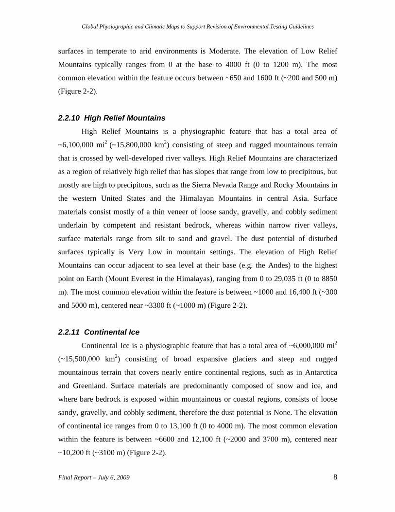
surfaces in temperate to arid environments is Moderate. The elevation of Low Relief
Mountains typically ranges from 0 at the base to 4000 ft (0 to 1200 m). The most
common elevation within the feature occurs between ~650 and 1600 ft (~200 and 500 m)
(Figure 2-2).
2.2.10 High Relief Mountains High Relief Mountains is a physiographic feature that has a total area of
~6,100,000 mi2 (~15,800,000 km2) consisting of steep and rugged mountainous terrain
that is crossed by well-developed river valleys. High Relief Mountains are characterized
as a region of relatively high relief that has slopes that range from low to precipitous, but
mostly are high to precipitous, such as the Sierra Nevada Range and Rocky Mountains in
the western United States and the Himalayan Mountains in central Asia. Surface
materials consist mostly of a thin veneer of loose sandy, gravelly, and cobbly sediment
underlain by competent and resistant bedrock, whereas within narrow river valleys,
surface materials range from silt to sand and gravel. The dust potential of disturbed
surfaces typically is Very Low in mountain settings. The elevation of High Relief
Mountains can occur adjacent to sea level at their base (e.g. the Andes) to the highest
point on Earth (Mount Everest in the Himalayas), ranging from 0 to 29,035 ft (0 to 8850
m). The most common elevation within the feature is between ~1000 and 16,400 ft (~300
and 5000 m), centered near ~3300 ft (~1000 m) (Figure 2-2).
2.2.11 Continental Ice Continental Ice is a physiographic feature that has a total area of ~6,000,000 mi2
(~15,500,000 km2) consisting of broad expansive glaciers and steep and rugged
mountainous terrain that covers nearly entire continental regions, such as in Antarctica
and Greenland. Surface materials are predominantly composed of snow and ice, and
where bare bedrock is exposed within mountainous or coastal regions, consists of loose
sandy, gravelly, and cobbly sediment, therefore the dust potential is None. The elevation
of continental ice ranges from 0 to 13,100 ft (0 to 4000 m). The most common elevation
within the feature is between ~6600 and 12,100 ft (~2000 and 3700 m), centered near
~10,200 ft (~3100 m) (Figure 2-2).
Global Physiographic and Climatic Maps to Support Revision of Environmental Testing Guidelines
TABLE 2-1. PHYSIOGRAPHIC FEATURES USED TO CHARACTERIZE THE WORLD AT CONTINENTAL SCALES
1 1 1 1 1 12 2 2 2 2 23 3 3 3 3 34 4 4 4 4 45 5 5 5 5 56 6 6 6 6 67 7 7 7 78 8 8 8 89 9 910 1011 11
12
High Mountains
High PlainsPlateausLow MountainsMiddle Mountains
Pidwrny (2006)
No. Physiographic Feature
Low Plains
Mountainous HighlandRidgesIsolated MountainMountains
No. Physiographic Feature
Valley FloorDepression
FAO (1999)
Low Gradient FootslopePlainPlateauEscarpment ZoneUniform Mountains SlopeHills
No.
Barton et al. (2003)
Physiographic Feature
Coastal PlainInterior PlainValleyLowlandUplandPlateauBasin and RangeMountains
PlateauHillsHighlandsMountains
Bostock (1967)
No. Physiographic Feature
Coastal PlainPlains LowlandsBasinUplands
Low MountainsHigh MountainsIce Caps
High Relief Mountains (Very Low)Continental Ice (None)
No.
Hammond (1954)
Physiographic Feature
Nearly Flat PlainsRolling and Irregular PlainsPlains with HillsDissected TablelandsHills
High Interior Plain (High)Plateau (High)Basin and Range (Very High)Low Relief Mountains (Moderate)
Sand Sea / Dunes (Very High)Arid River Plain (High)Humid River Plain (Low)Low Interior Plain (Moderate)
This Study
Physiographic Feature (dust potential rating class)No.
Coastal Plain (Low)
Final Report – July 6, 2009 9
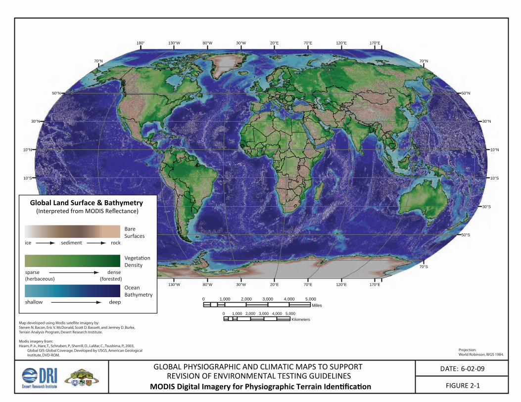
FIGURE 2-1
DATE: 6-02-09GLOBAL PHYSIOGRAPHIC AND CLIMATIC MAPS TO SUPPORTREVISION OF ENVIRONMENTAL TESTING GUIDELINES
MODIS Digital Imagery for Physiographic Terrain Identification
170°E
170°E
120°E
120°E
70°E
70°E
20°E
20°E
30°W
30°W
80°W
80°W
130°W
130°W
180°
180°
50°N 50°N
30°N 30°N
10°N 10°N
10°S 10°S
30°S 30°S
50°S
70°N 70°N
50°S
70°S 70°S
Map developed using Modis satellite imagery by:Steven N. Bacon, Eric V. McDonald, Scott D. Bassett, and Jermey D. Burke,Terrain Analysis Program, Desert Research Institute.
Modis imagery from:Hearn, P. Jr., Hare, T., Schruben, P., Sherrill, D., LaMar, C., Tsushima, P., 2003, Global GIS: Global Coverage, Developed by USGS, American Geological Institute, DVD-ROM.
Projection: World Robinson, WGS 1984.
0 1,000 2,000 3,000 4,000 5,000Miles
0 1,000 2,000 3,000 4,000 5,000Kilometers
Ocean Bathymetry
shallow deep
BareSurfaces
ice sediment rock
Vegetation Density
sparse dense(herbaceous) (forested)
Global Land Surface & Bathymetry (Interpreted from MODIS Reflectance)
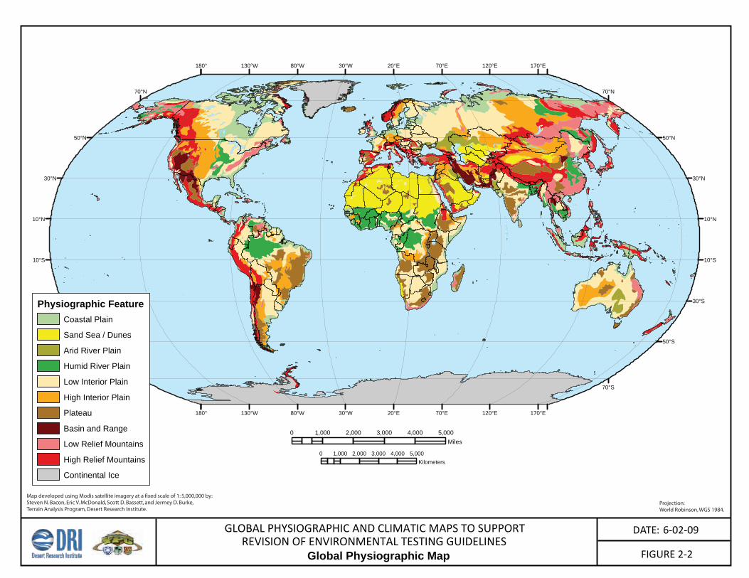
REVISION OF ENVIRONMENTAL TESTING GUIDELINESFIGURE 2-2
DATE: 6-02-09GLOBAL PHYSIOGRAPHIC AND CLIMATIC MAPS TO SUPPORT
Global Physiographic Map
170°E
170°E
120°E
120°E
70°E
70°E
20°E
20°E
30°W
30°W
80°W
80°W
130°W
130°W
180°
180°
50°N 50°N
30°N 30°N
10°N 10°N
10°S 10°S
30°S 30°S
50°S
70°N 70°N
50°S
70°S 70°S
0 1,000 2,000 3,000 4,000 5,000Miles
0 1,000 2,000 3,000 4,000 5,000Kilometers
Map developed using Modis satellite imagery at a fixed scale of 1: 5,000,000 by:Steven N. Bacon, Eric V. McDonald, Scott D. Bassett, and Jermey D. Burke,Terrain Analysis Program, Desert Research Institute.
Projection: World Robinson, WGS 1984.
Physiographic FeatureCoastal Plain
Sand Sea / Dunes
Arid River Plain
Humid River Plain
Low Interior Plain
High Interior Plain
Plateau
Basin and Range
Low Relief Mountains
High Relief Mountains
Continental Ice
Global Physiographic and Climatic Maps to Support Revision of Environmental Testing Guidelines
3.0 GLOBAL DUST POTENTIAL MAP
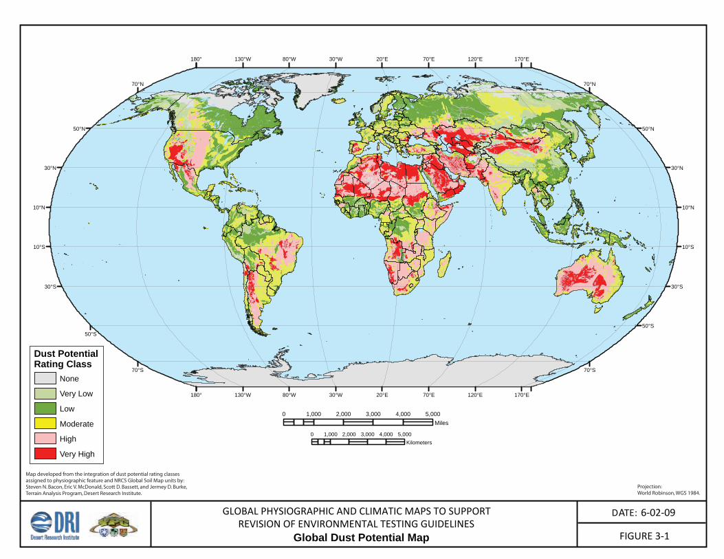
3.1 Dust Potential Map The global dust potential map is based on the integration of (1) the global soil map of
the United State Department of Agriculture, Natural Resources Conservation Service
(USDA-NRCS) at the suborder level according to the soil taxonomic system (Soil Survey
Staff, 1999); (2) the global distribution of mapped loess deposits; (3) the Circum-Arctic
permafrost and ground ice map of Brown et al. (1998); and (4) the global physiographic map
and associated dust potential hazard classes presented in this report (see Section 2.0; Table 2-
1). A six-fold hazard class system (None, Very Low, Low, Moderate, High, and Very High)
was developed to categorize the disturbed (anthropogenic) dust potential for significant
amounts of dust emission on a global scale during dry environmental conditions. The dust
potential was quantified by assigning a numerical value to each hazard class, and normalizing
the summed hazard ratings for each of the aforementioned four dust potential map products
to match the original six-fold rating class scheme (Figure 3-1).
3.2 Dust Potential Hazards based on Global Soils Map The USDA-NRCS global soils map used for dust potential hazards is a derivative
product that represents a translation from FAO to USDA soil taxonomy (Soil Survey Staff,
1999). It is generated from the overlay of the NRCS soil climate map on FAO soil
classification maps (e.g. FAO-UNESCO-ICRIS 1988; 1990; 1998), which at present, are the
only global soils maps available. For background, soil is considered to be a 3-dimensional
body with properties that reflect the impact of (1) climate, (2) vegetation and fauna, (3)
topography, (4) parent material, and (5) length of time (e.g., Nachtergaele et al., 2000). The
FAO soil classification system is defined in terms of measurable and observable properties of
the soil itself having diagnostic horizons (FAO-UNESCO-ICRIS, 1988). The USDA Soil
Taxonomy (Soil Survey Staff, 1999) also classifies soil orders according to the presence or
absence of diagnostic soil horizons, as a reflection of the degree of soil development.
Therefore, each of the 106 individual global FAO soil units can be correlated by soil
development, material, and major geographical zone to 65 soil suborders (e.g. order Aridisol
“arid soil”, suborder Argid “arid clay-rich soil” within the USDA soil taxonomy system).
Each USDA suborder was then assigned a specific dust hazard class based on typical
Final Report – July 6, 2009 12
Global Physiographic and Climatic Maps to Support Revision of Environmental Testing Guidelines
attributes that cause dust emission when the upper 1.0 foot (0.3 meter) of the soil profile is
disturbed under dry environmental conditions (Table 3-1; Figure 3-1).
The criteria used to assign specific hazard classes to soil units include the following:
(1) geographical zone; (2) silt, clay, and sand particle-size fraction; (3) salt content; and (4)
approximate depth to groundwater. The following sub-sections provide a brief description of
each major soil order. Individual soil orders and suborders are described in more detail in the
USDA publication Soil Taxonomy (Soil Survey Staff, 1999).
3.2.1 Non or weakly developed soils
Rock: outcrops of bare rock with no soil development were designated to have a dust
potential hazard of None (Table 3-1).
Entisols: are mineral soils formed in recent deposits with minimal to no genetic horizon
development. The unifying feature of this diverse and widely distributed soil order is their
lack of soil formation beyond the earliest stages of development; they are either very young
deposits, or have not responded to soil-forming influences. Dust potential varies within this
order as a function of typical soil water content and its seasonal distribution (Table 3-1).
Andisols: are young, poorly weathered soils that are commonly formed on volcanic ash and
cinders located proximal to – and downwind of – volcanic centers. They are defined by a set
of andic properties that include a high percentage of volcanic glass and/or poorly crystallized
or amorphous iron and aluminum minerals, often with thick organic horizons, and a high
water holding capacity. Except for Aquands (defined by near-surface water), this order
exhibits Moderate to Very High variable dust potential hazards depending on amount and
seasonality of the soil moisture regime (Table 3-1).
Inceptisols: are soils in which incipient profile development is evident, though ‘mature’ soil
properties are not yet distinguishable. Generally formed in young deposits, they are most
common to mountainous areas, particularly in the tropics. Similar to Entisols, this soil order
Final Report – July 6, 2009 13
Global Physiographic and Climatic Maps to Support Revision of Environmental Testing Guidelines
is widely distributed and diverse, but displays somewhat greater profile development.
Potential dust hazards vary with regional climate, and are generally Low. Ustepts and
Xerepts exhibit a High dust potential due to limited soil moisture content (Table 3-1),
particularly during the dry season.
Gelisols: are young soils that form slowly under cold and/or frozen conditions for much of
the year. Permafrost beneath the soil surface is a defining characteristic of this soil suborder,
and many show evidence of cryoturbation as water expands and contracts during freeze/thaw
cycles. Because these soils are typically frozen or saturated by water for the majority of the
year, dust potential hazard is None or Very Low (Table 3-1).
Histosols: are the soils of bogs and wetlands, most common in cold climates. They exhibit
little profile development due to the anaerobic (oxygen-poor) bog or wetland condition,
which hinders decomposition of organic materials. Horizon characteristics in Histosols vary
with the type of organic material input, rather than mineral accumulation and translocation.
High water content produces a Very Low dust potential hazard for all Histosols (Table 3-1).
3.2.2 Moderately developed soils
Aridisols: constitute the most widely distributed global soil order. These soils are
characterized by their relatively low water content; by definition these soils typically cannot
exceed 90 consecutive days of soil moisture available to support vegetation growth.
Consequently, these soils often exhibit mineral accumulations at depth – that under higher
moisture regimes would be flushed from the profile – including calcium carbonate, gypsum,
soluble salts, or sodium. Some Aridisols have clay-rich subsurface horizons that may
represent a previous period of soil formation under wetter climatic conditions. These soils are
often capped with desert pavement, a one clast-thick layer of pebbles supported on an
accretionary layer of windblown silt. When pavements are removed, this fine silt is subject to
rapid wind erosion. This soil order tends to have a High to Very High dust potential hazard
(Table 3-1), a result of the brief moisture availability and/or accretionary silt cap.
Final Report – July 6, 2009 14
Global Physiographic and Climatic Maps to Support Revision of Environmental Testing Guidelines
Vertisols: have a relatively high clay content (>30%). They are identified by the swelling and
shrinking of clays within the soil profile, which occurs through consecutive wetting and
drying of calcium and magnesium-rich clays. They are characteristic of subhumid to semiarid
environments with bimodal moisture availability, but can be found in a few cold
environments as well. During dry periods, large cracks develop in the soil profile, which are
subsequently healed during wet times. Progressive cracking and swelling causes large soil
blocks to shift slightly and rub against each other, producing slick-sided, tilted surfaces
(slickensides). Dust potential hazards are highly variable for the Vertisol order. In humid or
cold climates, dust hazard potential is None to Moderate; under regimes with hot and dry
summers (e.g. Torrerts, Xererts), dust potential hazards are High to Very High (Table 3-1).
Mollisols: are organic-rich, highly fertile soils, typically with clay-rich subsurface horizons.
Most develop under grass vegetation, but Mollisols may also occur in forested regions. Dust
potential hazards are highly variable for the Mollisol order and are dependent on moisture
availability within the soils. In humid or cold climates, dust hazard potential is Very Low to
Moderate; under regimes with hot or dry summers (e.g. Xerolls, Rendolls) dust potential
hazards are High to Very High when soils are disturbed (Table 3-1).
Alfisols: form in forested environments and are more highly weathered than other moderately
developed soil orders. In the subsurface, moderate cation leaching and strong silicate clay
accumulation are diagnostic features. Dust potential hazards are extremely variable for
Alfisols and are dependent on moisture availability within the soils. In humid or cold
climates, dust hazard potential is Very Low to Moderate; under regimes with dry summers
(e.g. Xeralfs) dust potential hazards are High when soils are disturbed (Table 3-1).
3.2.3 Strongly developed soils
Ultisols: develop as a result of strong clay weathering and accumulation in the subsurface,
accompanied by available cation deficiency. These factors are typically associated with
moist, warm climates; soils form beneath a broad variety of ecosystems, from forests to
savannas to swamps. These soils, like other clay-rich soils, tend to have a Very Low to
Final Report – July 6, 2009 15
Global Physiographic and Climatic Maps to Support Revision of Environmental Testing Guidelines
Moderate dust potential when disturbed, except where associated with seasonally dry
summer moisture regimes (e.g. Xerults) (Table 3-1).
Spodosols: are acidic, sandy forest soils with low base saturation. They form under moist to
wet conditions with a broad range of temperature regimes, and are typically associated with
forest vegetation, particularly coniferous forests whose decaying needles supply necessary
acidity for soil formation. Acid leaching produces a diagnostic, white, leached horizon in the
subsurface that has been stripped of available minerals. High water content and a thick
organic cap yield a Very Low dust potential when disturbed (Table 3-1).
Oxisols: are the most highly weathered soils in the USDA-NRCS soil taxonomy system.
These form in hot climates with continual moisture availability, typically thought to occur
only beneath tropical rainforests, though some Oxisols (e.g. Torrox) occur in hot and dry
environments, likely remnants from a previously warm and wet climate. They are identified
by their relatively high, non-swelling, low-acidity clay content which lends stability and
resistance to compaction to these soils. Dust potential hazards are highly variable for Oxisols
and are dependent on moisture availability within the soils. In humid to wet environments,
dust hazard potential is Very Low to Moderate; under hot and dry regimes (e.g. Torrox) dust
potential is Very High when soils are disturbed (Table 3-1).
3.3 Dust Potential Hazards of Loess Deposits
Loess is a terrestrial deposit of eolian (wind-blown) dust composed predominately of
silt-sized particles. Most loess deposits have been altered to some degree by soil-forming
processes as deposits have accumulated through time, and their unique properties create
highly fertile agricultural soils that are some of the most productive in the world. Loess
deposits cover approximately 10% of the Earth’s land surface and are generally associated
with semi-arid to semi-humid regions, as well as downwind of desert areas. Loess deposits
are found on all continents, except for Antarctica (Busacca and Sweeney, 2005).
Final Report – July 6, 2009 16
Global Physiographic and Climatic Maps to Support Revision of Environmental Testing Guidelines
Final Report – July 6, 2009 17
3.3.1 Loess distribution map The world distribution map of major loess deposits of Busacca and Sweeney (2005)
was also incorporated into global dust potential map. Based on a high silt content and
occurrence within relatively arid regions, these deposits are classified as having a High dust
potential when disturbed during the dry season (Figure 3-1), regardless of soil taxonomy.
3.4 Dust Potential Hazards based on Permafrost Extent The Circum-Arctic permafrost and ground ice map of Brown et al. (1998) was
integrated with the USDA-NRCS soil and loess deposit maps to better define the spatial
distribution of areas that exhibit no dust potential. The subsequent Section 4.0 discusses the
permafrost extent mapping of Brown et al. (1998) in more detail.
3.4.1 Permafrost distribution map
The global distribution of continuous (90-100%) and discontinuous (50-90%) extent
of permafrost and ground ice was considered to have no dust potential (None), based on the
presence of continental ice or glaciers (surface ice) and permafrost (ground ice) throughout
the year (see Section 4.0; Figure 4-1). In areas where permafrost soils were mapped by the
USDA-NRCS (e.g. Gelisols), permafrost/ground ice coverage from the Brown et al. (1998)
map was given preference in determining dust potential.
3.5 Dust Potential Hazards based on Global Physiographic Map The assignment of dust potential rating classes to physiographic features is based on
the general surface characteristics (smooth or rough) and soil properties (particle size
distribution) of each of the eleven physiographic map features, independent of environmental
conditions. Section 2.0 discusses the global physiographic mapping and associated dust
potential rating classes in more detail.

Global Physiographic and Climatic Maps to Support Revision of Environmental Testing Guidelines
NON OR WEAK L Y DE VE L OPE D S OIL SEntisols Dust Potential Inceptisols Dust Potential Andisols Dust Potential Gelisols Dust PotentialAquents Very Low Aquepts Very Low Aquands Very Low Turbels NoneOrthents Moderate Cryepts Very Low Ustands Moderate Histels Very LowFluvents High Gelepts Very Low Vitrands Moderate Orthels Very LowPsamments Very High Anthrepts Low Cryands High
Udepts Low Xerands High Histosols Dust PotentialUstepts High Torrands Very High Fibrists Very LowXerepts High Hemists Very Low
Saprists Very Low
MODE RATE L Y DE VE L OPE D S OIL SAridisols Dust Potential Vertisols Dust Potential Mollisols Dust Potential Alfisols Dust PotentialArgids High Cryerts None Aquolls Very Low Aqualfs Very LowCryids High Aquerts Very Low Cryolls Very Low Cryalfs Very LowCalcids Very High Uderts Low Gelolls Very Low Udalfs LowCambids Very High Usterts Moderate Udolls Low Ustalfs ModerateDurids Very High Xererts High Albolls Moderate Xeralfs HighGypsids Very High Torrerts Very High Ustolls ModerateSalids Very High Rendolls High
Xerolls High
S TRONGL Y DE VE L OPE D S OIL S MIS C E L L ANEOUSUltisols Dust Potential Spodosols Dust Potential Oxisols Dust Potential Type Dust PotentialAquults Very Low Aquods Very Low Aquox Very Low Ice NoneHumults Low Cryods Very Low Perox Very Low Rock NoneUdults Low Gelods Very Low Udox Low Shifting Sand Very HighUstults Moderate Humods Very Low Ustox ModerateXerults High Orthods Very Low Torrox Very High
TABLE 3‐1. L IS T OF 65 S O IL S UBOR DE R S OF THE WOR LD AC C OR DING TO US DA‐NR C S S O IL TAXONOMY (1999) C LAS S IF IC AT ION S Y S TEM, WITH AS S IGNE D DUS T POTE NT IAL R AT ING HAZAR D C LAS S E S
Final Report – July 6, 2009 18
REVISION OF ENVIRONMENTAL TESTING GUIDELINESFIGURE 3-1
DATE: 6-02-09GLOBAL PHYSIOGRAPHIC AND CLIMATIC MAPS TO SUPPORT
Global Dust Potential Map
170°E
170°E
120°E
120°E
70°E
70°E
20°E
20°E
30°W
30°W
80°W
80°W
130°W
130°W
180°
180°
50°N 50°N
30°N 30°N
10°N 10°N
10°S 10°S
30°S 30°S
50°S
70°N 70°N
50°S
70°S 70°S
Map developed from the integration of dust potential rating classes assigned to physiographic feature and NRCS Global Soil Map units by:Steven N. Bacon, Eric V. McDonald, Scott D. Bassett, and Jermey D. Burke,Terrain Analysis Program, Desert Research Institute.
Projection: World Robinson, WGS 1984.
Dust Potential
None
Very Low
Low
Moderate
High
Very High
Rating Class
0 1,000 2,000 3,000 4,000 5,000Miles
0 1,000 2,000 3,000 4,000 5,000Kilometers
Global Physiographic and Climatic Maps to Support Revision of Environmental Testing Guidelines
4.0 GLOBAL PERMAFROST AND GROUND ICE EXTENT MAP
4.1 Permafrost and Ground Ice Extent Map Permafrost is a layer of soil, sediment or rock at varying depths below the surface in
which the temperature has remained at or below freezing continuously for at least two years.
It occurs both on land and beneath offshore arctic continental shelves, and underlies about
22% of the Earth’s surface (Permafrost subcommittee, 1998). Ground ice is mostly frozen
water which has remained well below freezing for more than two years, which also includes
alpine glaciers in mountainous regions and thick continental ice caps. The thickness of
permafrost and related features is variable at many scales and typically is governed by
overburden cover. Lowlands, highlands, and intra- and intermontane depressions are
typically characterized by thick overburden cover of greater than 15-30 ft (5-10 m), whereas
mountains and plateaus exhibit thin overburden cover less than 15-30 ft (5-10 m) and
exposed bedrock (Brown et al., 1998). The circum-arctic map of permafrost and ground ice
conditions in the northern hemisphere of Brown et al. (1998) was modified to better show the
distribution of these features at a global scale. The original mapping of Brown et al. (1998)
was developed in collaboration with the Cold Regions Research and Engineering Laboratory
(CRREL) and U.S. Geological Survey (USGS).
4.2 Permafrost and Ground Ice Extent Classes The six permafrost and ground ice classes of Brown et al. (1998) were used to best
approximate conditions of concern for military operating environments in arctic terrain
(Figure 4-1). The six classes of permafrost extent are estimated in percent area (None; 0-
10%; 10-50%; 50-90%; 90-100%; and Continental Ice). The global physiographic mapping
of high relief mountains of Section 2.0 of this report was used for regions in the southern
hemisphere that were not included on the map of Brown et al. (1998). The high relief
mountains in the southern hemisphere were assigned permafrost and ground ice content
classes based on correlation with the mapping of Brown et al. (1998), derived from the
combination of elevation and presence of alpine glaciers.
Final Report – July 6, 2009 20
Global Physiographic and Climatic Maps to Support Revision of Environmental Testing Guidelines
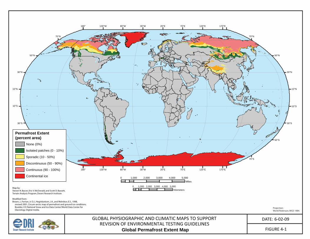
4.2.1 None (0%) Regions of the Earth centered near the equator between the latitudes of 25ºN and 25ºS
typically do not have any form of permafrost or ground ice. These regions are classified as
having no permafrost (0%) (Figure 4-1).
4.2.2 Isolated Patches (0 – 10%) High relief mountains or high and low interior plains between the latitudes of 60ºN
and 40ºN in the northern hemisphere and near the latitude of 50ºS in the southern hemisphere
that are neither covered by alpine glaciers, nor persist higher than ~15,000 ft (4600 m),
typically exhibit small pockets of permafrost. These regions are classified as having isolated
permafrost (0 – 10%) (Figure 4-1).
4.2.3 Sporadic (10 – 50%) High relief mountains at elevations above ~15,000 ft (4600 m) near the latitude of
30ºN in the Himalayan Mountains that are not covered by alpine glaciers or high and low
interior plains at much lower elevations near the latitude of 60ºN, typically exhibit variable
permafrost extent. These regions are classified as having sporadic permafrost (10 – 50%)
(Figure 4-1).
4.2.4 Discontinuous (50 – 90%) High relief mountains and plateaus at high elevations above ~15,000 ft (4600 m)
between the latitudes of 30ºN and 40ºN in the Himalayan Mountains and near 50ºN in
Mongolia and Siberia that are not covered by alpine glaciers or high and low interior plains at
much lower elevations between the latitudes of 60ºN and 70ºN exhibit an irregular mosaic of
permafrost. These regions are classified as having discontinuous permafrost (50 – 90%)
(Figure 4-1).
4.2.5 Continuous (90 – 100%) High and low interior plains at low elevations of the latitudes of 50ºN in Siberia and
50ºN and 60ºN in North America typically exhibit permanent permafrost. These regions are
classified as having continuous permafrost (90 – 100%) (Figure 4-1).
Final Report – July 6, 2009 21
Global Physiographic and Climatic Maps to Support Revision of Environmental Testing Guidelines
Final Report – July 6, 2009 22
4.2.6 Continental Ice Regions covered by extensive alpine glaciers and ice caps in Greenland and
Antarctica are classified as continental ice (Figure 4-1).
REVISION OF ENVIRONMENTAL TESTING GUIDELINESFIGURE 4-1
DATE: 6-02-09GLOBAL PHYSIOGRAPHIC AND CLIMATIC MAPS TO SUPPORT
Global Permafrost Extent Map
170°E
170°E
120°E
120°E
70°E
70°E
20°E
20°E
30°W
30°W
80°W
80°W
130°W
130°W
180°
180°
50°N 50°N
30°N 30°N
10°N 10°N
10°S 10°S
30°S 30°S
50°S
70°N 70°N
50°S
70°S 70°S
Projection: World Robinson, WGS 1984.
0 1,000 2,000 3,000 4,000 5,000Miles
0 1,000 2,000 3,000 4,000 5,000Kilometers
Map by: Steven N. Bacon, Eric V. McDonald, and Scott D. Bassett,Terrain Analysis Program, Desert Research Institute
Modified from:Brown, J., Ferrian, Jr. O.J., Heginbottom, J.A., and Melnikov, E.S., 1998, revised 2001, Circum-arctic map of permafrost and ground ice conditions. Boulder, CO: National Snow and Ice Data Center/World Data Center for Glaciology. Digital media.
Permafrost Extent(percent area)
None (0%)
Isolated patches (0 - 10%)
Sporadic (10 - 50%)
Discontinuous (50 - 90%)
Continuous (90 - 100%)
Continental ice
Global Physiographic and Climatic Maps to Support Revision of Environmental Testing Guidelines
Final Report – July 6, 2009 24
Table 5-1. Area distribution of global elevation breaks.
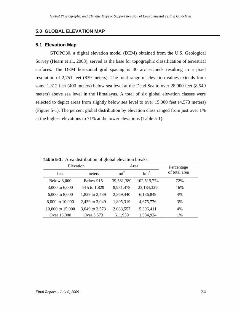
GTOPO30, a digital elevation model (DEM) obtained from the U.S. Geological
Survey (Hearn et al., 2003), served as the base for topographic classification of terrestrial
surfaces. The DEM horizontal grid spacing is 30 arc seconds resulting in a pixel
resolution of 2,751 feet (839 meters). The total range of elevation values extends from
some 1,312 feet (400 meters) below sea level at the Dead Sea to over 28,000 feet (8,540
meters) above sea level in the Himalayas. A total of six global elevation classes were
selected to depict areas from slightly below sea level to over 15,000 feet (4,573 meters)
(Figure 5-1). The percent global distribution by elevation class ranged from just over 1%
at the highest elevations to 71% at the lower elevations (Table 5-1).
5.1 Elevation Map
5.0 GLOBAL ELEVATION MAP
Elevation Area feet meters mi2 km2
Percentage of total area
Below 3,000 Below 915 39,581,380 102,515,774 72% 3,000 to 6,000 915 to 1,829 8,951,478 23,184,329 16% 6,000 to 8,000 1,829 to 2,439 2,369,440 6,136,849 4%
8,000 to 10,000 2,439 to 3,049 1,805,319 4,675,776 3% 10,000 to 15,000 3,049 to 3,573 2,083,557 5,396,411 4%
Over 15,000 Over 3,573 611,939 1,584,924 1%
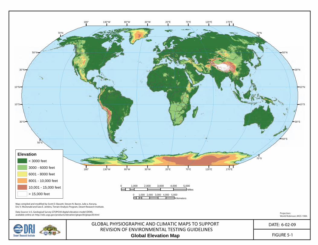
REVISION OF ENVIRONMENTAL TESTING GUIDELINESFIGURE 5-1
DATE: 6-02-09GLOBAL PHYSIOGRAPHIC AND CLIMATIC MAPS TO SUPPORT
Global Elevation Map
Projection: World Robinson, WGS 1984.
Map compiled and modified by Scott D. Bassett, Steven N. Bacon, Julie a. Koruna, Eric V. McDonald and Sara E. Jenkins, Terrain Analysis Program, Desert Research Institute.
Data Source: U.S. Geological Survey GTOPO30 digital elevation model (DEM), available online at: http://edc.usgs.gov/products/elevation/gtopo30/gtopo30.html
170°E
170°E
120°E
120°E
70°E
70°E
20°E
20°E
30°W
30°W
80°W
80°W
130°W
130°W
180°
180°
50°N 50°N
30°N 30°N
10°N 10°N
10°S 10°S
30°S 30°S
50°S
70°N 70°N
50°S
70°S 70°SElevation
< 3000 feet
3000 - 6000 feet
6001 - 8000 feet
8001 - 10,000 feet
10,001 - 15,000 feet
> 15,000 feet
0 1,000 2,000 3,000 4,000 5,000Miles
0 1,000 2,000 3,000 4,000 5,000Kilometers
Global Physiographic and Climatic Maps to Support Revision of Environmental Testing Guidelines
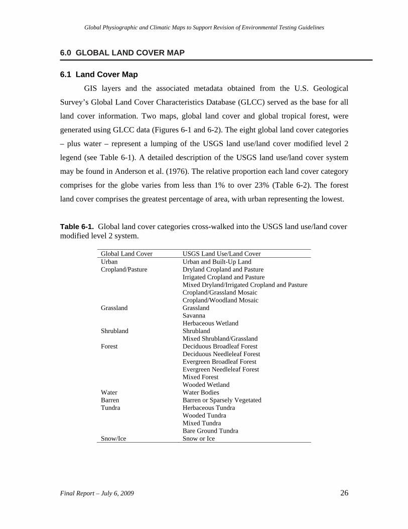
6.0 GLOBAL LAND COVER MAP
6.1 Land Cover Map GIS layers and the associated metadata obtained from the U.S. Geological
Survey’s Global Land Cover Characteristics Database (GLCC) served as the base for all
land cover information. Two maps, global land cover and global tropical forest, were
generated using GLCC data (Figures 6-1 and 6-2). The eight global land cover categories
– plus water – represent a lumping of the USGS land use/land cover modified level 2
legend (see Table 6-1). A detailed description of the USGS land use/land cover system
may be found in Anderson et al. (1976). The relative proportion each land cover category
comprises for the globe varies from less than 1% to over 23% (Table 6-2). The forest
land cover comprises the greatest percentage of area, with urban representing the lowest.
Table 6-1. Global land cover categories cross-walked into the USGS land use/land cover modified level 2 system.
Global Land Cover USGS Land Use/Land Cover Urban Urban and Built-Up Land Cropland/Pasture Dryland Cropland and Pasture Irrigated Cropland and Pasture Mixed Dryland/Irrigated Cropland and Pasture Cropland/Grassland Mosaic Cropland/Woodland Mosaic Grassland Grassland Savanna Herbaceous Wetland Shrubland Shrubland Mixed Shrubland/Grassland Forest Deciduous Broadleaf Forest Deciduous Needleleaf Forest Evergreen Broadleaf Forest Evergreen Needleleaf Forest Mixed Forest Wooded Wetland Water Water Bodies Barren Barren or Sparsely Vegetated Tundra Herbaceous Tundra Wooded Tundra Mixed Tundra Bare Ground Tundra Snow/Ice Snow or Ice
Final Report – July 6, 2009 26
Global Physiographic and Climatic Maps to Support Revision of Environmental Testing Guidelines
Final Report – July 6, 2009 27
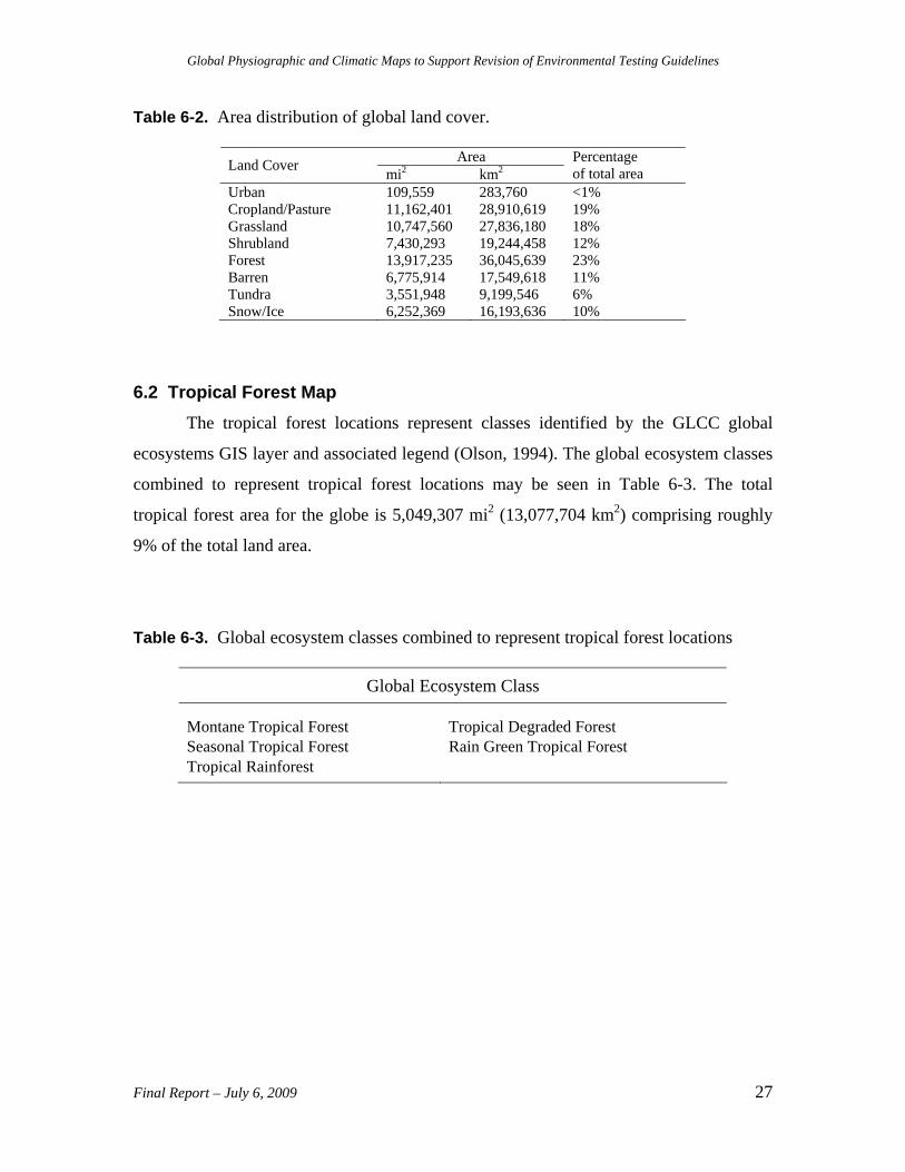
Table 6-2. Area distribution of global land cover.
Area Land Cover mi2 km2Percentage of total area
Urban 109,559 283,760 <1% Cropland/Pasture 11,162,401 28,910,619 19% Grassland 10,747,560 27,836,180 18% Shrubland 7,430,293 19,244,458 12% Forest 13,917,235 36,045,639 23% Barren 6,775,914 17,549,618 11% Tundra 3,551,948 9,199,546 6% Snow/Ice 6,252,369 16,193,636 10%
6.2 Tropical Forest Map The tropical forest locations represent classes identified by the GLCC global
ecosystems GIS layer and associated legend (Olson, 1994). The global ecosystem classes
combined to represent tropical forest locations may be seen in Table 6-3. The total
tropical forest area for the globe is 5,049,307 mi2 (13,077,704 km2) comprising roughly
9% of the total land area.
Table 6-3. Global ecosystem classes combined to represent tropical forest locations
Global Ecosystem Class
Montane Tropical Forest Tropical Degraded Forest Seasonal Tropical Forest Rain Green Tropical Forest Tropical Rainforest
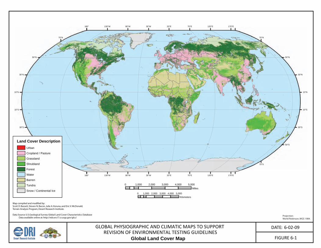
FIGURE 6-1
DATE: 6-02-09GLOBAL PHYSIOGRAPHIC AND CLIMATIC MAPS TO SUPPORTREVISION OF ENVIRONMENTAL TESTING GUIDELINES
Global Land Cover Map
170°E
170°E
120°E
120°E
70°E
70°E
20°E
20°E
30°W
30°W
80°W
80°W
130°W
130°W
180°
180°
50°N 50°N
30°N 30°N
10°N 10°N
10°S 10°S
30°S 30°S
50°S
70°N 70°N
50°S
70°S
Projection: World Robinson, WGS 1984.
0 1,000 2,000 3,000 4,000 5,000Miles
0 1,000 2,000 3,000 4,000 5,000Kilometers
Map compiled and modified by:Scott D. Bassett, Steven N. Bacon, Julie A. Koruna, and Eric V. McDonald,Terrain Analysis Program, Desert Research Institute.
Data Source: U.S.Geological Survey Global Land Cover Characteristics Database Data available online at: http://edcsns17.cr.usgs.gov/glcc/
Land Cover DescriptionUrban
Cropland / Pasture
Grassland
Shrubland
Forest
Water
Barren
Tundra
Snow / Continental Ice
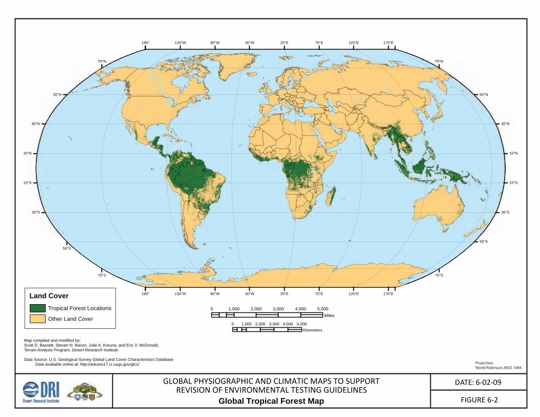
FIGURE 6-2
DATE: 6-02-09GLOBAL PHYSIOGRAPHIC AND CLIMATIC MAPS TO SUPPORTREVISION OF ENVIRONMENTAL TESTING GUIDELINES
Global Tropical Forest Map
170°E
170°E
120°E
120°E
70°E
70°E
20°E
20°E
30°W
30°W
80°W
80°W
130°W
130°W
180°
180°
50°N 50°N
30°N 30°N
10°N 10°N
10°S 10°S
30°S 30°S
50°S
70°N 70°N
50°S
70°S 70°S
Projection: World Robinson, WGS 1984.
0 1,000 2,000 3,000 4,000 5,000Miles
0 1,000 2,000 3,000 4,000 5,000Kilometers
Map compiled and modified by:Scott D. Bassett, Steven N. Bacon, Julie A. Koruna, and Eric V. McDonald,Terrain Analysis Program, Desert Research Institute.
Data Source: U.S. Geological Survey Global Land Cover Characteristics Database Data available online at: http://edcsns17.cr.usgs.gov/glcc/
Land CoverTropical Forest Locations
Other Land Cover
Global Physiographic and Climatic Maps to Support Revision of Environmental Testing Guidelines
7.0 GLOBAL CLIMATIC MAPS
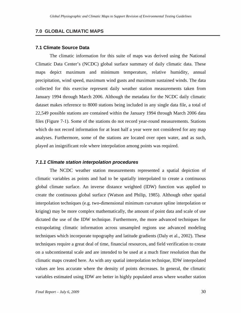
7.1 Climate Source Data The climatic information for this suite of maps was derived using the National
Climatic Data Center’s (NCDC) global surface summary of daily climatic data. These
maps depict maximum and minimum temperature, relative humidity, annual
precipitation, wind speed, maximum wind gusts and maximum sustained winds. The data
collected for this exercise represent daily weather station measurements taken from
January 1994 through March 2006. Although the metadata for the NCDC daily climatic
dataset makes reference to 8000 stations being included in any single data file, a total of
22,549 possible stations are contained within the January 1994 through March 2006 data
files (Figure 7-1). Some of the stations do not record year-round measurements. Stations
which do not record information for at least half a year were not considered for any map
analyses. Furthermore, some of the stations are located over open water, and as such,
played an insignificant role where interpolation among points was required.
7.1.1 Climate station interpolation procedures The NCDC weather station measurements represented a spatial depiction of
climatic variables as points and had to be spatially interpolated to create a continuous
global climate surface. An inverse distance weighted (IDW) function was applied to
create the continuous global surface (Watson and Philip, 1985). Although other spatial
interpolation techniques (e.g. two-dimensional minimum curvature spline interpolation or
kriging) may be more complex mathematically, the amount of point data and scale of use
dictated the use of the IDW technique. Furthermore, the more advanced techniques for
extrapolating climatic information across unsampled regions use advanced modeling
techniques which incorporate topography and latitude gradients (Daly et al., 2002). These
techniques require a great deal of time, financial resources, and field verification to create
on a subcontinental scale and are intended to be used at a much finer resolution than the
climatic maps created here. As with any spatial interpolation technique, IDW interpolated
values are less accurate where the density of points decreases. In general, the climatic
variables estimated using IDW are better in highly populated areas where weather station
Final Report – July 6, 2009 30
Global Physiographic and Climatic Maps to Support Revision of Environmental Testing Guidelines
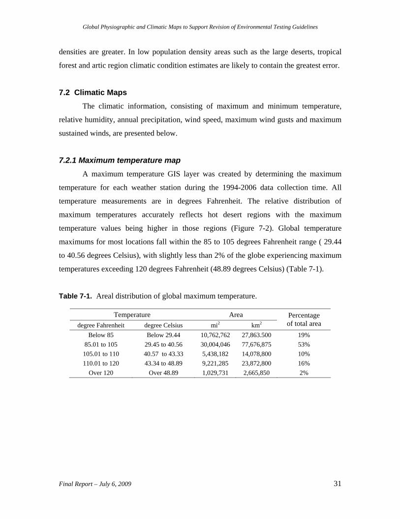
densities are greater. In low population density areas such as the large deserts, tropical
forest and artic region climatic condition estimates are likely to contain the greatest error.
7.2 Climatic Maps The climatic information, consisting of maximum and minimum temperature,
relative humidity, annual precipitation, wind speed, maximum wind gusts and maximum
sustained winds, are presented below.
7.2.1 Maximum temperature map A maximum temperature GIS layer was created by determining the maximum
temperature for each weather station during the 1994-2006 data collection time. All
temperature measurements are in degrees Fahrenheit. The relative distribution of
maximum temperatures accurately reflects hot desert regions with the maximum
temperature values being higher in those regions (Figure 7-2). Global temperature
maximums for most locations fall within the 85 to 105 degrees Fahrenheit range ( 29.44
to 40.56 degrees Celsius), with slightly less than 2% of the globe experiencing maximum
temperatures exceeding 120 degrees Fahrenheit (48.89 degrees Celsius) (Table 7-1).
Table 7-1. Areal distribution of global maximum temperature.
Temperature Area degree Fahrenheit degree Celsius mi2 km2
Percentage of total area
Below 85 Below 29.44 10,762,762 27,863.500 19% 85.01 to 105 29.45 to 40.56 30,004,046 77,676,875 53% 105.01 to 110 40.57 to 43.33 5,438,182 14,078,800 10% 110.01 to 120 43.34 to 48.89 9,221,285 23,872,800 16%
Over 120 Over 48.89 1,029,731 2,665,850 2%
Final Report – July 6, 2009 31
Global Physiographic and Climatic Maps to Support Revision of Environmental Testing Guidelines
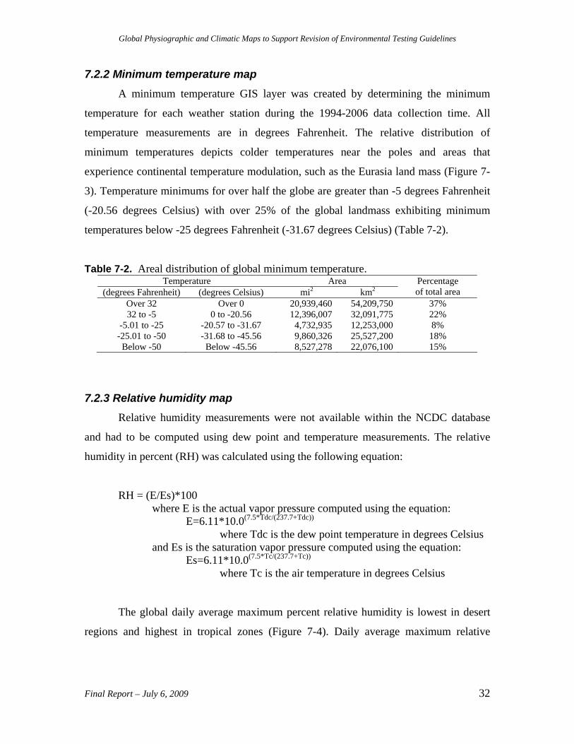
7.2.2 Minimum temperature map A minimum temperature GIS layer was created by determining the minimum
temperature for each weather station during the 1994-2006 data collection time. All
temperature measurements are in degrees Fahrenheit. The relative distribution of
minimum temperatures depicts colder temperatures near the poles and areas that
experience continental temperature modulation, such as the Eurasia land mass (Figure 7-
3). Temperature minimums for over half the globe are greater than -5 degrees Fahrenheit
(-20.56 degrees Celsius) with over 25% of the global landmass exhibiting minimum
temperatures below -25 degrees Fahrenheit (-31.67 degrees Celsius) (Table 7-2).
Table 7-2. Areal distribution of global minimum temperature. Temperature Area
(degrees Fahrenheit) (degrees Celsius) mi2 km2Percentage of total area
Over 32 Over 0 20,939,460 54,209,750 37% 32 to -5 0 to -20.56 12,396,007 32,091,775 22%
-5.01 to -25 -20.57 to -31.67 4,732,935 12,253,000 8% -25.01 to -50 -31.68 to -45.56 9,860,326 25,527,200 18% Below -50 Below -45.56 8,527,278 22,076,100 15%
7.2.3 Relative humidity map Relative humidity measurements were not available within the NCDC database
and had to be computed using dew point and temperature measurements. The relative
humidity in percent (RH) was calculated using the following equation:
RH = (E/Es)*100 where E is the actual vapor pressure computed using the equation:
E=6.11*10.0(7.5*Tdc/(237.7+Tdc))
where Tdc is the dew point temperature in degrees Celsius and Es is the saturation vapor pressure computed using the equation:
Es=6.11*10.0(7.5*Tc/(237.7+Tc))
where Tc is the air temperature in degrees Celsius
The global daily average maximum percent relative humidity is lowest in desert
regions and highest in tropical zones (Figure 7-4). Daily average maximum relative
Final Report – July 6, 2009 32
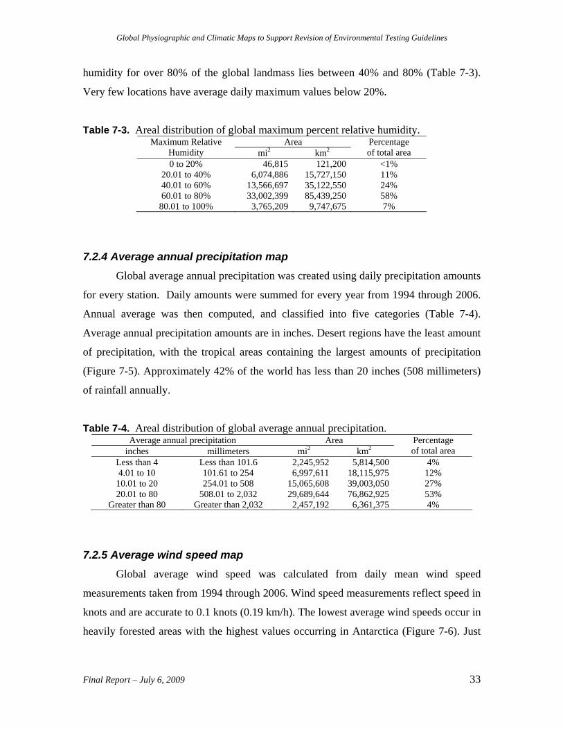
Global Physiographic and Climatic Maps to Support Revision of Environmental Testing Guidelines
humidity for over 80% of the global landmass lies between 40% and 80% (Table 7-3).
Very few locations have average daily maximum values below 20%.
Table 7-3. Areal distribution of global maximum percent relative humidity. Area Maximum Relative
Humidity mi2 km2Percentage of total area
0 to 20% 46,815 121,200 <1% 20.01 to 40% 6,074,886 15,727,150 11% 40.01 to 60% 13,566,697 35,122,550 24% 60.01 to 80% 33,002,399 85,439,250 58%
80.01 to 100% 3,765,209 9,747,675 7%
7.2.4 Average annual precipitation map Global average annual precipitation was created using daily precipitation amounts
for every station. Daily amounts were summed for every year from 1994 through 2006.
Annual average was then computed, and classified into five categories (Table 7-4).
Average annual precipitation amounts are in inches. Desert regions have the least amount
of precipitation, with the tropical areas containing the largest amounts of precipitation
(Figure 7-5). Approximately 42% of the world has less than 20 inches (508 millimeters)
of rainfall annually.
Table 7-4. Areal distribution of global average annual precipitation. Average annual precipitation Area
inches millimeters mi2 km2Percentage of total area
Less than 4 Less than 101.6 2,245,952 5,814,500 4% 4.01 to 10 101.61 to 254 6,997,611 18,115,975 12%
10.01 to 20 254.01 to 508 15,065,608 39,003,050 27% 20.01 to 80 508.01 to 2,032 29,689,644 76,862,925 53%
Greater than 80 Greater than 2,032 2,457,192 6,361,375 4%
7.2.5 Average wind speed map Global average wind speed was calculated from daily mean wind speed
measurements taken from 1994 through 2006. Wind speed measurements reflect speed in
knots and are accurate to 0.1 knots (0.19 km/h). The lowest average wind speeds occur in
heavily forested areas with the highest values occurring in Antarctica (Figure 7-6). Just
Final Report – July 6, 2009 33
Global Physiographic and Climatic Maps to Support Revision of Environmental Testing Guidelines
under 90% of the globe has average wind speeds below 10 knots (18.52 km/h) (Table 7-
5).
Table 7-5. Areal distribution of global average wind speed.
Average wind speed Area knots km/h mi2 km2
Percentage of total area
Less than 3 Less than 5.56 5,481,820 14,191,775 10% 3.01 to 10 5.57 to 18.52 44,254,697 114,570,100 78%
10.01 to 20 18.53 to 37.04 6,339,044 16,411,025 11% 20.01 to 40 37.05 to 74.08 349,389 904,525 1%
Greater than 40 Greater than 74.08 31,056 80,400 <1%
7.2.6 Wind gust map Global wind gusts were taken from daily wind gust measurements contained
within the 1994 through 2006 NCDC dataset described above. Wind gusts are defined as
“the maximum 3-second wind speed forecast to occur within a 2-minute interval at a
height of 10 meters”. Most of the globe experiences wind gusts above 34 knots (62.97
km/h) (Figure 7-7). The categories selected to represent wind gust breaks approximate
wind speeds under which specific kinds of damage to structures or vegetation are
probable. For instance, wind gusts that exceed 63 knots (116.67 km/h) are indicative of
hurricane devastation (see Table 7-6). The relative contribution of the gust speed classes
by global area ranges from less than 1% to 69% (Table 7-7).
Table 7-6. Generalized wind speed description for five selected categories.
Wind speed knots km/h
Description
Less than 6 Less than 11.11 Light breeze, wind felt 6.01 to 19 11.12 to 35.19 Light breeze, leaves begin to sway
19.01 to 34 35.20 to 62.97 Moderate gale, inconvenience in walking 34.01 to 63 62.98 to 116.67 Strong gale, trees losing limbs or uprooting
Greater than 63 Greater than 116.67 Hurricane force winds
Final Report – July 6, 2009 34
Global Physiographic and Climatic Maps to Support Revision of Environmental Testing Guidelines
Final Report – July 6, 2009 35
Table 7-7. Areal distribution of global maximum wind gusts.
Wind speed Area knots km/h mi2 km2
Percentage of total area
Less than 6 Less than 11.11 12,505 32,375 <1% 6.01 to 19 11.12 to 35.19 1,118,824 2,896,500 2%
19.01 to 34 35.20 to 62.97 9,172,219 23,745,775 16% 34.01 to 63 62.98 to 116.67 38,739,098 100,290,875 69%
Greater than 63 Greater than 116.67 7,284,810 18,859,500 13%
7.2.7 Maximum sustained winds map Global maximum sustained wind speeds were taken from daily sustained wind
speed measurements contained within the 1994 through 2006 NCDC dataset described
above. Sustained wind speeds are calculated by the National Hurricane Center using a
one minute moving average, thus reflecting the maximum average wind speed which
occurs for any single minute during a single day. Most of the global landmass
experiences maximum sustained wind speeds above 34 knots (62.97 km/h) (Figure 7-8).
The wind gust table description for wind speeds has the same categorization and
descriptions for maximum sustained wind speed classes (Table 7-8). The relative
contribution of the wind speed classes by global area ranges from less than 1% to 74%
(Table 7-8).
Table 7-8. Area distribution of global maximum sustained winds.
Wind speed Area knots km/h mi2 km2
Percentage of total area
Less than 6 Less than 11.11 27,202 70,425 <1% 6.01 to 19 11.12 to 35.19 2,004,149 5,188,500 4%
19.01 to 34 35.20 to 62.97 8,887,279 23,008,100 16% 34.01 to 63 62.98 to 116.67 42,049,100 108,860,075 74%
Greater than 63 Greater than 116.67 3,488,275 9,030,725 6%
FIGURE 7-1
DATE: 6-02-09GLOBAL PHYSIOGRAPHIC AND CLIMATIC MAPS TO SUPPORTREVISION OF ENVIRONMENTAL TESTING GUIDELINES
Global Distribution of Weather Stations
170°E
170°E
120°E
120°E
70°E
70°E
20°E
20°E
30°W
30°W
80°W
80°W
130°W
130°W
180°
180°
50°N 50°N
30°N 30°N
10°N 10°N
10°S 10°S
30°S 30°S
50°S
70°N 70°N
50°S
70°S 70°S
Projection: World Robinson, WGS 1984.
0 1,000 2,000 3,000 4,000 5,000Miles
0 1,000 2,000 3,000 4,000 5,000Kilometers
LegendWeather Station
Map compiled and modified by Scott D. Bassett, Steven N. Bacon, Julie A. Koruna, and Eric V. McDonald, Terrain Analysis Program, Desert Research Institute.
Data Source: 1994-2006 NCDC/NOAA Global Surface Summary Worldwide Stations available online at: ftp.ncdc.noaa.gov/pub/data/globalsod
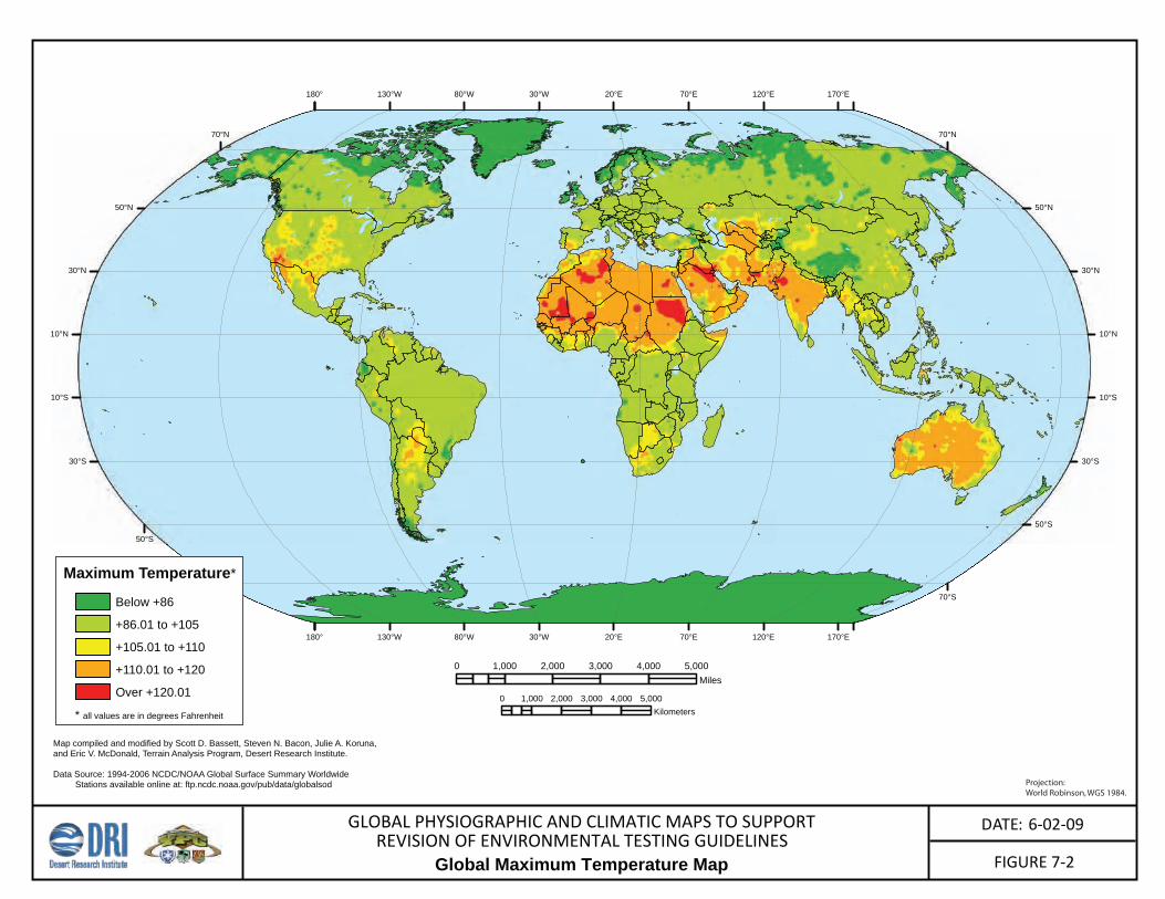
FIGURE 7-2
DATE: 6-02-09GLOBAL PHYSIOGRAPHIC AND CLIMATIC MAPS TO SUPPORTREVISION OF ENVIRONMENTAL TESTING GUIDELINES
Global Maximum Temperature Map
170°E
170°E
120°E
120°E
70°E
70°E
20°E
20°E
30°W
30°W
80°W
80°W
130°W
130°W
180°
180°
50°N 50°N
30°N 30°N
10°N 10°N
10°S 10°S
30°S 30°S
50°S
70°N 70°N
50°S
70°S 70°S
Projection: World Robinson, WGS 1984.
0 1,000 2,000 3,000 4,000 5,000Miles
0 1,000 2,000 3,000 4,000 5,000Kilometers
Maximum Temperature*
Map compiled and modified by Scott D. Bassett, Steven N. Bacon, Julie A. Koruna, and Eric V. McDonald, Terrain Analysis Program, Desert Research Institute.
Data Source: 1994-2006 NCDC/NOAA Global Surface Summary Worldwide Stations available online at: ftp.ncdc.noaa.gov/pub/data/globalsod
* all values are in degrees Fahrenheit
Below +86
+86.01 to +105
+105.01 to +110
+110.01 to +120
Over +120.01
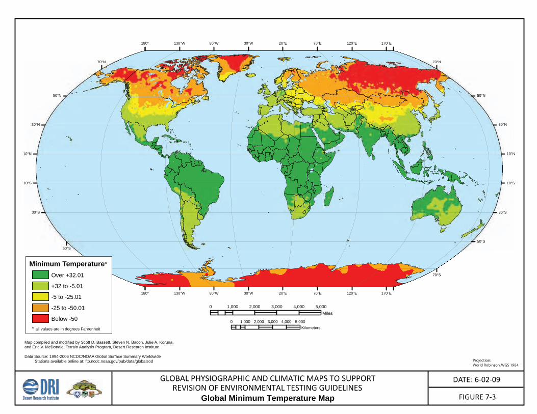
FIGURE 7-3
DATE: 6-02-09GLOBAL PHYSIOGRAPHIC AND CLIMATIC MAPS TO SUPPORTREVISION OF ENVIRONMENTAL TESTING GUIDELINES
Global Minimum Temperature Map
170°E
170°E
120°E
120°E
70°E
70°E
20°E
20°E
30°W
30°W
80°W
80°W
130°W
130°W
180°
180°
50°N 50°N
30°N 30°N
10°N 10°N
10°S 10°S
30°S 30°S
50°S
70°N 70°N
50°S
70°S 70°S
Projection: World Robinson, WGS 1984.
0 1,000 2,000 3,000 4,000 5,000Miles
0 1,000 2,000 3,000 4,000 5,000Kilometers
Minimum Temperature*
Map compiled and modified by Scott D. Bassett, Steven N. Bacon, Julie A. Koruna, and Eric V. McDonald, Terrain Analysis Program, Desert Research Institute.
Data Source: 1994-2006 NCDC/NOAA Global Surface Summary Worldwide Stations available online at: ftp.ncdc.noaa.gov/pub/data/globalsod
* all values are in degrees Fahrenheit
Over +32.01
+32 to -5.01
-5 to -25.01
-25 to -50.01
Below -50
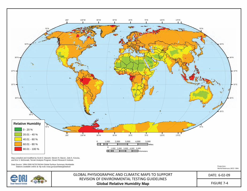
FIGURE 7-4
DATE: 6-02-09GLOBAL PHYSIOGRAPHIC AND CLIMATIC MAPS TO SUPPORTREVISION OF ENVIRONMENTAL TESTING GUIDELINES
Global Relative Humidity Map
170°E
170°E
120°E
120°E
70°E
70°E
20°E
20°E
30°W
30°W
80°W
80°W
130°W
130°W
180°
180°
50°N 50°N
30°N 30°N
10°N 10°N
10°S 10°S
30°S 30°S
50°S
70°N 70°N
50°S
70°S 70°S
Projection: World Robinson, WGS 1984.
0 1,000 2,000 3,000 4,000 5,000Miles
0 1,000 2,000 3,000 4,000 5,000Kilometers
Relative Humidity
Map compiled and modified by Scott D. Bassett, Steven N. Bacon, Julie A. Koruna, and Eric V. McDonald, Terrain Analysis Program, Desert Research Institute.
Data Source: 1994-2006 NCDC/NOAA Global Surface Summary Worldwide Stations available online at: ftp.ncdc.noaa.gov/pub/data/globalsod
0 - 20 %
20.01 - 40 %
40.01 - 60 %
60.01 - 80 %
80.01 - 100 %
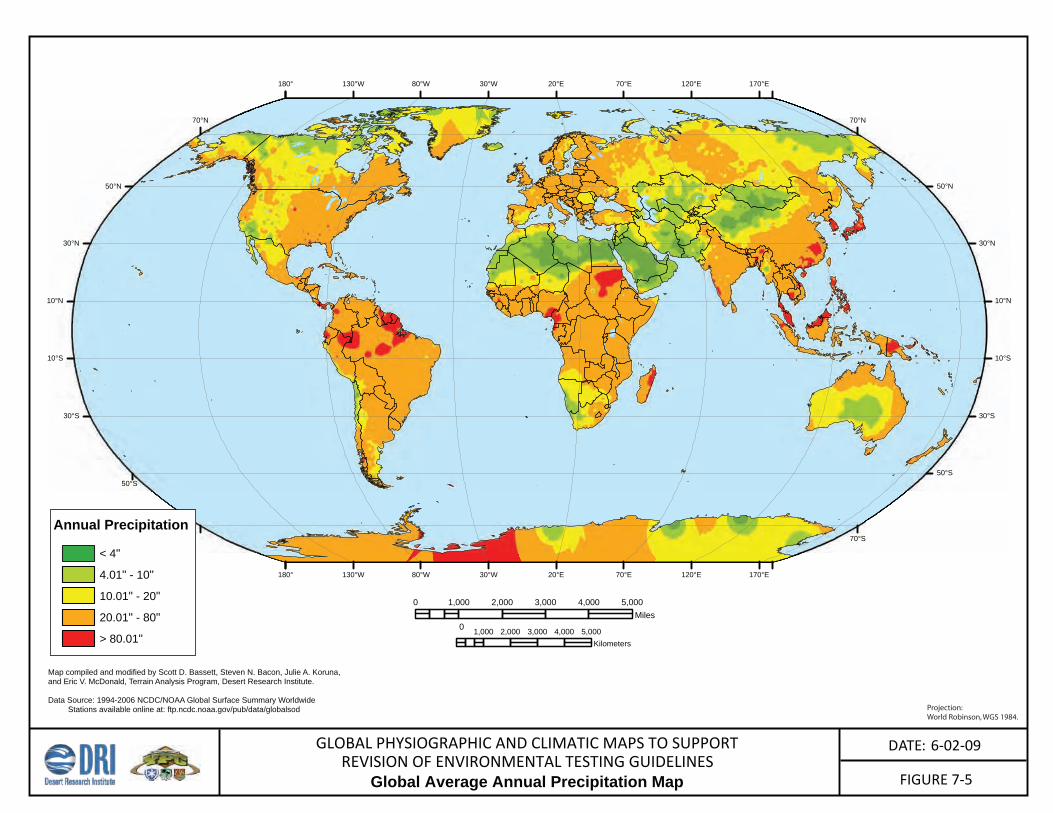
FIGURE 7-5
DATE: 6-02-09GLOBAL PHYSIOGRAPHIC AND CLIMATIC MAPS TO SUPPORTREVISION OF ENVIRONMENTAL TESTING GUIDELINES
Global Average Annual Precipitation Map
170°E
170°E
120°E
120°E
70°E
70°E
20°E
20°E
30°W
30°W
80°W
80°W
130°W
130°W
180°
180°
50°N 50°N
30°N 30°N
10°N 10°N
10°S 10°S
30°S 30°S
50°S
70°N 70°N
50°S
70°S
Projection: World Robinson, WGS 1984.
0 1,000 2,000 3,000 4,000 5,000Miles
0 1,000 2,000 3,000 4,000 5,000Kilometers
Annual Precipitation
Map compiled and modified by Scott D. Bassett, Steven N. Bacon, Julie A. Koruna, and Eric V. McDonald, Terrain Analysis Program, Desert Research Institute.
Data Source: 1994-2006 NCDC/NOAA Global Surface Summary Worldwide Stations available online at: ftp.ncdc.noaa.gov/pub/data/globalsod
< 4"
4.01" - 10"
10.01" - 20"
20.01" - 80"
> 80.01"
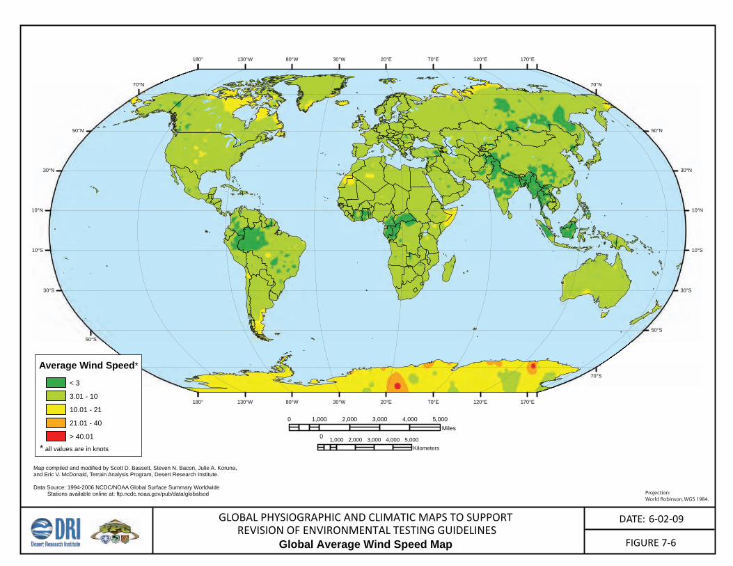
FIGURE 7-6
DATE: 6-02-09GLOBAL PHYSIOGRAPHIC AND CLIMATIC MAPS TO SUPPORTREVISION OF ENVIRONMENTAL TESTING GUIDELINES
Global Average Wind Speed Map
170°E
170°E
120°E
120°E
70°E
70°E
20°E
20°E
30°W
30°W
80°W
80°W
130°W
130°W
180°
180°
50°N 50°N
30°N 30°N
10°N 10°N
10°S 10°S
30°S 30°S
50°S
70°N 70°N
50°S
70°S
Projection: World Robinson, WGS 1984.
0 1,000 2,000 3,000 4,000 5,000Miles
0 1,000 2,000 3,000 4,000 5,000Kilometers
Average Wind Speed*
Map compiled and modified by Scott D. Bassett, Steven N. Bacon, Julie A. Koruna, and Eric V. McDonald, Terrain Analysis Program, Desert Research Institute.
Data Source: 1994-2006 NCDC/NOAA Global Surface Summary Worldwide Stations available online at: ftp.ncdc.noaa.gov/pub/data/globalsod
* all values are in knots
< 3
3.01 - 10
10.01 - 21
21.01 - 40
> 40.01
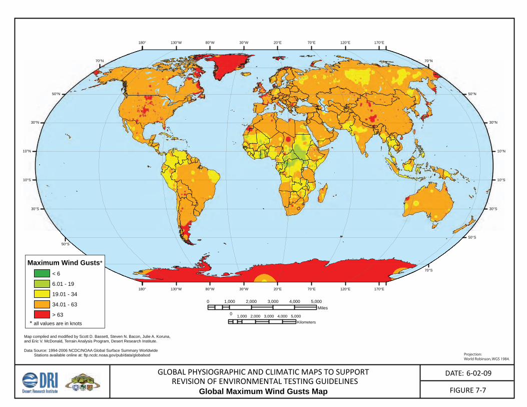
FIGURE 7-7
DATE: 6-02-09GLOBAL PHYSIOGRAPHIC AND CLIMATIC MAPS TO SUPPORTREVISION OF ENVIRONMENTAL TESTING GUIDELINES
Global Maximum Wind Gusts Map
170°E
170°E
120°E
120°E
70°E
70°E
20°E
20°E
30°W
30°W
80°W
80°W
130°W
130°W
180°
180°
50°N 50°N
30°N 30°N
10°N 10°N
10°S 10°S
30°S 30°S
50°S
70°N 70°N
50°S
70°S 70°S
Projection: World Robinson, WGS 1984.
0 1,000 2,000 3,000 4,000 5,000Miles
0 1,000 2,000 3,000 4,000 5,000Kilometers
Maximum Wind Gusts*
Map compiled and modified by Scott D. Bassett, Steven N. Bacon, Julie A. Koruna, and Eric V. McDonald, Terrain Analysis Program, Desert Research Institute.
Data Source: 1994-2006 NCDC/NOAA Global Surface Summary Worldwide Stations available online at: ftp.ncdc.noaa.gov/pub/data/globalsod
* all values are in knots
< 6
6.01 - 19
19.01 - 34
34.01 - 63
> 63
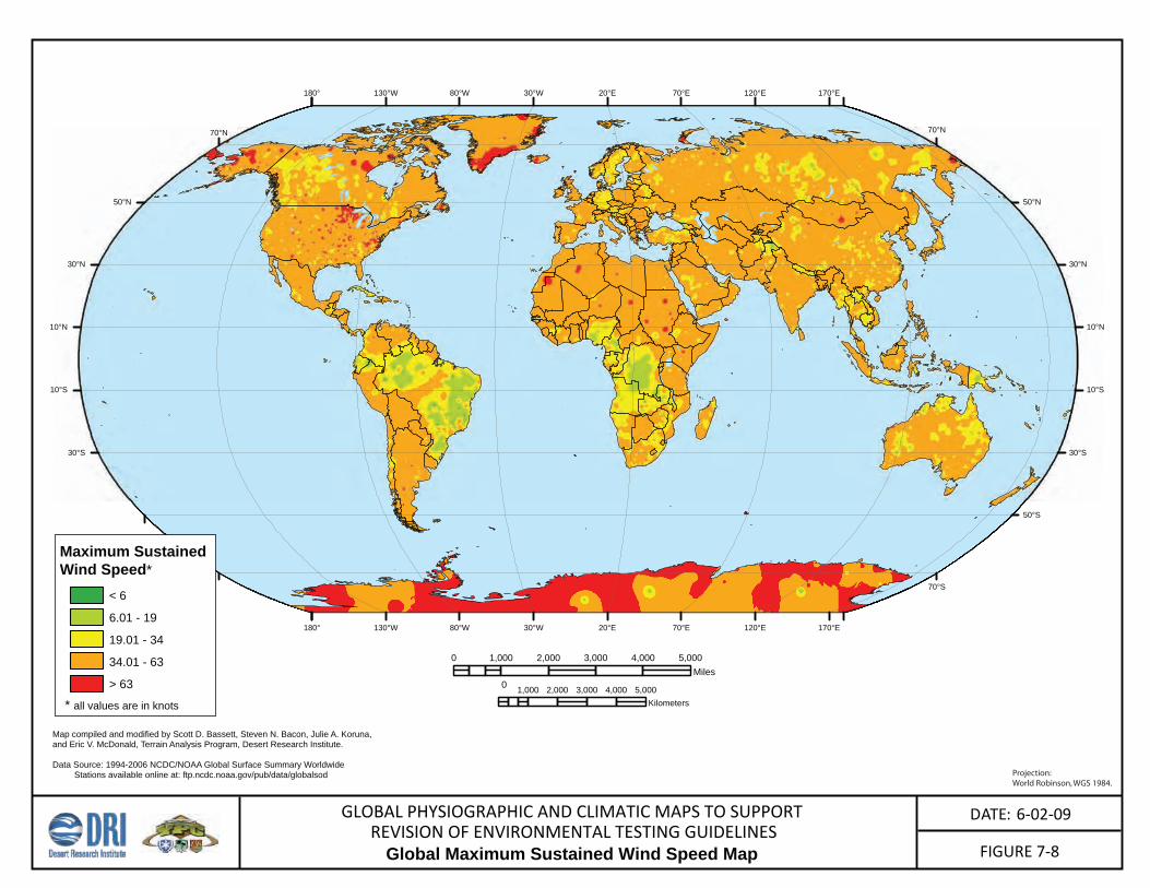
FIGURE 7-8
DATE: 6-02-09GLOBAL PHYSIOGRAPHIC AND CLIMATIC MAPS TO SUPPORTREVISION OF ENVIRONMENTAL TESTING GUIDELINES
Global Maximum Sustained Wind Speed Map
170°E
170°E
120°E
120°E
70°E
70°E
20°E
20°E
30°W
30°W
80°W
80°W
130°W
130°W
180°
180°
50°N 50°N
30°N 30°N
10°N 10°N
10°S 10°S
30°S 30°S
50°S
70°N 70°N
70°S
Projection: World Robinson, WGS 1984.
0 1,000 2,000 3,000 4,000 5,000Miles
0 1,000 2,000 3,000 4,000 5,000Kilometers
Maximum SustainedWind Speed*
Map compiled and modified by Scott D. Bassett, Steven N. Bacon, Julie A. Koruna, and Eric V. McDonald, Terrain Analysis Program, Desert Research Institute.
Data Source: 1994-2006 NCDC/NOAA Global Surface Summary Worldwide Stations available online at: ftp.ncdc.noaa.gov/pub/data/globalsod
* all values are in knots
< 6
6.01 - 19
19.01 - 34
34.01 - 63
> 63
Global Physiographic and Climatic Maps to Support Revision of Environmental Testing Guidelines
8.0 REFERENCES
Anderson, J.R., Hardy, E.E., Roach, J.T., and Witmer, R.E., 1976. A land use and land cover classification system for use with remote sensor data. U.S. Geological Survey Professional Paper 964, 28 pp.
Bailey, R.G., 1998. Ecoregions: The Ecosystem Geography of the Oceans and
Continents. Springer-Verlag, Inc., New York: 176 pp. Barton, K.E., Howell, D.G., and Vigil, J.F., 2003. The North American tapestry of time
and terrain. U.S. Geological Survey, Geologic Investigation Series I-2781. (map scale: 1:8,000,000).
Bates, R.L., and Jackson, J.A., (eds.), 1987. Glossary of Geology: American Geological
Institute, Alexandria, VA, 3rd edition, 788 pp. © 2003 American Geological Institute.
Bostock, H.S., 1967. Physiographic regions. The national atlas of Canada. (map scale:
1:15,000,000). Brown, J., Ferrians, O.J., Jr., Heginbottom, J.A., and Melnikov, E.S., 1998 (revised
2001). Circum-arctic map of permafrost and ground ice conditions. Boulder, CO: National Snow and Ice Data Center for Glaciology. Digital media.
Busacca, A.J., and Sweeney, M.R., 2005. Loess. In: Hill, D., (ed.), Encyclopedia of soils
in the environment. Academic Press, p. 364-373. Daly, C., Gibson, W.P., Taylor, G.H., Johnson, G.L., Pasteris, P., 2002. A knowledge-
based approach to the statistical mapping of climate. Climate Research, v. 22, p. 99-113.
FAO [Food and Agriculture Organization], 1999. Soil and physiographic database for
north and central Eurasia 1:5,000,000. [CD-ROM]. FAO land and water digital media series #07. Version 1.0 for Windows. UNESCO, Paris.
FAO-UNESCO-ISRIC, 1988. Revised legend of the soil map of the World. World Soil
Resources Report n0 06. FAO, Rome Italy. FAO-UNESCO-ISRIC, 1990. Revised legend of the soil map of the World. World Soil
Resources Report n0 06. FAO, Rome Italy. FAO-UNESCO-ISRIC, 1998. World reference base for soil resources. World Resources
Report, #84. FAO, Rome, 88 pp.
Final Report – July 6, 2009 44
Global Physiographic and Climatic Maps to Support Revision of Environmental Testing Guidelines
Hammond, E.H., 1954. Small-Scale Continental Landform Maps. Annals of the Association of American Geographers, v. 44, p. 33-42.
Hearn, P., Hare, T., Schruben, P., Sherrill, D., LaMar, C., and Tsushima, P., 2003. Global
GIS, A Digital Atlas of Planet Earth, Digital Data Series DDS-62 A-H, U.S. Geological Survey.
McDonald, E.V., Bacon, S.N., Bassett, S.D., and Jenkins, S.E., 2009. Catalog of
Analogs: Terrain Similarities between the U.S. Army Yuma Proving Ground and central southwest Asia – Final Report, Prepared for U.S. Army Yuma Proving Ground, Natural Environments Test Office by Desert Research Institute. May 21, 2009, 95 pp.
Nachtergaele, F.O., Spaargaren, O., Deckers, J.A., Ahrens, B., 2000. New developments
in soil classification World Reference Base for Soil Resources. Geoderma, v. 96, p. 345-357.
Olson, J.S., 1994. Global ecosystem framework-definitions. USGS EROS Data Center
Ineternal Report, Sioux Falls, SD., 38 pp. Permafrost subcommittee, 1998, Glossary of permafrost and related ground ice terms.
National Research Council of Canada. Technical memorandum, No. 142, 156 pp. Pidwirny, M., 2006. Fundamentals of Physical Geography, 2nd Edition. November, 16.
http://www.physicalgeography.net/fundamentals/contents.htm. Soil Survey Staff, 1999. Soil Taxonomy: A Basic System of Soil Classification for
Making and Interpreting Soil Surveys, Second Edition. USDA Handbook Number 436.
Wilson, D.F. Philip, G.M., 1985. A refinement of inverse distance weighted interpolation.
Geo-Processing, v. 2, p. 315-327.
Final Report – July 6, 2009 45