energies

Article

Global Maximum Power Point Tracking (MPPT) ofa Photovoltaic Module Array Constructed throughImproved Teaching-Learning-Based Optimization

Kuei-Hsiang Chao * and Meng-Cheng Wu

Department of Electrical Engineering, National Chin-Yi University of Technology, Taichung 41170, Taiwan;kamp7749@gmail.com* Correspondence: chaokh@ncut.edu.tw; Tel.: +886-4-2392-4505 (ext. 7272); Fax: +886-4-2392-2156

Academic Editors: Senthilarasu Sundaram and Tapas MallickReceived: 10 September 2016; Accepted: 15 November 2016; Published: 25 November 2016

Abstract: The present study proposes a maximum power point tracking (MPPT) method in whichimproved teaching-learning-based optimization (I-TLBO) is applied to perform global MPPT ofphotovoltaic (PV) module arrays under dissimilar shading situations to ensure the maximum poweroutput of the module arrays. The proposed I-TLBO enables the automatic adjustment of teachingfactors according to the self-learning ability of students. Incorporating smart-tracking and self-studystrategies can effectively improve the tracking response speed and steady-state tracking performance.To evaluate the feasibility of the proposed I-TLBO, a HIP-2717 PV module array from Sanyo Electricwas employed to compose various arrays with different serial and parallel configurations. The arrayswere operated under different shading conditions to test the MPPT with double, triple, or quadruplepeaks of power-voltage characteristic curves. Boost converters were employed with TMS320F2808digital signal processors to test the proposed MPPT method. Empirical results confirm that theproposed method exhibits more favorable dynamic and static-state response tracking performancecompared with that of conventional TLBO.

Keywords: maximum power point tracking; teaching-learning-based optimization; photovoltaicmodule array; partial module shading

1. Introduction

A photovoltaic (PV) power generation system is composed of a PV module array, a powerconditioner, and a power transmission and distribution system. Because the output power of a PVmodule array changes substantially under the effect of insolation and environmental temperaturechanges [1], power conditioners not only function as inverters, but also require a maximum powerpoint (MPP) tracker to control the PV module array. Consequently, power loss in the PV module arraycan be reduced while maintaining MPP output under different environmental conditions.

Different sets of power–voltage (P–V) characteristic curves can be generated for differentinsolation and environmental temperature. To ensure the maximum power output, the duty cycles ofa power converter are commonly adopted. Concerning conventional maximum power point tracking(MPPT) techniques, they include the most frequently adopted perturb and observe (P&O) [2–4] andincremental conductance (INC) [5,6] methods. Although the P&O method is simple and involvesonly a few parameters, a drawback of this method is that users must choose between tracking speedand number of oscillations, in which favorable performance of one comes at the expense of the other.By contrast, the INC method improves tracking speed but features unfavorable tracking stabilitybecause precision sensors are required to measure the conductance. Moreover, when PV array modulesare faulty or subjected to partial shading, the corresponding P–V characteristic curves exhibit multiple

Energies 2016, 9, 986; doi:10.3390/en9120986 www.mdpi.com/journal/energies

Energies 2016, 9, 986 2 of 18

peaks [7]. Thus, applying these two conventional MPPT methods generates local MPPs rather thanglobal MPPs. Shaded modules in a PV array are known to incur mismatching problems. In this context,the global MPP cannot be successfully tracked using a typical Field MPPT, that is to say, deterioratedpower generation efficiency, due to the multiple peaks on a P–V characteristic curve. A distributedmaximum power point tracker (DMPPT) was proposed as a way to resolve this mismatching problemand hence to elevate the overall power generation efficiency [8,9]. However, a clear disadvantage ofa DMPP tracker is a rise in the cost and more room occupied. For this sake, to develop a low cost, buthigh performance, global MPP tracker to deal with the multi-peak problems on a P–V characteristiccurve for the optimal performance of a PV array is an important research effort.

In recent years, numerous scholars have investigated MPPT methods for PV module arraysexhibiting multiple peaks under partial shading. Commonly adopted intelligent algorithms includethe differential evolution (DE) [10], the ant colony optimization (ACO) [11], and the artificial beecolony (ABC) algorithms [12]. The DE algorithm, similar to a genetic algorithm [13,14], performs realnumber coding on selected groups to search for a global optimal solution through the differentialcalculation of variance and one-to-one competitive survival strategies. However, as demonstratedin [15], only simulation results were presented. In addition, individual mutation strategies werebased on a total of five equations proposed by Storn [16], which not only increases tracking-timecalculations, but also requires a more accurate comparison between population codes during crossovercoding with microcontrollers. The ACO algorithm is a probabilistic path optimization algorithmbased on the foraging behaviors of ants. The pheromones that ants lay down when they find food areused as a food-source indicator, with which other ants can determine the optimal food-finding path;this conserves time otherwise spent on random searching. In [17], pheromone update equationswere expressed as exponential functions that yielded random values for transitioning betweencontrolling the pheromone density and path length. Although this approach eliminates the possibilityof identifying local optimal solutions, calculating the path length by using exponential functionsrequires considerably longer tracking time. The ABC algorithm transmits information regarding thequality and position of a food source through the “dance” performed by employed bees, which areresponsible for finding larger food sources to increase profitability during the colony food-findingoptimization process [18]. However, the employed bee phase relies on random values, resulting inan unstable searching capacity. In addition, in the scout phase, the number of bees selected affectsthe tracking speed and steady-state performance. As mentioned in [18], obtaining the statisticalresults of ABC and particle swarm optimization (PSO) algorithms requires 5–6 s, indicating thatthe tracking response speed can be improved. Moreover, scholars have proposed incorporatingintelligent algorithms with conventional MPPT algorithms [19–22], such as incorporating PSO orgenetic algorithms with P&O. Although the incorporated methods can successfully identify globaloptimal solutions, the dynamic response speed is too slow.

To address these problems, the present study incorporated a novel teaching-learning-basedoptimization (TLBO) method [23,24] to track the MPPs of a PV module array subjected to partialshading. The proposed method is advantageous because of its independence from populationoptimization, high adaptability, few design parameters, simple algorithm, and ease of understanding.In the present study, a conventional TLBO algorithm [25] was modified to improve the convergenceand reduce the tracking time to obtain a more efficient algorithm than extant MPPT algorithms.The proposed algorithm improves MPPT tracking effectiveness for PV module arrays exhibitingmultiple peaks in their P–V characteristic curves.

2. Fault and Shading Characteristics of PV Module Arrays

To increase the power output of a PV power generation system, PV modules are generallycombined in serial and parallel configurations. However, external environments can cause shadingbecause of dust, stains, and tall buildings, which generates nonlinear changes and multiple peaks inP–V characteristic curves. To examine the P–V and I–V output characteristics of serial and parallel

Energies 2016, 9, 986 3 of 18

PV module arrays subjected to partial shading, the SANYO HIP 2717 module [26] was adopted andvarious shading ratios were used. In addition, various arrays of serial and parallel configurations weretested. Table 1 lists the electricity parameter specifications of a single module under standard testconditions (i.e., air mass of 1.5, irradiance of 1000 W/m2, and PV module temperature of 25 ◦C) [26].

Table 1. Electricity parameter specifications of the SANYO HIP 2717 PV module.

Parameter Value

Rated maximum power output (Pmp) 27.8 WMPP current (Imp) 1.63 AMPP voltage (Vmp) 17.1 V

Short-circuit current (Isc) 1.82 AOpen-circuit voltage (Voc) 21.6 V

Module dimensions 496 mm × 524 mm

2.1. PV Module Simulator Circuit

The present study adopted the circuit of a PV module simulator with adjustable shading ratios [27],as shown in Figure 1. The circuit structure primarily comprises a Darlington amplifier, a currentlimiting circuit, and a voltage regulator for attaining PV module output characteristics under varyingshading ratios, which were created by adjusting variable resistors VRIsc and VRVoc. The variableresistor VRVoc shown in Figure 1 controls the open-circuit voltage of the PV module. When the circuitis open, a current-limiting transistor Q3 is operated at the cutoff region. The open-circuit voltage iscalculated using Equation (1):

Voc = VPV −VCE2 −VDBlocking (1)

Short-circuit currents can be calculated by adjusting VRIsc to operate the current limiting transistorQ3 at the saturation region when the VBE3 voltage drop crosses over RD. The short-circuit current iscalculated using Equation (2):

Isc = I = VBE3 ×RD + VRISC

RD × RC(2)

If the VPV power source is not provided, the PV module simulator generates zero power output,which is equivalent to the fault situation of the PV module. Using a bypass diode DBypass can ensure thatPV module arrays generate a certain amount of power during fault events. Accordingly, the electricityparameters of PV modules can be employed to set the required PV module output characteristics.

Energies 2016, 9, 986 3 of 18

were tested. Table 1 lists the electricity parameter specifications of a single module under standard

test conditions (i.e., air mass of 1.5, irradiance of 1000 W/m2, and PV module temperature of 25 °C)

[26].

Table 1. Electricity parameter specifications of the SANYO HIP 2717 PV module.

Parameter Value

Rated maximum power output (Pmp) 27.8 W

MPP current (Imp) 1.63 A

MPP voltage (Vmp) 17.1 V

Short-circuit current (Isc) 1.82 A

Open-circuit voltage (Voc) 21.6 V

Module dimensions 496 mm × 524 mm

2.1. PV Module Simulator Circuit

The present study adopted the circuit of a PV module simulator with adjustable shading ratios

[27], as shown in Figure 1. The circuit structure primarily comprises a Darlington amplifier, a current

limiting circuit, and a voltage regulator for attaining PV module output characteristics under varying

shading ratios, which were created by adjusting variable resistors VRIsc and VRVoc. The variable

resistor VRVoc shown in Figure 1 controls the open-circuit voltage of the PV module. When the circuit

is open, a current-limiting transistor Q3 is operated at the cutoff region. The open-circuit voltage is

calculated using Equation (1):

2 Blockingoc PV CE DV V V V (1)

Short-circuit currents can be calculated by adjusting VRIsc to operate the current limiting

transistor Q3 at the saturation region when the VBE3 voltage drop crosses over RD. The short-circuit

current is calculated using Equation (2):

3D ISC

sc BE

D C

R VRI I V

R R

(2)

If the VPV power source is not provided, the PV module simulator generates zero power output,

which is equivalent to the fault situation of the PV module. Using a bypass diode DBypass can ensure

that PV module arrays generate a certain amount of power during fault events. Accordingly, the

electricity parameters of PV modules can be employed to set the required PV module output

characteristics.

PVV

AR

4BEV

4Q

VocVR

BR

1Q

2Q

2CEV

3Q

3BEV

SCIVR

DR

DRV

CRV

BlockingD

BlockingDV

BypassD

IC

R

Load

Figure 1. PV module simulator circuit.

Figure 1. PV module simulator circuit.

Energies 2016, 9, 986 4 of 18

2.2. PV Module Array Fault and Shading Characteristics Analysis

2.2.1. PV Module Array Characteristics without Faults or Shading

When a PV module array has M serial and N parallel arrays without shading or faults and theMPP voltage, MPP current, and MPP power are respectively denoted as Vmp, Imp, and Pmp, the MPPvoltage, MPP current, and MPP power of the M serial and N parallel arrays are expressed as M × Vmp,N × Imp, and M × N × Pmp, respectively.

2.2.2. PV Module Array Characteristics with Faults or Shading

In a PV module array, fault or shading incidences in a module can decrease the power output ofthe array. Similar to an actual module, a PV module simulator enables a fault module to form a loopthrough a bypass diode. Using a bypass diode not only ensures that the PV module array maintainsa certain level of power generation, but that it also has little effect on the MPPT. However, when themodule is under partial shading, the output voltage and current decrease, causing multiple peaks inthe P–V characteristic curves of the PV module array, which prevents conventional MPP trackers fromcontrolling the module array to operate at the actual MPPs.

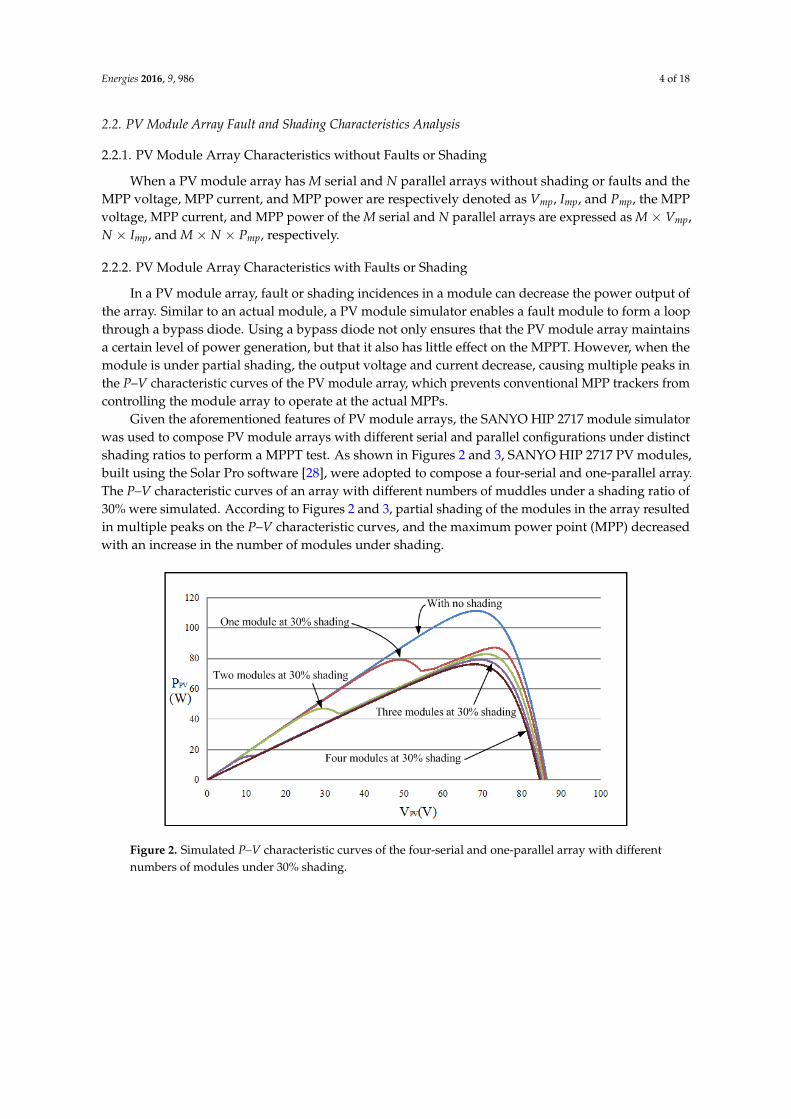
Given the aforementioned features of PV module arrays, the SANYO HIP 2717 module simulatorwas used to compose PV module arrays with different serial and parallel configurations under distinctshading ratios to perform a MPPT test. As shown in Figures 2 and 3, SANYO HIP 2717 PV modules,built using the Solar Pro software [28], were adopted to compose a four-serial and one-parallel array.The P–V characteristic curves of an array with different numbers of muddles under a shading ratio of30% were simulated. According to Figures 2 and 3, partial shading of the modules in the array resultedin multiple peaks on the P–V characteristic curves, and the maximum power point (MPP) decreasedwith an increase in the number of modules under shading.

Energies 2016, 9, 986 4 of 18

2.2. PV Module Array Fault and Shading Characteristics Analysis

2.2.1. PV Module Array Characteristics without Faults or Shading

When a PV module array has M serial and N parallel arrays without shading or faults and the

MPP voltage, MPP current, and MPP power are respectively denoted as Vmp, Imp, and Pmp, the MPP

voltage, MPP current, and MPP power of the M serial and N parallel arrays are expressed as M × Vmp,

N × Imp, and M × N × Pmp, respectively.

2.2.2. PV Module Array Characteristics with Faults or Shading

In a PV module array, fault or shading incidences in a module can decrease the power output of

the array. Similar to an actual module, a PV module simulator enables a fault module to form a loop

through a bypass diode. Using a bypass diode not only ensures that the PV module array maintains

a certain level of power generation, but that it also has little effect on the MPPT. However, when the

module is under partial shading, the output voltage and current decrease, causing multiple peaks in

the P–V characteristic curves of the PV module array, which prevents conventional MPP trackers

from controlling the module array to operate at the actual MPPs.

Given the aforementioned features of PV module arrays, the SANYO HIP 2717 module

simulator was used to compose PV module arrays with different serial and parallel configurations

under distinct shading ratios to perform a MPPT test. As shown in Figures 2 and 3, SANYO HIP 2717

PV modules, built using the Solar Pro software [28], were adopted to compose a four-serial and one-

parallel array. The P–V characteristic curves of an array with different numbers of muddles under a

shading ratio of 30% were simulated. According to Figures 2 and 3, partial shading of the modules in

the array resulted in multiple peaks on the P–V characteristic curves, and the maximum power point

(MPP) decreased with an increase in the number of modules under shading.

Figure 2. Simulated P–V characteristic curves of the four-serial and one-parallel array with different

numbers of modules under 30% shading.

Figure 2. Simulated P–V characteristic curves of the four-serial and one-parallel array with differentnumbers of modules under 30% shading.

Energies 2016, 9, 986 5 of 18Energies 2016, 9, 986 5 of 18

Figure 3. Simulated I–V characteristic curves of the four-serial and one-parallel array with different

numbers of modules under 30% shading.

3. Teaching-Learning-Based Optimization (TLBO) Method

TLBO was proposed by Rao, Savsani, and Vakharia [29] in 2011. The concept of TLBO is to

simulate the learning process between a teacher and students, the aim of which is to improve the

grades of the entire class through teacher instruction and mutual learning between students. The

students are comparable to individuals in an evolutionary algorithm and the teacher represents the

optimal individual according to the fitness values.

3.1. Conventional TLBO Method

The steps of the traditional TLBO algorithm are as follows:

Step 1: Set the values for the number of students Np, subjects m, and iterations E.

Step 2: Initialize a class S and define the following parameters:

(a) Random student: 1 2 3{ , , ,..., }Pk NX X X X X

(b) Random subject:1 2 3{ , , ,..., }j mX X X X X

(c) Target grade of student k in subject j:,j kG

Step 3: In the teaching phase, learning step ri, teaching factor TF, and students with the highest grades

Xj,k_best are given. The mean of a class is calculated according to Equation (3) and substituted

into Equation (4) to determine the student mean difference value. Finally, student grades are

updated according to Equation (5) to identify the new target grade for each student in the

teaching phase:

1

PN

k

k P

XM

N

(3)

, , __ ( ) 1,2,...,j k i j k best FDifferent Mean r X T M i E

(4)

, ( ) , ( ) ,_j k new j k old j kX X Different Mean

(5)

Step 4: In the learning phase, we assume that two random students XP and XQ participate in mutual

learning, in which the student with the lower grade learns from the one with a higher grade.

Adjustments were made using Equation (6):

Figure 3. Simulated I–V characteristic curves of the four-serial and one-parallel array with differentnumbers of modules under 30% shading.

3. Teaching-Learning-Based Optimization (TLBO) Method

TLBO was proposed by Rao, Savsani, and Vakharia [29] in 2011. The concept of TLBO is tosimulate the learning process between a teacher and students, the aim of which is to improve the gradesof the entire class through teacher instruction and mutual learning between students. The studentsare comparable to individuals in an evolutionary algorithm and the teacher represents the optimalindividual according to the fitness values.

3.1. Conventional TLBO Method

The steps of the traditional TLBO algorithm are as follows:

Step 1: Set the values for the number of students Np, subjects m, and iterations E.Step 2: Initialize a class S and define the following parameters:

(a) Random student: Xk ⊂{

X1, X2, X3, . . . , XNP

}(b) Random subject: Xj ⊂ {X1, X2, X3, . . . , Xm}(c) Target grade of student k in subject j: Gj,k

Step 3: In the teaching phase, learning step ri, teaching factor TF, and students with the highest gradesXj,k_best are given. The mean of a class is calculated according to Equation (3) and substitutedinto Equation (4) to determine the student mean difference value. Finally, student grades areupdated according to Equation (5) to identify the new target grade for each student in theteaching phase:

M =NP

∑k=1

XkNP

(3)

Di f f erent_Meanj,k = ri(Xj,k_best − TF ×M) i = 1, 2, . . . , E (4)

Xj,k(new) = Xj,k(old) + Di f f erent_Meanj,k (5)

Step 4: In the learning phase, we assume that two random students XP and XQ participate in mutuallearning, in which the student with the lower grade learns from the one with a higher grade.Adjustments were made using Equation (6):

Energies 2016, 9, 986 6 of 18

X′ j,k(new) = Xj,k(new) +

{ri(Xj,P(=k) − Xj,Q( 6=k)ri(Xj,Q(=k) − Xj,P( 6=k)

}, i f Xj,P > Xj,Q, i f Xj,Q > Xj,P

XP, XQ ⊂{

X1, X2, X3, . . . , XNP

} (6)

Step 5: Repeat steps 3 and 4 until the iteration is completed.

Parameters used in conventional TLBO are explained as follows:

Number of students (Np): Total number of participating students.Number of iterations (E): Number of teaching and learning phases that the students experience.Subject grade (Xj,k): Grade of student k in subject j. Five subjects were used in the present study.

Class mean (M): Mean grade of the class.Teaching step (ri): Parameter for diversifying the student mean difference with a random valuebetween 0 and 1.Teaching factor (TF): Teachers’ ability to teach the students. The parameter randomly generates a valueof 1 or 2.

In conventional TLBO, the teaching factors (TF) used in the teaching phase generally comprisetwo fixed teaching capabilities (1 or 2). However, in real teaching situations, students’ levels differand their learning capacity varies. Using fixed teaching factors may reduce learning effectiveness.In addition, learning from others (chosen at random) without conforming to students’ individuallearning levels might not optimize their learning effectiveness. Thus, this study proposes an improvedTLBO (I-TLBO) to solve the problems with conventional TLBO.

3.2. The Proposed I-TLBO Method

In the proposed I-TLBO, Steps 3 and 4 in conventional TLBO are modified through the followingthree improvements:

Modification 1: The teaching factors TF were modified to be automatically adjustable according to thestudents’ learning capacity. The adjustment method is expressed in Equation (7):

TF =Xj,k

Xj,k_best(7)

Modification 2: In the learning phase, a student selects another student who could benefit their learningthe most in order to boost their learning effectiveness.Modification 3: A self-study process was incorporated into the learning phase to enable each studentto adjust their self-learning according to their previous experience, as expressed in Equation (8):

X′′ j,k(new) = X′ j,k(new) + ri(X′ j,k(new) − X′ j,k−1(new)) i = 1, 2, . . . , E (8)

In Equation (4), if Xj,k_best and M remain unchanged, then Different_Meanj,k increases as TFdecreases. According to the actual MPPT process of PV module arrays, the tracking incrementis directly proportional to the distance between the individual student grades and the MPP. Therefore,if the student grades in Improvement 1 are X1 (i.e., power value P1) and X′1 (i.e., power value P′1),then the teaching factors TF of the student with the highest grades among all the students Xj,k_best (i.e.,MPP value tracked so far Pk_best) are modified using Equations (9) and (10):

TF1 =P1

Pk_best(9)

TF2 =P′1

Pk_best(10)

Energies 2016, 9, 986 7 of 18

As depicted in Figure 4, the TF1 value decreases as the Different_Mean value increases whenstudent grade is distant from the MPP (e.g., X1 position), thereby increasing the number of trackingsteps needed to approach the maximum value rapidly. By contrast, when the student grade is close tothe MPP (e.g., X′1 position), the TF2 value increases as the Different_Mean value and number of trackingsteps decrease to approach the maximum value slowly. Thus, the students can adjust their trackingsteps according to their learning capacity. In improvements 2 and 3, students can spontaneously learnfrom a student who is helpful to them. The term X′j,k-1(new) represents the student’s previous learningabilities, which is used as a basis for the other student’s self-study. In summary, the self-learningmethod not only accelerates the learning progress, but also escapes local solutions and reaches globalconvergence. A flowchart of the proposed I-TLBO MPPT is shown in Figure 5.

Energies 2016, 9, 986 7 of 18

12

_

'F

k best

PT

P

(10)

As depicted in Figure 4, the TF1 value decreases as the Different_Mean value increases when

student grade is distant from the MPP (e.g., X1 position), thereby increasing the number of tracking

steps needed to approach the maximum value rapidly. By contrast, when the student grade is close

to the MPP (e.g., X′1 position), the TF2 value increases as the Different_Mean value and number of

tracking steps decrease to approach the maximum value slowly. Thus, the students can adjust their

tracking steps according to their learning capacity. In improvements 2 and 3, students can

spontaneously learn from a student who is helpful to them. The term X′j,k-1(new) represents the student’s

previous learning abilities, which is used as a basis for the other student’s self-study. In summary,

the self-learning method not only accelerates the learning progress, but also escapes local solutions

and reaches global convergence. A flowchart of the proposed I-TLBO MPPT is shown in Figure 5.

Figure 4. Adjustment of teaching factors of the proposed I-TLBO.

3.3. MPP Tracker

Figure 6 depicts the MPP tracker architecture of the PV module array based on the proposed I-

TLBO. The architecture mainly comprises two subsystems: a DC/DC boost converter and I-TLBO-

based MPPT controller. When employed in a DC/DC boost converter, a synchronous rectification is

known to outperform a diode rectification in terms of the conversion efficiency as well as the thermal

performance [30], while a diode rectification is adopted instead in this work due to the reliability

concern. As stated previously, the I-TLBO-based MPPT controller controls the duty cycle of the boost

converter, enabling the PV module array to generate the maximum power output under partial

shading.

Table 2 lists the DC/DC boost converter parameter settings [31] and Table 3 lists the conventional

TLBO parameter settings. The component choices are made according to [31]. Without extra effort,

components available in our laboratories but with over specified ratings, are directly taken to

implement the DC/DC boost converter. In I-TLBO, the TF in Table 3 is replaced with the parameter

setting in Table 4 whereas all other parameters remain unchanged. Subsequently, the PV module

array was tested under five distinct operating situations, as shown in Table 5.

Figure 4. Adjustment of teaching factors of the proposed I-TLBO.

3.3. MPP Tracker

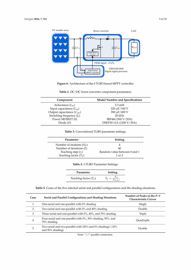
Figure 6 depicts the MPP tracker architecture of the PV module array based on the proposedI-TLBO. The architecture mainly comprises two subsystems: a DC/DC boost converter andI-TLBO-based MPPT controller. When employed in a DC/DC boost converter, a synchronousrectification is known to outperform a diode rectification in terms of the conversion efficiency aswell as the thermal performance [30], while a diode rectification is adopted instead in this work due tothe reliability concern. As stated previously, the I-TLBO-based MPPT controller controls the duty cycleof the boost converter, enabling the PV module array to generate the maximum power output underpartial shading.

Table 2 lists the DC/DC boost converter parameter settings [31] and Table 3 lists the conventionalTLBO parameter settings. The component choices are made according to [31]. Without extraeffort, components available in our laboratories but with over specified ratings, are directly taken toimplement the DC/DC boost converter. In I-TLBO, the TF in Table 3 is replaced with the parametersetting in Table 4 whereas all other parameters remain unchanged. Subsequently, the PV module arraywas tested under five distinct operating situations, as shown in Table 5.

Energies 2016, 9, 986 8 of 18Energies 2016, 9, 986 8 of 18

Start

Extract the PV module array output

voltage and current and calculate the

power output

1k k

Choose two students and with maximum

grade difference participate in mutual learning

P QX X

> ?P QX X

, ( ) , ( ) , ( ) , ( )( ) ' ij k new j k new j P k j Q kX X r X X

, ( ) , ( ) , ( ) , 1( )

Update the grades through the self-study formula

'' ' ( ' ' )j k new j k new i j k new j k newX X r X X

End

Output all students corresponding

duty cycle of the converter

Is the number

of iterations achieved?

Yes

No

No

No

Yes

Yes

Initialize relevant data

Student k=1

Setect the student with the optimal grade as Xk_best

Calculate

Different_Meanj,k=ri(Xj,k_best-TF×M)

, ( ) , ( ) ,

Update

_j k new j k old j kX X Different Mean

Have all students

Completed their learning

?

( ) ( ), ,, ( ) , ( ) ( ) ' Q k P ki j jj k new j k newX X r X X

Calculate corresponding

converter duty cycle and

output the value

,

Figure 5. MPPT flow chart of the proposed I-TLBO. Figure 5. MPPT flow chart of the proposed I-TLBO.

Energies 2016, 9, 986 9 of 18Energies 2016, 9, 986 9 of 18

Cin

DLm

CoutRLoad

Ipv

Vpv

PV module array Boost converter Load

PWM signal

TLBO-based

MPPT controller

TMS320F2808

Digital signal processor

S

Gate drive

circuit

Figure 6. Architecture of the I-TLBO-based MPPT controller.

Table 2. DC/DC boost converter component parameters.

Component Model Number and Specifications

Inductance (Lm) 3.3 mH

Input capacitance (Cin) 220 μF/160 V

Output capacitance (Cout) 390 μF/450 V

Switching frequency (fs) 20 kHz

Power MOSFET (S) IRF460 (500 V/20A)

Diode (D) DSEP30-12A (1200 V/30A)

Table 3. Conventional TLBO parameter settings.

Parameter Setting

Number of students (NP) 4

Number of iterations (E) 40

Teaching step (ri) Random value between 0 and 1

Teaching factor (TF) 1 or 2

Table 4. I-TLBO Parameter Settings.

Parameter Setting

Teaching factor (TF) ,

, _

j k

F

j k best

XT

X

Table 5. Cases of the five selected serial and parallel configurations and the shading situations.

Case Serial and Parallel Configurations and Shading Situations Number of Peaks in the P–V

Characteristic Curves

1 One-serial and one-parallel with 0% shading Single

2 Two-serial and one-parallel with 0% and 40% shading Double

3 Three-serial and one-parallel with 0%, 40%, and 70% shading Triple

4 Four-serial and one-parallel with 0%, 30% shading, 50%, and

70% shading Quadruple

5 Two-serial and two-parallel with (30% and 0% shading)//(0%

and 50% shading) Double

Note: “//” parallel connection.

Figure 6. Architecture of the I-TLBO-based MPPT controller.

Table 2. DC/DC boost converter component parameters.

Component Model Number and Specifications

Inductance (Lm) 3.3 mHInput capacitance (Cin) 220 µF/160 V

Output capacitance (Cout) 390 µF/450 VSwitching frequency (fs) 20 kHz

Power MOSFET (S) IRF460 (500 V/20A)Diode (D) DSEP30-12A (1200 V/30A)

Table 3. Conventional TLBO parameter settings.

Parameter Setting

Number of students (NP) 4Number of iterations (E) 40

Teaching step (ri) Random value between 0 and 1Teaching factor (TF) 1 or 2

Table 4. I-TLBO Parameter Settings.

Parameter Setting

Teaching factor (TF) TF =Xj,k

Xj,k_best

Table 5. Cases of the five selected serial and parallel configurations and the shading situations.

Case Serial and Parallel Configurations and Shading Situations Number of Peaks in the P–VCharacteristic Curves

1 One-serial and one-parallel with 0% shading Single

2 Two-serial and one-parallel with 0% and 40% shading Double

3 Three-serial and one-parallel with 0%, 40%, and 70% shading Triple

4 Four-serial and one-parallel with 0%, 30% shading, 50%, and70% shading Quadruple

5 Two-serial and two-parallel with (30% and 0% shading)//(0%and 50% shading) Double

Note: “//” parallel connection.

Energies 2016, 9, 986 10 of 18

4. Measurement Results

The PV module simulator circuit in Figure 1 was employed to compose the module arrayconfigurations under five operating situations as listed in Table 5. The P–V and I–V characteristiccurves of PV module arrays under different shading ratios were measured using an MP 170 I–Vchecker by EKO Instruments CO. Ltd (Tokyo, Japan). The aim is to tell whether the global MPPs in the5 testing cases listed in Table 5 can be tracked as expected using I-TBLO MPPT. Subsequently, a digitalsignal processor TMS320F2808 [32] was used to perform MPPT by using conventional TLBO and theproposed I-TLBO. The tracking performance of the two methods was also compared.

4.1. PV Module Array Characteristics under Different Operating Situations

Figures 7–11 depict the I–V and P–V characteristic curves of the PV module arrays under the fiveoperating situations listed in Table 5. Figure 7 shows the output characteristics of a single PV module.The output characteristic curve reveals that the parameters related to the output characteristics ofmodules not affected by shading or faults are identical to the electricity parameter specificationslisted in Table 1. The module in Figure 7 was used as a basis for testing the serial configurations (i.e.,Cases 1–4) as well as the serial and parallel configurations (Case 5), as listed in Table 5. Different shadingratio conditions were set to produce multiple peaks in the characteristic curves to exemplify theexceptional performance of the proposed I-TLBO on MPPT. Figures 8–10 reveal that double, triple,and quadruple peaks occur in Cases 2 to 4. Thus, we inferred that N peaks would appear in P–Vcharacteristic curves when N modules in a serial array were under different shading ratios. Figure 11shows the I–V and P–V characteristic curves measured on the two-serial and two-parallel configurationmodule array of Case 5. Although two modules in each serial module were subjected to differentshading ratios, the parallel connection between the two-serial modules generated double peaks only inthe P–V characteristic curve.

Energies 2016, 9, 986 10 of 18

4. Measurement Results

The PV module simulator circuit in Figure 1 was employed to compose the module array

configurations under five operating situations as listed in Table 5. The P–V and I–V characteristic

curves of PV module arrays under different shading ratios were measured using an MP 170 I–V

checker by EKO Instruments CO. Ltd (Tokyo, Japan). The aim is to tell whether the global MPPs in

the 5 testing cases listed in Table 5 can be tracked as expected using I-TBLO MPPT. Subsequently, a

digital signal processor TMS320F2808 [32] was used to perform MPPT by using conventional TLBO

and the proposed I-TLBO. The tracking performance of the two methods was also compared.

4.1. PV Module Array Characteristics under Different Operating Situations

Figures 7–11 depict the I–V and P–V characteristic curves of the PV module arrays under the five

operating situations listed in Table 5. Figure 7 shows the output characteristics of a single PV module.

The output characteristic curve reveals that the parameters related to the output characteristics of

modules not affected by shading or faults are identical to the electricity parameter specifications listed

in Table 1. The module in Figure 7 was used as a basis for testing the serial configurations (i.e., Cases

1–4) as well as the serial and parallel configurations (Case 5), as listed in Table 5. Different shading

ratio conditions were set to produce multiple peaks in the characteristic curves to exemplify the

exceptional performance of the proposed I-TLBO on MPPT. Figures 8–10 reveal that double, triple,

and quadruple peaks occur in Cases 2 to 4. Thus, we inferred that N peaks would appear in P–V

characteristic curves when N modules in a serial array were under different shading ratios. Figure 11

shows the I–V and P–V characteristic curves measured on the two-serial and two-parallel

configuration module array of Case 5. Although two modules in each serial module were subjected

to different shading ratios, the parallel connection between the two-serial modules generated double

peaks only in the P–V characteristic curve.

Figure 7. I–V and P–V characteristic curves of one-serial and one-parallel module array with 0%

shading.

0

0.2

0.4

0.6

0.8

1

1.2

1.4

1.6

1.8

2

0

5

10

15

20

25

30

0 5 10 15 20 25

VPV(V)

IPV

(A)

PPV

(W)

I-V curve

P-V curve

Pmax=27.8W

Figure 7. I–V and P–V characteristic curves of one-serial and one-parallel module array with0% shading.

Energies 2016, 9, 986 11 of 18Energies 2016, 9, 986 11 of 18

Figure 8. I–V and P–V characteristic curves of the two-serial and one-parallel module array with 0%

and 40% shading.

Figure 9. I–V and P–V characteristic curves of the three-serial and one-parallel module array with 0%,

30%, and 70% shading.

Figure 10. I–V and P–V characteristic curves of the four-serial and one-parallel module array with 0%,

30%, 50%, and 70% shading.

Figure 8. I–V and P–V characteristic curves of the two-serial and one-parallel module array with 0%and 40% shading.

Energies 2016, 9, 986 11 of 18

Figure 8. I–V and P–V characteristic curves of the two-serial and one-parallel module array with 0%

and 40% shading.

Figure 9. I–V and P–V characteristic curves of the three-serial and one-parallel module array with 0%,

30%, and 70% shading.

Figure 10. I–V and P–V characteristic curves of the four-serial and one-parallel module array with 0%,

30%, 50%, and 70% shading.

Figure 9. I–V and P–V characteristic curves of the three-serial and one-parallel module array with 0%,30%, and 70% shading.

Energies 2016, 9, 986 11 of 18

Figure 8. I–V and P–V characteristic curves of the two-serial and one-parallel module array with 0%

and 40% shading.

Figure 9. I–V and P–V characteristic curves of the three-serial and one-parallel module array with 0%,

30%, and 70% shading.

Figure 10. I–V and P–V characteristic curves of the four-serial and one-parallel module array with 0%,

30%, 50%, and 70% shading.

Figure 10. I–V and P–V characteristic curves of the four-serial and one-parallel module array with 0%,30%, 50%, and 70% shading.

Energies 2016, 9, 986 12 of 18Energies 2016, 9, 986 12 of 18

Figure 11. I–V and P–V characteristic curves of the two-serial and two-parallel module array with

[(0% and 30% shading)//(0% and 50% shading)].

4.2. MPPT Measurement of PV Module Arrays

The measurement architecture is shown in Figure 6. First, the output voltage VPV and current IPV

of the PV module arrays were extracted through sensors and signal conversion circuits and entered

into the TMS320F2808 digital signal processor. Subsequently, TLBO was applied to perform MPPT.

The resulting optimal duty cycle trigger signal was sent to the boost converter to control the on time

of power transistors, thereby controlling the maximum power output of the PV module array.

Figures 12–16 show the waveforms of output voltage VPV and current IPV measured on the PV

module arrays. The power curves are demonstrated as the product of voltage and current through

the internal computation functions of the oscilloscope. In the 40th iteration, the quality of the

conventional TLBO and the proposed I-TLBO tracking response speed were observed and compared

when the power curve approached a stable value.

4.2.1. Case 1 (One-Serial and One-Parallel: 0% Shading)

Figure 12a,b depict the MPPT waveforms of Case 1 (0% shading) measured by using the

conventional TLBO and the proposed I-TLBO, respectively. The results revealed that under standard

test conditions, the output characteristics of the PV module simulator were identical to the electricity

parameter specifications in Table 1. In addition, the tracking time between time points t0 and t1 in

Figure 12 showed that the proposed I-TLBO (2.5 s) converged faster than did conventional TLBO (3.5 s).

(a)

Figure 11. I–V and P–V characteristic curves of the two-serial and two-parallel module array with[(0% and 30% shading)//(0% and 50% shading)].

4.2. MPPT Measurement of PV Module Arrays

The measurement architecture is shown in Figure 6. First, the output voltage VPV and current IPVof the PV module arrays were extracted through sensors and signal conversion circuits and enteredinto the TMS320F2808 digital signal processor. Subsequently, TLBO was applied to perform MPPT.The resulting optimal duty cycle trigger signal was sent to the boost converter to control the on time ofpower transistors, thereby controlling the maximum power output of the PV module array.

Figures 12–16 show the waveforms of output voltage VPV and current IPV measured on the PVmodule arrays. The power curves are demonstrated as the product of voltage and current through theinternal computation functions of the oscilloscope. In the 40th iteration, the quality of the conventionalTLBO and the proposed I-TLBO tracking response speed were observed and compared when thepower curve approached a stable value.

4.2.1. Case 1 (One-Serial and One-Parallel: 0% Shading)

Figure 12a,b depict the MPPT waveforms of Case 1 (0% shading) measured by using theconventional TLBO and the proposed I-TLBO, respectively. The results revealed that under standardtest conditions, the output characteristics of the PV module simulator were identical to the electricityparameter specifications in Table 1. In addition, the tracking time between time points t0 and t1 inFigure 12 showed that the proposed I-TLBO (2.5 s) converged faster than did conventional TLBO (3.5 s).

Energies 2016, 9, 986 12 of 18

Figure 11. I–V and P–V characteristic curves of the two-serial and two-parallel module array with

[(0% and 30% shading)//(0% and 50% shading)].

4.2. MPPT Measurement of PV Module Arrays

The measurement architecture is shown in Figure 6. First, the output voltage VPV and current IPV

of the PV module arrays were extracted through sensors and signal conversion circuits and entered

into the TMS320F2808 digital signal processor. Subsequently, TLBO was applied to perform MPPT.

The resulting optimal duty cycle trigger signal was sent to the boost converter to control the on time

of power transistors, thereby controlling the maximum power output of the PV module array.

Figures 12–16 show the waveforms of output voltage VPV and current IPV measured on the PV

module arrays. The power curves are demonstrated as the product of voltage and current through

the internal computation functions of the oscilloscope. In the 40th iteration, the quality of the

conventional TLBO and the proposed I-TLBO tracking response speed were observed and compared

when the power curve approached a stable value.

4.2.1. Case 1 (One-Serial and One-Parallel: 0% Shading)

Figure 12a,b depict the MPPT waveforms of Case 1 (0% shading) measured by using the

conventional TLBO and the proposed I-TLBO, respectively. The results revealed that under standard

test conditions, the output characteristics of the PV module simulator were identical to the electricity

parameter specifications in Table 1. In addition, the tracking time between time points t0 and t1 in

Figure 12 showed that the proposed I-TLBO (2.5 s) converged faster than did conventional TLBO (3.5 s).

(a)

Figure 12. Cont.

Energies 2016, 9, 986 13 of 18Energies 2016, 9, 986 13 of 18

(b)

Figure 12. Measurement results of the one-serial and one-parallel module array with 0% shading by

using (a) conventional TLBO (Pmp = 27.4 W) and (b) the proposed I-TLBO (Pmp = 27.8 W).

4.2.2. Case 2 (Two-Serial and One-Parallel: 0% and 40% Shading)

Figure 13a,b depict the MPPT waveforms of Case 2 measured by using conventional TLBO and

the proposed I-TLBO, respectively. The two-serial and one-parallel configuration was composed on

the basis of the single module of Case 1. One module in Case 2 was under 40% shading. The empirical

results revealed that under partial shading, the PV module array generated a double-peaked P–V

characteristic curve (Figure 8). Although both the conventional and proposed methods tracked the

actual MPP, the proposed I-TLBO (2.4 s) was faster than conventional TLBO (2.7 s) in MPPT response

speed.

(a)

Figure 12. Measurement results of the one-serial and one-parallel module array with 0% shading byusing (a) conventional TLBO (Pmp = 27.4 W) and (b) the proposed I-TLBO (Pmp = 27.8 W).

4.2.2. Case 2 (Two-Serial and One-Parallel: 0% and 40% Shading)

Figure 13a,b depict the MPPT waveforms of Case 2 measured by using conventional TLBO andthe proposed I-TLBO, respectively. The two-serial and one-parallel configuration was composed onthe basis of the single module of Case 1. One module in Case 2 was under 40% shading. The empiricalresults revealed that under partial shading, the PV module array generated a double-peaked P–Vcharacteristic curve (Figure 8). Although both the conventional and proposed methods trackedthe actual MPP, the proposed I-TLBO (2.4 s) was faster than conventional TLBO (2.7 s) in MPPTresponse speed.

Energies 2016, 9, 986 13 of 18

(b)

Figure 12. Measurement results of the one-serial and one-parallel module array with 0% shading by

using (a) conventional TLBO (Pmp = 27.4 W) and (b) the proposed I-TLBO (Pmp = 27.8 W).

4.2.2. Case 2 (Two-Serial and One-Parallel: 0% and 40% Shading)

Figure 13a,b depict the MPPT waveforms of Case 2 measured by using conventional TLBO and

the proposed I-TLBO, respectively. The two-serial and one-parallel configuration was composed on

the basis of the single module of Case 1. One module in Case 2 was under 40% shading. The empirical

results revealed that under partial shading, the PV module array generated a double-peaked P–V

characteristic curve (Figure 8). Although both the conventional and proposed methods tracked the

actual MPP, the proposed I-TLBO (2.4 s) was faster than conventional TLBO (2.7 s) in MPPT response

speed.

(a)

Figure 13. Cont.

Energies 2016, 9, 986 14 of 18Energies 2016, 9, 986 14 of 18

(b)

Figure 13. Measurement results of the two-serial and one-parallel module array (0% and 40% shading)

by using (a) conventional TLBO (Pmp = 35.1 W) and (b) the proposed I-TLBO (Pmp = 35.8 W).

4.2.3. Case 3 (Three-Serial and One-Parallel: 0%, 30%, and 70% Shading)

Figure 14a,b depict the MPPT waveforms Case 3 measured by using conventional TLBO and the

proposed I-TLBO, respectively. The empirical results revealed that three modules under different

shading ratios generated triple peaks in the P–V characteristic curve and a long tracking time under

conventional TLBO (3.4 s). By contrast, the proposed I-TLBO (2.7 s) tracked the real MPPT in less time.

(a)

(b)

Figure 14. Measurement results of the three-serial and one-parallel module array (0%, 30%, and 70%

shading) by using (a) conventional TLBO (Pmp = 37.7 W) and (b) the proposed I-TLBO (Pmp = 38.5 W).

Figure 13. Measurement results of the two-serial and one-parallel module array (0% and 40% shading)by using (a) conventional TLBO (Pmp = 35.1 W) and (b) the proposed I-TLBO (Pmp = 35.8 W).

4.2.3. Case 3 (Three-Serial and One-Parallel: 0%, 30%, and 70% Shading)

Figure 14a,b depict the MPPT waveforms Case 3 measured by using conventional TLBO andthe proposed I-TLBO, respectively. The empirical results revealed that three modules under differentshading ratios generated triple peaks in the P–V characteristic curve and a long tracking time underconventional TLBO (3.4 s). By contrast, the proposed I-TLBO (2.7 s) tracked the real MPPT in less time.

Energies 2016, 9, 986 14 of 18

(b)

Figure 13. Measurement results of the two-serial and one-parallel module array (0% and 40% shading)

by using (a) conventional TLBO (Pmp = 35.1 W) and (b) the proposed I-TLBO (Pmp = 35.8 W).

4.2.3. Case 3 (Three-Serial and One-Parallel: 0%, 30%, and 70% Shading)

Figure 14a,b depict the MPPT waveforms Case 3 measured by using conventional TLBO and the

proposed I-TLBO, respectively. The empirical results revealed that three modules under different

shading ratios generated triple peaks in the P–V characteristic curve and a long tracking time under

conventional TLBO (3.4 s). By contrast, the proposed I-TLBO (2.7 s) tracked the real MPPT in less time.

(a)

(b)

Figure 14. Measurement results of the three-serial and one-parallel module array (0%, 30%, and 70%

shading) by using (a) conventional TLBO (Pmp = 37.7 W) and (b) the proposed I-TLBO (Pmp = 38.5 W). Figure 14. Measurement results of the three-serial and one-parallel module array (0%, 30%, and 70%shading) by using (a) conventional TLBO (Pmp = 37.7 W) and (b) the proposed I-TLBO (Pmp = 38.5 W).

Energies 2016, 9, 986 15 of 18

4.2.4. Case 4 (Four-Serial and One-Parallel: 0%, 30%, 50%, and 70% Shading)

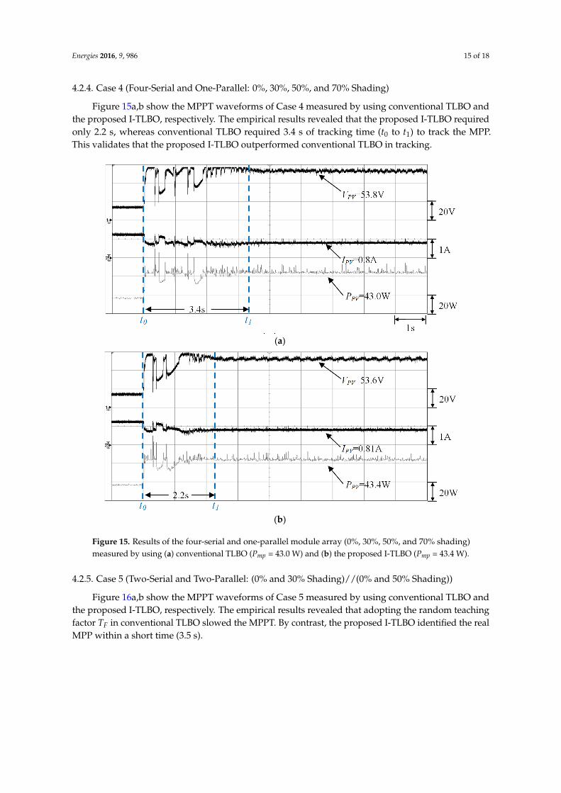
Figure 15a,b show the MPPT waveforms of Case 4 measured by using conventional TLBO andthe proposed I-TLBO, respectively. The empirical results revealed that the proposed I-TLBO requiredonly 2.2 s, whereas conventional TLBO required 3.4 s of tracking time (t0 to t1) to track the MPP.This validates that the proposed I-TLBO outperformed conventional TLBO in tracking.

Energies 2016, 9, 986 15 of 18

4.2.4. Case 4 (Four-Serial and One-Parallel: 0%, 30%, 50%, and 70% Shading)

Figure 15a,b show the MPPT waveforms of Case 4 measured by using conventional TLBO and

the proposed I-TLBO, respectively. The empirical results revealed that the proposed I-TLBO required

only 2.2 s, whereas conventional TLBO required 3.4 s of tracking time (t0 to t1) to track the MPP. This

validates that the proposed I-TLBO outperformed conventional TLBO in tracking.

(a)

(b)

Figure 15. Results of the four-serial and one-parallel module array (0%, 30%, 50%, and 70% shading)

measured by using (a) conventional TLBO (Pmp = 43.0 W) and (b) the proposed I-TLBO (Pmp = 43.4 W).

4.2.5. Case 5 (Two-Serial and Two-Parallel: (0% and 30% Shading)//(0% and 50% Shading))

Figure 16a,b show the MPPT waveforms of Case 5 measured by using conventional TLBO and

the proposed I-TLBO, respectively. The empirical results revealed that adopting the random teaching

factor TF in conventional TLBO slowed the MPPT. By contrast, the proposed I-TLBO identified the

real MPP within a short time (3.5 s).

Figure 15. Results of the four-serial and one-parallel module array (0%, 30%, 50%, and 70% shading)measured by using (a) conventional TLBO (Pmp = 43.0 W) and (b) the proposed I-TLBO (Pmp = 43.4 W).

4.2.5. Case 5 (Two-Serial and Two-Parallel: (0% and 30% Shading)//(0% and 50% Shading))

Figure 16a,b show the MPPT waveforms of Case 5 measured by using conventional TLBO andthe proposed I-TLBO, respectively. The empirical results revealed that adopting the random teachingfactor TF in conventional TLBO slowed the MPPT. By contrast, the proposed I-TLBO identified the realMPP within a short time (3.5 s).

Energies 2016, 9, 986 16 of 18Energies 2016, 9, 986 16 of 18

(a)

(b)

Figure 16. Results of the two-serial and two-parallel module array [(0% and 30% shading)//(0% and

50% shading)] measured by using (a) conventional TLBO (Pmp = 66.5 W) and (b) the proposed I-TLBO

(Pmp = 66.7 W).

4.2.6. Comparison of the Case Measurements

Table 6 gives the performance comparison in terms of the average tracking time and the average

MPP for 40 iterations among the proposed I-TBLO, a typical TLBO, ACO [17] and PSO [21], both

referred to in the Introduction section. This proposal is obviously found to outperform the

counterparts in terms of dynamic tracking response and static performance for the five cases

investigated in the present study underwent MPPT.

Table 6. Comparison between the measurement results of the five cases obtained using ACO, PSO,

conventional TLBO and the proposed I-TLBO.

Case P–V Curve

Peaks

ACO [17] PSO [21] Conventional TLBO Proposed I-TLBO

Average

Tracking

Time

Average

MPP

Average

Tracking

Time

Average

MPP

Average

Tracking

Time

Average

MPP

Average

Tracking

Time

Average

MPP

1 Single 4.3 s 27.5 W 3.4 s 27.3 W 3.3 s 27.0 W 2.5 s 27.8 W

2 Double 4.8 s 35.3 W 3.0 s 35.0 W 2.8 s 35.1 W 2.4 s 35.8 W

3 Triple 5.1 s 37.5 W 3.8 s 37.0 W 3.4 s 37.2 W 2.7 s 38.5 W

4 Quadrupe 5.6 s 43.2 W Tracking

failed 35.7 W 3.6 s 43.0 W 2.2 s 43.4 W

5 Double 5.8 s 66.3 W 5.2 s 64.7 W 4.8 s 66.1 W 3.7 s 66.7 W

Figure 16. Results of the two-serial and two-parallel module array [(0% and 30% shading)//(0% and50% shading)] measured by using (a) conventional TLBO (Pmp = 66.5 W) and (b) the proposed I-TLBO(Pmp = 66.7 W).

4.2.6. Comparison of the Case Measurements

Table 6 gives the performance comparison in terms of the average tracking time and the averageMPP for 40 iterations among the proposed I-TBLO, a typical TLBO, ACO [17] and PSO [21], bothreferred to in the Introduction section. This proposal is obviously found to outperform the counterpartsin terms of dynamic tracking response and static performance for the five cases investigated in thepresent study underwent MPPT.

Table 6. Comparison between the measurement results of the five cases obtained using ACO, PSO,conventional TLBO and the proposed I-TLBO.

Case P–V CurvePeaks

ACO [17] PSO [21] Conventional TLBO Proposed I-TLBO

AverageTracking

Time

AverageMPP

AverageTracking

Time

AverageMPP

AverageTracking

Time

AverageMPP

AverageTracking

Time

AverageMPP

1 Single 4.3 s 27.5 W 3.4 s 27.3 W 3.3 s 27.0 W 2.5 s 27.8 W2 Double 4.8 s 35.3 W 3.0 s 35.0 W 2.8 s 35.1 W 2.4 s 35.8 W3 Triple 5.1 s 37.5 W 3.8 s 37.0 W 3.4 s 37.2 W 2.7 s 38.5 W

4 Quadrupe 5.6 s 43.2 W Trackingfailed 35.7 W 3.6 s 43.0 W 2.2 s 43.4 W

5 Double 5.8 s 66.3 W 5.2 s 64.7 W 4.8 s 66.1 W 3.7 s 66.7 W

Energies 2016, 9, 986 17 of 18

5. Conclusions

In this study, an I-TLBO was proposed to perform MPPT of PV module arrays. To enhance theTLBO tracking efficiency and performance, an intellectual teaching factor adjustment method wasadopted to facilitate automatic adjustments of TLBO teaching factors. In addition, in the learningphase, the students automatically tracked the targets benefiting their learning. Eventually, eachstudent expedited their tracking speed through self-study according to their individual experience.The empirical results verified that the proposed I-TLBO can more rapidly identify the real MPPcompared with conventional TLBO, ACO and PSO when certain modules in a PV module array areunder partial shading. The results of the measurements of the designed five cases of shading confirmedthat the proposed I-TLBO tracked the global MPP within a shorter period than conventional TLBO,ACO and PSO can. These results confirm the feasibility of applying the proposed I-TLBO in PV modulearray MPPT, particularly in situations where multiple peaks occur on the P–V characteristic curvesbecause of partial shading. This proposed high performance tracking algorithm can be also directlyapplied to track the MPP for each single PV module using a DC/DC converter, and to track the MPPon a one-peak P–V curve using a central inverter.

Acknowledgments: The authors gratefully acknowledge the support of the Ministry of Science and Technology,Taiwan, Republic of China, under the Grant Number MOST 105-ET-E-167-001-ET.

Author Contributions: The improved teaching-learning-based optimization (I-TLBO) algorithm was proposed byKuei-Hsiang Chao, who was responsible for writing the paper. Meng-Cheng Wu carried out the simulations andexperiments concerning the typical and improved I-TLBO algorithm for photovoltaic power generation systems,meanwhile, comparing the dynamic tracking and steady-state performance of these two algorithms.

Conflicts of Interest: The authors declare no conflict of interest.

References

1. Wang, X.; Liang, H. Output characteristics of PV array under different insolation and temperature.In Proceedings of the IEEE 2012 Conference on Asia Pacific Power and Energy Engineering (APPEE),Shanghai, China, 27–29 March 2012; pp. 1–4.

2. Femia, N.; Granozio, D.; Petrone, G.; Spagnuolo, G.; Vitelli, M. Predictive and adaptive MPPT perturb andobserve method. IEEE Trans. Aerosp. Electron. Syst. 2007, 43, 934–950. [CrossRef]

3. Luigi, P.; Renato, R.; Ivan, S.; Pietro, T. Optimized adaptive perturb and observe maximum power pointtracking control for photovoltaic generation. Energies 2015, 8, 3418–3436. [CrossRef]

4. D’Souza, N.S.; Lopes, L.A.C.; Liu, X. Comparative study of variable size perturbation and observationmaximum power point trackers for PV systems. Electr. Power Syst. Res. 2010, 80, 296–305. [CrossRef]

5. Lin, C.H.; Huang, C.H.; Du, Y.C.; Chen, J.L. Maximum photovoltaic power tracking for the PV array usingthe fractional-order incremental conductance method. Appl. Energy 2011, 88, 4840–4847. [CrossRef]

6. Li, C.; Chen, Y.; Zhou, D.; Liu, J.; Zeng, J. A high-performance adaptive incremental conductance MPPTalgorithm for photovoltaic systems. Energies 2016, 9, 288–305. [CrossRef]

7. Mohammadmehdi, S.; Saad, M.; Rasoul, R.; Rubiyah, Y.; Ehsan, T.R. Analytical modeling of partially shadedphotovoltaic systems. Energies 2013, 6, 128–144. [CrossRef]

8. Balato, M.; Vitelli, M.; Femia, N.; Petrone, G.; Spagnuolo, G. Factors limiting the efficiency of DMPPT inPV applications. In Proceedings of the International Conference on Clean Electrical Power, Ischia, Italy,14–16 June 2011; pp. 604–608.

9. Vitelli, M. On the necessity of joint adoption of both distributed maximum power point tracking and centralmaximum power point tracking in PV systems. Prog. Photovolt. Res. Appl. 2014, 22, 283–299. [CrossRef]

10. Iacca, G.; Mallipeddi, R.; Mininno, E.; Neri, F.; Suganthan, P.N. Global supervision for compact differentialevolution. In Proceedings of the 2011 IEEE Symposium on Differential Evolution (SDE), Paris, France,11–15 April 2011; pp. 1–8.

11. Dorigo, M.; Birattari, M.; Stutzle, T. Ant colony optimization. IEEE Comput. Intell. Mag. 2006, 1, 28–39. [CrossRef]12. Gao, W.; Liu, S.; Huang, L. A global best artificial bee colony algorithm for global optimization. J. Comput.

Appl. Math. 2012, 236, 2741–2753. [CrossRef]

Energies 2016, 9, 986 18 of 18

13. Hadji, S.; Gaubert, J.P.; Krim, F. Genetic algorithms for maximum power point tracking in photovoltaicsystems. In Proceedings of the IEEE 2011—14th European Conference on Power Electronics and Applications(EPE), Birmingham, UK, 30 August–1 September 2011; pp. 1–9.

14. Hadji, S.; Gaubert, J.P.; Krim, F. Experimental analysis of genetic algorithms based MPPT for PV systems.In Proceedings of the IEEE Conference on International Renewable and Sustainable Energy (IRSEC),Ouarzazate, Morocco, 17–19 October 2014; pp. 7–12.

15. Tajuddin, M.F.N.; Ayob, S.M.; Salam, Z. Tracking of maximum power point in partial shading conditionusing differential evolution (DE). In Proceedings of the IEEE 2012 International Conference on Power andEnergy (PECon), Kota Kinabalu, Malaysia, 2–5 December 2012; pp. 384–389.

16. Storn, R. On the usage of differential evolution for function optimization. In Proceedings of the BiennialConference of the North American in Fuzzy Information Processing Society (NAFIPS), Berkeley, CA, USA,19–22 June1996; pp. 519–523.

17. Lian, J.; Maskell, D.L. A uniform implementation scheme for evolutionary optimization algorithms and theexperimental implementation of an ACO based MPPT for PV systems under partial shading. In Proceedingsof the IEEE Symposium on Computational Intelligence Applications in Smart Grid (CIASG), Orlando, FL,USA, 9–12 December 2014; pp. 1–8.

18. Sundareswaran, K.; Sankar, P.; Nayak, P.S.R.; Simon, S.P.; Palani, S. Enhanced energy output from a PVsystem under partial shaded conditions through artificial bee colony. IEEE Trans. Energy Convers. 2015, 6,198–209. [CrossRef]

19. Lian, K.L.; Jhang, J.H.; Tian, I.S. A maximum power point tracking method based on perturb-and-observecombined with particle swarm optimization. IEEE J. Photovolt. 2014, 4, 626–633. [CrossRef]

20. Daraban, S.; Petreus, D.; Morel, C. A novel global MPPT based on genetic algorithms for photovoltaicsystems under the influence of partial shading. In Proceedings of the IEEE 2013—39th Annual Conferenceon Industrial Electronics Society (IECON), Vienna, Austria, 10–13 November 2013; pp. 1490–1495.

21. Kashif, I.; Zainal, S.; Amir, S.; Muhammad, A. A direct control based maximum power point tracking methodfor photovoltaic system under partial shading conditions using particle swarm optimization algorithm.Appl. Energy 2012, 99, 414–422. [CrossRef]

22. Chao, K.H.; Lin, Y.S.; Lai, U.D. Improved particle swarm optimization for maximum power point tracking inphotovoltaic module arrays. Appl. Energy 2015, 158, 609–618. [CrossRef]

23. Rao, R.V.; Savsani, V.J.; Vakharia, D.P. Teaching-learning-based optimization: A novel method for constrainedmechanical design optimization problems. J. Comput. Aided Des. 2011, 43, 303–315. [CrossRef]

24. Satapathy, S.C.; Naik, A.; Parvathi, K. Weighted teaching-learning-based optimization for global functionoptimization. Appl. Math. Sci. Res. Publ. 2013, 4, 429–439. [CrossRef]

25. Rao, R.V.; Patel, V. An improved teaching-learning-based optimization Algorithm for solving unconstrainedoptimization problems. Comput. Sci. Eng. Electr. Eng. 2013, 20, 710–720. [CrossRef]

26. SANYO HIP 2717 Datasheet. Available online: http://iris.nyit.edu/~mbertome/solardecathlon/SDClerical/SD_DESIGN+DEVELOPMENT/091804_Sanyo190HITBrochure.pdf (accessed on 15 January 2016).

27. Chao, K.H.; Chao, Y.W.; Chen, J.P. A circuit-based photovoltaic module simulator with shadow andfault setting. Int. J. Electron. 2016, 103, 424–438. [CrossRef]

28. Solar Pro Official Website. Available online: http://lapsys.co.jp/english (accessed on 10 May 2016).29. Rao, R.V.; Patel, V.; Chen, J.P. An elitist teaching-learning-based optimization algorithm for solving complex

constrained optimization problems. Int. J. Ind. Eng. Comput. 2012, 3, 535–560. [CrossRef]30. Graditi, G.; Adinolfi, G.; Femia, N.; Vitelli, M. Comparative analysis of synchronous rectification boost and

diode rectification boost converter for DMPPT applications. In Proceedings of the 2011 IEEE InternationalSymposium on Industrial Electronics (ISIE), Gdansk, Poland, 27–30 June 2011; pp. 1000–1005.

31. Hart, D.W. Introduction to Power Electronics; Prentice Hall: New York, NY, USA, 2003.32. TMS320F2808 Data Sheet. Available online: http://www.ti.com/lit/ds/symlink/tms320f2808.pdf (accessed

on 12 March 2016).

© 2016 by the authors; licensee MDPI, Basel, Switzerland. This article is an open accessarticle distributed under the terms and conditions of the Creative Commons Attribution(CC-BY) license (http://creativecommons.org/licenses/by/4.0/).