global land use change and greenhouse gas emissions … · global land use change and greenhouse...

1

Global land use change and greenhouse gas emissions due to recent

European biofuel policies

Neus Escobara, Badri Narayananb, Wallace E. Tynerb

a Food Technology Department, Universitat Politècnica de València, Spain b Department of Agricultural Economics, Purdue University, IN United States

Abstract:

The European Union (EU) has emerged as a major producer and consumer of biodiesel, due to policy

initiatives. Recent policies seek to curb imports from USA, Argentina and Indonesia by imposing anti-

dumping duties. Further, there has been a proposal to set a cap on First Generation Biofuels (FGBs) to

reduce greenhouse gas (GHG) emissions from Land Use Change (LUC). In this paper, we employ the

widely used GTAP-BIO model to examine these recent EU policies. Increased biodiesel consumption

arising from the cap on FGBs and increased import prices arising from anti-dumping measures are both

modeled as exogenous policy shocks. We find that the biodiesel imports increase despite these anti-

dumping measures, because of the enormous expansion of domestic demand, mainly for palm biodiesel.

Biodiesel producers in the EU benefit from these policies as well, especially those producing rapeseed

and non-food-based biodiesel, but also palm biodiesel due to imports of vegetable oils. LUC is expected

to occur at a global scale as a consequence of biodiesel trade and interactions in the food and feed

markets. Besides the EU, other countries such as the US, Brazil or South-Saharan Africa can be affected.

1. Introduction

Biofuels production has been growing sharply all around the world during the last decade, as a

consequence of rising prices of oil together with the approval of public policies to mitigate the effects of

global warming. Most of these policies, such as the European Directive 2009/28/CE, aim at reducing the

greenhouse gas (GHG) emissions while increasing energy independence by introducing a blending

mandate. Specifically, this Directive (also known as the Renewable Energy Directive –RED-), establishes a

10% biofuel share in the motor fuel market of the Member States by 2020, while setting out a

sustainability criteria that requires biofuels to emit at least 35% less GHG than the replaced fossil fuel.

Biofuel emissions must be calculated over the entire life cycle and must include the corresponding losses

in carbon stocks if land has been converted to biofuel production. This is to ensure that increasing

biofuels consumption does not take place at the expense of carbon-rich ecosystems.

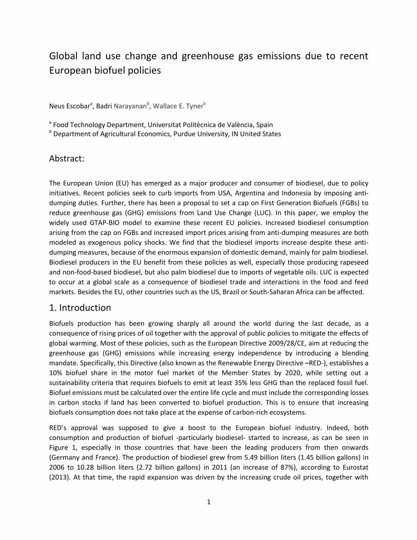
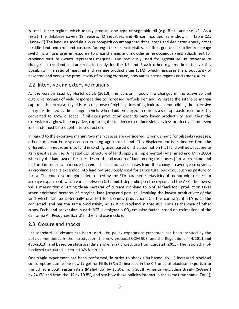
RED’s approval was supposed to give a boost to the European biofuel industry. Indeed, both

consumption and production of biofuel -particularly biodiesel- started to increase, as can be seen in

Figure 1, especially in those countries that have been the leading producers from then onwards

(Germany and France). The production of biodiesel grew from 5.49 billion liters (1.45 billion gallons) in

2006 to 10.28 billion liters (2.72 billion gallons) in 2011 (an increase of 87%), according to Eurostat

(2013). At that time, the rapid expansion was driven by the increasing crude oil prices, together with

2

subsidies on the production of oilseeds under Common Agricultural Policy set-aside programs (Flach et

al., 2013). Generous tax incentives on biodiesel production –mainly in Germany and France– also played

a great role, especially for the sector’s development. However, direct payments to farmers have been

progressively reduced (decoupling subsidies from particular crops since the 2003 reform), and tax

exemptions have been substantially reduced in most of the Member States due to the cost for the public

budget.

Figure 1. Data and projections for fuel and biofuel consumption in the European transport sector (EU27). Source: Eurostat.

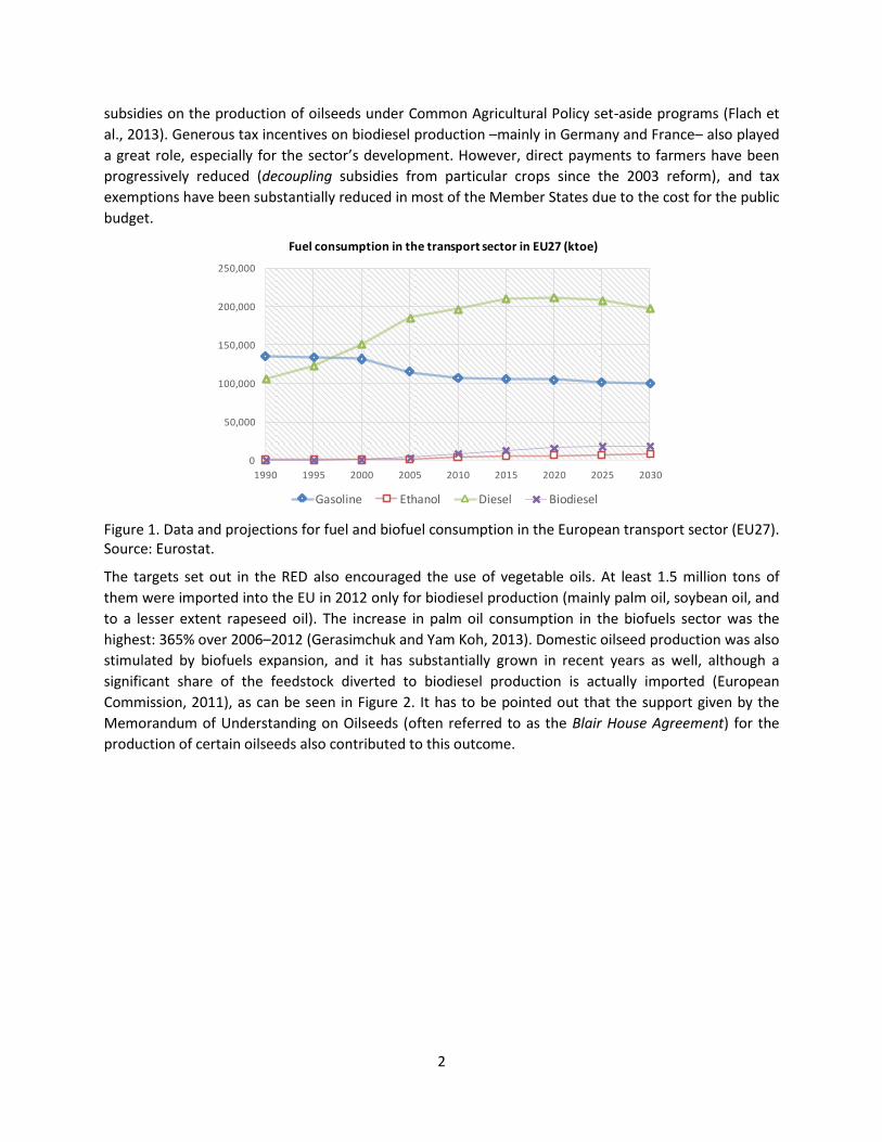
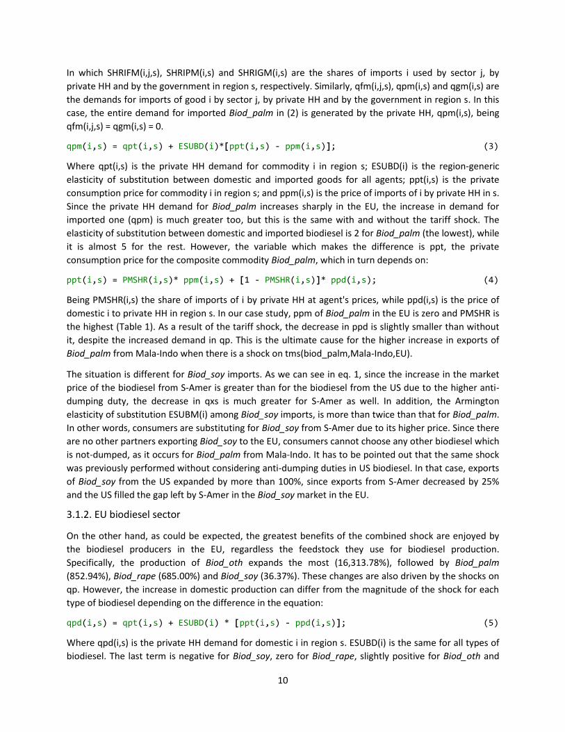
The targets set out in the RED also encouraged the use of vegetable oils. At least 1.5 million tons of

them were imported into the EU in 2012 only for biodiesel production (mainly palm oil, soybean oil, and

to a lesser extent rapeseed oil). The increase in palm oil consumption in the biofuels sector was the

highest: 365% over 2006–2012 (Gerasimchuk and Yam Koh, 2013). Domestic oilseed production was also

stimulated by biofuels expansion, and it has substantially grown in recent years as well, although a

significant share of the feedstock diverted to biodiesel production is actually imported (European

Commission, 2011), as can be seen in Figure 2. It has to be pointed out that the support given by the

Memorandum of Understanding on Oilseeds (often referred to as the Blair House Agreement) for the

production of certain oilseeds also contributed to this outcome.

0

50,000

100,000

150,000

200,000

250,000

1990 1995 2000 2005 2010 2015 2020 2025 2030

Fuel consumption in the transport sector in EU27 (ktoe)

Gasoline Ethanol Diesel Biodiesel

3

Figure 2. Evolution in biodiesel consumption, production and net imports in the European transport

sector (EU27). Net imports of oilseeds into the EU are also represented, although uses other than

biodiesel production are considered. Source: FAPRI.

Possibly driven by all these factors, the EU is currently the world’s largest biodiesel producer. Biodiesel is

also the most important biofuel and, on volume basis, represents about 80% of the total transport

biofuels market (Hélaine, M’barek and Gay, 2013), in the same way that diesel prevails over gas in the

motor fuel market. However, according to Flach et al. (2013), EU biodiesel consumption seems to have

reached its peak after years of rapid increases. In addition, despite this huge demand for biodiesel,

imports represent a large share (around 50%) since biodiesel from leading exporting countries is very

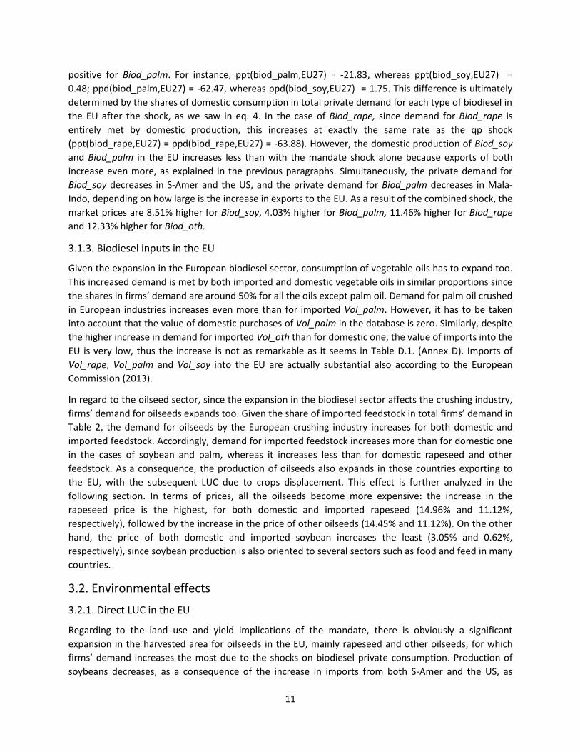
competitive and usually cheaper than domestic biodiesel. In March 2009, the European Commission (EC)

had to impose anti-dumping duties on all the biodiesel blends imported from the United States (US)

(Regulation 444/2011), after having set provisional measures on B20 blends (Regulation 193/2009). As a

consequence, biodiesel imports from Argentina and Indonesia took the US market share and have been

growing since then, as shown in Figure 3. These two countries, very export-oriented, currently account

for almost 40% of the total biodiesel imports into the EU (European Commission, 2013). The EU

accounts for approximately 88% of the total biodiesel exports from Indonesia (Slette and Wiyono, 2013).

In view of this situation, and after investigation, the EC has recently approved anti-dumping duties on

biodiesel imports from both Argentina and Indonesia (Regulation 490/2013), and overall EU biodiesel

imports are expected to almost half in 2013 (Flach et al., 2013).

-5,000

0

5,000

10,000

15,000

20,000

25,000

30,000

2000 2005 2010 2015 2020 2025

Biodiesel commodities in the EU (thounsads Tm)

Biodiesel consumption Biodiesel Production Biodiesel net imports

Palm oil consumption Palm oil net imports Soybean oil consumption

Soybean oil net imports Soybeans consumption (crushing) Soybeans net imports

Rapeseed consumption (crushing) Rapeseed net imports

4

Figure 3. Biodiesel imports from Argentina and Indonesia. Effect of the anti-dumping duties on biodiesel

from the US in 2009. Source: European Biodiesel Board (EBB).

Furthermore, besides the constraint imposed by the sustainability requirements laid down in the RED

for both domestic and imported biodiesel, the EC recently published a new proposal, known as COM 595

(European Commission, 2012), which still has to be ratified. The proposal aims at starting the transition

to biofuels made from non-food feedstock, since first generation biofuels (FGBs) –or biofuels

manufactured from biomass which is generally edible– can negate the environmental benefits as

compared to the fossil fuels they replace. This is meant to be done by setting a cap on, while phasing out

of public support for FGBs after 2020 and establishing a GHG saving requirement of at least 60 percent

for new installations. After intense debate, it is expected that the contribution of FGBs to the target in

the RED will be limited to 6%. Although this value was initially set at 5%, producers within the rapeseed

biodiesel supply chain of Central Europe still reject this proposal.

The underlying reason of this threshold is to reduce the emissions associated with changes in the carbon

stock of land resulting from biofuels expansion. Specifically, the COM 595 is focused on limiting the

emissions from Indirect Land Use Change (ILUC), which were not subject to reporting requirements

under the previous legislation. This effect is the result of increased consumption of feedstock for biofuel

production in different parts of the world, since previous crops have to be diverted to bioenergy. Apart

from the direct conversion of land to satisfy demand of the Member States, production of energy crops

on current land can induce ILUC elsewhere, since the displaced activities are subject to be implemented

in other regions. In other words, ILUC is the result of global shifts in land cover and crop patterns in

response to price changes, referred to as market-mediated impacts by Hertel and Tyner (2013).

Ultimately, ILUC leads to changes in the carbon stock of the soil and the biomass, modifying the carbon

balance of the land and releasing GHG emissions into the atmosphere (among other social and

economic effects). Hence, the COM 595 urges the Member States to report ILUC values associated to

the biofuels used to meet the 10% target, while providing ILUC factors depending on the feedstock.

However, all the pressure groups such as European farmers, crushers, traders and biofuels producers

reject the ILUC political compromise of the EU (EBB, 2013a,b), even they argue to remove ILUC

considerations of any future Directive (COPA-COGECA, 2012).

Since the first studies warning against the risk of indirect GHG emissions from the biofuels boom

(Fargione et al., 2008; Gibbs et al., 2008; Searchinger et al., 2008), much research work has been

conducted on the ILUC effects from increased demand. While some authors developed different

5

accounting methods relying on statistical data and methodological assumptions (Kim and Dale, 2011;

Overmars et al., 2011), most of the latest studies agree on the use of Computable General Equilibrium

(CGE) models, due to the global dimension of the bioenergy development. These are based on model

projections of future responses rather than on historical observations. Specifically, the Global Trade

Analysis Project (GTAP) (Hertel, 1997) has been broadly used in the study of ILUC responses, since

Taheripour et al. (2007) introduced biofuel commodities in the version 6 of the GTAP database. This

model provided the basis for further improvement and yielded a large number of studies addressing

ILUC mainly due to US and EU policies (Banse et al., 2008; Hertel et al., 2010; Kløverpris, Baltzer and

Nielsen, 2010; Taheripour et al., 2010; Taheripour et al., 2012). They consider that biofuel targets will be

met by both land and yield adjustments, proving that significant changes in land use are expected to

occur not only in those countries driving the demand for biofuels, but also in other parts of the world

due to the interaction among agricultural-biofuel markets. In fact, one of the largest sources of potential

GHG emissions associated with biofuels production results from the ILUC, which will take place in

different regions of Latin America, Asia or Africa. Although the recent study of the EBB (Darlington et al.,

2013) used a version of the GTAP database to calculate land conversion and ILUC emissions from

increased consumption of FGBs in the EU according to an 8.75% target -as projected for 2015-, the

effects of the COM 595 together with the anti-dumping duties have not been studied yet. Similarly, Al-

Riffai, Dimaranan and Laborde (2010) applied the MIRAGE model, based on the GTAP 7 database

(Narayanan and Walmsley, 2008), to analyze the interaction between a 5.6% target for FGBs in 2020 and

trade liberalization measures on imports from the MERCOSUR countries, also in terms of LUC effects.

In the light of a growing concern about the ILUC effects of the biofuels expansion, the objective of the

present study is thus to analyze the global environmental consequences of these different strategies

recently proposed by the EC to stimulate the domestic biodiesel production while reducing GHG

emissions. One single experiment is performed to get the full picture of how the market will react to the

new cap on FGBs and the existing anti-dumping measures on biodiesel from Argentina, Indonesia and

the US. It is found that LUC will take place not only in the EU but also at a global scale as a consequence

of biodiesel trade and interactions in the food and feed markets. While the US gains of market share at

the expense of Argentina, exports of palm biodiesel from Malaysia and Indonesia to the EU are even

fostered by the increase in the import price, since European consumers continue to depend on them to

meet the targets. Biodiesel producers in the EU benefit from these policies as well, especially those

producing rapeseed and non-food-based biodiesel, for which the increase in demand is the highest. The

expansion in the European biodiesel sector triggers demand for both vegetable oils and oilseeds,

altering crop patterns in other countries not directly affected through biodiesel trade relations. As a

result, not even the biodiesel self-sufficiency is completely achieved, since the EU needs to import

biodiesel feedstock, while global GHG emissions from LUC significantly increase. This paper is organized

into the following sections: Section 2 describes methodology; results are analyzed and discussed in

Section 3, in regard to market responses and environmental effects; finally, conclusions are drawn in

Section 4, providing insights for further improvement.

2. Methodology

2.1. The GTAP-BIO version

A version of the standard GTAP model (Hertel, 1997) has been used. Specifically, the latest version of

the GTAP-BIO, described by Golub and Hertel (2012), and built on the version of Birur, Hertel and Tyner

6

(2008). This version modified the GTAP-E model (Burniaux and Truong, 2002), whose main contribution

was to incorporate energy substitution in the production nest by allowing capital and energy to be

either substitutes or complements. Substitution follows a nested CES function, based on the separability

between primary factors and intermediate inputs (Figure A.1., Annex A). The energy inputs are

aggregated with capital in a composite, allowing for capital-energy substitution with other factors. The

separability assumption in the standard model was then relaxed to make labor-energy substitution

different from capital-energy in the value added sub-nest. The non-electric intermediate inputs include

petroleum-based fuels. Carbon emissions from the combustion of them are included too, as well as a

mechanism to trade these emissions internationally.

The GTAP-E version was extended by McDougall and Golub (2007) to improve its applicability to a wider

range of energy-environmental policy scenarios. Taheripour et al. (2007) further modified it to

incorporate the potential for biofuels to substitute for petroleum products. Biofuel commodities were

included, based on the International Energy Agency (IEA) database and plant-level, biofuel processing

models. As a result, three biofuel sectors were included: ethanol from coarse grains, ethanol from

sugarcane and biodiesel from oilseeds. In addition, the model includes Dried Grains with Solubles

(DDGS) as a byproduct of corn-based ethanol production and protein meals from biodiesel production,

which can displace other protein sources for animal feed (with the subsequent consequences on the

feed market). As Golub and Hertel (2012) commented on this version, the prominence given to energy

substitution makes it a very useful tool for the study of biofuel mandates implications, since the

mandate will be more costly for the economy if alternative fuels are not good substitutes for petroleum

products and the other way round. Finally, Birur, Hertel and Tyner (2008) took advantage of these

feature implementations in order to associate land use information to biofuels consumption.

Specifically, they implemented a land use module allowing to estimate LUC in different agroecological

zones (AEZ) and the associated emissions. By using the GTAP land use database developed by Lee et al.

(2005), 18 AEZs were defined according to two dimensions: growing period (6 categories of 60 day

growing period intervals) and climatic zones (3 categories: tropical, temperate and boreal). The

competition for land within a given AEZ across uses, triggered by biofuel policies, is modeled in this way,

based on historical observations to determine which activities have been observed to take place in each

AEZ.

The latest GTAP-BIO version is in turn based on the version 8 of GTAP database, depicting the world

economy in 2004. It is similar to the one created by Taheripour et al. (2011) (GTAP-BIO-ADV) but the

feature that makes it more interesting for our analysis is that this particular version disaggregates

biodiesel into soybean biodiesel, rapeseed biodiesel, palm biodiesel and biodiesel from other feedstock

(Biod_soy, Biod_rape, Biod_palm and Biod_oth) (as explained in Figure B.1., Annex B). Four different

agricultural commodities (soybeans, rapeseed, palm and other oilseeds) are considered for biodiesel

production as well, and these four agricultural industries compete in land, capital, labor, and

intermediates, and sell their products to other industries (mainly vegetable oil, food and feed industries)

and households (HH). The vegetable oil industry in GTAP is thus divided accordingly into Vol_soy,

Vol_rape, Vol_palm and Vol_oth. Substitution among all these types of vegetable oils in the HH and firm

demand for goods and services is possible thanks to a new elasticity parameter. This tries to represent

how demand for oils shifts to cheaper oils when the price of one particular type of oil increases sharply

as a consequence of the increased demand by biodiesel firms. It is assigned a high value in the regions

which produce different oilseeds or import them from other regions (e.g. China and EU members), while

7

is small in the regions which mainly produce one type of vegetable oil (e.g. Brazil and the US). As a

result, the database covers 19 regions, 42 industries and 48 commodities, as is shown in Table C.1.

(Annex C).The land use module allows competition among traditional crops and dedicated energy crops

for idle land and cropland pasture. Among other characteristics, it offers greater flexibility in acreage

switching among uses in response to price changes and includes an endogenous yield adjustment for

cropland pasture (which represents marginal land previously used for agriculture) in response to

changes in cropland pasture rent but only for the US and Brazil; other regions do not have this

possibility. The ratio of marginal and average productivities (ETA), which measures the productivity of

new cropland versus the productivity of existing cropland, now varies across regions and among AEZs.

2.2. Intensive and extensive margins

As the version used by Hertel et al. (2010), this version models the changes in the intensive and

extensive margins of yield responses due to increased biofuels demand. Whereas the intensive margin

captures the increase in yields as a response of higher prices of agricultural commodities, the extensive

margin is defined as the change in yield when land employed in other uses (crop, pasture or forest) is

converted to grow oilseeds. If oilseeds production expands onto lower productivity land, then the

extensive margin will be negative, capturing the tendency to reduce yields as less productive land -even

idle land- must be brought into production.

In regard to the extensive margin, two main causes are considered: when demand for oilseeds increases,

other crops can be displaced on existing agricultural land. This displacement is estimated from the

differential in net returns to land in existing uses, based on the assumption that land will be allocated to

its highest value use. A nested CET structure of land supply is implemented (Ahammad and Mim 2005)

whereby the land owner first decides on the allocation of land among three uses (forest, cropland and

pasture) in order to maximize his rent. The second cause arises from the change in average crop yields

as cropland area is expanded into land not previously used for agricultural purposes, such as pasture or

forest. The extensive margin is determined by the ETA parameter (elasticity of output with respect to

acreage expansion), which varies between 0.42 and 1 depending on the region and the AEZ. The lowest

value means that diverting three hectares of current cropland to biofuel feedstock production takes

seven additional hectares of marginal land (cropland pasture), implying the lowest productivity of the

land which can be potentially diverted for biofuels production. On the contrary, if ETA is 1, the

converted land has the same productivity as existing cropland in that AEZ, such as the case of other

crops. Each land conversion in each AEZ is assigned a CO2 emission factor (based on estimations of the

California Air Resources Board) in the land use module.

2.3. Closure and shocks

The standard GE closure has been used. The policy experiment presented has been inspired by the

policies mentioned in the introduction (the new proposal COM 595, and the Regulations 444/2011 and

490/2013), and based on statistical data and energy projections from Eurostat (2013). The ratio ethanol-

biodiesel calculated is around 3/8 for 2020.

One single experiment has been performed, in order to shock simultaneously: 1) increased biodiesel

consumption due to the new target for FGBs (6%); 2) increase in the CIF price of biodiesel imports into

the EU from Southeastern Asia (Mala-Indo) by 18.9%, from South America –excluding Brazil– (S-Amer)

by 24.6% and from the US by 10.8%, and see how these policies interact in the same time frame. For 1),

8

private demand for Biod_soy, Biod_rape and Biod_palm has been expanded by using current shares on

first generation biodiesel consumption in the EU (26.3%, 56.2% and 12.3%, respectively), while Biod_oth

has been increased according to the remaining 4% target in the COM 595. Bilateral trade flows of

Biod_soy, Biod_palm and Biod_oth between the EU27 and the main exporting regions were previously

introduced by using the Altertax closure (documented in Malcolm, 1998), according to data reported by

Lamers et al. (2011). Biodiesel production and consumption in the EU were updated in the initial dataset

as well. All the shocks and swaps for this experiment are summarized in Table 1. It has to be pointed out

that the sharp increase in demand for Biod_oth is due to very low consumption levels in the base data

together with the projected consumption in 2020 (3.03 thousand million gallons).

Table 1. Shock statements to perform the experiment.

Shocks and swaps statements

swap del_taxrpcbio("EU27") = tpbio("EU27")1 -

swap qp("biod_soy","EU27") = tpd("biod_soy","EU27") -

swap qp("biod_palm","EU27") = tpd("biod_Palm","EU27") -

swap qp("biod_rape","EU27") = tpd("biod_Rape","EU27") -

swap qp("biod_oth","EU27") = tpd("biod_Oth","EU27") -

shock qp("biod_rape","EU27") 685.0

shock qp("biod_palm","EU27") 119.6

shock qp("biod_soy","EU27") 45.12

shock qp("biod_oth","EU27") 7327.8

shock tms("biod_palm","Mala-Indo","EU27") 18.9

shock tms("biod_soy","S-Amer","EU27") 24.6

shock tms("biod_soy","USA","EU27") 10.8

3. Results

Market responses have been estimated by analyzing changes in the most significant variables (shown in

Table D.1., Annex D), as compared to the same changes without the anti-dumping measures. Changes in

the harvested area in the regions directly affected by the policy measures are shown in Table 3 (EU-27),

Table 4 (S-Amer), Table 5 (US) and Table 6 (Mala-Indo). Extensive and intensive margins have been

analyzed separately for each of these regions and for different agricultural commodities competing with

biodiesel feedstock for land.

3.1. Market responses through the biodiesel supply chain

3.1.1. Biodiesel imports

As was mentioned previously, biodiesel imports into the EU have been updated until they reached 2009

levels by using the Altertax closure (Malcolm, 1998), in order not to underestimate the global effects of

the blending mandate arising from bilateral trade. However, these trade flows involve only major

biodiesel exporters to the EU, which were Argentina, the US, Indonesia, Canada and Malaysia in 2009,

according to Lamers et al. (2011). The consumption share of imported biodiesel relative to domestic one

has then changed from less than 0.05% for Biod_soy, Biod_palm and Biod_oth to 78.48%, 83.23% and

47.06%, respectively, depicting a more realistic situation. The share of imported Biod_rape has remained

around 0%, which is consistent with current consumption patterns in the EU. On the contrary, the shares

1 This statement prevents the tax revenue for the government from being affected when tpbio adjusts for allowing qp to change, by evenly

distributing the tax changes across all biofuels. Tpbio is a tax to implement a blending mandate, originally created for the LCFS.

9

of imported oils in biodiesel firms’ demand are around 50% for soybean, palm and rape, whereas the

entire demand for palm oil is met with imported oil. All these shares are summarized in Table 2. Overall,

S-Amer accounts for 10.9% of the EU private consumption of biodiesel, while the US and Mala-Indo

account for 6.1% and 3.5%, respectively.

Table 2. Import share within the biodiesel supply chain in the EU-27

Share of imported biodiesel in HH

demand

Share of imported oils in biodiesel firms' demand

Share of imported oilseeds in crushing industries’ demand

Soy 78.5% 50.3% 96.6%

Palm 83.2% 100.0% 97.4%

Rape 0.0% 49.6% 36.1%

Others 47.1% 49.6% 43.2%

By applying the updated shares, the expansion in demand for biodiesel in the EU following the

requirements in the COM 595 is met by both, imports and domestic production. In this section, the

experiment results may be compared to results arising from the mandate shock alone for further

interpretation. Without the tariff shock, the increased demand for soybean biodiesel causes an increase

in exports from S-Amer (67.29%), while exports from the US only expand by 2.70%. In addition, imports

from other European countries increase by 426.77%, from both imported and domestic soybeans. The

corresponding shock on EU demand for palm biodiesel increases exports from Mala-Indo by 32.79%.

Since this is the only biodiesel source of palm biodiesel to the EU, these two countries account for the

entire import share in the European market in the database. Even introducing the tariff shock, exports

from these three countries to the EU expand, triggered by the sharp increase in private consumption. As

can be observed in Table D.1. (Annex D), imports from S-Amer increase less (24.91%) due to the anti-

dumping duties, which are the highest for that country of origin. The expansion in exports from Mala-

Indo is slightly greater (34.19%), while exports of soybean biodiesel from the US increase much more

(93.20%), since they take part of the S-Amer’s market share despite the anti-dumping duties on its own

exports. It can be said that the anti-dumping duties have the most detrimental consequences on

soybean biodiesel exports from S-Amer, since these consequences are determined in accordance of the

shock on tms.

To explain the consequences of the tariff shocks on biodiesel exports from Mala-Indo, the US and S-

Amer, we should look at the equations used to explain exports from each country in the model:

qxs(i,r,s)= qim(i,s) - ESUBM(i)*[pms(i,r,s)- pim(i,s)]; (1)

Where qxs(i,r,s) are the export sales of commodity i from r to region s; qim(i,s) are the aggregate

imports of i in region s (weighted according to market prices); ESUBM(i) is the region-generic elasticity of

substitution among imports of i in Armington structure; pms(i,r,s) is the domestic price for good i

supplied from r to region s; and pim(i,s) is the market price of composite import i in region r.

Since Mala-Indo enjoys a share of 100% for Biod_palm imports into the EU, the third term in (1) goes to

zero and qxs(i,r,s) = qim(i,s). In the market clearing equation for imported Biod_palm entering the EU:

qim(i,s) = sum(j,ALL_INDS,SHRIFM(i,j,s)* qfm(i,j,s)) + SHRIPM(i,s)* qpm(i,s) +

SHRIGM(i,s)* qgm(i,s); (2)

10

In which SHRIFM(i,j,s), SHRIPM(i,s) and SHRIGM(i,s) are the shares of imports i used by sector j, by

private HH and by the government in region s, respectively. Similarly, qfm(i,j,s), qpm(i,s) and qgm(i,s) are

the demands for imports of good i by sector j, by private HH and by the government in region s. In this

case, the entire demand for imported Biod_palm in (2) is generated by the private HH, qpm(i,s), being

qfm(i,j,s) = qgm(i,s) = 0.

qpm(i,s) = qpt(i,s) + ESUBD(i)*[ppt(i,s) - ppm(i,s)]; (3)

Where qpt(i,s) is the private HH demand for commodity i in region s; ESUBD(i) is the region-generic

elasticity of substitution between domestic and imported goods for all agents; ppt(i,s) is the private

consumption price for commodity i in region s; and ppm(i,s) is the price of imports of i by private HH in s.

Since the private HH demand for Biod_palm increases sharply in the EU, the increase in demand for

imported one (qpm) is much greater too, but this is the same with and without the tariff shock. The

elasticity of substitution between domestic and imported biodiesel is 2 for Biod_palm (the lowest), while

it is almost 5 for the rest. However, the variable which makes the difference is ppt, the private

consumption price for the composite commodity Biod_palm, which in turn depends on:

ppt(i,s) = PMSHR(i,s)* ppm(i,s) + [1 - PMSHR(i,s)]* ppd(i,s); (4)

Being PMSHR(i,s) the share of imports of i by private HH at agent's prices, while ppd(i,s) is the price of

domestic i to private HH in region s. In our case study, ppm of Biod_palm in the EU is zero and PMSHR is

the highest (Table 1). As a result of the tariff shock, the decrease in ppd is slightly smaller than without

it, despite the increased demand in qp. This is the ultimate cause for the higher increase in exports of

Biod_palm from Mala-Indo when there is a shock on tms(biod_palm,Mala-Indo,EU).

The situation is different for Biod_soy imports. As we can see in eq. 1, since the increase in the market

price of the biodiesel from S-Amer is greater than for the biodiesel from the US due to the higher anti-

dumping duty, the decrease in qxs is much greater for S-Amer as well. In addition, the Armington

elasticity of substitution ESUBM(i) among Biod_soy imports, is more than twice than that for Biod_palm.

In other words, consumers are substituting for Biod_soy from S-Amer due to its higher price. Since there

are no other partners exporting Biod_soy to the EU, consumers cannot choose any other biodiesel which

is not-dumped, as it occurs for Biod_palm from Mala-Indo. It has to be pointed out that the same shock

was previously performed without considering anti-dumping duties in US biodiesel. In that case, exports

of Biod_soy from the US expanded by more than 100%, since exports from S-Amer decreased by 25%

and the US filled the gap left by S-Amer in the Biod_soy market in the EU.

3.1.2. EU biodiesel sector

On the other hand, as could be expected, the greatest benefits of the combined shock are enjoyed by

the biodiesel producers in the EU, regardless the feedstock they use for biodiesel production.

Specifically, the production of Biod_oth expands the most (16,313.78%), followed by Biod_palm

(852.94%), Biod_rape (685.00%) and Biod_soy (36.37%). These changes are also driven by the shocks on

qp. However, the increase in domestic production can differ from the magnitude of the shock for each

type of biodiesel depending on the difference in the equation:

qpd(i,s) = qpt(i,s) + ESUBD(i) * [ppt(i,s) - ppd(i,s)]; (5)

Where qpd(i,s) is the private HH demand for domestic i in region s. ESUBD(i) is the same for all types of

biodiesel. The last term is negative for Biod_soy, zero for Biod_rape, slightly positive for Biod_oth and

11

positive for Biod_palm. For instance, ppt(biod_palm,EU27) = -21.83, whereas ppt(biod_soy,EU27) =

0.48; ppd(biod_palm,EU27) = -62.47, whereas ppd(biod_soy,EU27) = 1.75. This difference is ultimately

determined by the shares of domestic consumption in total private demand for each type of biodiesel in

the EU after the shock, as we saw in eq. 4. In the case of Biod_rape, since demand for Biod_rape is

entirely met by domestic production, this increases at exactly the same rate as the qp shock

(ppt(biod_rape,EU27) = ppd(biod_rape,EU27) = -63.88). However, the domestic production of Biod_soy

and Biod_palm in the EU increases less than with the mandate shock alone because exports of both

increase even more, as explained in the previous paragraphs. Simultaneously, the private demand for

Biod_soy decreases in S-Amer and the US, and the private demand for Biod_palm decreases in Mala-

Indo, depending on how large is the increase in exports to the EU. As a result of the combined shock, the

market prices are 8.51% higher for Biod_soy, 4.03% higher for Biod_palm, 11.46% higher for Biod_rape

and 12.33% higher for Biod_oth.

3.1.3. Biodiesel inputs in the EU

Given the expansion in the European biodiesel sector, consumption of vegetable oils has to expand too.

This increased demand is met by both imported and domestic vegetable oils in similar proportions since

the shares in firms’ demand are around 50% for all the oils except palm oil. Demand for palm oil crushed

in European industries increases even more than for imported Vol_palm. However, it has to be taken

into account that the value of domestic purchases of Vol_palm in the database is zero. Similarly, despite

the higher increase in demand for imported Vol_oth than for domestic one, the value of imports into the

EU is very low, thus the increase is not as remarkable as it seems in Table D.1. (Annex D). Imports of

Vol_rape, Vol_palm and Vol_soy into the EU are actually substantial also according to the European

Commission (2013).

In regard to the oilseed sector, since the expansion in the biodiesel sector affects the crushing industry,

firms’ demand for oilseeds expands too. Given the share of imported feedstock in total firms’ demand in

Table 2, the demand for oilseeds by the European crushing industry increases for both domestic and

imported feedstock. Accordingly, demand for imported feedstock increases more than for domestic one

in the cases of soybean and palm, whereas it increases less than for domestic rapeseed and other

feedstock. As a consequence, the production of oilseeds also expands in those countries exporting to

the EU, with the subsequent LUC due to crops displacement. This effect is further analyzed in the

following section. In terms of prices, all the oilseeds become more expensive: the increase in the

rapeseed price is the highest, for both domestic and imported rapeseed (14.96% and 11.12%,

respectively), followed by the increase in the price of other oilseeds (14.45% and 11.12%). On the other

hand, the price of both domestic and imported soybean increases the least (3.05% and 0.62%,

respectively), since soybean production is also oriented to several sectors such as food and feed in many

countries.

3.2. Environmental effects

3.2.1. Direct LUC in the EU

Regarding to the land use and yield implications of the mandate, there is obviously a significant

expansion in the harvested area for oilseeds in the EU, mainly rapeseed and other oilseeds, for which

firms’ demand increases the most due to the shocks on biodiesel private consumption. Production of

soybeans decreases, as a consequence of the increase in imports from both S-Amer and the US, as

12

discussed in the previous section. Even if the model’s output shows an increase in the production of

palm, it has to be pointed out that the initial level of production in the database is zero. As can be seen

in Table 3, 52.84% more land is diverted to rapeseed and 52.18% is diverted to other oilseeds. This

expansion takes place not only at the expense of soybean (which is not a widespread crop in the EU) but

also at the expense of other crops, especially paddy rice, wheat, other coarse grains and other crops.

However, these four commodities still account for 80.2% of the overall agricultural land in the EU.

Higher oilseeds prices lead to higher yields under the intensive margin. There is also a significant yield

adjustment in the rest of the crops for which area is contracting, in order to avoid greater production

slowdowns. The extensive margin prevails though, which is positive in this case, suggesting that in much

of the EU the productivity of land that might be converted to cropland is about the same as existing

cropland. This happens because LUC takes place at the cost of land previously used for agricultural

production and not from idle land, as shown in Table 3. Indeed, neither pasture nor other agri-industrial

sectors are affected. These values are mostly the result of the shock on biodiesel consumption and

hardly change due to the tariff shock.

Table 3. Change in harvested area by crop for the EU-27

Soybeans Rapeseed Palm Other

oilseeds Wheat Sorghum

Other coarse grains

Paddy rice Sugarcane

Other crops

Decomposition of output changes (%)

Output -7.76 61.10 15.51 61.48 -3.50 1.09 -0.33 -4.79 -0.70 -2.80

Yield 4.43 5.40 0.00 6.10 4.54 4.80 4.94 4.72 4.58 4.63

Area -11.69 52.84 0.00 52.18 -7.41 -3.55 -5.03 -9.16 -4.90 -6.89

Decomposition of yield changes (%)

Yield 4.40 5.33 0.00 6.02 4.51 4.76 4.89 4.70 4.54 4.59

Intensive margin 0.60 1.90 0.00 1.95 0.87 1.18 1.18 0.68 0.97 1.01

Extensive margin 3.80 3.43 0.00 4.07 3.64 3.58 3.71 4.02 3.57 3.58

Harvested area (Mha) 0.35 6.83 0.00 13.60 24.51 0.10 32.05 0.39 2.12 35.94

3.2.2. Global LUC and GHG emissions

The effects in the biodiesel exporting countries are similar. There is an increase in the land dedicated to

rapeseed and other oilseeds in the three regions, although it has to be pointed out that Mala-Indo does

not produce rapeseed. This is a result of the huge expansion in demand for these oilseeds by the

European crushing industries, but also the expansion in domestic demand to produce biodiesel for

export. On the contrary, the production of soybean decreases to meet this greater demand for other

oilseeds. This suggests that part of the available soybeans is no longer used in other sectors in the US

and S-Amer, in order to increase Biod_soy exports to the EU. In fact, oilseeds demand by other

important sectors decreases in these two countries, mainly livestock and feed processing industries. The

area diverted to palm in S-Amer expands as well, to increase exports of Vol_palm to the European

market. Other LUC effects can be observed for S-Amer: the area diverted to most of coarse grains

decreases (except for other coarse grains) and the intensive margin still prevails, even if the converted

land is, in some cases, less productive for current uses than for the previous ones. However, LUC effects

in S-Amer are the least remarkable, since demand for oilseeds is much diversified across sectors, and the

effect of the increased demand for biodiesel is diluted; the livestock sector is indeed very important in

13

countries such as Argentina. In the US, production of all the coarse grains expands at the expense of idle

land and pasture, and that is why yields decrease. It has to be recalled though that transformation from

pasture is only possible in the model for the US and Brazil. Finally, in Mala-Indo, production of palm

increases the most, while the increase in rapeseed production is not relevant because it is initially zero.

As can be seen in Table 6, the resulting area dedicated to rapeseed, wheat and sorghum is zero in Mala-

Indo, whereas only palm and rice account for 60.2% of the total acreage in the region. As a

consequence, the land used for the rest of crops must decrease, except for other oilseeds. The intensive

margin again determines the subsequent yield adjustments, while the extensive margin is negative

leading to the conclusion that the new cropland is less productive, coming at the expense of degraded

land (due to overdrainage) or anthropogenic grassland, with high acidity level and low content of

organic matter (Chouychai et al., 2009; Germer and Sauerborn, 2008).

Despite the changes in crop patterns, overall GHG emissions in Table 7 show that the sharp expansion in

worldwide oilseeds production not only takes place at the expense of other crops but also from land

used for other activities. These GHG emissions are calculated by multiplying the acreage changes by the

calculated CO2 emission factors. Whereas transformation from arable land leads to carbon uptake in all

the analyzed regions (since the new crops improve the GHG balance as compared to the previous ones),

contraction in the area diverted to livestock and especially forestry generates substantial GHG

emissions, with the subsequent global warming impact. This is the result of higher emission factors

associated with transformation from grassland or forest to crops in each AEZ, since there are CO2

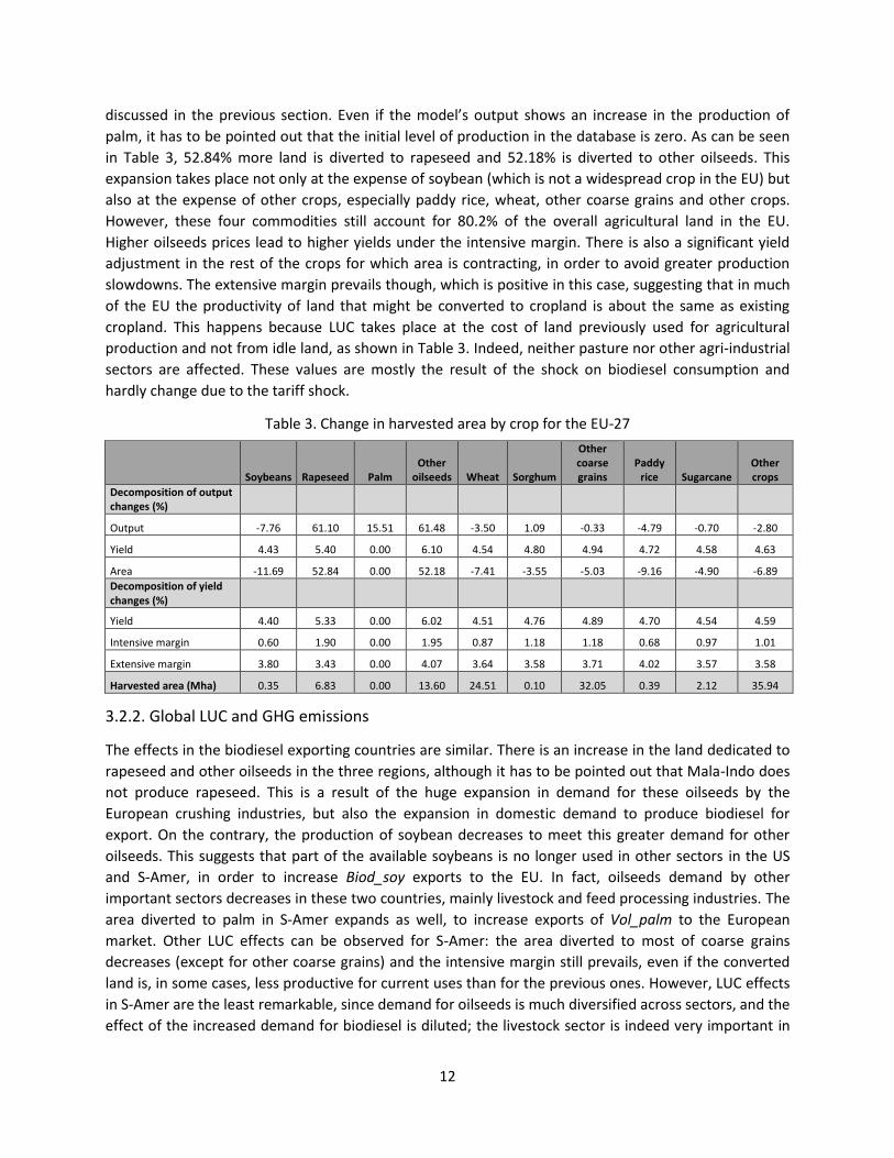
emissions arising from changes in the carbon stock in soil and biomass. Finally, Figure 4 shows absolute

changes in the distribution of the global agricultural land, by crop and region, as a consequence of the

shock on biodiesel consumption in the EU by 2020. Apart from the LUC effects outlined in previous

paragraphs, the expansion in acreage in Sub-Saharan Africa (SS-Africa), Brazil, other CEE countries,

Russia and Canada is also remarkable, mainly to produce other oilseeds and rapeseed for export to the

EU, or palm to produce oil for export too (e.g. in SS-Africa). As a result of the increased demand for

biodiesel in the EU, overall LUC by 2020 will lead to an expansion in the worldwide agricultural land of

3.24 Mha, whereas area dedicated to oilseeds, cereals and sugarcane will increase by 6.50 Mha.

Similarly, in the EU, there will be an increase of 7.01 Mha in the acreage for rapeseed and other oilseeds,

which will partially take place at the expense of 6.76 Mha from other crops, wheat or other coarse

grains, causing a net expansion of 0.25 Mha in the agricultural land, only surpassed by the expansion in

Brazil and SS-Africa.

Table 4. Change in harvested area by crop for S-Amer



Other coarse grains


Other crops


Output -2.85 29.27 32.04 26.98 -0.67 0.46 0.74 -0.26 -0.18 0.54

Yield -0.01 2.12 3.19 2.38 0.26 0.51 0.50 0.87 0.79 0.65

Area -2.84 26.59 27.96 24.03 -0.99 -0.05 0.24 -1.04 -0.91 -0.21


Yield 0.00 2.12 3.18 2.38 0.26 0.51 0.50 0.87 0.78 0.65


Extensive margin -0.27 -0.28 0.48 -0.05 -0.23 -0.06 -0.09 0.29 0.29 -0.03


14

Table 5. Change in harvested area by crop for the US



Other coarse grains


Other crops


Output -4.74 40.68 3.84 32.73 2.50 0.26 0.52 0.51 -0.01 0.73

Yield -0.73 1.60 0.00 1.11 -0.06 -0.33 -0.41 -0.68 -0.27 -0.21

Area -4.05 38.47 0.00 31.27 2.56 0.59 0.93 1.19 0.25 1.03


Yield -0.73 1.60 0.00 1.13 -0.06 -0.33 -0.40 -0.67 -0.26 -0.21


Extensive margin -0.76 -0.28 0.00 -0.62 -0.50 -0.61 -0.67 -0.99 -0.68 -0.58


Table 6. Change in harvested area by crop for Mala-Indo



Other coarse grains


Other crops


Output -1.13 19.08 5.14 0.75 3.68 -2.22 -0.58 -0.44 -0.30 -0.27

Yield -0.11 0.00 1.56 0.43 0.00 0.00 0.09 0.15 0.23 0.25

Area -1.03 0.00 3.53 0.32 0.00 0.00 -0.68 -0.58 -0.50 -0.45


Yield -0.11 0.00 1.56 0.44 0.00 0.00 0.09 0.15 0.24 0.25


Extensive margin -0.23 0.00 -0.29 -0.28 0.00 0.00 -0.24 -0.25 -0.28 -0.27


Table 7. Global GHG emissions from LUC (Tg of CO2-eq.)

Forestry Crops Livestock Total

In EU 46.71 -4.54 14.08 56.25

In Mala-Indo 83.20 -1.84 0.99 82.18

In S-Amer -5.41 -2.11 10.58 3.07

USA 16.29 -1.12 42.43 57.59

Rest of the world 426.31 -51.25 101.44 476.50

15

Figure 4. Changes in total agricultural land (Mha), by region, due to the shock on biodiesel consumption in the EU with the subsequent anti-dumping duties. Other countries than the main biodiesel exporters to the EU are affected by means of interactions among other agricultural commodities in the global market, triggered by changes across the biodiesel supply chain.

4. Conclusions

The results obtained show that establishing a 6% target for FGBs and a 4% target for advanced biofuels

(with or without anti-dumping measures) is a great incentive for the biodiesel sector in the EU, since the

market is filled with imported biodiesel but also with domestic product. Specifically, domestic

production of Biod_rape and Biod_oth increases sharply. Despite the anti-dumping measures on

biodiesel imports from Mala-Indo, the US and S-Amer, exports from these origins expand too, due to the

huge increase in EU private demand for biodiesel, which obviously affects the leading exporting

countries. When anti-dumping measures are introduced, Biod_palm imports from Mala-Indo into the EU

are even higher due to price responses. In short, if EU has to increase demand for Biod_palm, the only

source for it is Mala-Indo, therefore despite anti-dumping duties and huge tariff increases, EU continues

depending on them. On the contrary, European consumers can choose between Biod_soy from the US

and from S-Amer to meet the mandate targets. Hence, imports of the cheapest Biod_soy increase, which

is the one from the US, due to lower anti-dumping duties as compared to the ones set for S-Amer.

The expansion in demand for biodiesel creates in turn an increased demand for feedstock, not only in

the EU but also in the main exporters of both vegetable oils (such as Mala-Indo, S-Amer, Brazil or India)

and oilseeds (such as USA, Brazil, S-Amer, China or Canada). Feedstock exporting countries are generally

those exporting biodiesel too, since they produce oilseeds and oils for export or for domestic firms’

consumption, depending on the world market prices of each commodity. It has to be pointed out that,

whereas the US and specially S-Amer export both oilseeds and oils, Mala-Indo only exports palm oil, due

to high transportation costs of the fresh palm fruit bunches; this helps to promote the domestic crushing

-8 -6 -4 -2 0 2 4 6 8

Oth-Europe

Japan

E-Asia

Central-Amer

S-Asia

SE-Asia

India

Oceania

Mala-Indo

China-Hongkong

Canada

Russia

S-Amer

Oth-CEE

Brazil

USA

SS-Africa

EU27

Change in cropland extension by region due to the shock (Mha)

Paddy rice Wheat Sorghum Other coarse grains

Soybeans Palm Rapeseed Other oilseeds

Sugarcane Other crops Other agri-industrial uses Pasture

16

industry. Anyhow, the increased demand for biofuels due to European mandates will be only met with

domestic biofuel feedstock partially, and the region will incur an agricultural trade deficit, as Banse et al.

(2008) concluded. LUC will thus take place globally mainly because of the increased production of

rapeseed, palm and other oilseeds, while production of soybean will decrease in major producing

countries since the shock in Biod_soy consumption is the lowest (relative to 2009 consumption levels,

when Biod_soy was the second most used in the EU, after Biod_rape). In addition, in many countries

such as S-Amer, the expansion of these other oilseeds will even occur at the expense of soybean. As has

been addressed, European biofuel policies can have strong consequences outside the EU in terms of LUC

and GHG emissions, mainly in regions such as the US, Brazil, S-Amer but also SS-Africa, Russia or Canada,

by means of market mediated responses. Banse and Grethe (2008) found that increasing EU biofuel

demand –due to the RED– will be satisfied by imports for a substantial share, either in the form of

biofuels or biofuel inputs. These effects will also lead to changes in the agricultural structures

worldwide, which can have other effects than only environmental, for example of social nature. In these

sense, analyzing welfare effects will be useful to estimate the cost of these policies for the society.

It should be recalled, however, that the present results are only based on bilateral trade flows of

biodiesel between the EU and the regions Mala-Indo, S-Amer and the US. As a result, LUC effects are

mainly transferred to other countries via interaction among agricultural markets (ILUC). In order to get a

more realistic picture, the same experiment should be performed by introducing other biofuel trade

flows with all the EU partners. However, current results can be considered reasonably representative

because only Malaysia, Indonesia, Argentina and the US accounted for more than 94% of the total extra-

EU27 biodiesel imports in 2012 (European Commission, 2013). It has to be said that biodiesel production

in the US has slowed down in recent years, and exports to the EU have dramatically declined since 2011,

hardly representing 0.03% of the imports share in 2012. Other countries to be thus considered to

improve the reliability of the analysis should be Norway, South Korea, United Kingdom or Canada,

according to these very data. Similarly, although most of the advanced biodiesel in the EU is currently

produced from domestic used cooking oil (Ecofys et al., 2013), some trade flows of Biod_oth should be

included if consumption of advanced biofuels is expected to increase sharply as a consequence of

policies such as the COM 595, driving demand for imported biodiesel and/or for feedstock (algae,

bagasse, crude glycerin, nut shells, etc). Additionally, it must be noted that for the present experiment,

it has been assumed that the commodity Biod_oth corresponds entirely to advanced biofuels, when in

reality it can be manufactured from other oilseeds such as sunflower, thus competing with food

production. Disaggregating these other FGBs from the Biod_oth commodity would lead to zero LUC

values associated to the increased feedstock production, providing a better analysis of the COM 595

effects. Therefore, current GHG emissions from LUC are overestimated, due to the enormous increase in

the land diverted to other oilseeds. Finally, performing the same experiment by shocking only the

demand for an aggregated first generation biodiesel commodity (including Biod_soy, Biod_rape and

Biod_palm) instead of three independent shocks may provide additional insights, since this will let the

market adjust according to consumers preferences (based on price changes) instead of according to

current consumption shares. Results will then depict projected biodiesel consumption in 2020 through

market mediated responses, and expected LUC and GHG effects may be slightly different in that case.

The fact is that increasing demand for biofuels due to European policies will require the use of a

significant amount of biomass, and the global economy is expected to be affected in several ways, with

the subsequent LUC effects not only in the EU but also in very distant regions. Although these effects are

17

difficult to predict due to their global dimension, addressing LUC is not temporary, and most of the

latest bioenergy policies (such as the Renewable Fuel Standard -RFS2-, RED, etc) urge countries to

reduce overall GHG emissions generated by increasing biofuel consumption. This paper is an example of

the application of the GTAP model to estimate the environmental consequences (regarding to GHG

emissions and ILUC) of different market instruments affecting the biodiesel sector in the EU. When

analyzing public policies, these market mediated responses cannot be neglected, and CGE models are

the best tool to estimate the potential global effects from these decisions since international trade is

crucial.

5. References

Ahammad, H., Mi, R. (2005). Land use change modeling in GTEM: Accounting for forest sinks. Australian Bureau of

Agricultural and Resource Economics. Presented at EMF 22 ‘Climate Change Control Scenarios’, 25th

–27th

May

2005, Stanford University, California (USA).

Al-Riffai, P., Dimaranan, B., Laborde, D. (2010). Global trade and environmental impact study of the EU biofuels

mandate. Vol. 125. International Food Policy Research Institute (IFPRI). Washington, DC (USA).

Banse, M., Grethe, H. (2008). Effects of the new biofuel directive on EU land use and agricultural markets.

Presented on the 107th EAAE Seminar ‘Modeling Agricultural and Rural Development Policies’, 30th

January–1st

February 2008, Seville (Spain).

Banse, M., Van Meijl, H., Tabeau, A., Woltjer, G. (2008). Will EU biofuel policies affect global agricultural markets?

European Review of Agricultural Economics, 35(2), 117-141.

Birur, D., Hertel, T. W., Tyner, W. E. (2008). Impact of biofuel production on world agricultural markets: a

computable general equilibrium analysis. GTAP Working Papers no. 53. Center for Global Trade Analysis, Purdue

University. West Lafayette (USA).

Burniaux, J. M., Truong, T. P. (2002). GTAP-E: an energy-environmental version of the GTAP model. GTAP Technical

Papers no. 18. Center for Global Trade Analysis, Purdue University. West Lafayette (USA).

Chouychai, W., Thongkukiatkul, A., Upatham, S., Lee, H., Pokethitiyook, P., Kruatrachue, M. (2009). Plant-enhanced

phenanthrene and pyrene biodegradation in acidic soil. Journal of Environmental Biology, 30(1).

COPA-COGECA (2012) Copa-Cogeca’s position on the EU’s biofuels policy. Brussels (European Union). Accessed at: http://www.copa-cogeca.be/Menu.aspx (April 2014).

Darlington, T., Kahlbaum, D., O’Connor, D., Mueller, S. (2013) Land use change greenhouse gas emissions of european biofuel policies utilizing the Global Trade Analysis Project (GTAP) model. European Biodiesel Board. Brussels (European Union). Accessed at: http://www.ebb-eu.org/studies.php (April 2014).

EBB (2013a) The EU biofuels supply chain rejects ILUC political compromise. European Biodiesel Board. Brussels (European Union). Accessed at: http://www.ebb-eu.org/EBBpress.php (April 2014).

EBB (2013b) European biodiesel industry worried that immature and doubtful ILUC science remains central in EU policy making. European Biodiesel Board. Brussels (European Union). Accessed at: http://www.ebb-eu.org/EBBpress.php (April 2014).

Ecofys, Fraunhofer, BBH, Energy Economics Group, Winrock Int (2013) Renewable energy progress and biofuels sustainability. Report for the European Commission. London (United Kingdom).

18

European Commission (2011). Oilseeds and protein crops in the EU. Directorate-General for Agriculture and Rural Development. Brussels (European Union). Accessed at: http://ec.europa.eu/agriculture/cereals/factsheet-oilseeds-protein-crops_en.pdf (April 2014).

European Commission (2012) COM 595. Directive of the European Parliament and of the Council, amending Directive 98/70/EC relating to the quality of petrol and diesel fuels and amending Directive 2009/28/EC on the promotion of the use of energy from renewable sources. Brussels (European Union).

European Commission (2013) Trade statistics. Market access database. Accessed at: http://madb.europa.eu/ madb/indexPubli.htm (May 2014).

Eurostat (2013) Energy statistics, primary production of renewable energy. European Commission. Accessed at: http://epp.eurostat.ec.europa.eu/portal/page/portal/statistics/search_database (December 2013)

Fargione, J., Hill, J., Tilman, D., Polasky, S., Hawthorne, P. (2008) Land clearing and the biofuel carbon debt. Science,

319(5867), 1235.

Flach, B., Bendz, K., Krautgartner, R., Lieberz, S. (2013). Biofuels EU-27 Annual Report. U.S. Department of

Agriculture (USDA) Foreign Agricultural Service. Global Agricultural Information Network (GAIN). Washington

(USA).

Gerasimchuk, I., Yam Koh, P. (2013). The EU biofuel policy and palm oil: cutting subsidies or cutting rainforest? The

International Institute for Sustainable Development (IISD). Manitoba (Canada).

Germer, J., Sauerborn, J. (2008). Estimation of the impact of oil palm plantation establishment on greenhouse gas

balance. Environment, Development and Sustainability, 10(6), 697-716.

Gibbs, H.K., Johnston, M., Foley, J.A., Holloway, T., Monfreda, C., Ramankutty, N., Zaks, D. (2008) Carbon payback

times for crop-based biofuel expansion in the tropics: the effects of changing yield and technology. Environmental

Research Letters, 3(3), 034001.

Golub, A. A., Hertel, T. (2012). Modeling land-use change impacts of biofuels in the GTAP-BIO framework. Climate

Change Economics, 3(03).

Hélaine, S., M’barek, R., Gay, H. (2013). Impacts of the EU biofuel policy on agricultural markets and land use. Modelling assessment with AGLINK-COSIMO. Joint Research Centre. Institute for Prospective Technological Studies of the European Commission. Sevilla (Spain).

Hertel, T. W. (1997). Global Trade Analysis, modeling and applications. Cambridge University Press, Cambridge

(USA).

Hertel, T. W., Golub, A. A., Jones, A. D., O'Hare, M., Plevin, R. J., Kammen, D. M. (2010). Effects of US maize ethanol

on global land use and greenhouse gas emissions: estimating market-mediated responses. BioScience, 60(3), 223-

231.

Hertel, T. W., Tyner, W. E. (2013). Market-mediated environmental impacts of biofuels. Global Food Security, 2(2),

131-137.

Hertel, T. W., Tyner, W. E., Birur, D. K. (2010). The global impacts of biofuel mandates. Energy Journal, 31(1), 75.

Kim, S., Dale, B. E. (2011). Indirect land use change for biofuels: testing predictions and improving analytical

methodologies. Biomass and Bioenergy, 35(7), 3235-3240.

Kløverpris, J. H., Baltzer, K., Nielsen, P. H. (2010). Life cycle inventory modelling of land use induced by crop

consumption. Part 2: Example of wheat consumption in Brazil, China, Denmark and the USA. International Journal

of Life Cycle Assessment, 15(1), 90-103.

19

Lamers, P., Hamelinck, C., Junginger, M., Faaij, A. (2011). International bioenergy trade. A review of past

developments in the liquid biofuel market. Renewable and Sustainable Energy Reviews, 15(6), 2655-2676.

Lee, H .L., Hertel, T. W., Sohngen, B., Ramankutty, N. (2005) Towards and integrated land use data base for

assessing the potential for greenhouse gas mitigation. GTAP Technical Paper no. 25. Center for Global Trade

Analysis, Purdue University. West Lafayette (USA).

Malcolm, G. (1998). Adjusting tax rates in the GTAP data base. GTAP Technical Paper no. 15. Center for Global

Trade Analysis, Purdue University. West Lafayette (USA).

McDougall, R., Golub, A. (2007). GTAP-E: a revised energy-environmental version of the GTAP model. GTAP

Research Memorandum no. 15. Center for Global Trade Analysis, Purdue University. West Lafayette (USA).

Narayanan, G. B., Walmsley, T. L. (2008). Global trade, assistance and production: the GTAP 7 database. Center for

Global Trade Analysis, Purdue University. West Lafayette (USA).

Overmars, K. P., Stehfest, E., Ros, J. P., Prins, A. G. (2011). Indirect land use change emissions related to EU biofuel

consumption: an analysis based on historical data. Environmental Science and Policy, 14(3), 248-257.

Searchinger, T., Heimlich, R., Houghton, R. A., Dong, F., Elobeid, A., Fabiosa, J., Tokgoz, S., Hayes, D., Yu, T. H.

(2008). Use of US croplands for biofuels increases greenhouse gases through emissions from land-use change.

Science, 319(5867), 1238-1240.

Slette, J. Wiyono, I.E. (2013). Indonesia Biofuels Annual 2013. U.S. Department of Agriculture (USDA) Foreign

Agricultural Service. Global Agricultural Information Network (GAIN). Washington (USA).

Taheripour, F., Birur, D. K., Hertel, T. W., Tyner, W. E. (2007). Introducing liquid biofuels into the GTAP database.

GTAP Research Memorandum no. 11. Center for Global Trade Analysis, Purdue University. West Lafayette (USA).

Taheripour, F., Tyner, W. E. (2011). Global land use changes and consequent CO2 emissions due to US cellulosic

biofuel program: a preliminary analysis. Presented at the 14th Annual Conference on Global Economic Analysis,

June 16th

-18th

, Venice (Italy). ISSN 2160-2115.

Taheripour, F., Hertel, T. W., Tyner, W. E., Beckman, J. F., Birur, D. K. (2010). Biofuels and their by-products: global

economic and environmental implications. Biomass and Bioenergy, 34(3), 278-289.

Taheripour, F., Zhuang, Q., Tyner, W. E., Lu, X. (2012). Biofuels, cropland expansion, and the extensive margin.

Energy, Sustainability and Society, 2(1), 1-11.

20

Annex A. Production nest in the GTAP-E model.

Figure A.1. Production nest in the GTAP-BIO (Birur et al., 2008), based on the improvements made by McDougall and Golub (2007) to facilitate addition of levels within the consumption and production structures of the GTAP-E model (Burniaux and Truong, 2002).

21

Annex B. Production nest in the GTAP-BIO-ADV model.

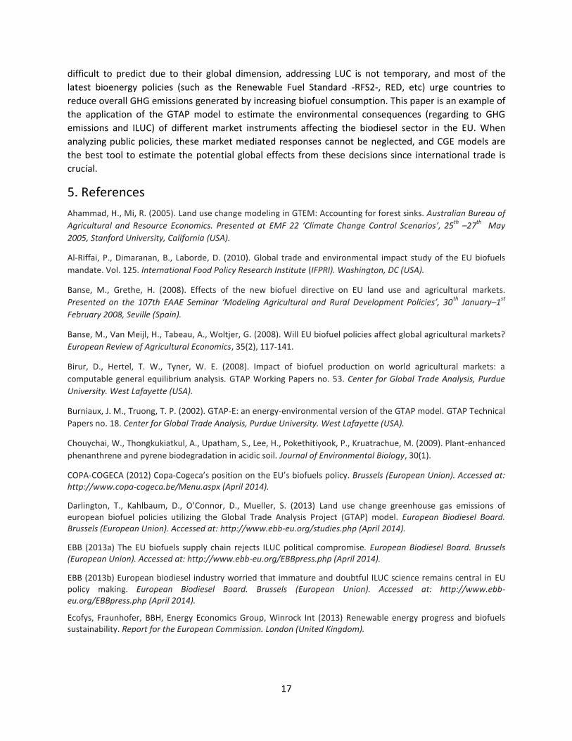
Figure B.1. Production nest in the GTAP-BIO-ADV model (Taheripour et al., 2011).

In the latest GTAP-BIO version, the biofuels composite is only disaggregated between Ethanol1 (from grains, mainly corn), Ethanol2 (from sugarcane) and Ethanol3 (from other feedstock: miscanthus, switchgrass and corn stover). The biodiesel composite is disaggregated between Biod_soy, Biod_rape, Biod_palm and Biod_oth (from other feedstock than soy, rape or palm). The version in the Figure B.1. was especially created to study the ILUC effects from the penetration of advanced biofuels (in this case, ethanol from non-food feedstock) into the US market. Besides ETA, there are two parameters, ETL1 and ETL2 (elasticity of transformation for land cover at bottom of supply tree and elasticity of transformation for crop land in supply tree) which distribute the sluggish endowment “cropland” across sectors.

22

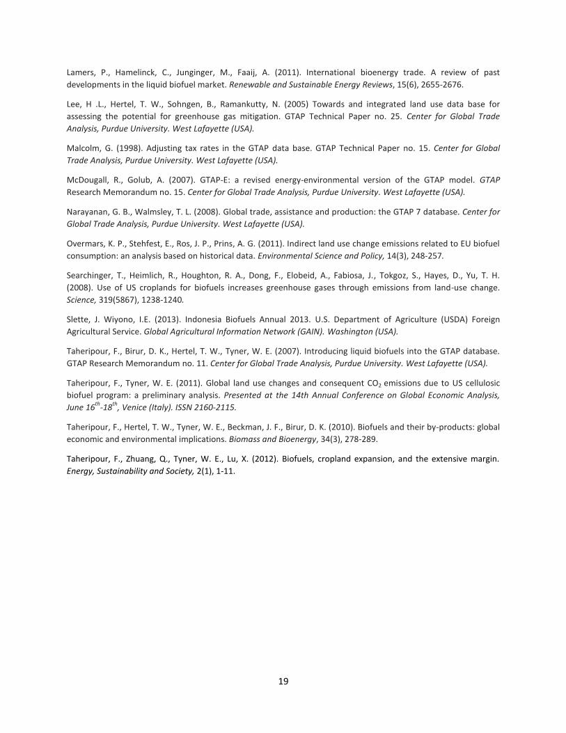
Annex C. Regions, industries and commodities included in the GTAP-BIO version.

Table C.1. Regions, industries and commodities considered for the GTAP-BIO version to analyze biofuel policies in depth.

Regions Industries Commodities

1 USA 1 Paddy_Rice 1 Paddy_Rice

2 EU27 2 Wheat 2 Wheat

3 Brazil 3 Sorghum 3 Sorghum

4 Canada 4 Oth_CoarseGrains 4 Oth_CoarseGrains

5 Japan 5 Soybeans 5 Soybeans

6 China-Hongkong 6 Palm 6 palmf

7 India 7 Rapeseed 7 Rapeseed

8 Central-Amer 8 Oth_Oilseeds 8 Oth_Oilseeds

9 S-Amer 9 Sugar_Crop 9 Sugar_Crop

10 E-Asia 10 Oth_Crops 10 Oth_Crops

11 Mala-Indo 11 Forestry 11 Forestry

12 SE-Asia 12 Dairy_Farms 12 Dairy_Farms

13 S-Asia 13 Ruminant 13 Ruminant

14 Russia 14 NonRuminant 14 NonRuminant

15 Oth-CEE 15 Proc_Dairy 15 Proc_Dairy

16 Oth-Europe 16 Proc_Rumiants 16 Proc_Rumiants

17 ME-Asia-N-Africa 17 Proc_NonRumiants 17 proc_NonRumiants

18 SS-Africa 18 Vol_Soy 18 Bev_Sug

19 Oceania 19 Vol_Palm 19 Proc_Rice

20 Vol_Rape 20 Proc_Food

21 Vol_Oth 21 Proc_Feed

22 Bev_Sug 22 Oth_PrimarySectors

23 Proc_Rice 23 Ethanol_sugarcane

24 Proc_Food 24 Biod_Soy

25 Proc_Feed 25 Biod_Palm

26 Oth_PrimarySectors 26 Biod_Rape

27 Ethanol_grains 27 Biod_Oth

28 Ethanol_sugarcane 28 Coal

29 Ethanol_Oth 29 Oil

30 Biod_Soy 30 Gas

31 Biod_Palm 31 Oil_Products

32 Biod_Rape 32 Electricity

33 Biod_Oth 33 Energy_Int_Ind

34 Coal 34 Oth_Ind_Services

35 Oil 35 NTrdServices

36 Gas 36 Pasturecrop

37 Oil_Products 37 Ethanol_grains

38 Electricity 38 DDGS

39 Energy_Int_Ind 39 Vol_Soy

40 Oth_Ind_Services 40 VOBPS

41 NTrdServices 41 Vol_Palm

42 Pasturecrop 42 VOBPP

43 Vol_Rape

44 VOBPR

45 Vol_Oth

46 VOBPO

47 Ethanol_Oth

48 DDGSS

23

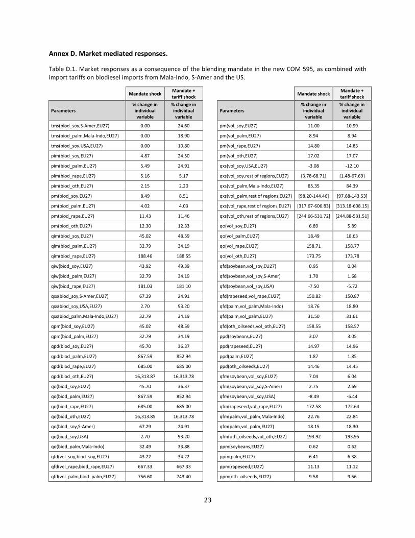
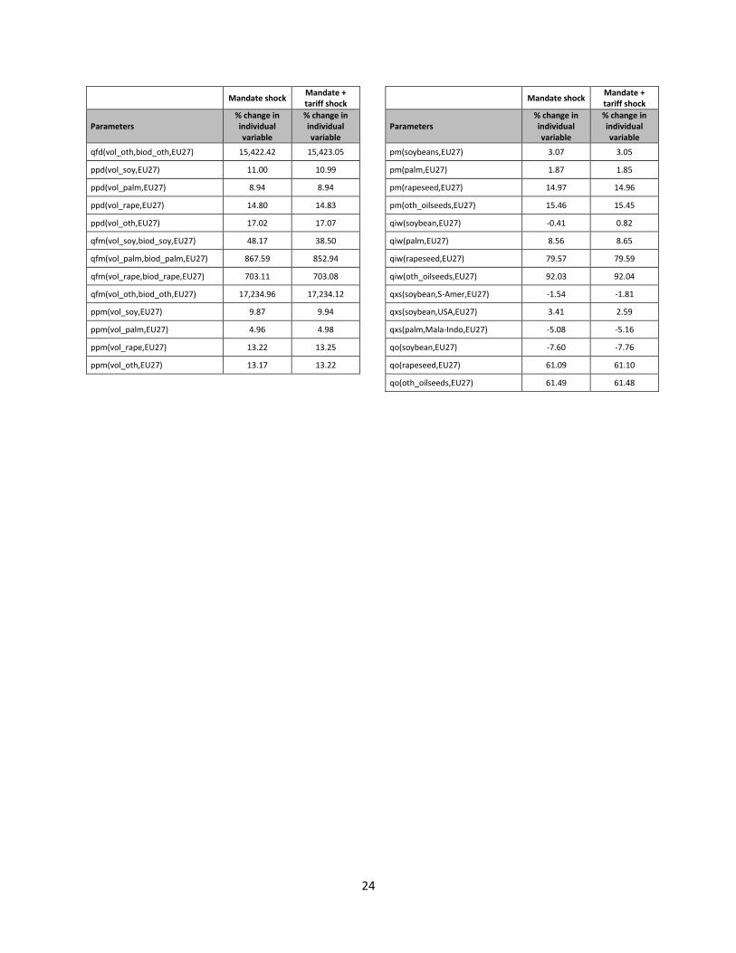
Annex D. Market mediated responses.

Table D.1. Market responses as a consequence of the blending mandate in the new COM 595, as combined with import tariffs on biodiesel imports from Mala-Indo, S-Amer and the US.

Mandate shock Mandate + tariff shock


Parameters % change in individual variable

% change in individual variable

Parameters



tms(biod_soy,S-Amer,EU27) 0.00 24.60

pm(vol_soy,EU27) 11.00 10.99

tms(biod_palm,Mala-Indo,EU27) 0.00 18.90

pm(vol_palm,EU27) 8.94 8.94

tms(biod_soy,USA,EU27) 0.00 10.80

pm(vol_rape,EU27) 14.80 14.83

pim(biod_soy,EU27) 4.87 24.50

pm(vol_oth,EU27) 17.02 17.07

pim(biod_palm,EU27) 5.49 24.91

qxs(vol_soy,USA,EU27) -3.08 -12.10

pim(biod_rape,EU27) 5.16 5.17

qxs(vol_soy,rest of regions,EU27) [3.78-68.71] [1.48-67.69]

pim(biod_oth,EU27) 2.15 2.20

qxs(vol_palm,Mala-Indo,EU27) 85.35 84.39

pm(biod_soy,EU27) 8.49 8.51

qxs(vol_palm,rest of regions,EU27) [98.20-144.46] [97.68-143.53]

pm(biod_palm,EU27) 4.02 4.03

qxs(vol_rape,rest of regions,EU27) [317.67-606.83] [313.18-608.15]

pm(biod_rape,EU27) 11.43 11.46

qxs(vol_oth,rest of regions,EU27) [244.66-531.72] [244.88-531.51]

pm(biod_oth,EU27) 12.30 12.33

qo(vol_soy,EU27) 6.89 5.89

qim(biod_soy,EU27) 45.02 48.59

qo(vol_palm,EU27) 18.49 18.63

qim(biod_palm,EU27) 32.79 34.19

qo(vol_rape,EU27) 158.71 158.77

qim(biod_rape,EU27) 188.46 188.55

qo(vol_oth,EU27) 173.75 173.78

qiw(biod_soy,EU27) 43.92 49.39

qfd(soybean,vol_soy,EU27) 0.95 0.04

qiw(biod_palm,EU27) 32.79 34.19

qfd(soybean,vol_soy,S-Amer) 1.70 1.68

qiw(biod_rape,EU27) 181.03 181.10

qfd(soybean,vol_soy,USA) -7.50 -5.72

qxs(biod_soy,S-Amer,EU27) 67.29 24.91

qfd(rapeseed,vol_rape,EU27) 150.82 150.87

qxs(biod_soy,USA,EU27) 2.70 93.20

qfd(palm,vol_palm,Mala-Indo) 18.76 18.80

qxs(biod_palm,Mala-Indo,EU27) 32.79 34.19

qfd(palm,vol_palm,EU27) 31.50 31.61

qpm(biod_soy,EU27) 45.02 48.59

qfd(oth_oilseeds,vol_oth,EU27) 158.55 158.57

qpm(biod_palm,EU27) 32.79 34.19

ppd(soybeans,EU27) 3.07 3.05

qpd(biod_soy,EU27) 45.70 36.37

ppd(rapeseed,EU27) 14.97 14.96

qpd(biod_palm,EU27) 867.59 852.94

ppd(palm,EU27) 1.87 1.85

qpd(biod_rape,EU27) 685.00 685.00

ppd(oth_oilseeds,EU27) 14.46 14.45

qpd(biod_oth,EU27) 16,313.87 16,313.78

qfm(soybean,vol_soy,EU27) 7.04 6.04

qo(biod_soy,EU27) 45.70 36.37

qfm(soybean,vol_soy,S-Amer) 2.75 2.69

qo(biod_palm,EU27) 867.59 852.94

qfm(soybean,vol_soy,USA) -8.49 -6.44

qo(biod_rape,EU27) 685.00 685.00

qfm(rapeseed,vol_rape,EU27) 172.58 172.64

qo(biod_oth,EU27) 16,313.85 16,313.78

qfm(palm,vol_palm,Mala-Indo) 22.76 22.84

qo(biod_soy,S-Amer) 67.29 24.91

qfm(palm,vol_palm,EU27) 18.15 18.30

qo(biod_soy,USA) 2.70 93.20

qfm(oth_oilseeds,vol_oth,EU27) 193.92 193.95

qo(biod_palm,Mala-Indo) 32.49 33.88

ppm(soybeans,EU27) 0.62 0.62

qfd(vol_soy,biod_soy,EU27) 43.22 34.22

ppm(palm,EU27) 6.41 6.38

qfd(vol_rape,biod_rape,EU27) 667.33 667.33

ppm(rapeseed,EU27) 11.13 11.12

qfd(vol_palm,biod_palm,EU27) 756.60 743.40

ppm(oth_oilseeds,EU27) 9.58 9.56

24



Parameters % change in individual variable


Parameters



qfd(vol_oth,biod_oth,EU27) 15,422.42 15,423.05

pm(soybeans,EU27) 3.07 3.05

ppd(vol_soy,EU27) 11.00 10.99

pm(palm,EU27) 1.87 1.85

ppd(vol_palm,EU27) 8.94 8.94

pm(rapeseed,EU27) 14.97 14.96

ppd(vol_rape,EU27) 14.80 14.83

pm(oth_oilseeds,EU27) 15.46 15.45

ppd(vol_oth,EU27) 17.02 17.07

qiw(soybean,EU27) -0.41 0.82

qfm(vol_soy,biod_soy,EU27) 48.17 38.50

qiw(palm,EU27) 8.56 8.65

qfm(vol_palm,biod_palm,EU27) 867.59 852.94

qiw(rapeseed,EU27) 79.57 79.59

qfm(vol_rape,biod_rape,EU27) 703.11 703.08

qiw(oth_oilseeds,EU27) 92.03 92.04

qfm(vol_oth,biod_oth,EU27) 17,234.96 17,234.12

qxs(soybean,S-Amer,EU27) -1.54 -1.81

ppm(vol_soy,EU27) 9.87 9.94

qxs(soybean,USA,EU27) 3.41 2.59

ppm(vol_palm,EU27) 4.96 4.98

qxs(palm,Mala-Indo,EU27) -5.08 -5.16

ppm(vol_rape,EU27) 13.22 13.25

qo(soybean,EU27) -7.60 -7.76

ppm(vol_oth,EU27) 13.17 13.22

qo(rapeseed,EU27) 61.09 61.10

qo(oth_oilseeds,EU27) 61.49 61.48

global land use change and greenhouse gas emissions … · global land use change and greenhouse...

Documents