global k-level crossing reduction - emis · 632 bachmaier, brandenburg, brunner, hub ner global...

Journal of Graph Algorithms and Applicationshttp://jgaa.info/ vol. 15, no. 5, pp. 631–659 (2011)

Global k-Level Crossing Reduction

Christian Bachmaier 1 Franz J. Brandenburg 1 WolfgangBrunner 1 Ferdinand Hubner 2

1University of Passau, 94030 Passau, Germany2Bedag Informatik AG, 3011 Bern, Switzerland

Abstract

Directed graphs are commonly drawn by a four phase framework in-troduced by Sugiyama et al. in 1981. The vertices are placed on parallelhorizontal levels. The edge routing between consecutive levels is com-puted by solving one-sided 2-level crossing minimization problems, whichare repeated in up and down sweeps over all levels. Crossing minimizationproblems are generally NP-hard.

We introduce a global crossing reduction, which at any particular timeconsiders all crossings between all levels. Our approach is based on the sift-ing technique. It yields an improvement of 5 – 10% in the number of cross-ings over the level-by-level one-sided 2-level crossing reduction heuristics.In addition, it avoids type 2 conflicts which are crossings between edgeswhose endpoints are dummy vertices. This helps straightening long edgesspanning many levels. Finally, the global crossing reduction approach candirectly be extended to cyclic, radial, and clustered level graphs achievingsimilar improvements. The running time is quadratic in the size of theinput graph, whereas the common level-by-level approaches are faster butoperate on larger graphs with many dummy vertices for long edges.

Submitted:April 2010

Reviewed:October 2010

Revised:November 2010

Accepted:April 2011

Final:May 2011

Published:October 2011

Article type:Regular paper

Communicated by:M. S. Rahman and S. Fujita

Supported by the Deutsche Forschungsgemeinschaft (DFG), grant Br835/15-1.

A preliminary version [3] was presented at the Workshop on Algorithms and Computation,

WALCOM 2010.

E-mail addresses: [email protected] (Christian Bachmaier)

[email protected] (Franz J. Brandenburg) [email protected]

(Wolfgang Brunner) [email protected] (Ferdinand Hubner)

mailto:[email protected]




632 Bachmaier, Brandenburg, Brunner, Hubner Global Crossing Reduction

1 Introduction

The four phase framework introduced by Sugiyama et al. [43] is the standardalgorithm for drawing directed graphs. It displays them in a hierarchical man-ner and operates in four phases: cycle removal, leveling, crossing reduction, andcoordinate assignment. First, it reverses appropriate edges to eliminate cycles.Then, it assigns vertices to levels, which are their y-coordinates, and introducesdummy vertices splitting long edges at their crossings with spanned levels. Thisresults in a proper k-level graph. In the third phase the vertices are permutedwithin the levels to reduce edge crossings. Finally, the x-coordinates are com-puted such that all vertices have integral coordinates and the drawing meetssome aesthetic criteria such as few bends per edge. Typical applications forsuch drawings are schedules, UML diagrams, and flow charts, where temporalor causal dependencies are modeled by directed edges and are expressed by aleft to right or a downward direction, see [14,31,43].

In this paper we focus on the crossing reduction phase, where the verticeson each level are rearranged to minimize the total number of crossings. Thecommon solution to this NP-hard k-level crossing minimization problem [25]is a reduction to the one-sided 2-level crossing minimization problem, which issolved repeatedly in several up and down sweeps [31, 43]. In a down sweep thevertices Vi−1 in the upper level are fixed and the vertices Vi in the lower level arereordered reducing the local number of edge crossings between the two levels. Inan up sweep the roles of the levels are switched. The one-sided 2-level crossingminimization problem is NP-hard [19], even for forests of 4-stars [36]. However,there are many heuristics for this problem [31]. Small instances can be solvedexactly by an ILP approach [30]. There are no reasonable approximations forthe k-level crossing minimization problem. The ratios from the one-sided 2-levelcrossing minimization problem [19,37] do not translate to the general problem.

An important feature of crossing reduction algorithms is the absence of type2 conflicts, which are crossings of two edges between dummy vertices. Amongothers, our favored fourth phase algorithm of Brandes and Kopf [10] assumesthe absence of type 2 conflicts. It aligns long edges vertically and so meets animportant aesthetic criterion [31] for nice hierarchical drawings with at mosttwo bends per edge.

The barycenter and the median heuristic [31] are two common 2-level cross-ing reductions. They place each vertex v ∈ Vi at the barycenter or medianposition of its predecessors in Vi−1. Then, Vi is sorted by these values. So theedges shall be short and induce few crossings. These techniques are simple, fast,and avoid type 2 conflicts, but they often leave too many crossings.

In 2-level algorithms the number of crossings between levels Vi and Vi+1

and thus the total number of crossings can increase while permuting Vi for the2-level crossing reduction between Vi−1 and Vi. So, such heuristics push thecrossings downwards or upwards until they are resolved at the extreme levels.An immediate extension is the centered 3-level crossing reduction. Here, Vi ispermuted while keeping the orders of Vi−1 and Vi+1 fixed and considering thecrossings above and below level i. However, this introduces type 2 conflicts.

JGAA, 15(5) 631–659 (2011) 633

1

2

3

6

6

1 2 3

8

4 5

96 7 10 11 12 13

14 15 16 17 18

(a) Optimal level-by-level order with 12 crossings

1

2

3

5

5

1 2 3

8

4 5

96 7 10 11 1213

14 15 16 17 18

(b) Optimal order with 10 crossings

Figure 1: Crossing reduction using an exact level-by-level sweep method hasbeen stuck in a local minimum

All these approaches suffer from a general problem: They have a local viewto the crossing minimization problem. So they tend to get stuck in a localoptimum. Bastert and Matuszewski claim [31] that the results of a level-by-levelsweep are far from optimum. “One can expect better results by considering alllevels simultaneously, but k-level crossing minimization is a very hard problem”[31, page 102]. After empirical tests of several one-sided 2-level approachesStallmann et al. [42, page 32] drew the conclusion that “the most pressing issuefrom a practical perspective is a generalization to k > 2 levels”. Our approachaddresses this gap. Fig. 1 shows an example, where even an optimal one-sided2-level crossing reduction gets stuck in a local minimum. In the left componentof Fig. 1(a) an optimal top-down sweep swaps vertices 8 and 9, which reducesthe number of crossings by two. However, the subsequent bottom-up sweep willundo this change. Since the right component is symmetric, the graph has 12crossings independently of the direction of the final sweep. Our algorithm solvesthis example with the optimal solution with 10 crossings as shown in Fig. 1(b).

Tutte’s algorithm [18] can be seen as a first approach with a global view,but it does not address crossings directly. Its quality concerning the number ofcrossings is open, as Eades and Sugiyama [18] state in Problem 8. Here, thepositions of the vertices on the extreme levels are fixed in any order. For thevertices in the other levels the x-coordinate is chosen as the weighted averageof the x-positions of all its neighbors. This is modeled by a sparse system oflinear equations.


Sifting is a modification of sorting by insertion and it has been used success-fully for vertex minimization in ordered binary decision diagrams [40]. Later ithas been adapted to the one-sided 2-level crossing reduction problem [34]. Theidea is to keep track of the number of crossings while in a sifting step a vertexv ∈ Vi is moved along a fixed order of the vertices in Vi. Finally, v is placedat its locally best position. The method is an extension of the greedy-switchheuristic [17], where v is swapped iteratively with its current successor. Wecall a single swap a sifting swap and the execution of a sifting step for everyvertex in Vi a sifting round. In general, sifting leaves fewer crossings than thesimple one-sided 2-level heuristics at the expense of a higher running time andpotential type 2 conflicts [31].

Matuszewski et al. [34] have extended sifting towards a more global view,which we call ordered k-level sifting to avoid confusion. There, the verticesare sorted by their degree and are first sifted in increasing order and then indecreasing order. For swapping two consecutive vertices v and w their incidentedges to and from neighbors on both adjacent levels are taken into account. Theheuristic does not sweep level-by-level but is still limited to a local view, sincelong edges are not treated as a whole. Our centered 3-level sifting does the samewith the vertices ordered level-by-level. Both algorithms yield similar results.Junger et al. [29] have developed an exact ILP approach for the NP-hard k-level crossing minimization, which can be used in practice for small graphs.Moreover, metaheuristics have been proposed in the literature, such as geneticalgorithms [32,45], tabu search [33], or windows optimization [22]. These general(stochastic) global search approaches usually compute good solutions with fewcrossings at the expense of high running times.

In this paper we propose a new and global crossing reduction technique.The algorithm yields better results than the common heuristics. It is directlyextendable to more general crossing reduction problems, avoids type 2 conflicts,and runs in quadratic time in the size of the graph. This distinguishes ourapproach from most 2-level approaches which extensively use dummy vertices,whose number is up to O(k · |E|) ⊆ O(|V |3). Note that the edge bundlingtechnique of Eiglsperger et al. [21] groups dummy vertices horizontally in eachlevel. This improves the running time of the sweeping barycenter and medianheuristics to be independent of the number of dummy vertices. However, theirapproach cannot be used for more advanced heuristics like sifting.

Recently, Chimani et al. [11, 12] presented an advanced approach based onupward planarization which combines the leveling and the crossing reductionphases of the hierarchical framework. Generally, from an algorithm and soft-ware engineering perspective the subdivision of a complicated problem into dis-joint phases as done in the hierarchical framework makes sense. However, forobtaining global optima the phases cannot be treated independently, as is donetraditionally and also in this paper. For example, the number of crossingsclearly depends on the leveling. For a competitive extension of global siftingwhich performs leveling and crossing reduction simultaneously see [7].

The remainder of the paper is organized as follows: After introducing somenotation and previous results in the next section, we present our new crossing

JGAA, 15(5) 631–659 (2011) 635

reduction approach and analyze its complexity in Sect. 3. Then, in Sect. 4,we show benchmarks which empirically compare our algorithm with establishedstrategies. Afterwards, we present some applications of the block concept onrelated crossing optimization and reduction methods in Sect. 5. Finally, wesummarize the results and discuss some open problems in Sect. 6.

2 Preliminaries

We suppose that a directed graph without self-loops has passed the cycle removaland leveling phases of the four phase framework. The outcome is a k-level graphG = (V,E, φ), where φ : V → {1, 2, . . . , k} is a surjective level assignment of thevertices with φ(u) < φ(v) for each edge (u, v) ∈ E. For an edge e = (u, v) ∈ Ewe define its length as span(e) := φ(v)−φ(u). An edge e is short if span(e) = 1and long otherwise. A graph is proper if all edges are short. Each level graphcan be made proper by adding span(e)−1 dummy vertices for each edge e whichsplit e in span(e) many short edges. Let G′ = (V ′, E′, φ′) denote the properversion of G. As in [10] short edges are called segments of e. The first andthe last segments of an edge are the outer segments and the others the innersegments. Inner segments connect two dummy vertices.

Consider the proper level graph G′. For a vertex v we denote the set ofneighbors from incoming and outgoing segments by N−(v) := {u ∈ V ′ | (u, v) ∈E′ } and N+(v) := {w ∈ V ′ | (v, w) ∈ E′ }, respectively. G′ is ordered if thevertices in each level as well as the sets N−(·) and N+(·) are ordered from leftto right. Each proper level graph can be made ordered by choosing an arbitraryorder for each level. This induces an order of the sets N−(·) and N+(·). Letdeg−(v) := |N−(v)| and deg+(v) := |N+(v)| denote the indegree and outdegreeof a vertex v and set deg(v) := deg−(v) + deg+(v). In an ordered level graphtwo segments are in conflict if they cross or share a vertex. Conflicts are of type0, 1, or 2 if they are induced by 0, 1, or 2 inner segments, respectively.

Next, we define blocks, which prevent dealing with dummy vertices. Thus,the running time of our algorithm is measured in the size of the input graph andis independent of the number of dummy vertices. A block is a single vertex of Vor a maximum connected subgraph of dummy vertices, i. e., the inner segmentsof a long edge. The blocks represent the vertices of a graph related to G′, wherethe edges are the outer segments. We will always denote (dummy) verticesby lower case letters and blocks by upper case letters. For a block A definex = upper(A) (y = lower(A)) to be the unique vertex x in A (y in A) with noincoming (outgoing) segments in A. x and y always exist but may coincide.

LetN−(A) := N−(upper(A)), N+(A) := N+(lower(A)), deg(A) := |N−(A)|+|N+(A)|, and let levels(A) be the set of level numbers which contain (dummy)vertices of A. With block(v) we denote the block of the vertex v ∈ V ′. Let Bbe an arbitrarily ordered list of all blocks and let π : B → {0, . . . , |B| − 1} as-sign each block its current position in this order. We use the binary relation ≺with A ≺ B ⇔ π(A) < π(B) for comparing blocks A,B ∈ B according to theirpositions π.


2.1 One-Sided 2-Level Sifting

In a sifting step the locally best position for a vertex is sought. Therefore,all positions in its level are tested sequentially, where the cost criterion is thenumber of crossings. For its computation we adapt the idea of Baur and Brandes[8], which was introduced for circular crossing reduction.

Consider a sifting step for a 2-level graph G = (V1.∪V2, E, φ) with the vertex

orders πi : Vi → {1, . . . , |Vi|} in levels i ∈ {1, 2} with π1 fixed. To determine alocally optimal position of a vertex v ∈ V2 it is sufficient to record the change inthe number of crossings while swapping v with its current consecutive successorw ∈ V2. For this, only edges incident to v or w must be considered. After aswap exactly those pairs of these edges cross which did not cross before. Allother crossings remain unchanged. Let χ(π2) be the number of crossings of anorder (π1, π2) of G and χπ2

(e, f) ∈ {0, 1} be the number of crossings betweentwo edges e, f ∈ E. Then, we obtain Lemma 1 by a direct adaption from [8],which formalizes the change in the number of crossings per swap. At the endof one step v is placed where the intermediary crossing counts reached theirminimum.

Lemma 1 (Bauer, Brandes) Let v, w ∈ V2 with π2(v) = π2(w) − 1 be con-secutive vertices of a 2-level graph G = (V1

.∪ V2, E, φ) in an order (π1, π2) and

let (π1, π′2) be the order with their positions swapped, then

χ(π′2) = χ(π2)− cπ2(v, w) + cπ′2(v, w),

where cπ2(v, w) =

∑u∈N−(v)

∑x∈N−(w)

χπ2((u, v), (x,w)) .

3 Global Sifting

A major drawback of the established crossing reduction algorithms is their localview. We present a new approach using ideas from [10] and [21], which avoidstype 2 conflicts. Eiglsperger et al. [21] have used a data structure similar to ourblocks and avoid type 2 conflicts. However, for crossing reduction they proceedlevel-by-level in the traditional fashion. This improves only the running timebut not the quality of the result. We treat all dummy vertices of an edge andeach original vertex as a block and find the locally best position for the wholeblock in one sifting step. This eliminates a problem of 2-level approaches whichlack this global view on crossings of long edges. In the initialization the list ofblocks B is sorted arbitrarily and each block A receives its position π(A) in B(line 1 in Algorithm 1). At any time during the execution of the algorithm weinterpret π(A) as an x-coordinate of each vertex v in the block A and φ(v) asits y-coordinate. This results in a drawing respecting the current order of B.All vertices of a block get the same x-coordinate. Hence, the order is type 2conflict free. These are important properties of Algorithm 1.

The main part of the algorithm is the sifting step (line 4). There, all positionsfor a block A are tested and A is moved to the position with the fewest crossings.

JGAA, 15(5) 631–659 (2011) 637

This is done for each block A ∈ B (line 3) and repeated a certain number oftimes (line 2). Alternatively, one may repeat until the improvement is below agiven threshold. Our experiments have shown that ten rounds suffice to reachsuch a situation. Finally, each vertex is set to the position of its block (line 5),the vertices in each level are sorted according to these positions (line 6). Finally,the graph is returned (line 7).

Algorithm 1: GLOBAL-SIFTING

Input: Proper k-level graph G′ = (V ′, E′, φ′), number ρ of sifting roundsOutput: Graph G′ with vertices ordered by values π(v) for each v ∈ V ′

1 create list B of all blocks in G′

2 for 1 ≤ i ≤ ρ do3 foreach A ∈ B do4 B ← SIFTING-STEP(G′, B, A)

5 foreach v ∈ V ′ do π(v)← π(block(v))6 sort vertices in each level according to π7 return G′

3.1 Building the Block List

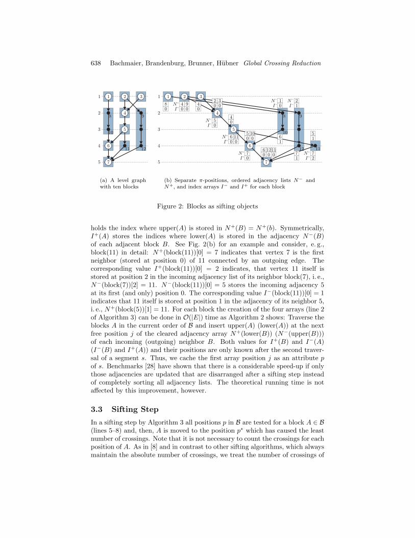
The graph is partitioned into blocks. Each block A gets an arbitrary but uniqueposition π(A) in the block list B. As an example consider Fig. 2(a). The inputgraph with 7 vertices has 6 dummy vertices, which are drawn as black circles.The dummy vertices are combined into 3 blocks and each original vertex formsits own block. The 10 resulting blocks are shown in Fig. 2(b) with an arbitraryorder π.

If a given order (without type 2 conflicts) shall only be improved by globalsifting in a postprocessing step, a straightforward initialization strategy is totopologically sort the blocks according to the order in the levels from left toright in O(|E′|). Our experiments have shown that a good initial order of theblocks leads to better results. However, these can also be achieved by one ortwo additional sifting rounds.

3.2 Initialization of a Sifting Step

To improve the performance of one sifting step [8] it is necessary to keep the adja-cency lists N−(A) and N+(A) of each block A ∈ B sorted according to ascendingpositions of the neighboring blocks in B. We store them in arrays for randomaccess. Additionally, we store two index arrays I−(A) = I−(upper(A)) andI+(A) = I+(lower(A)) of lengths |I−(A)| := |N−(A)| and |I+(A)| := |N+(A)|,respectively. As an inverted file I−(A) stores the indices where upper(A) isstored in each adjacent block B’s adjacency array N+(B). More precisely, letb = N−(A)[i] be a neighbor of upper(A) with B = block(b). Then, I−(A)[i]


1

2

3

4

5

1

7

2 3

4

5

6

8 9

10

11 12

(a) A level graphwith ten blocks

1

2

3

4

5

1

7

2

8

0

5

0

2

0 0

34

0

9

0

4

0

N+

I+

6

0

11

0

4

0

2

1

N

I

1

0

6

1

6

0

12

0

11

0 7

1

5

1

7

2

7

0

5

0

10

0

3

4

5

6

N+

I+

N+

I+

N+

I+

N+

I+

N

I

10

12 11

8 9

(b) Separate π-positions, ordered adjacency lists N− andN+, and index arrays I− and I+ for each block

Figure 2: Blocks as sifting objects

holds the index where upper(A) is stored in N+(B) = N+(b). Symmetrically,I+(A) stores the indices where lower(A) is stored in the adjacency N−(B)of each adjacent block B. See Fig. 2(b) for an example and consider, e. g.,block(11) in detail: N+(block(11))[0] = 7 indicates that vertex 7 is the firstneighbor (stored at position 0) of 11 connected by an outgoing edge. Thecorresponding value I+(block(11))[0] = 2 indicates, that vertex 11 itself isstored at position 2 in the incoming adjacency list of its neighbor block(7), i. e.,N−(block(7))[2] = 11. N−(block(11))[0] = 5 stores the incoming adjacency 5at its first (and only) position 0. The corresponding value I−(block(11))[0] = 1indicates that 11 itself is stored at position 1 in the adjacency of its neighbor 5,i. e., N+(block(5))[1] = 11. For each block the creation of the four arrays (line 2of Algorithm 3) can be done in O(|E|) time as Algorithm 2 shows: Traverse theblocks A in the current order of B and insert upper(A) (lower(A)) at the nextfree position j of the cleared adjacency array N+(lower(B)) (N−(upper(B)))of each incoming (outgoing) neighbor B. Both values for I+(B) and I−(A)(I−(B) and I+(A)) and their positions are only known after the second traver-sal of a segment s. Thus, we cache the first array position j as an attribute pof s. Benchmarks [28] have shown that there is a considerable speed-up if onlythose adjacencies are updated that are disarranged after a sifting step insteadof completely sorting all adjacency lists. The theoretical running time is notaffected by this improvement, however.

3.3 Sifting Step

In a sifting step by Algorithm 3 all positions p in B are tested for a block A ∈ B(lines 5–8) and, then, A is moved to the position p∗ which has caused the leastnumber of crossings. Note that it is not necessary to count the crossings for eachposition of A. As in [8] and in contrast to other sifting algorithms, which alwaysmaintain the absolute number of crossings, we treat the number of crossings of

JGAA, 15(5) 631–659 (2011) 639

Algorithm 2: SORT-ADJACENCIES

Input: Proper k-level graph G′ = (V ′, E′, φ′), ordered list B of blocks inG′

Output: Ordered sets N ·(A) and I ·(A) for each block A ∈ B1 for i← 0 to |B| − 1 do2 π(B[i])← i3 clear the arrays N−(B[i]), N+(B[i]), I−(B[i]), and I+(B[i])

4 foreach A ∈ B do5 foreach s ∈ { (u, v) ∈ E′ | v = upper(A) } do6 insert v at the next free position j of N+(u)7 if π(A) < π(block(u)) then p[s]← j // first traversal of s8 else I+(u)[j]← p[s]; I−(v)[p[s]]← j // second traversal of s

9 foreach s ∈ { (w, x) ∈ E′ | w = lower(A) } do10 insert w at the next free position j of N−(x)11 if π(A) < π(block(x)) then p[s]← j // first traversal of s12 else I−(x)[j]← p[s]; I+(w)[p[s]]← j // second traversal of s

A as χ = 0 when A is placed to the first position. Thereafter, we only computethe change in the number of crossings when A is iteratively swapped with itsright neighbor (line 6).

Algorithm 3: SIFTING-STEP

Input: Proper k-level graph G′ = (V ′, E′, φ′),ordered list B of blocks in G′, block A ∈ B to sift

Output: Updated order of B1 B′ ← A ≺ B[0] ≺ · · · ≺ B[|B| − 1] // new order B′ with A put to front2 SORT-ADJACENCIES(G′, B′)3 χ← 0; χ∗ ← 0 // current and best number of crossings4 p∗ ← 0 // best block position5 for p← 1 to |B′| − 1 do6 χ← χ+ SIFTING-SWAP(A,B′[p])7 if χ < χ∗ then8 χ∗ ← χ; p∗ ← p

9 return B′[1] ≺ · · · ≺ B′[p∗] ≺ A ≺ B′[p∗ + 1] ≺ · · · ≺ B′[|B′| − 1]

3.4 Sifting Swap

The sifting swap computes the change in the number of crossings when a blockA is swapped with its right successor B in B. In contrast to one-sided crossingreduction, our global approach takes the whole neighborhood of both blocks


into account when it computes the change in the number of crossings. Lemma 2states which segments are involved.

Lemma 2 Let B be the block list in the current order. Let B ∈ B be thesuccessor of A ∈ B. If swapping A and B changes the crossings between twosegments, then one of them is an incident outer segment of A or B and the othersegment is an incident outer segment of the same kind (incoming or outgoing)or an inner segment of the other block.

Proof: Note that only segments between the same levels can cross. As no type2 conflicts occur, at least one of the segments of a crossing has to be an outersegment. Let (a, b) and (c, d) be two segments between the same levels witha 6= c and b 6= d. If the two segments cross after swapping A and B and theydid not cross before (or vice versa) either a and c or b and d were swapped.Therefore, one of the segments is adjacent to A or is a part of A and the otheris adjacent to B or is a part of B. If b and d were swapped and thus a and cwere not, φ(b) = φ(d) is the upper level of A or B and thus one of the crossingsegments is an incoming outer segment of A or B. The other segment is eitheran incoming outer segment or an inner segment of the other block. Note that itcannot be an outgoing outer segment of this block because then neither a andc nor b and d would have been swapped. The other case of swapping a and cinstead of b and d is symmetric. Then, the second segment is either an outgoingouter segment or an inner segment of the other block. �

The following fact is easily seen and the resulting changes in the number ofcrossings are obvious.

Fact 1 Let B be the block list in the current order. Let B ∈ B be the successorof A ∈ B. Let i and j be the two levels framing the incoming outer segmentsof A (the other three cases are symmetric). If there is a segment (u, v) betweeni and j which is either an incoming outer segment of B or an inner segmentof B, then the incoming segments of A starting at a block left of block(u) cross(u, v) only after the swap of A and B, the segments starting at block(u) nevercross (u, v), and the segments starting right of block(u) cross (u, v) only beforethe swap. There are no other changes among the crossings due to Lemma 2.

For an illustration consider Fig. 3. The incoming segment (u, v) of blockB starts at block C. Thus, all incoming segments of A starting at a blockleft of C, namely (1, 2) and (6, 2), cross (u, v) only after the swap of A and B.The segment connecting blocks C and A, i. e., (u, 2), never crosses (u, v) and theincoming segments of A starting right of block C, namely (7, 2), cross (u, v) onlybefore the swap. The outgoing segment (2, 3) of A crosses the inner segment(v, 8) of B only after the swap.

Algorithm 4 shows the details of a sifting swap. First, the levels at which(significant) swaps occur and the direction of the segments changing their cross-ings are found (lines 2–6). For each entry (l, d) of the set L the two vertices aand b of A and B on level l are retrieved.

JGAA, 15(5) 631–659 (2011) 641

i

jv

A

B

1

3

5

6 7

8

C4

u

2

(a) Current block order

i

j

A

B

1

C

3

u

2v

5

6 7

8

4

(b) Blocks A and B swapped

Figure 3: Changes in crossings for a swap

Algorithm 4: SIFTING-SWAP

Input: Consecutive blocks A,B in the ordered blocklist BOutput: Change in crossing count

1 begin2 L ← ∅; ∆← 0 // L is a set and, thus, duplicate free3 if φ(upper(A)) ∈ levels(B) then L ← L ∪ {(φ(upper(A),−)}4 if φ(lower(A)) ∈ levels(B) then L ← L ∪ {(φ(lower(A),+)}5 if φ(upper(B)) ∈ levels(A) then L ← L ∪ {(φ(upper(B),−)}6 if φ(lower(B)) ∈ levels(A) then L ← L ∪ {(φ(lower(B),+)}7 foreach (l, d) ∈ L do8 let a in A and b in B be the vertices with φ(a) = φ(b) = l

9 ∆← ∆ + USWAP(a, b,Nd(a), Nd(b))

10 UPDATE-ADJACENCY(a, b,Nd(a), Id(a), Nd(b), Id(b))

11 swap positions of A and B in B; π(A)← π(A) + 1; π(B)← π(B)− 112 return ∆


When swapping A and B only a and b are swapped in their level and no orderchanges in the level of their neighbors Nd(a) and Nd(b). Thus, the computationof the change in the number of crossings can be done as in [8] and is describedin Algorithm 5: The neighbors are traversed from left to right. If a neighborof a is found (lines 5 and 6), its segment will cross all remaining s− j incidentsegments of b after the swap. If a neighbor of b is found (lines 7 and 8), itssegment has crossed all remaining r− i incident segments of a before the swap.Common neighbors present both cases at the same time (line 9).

Algorithm 5: USWAP

Input: Consecutive vertices a, b ∈ V , Nd(a), Nd(b) ∈ VOutput: Change in crossing count

1 let x0 ≺ · · · ≺ xr−1 ∈ Nd(a) be the neighbors of a in direction d

2 let y0 ≺ · · · ≺ ys−1 ∈ Nd(b) be the neighbors of b in direction d3 c← 0; i← 0; j ← 04 while i < r and j < s do5 if π(block(xi)) < π(block(yj)) then6 c← c+ (s− j); i← i+ 17 else if π(block(xi)) > π(block(yj)) then8 c← c− (r − i); j ← j + 19 else c← c+ (s− j)− (r − i); i← i+ 1; j ← j + 1

10 return c

An update of the adjacency after a swap (line 10) is necessary if a and bhave common neighbors. Algorithm 6 shows how this can be done in over-all O(deg(A) + deg(B)) time similarly to the crossing counting function Algo-rithm 5.

3.5 Time Complexity

Lemma 3 Let G = (V,E, φ) be a level graph. Then,∑B∈B deg(B) ≤ 4 · |E|.

Proof: Every edge e ∈ E contains at most two outer segments. Every outersegment increases the degree of its two incident blocks by one each. �

Theorem 1 One round of global sifting (Algorithm 1) has a time complexity ofO(|E|2) for a non-necessarily proper level graph G = (V,E, φ).

Proof: Let B be the blocks of G. Swapping two blocks A,B ∈ B needsO(deg(A) + deg(B)) time. Initializing a sifting step takes O(

∑B∈B deg(B)) =

O(|E|) time. A sifting step of a blockA needsO(∑B∈B\{A}(deg(A)+deg(B))) =

O(|E| · deg(A)) time. Thus, a sifting round for each block A ∈ B has time com-plexity O(

∑A∈B(|E| · deg(A)) = O(|E|2). Since |V ′| ≤ k · |E| ∈ O(|E|2) (no

empty levels), traversing all (dummy) vertices in pre- and postprocessing hasno effect on the worst case time complexity. �

JGAA, 15(5) 631–659 (2011) 643

Algorithm 6: UPDATE-ADJACENCIES

Input: Vertices a, b ∈ V ′, Nd(a), Id(a), Nd(b), Id(b)Output: Updated adjacencies of a and b and all common neighbors

1 let x0 ≺ · · · ≺ xr−1 ∈ Nd(a) be the neighbors of a in direction d

2 let y0 ≺ · · · ≺ ys−1 ∈ Nd(b) be the neighbors of b in direction d3 i← 0; j ← 04 while i < r and j < s do5 if π(block(xi)) < π(block(yj)) then i← i+ 16 else if π(block(xi)) > π(block(yj)) then j ← j + 17 else8 z ← xi // = yj9 swap entries at pos. Id(a)[i] and Id(b)[j] in N−d(z) and in I−d(z)

10 Id(a)[i]← Id(a)[i] + 1; Id(b)[j]← Id(b)[j]− 111 i← i+ 1; j ← j + 1

4 Experimental Results

For the sake of completeness we have extended the barycenter and median cross-ing reduction strategies to blocks as well. We iteratively take the π-positionsof the blocks in B and compute for each block the barycenter or median of itsadjacent blocks, respectively. Then, we sort B according to these values. Thefollowing benchmarks show that both are fast, however, they are not compet-itive with global sifting in the number of obtained crossings. One round ofglobal barycenter or global median has a time complexity of O(|E| log |E|) or ofO(|E|), respectively.

We have compared the practical performance of four level-by-level and fourglobal crossing reduction algorithms implemented in our graph tool Gravisto[5]: iterative one-sided 2-level barycenter (B), median (M), sifting (S), iterativecentered 3-level sifting (3S), global barycenter (GB), global median (GM), globalsifting (GS), and ordered k-level sifting (OS). For each of the level-by-levelalgorithms we run ten top-down and bottom-up sweeps and for each of the globalheuristics we performed ten rounds. We have tested 910 random graphs. Foreach graph size from 1,000 to 10,000 vertices in steps of 100 we have generated

ten arbitrary graphs with an aspect ratio of the golden rectangle 1+√5

2 , i. e., themaximum number of (dummy) vertices per level is about 1.6 times the number oflevels. The density of the proper edges is twice the number of vertices includinga proportion of 75% dummy vertices. Hence, there are five times as many (long)edges as non-dummy vertices. To aggregate random initializations we appliedeach algorithm twice to every concrete graph instance. All benchmarks wererun on a 2.83 GHz XEON workstation under Solaris and the Java 6.0 platformof Oracle Corp.


0

2

4

6

8

10

2000 4000 6000 8000 10000

Ru

nn

ing

tim

ein

seco

nd

s

Graph size |V ′| (75% dummy vertices and |E′| = 2 · |V ′|, i. e., |E| = 5 · |V |)

GSOS3SS

MB

GMGB

Figure 4: Benchmark: running times

We compare the different running times in Fig. 4. Although global siftingis the slowest among them, it is feasible in practice. Clearly, its performanceon real-world graphs is not as dire as the worst case O(|E|2) time complexityindicates at first glance.

Fig. 5 shows the quality of the heuristics in the number of crossings of theresulting embeddings. The results of global sifting are about 5 to 10% betterthan the ones of the established algorithms. In addition, type 2 conflicts areavoided, which are quite high for the sifting algorithms as Fig. 6 indicates, andwhich have an impact on the edge routing in the final phase of the four phaseframework. Both benefits justify the higher running time.

Fig. 7 depicts that the traditional approaches have a constant running timeon graphs with the same size but ascending proportions of dummy vertices.For global sifting the running times become better with more dummy vertices.Then, there are more long edges whose inner segments are treated as a whole.This reflects that the time complexity O(|E|2) depends only on the number ofedges |E| and not on the number of segments |E′| of the proper graph.

In Fig. 8 we compare the results of the heuristics with the exact solution.For a practically solvable ILP of the exact algorithm which will be describedin Sect. 5.1, the graphs must be small with |V ′| ≤ 35. Although permitted,the optimum solutions do not contain any type 2 conflicts. The graphs seemto be simply too small for that. Since we have a proportion of 30% dummyvertices, the graphs are rather sparse. This may be the reason why barycenterhere outperforms two sifting algorithms. Global sifting is in parts 25% closer tothe optimum as all other tested methods. Fig. 5 supports the statement in [31]that in general sifting is qualitatively the better choice.

Fig. 9 presents the influence of the number of sweeps or rounds in the num-ber of crossings. Again, global barycenter and median perform very poorly.Interestingly, the simple barycenter, median, and sifting heuristics seem to needonly one sweep. The remaining heuristics (OS, 3S, GS) improve their results

JGAA, 15(5) 631–659 (2011) 645

0.300.350.400.450.500.550.600.650.700.75

2000 4000 6000 8000 10000

Cro

ssin

gsaf

ter

vs.

bef

ore


GMGB

MBS

3SOSGS

Figure 5: Benchmark: number of crossings after vs. before applying the crossingreduction

1

10

100

1000

10000

100000

2000 4000 6000 8000 10000

Typ

e2

con

flic

ts


3SOS

S

Figure 6: Benchmark: number of type 2 conflicts


0

0.5

1

1.5

2

2.5

0 0.1 0.2 0.3 0.4 0.5 0.6 0.7 0.8

Ru

nn

ing

tim

ein

seco

nd

s

Dummy vs. all vertices (|V ′| = 2500, |E′| = 5000)

GS3S

OSS

MB

GMGB

Figure 7: Benchmark: running times with different proportions of dummy ver-tices

11.21.41.61.8

22.22.42.62.8

3

10 15 20 25 30 35

Heu

rist

icvs.

exac

t

Graph size |V ′| (30% dummy vertices and |E′| = 1.25 · |V ′|, i. e.,|E| ≈ 1.36 · |V |)

MS

3SB

OSGS

Figure 8: Benchmark: number of crossings compared to optimal solutions

JGAA, 15(5) 631–659 (2011) 647

0.3

0.4

0.5

0.6

0.7

0.8

0.9

5 10 15 20 25 30 35 40 45 50

Cro

ssin

gsaft

ervs.

bef

ore

Number of sweeps or rounds (|V ′| = 2500, |E′| = 5000, 75% dummy vertices)

GMGB

BS

M3S

OSGS

Figure 9: Benchmark: number of sweeps or rounds on graphs with 2500(dummy) vertices

over the first five sweeps or rounds. As tests with different sizes of graphs gavesimilar diagrams, we conclude that at least ten rounds of global sifting shouldbe sufficient in practice.

We additionally have tested the algorithms on the widely used Rome graphs[16] library in Fig. 10. The set contains 11528 instances with 10–100 verticesand 9–158 edges. Although these graphs are originally undirected, we inter-pret them as directed by artificially directing the edges according to the vertexorder given in the input files, see, e. g., [12, 20]. Furthermore, we have testedthe AT&T graphs [38], see Fig. 11. This benchmark set consists of 1155 di-rected acyclic graphs with 10–96 vertices and 10–99 edges collected by StephenNorth. Since these graphs are rather inhomogeneous in the number of vertices,we follow [15] and group the graphs by the number of edges to improve the read-ability of the diagram. For both benchmarks we have done the leveling withthe Coffman/Graham algorithm [13], where we allowed a maximum number of√|V | non-dummy vertices on the levels. Since the graphs are rather sparse

and contain many chains, we have marked all vertices with degree 2 as dummyvertices in a preprocessing step. This helps to build reasonable blocks for globalsifting. In both benchmarks global sifting gives the best results of all algorithmsguaranteeing no type 2 conflicts.

In a nutshell, classic sifting is fast, leaves few type 2 conflicts, but manycrossings. Centered 3-level sifting is fast, leaves few crossings, but many type 2conflicts. Global sifting leaves even fewer crossings without any type 2 conflicts,but has the highest running time which is still feasible in practice. The mea-surements reflect that the running time of global sifting is independent of thenumber of dummy vertices. This parallels the edge bundling technique in [21].Global sifting is a good choice for the trade-off between time and quality.


0

100

200

300

400

500

600

10 20 30 40 50 60 70 80 90 100

Nu

mb

erof

cross

ings

Graph size |V |

GBGM

MSB

GS3S

OS

Figure 10: Benchmark: number of crossings in the Rome graphs

0

50

100

150

200

250

10–19

20–29

30–39

40–49

50–59

60–69

70–79

80–89

90–99

Nu

mb

erof

cross

ings

Number of edges |E|

GBGM

SMB

GS3S

OS

Figure 11: Benchmark: number of crossings in the AT&T graphs

JGAA, 15(5) 631–659 (2011) 649

5 Applications of the Global Crossing Reduc-tion

In several related algorithms blocks for long edges can be used to improve theirperformance and the quality of the resulting drawings by avoiding type 2 con-flicts.

5.1 Optimal Crossing Reduction Using an ILP

Junger et al. [29] introduced an ILP formulation for the exact crossing mini-mization problem of k-level graphs. There, type 2 conflicts can be excludedby adding additional constraints, which after a simplification result in a similarILP as in our approach. However, using variables for pairs of overlapping blockswith common levels gives a more direct formulation which naturally excludestype 2 conflicts. It uses fewer variables by avoiding the use of dummy verticesfor computing a solution of the ILP. However, for forming the equations thegraph must be proper.

Our ILP is built as follows: We start with an arbitrary but fixed order ofthe list of blocks B. For any two blocks A and B with π(A) < π(B) and acommon level we define a boolean variable xAB . The value xAB = 1 denotesthat A is left of B and xAB = 0 that B is left of A in the final embedding. Foreach triple of blocks A, B, and C with π(A) < π(B) < π(C) with at least onecommon level, i. e., levels(A) ∩ levels(B) ∩ levels(C) 6= ∅, we add the condition0 ≤ xAB + xBC − xAC ≤ 1 to exclude cyclic dependencies within a level.

Let s1 = (a, b) and s2 = (c, d) be segments between the same levels such thatat least one of them is an outer segment. Let A = block(a), B = block(b), C =block(c), and D = block(d). Note that A = B or C = D holds if s1 or s2 isan inner segment, respectively. W. l. o. g. let π(A) < π(C). We add a booleancrossing variable cABCD which indicates whether or not s1 and s2 cross. Ifπ(B) < π(D), we add the constraint −cABCD ≤ xBD−xAC ≤ cABCD, otherwisewe add 1 − cABCD ≤ xDB − xAC ≤ 1 + cABCD. The objective function is tominimize the sum of the values of all crossing variables. See (1) for the completeILP formulation for a proper k-level graph G′ = (V ′, E′, φ′) of G with I ⊂ E′

denoting the set of inner segments. Informally speaking, each element of the setC denotes the up to four incident blocks of each pair of edges which may cross.

χopt = min∑

(A,B,C,D)∈C

cABCD

C = { (A,B,C,D) ∈ B4 | ∃(a, b), (c, d) ∈ E′ :(a, b) 6∈ I ∨ (c, d) 6∈ I,φ(b) = φ(d),A = block(a), B = block(b),C = block(c), D = block(d),π(A) < π(C) }

(1)


subject to

−cABCD ≤ xBD − xAC ≤ cABCD for (A,B,C,D) ∈ C,π(B) < π(D)

1− cABCD ≤ xDB − xAC≤ 1 + cABCD for (A,B,C,D) ∈ C,

π(B) > π(D)0 ≤ xAB + xBC − xAC ≤ 1 for A,B,C ∈ B,

π(A) < π(B) < π(C),levels(A) ∩ levels(B)∩ levels(C) 6= ∅

xAB ∈ {0, 1} for A,B ∈ B,π(A) < π(B)

cABCD ∈ {0, 1} for (A,B,C,D) ∈ C

According to our experiments, this approach is usable for graphs with up toforty vertices without further polyhedral studies. This is comparable with theoriginal approach in [29].

5.2 Level Planarity Testing Using the Vertex ExchangeGraph

Harrigan and Healy [27] introduced vertex exchange graphs as a data structurefor a simple level planarity test in O(|V ′|2) time, where V ′ ⊇ V is the set ofall vertices including dummy vertices. Using our blocks, it is straightforwardto improve the running time of the test from O(|V ′|2), i. e., O((|V | · k)2) worstcase, to O(|V |2) similarly to the ILP above: Each pair of overlapping blocksbuilds one vertex in the vertex exchange graph. Similar techniques can be usedto reduce the number of 2-SAT clauses for testing level planarity or to minimizecrossings without type 2 conflicts [39].

5.3 Clustered Crossing Reduction

In a clustered level graph the vertices are grouped into subgraphs in a hierar-chical way. The crossing reduction has to ensure that all (dummy) vertices ofa subgraph in the same level are consecutive and that all subgraphs spanningseveral levels have a matching order in each level that avoids overlaps of disjointsubgraphs, see [23, 24]. The treatment of directed clustered graphs is rathercomplicated using a 2-level crossing reduction approach. With global sifting wecan address crossings directly. Instead of swapping a vertex with its right neigh-bor in a sifting swap we swap all blocks of a subgraph with its right neighbor,which itself is either a block or a subgraph, and determine the change in thenumber of crossings. The time complexity stays the same as in the ordinaryglobal sifting algorithm. If the layout of the subgraphs themselves is not fixed,then global sifting can be applied to the subgraphs as well, e. g., performing asifting round for every hierarchical layer.

JGAA, 15(5) 631–659 (2011) 651

5.4 Cyclic and Radial Level Graphs

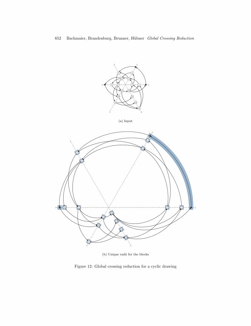
Level graphs can be generalized to cyclic and to radial level graphs. In cycliclevel graphs the set of levels is ordered in a cyclic way, i. e., the first level directlysucceeds the last. This corresponds to the recurrent hierarchies of Sugiyama etal. [43]. Cyclic levels are normally drawn forming a star in 2D (see Fig. 12(a)).These drawings explicitly visualize cycles in graphs [6], which is helpful, e. g.,in scheduling [26, 41, 44] and in bioinformatics [35]. In radial level graphs eachlevel itself is ordered in a cyclic way, i. e., the first vertex in each level is theright neighbor of the last vertex. The levels are drawn as concentric rings. SeeFigs. 12 and 13 for example drawings. Global sifting can be extended to bothconcepts and is the first crossing reduction technique avoiding type 2 conflictsin each case.

For cyclic level graphs our global sifting can be used without any changesand within the same time complexity. Note that one-sided 2-level algorithmscannot be applied here, since each of them pushes most of the crossings to thenext level and these form a cycle. Even the absence of type 2 conflicts cannotbe guaranteed then, because the sweep has to stop at some level. There is nopossibility to push the crossings and the type 2 conflicts upwards or downwardsout of the drawings as it is in usual hierarchical level drawings. The conflictsmove like a wave front from level to level and they recur.

For leveling and coordinate assignment of cyclic level graphs see [2, 4]. TheILP approach by Junger et al. [29] can be used for exact cyclic k-level crossingminimization straightforward by including additional constraints for the edgesbetween the last and the first level.

In a radial level graph the levels are concentric circles (see Fig. 13(a)). Thesedrawings visualize distance or importance, and are the common drawings ofsocial networks [9,46]. They map structural centrality of the graph to geometriccentrality. Crossing minimization in radial level graphs is NP-hard, even ifrestricted to two levels with one side fixed [1]. Our global sifting approachguarantees radially aligned long edges and can be used with minor modifications:Each block of the block list B has its own angle. The order of B starts withan arbitrary block. As in [1] we define an offset ψ : E → Z for each outersegment. The absolute value |ψ(e)| counts the crossings of segment e withan imaginary ray splitting the levels by a straight halfline from the concentriccenter to infinity. If ψ(e) < 0 (ψ(e) > 0), e has clockwise (counter-clockwise)direction from the source to the target. When sifting a block A ∈ B, we haveto update the partings, which are the two borders between the counterclockwiseand clockwise segments in the levels above and below A, see Fig. 13(b). Sincewe can do this independently of each other and add the results of the changein crossings to ∆ in Algorithm 4, we use the same technique as in [1]. We sifta block from its current position in counterclockwise direction. Thus, for fewcrossings the partings have to follow this direction in their levels. During theswap the test whether or not changing the orientation of some of the first of the(ordered) incident segments of A by incrementing their offsets, and thus puttingthem last, leads to less crossings. However, counting the difference raises the


1

23

4

5 6

2

4

6

8

10

1

3

5

7

11

12

13

14

15

9

(a) Input

1

2

3

4

5 6

2

4

6

8

10

1

3

5

7

11

12

13

14

15

9

(b) Unique radii for the blocks

Figure 12: Global crossing reduction for a cyclic drawing

JGAA, 15(5) 631–659 (2011) 653

1

2

3

4

5 6

2

4

6

8

10

1

3

5

7

11

12

13

14

15

9

(c) After global sifting

1

23

4

5 6

2

46

8

10

1

35

7

11

12

13

14

15

9

(d) Resulting Embedding

Figure 12: Global crossing reduction for a cyclic drawing (cont.)


overall running time to O(|E|3). The radial coordinate assignment phase in [1]relies on the obtained absence of type 2 conflicts.

6 Discussion

We have presented an algorithm for the global crossing reduction problem of k-level graphs. It produces high quality results with fewer crossings than commonapproaches at the expense of a quadratic running time which is still feasible inpractice. Global crossing reduction was an open problem since the introductionof the hierarchical framework [43] in 1981. For radial and cyclic level crossingreduction our algorithm is the first which guarantees the absence of type 2 con-flicts. Our approach simplifies and improves several other algorithms concerninglevel planarity and crossing reduction.

6.1 Open Problems

The practical time complexity of the global sifting algorithm could be improvedby testing the positions of blocks which change a relative order on a level only.Often blocks on disjoint levels are swapped which does not change any permu-tation on any level. The worst case situation is having a level with only onevertex v. The global sifting algorithm tests all O(|E|) positions for the block ofv although each of them yields the same permutation of the level of v. Each suchswap is computed in constant time. Nevertheless, avoiding unnecessary swapsis desirable, although it will not improve the theoretical worst case complexity:Consider a complete bipartite graph G = (V1 ∪V2, E) with the vertices of V1 onlevel 1 and the vertices of V2 on level 3. Then, level 2 contains O(|E|) = O(|V |2)dummy vertices. For each block representing a dummy vertex, O(|E|) positionson level 2 have to be tested. Hence, having a time complexity of O(|E|2) whenavoiding unnecessary swaps is possible as well, even if O(|E|) = O(|V |2).

A conceptually rather simple approach to reduce the number of unnecessaryswaps is to stop a sifting step if all adjacent blocks of the current block A are leftof A already. Swapping A further to the right can only increase the number ofcrossings then. Similarly, the first position to test for a block A can be directlyleft of its leftmost adjacent block.

A first approach to applying the blocks to the radial crossing reductionalgorithm in [1] leads to a time complexity of O(|E|3). Further research isneeded to evaluate if a time complexity of O(|E|2) can be achieved in the radialcase as well.

JGAA, 15(5) 631–659 (2011) 655

34

12

1

3

2

5

7

10

4

8

11

6

9

(a) Input

34

12

1

3

5

11

7

4

8

6

9

2

10 1-

1

0

1 1-

1-

1-

0

(b) Unique block angles

34

12

1

3

5

11

7

4

6

9

2

10 8

(c) After global sifting

v

34

12

3

5

7

6

2

10

11

9

8

4

1

(d) Resulting Embedding

Figure 13: Global crossing reduction for a radial drawing


References

[1] C. Bachmaier. A radial adaption of the sugiyama framework for visualizinghierarchical information. IEEE Trans. Vis. Comput. Graphics, 13(3):583–594, 2007.

[2] C. Bachmaier, F. J. Brandenburg, W. Brunner, and R. Fulop. Coordinateassignment for cyclic level graphs. In H. Q. Ngo, editor, Proc. Computingand Combinatorics, COCOON 2009, volume 5609 of LNCS, pages 66–75.Springer, 2009.

[3] C. Bachmaier, F. J. Brandenburg, W. Brunner, and F. Hubner. A global k-level crossing reduction algorithm. In M. S. Rahman and S. Fujita, editors,Proc. Workshop on Algorithms and Computation, WALCOM 2010, volume5942 of LNCS, pages 70–81. Springer, 2010.

[4] C. Bachmaier, F. J. Brandenburg, W. Brunner, and G. Lovasz. Cyclicleveling of directed graphs. In I. G. Tollis and M. Patrignani, editors, Proc.Graph Drawing, GD 2008, volume 5417 of LNCS, pages 348–349. Springer,2009.

[5] C. Bachmaier, F. J. Brandenburg, M. Forster, P. Holleis, and M. Raitner.Gravisto: Graph visualization toolkit. In J. Pach, editor, Proc. GraphDrawing, GD 2004, volume 3383 of LNCS, pages 502–503. Springer, 2004.

[6] C. Bachmaier and W. Brunner. Linear time planarity testing and em-bedding of strongly connected cyclic level graphs. In D. Halperin andK. Mehlhorn, editors, ESA 2008, volume 5193 of LNCS, pages 136–147.Springer, 2008.

[7] C. Bachmaier, W. Brunner, and A. Gleißner. Grid sifting: Leveling andcrossing reduction. Submitted for publication.

[8] M. Baur and U. Brandes. Crossing reduction in circular layout. InJ. Hromkovic, M. Nagl, and B. Westfechtel, editors, Proc. Workshop onGraph-Theoretic Concepts in Computer Science, WG 2004, volume 3353 ofLNCS, pages 332–343. Springer, 2004.

[9] U. Brandes and T. Erlebach, editors. Network Analysis: MethodologicalFoundations, volume 3418 of LNCS Tutorial. Springer, 2005.

[10] U. Brandes and B. Kopf. Fast and simple horizontal coordinate assignment.In P. Mutzel, M. Junger, and S. Leipert, editors, Proc. Graph Drawing, GD2001, volume 2265 of LNCS, pages 31–44. Springer, 2002.

[11] M. Chimani, C. Gutwenger, P. Mutzel, and H.-M. Wong. Layer-free upwardcrossing minimization. ACM J. Exp. Alg., 15:2.2.1–2.2.27, 2010.

[12] M. Chimani, C. Gutwenger, P. Mutzel, and H.-M. Wong. Upward pla-narization layout. In D. Eppstein and E. R. Gansner, editors, Proc. GraphDrawing, GD 2009, volume 5849 of LNCS, pages 94–106. Springer, 2010.

JGAA, 15(5) 631–659 (2011) 657

[13] E. G. Coffman Jr. and R. L. Graham. Optimal scheduling for two processorsystems. Acta Informatica, 1(3):200–213, 1972.

[14] G. Di Battista, P. Eades, R. Tamassia, and I. G. Tollis. Graph Drawing:Algorithms for the Visualization of Graphs. Prentice Hall, 1999.

[15] G. Di Battista, A. Garg, G. Liotta, A. Parise, R. Tamassia, E. Tassinari,F. Vargiu, and L. Vismara. Drawing directed acyclic graphs: An experi-mental study. Internat. J. Comput. Geom. Appl., 10(6):623–648, 2000.

[16] G. Di Battista, A. Garg, R. Tamassia, E. Tassinari, and F. Vargiu. Anexperimental comparison of four graph drawing algorithms. Comput. Geom.Theory Appl., 7(5–6):303–325, 1997.

[17] P. Eades and D. Kelly. Heuristics for reducing crossings in 2-layered net-works. Ars Combinatorica, 21(A):89–98, 1986.

[18] P. Eades and K. Sugiyama. How to draw a directed graph. J. Inform.Process., 13(4):424–437, 1990.

[19] P. Eades and N. C. Wormald. Edge crossings in drawings of bipartitegraphs. Algorithmica, 11(1):379–403, 1994.

[20] M. Eiglsperger, F. Eppinger, and M. Kaufmann. An approach for mixedupward planarization. J. Graph Alg. App., 7(2):203–220, 2003.

[21] M. Eiglsperger, M. Siebenhaller, and M. Kaufmann. An efficient imple-mentation of sugiyama’s algorithm for layered graph drawing. J. GraphAlg. App., 9(3):305–325, 2005.

[22] T. Eschbach, W. Gunther, R. Drexler, and B. Becker. Crossing reductionby windows optimization. In M. T. Goodrich and S. G. Kobourov, editors,Proc. Graph Drawing, GD 2002, volume 2528 of LNCS, pages 285–294.Springer, 2002.

[23] M. Forster. Crossings in Clustered Level Graphs. PhD thesis, University ofPassau, 2004.

[24] M. Forster and C. Bachmaier. Clustered level planarity. In P. VanEmde Boas, J. Pokorny, M. Bielikova, and J. Stuller, editors, Proc. Soft-ware Seminar: Theory and Practice of Informatics, SOFSEM 2004, volume2932 of LNCS, pages 218–228. Springer, 2004.

[25] M. R. Garey and D. S. Johnson. Crossing number is NP-complete. SIAMJ. Alg. Discr. Meth., 4(3):312–316, 1983.

[26] N. G. Hall, T.-E. Lee, and M. E. Posner. The complexity of cyclic shopscheduling problems. Journal of Scheduling, 5(4):307–327, 2002.


[27] M. Harrigan and P. Healy. Practical level planarity testing and layoutwith embedding constraints. In S.-H. Hong, T. Nishizeki, and W. Quan,editors, Proc. Graph Drawing, GD 2007, volume 4875 of LNCS, pages 62–68. Springer, 2008.

[28] F. Hubner. A global approach on crossing minimization in hierarchical andcyclic layouts of leveled graphs. Master’s thesis, University of Passau, 2009.

[29] M. Junger, E. K. Lee, P. Mutzel, and T. Odenthal. A polyhedral approachto the multi-layer crossing minimization problem. In G. Di Battista, edi-tor, Proc. Graph Drawing, GD 1997, volume 1353 of LNCS, pages 13–24.Springer, 1997.

[30] M. Junger and P. Mutzel. 2-layer straightline crossing minimization: Per-formance of exact and heuristic algorithms. J. Graph Alg. App., 1(1):1–25,1997.

[31] M. Kaufmann and D. Wagner. Drawing Graphs, volume 2025 of LNCS.Springer, 2001.

[32] P. Kuntz, B. Pinaud, and R. Lehn. Minimizing crossings in hierarchicaldigraphs with a hybridized genetic algorithm. J. Heuristics, 12(1–2):23–26, 2006.

[33] M. Laguna, R. Martı, and V. Valls. Arc crossing minimization in hier-archical digraphs with tabu search. Comp. Oper. Res., 24(12):1175–1186,1997.

[34] C. Matuszewski, R. Schonfeld, and P. Molitor. Using sifting for k-layerstraightline crossing minimization. In J. Kratochvıl, editor, Proc. GraphDrawing, GD 1999, volume 1731 of LNCS, pages 217–224. Springer, 1999.

[35] G. Michal, editor. Biochemical Pathways: An Atlas of Biochemistry andMolecular Biology. Wiley, 1998.

[36] X. Munoz, W. Unger, and I. Vrt’o. One sided crossing minimization is NP-hard for sparse graphs. In P. Mutzel, M. Junger, and S. Leipert, editors,Proc. Graph Drawing, GD 2001, volume 2265 of LNCS, pages 115–122.Springer, 2002.

[37] H. Nagamochi. An improved bound on the one-sided minimum crossingnumber in two-layered drawing. Discrete Comput. Geom., 33:569–591,2005.

[38] S. North. AT&T Graph Collection. http://www.graphdrawing.org/.

[39] B. Randerath, E. Speckenmeyer, E. Boros, P. Hammer, A. Kogan,K. Makino, B. Simeone, and O. Cepek. A satisfiability formulation ofproblems on level graphs. Elect. Notes in Discr. Math., 9:269–277, 2001.

http://www.graphdrawing.org/

JGAA, 15(5) 631–659 (2011) 659

[40] R. Rudell. Dynamic variable ordering for ordered binary decision diagrams.In Proc. IEEE/ACM International Conference on Computer Aided Design,ICCAD 1993, pages 42–47. IEEE Computer Society Press, 1993.

[41] P. Serafini and W. Ukovich. A mathematical model for periodic schedulingproblems. SIAM J. Discr. Math., 2(4):550–581, 1989.

[42] M. Stallmann, F. Brglez, and D. Ghosh. Heuristics, experimental subjects,and treatment evaluation in bigraph crossing minimization. ACM J. Exp.Alg., 6(8), 2001.

[43] K. Sugiyama, S. Tagawa, and M. Toda. Methods for visual understand-ing of hierarchical system structures. IEEE Trans. Syst., Man, Cybern.,11(2):109–125, 1981.

[44] E. R. Tufte. The Visual Display of Quantitative Information. GraphicsPress, 2nd edition, 2001.

[45] J. Utech, J. Branke, H. Schmeck, and P. Eades. An evolutionary algorithmfor drawing directed graphs. In H. R. Arabnia, editor, Proc. InternationalConference on Imaging Science, Systems, and Technology, CISST 1998,pages 154–160. CSREA, 1998.

[46] S. Wasserman and K. Faust. Social Network Analysis: Methods and Appli-cations (Structural Analysis in the Social Sciences). Cambridge UniversityPress, 1994.

global k-level crossing reduction - emis · 632 bachmaier, brandenburg, brunner, hub ner global...

Documents