global image measurements - uzh · the science of stereology relates the measurements that can be...

T he distinction between image processing, which has occupied most of the preceding chap-ters, and image analysis lies in the extraction of information from the image. As mentionedseveral times previously, image processing, like word processing (or food processing) is the

science of rearrangement. Pixel values may be altered according to neighboring pixel brightnesses,or shifted to another place in the array by image warping, but the sheer quantity of pixels is un-changed. So in word processing it is possible to cut and paste paragraphs, perform spell-checking,or alter type styles without reducing the volume of text. And food processing is also an effort at re-arrangement of ingredients to produce a more palatable mixture, not to boil it down to the essenceof the ingredients. Image analysis, by contrast, attempts to find those descriptive parameters, usu-ally numeric, that succinctly represent the information of importance in the image.

The processing steps considered in earlier chapters are in many cases quite essential to carrying outthis task. Defining the features to be measured frequently requires image processing to correct ac-quisition defects, enhance the visibility of particular structures, threshold them from the back-ground, and perform further steps to separate touching objects or select those to be measured. Andwe have seen in several of the earlier chapters opportunities to use these processing methodsthemselves to obtain numeric information.

Global measurements and stereologyThere are two major classes of image measurements: ones performed on the entire image field(sometimes called the “scene”), and ones performed on each of the separate features present. Thelatter feature-specific measurements are covered in the next chapter. The first group of measure-ments are most typically involved in the characterization of three-dimensional structures viewed assection planes in the microscope, although the methods are completely general and some of therelationships have been discovered and are routinely applied by workers in earth sciences and as-tronomy. The science of stereology relates the measurements that can be performed on two-di-mensional images to the three-dimensional structures that are represented and sampled by thoseimages. It is primarily a geometrical science, whose most widely used rules and calculations havea deceptive simplicity. Reviews of modern stereological methods can be found in (Russ and De-hoff, 2001; Howard and Reed, 1998; Kurzydlowski and Ralph, 1995), while classical methods aredescribed in (Dehoff and Rhines, 1968; Underwood, 1970; Weibel, 1979; Russ, 1986).

Global Image Measurements8

1142_CH08 pp445 4/26/02 8:58 AM Page 445

© 2002 by CRC Press LLC

446 The Image Processing Handbook

The simplest and perhaps most frequently used stereological procedure is the measurement of thevolume fraction that some structure occupies in a solid. This could be the volume of nuclei incells, a particular phase in a metal, porosity in ceramic, mineral in an ore, etc. Stereologists oftenuse the word “phase” to refer to the structure in which they are interested, even if it is not a phasein the chemical or thermodynamic sense. If a structure or phase can be identified in an image, andthat image is representative of the whole, then the area fraction which the phase occupies in theimage is a measure of the volume fraction that it occupies in the solid. This relationship is, in fact,one of the oldest known relationships in stereology, used in mineral analysis 150 years ago.

Of course, this requires some explanation and clarification of the assumptions. The image must berepresentative in the sense that every part of the solid has an equal chance of being examined, sothe sections must be uniformly and randomly placed in the solid. Trying to measure the volumefraction of bone in the human body requires that head, torso, arms, and legs all have an equalchance of being viewed; that is the “uniform” part of the assumption. Random means, simply, thatnothing is done to bias the measurements by including or excluding particular areas in the images.For example, choosing to measure only those images in which at least some bone was visiblewould obviously bias the measurements. More subtle, in many cases, is the tendency of micro-scopists to select areas for imaging that have some aesthetic quality (collecting pretty pictures). Al-most certainly this will tend to bias the results. A proper random stereological sampling proceduredoes not allow the human to select or shift the view.

Many published papers in all fields of science that use microscopy include images with the cap-tion “representative microstructure” or “typical microstructure,” and in no case is this likely to betrue. Either the particular image selected has been chosen because it shows most clearly somefeature of the structure that the author believes is important, or it displays the best qualities ofspecimen preparation and image contrast, or some other characteristic that makes it (almost by de-finition) non-typical. In most real structures, there is no such thing as one typical field of view ina true statistical sense. That is why it is important to collect many images from multiple fields ofview, spread throughout the specimen in an unbiased way. Data are collected from many fieldsand combined to represent the entire structure.

Assuming that one image could be a uniform, random sample of the structure, then the “expectedvalue” of the area fraction of the structure is equal to the volume fraction. Of course, in any givenimage that may not be the result. In some images, the phase or structure of interest may not evenbe present, while in others it may occupy the entire field of view. In general it is necessary to se-lect an appropriate magnification so that the structures are visible, and to examine multiple fieldsof view and to average the measurements. The average then approaches the true value as moremeasurements are included.

One way to measure the area fraction of a structure is, of course, to use the image histogram. If thephase has a unique grey scale or color value, then the area of peak in the histogram provides a di-rect measure of the number of pixels covered, and hence the total area, regardless of whether itoccupies one large or many small regions in the image. As shown in previous chapters, however,it is common to require image processing before thresholding can selectively delineate a structure,and to require editing of the binary image after thresholding. These steps also affect the area mea-surement, so in most cases the determination of area fraction must be made from the final binaryimage. All that is required is to count the black and white pixels.

Although this is a simple procedure, it is difficult to assess the accuracy of the measurement. Pix-els along the boundaries of features or regions present a challenge because thresholding and sub-sequent morphological processing may include or exclude them from the total. An image consist-ing of a single large, compact region has many fewer edge pixels (and thus less potential

1142_CH08 pp445 4/26/02 8:58 AM Page 446


measurement error) than an image in which the same total area is distributed as many small or ir-regular features (Figure 1).

There is a preferred way to determine area fraction (and hence volume fraction) that is very effi-cient and does allow an estimation of the measurement precision. Traditionally, this method hasbeen performed manually, but it is also easy to accomplish using a computer. A grid of points issuperimposed on the image, and the fraction of the points that fall on the structure of interest iscounted. The expected value of this point fraction is also the volume fraction. Often, the numberof points in the grid is very small so that manual counting can be done at a glance. The grid maybe on an eyepiece reticule in the microscope, or overlaid on a video screen or photograph, or gen-erated within the computer. The points should be far enough apart that they provide independentmeasures of the structure (in other words, at the image magnification being used, two pointsshould rarely fall into the same feature). If the structure is random, then any grid of points can beused and a regular square grid is convenient. If the structure is highly regular, then the grid itselfshould be randomized to prevent bias as discussed above.

When a grid is superimposed on the original grey-scale or color image (with whatever enhance-ment has been provided by processing), the human viewer can use independent knowledge andjudgment to decide whether each point is within the region of interest. People are very good atthis. But they are not very good at counting, so it may still be useful to have the human mark thepoints and the computer perform the counting operation as shown in Figure 2.

Chapter 8: Global Image Measurements 447

Figure 1. Two images with thesame area fraction (26%)of black pixels: (a) one large compactregion; (b) many small irregularfeatures. The measurementprecision depends on the totalperiphery of the black-whiteboundary. It is alsointeresting to note that mosthuman observers do notestimate area fractions veryaccurately, nor judge thatthese two images have thesame area of black pixels.

a b

Figure 2. Computer counting of marks. A humanhas placed color marks near the grid points(intersection of the lines) that fall on each phaseof interest, and the computer has counted them.For the white phase, the estimated volumefraction is 15/35 = 42.8%.

1142_CH08 pp445 4/26/02 8:58 AM Page 447



The points become a probe into the three-dimensional microstructure, and the number of pointsthat “hit” the phase of interest allows an estimate of the measurement precision, since for inde-pendent events the standard deviation is just the square root of the count. This permits making aquick estimate of the number of images (multiple fields of view on multiple sections) that will beneeded to achieve the desired final measurement precision. For example, if a grid of 25 points isused (a 5 × 5 array), and about 5 points, on average, lie on the phase of interest, that correspondsto a volume fraction of 20%. To determine the actual value with a relative precision of (say) 5% (inother words 20±1% volume fraction) it is only necessary to apply the grid to multiple fields ofview until a total of 400 hits have been tallied (the square root of 400 is 20, or 5%). This would re-quire about 80 fields of view (400/5).

A grid of points can also be efficiently applied to a thresholded and processed binary image usingBoolean logic as shown in Chapter 7. If the grid is combined with the binary image using aBoolean “AND,” and the surviving points are counted, the result is just those points that fell ontothe phase of interest as shown in Figure 3. The accepted notation for these relationships is

(1)

meaning that the volume of the phase of interest per unit volume of material, VV, equals (or moreprecisely is measured by) the area fraction AA or the point fraction PP.

Volume fraction is a dimensionless ratio, so the magnification of the image need not be known ex-actly. However, it is also possible to measure the volume of a specific structure by cutting a seriesof sections through it and measuring the area in each section (Gundersen, 1986). As shown inFigure 4, the volume of the sampled space is defined by the size and spacing of the sections, andthe number of “hits” made by the grid points provides an absolute measure of the feature volume.Each grid point samples the structure and represents a volume in space equal to the area of a gridsquare times the section spacing. In this case, of course, the magnification must be calibrated.

In many cases, as shown in Figure 5, it is necessary to measure two volumes, that of the structureof interest and of an enclosing structure. In the example, a sectioned rat lung, the area of lung

V A PV A P= =

Figure 3. Binary image of the white phase in the metal structure from Figure 2, with a superimposed pointgrid (points enlarged for visibility). A Boolean AND of the two images leaves just the points that lie on thephase (b), which the computer then counts to determine PP = 64/154 = 41.5%. The density of pointsillustrated in this image is somewhat too high for optimum precision estimation, because cases occur inwhich multiple points fall on the same feature.

a b

1142_CH08 pp445 4/26/02 8:58 AM 48



VolumeFilled Area Net Area

Filled Area=

−∑∑∑

S BV A= π4

Figure 4. Cavalieri’s method for measuring the volume of an object.The grids on each section plane divide the object into cells.Counting the grid points that fall on the structure of interestprovides a measure of the number of cells within the structure, andhence a measure of the volume. In the example, if the planespacing (h) is 5 µm and the grid spacing (d) is 2 µm, then eachcell has a volume of 5 × 2 × 2 = 20 µm3, and the total number ofhits (17 + 20 + 19 + 21 + 17 = 94) estimates the total volume as1880 µm3. Measuring the area of each intersection andintegrating the volume with Simpson’s rule gives an estimate of1814 µm3.

Figure 5. Onesection of ratlung tissue: (a) originalimage; (b) leveled; (c) thresholded;(d) internal gapsfilled. The areas ofimages c and d areused to determinethe void volumewithin the lung.

a b

c d

1142_CH08 pp445 4/26/02 8:58 AM Page 449



tissue in each section is added including internal voids, and the net area is also summed. The voidarea within the lung is then calculated as

(2)

Surface areaAnother global parameter that is easily measured stereologically is the surface area. Surfaces canbe the boundary between two structures, such as the surface area of the nucleus, the total area ofcell wall in plant tissue, the total grain boundary area in a metal, or the surface of porosity in a ce-ramic. Note that in some of these examples the surface separates two different phases or structures,while in others it separates different regions (cells or grains) that are the same in structure and com-position. Surfaces are usually very important in structures, because they are the interfaces wherechemistry and diffusion take place, and control many properties such as strength, fracture, lightscattering, etc.

In a two-dimensional section image through a three-dimensional structure, boundaries and surfacesare seen as lines. The total length of these lines is proportional to the amount of surface area pre-sent in the three-dimensional solid. The surface may not intersect the section plane perpendicularly,in fact in general it will not. If the surfaces are isotropic (have an equal probability of being ori-ented in any direction), then the relationship between total surface area per unit volume of sam-ple and the total length of line per unit area of image is

(3)

where SV is the accepted notation for the surface area per unit volume, and BA denotes the totallength of boundary per unit area of image. Notice that both terms have dimensions of 1/length, andthat it is consequently important to know the image magnification. Figure 6 shows an example.The boundary lines (colored) have a total length of 9886 µm, and the image area is 15,270 µm2.This gives a calculated surface area per unit volume of 0.0824 µm2/µm3, or 82.4 mm2/mm3.

Once again, it is difficult to specify the precision of such a measurement. Measuring the length ofa boundary line in a digitized image is one of the most error-prone tasks in image measurementbecause of the pixellation of the image and the common observation that as magnification is in-creased, more irregularities in the boundary become visible and the measured boundary length in-creases. The preferred method for determining surface area is consequently to place a grid of lineson the image and to count the number of intersection points which they make with the line rep-resenting the surface of interest. The relationship between the surface area per unit volume (SV,square micrometers per cubic micrometer) and the number of intersections (PL, number per mi-crometer) is just

(4)

where the factor 2 compensates for the various angles at which the grid lines can intersect theboundary. Again, because this is now a counting experiment, the measurement precision can beestimated from the square root of the number of intersection points, provided that the lines (whichare the probes into the microstructure in this measurement) are far enough apart that the inter-sections are independent events.

VolumeFilled Area Net Area

Filled Area=

−∑∑∑

S BV A= π4

S PV L= ⋅2

1142_CH08 pp445 4/26/02 8:58 AM Page 450


Generating a grid of lines on the same image as in Figure 6 and counting intersections (Figure7) produces a similar measurement result as the boundary line technique. The total length of thegrid lines is 4646 µm. Performing a Boolean AND and counting the intersections gives 197 hits(some are a single pixel and some more than one, depending on the angle between the bound-ary and the line). Using Equation 4, this corresponds to a surface area per unit volume of 0.0848µm2/µm3. Based on the number of counts, the estimated relative precision is ±7.2% (0.0848 ±0.0061 µm2/µm3).

Placing grid lines on images and counting intersections can be performed in all of the sameways (manually, manual marking with computer counting, or automatically using Boolean logic)as discussed above for point counting. The problem with this method as described is that it re-lies on the assumption that the surfaces being measured are isotropic. In real structures this cri-terion is rarely met. Consequently, if the structure is not isotropic, then it is necessary to constructa grid of lines that does sample the structure isotropically (in addition to the requirements of uni-form and random sampling noted above). Many of the developments in modern stereology areaimed at finding practical ways to meet this isotropic, uniform, random (IUR) requirement. To vi-sualize the meaning of isotropic directions, consider a hemisphere as shown in Figure 8. Eachdirection in space is represented by a point on the sphere. Points should be distributed evenlyacross the spherical surface.


Figure 6. The boundary lines around the white phase in thesame image as Figures 2 and 3 can be isolated using thetechniques from Chapter 7, and measured to determine thesurface area as described in the text.

Figure 7. ANDing a grid of lines with the boundary lines from Figure 6 and counting the intersections alsomeasures the surface area, as described in the text.

a b

1142_CH08 pp445 4/26/02 8:58 AM Page 451



The most successful approach to generating isotropic, uniform and random lines to probe the sur-faces in a three dimensional structure is called “vertical sectioning” (Baddeley et al., 1986). It re-quires selecting some direction in the structure that can always be identified. This might be the axisof the backbone in an animal, or the normal to a surface in a rolled metal sheet, or the directionof gravity for sedimentary layers of rock. Then all sections are cut parallel to this direction, but ro-tated uniformly and randomly about it, as shown in Figure 9. Note that this is emphatically not theway most sections are cut when biological tissue is embedded and microtomed (those sections areall perpendicular to the same direction). It would also be possible to cut the vertical sections as apie is normally cut, with radial slices, but these would oversample the center of the pie comparedto the periphery.

The vertical axis direction is present on all sections, so these cut planes are directionally biased. Iflines were drawn on these sections with uniform directions in the plane, as shown in Figure 10,they would cluster near the north pole on the hemisphere. Directions near the equator would beundersampled. That bias can be compensated by drawing lines that are sine-weighted, as shownin Figure 11. Instead of drawing lines in uniform angle steps, they are drawn with uniform stepsin the sine of the angle. This produces more directions around the equator and spreads out the di-rections near the north pole so that the points are uniformly distributed on the sphere. While a setof radial lines as shown in the figure is isotropic, it is not uniform (the center is oversampled andthe corners undersampled).

Figure 8. A hemisphere showing a direction in three-dimensional space represented by a point on the sphere.

Figure 9. Method for cutting vertical sections: (a) correct — all sections are parallel to and rotated uniformly about a single selected axis; (b) incorrect — sections are all perpendicular to a common direction.

ab

1142_CH08 pp445 4/26/02 8:58 AM Page 452


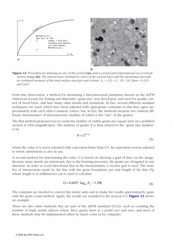
The most convenient way to draw sine-weighted lines that uniformly sample the area is to gener-ate cycloids as shown in Figure 12. The cycloid is the path followed by a point on the circum-ference of a rolling circle. It is sine-weighted and when drawn on vertical sections has exactly thecorrect set of orientations to provide isotropic sampling of directions in the three-dimensional solidfrom which the sections were cut. Counting the intersections made by the cycloid grid with theboundary lines in the image provides the PL value needed to calculate the surface area per unit vol-ume. The length of each quarter arc of the cycloid line is just twice its height.

If the specimen is actually isotropic, the method of cutting vertical sections and counting intersec-tions using a grid of cycloids will produce the correct answer, at the expense of doing a bit morework (mostly in sample preparation) than would have been needed if the isotropy was known be-forehand. But if the specimen has any anisotropy, the easy method of cutting parallel sections anddrawing straight line grids would produce an incorrect answer with an unknown amount of bias,while the vertical section method gives the true answer.

ASTM Grain SizeMore than 100 years ago, when naval gunnery was introducing larger and larger guns onto bat-tleships, brass cartridge casings were used to hold the gunpowder and projectile, essentially an en-larged version of a modern rifle cartridge. It was observed that after firing it was sometimes diffi-cult to extract the used brass cartridge from the gun chamber, because the material fractured whenit was pulled from the rear rim. The metal flowed and thinned when the charge was detonated, andclearly some difference in material structure was related to the tendency to tearing.


Figure 10. Drawing lines withuniform angles on eachplane, and the resultantclustering of directionsnear the north pole of thehemisphere of orientations.

Figure 11. Drawing lines withsine-weighted angles oneach plane, and theresultant uniformdistribution of orientationsin three-dimensional space.

1142_CH08 pp445 4/26/02 8:58 AM Page 453



From that observation, a method for measuring a microstructural parameter known as the ASTM(American Society for Testing and Materials) “grain size” was developed, and used for quality con-trol of naval brass, and later many other metals and nonmetals. In fact, several different standardtechniques are used, which have been adjusted with appropriate constants so that they agree ap-proximately with each other’s numeric values; but, in fact, the methods measure two entirely dif-ferent characteristics of microstructure (neither of which is the “size” of the grains).

The first method proposed was to count the number of visible grains per square inch on a polishedsection at 100x magnification. The number of grains N is then related to the “grain size number”G by

(5)

where the value G is never reported with a precision better than 0.5. An equivalent version adjustedto metric dimensions is also in use.

A second method for determining the value G is based on drawing a grid of lines on the image.Because many metals are anisotropic due to the forming processes, the grains are elongated in onedirection. In order to avoid directional bias in the measurement, a circular grid is used. The num-ber of intersections made by the line with the grain boundaries per unit length of the line (NLwhere length is in millimeters) can is used to calculate

(6)

The constants are needed to convert the metric units and to make the results approximately agreewith the grain count method. Again, the results are rounded to the nearest 0.5; Figure 13 showsan example.

There are also other methods that are part of the ASTM standard (E112), such as counting thenumber of triple points (places where three grains meet at a point) per unit area, and most ofthese methods may be implemented either by hand count or by computer.

x = π

y = 2

Length = 4

MoveTo(0,0);For k=1 to 100{ theta = k*π/100;

x=theta-sin(theta);y=1-cos(theta);MoveTo(x,y);

}

Figure 12. Procedure for drawing an arc of the cycloid (a), and a cycloid grid superimposed on a verticalsection image (b). The intersections (marked in color) of the cycloid lines with the membranes providean unbiased measure of the total surface area per unit volume, SV = 2 PL = 2 · 39 / 331.5µm = 0.235µm2/µm3.

a

b

N G= −2 1( )

G NL= ⋅ −6 6457 3 29810. log .

1142_CH08 pp445 4/26/02 8:58 AM Page 454


The intercept count method (Equation 6) in reality measures the total surface area of grain bound-ary. Note the use of NL which, similar to the PL value in Equation 4, is proportional to the surfacearea per unit volume. The importance of grain boundary area makes sense from a mechanicalproperty standpoint since creep in materials occurs due to grain boundary sliding and grain rota-tion, and grain deformation occurs by motion of dislocations which start and end at these sameboundaries. The grain count and triple-point count methods actually measure the total length perunit volume of the edges of grains, which is a parameter related primarily to diffusion. Measure-ment of the length of structures is discussed in the following paragraphs.

The fact that one of these parameters can be even approximately tied to the other is due to the lim-ited application of the method to metals that have been heat-treated so that they are fully recrys-tallized. In this condition, the distribution of actual three-dimensional grain sizes approaches aconstant, more-or-less log-normal state in which the structure may coarsen with time (large grainsgrow and small ones vanish) but the structure remains self similar. Hence there is an approxi-mately consistent relationship between the length of edges and the area of surfaces.

The same relationship does not apply to metals without this heat treatment, and so the notion ofa single numerical value that can characterize the microstructure is flawed, even for quality con-trol purposes, and the measurement method used does matter. But 100 years of use have sancti-fied the technique and most practitioners are not aware of what their procedure actually measuresin the microstructure.

Actually measuring the “size” (usually the volume) of individual grains or cells in a three-dimen-sional solid is quite difficult. It has been done in a few cases by literally taking the material apart(e.g., by chemically dissolving a thin layer along the boundaries so the grains are separated), andmeasuring each one. Other researchers have used an exhaustive serial sectioning technique thatproduces a complete three-dimensional volumetric image of the structure, from which measure-ments can be made. Both of these approaches are far too laborious for routine practical use. De-termining the mean volume of cells can be done using the Disector method described below. Thisactually measures the number per unit volume, but the inverse of that quantity is the mean volumeper feature. This method relies heavily on computer-based image processing to deal with the largenumber of images. Figure 14, below, will show an example.


Figure 13. Light microscope image of a low carbon steel (a), which is prepared by leveling, thresholdingand skeletonizing to delineate the grain boundaries (b). Counting the number of grains inside thelargest circle (445, counting each one that intersects the circle as 1/2) gives a grain size number G = 8.7.Counting the intercepts with the concentric circle grids (147 with a grid length of 2300 µm) gives agrain size number G = 9.1. Both values would normally be reported as a grain size number of 9.

a b

1142_CH08 pp445 4/26/02 8:58 AM Page 455



It is also possible to measure the variance of the size distribution of the features using a point-sampledintercept method applied to IUR section planes, described below. But if the actual size distribution ofthe three-dimensional features is needed, then the more intensive methods must be undertaken.

Multiple types of surfacesIn most kinds of real samples, there are several different phases or structures present, and conse-quently many different types of boundary surfaces. In a three-phase material, containing regionswhich for convenience can be identified as types α, β and γ, there are six possible interfaces ( α-α, α-β, α-γ, β-β, β-γ, and γ-γ) and the number goes up rapidly in more complex structures. Someof the possible interface types may be absent, meaning that those two phase regions never touch(e.g., nuclei in separate cells do not touch each other, it makes no sense to consider a surface be-tween two pores, etc.). Measuring the amounts of each different type of interface can be very use-ful in characterizing the overall three-dimensional structure.

Figure 14 shows a three-phase metal structure. Notice that no white dendritic region touches an-other one, for example. Chapter 7 showed how Boolean logic with the dilated region outlines canbe used to delineate each type of interface. Once the image of the boundaries has been isolated,counting intersections with a grid provides the measurement of surface area per unit volume.

Figure 15 shows a simpler, idealized, two-phase microstructure. By thresholding each phase, us-ing morphological operations such as a closing, and Boolean logic to combine two derived images,each of the three distinct boundary types can be isolated (in the image, they have been combined

Figure 14. The three-phase aluminum-zinc alloy fromFigure 2, with the phase boundaries shown in color.

Figure 15. Idealized drawing of a two-phase microstructure (a) the three different types of interface boundaries present (b) and the result of counting the intersections of these boundaries with a cycloid grid (c). The measurements and calculated results are detailed in the text.

a b c

1142_CH08 pp445 4/26/02 8:58 AM Page 456


as color channels for visualization purposes). Assuming this is a vertical section, a cycloid gridsuch as the one shown can be used to estimate the surface area per unit volume as shown in thefigure, using Equation 4.

It may be instructive to illustrate and compare the various measurement procedures describedabove for volume surface area measurement, and using the magnification calibration shown on theimage in Figure 15. Counting pixels estimates the area fraction, and hence the volume fraction ofthe grey phase at 17.3%. Placing a square grid of 90 points produces 14 hits, for an volume frac-tion estimate using Equation 1 of 15.6%. Measuring the length of the boundary lines for eachtype of interface and applying equation 3 produces the results listed below. Counting intersec-tions of the grid lines with each type of boundary and applying equation 4 gives another estimateof surface area, also shown in the table. The image area is 5453.6 µm2 and the grid used had a to-tal length of 614 µm.

Boundary Length (µm) SV = (4/π) • Length/Area Grid counts Sv = 2 PL

White-white 441.96 103.2 mm2/mm3 28 101.8 mm2/mm3

Grey-white 551.24 128.7 37 134.5Grey-grey 123.30 28.8 8 29.1

The agreement between these different methods is quite satisfying, but only the counting methodsallow a simple estimate of the measuring precision be made. Note that it is possible to squeeze aconsiderable amount of surface area into a small volume.

LengthLength measurement is usually applied to structures that are elongated in one direction, such asneurons or blood vessels in tissue, fibers in composites, or dislocations in metals. It is also possi-ble, however, to measure the total length of edges, such as the edges of polyhedral grains in ametal (as mentioned earlier in connection with the ASTM grain size measurement), or any otherline that represents the intersection of surfaces.

When a linear structure intersects the sampling plane, the result is a point. The number of suchpoints is proportional to the total length of the line. If the linear structures in the three-dimen-sional solid are isotropic, then the relationship between the total length of line per unit volume LV(with units of micrometers per cubic micrometer or length-2) and the total number of points perunit area PA (with units of number per square micrometer or length-2) is

(7)

where the constant 2 arises, as it did in the case of surface area measurements, from consideringall of the angles at which the plane and line can intersect. In some cases a direct count of pointscan be made on a polished surface. For example, fibers in a composite are visible, and dislocationscan be made so by chemical etching.

In the example of Figure 13, the triple points where three grains meet represent the triple lines inspace that are the edges of the grains. These are paths along which diffusion is most rapid. To iso-late them for counting, the skeleton of the grain boundaries can be obtained as shown in Chapter7. The branch points in this tesselation can be counted as shown in Figure 16 because they arepoints in the skeleton that have more than two neighbors. Counting them is another way (lesscommonly used) to calculate a “grain size” number.


L PV A= ⋅2

1142_CH08 pp445 4/26/02 8:58 AM Page 457



One convenient way to measure the length of a structure, independent of its complexity or con-nectedness, is to image a thick section (considerably thicker than the width of the linear portionsof the structure). In this projected image, the length of the features is not truly represented becausethey may incline upwards or downwards through the section. Any line drawn on the image rep-resents a surface through the section, with area equal to the product of its length and the sectionthickness. Counting the number of intersections made by the linear structure with the grid line, andthen calculating the total length using the relationship in Equation 7, provides a direct measure-ment of the total length per unit volume.

If the sample is isotropic, any grid line can be used. If not, then if the sections have been taken withisotropic sectioning, a circle grid can be used since that samples all orientations in the plane. But themost practical way to perform the measurement without the tedium of isotropic section orientationor the danger of assuming that the sample is isotropic is to cut the sections parallel to a known di-rection (vertical sectioning) and then use cycloidal grid lines, as shown in Figure 17. In this case,since it is the normal to the surface represented by the lines that must be made isotropic in three-dimensional space, the generated cycloids must be rotated by 90° to the “vertical” direction.

In the example of Figure 17, the intersections of the grid lines with the projections of the micro-tubules allow the calculation of the total length per unit volume using Equation 7. There are 41marked intersections; of course, these could also be counted by thresholding the image and AND-ing it with the grid, as shown previously in this chapter and in Chapter 7. For an image area of12,293 µm2, an assumed section thickness of 3 µm, and a total length of grid lines of 331.2 µm, thelength calculation from Equation 7 gives:

Figure 16. The image fromFigure 13, thresholded andskeletonized with the 1732branch points in the skeletoncolor coded (with an enlargedportion for visibility).

a b

Figure 17. Application of a cycloid grid to a TEM image ofa section containing filamentous microtubules.Counting the number of intersections made with thegrid allows calculation of the total length per unitvolume, as discussed in the text.

1142_CH08 pp445 4/26/02 8:58 AM Page 458


LV = 2 · 41 / (12293 * 3) µm/µm3 = 2.22 mm / mm3

It is rare to find a real three-dimensional structure that is isotropic. If the structure is (or may be)anisotropic, it may be necessary to generate section planes that are isotropic. Procedures for do-ing so have been published, but in general they are tedious, wasteful of sample material, and hardto make uniform (that is, they tend to oversample the center of the object as compared to the periphery).

Another way to generate isotropic samples of a solid, either for surface area or length measure-ment, is to subdivide the three-dimensional material into many small pieces, randomly orient eachone, and then make convenient sections for examination. This is perhaps the most common ap-proach that people really use. With such isotropic section planes, it is not necessary to use a cy-cloid grid. Any convenient line grid will do. If there is preferred directionality in the plane, circu-lar line grids can be used to avoid bias. If not, then a square grid of lines can be used. If thestructure is highly regular, then it is necessary to use randomly generated lines (which can be con-veniently performed by the computer). Figure 18 shows examples of a few such grids. Much ofthe art of modern stereology lies in performing appropriate sample sectioning and choosing the ap-propriate grid to measure the desired structural parameter.

Sampling strategiesSeveral of the examples shown thus far have represented the common situation of transmissionmicroscopy in which views are taken through thin slices, generally using the light or electronmicroscope. The requirement is that the sections be much thinner than the dimensions of any


Figure 18. Examples of linegrids:(a) concentric circles; (b) array of circles; (c) square line grid; (d) random lines.

b

c d

a

1142_CH08 pp445 4/26/02 8:58 AM Page 459



structures of interest, except for the case above of thick sections used for length measurement. Foropaque materials, the same strategies are used for sectioning but the images are obtained by re-flected light, or by scanning electron microscopy, or any other form of imaging that shows just thesurface. Many imaging techniques in fact represent the structure to some finite depth beneaththe surface, and most preparation methods such as polishing produce finite surface relief in whichthe software structures are lower than the harder ones. Again, the criterion is that the depth of in-formation (e.g., the depth from which electrons are emitted in the scanning electron microscope,or the depth of polishing relief) is much less than the dimensions of any structures of interest. Cor-rections to the equations above for measuring volume, area and length can be made for the caseof finite section thickness or surface relief, but they are complicated and require exact measure-ment of the thickness.

Although the procedures for obtaining isotropic sampling have been outlined, little has been saidthus far about how to achieve uniform, random sampling of structures. It is of course possible tocut the entire specimen up into many small pieces, select some of them by blind random sampling,cut each one in randomly oriented planes, and achieve the desired result. However, that is not themost efficient method (Gundersen and Jensen, 1987). A systematic or structured random samplecan be designed that will produce the desired unbiased result with the fewest samples and the leastwork. The method works at every level through a hierarchical sampling strategy, from the selec-tion of a few test animals from a population (or cells from a petri dish, etc.) to the selection of tis-sue blocks, the choice of rotation angles for vertical sectioning, the selection of microtomed slicesfor viewing, the location of areas for imaging, and the placement of grids for measurement.

To illustrate the procedure, consider the problem of determining the volume fraction of bone in thehuman body. Clearly, there is no single section location that can be considered representative ofsuch a diverse structure: a section through the head would show proportionately much more bonethan one at the waist. Let us suppose that, in order to obtain sufficient precision, we have decidedthat eight sections are sufficient for each body. For volume fraction, it is not necessary to haveisotropic sections so we could use transverse sections. In practice, these could be obtained non-destructively using a computerized tomography (CT) scanner or magnetic resonance imaging(MRI). If the section planes were placed at random, there would be some portions of the body thatwere not viewed while some planes would lie close together and oversample other regions. Themost efficient sampling would space the planes uniformly apart, but it is necessary to avoid thedanger of bias in their placement, always striking certain structures and avoiding others.

Systematic random sampling would proceed by generating a random number to decide the place-ment of the first plane somewhere in the top one-eighth of the body. Then position the remain-ing planes with uniform spacing, so that each has the same offset within its one-eighth of the bodyheight. These planes constitute a systematic random sample. A different random number placementwould be used on the next body, and the set of planes would be shifted as a unit. This procedureguarantees that every part of the body has an equal chance of being measured, which is the re-quirement for random sampling.

When applied to the placement of a grid on each image, two random numbers are generatedwhich specify the position of the first point (the upper left corner) of the grid. The other gridpoints then shift as a unit with uniform spacing. The same logic applies to selecting measurementpositions on a slide in the microscope. If for adequate statistical sampling it has been decided toacquire images from, for example, 8 fields of view on slide, then the area is divided into 8 equalareas as shown in Figure 19, two random numbers are generated to position the first field of viewin the first rectangle, and the subsequent images are acquired at the same relative position in eachof the other areas.

1142_CH08 pp445 4/26/02 8:58 AM Page 460


For rotations of vertical sections, if it is decided to use five orientations as shown earlier in Figure9, then a random number is used to select an angle between 0 and 72° for the first cut, and thenthe remaining orientations are placed systematically at 72-degree intervals. For selection of animalsfrom a population, if 7 animals are to be examined from a group of 100, a random number selectsone of the first 14, and then each fourteenth animal after that is selected.

The method can obviously be generalized to any situation. It is uniform and random becauseevery part of the sampled population has an equal probability of being selected. Of all of the pos-sible slices and lines that could be used to probe the structure, each one has an equal probabilityof being used.

The mantra of the stereologist in designing an experiment is to achieve IUR sampling of the struc-ture. For some types of probes the requirement of isotropy can be relaxed because the probe it-self has no directionality, and thus is not sensitive to any anisotropy in the specimen. Using a gridof points, for example, to determine the volume fraction of a structure of interest, does not requirethe vertical sectioning strategy described previously because the point probe has no orientation.Any convenient set of planes that uniformly and randomly sample the structure can be probed witha uniformly and randomly placed grid to obtain an unbiased result.

The disector, described in the next section, is a volume probe and hence also has no directional-ity associated with it. Pairs of section planes can be distributed (uniformly and randomly) throughthe structure without regard to orientation. Being able to avoid the complexity of isotropic sec-tioning is a definite advantage in experimental design.

As noted previously, for measurement of length or surface area the probes (surfaces and lines)have orientation, so they must be placed isotropically, as well as uniformly and randomly. It is inthese cases that a strategy such as vertical sectioning and the use of cycloidal grids becomes nec-essary. Using a systematic random sampling approach reduces the number of such sections thatneed to be examined, as compared to a fully random sampling, but it does not alleviate the needto guarantee that all orientations have an equal probability of being selected. It bears repetition thatunless it can be proven that the sample itself is isotropic (and uniform and random), then unlessan appropriate IUR sampling strategy is employed the results will be biased and the amount of thebias cannot be determined.

Determining numberFigure 20 shows several sections through a three-dimensional structure. Subject to the caveat thatthe sections must be IUR, it is straightforward from the areas of the intersections or by using a pointcount with a grid to determine the total volume of the tubular structure (Equation 1). From thelength of the boundary line, or by using intercept counts of the boundary with a suitable line grid,the total surface area of the structure can be determined (Equations 3 and 4). From the numberof separate features produced by the intersection of the object with the planes, the length of the


Figure 19. Systematic random samplingapplied to selecting fields of view on aslide. The area is divided into asmany regions as the number ofimages to be acquired. Two randomnumbers are used to select thelocation for the first image in the firstregion (orange). Subsequent images(green) are then captured at the samerelative position in each region.

1142_CH08 pp445 4/26/02 8:58 AM Page 461



tube can be estimated (Equation 7). But there is nothing in the individual section planes that re-veals whether this is one object or many, and if it is one object whether the tube is branched ornot. The fact that the single tube is actually tied into a knot is of course entirely hidden. It is onlyby connecting the information in the planes together, by interpolating surfaces between closelyspaced planes and creating a reconstruction of the three dimensional object, that these topologi-cal properties can be assessed.

Volume, surface area, and length are metric properties. The plane surfaces cut through the struc-ture and the grids of lines and points placed on them represent probes that sample the structureand provide numerical information that can be used to calculated these metric properties, subjectto the precision of the measurement and to the need for uniform, random and (except for volumemeasurement) isotropic sampling. Topological properties of number and connectedness can not bemeasured using plane, line or point probes. It is necessary to actually examine a volume of thesample.

In the limit, of course, this could be a complete volumetric imaging of the entire structure. Non-destructive techniques such as confocal light microscopy, medical CT, MRI or sonic scans, or stereo-scopic viewing through transparent volumes, can be used in some instances. They produce dra-matic visual results when coupled with computer graphics techniques (which are shown inChapters 11 and 12); however, these are costly and time consuming methods that cannot easily beapplied to many types of samples. Serial sectioning methods in which many sequential thin sec-tions are cut, or many sequential planes of polish are prepared and examined, are much more dif-ficult and costly because of the problems of aligning the images and compensating for distortionor variation in spacing or lack of parallel orientation.

Figure 20. (a) Multiple sections through a tubularstructure, from which the volume, surface areaand length can be determined. Only byarranging them in order, aligning them, andreconstructing the volume (b) can the presence of a single stringarranged in a right-handed knot berecognized.

a

b

1142_CH08 pp445 4/26/02 8:58 AM Page 462


It is a very common mistake to count the number of features visible on a section plane and fromthat try to infer the number of objects in the three-dimensional volume. The fact that the units arewrong is an early indication of trouble. The number of features imaged per unit area does notcorrespond to the number per unit volume. In fact, the section plane is more likely to strike alarge object than a small one so the size of the objects strongly influences the number that are ob-served to intersect the sectioning plane, as shown in Figure 21.

There is a relationship between number per unit area and number per unit volume based onthe concept of a mean diameter for the features. For spheres, the mean diameter has a simplemeaning. The number per unit volume NV can be determined from the number per unit areaNA as

(8)

More precisely, the expected value of NA is the product of NV · Dmean. For convex but not spher-ical shapes, the mean diameter is the mean caliper or tangent diameter averaged over all orienta-tions. This can be calculated for various regular or known shapes, but is not something that isknown a priori for most structures. So determining something like the number of grains or cells ornuclei per unit volume (whose inverse would give the mean volume of each object) is in factrarely practical.

For objects that are not convex, have protrusions or internal void, or holes and bridges (multipleconnected shapes), the concept of a mean diameter becomes even more nebulous and less use-ful. It turns out that the integral of the mean surface curvature over the entire surface of the ob-


NN

DVA

mean

=

Figure 21. (a) A volume containing large (green), medium(orange) and small (purple) objects; (b) an arbitrary section through the volume; (c) the appearance of the objects in the plane.The sizes of the intersections are not the size ofthe objects, and the number of intersections witheach does not correspond to the number per unitvolume because large objects are more likely tobe intersected by the plane.

a

bc

1142_CH08 pp445 4/26/02 8:58 AM Page 463



ject is related to this mean diameter. As noted below, the surface curvature is defined by twoprincipal radii. Defining the mean local curvature as

(9)

and integrating over the entire surface gives a value called the integral mean curvature M, whichequals 2π·Dmean. In other words, the feature count NA on a section plane is actually a measure ofthe mean curvature of the particles and hence the mean diameter as it has been defined previously.If the number per unit volume can be independently determined, for instance using the disector method described in the next section, it can be combined with NA to calculate the meandiameter.

Curvature, connectivity, and the disectorSurfaces and lines in three-dimensional structures are rarely flat or straight, and in addition to therelationship to mean diameter introduced above, their curvature may hold important informationabout the evolution of the structure, or chemical and pressure gradients. For grain structures inequilibrium, the contact surfaces are ideally flat but the edges still represent localized curvature.This curvature can be measured by stereology.

Surface curvature is defined by two radii (maximum and minimum). If both are positive as viewedfrom “inside” the object bounded by the surface, the surface is convex. If both are negative the sur-face is concave, and if they have opposite signs, the surface has saddle curvature (Figure 22). Thetotal integrated curvature for any closed surface around a simply connected object (no holes,bridges, etc.) is always 4π. For more complicated shapes, the total curvature is 4π(N – C) where Nis the number of separate objects and C is the connectivity.

For a simple array of separate objects, regardless of the details of their shape, C is zero (they arenot connected) and the total integrated curvature of the structure gives a measure of how many ob-jects are present. To measure this topological quantity, a simple plane surface is not adequate asexplained above. The total curvature can be measured by considering a sweeping plane probemoving through the sample (this can be physically realized by moving the plane of focus of aconfocal microscope through the sample, or by using a medical imaging device) and counting theevents when the plane probe is tangent to the surface of interest. Convex and concave tangentpoints (T + + and T – –, respectively) are counted separately from saddle tangencies (T + –). Then the

Hr r

= +

12

1 1

1 2

Figure 22. Surface curvature: (a) convex; (b) concave; (c) saddle

a b c

1142_CH08 pp445 4/26/02 8:58 AM Page 464


net tangent count is (T + + + T – – T + –) gives the quantity (N – C), also called the Euler character-istic of the structure, as

(10)

There are two extreme cases in which this is useful. One is the case of separate (but arbitrarily andcomplexly shaped) objects, in which C is 0 and N is one-half the net tangent count. This providesa straightforward way to determine the number of objects in the measured volume. The other sit-uation of interest is the case of a single object, typically an extended complex network with manybranchings such as neurons, capillaries, textiles used as reinforcement in composites, etc. In thiscase, N is 1 and the connectivity can be measured. Connectivity is the minimum number of cutsthat would be needed to separate the network. For flow or communication through a network, itis the number of alternate paths, or the number of blockages that would be required to stop theflow or transmission.

In many situations, such as the case of an opaque matrix, it is not practical to implement a sweep-ing tangent plane. The simplest practical implementation of a volume probe that can reveal the im-portant topological properties of the structure is the disector (Sterio, 1984). This consists of two par-allel planes of examination, which can be two sequential or closely spaced thin sections examinedin transmission. For many materials samples, it is implemented by polishing an examination planewhich is imaged and recorded, polishing down a small distance (usually using hardness indenta-tions or scratches to gauge the distance and also to facilitate aligning the images), and acquiring asecond image.

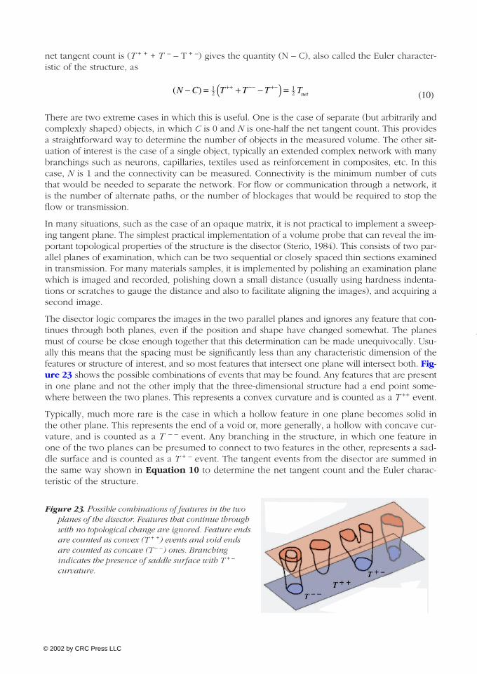
The disector logic compares the images in the two parallel planes and ignores any feature that con-tinues through both planes, even if the position and shape have changed somewhat. The planesmust of course be close enough together that this determination can be made unequivocally. Usu-ally this means that the spacing must be significantly less than any characteristic dimension of thefeatures or structure of interest, and so most features that intersect one plane will intersect both. Fig-ure 23 shows the possible combinations of events that may be found. Any features that are presentin one plane and not the other imply that the three-dimensional structure had a end point some-where between the two planes. This represents a convex curvature and is counted as a T ++ event.

Typically, much more rare is the case in which a hollow feature in one plane becomes solid inthe other plane. This represents the end of a void or, more generally, a hollow with concave cur-vature, and is counted as a T – – event. Any branching in the structure, in which one feature inone of the two planes can be presumed to connect to two features in the other, represents a sad-dle surface and is counted as a T + – event. The tangent events from the disector are summed inthe same way shown in Equation 10 to determine the net tangent count and the Euler charac-teristic of the structure.


( )N C T T T Tnet− = + −( ) =++ −− +−12

12

Figure 23. Possible combinations of features in the twoplanes of the disector. Features that continue throughwith no topological change are ignored. Feature endsare counted as convex (T + +) events and void endsare counted as concave (T – –) ones. Branchingindicates the presence of saddle surface with T + –

curvature.

1142_CH08 pp445 4/26/02 8:58 AM Page 465



Because most of the features seen in the disector images continue through both sections and socontribute no information, it is necessary to examine many pairs of sections, which of course mustbe aligned to compare intersections with the features. When the matrix is transparent and viewedin a confocal microscope, examining and comparing the parallel section planes is straightforward.When conventional serial sections are used, it is attractive to use computer processing to alignand compare the images. The Feature-AND logic described in Chapter 7 is particularly useful in thisregard, to find features that continue through both sections. It is also necessary to sample a largeimage area, well distributed to meet the usual criteria of random, uniform sampling (since the di-sector is a volume probe, isotropy is not an issue).

For opaque matrices, the problems are more severe. Generally it is necessary to prepare a polishedsection, image it, place some fiducial marks on it for reference, and then polish down to somegreater depth in the sample and repeat the process. If the fiducial marks are small pyramidal hard-ness indentations (commonly used to measure hardness of materials), the reduction in their sizeprovides a measure of the distance between the two planes. Aligning and comparing the two im-ages to locate new features can be quite tedious.

Figure 24 shows an example. The specimen is a titanium alloy in which the size of colonies ofWidmanstatten laths is of interest. Each colony is identified by its lath orientation. After one set ofimages was acquired on a metallographically polished plane, the material was polished down a fur-ther 5 µm (as measured from the size change of a microhardness indentation) and additional cor-responding images acquired. In the example, another colony (identified by the red arrow) has ap-peared. From the total number of positive tangent events and the volume sampled by the disector,the mean colony volume was determined.

Anisotropy and gradientsThere is much emphasis above on methods for performing sectioning and applying grids that elim-inate bias in those structures that may not be IUR. Of course, when the specimen meets those cri-teria then any sampling method and grid can be used, but in most cases it is not possible to assume

Figure 24. Scanning electron micrographs of colonies of laths in a titanium alloy (images courtesy Dr. H.Fraser, Dept. of Materials Science and Engineering, Ohio State University, Columbus, OH). The twoimages represent parallel planes with a measured spacing of 5 µm. A new colony (red arrow andoutline) appears in one image, producing a single positive tangent count (T++).

1142_CH08 pp445 4/26/02 8:58 AM Page 466


an IUR structure. Thus, techniques such as vertical sectioning and cycloid grids are used, since theywill provide unbiased results whether the specimen is IUR or not, at the cost of somewhat moreeffort in preparation and measurement.

In some situations, it may be important to actually measure the anisotropy (preferred orientation)in the specimen, or to characterize the nonuniformity (gradients) present in the structure. This re-quires more effort. First, it is usually very important to decide beforehand what kind of anisotropyor gradient is of interest. Sometimes this is known a priori based on the physics of the situation.Deformation of materials in fabrication and the growth of plants typically produce grains or cellsthat are elongated in a known direction, for example. Many physical materials and biological tis-sues have structures that vary markedly near surfaces and outer boundaries, so a gradient in thatdirection may be anticipated. Anisotropy can be qualitatively determined visually, by examining im-ages of planes cut in orthogonal directions, as shown in Figures 25 and 26. It is usually necessaryto examine at least two planes to distinguish the nature of the anisotropy as shown in Figure 27.


Figure 25. Anisotropy inmuscle tissue, visibleas a difference instructure in transverse(b,d) andlongitudinal (a,c)sections.

Figure 26. Anisotropy in rolled steel, shown by microscopicexamination of three orthogonal polished surfaces.

1142_CH08 pp445 4/26/02 8:58 AM Page 467



When there is expectation that directionality is present in the structure, the classic approach is touse grids to measure selectively in different directions. For example, in the case shown in Figure28, the number of intercepts per unit line length (which measures the surface area per unit vol-ume) can be measured in different directions by using a rotated grid of parallel lines. Since eachset of lines measures the projected surface area normal to the line direction, the result shows theanisotropy of surface orientation. Plotting the reciprocal of number of intersections/line length(called the intercept length) as a function of orientation produces a polar (or rose) plot as shownin the figure, which characterizes the mean shape of the grains or cells.

Figure 27. The need to examine at least two orthogonal surfaces to reveal thenature of anisotropy. In the example, the same appearance on one face canresult from different three-dimensional structures.

Figure 28. Characterizinganisotropy: (a) an anisotropic metalgrain structure; (b) the idealized grainboundaries produced bythresholding andskeletonization; (c) measuring the number ofintercepts per unit line lengthin different orientations byrotating a grid of parallellines; (d) the results shown as apolar plot of mean interceptlength.

a b

c d

1142_CH08 pp445 4/26/02 8:58 AM Page 468


Gradients can sometimes be observed by comparing images from different parts of a specimen, butbecause visual judgment of metric properties such as length of boundary lines and area fraction ofa phase is not very reliable it is usually safest to actually perform measurements and compare thedata statistically to find variations. The major problem with characterizing gradients is that they arerarely simple. An apparent change in the number of features per unit area or volume may hide amore significant change in feature size or shape, for example. Figure 29 shows some examples inwhich gradients in size, number, shape and orientation are present. A secondary problem is thatonce the suspected gradient has been identified, a great many samples and fields of view may berequired to obtain adequate statistical precision to properly characterize it.

Figure 30 shows a simple example of the distribution of cell colonies in a petri dish. Are they pref-erentially clustered near the center, or uniformly distributed across the area? By using the methodshown in Chapter 7 to assign a value from the Euclidean distance map (of the area inside the petridish) to each feature, and then plotting the number of features as a function of that value, the plotof count vs. radial distance shown in Figure 31 is obtained. This would appear to show a decreasein the number of features toward the center of the dish; but this is does not correctly represent theactual situation, because it is not the number but the number per unit area that is important, andthere is much more area near the periphery of the dish than near the center. If the distribution ofnumber of features as a function of radius is divided by the number of pixels as a function of ra-dius (which is simply the histogram of the Euclidean distance map), the true variation of numberper unit area is obtained as shown in the figure.

Size distributionsMuch of the contemporary effort in stereological development and research has been concernedwith improved sampling strategies to eliminate bias in cases of non-IUR specimens. There have also


Figure 29. Schematic examplesof gradients in: (a) size; (b) area fraction; (c) shape; (d) orientation.

a b

c d

1142_CH08 pp445 4/26/02 8:58 AM Page 469



been interesting developments in so-called second order stereology that combine results from dif-ferent types of measurements, such as using two different types of grids to probe a structure or twodifferent and independent measurements. One example is to use a point grid to select features formeasurement in proportion to their volume (points are more likely to hit large than small particles).For each particle that is thus selected, a line is drawn (in a random direction) through the selec-tion point to measure the radius from that point to the boundary of the particle.

Figure 32 shows this procedure applied to the white dendritic phase in the image used earlier. Thegrid of points selects locations. For each point that falls onto the phase of interest, a radial line inuniformly randomized directions is drawn to the feature boundary. For convex shapes, the lengthof this line may consist of multiple segments which must be added together. For isotropic structuresor isotropic section planes, the line angles uniformly sample directions. For vertical sectionsthrough potentially anisotropic structures, a set of sine-weighted angles should be used.

The length of each line gives an estimate of particle volume:

(11)

which is independent of particle shape. Averaging this measurement over a surprisingly small num-ber of particles and radius measurements gives an estimate of the volume-weighted mean volume(in other words, the volume-weighted average counts large particles more often than small ones,in proportion to their volume).

A more common way to define a mean volume is on a number-weighted basis, where each parti-cle counts equally. This can be determined by dividing the total volume of the phase by the num-ber of particles. We have already seen how to determine the total volume fraction using a point

Figure 30. Distribution of features within an area (e.g., cellcolonies in a petri dish), with each one labeled accordingto distance from the periphery.

Figure 31. Data from Figure 30. Plot of number and numberper unit area as a function of distance.

V r= π43

3

1142_CH08 pp445 4/26/02 8:58 AM Page 470


count, and the number of particles per unit volume using the disector. Dividing the total by thenumber gives the number-weighted mean volume.

Once both the mean volumes have been determined, they can be combined to determine thestandard deviation of the distribution of particle sizes, independent of particle shape, since forthe conventional number-weighted distribution the variance is given by the difference betweenthe square of the volume-weighted mean volume and the square of the number-weighted meanvolume

(12)

Although this may appear to be a rather esoteric measurement, in fact it gives an important char-acterization of the size distribution of particles or other features that may be present in a solid,which as we have seen are not directly measurable from the size distribution of their intersectionswith a plane section.

Classical stereology (unfolding)Historically, much of classical stereology was concerned with exactly that problem, determining thesize distribution of three-dimensional features when only two-dimensional sections through themwere measurable (Weibel, 1979; Cruz-Orive, 1976, 1983). The classical method used was to as-sume a shape for the particles (i.e., that all of the particles were the same shape, which did not varywith size). The most convenient shape to assume is (of course) a sphere. The distribution of thesizes of circles produced by random sectioning of a sphere can be calculated as shown in Figure33. Knowing the sizes of circles that should be produced if all of the spheres were of the same sizemakes it possible to calculate a matrix of α values that enable solving for the distribution of spheresizes that must have been present in the three-dimensional structure to produce the observed dis-tribution of circle sizes, as shown in Figure 34.

(13)

Other shapes have also been proposed, as a compromise between mathematical ease of calcula-tion and possible realistic modeling of real world shapes. These have included ellipsoids of revo-lution (both oblate and prolate), disks, cylinders, and a wide variety of polyhedra, some of whichcan be assembled to fill space (as real cells and grains do). Tables of alpha coefficients for all


Figure 32. Measuring point-sampled intercepts: (a) an array of grid points,each having a directionassociated with it; (b) applying the grid to theimage from Figure 2 andmeasuring the radial distancefrom those grid points that fallon the phase of interest to theboundary in the chosendirection. Note that, forconvex shapes, the radialdistance is the sum of allportions of the intercept line.

a b

σ2 2 2= −V VV N

N NV i j Asphere i circle j, ,,= ⋅∑α

1142_CH08 pp445 4/26/02 8:58 AM Page 471



these exist and can be rather straightforwardly applied to a measured distribution of the size oftwo-dimensional features viewed on the section plane.

However, there are several critical drawbacks to this approach. First, the ideal shapes do not usu-ally exist. Nuclei are not ideal spheres, cells and grains are not all the same polyhedral shape (infact, the larger ones usually have more faces and edges than smaller ones), precipitate particles inmetals are rarely disks or rods, etc. Knowledge of the shape of the three-dimensional object iscritical to the success of the unfolding method, since the distribution of intersection sizes variesconsiderably with shape (Figure 35 shows an example of cubes vs. spheres). It is very commonto find that size varies with shape, which strongly biases the results. Small errors in the shape as-sumption produce very large errors in the results. For example, the presence of a few irregulari-ties or protrusions on spheres results in many smaller intersection features, which are mis-inter-preted as many small spherical particles.

The second problem is that from a mathematical point of view, the unfolding calculation is ill-posed and unstable. Variations in the distribution of the number of two-dimensional features as afunction of size result from counting statistics. The variations are typically greatest at the end of the

Figure 33. Sectioning asphere at random producesa distribution of circlesizes.

Figure 34. Unfolding the sizedistribution of spheres thatmust have been present toproduce an observeddistribution of circle sizes.The sample is a cast ironcontaining graphitenodules; note that thefeatures are not perfectlycircular, even though asphere model has beenused in the unfolding.

1142_CH08 pp445 4/26/02 8:58 AM Page 472


distribution, for the few largest features which are rarely encountered. But in the unfolding processthese errors are magnified and propagated down to smaller sizes, often resulting in negative num-bers of features in some size classes, and greatly amplifying the statistical uncertainty.

For these reasons, although unfolding was a widely used classical stereological method fordecades, it has fallen out of favor in the last 15–20 years. Instead there has been increased em-phasis on finding unbiased ways to measure structural parameters using more robust tools. Nev-ertheless, in spite of these limitations (or perhaps because their magnitude and effect are not suf-ficiently appreciated), unfolding of size distributions is commonly performed. When the shape ofthe three-dimensional objects is not known, it is common to assume they are simple spheres, evenwhen the observed features are clearly not circles. The argument that this gives some data that canbe compared from one sample to another, even if it is not really accurate, is actually quite wrongand simply betrays the general level of ignorance about the rules and application of stereologicalprocedures.


Figure 35. Size distribution of intercept areasproduced by random sectioning of a sphereand a cube.

1142_CH08 pp445 4/26/02 8:58 AM Page 473


global image measurements - uzh · the science of stereology relates the measurements that can be...

Documents