global illumination of point models - cse.iitb.ac.inrhushabh/aps/aps5/aps5_report.pdf · global...
TRANSCRIPT

Global Illumination of Point Models
Fifth Progress Report
Submitted in partial fulfillment of the requirementsfor the degree of
Ph.D.
by
Rhushabh GoradiaRoll No: 04405002
under the guidance of
Prof. Sharat Chandran
aDepartment of Computer Science and Engineering
Indian Institute of Technology, BombayMumbai
September 30, 2009

1 Motivation and Problem Definition
Figure 1: Grottoes, such as the ones from China and India form a treasure for mankind. If data from the ceilingand the statues are available as point samples, can we capture the inter-reflections?
Photo-realistic computer graphics attempts to match as closely as possible the rendering of a scene with its
actual photograph. Virtual scenes should have a similar property. Of the several techniques that are used to
achieve this goal, physically-based approaches (i.e., those that attempt to simulate the actual physical process
of illumination) provide the most striking results.
My thesis problem is that of producing global illumination (GI) solution for point models. For example, these
three-dimensional point models may be 3D scans of cultural heritage structures (see Figure 1) and we may wish
to view them in a virtual museum under various lighting conditions.
CHALLENGES: The point clouds of interest are not solitary models, but may consist of hard to segment
entities thereby inhibiting a surface reconstruction algorithm that produces meshes. Acquiring 3D point sam-
ples is easy and cheap now but GI solutions are not existent and neither are they cheap. Further, the global
illumination algorithm should handle point models with any of diffuse or specular material properties, there by
capturing all known light reflections, namely, diffuse reflections, specular reflections, specular refractions and
caustics.
PROBLEM DEFINITION: To compute global illumination solution (specular and diffuse) of complex scenes
represented as point models
2 Layout of the report
The report is organized as follows. § 3 enlists the phases to solve my thesis problem along with the progress
status for each phase. It is supported with publications and technical reports in § 4. An introduction to point
models and GI is presented in § 5 and § 6 respectively. We then move on to the details of the algorithms used
1

in each of the enlisted phases. GI effects, in a broad sense, are the result of Diffuse and Specular types of
light reflections and refractions. We give a brief overview of the algorithms used to capture diffuse effects
on point models in § 7. Within the same, § 7.1 presents an introduction to the FMM algorithm for Radiosity
based diffuse global illumination kernel designed for point models. We then discuss the importance of mutual
point-pair visibility for correct global illumination results and the algorithm developed for achieving the same
in § 7.2. Parallel implementations on Graphics Processing Units were used for achieving multi-fold speed-ups
for both the above algorithms as the sequential implementations were very slow and not suited for practical
applications. The GPU-based versions of the same are overviewed in § 7.3. Details pertaining to all the above
algorithms have already been presented in my previous APS reports [Gor07, Gor08].
We then list algorithms, in § 8, which capture specular inter-reflection effects (reflections, refractions, caus-
tics) for point-models. We present algorithms which helps us solving view-dependent, first-object intersection
queries essential for ray-tracing. The ray-tracer and caustics-generator are implemented on the GPU using
CUDA. This work was done in the course of this year. § 10 concludes and outlines a brief summary of my
thesis work.
3 Work Progress
• We compute diffuse inter-reflections using the Fast Multipole Method (FMM) [Gor06] (Done)
• Mutual point-pair visibility queries required for correct diffuse global illumination. We invent Visibility
Maps(V-Maps) to provide an efficient solution [Gor07] [GKCD07] (Done)
• CPU-based implementations of visibility and FMM algorithms were quite time consuming and hence did
not have a high practical usage. Parallel implementation of visibility and FMM algorithms on Graphics
Processing Units(GPUs) using CUDA [CUD] was done so as to achieve multi-fold speedups for gener-
ating the diffuse global illumination solution [GAC08] [Gor08] (Done)
• Inter-reflection effects include both diffuse (Done) and specular effects like reflections, refractions, and
caustics. We present algorithms to solve quickly the view-dependent, first-object intersection visibility
queries for capturing specular reflections. These, when essentially combined with the algorithms for
capturing the diffuse inter-reflections, will give a complete global illumination package for point models.
The algorithms required for achieving these effects are detailed in this report (ONGOING)
4 Publications
1. Visibility Map for Global Illumination in Point Clouds by R. Goradia, A. Kanakanti, S. Chandran and A.
Datta was accepted as an oral paper at Proceedings of ACM SIGGRAPH GRAPHITE, 5th International
2

Conference on Computer Graphics and Interactive Techniques, 2007. It presents our V-map construction
algorithm on the CPU [GKCD07].
2. GPU-based Hierarchical Computation for View Independent Visibility by R. Goradia, P. Ajmera and S.
Chandran was accepted as an oral paper at ICVGIP, Indian Conference on Vision, Graphics and Image
Processing, 2008. This paper details our fast, GPU-based V-map construction algorithm [GAC08].
3. Fast, parallel, GPU-based construction of space filling curves and octrees by P. Ajmera, R. Goradia, S.
Chandran and S. Aluru was accepted as a poster at ACM SIGGRAPH SI3D ’08: Proceedings of the 2008
symposium on Interactive 3D graphics and games, 2008. It presents a GPU-based, parallel octree, and
first-ever parallel SFC construction algorithm [AGCA08].
The following are some technical reports, yet to be published.
• Fast, GPU-based Illumination Maps for Point Models using FMM by R. Goradia, P. Ajmera and S.
Chandran. This work details FMM algorithm for point models to achieve a global illumination solution
and the enhanced, fast version of the same on the GPU.
• GPU-based, fast adaptive octree construction algorithm by R. Goradia, P. Ajmera, S.Chandran and S.
Aluru. It presents two, different, memory-efficient parallel octree construction algorithms on the GPU,
which can be combined with the current GPU-based FMM framework.
• Specular Inter-reflections on Point Models by R. Goradia, S. Kashyap, and S.Chandran. We discuss
algorithms to get a quick answer to first object intersection queries required for capturing caustics and
other specular reflections and refractions during ray-tracing of point models. The ray-tracer and caustics-
generator are implemented on the GPU using CUDA.
3

5 Point Based Modelling and Rendering
Figure 2: Point Model Representation. Explicit structure of points for bunny is visible. Figure on extreme rightshows the same bunny with continuous surface constructed
Point models are nothing but a discrete representation of a continuous surface i.e. we model each point as
a surface sample representation (Fig 2). There is no connectivity information between points. Each point has
certain attributes, for example co-ordinates, normal, reflectance, emmisivity values.
Figure 3: Example of Point Models
In recent years, point-based methods have gained significant interest. In particular their simplicity and total
independence of topology and connectivity make them an immensely powerful and easy-to-use tool for both
modelling and rendering. Directly rendering them without the need for cleanup and tessellation makes for a
huge advantage.
Second, the independence of connectivity and topology allow for applying all kinds of operations to the points
without having to worry about preserving topology or connectivity. This allows for efficiently reducing aliasing
through multi-resolution techniques [PZvBG00, RL00, WS03], which is particularly useful for the currently
observable trend towards more and more complex models: As soon as triangles get smaller than individual
pixels, the rationale behind using triangles vanishes, and points seem to be the more useful primitives. Figure 3
shows some example point based models.
4

6 Global Illumination
Figure 4: Global Illumination. Top Left[KC03]: The ‘Cornell Box’ scene. This image shows local illumination.All surfaces are illuminated solely by the square light source on the ceiling. The ceiling itself does not receiveany illumination. Top Right[KC03]: The Cornell Box scene under a full global illumination solution. Noticethat the ceiling is now lit and the white walls have color bleeding on to them.
Local illumination refers to the process of a light source illuminating a surface through direct interaction.
However, the illuminated surface now itself acts as a light source and propagates light to other surfaces in the
environment. Multiple bounces of light originating from light sources and subsequently reflected throughout
the scene lead to many visible effects such as soft shadows, glossy reflections, caustics and color bleeding. The
whole process of light propagating in an environment is called Global Illumination and to simulate this process
to create photo-realistic images of virtual scenes has been one of the enduring goals of computer graphics.
More formally,
Global illumination algorithms are those which, when determining the light falling on a surface, take into
account not only the light which has taken a path directly from a light source (direct illumination), but also
light which has undergone reflection from other surfaces in the world (indirect illumination).
Because GI effects are natural, we wish to see the effects of Global Illumination (GI) – the simulation of the
physical process of light transport that captures inter-reflections – on point clouds of not just solitary models,
but an environment that consists of such hard to segment entities (Fig. 1). Most computer generated pictures do
not perform GI due to speed limitations (movies are a big exception).
Global Illumination effects are the results of two types of light reflections and refractions, namely Diffuse and
5

Specular.
6.1 Diffuse and Specular Inter-reflections
Diffuse reflection is the reflection of light from an uneven or granular surface such that an incident ray is seem-
ingly reflected at a number of angles. The reflected light will evenly spread over the hemisphere surrounding
the surface (2π steradians) i.e. they reflect light equally in all directions.
Specular reflection, on the other hand, is the perfect, mirror-like reflection of light from a surface, in which
light from a single incoming direction (a ray) is reflected into a single outgoing direction. Such behavior is
described by the law of reflection, which states that the direction of incoming light (the incident ray), and the
direction of outgoing light reflected (the reflected ray) make the same angle with respect to the surface normal,
thus the angle of incidence equals the angle of reflection; this is commonly stated as θi = θr.
The most familiar example of the distinction between specular and diffuse reflection would be matte and
glossy paints as used in home painting. Matte paints have a higher proportion of diffuse reflection, while gloss
paints have a greater part of specular reflection.
Figure 5: Left: Colors transfer (or ”bleed”) from one surface to another, an effect of diffuse inter-reflection.Also notable is the caustic projected on the red wall as light passes through the glass sphere. Right: Reflectionsand refractions due to the specular objects are clearly evident
Due to various specular and diffuse inter-reflections in any scene, various types of global illumination
effects may be produced. Some of these effects are very interesting like color bleeding, soft shadows, specular
highlights and caustics. Color bleeding is the phenomenon in which objects or surfaces are colored by reflection
of colored light from nearby surfaces. It is an effect of diffuse inter-reflection. Specular highlight refers to the
glossy spot which is formed on specular surfaces due to specular reflections. A caustic is the envelope of light
rays reflected or refracted by a curved surface or object, or the projection of that envelope of rays on another
6

surface. Light coming from the light source, being specularly reflected one or more times before being diffusely
reflected in the direction of the eye, is the path traveled by light when creating caustics. Figure 5 shows color
bleeding and specular inter-reflections including caustics.
Radiosity and Ray-Tracing are two basic global illumination algorithms used for diffuse and specular effects
generation (respectively). We compute a radiosity based diffuse solution using the Fast Multipole Method.
We will study the behavior of light paths w.r.t the diffuse and specular objects in the scene and accordingly pace
ourselves with the algorithms required to produce GI effects in such a scene.
7 Diffuse Global IlluminationDiffuse Interactions
Fifth Annual Progress Seminar, 2009 Rhushabh Goradia, Sharat Chandran
L
Source emits light inall directions
Diffuse Interactions
Fifth Annual Progress Seminar, 2009 Rhushabh Goradia, Sharat Chandran
L
LD
Diffuse BRDF High Absorption
Diffuse Interactions
Fifth Annual Progress Seminar, 2009 Rhushabh Goradia, Sharat Chandran
L
LD
LDD/LD+ path
Figure 6: Example showing the behavior of light w.r.t the diffuse objects. The light source emits light in allthe directions (figure on the extreme left). We trace one of those rays which hits the diffuse back wall. Themajority of light energy gets absorbed, and the remaining is reflected in all hemispherical direction (figure inthe middle). One such ray goes and hits another wall. Thus the path travelled here is LDD or in all generalityLD+
To understand the diffuse GI effects, we need to understand the paths light takes up in the scene consisting
of purely diffuse objects. Fig. 6 shows such a scene, where the room and the spheres are diffuse objects. As we
can understand, the light source emits light in all directions. We trace one of those rays. It hits a diffuse surface,
and majority of it gets absorbed. The remaining small portion of light energy is reflected in all hemispherical
direction (property of diffuse B.R.D.F). One such ray goes and hits another wall. Thus the path travelled here
is LDD (light to diffuse, diffuse to diffuse) or in all generality LD+. To capture all such interactions is an N2
problem, since each point in the model (with diffuse properties) might contribute whatever energy it receives
to every other point in the model. However, N in point models is very large, in hundreds of thousands, making
a N2 solution impractical to implement. We try to solve this seemingly irreducible complexity problem using
the Fast Multipole Method in O(N) time.
7

7.1 FMM based Diffuse Global illumination
Diffuse global illumination requires the computation of pairwise interactions among each of the surface ele-
ments (points) in the given data (usually of order > 106) and thus is a N-body problem. We use the technique
of the Fast Multipole Method, to capture diffuse inter-reflections, which is a N-body solver algorithm and
also starts with points as primitives. Thus my problem of capturing diffuse effects naturally fits in the FMM
framework. The FMM attempts to reduce O(N2) seemingly irreducible complexity to O(N + M) or even
O(N logN +M) and hence achieves good speeds. Three main insights that make this possible are:
1. Factorization of the kernel into source and receiver terms
2. Most application domains do not require that the function f be calculated at very high accuracy.
3. FMM follows a hierarchical structure (Octrees)
7.2 Visibility between point pairs
Figure 7: Example showing importance of visibility calculations between points [GKCD07]
Computing a mutual visibility solution for point pairs is a major, necessary step for achieving correct
diffuse reflection results. For example, in Fig. 7, shadows wouldn’t have been possible if there wasn’t any
visibility information. Thus, an important aspect of capturing the radiance is an object space view-independent
knowledge of visibility between point pairs.Visibility calculation between point pairs is essential as a point
receives energy from other point only if it is visible to that point. But its easier said than done. Visibility between
8

point pairs is an N3 problem, as the visibility between two points depends on all other points in the scene.
Further, its complicated in our case as our input data set is a point based model with no connectivity information.
Thus, we do not have knowledge of any intervening surfaces occluding a pair of points. Theoretically, it is
therefore impossible to determine exact visibility between a pair of points. We, thus, restrict ourselves to
approximate visibility.
We construct a V-map on the given scene to provide a view-independent visibility solution for global illumi-
nation for point models ( [GKCD07] [Gor07]). The basic idea is to partition the points in the form of an octree.
When large portions of a scene are mutually visible from other portions, a visibility link is set so that groups of
points (instead of single points) may be considered in discovering the precise geometry-dependent illumination
interaction. Ray shooting and visibility queries can also be answered in sub-linear time using this data structure.
Details of the above mentioned algorithms are available in [Gor07].
7.3 GPU-based FMM and V-Map Construction Algorithms
CPU-based sequential implementations of FMM and V-map construction algorithms are quite time consum-
ing and hence do not have a high practical usage. Parallel implementation of V-map construction and FMM
algorithms on Graphics Processing Units(GPUs) using CUDA [CUD] programming environment was then
performed so as to achieve multi-fold speedups for generating the diffuse global illumination solution. The
following paragraph gives an overview of how this algorithm is structured (Details for the same are available in
[Gor08]).
FMM algorithm, used for solving my problem of diffuse global illumination for point models, consists of the
following five phases:
1. Octree Construction
2. Generating interaction lists
3. Determine visibility between octree nodes (where our V-map is applied). Visible links here determine
the paths of light energy transfers between octree nodes.
4. Upward Pass
5. Downward Pass and Final Summation
Our parallel FMM algorithm specifically solves the last two phases (Upward pass, Downward pass and Final
summation stage) on the GPU. These phases are the ones which take more than 97% of the run time (not taking
9

visibility phase into account). Hence we first implemented these two stages on the GPU while the Octree
Construction and Interaction List Construction stages were performed on the CPU. We assume, as a part of
pre-processing step, that we have been given an octree constructed for the input 3D model along with the
interactions lists for each of the octree nodes (containing only visible nodes). The octree can be constructed on
the CPU or on the GPU while the interaction lists construction happens on the CPU. Visibility between octree
nodes is determined by using a CPU-GPU combo algorithm detailed in [GAC08].
7.4 GPU-based Parallel Octree Construction for FMM
The FMM enables an answer to the N-body problem of GI to be evaluated in just O(N) operations. One of
the main insight that makes this possible is the underlying hierarchical structure of the Octree. Three different
parallel octree construction algorithms were designed so as to be used with the parallel FMM-GPU framework.
The algorithms are detailed in [Gor08].
Work on achieving fast, GPU-based diffuse global illumination solver for point models using parallel
octrees, V-map and FMM algorithms was completed last year [Gor08]. However, to capture all the GI
effects (like glossy reflections, refractions and caustics) we require a specular-effect solver as well. We
discuss, in section § 8 how we handle the specular effects like caustics, reflections and refractions with
the help of a fast, first-object intersection solver. The ray-tracer and caustics-generator are implemented
on the GPU using CUDA.
8 Specular Inter-reflections
After having seen the algorithms and techniques for computing diffuse global illumination on point models, let
us now focus on computing specular effects (reflections and refractions) including caustics for the point models.
These, combined with already calculated diffuse illumination gives the user a complete global illumination
solution for point models.
First we would like to study the behavior of light paths in a scene comprising of both the diffuse and specular
objects. In addition we should also have a look at what changes need to be made in our diffuse GI algorithms
for such scenes. We then look into the details of how and what all specular effects to achieve.
8.1 Light Paths in a Diffuse-Specular Scene
Consider the scene given in Fig. 8. It shows two specular spheres placed in a room with diffuse walls. Light
emitted from the light source on the ceiling can take up 4 different paths, viz, LDD, LSD, LDS and LSS
(l-light, D-diffuse, S-specular). The figure shows all 4 different paths. We want to capture all these paths to get
10

Diffuse-Specular Scene
Fifth Annual Progress Seminar, 2009 Rhushabh Goradia, Sharat Chandran
L
LD
4 different paths takenup by light
LDD/LD+
LSD/LS+D LDS/LD+S+D LSS
Diffuse-Specular Scene
Fifth Annual Progress Seminar, 2009 Rhushabh Goradia, Sharat Chandran
L
4 different paths takenup by light
LDD/LD+
LSD/LS+D LDS/LD+S+D LSS LS
LSD
Light received through LSD path must be distributed during diffuse inter-reflections
Pre-process and Store
LS+D -- Caustics!Diffuse-Specular Scene
Fifth Annual Progress Seminar, 2009 Rhushabh Goradia, Sharat Chandran
L
LD
4 different paths takenup by light
LDD/LD+
LSD/LS+D LDS/LD+S+D LSS
LS+D similar to LD+S+D
Energy transfer too low !
Ignore !
Diffuse-Specular Scene
Fifth Annual Progress Seminar, 2009 Rhushabh Goradia, Sharat Chandran
L
4 different paths takenup by light
LDD/LD+
LSD/LS+D LDS/LD+S+D LSS LS
LSS
LSS similar to LS+D
Pre-processed Caustics!
Figure 8: Example showing the behavior of light w.r.t the diffuse and specular objects. The light emitted cantake up 4 different paths, viz LDD, LSD, LDS, LSS. Figures show all the 4 paths.
both the diffuse and specular GI effects in the given scene.
As we have seen in § 7, to capture the diffuse effects we need to take care of the LDD paths taken by the light.
However, now the problem gets a bit more complicated since the new path LSD also deposits energy on the
diffuse component in the scene. Further, the deposited energy must be absorbed and then distributed equally
in all the hemispherical directions, similar to what happens in LDD paths. Thus, to capture the LSD or in
general LS+D energy transfers correctly, we pre-process these transfers and store the transferred energy at the
corresponding diffuse point objects. We then apply our FMM-based radiosity approach, also taking this stored
energy due to LS+D paths into account, to take care of the LDD paths.
11

Diffuse-Specular Scene
Fifth Annual Progress Seminar, 2009 Rhushabh Goradia, Sharat Chandran
L
L
Diffuse case
Specular case
A
A
B
B
During FMM transfers, surfaces A and B will still be invisible to L !
Diffuse-Specular Scene
Fifth Annual Progress Seminar, 2009 Rhushabh Goradia, Sharat Chandran
L
L
Diffuse case
Specular case
A
A
B
B
During FMM transfers, surfaces A and B will still be invisible to L !Figure 9: Figure on left shows surfaces A and B being occluded from the light source by an opaque sphere.A and B never receive any light. Figure on the right shows a similar scene setting except the sphere is nowa transparent, refractive one. LSD path transfer energy from the light source to A, while the LDD paththereafter, transfers the stored energy at A to B.
Figure 9 shows one such example. Both surfaces A and B are invisible to the light source due to the
occluding sphere. In the first case (figure on left), A and B both will be in shadow due to opaque sphere
occlusion. On the other hand, in the second case, since the sphere is a refractive and transparent, we handle the
transfer of light via LSD path first, depositing some energy at A. We then call the FMM procedure to take care
of LDD paths, thereby transferring the stored energy from A to B. Note that during FMM none of the energy
will be transferred from the light source to either A or B.
Since the energy transfers between specular and diffuse have already been pre-processed, we must now make
sure these transfers don’t happen while performing FMM for LDD path interactions. Thus, while performing
FMM, neither is energy contributed from specular components in the scene nor is energy distributed to any
specular components in the scene. V-Map construction remains the same.
In case the light takes up LDS path or in general LD+S+D path, we simply ignore its contribution. Since the
ray of light emitted from the source first hits the diffuse object, the energy emitted from the diffuse object for
the secondary ray, in the direction of some specular object, is very negligible. Such paths are hence not taken
care of. LSS paths are nothing but LS+D paths and are handled in a similar fashion.
Thus, we need to capture the LS+D paths before the LDD paths to take care of specular interactions with the
diffuse objects. This LS+D paths taken up by the light give rise to one of our desired effects: The Caustics!
Note that whatever light paths we have studied so far are view-independent i.e. the effects captured by these
paths remain the same irrespective of the the viewing co-ordinates and angles. However, many specular effects
of reflections and refractions are view-dependent. To capture these effects from our specific view, we need to
trace rays, now not from the light source, but from our eye/camera. This backward tracing of ray has a common
name in graphics industry, Ray-Tracing
12

8.2 Ray-Trace Rendering
Any ray-tracing algorithm starts by defining a camera (or ray origin), ray directions and a view-plane (refer
Fig. 10).
View Plane
Eye/Camera
Diffuse Splat
Specular Reflective Splat
Specular Reflective Splat
Specular Refractive Splat
Figure 10: Ray-Tracing situation. The view plane is a grid of pixels, and a ray (or multiple rays) is sent througheach pixel to find object intersections. It recurses till it finds a diffuse surface or bounces more than the pre-defined limit. The color of the pixel is addition of all colors at the intersection point of the object the ray hashit along its path
Ray tracing is so named because it tries to simulate the path that light rays take as they bounce around
within the world - they are traced through the scene. The view plane is divided into a grid of pixels and a
ray (or multiple rays in case of super-sampling) is sent through every pixel into the scene. Our objective is
to determine the color of each pixel as the ray traverses the scene undergoing reflections and refractions as it
intersects the scene objects.
This pass of ray-Tracing is performed after we have captured and stored all the view-independent effects. Thus
while we trace the ray, the path taken is either ES+D or ED (E-Eye). Whenever a ray hits a diffuse surface,
either directly from the eye or after multiple bounces from the specular objects, the value stored at that diffuse
intersection object is read back. This value is nothing but the contributions at that intersecting object from
the LS+D and LD+ paths captured previously. To summarize, to get complete GI effects, we consider the
following path LS ∗DS ∗ E.
After having known now what problem we are trying to solve, let us see how we capture these light paths and
eventually the specular effects.
13

8.3 Previous Work: Specular Effects on Point Models
Attempts have been made to get these effects. Schaufler [SJ00] was the first to propose a ray-tracing technique
for point clouds. Their idea is based on sending out rays with certain width which can geometrically be de-
scribed as cylinders. The intersection detection is performed by determining the points of the point cloud that
lie within such a cylinder followed by calculating the ray-surface intersection point as distance-weighted aver-
age of the locations of these points. The normal information at the intersection point is determined using the
same weighted averaging. This approach does not handle varying point density within the point cloud. More-
over, the surface generation is view-dependent, which may lead to artifacts during animations. Wand [WS03]
introduced a similar concept by replacing the cylinders with cones, but they started with triangular models as
their input instead of point models. Adamson [AA03] proposed a method for ray-tracing point-set surfaces but
was computationally too expensive, the running times being in several hours. Wald [WS05] then described a
framework for interactive ray-tracing of point models based on a combination of an implicit surface represen-
tation, an efficient surface intersection algorithm and a specifically designed acceleration structure. However,
implicit surface calculation was too expensive and hence they used ray-tracing only for shadow computations.
Also, the actual shading was performed only by a local shading model. Thus, transparency and mirroring re-
flections were not modelled. Linsen [LMR07] recently introduced a method of Splat-Based Ray-Tracing for
Point Models handling the shadow, reflections and refraction effects efficiently. However, they did not consider
rendering caustics effects in their algorithm.
Our proposed method successfully gets all the desired specular effects (reflections, refractions and caustics)
along with producing a time efficient algorithm for the same. We also fuse it with the diffuse illumination
algorithm to give a complete global illumination solution.
Our proposed algorithm follow the Photon Mapping (for polygonal models) [Jen96] strategy closely. Therefore,
we start by giving a brief overview of this technique and then follow up with our own algorithms for achieving
specular effects.
8.4 Photon Mapping
The global illumination algorithm based on photon maps is a two-pass method. The first pass builds the photon
map by emitting photons from the light sources into the scene and storing them in a photon-map data structure
when they hit non-specular objects. There are two types of photon maps viz.
• Caustic Photon Map: contains photons that have been through at least one specular reflection before
hitting a diffuse surface: LS+D.
• Global Photon Map: an approximate representation of the global illumination solution for the scene for
14

all diffuse surfaces: L(S|D)∗D
(a) (b)
Figure 11: Figure 11(a) shows the construction of the caustics photon map with a dense distribution of pho-tons,and Figure 11(b) shows the construction of the global photon map with a more coarse distribution ofphotons.
The construction of the photon maps is most easily achieved by using two separate photon tracing steps in
order to build the caustics photon map and the global photon map. This is illustrated in Figure 11 for a simple
test scene with a glass sphere and 2 diffuse walls. Figure 11(a) shows the construction of the caustics photon
map with a dense distribution of photons,and Figure 11(b) shows the construction of the global photon map
with a more coarse distribution of photons.
The second pass, the rendering pass, uses statistical techniques on the photon map to extract information about
incoming flux and reflected radiance at any point in the scene. The photon map is decoupled from the geometric
representation of the scene. This is a key feature of the algorithm, making it capable of simulating global
illumination in complex scenes containing millions of triangles, instanced geometry, and complex procedurally
defined objects.
In the rendering pass, the photon map is a static data structure that is used to compute estimates of the incoming
flux and the reflected radiance at many points in the scene. To do this it is necessary to locate the nearest
photons in the photon map. This is an operation that is done extremely often, and it is therefore a good idea to
optimize the representation of the photon map before the rendering pass such that finding the nearest photons
is as fast as possible.
The data structure should be compact and at the same time allow for fast nearest neighbor searching. It should
also be able to handle highly non-uniform distributions this is very often the case in the caustics photon map.
A natural candidate that handles these requirements is a kd-tree.
15

8.5 Our Approach
We now present our algorithm to generate specular effects for point models. We apply a similar path/phases as
seen in photon mapping algorithm, but change some basic algorithms used to generate those specular effects.
8.5.1 Octree Creation: Changed
The octree we use for diffuse global illumination is constructed in a top-down fashion. It goes on sub-dividing
a node into 8 parts until each leaf has maximum of k points inside it (eg. Construct an octree till each leaf
has max. of 10 points). If k here is pretty small, we may well assume that points belonging to a particular
leaf belong to a same surface. Now we change this construction algorithm slightly (Fig. 12) by modifying
Root
D D D D D DS S S S SLeaves
D – Leaf containing points with diffuse propertiesS – Leaf containing points with specular properties
An internal node can contain both diffuse and specular points in its subtree
Figure 12: Modified octree for a scene containing both diffuse and specular points
the termination criteria, so as to accommodate specular points too. We now terminate an octree construction
process if a particular leaf has less than k points and all the points in a particular leaf are either specular or
diffuse. Thus, a leaf cannot have both specular and diffuse points inside it. We term a leaf containing just
diffuse points as a diffuse leaf and the leaf containing specular points as a specular leaf.
8.5.2 Caustics on Point Models: LS+D path
This phase achieves the specular view-independent effect of caustics. It takes the octree constructed on point
model as input along with the respective V-Map. The output of this phase is sent as an input to the FMM
algorithm (LDD paths) to consider the diffuse interactions.
The caustic effect generation algorithm consists of following phases:
• Generate caustic photons at the light source
16

• Trace photons (LS+D) in the scene and deposit the photon on a diffuse surface after at least one hit from
a specular surface. Every point in the model has some radius associated with itself (radius is an input
parameter) which gives an approximate local surface area the point covers. We coin these points with
their associated radius as splats. We thus, use a Ray-Splat intersection algorithm to find the intersection
of photons with these splats.
• Form a kd-tree on the caustic photon map for fast search of photons during ray-tracing. After tracing
photons through the scene, we need to store them when they hit the diffuse surface (LS+D). Note that
the photons are only stored when they hit diffuse surfaces (or, more precisely, non-specular surfaces). The
reason is that storing photons on specular surfaces does not give any useful information: the probability of
having a matching incoming photon from the specular direction is zero, so if we want to render accurate
specular reflections the best way is to trace a ray in the mirror direction using standard ray tracing. For
all other photon-surface interactions, photon-data is stored in a global data structure, the caustic photon
map. Given the caustic photon map, we can proceed with the rendering pass. The photon map is view
independent, and therefore a single photon map constructured for an environment can be utilized to
render the scene from any desired view. It can thus be viewed as a pre-computation step.
• Render using ray-tracing (view-dependent)
The path taken by photons to construct a caustic map is LS+D. Note that we do not continue tracing the
photon after it hits the diffuse surface (the path traced is LS+D and NOT LS+D+), as the contribution of
that photon drastically reduces, knowing that diffuse surface have a high enough absorption coefficient and it
sends equal output energy in all hemispherical directions. Thus, the energy of the photon sent in one of the
thousand hemispherical directions is very very low, and hence ignored. For the same reasons, we also do not
send photons from the light source onto the diffuse splats to aid in generating caustic effects.
8.5.3 Photon Generation
The photons emitted from a light source should have a distribution corresponding to the distribution of emis-
sive power of the light source. If the power of the light is Plight and the number of emitted photons is ne, the
energy of each emitted photon is
Pphoton = Plight/ne.
For the light source, we define the maximum number of photons (ne) it can contribute (eg.400000). Since
the caustic effects generated on a diffuse surface are caused after at least one specular hit by the ray originating
17

from the light source, we can safely send rays from the light source only to the “specular” leaf-nodes in the
octree visible to the light source and the light source’s ancestors.
The visible list (part of the V-Map) of the light source (and its ancestors) assists in sending rays only to visible
specular leaf nodes. This accounts for a lot of time-saving, as we don’t have to send packets of rays in every
direction from the light source searching for the probable caustic generators (as in [DBMS02] [GWS04]).
r
c
-- Distance from centroid of the disk to center of the splat
-- Radius of the splat
If “D” is the distance from centroid of the disk to center of a splat plus the splat’s radius, the radius “r” of the disk is set to the “maximum D”
Figure 13: Radius of an average disk (of a particular leaf node) is equal to the maximum “d”, where “d” is thedistance from the center of the disk to the splat’s center plus the radius of that splat
Moving further, for a particular specular leaf nodeA visible to the light source, we need to know how many
photons to shoot in the direction of A. As we know, every leaf node has an average disk D [Gor07] with its
center being the centroid of the points in the leaf and radius r (Fig. 13) equal to the maximum “d”, where “d”
is the distance from the center of the disk to the splat’s center plus the radius of that splat. Thus to find how
many photons to shoot in the direction of node A, we find the solid angle subtended by this average disk D of
A from the light source (Fig. 14).
4π is the total solid angle for a light source. We find the percentage of the total area that is covered by the disk
of A, when we project it onto a unit sphere surrounding the light source. This multiplied by the total number
of photons(ne) gives number of photons to shoot at this node.
number Of Photons = ne ∗ solidAngle(A)/(4π)
A solid angle subtended at a point is given by,
SolidAngle = (Area covered× cosθ)/d2
where d is the distance between the object and the point which subtends the solid angle, and cosθ gives the
inclination of surface towards that point.
18

Light Source
n
rc
Unit Sphere around the light Source
Subtended Solid Angle by the average disk of a node with centroid “c”, radius “r” and average normal “n”
Figure 14: Solid Angle subtended by an average disk of some specular leaf node around the light source. Itgives you an approximate area covered by the node and determines the number of photos to be sent in thatparticular direction
Referring Fig. 14, Let d be the distance between the light source point and the node A’s centroid and Dist
be the distance vector (specifically d = ‖Dist‖). Let n be the average normal of the specular leaf A. The dot
product DP between this distance vector Dist and the cell’s average normal n tells us how much of the cell’s
surface is facing the given light source point.
Area covered by average disk of A is πr2. Thus the solid angle subtended by A is
SolidAngle node A = (πr2 ×DP )/d2
Once we know the solid angle, we know that some x photons needs to be shot in the direction of A. Leaf
A may well have several points inside it and each point in turn has a splat with some radius associated with it.
So, next we find how many photons must be sent to each splat within leaf A. If NP are the number of points
in A, then we send
PPS = x/NP photons per splat
where PPS = photons per splat. The remainder of photons i.e. x%NP are distributed randomly to splats in
A. Thus there will be some splats in A receiving 1 extra photon as compared to other splats.
After knowing PPS for every splat in A, we need to know the photon-hit locations on a particular splat.
Uniform photon-hit grids on a splat will not give good results as it generates artifacts in caustic effects. Hence,
we require a random sampling on each disk, the number of random points generated being equal to PPS for
19

that splat. Any good random number generator can be used for the same.
Thus we now know where to send the photons and how many photons to send in each particular direction from
the light source. The generation of photons at the light sources, and sending them to the visible specular
nodes, is done in parallel on the GPUs, i.e. each thread generates one photon and sends it to the respective
visible specular node. This completes the photon generation and primary ray trace ,using the visible list, from
the light source.
8.5.4 Photon Tracing
Once the photon has been emitted from the light source, we directly place the photon on the splats of some
specular leaf A without actually tracing through the octree with the help of visible list of the light source node
and its ancestors. On hitting a specular leaf, a photon is either transmitted (refracted) or reflected depending on
the material properties of the splat it intersects.1 A photon either reflects or refracts. Depending on whether it
reflects or refracts, a new ray direction for the photon is chosen and the photon is sent out in that direction.
Figure 15: A secondary ray (in brown) is generated in the green leaf. To find the first object of intersectionalong the ray, we need to get to the red leaf next to the green one. We find the intersection point of the ray withthe green leaf, on the plane through which the ray exits (shown in glow), increment along the ray by ∆, and thenew point i. We now traverse from the root downwards, to find which leaf contains point i. We eventually landup at the red leaf.
We now need to trace this refracted or reflected photon, along the ray-direction, through the octree, until it
hits another diffuse or specular object. We start by finding the next octree leaf along the ray-direction. To find
this next leaf, we need to find the intersection point on the plane of the current leaf from where the ray exits,
increment by ∆ along the ray direction from the intersection point and find the leaf containing this new point
(Fig. 15). We provide a fast method to find this containing leaf in § 8.5.11.
If the rays hits a filled leaf cell of the octree, intersection of the ray with all splats stored within that cell is
checked for. If the ray does not intersect any of the splats stored in that cell or if the cell is empty, the algorithm1Note that some part of a photon can be reflected and some be refracted at the same time, say with a glossy translucent splat, but
such cases are a part of future work.
20

proceeds with the adjacent cell in the direction of the ray. If the ray intersects a specular splat stored in the
current cell, it computes the precise intersection point and generates the new reflected/refracted ray. If the ray
hits multiple splats stored in the current cell, the algorithm computes the intersection points and pick the most
appropriate one. On the other hand, if the ray hits a diffuse splat, it deposits the caustic photon energy on that
splat. The above algorithm thus stops when we reach a diffuse surface and deposit the photon there.
We use the parallel compute capabilities of the GPU to trace photons. It traces multiple photons at the
same time in the scene. We use CUDA programming environment to implement the above algorithms.
8.5.5 Normal Field Generation
0Dj-1 1
uj
cj
nl
pl
pi
ni
Figure 16: Generation of normal field (in green) over disk Dj from normals at splats covered by the averagedisk Dj . Normal field is generated using local parameters (u, v) ∈ [−1, 1] × [−1, 1] over the disk’s planespanned by vectors uj and vj orthogonal to normal nj = ni. The normal of the normal field at center point cjmay differ from ni
When a ray intersects a splat, the new reflected or refracted direction is calculated using the normal of the
intersected splat. Thus normals at splats play a pivotal role in deciding the directions of reflected/refracted rays.
We thus pre-process (during octree construction) and store for every splat a uniformly varying normal field
which gives an accurate normal at any point of intersection on the splat.
Splats in their general form define a piece-wise constant surface. In particular, each splat has exactly one
surface normal assigned to it. Assuming that the point cloud was obtained by scanning a smooth surface,
the application of the rendering technique should result in the display of a smoothly varying surface. Since
ray tracing is based on casting rays, whose directions depend on the surface normals, there’s a need to define
smoothly varying normals over the entire surface of each splat. The normals at each point are used to determine
a smoothly varying normal field defined over a local parameter space of the splat. It can be beneficial to
consider further surrounding points and their normals for the normal field computations. Details on the normal
21

field generation [LMR07] are presented below.
In order to generate a smooth-looking visualization of a surface with a piece-wise constant representation,
there is a need to smoothly (e. g. linearly) interpolate the normals over the surface before locally applying the
light and shading model. Since we do not have connectivity information for our splats, we cannot interpolate
between the normals of neighbored splats. Instead, we need to generate a linearly changing normal field within
each splat. The normal fields of adjacent points should approximately have the same interpolated normal where
the splats meet or intersect.
Since we have an average disk representing all points in a leaf, we generate the smooth varying normal field
on this disk (refer Fig. 16).
Let Dj = (cj , nj , rj) be one of the disks. cj represents the centroid of the node (center of the disk), nj repre-
sents the average normal generated by using splat’s normals, belonging to that node and rj represents the radius
of the disk. In order to define a linearly changing normal field over the disk, we use a local parameterization
on the disk. Let uj be a vector orthogonal to the normal vector nj and vj be defined as vj = njxuj . Moreover,
let ‖uj‖ = ‖vj‖ = rj . The orthogonal vectors uj and vj span the plane that contains the disk Dj . A local
parameterization of the disk is given by
(u, v) 7→ cj + uuj + vvj
with (u, v) ∈ <2 and u2 + v2 ≤ 1. The origin of the local 2D coordinate system is the center of the disk Dj .
Using this local parameterization, a linearly changing normal field nj(u, v) for disk is defined Dj by
nj(u, v) = −→n j + uνjuj + vωjvj
The vector −→n j describes the normal direction in the disks center. It is tilted along the disk with respect to the
yet to be determined factors νj , ωj ∈ <. Figure 16 illustrates the idea.
To determine the tilting factors νj and ωj is exploited the fact that the normal directions are known at the points
of point cloud P that are covered by the average disk. Let pl be one of these points. pl is projected onto the
disk, local coordinates (ul, vl) of pl are determined, and the following equation is derived
nl = −→n j + ulνjuj + vlωjvj
where nl denotes the surface normal in pl. Proceeding analogously for all other points out of P covered by
the disk Dj , a system of linear equations is obtained with unknown variables νj and ωj. Since the system is
over-determined, it can only be solved approximately to get the values of νj and ωj.
8.5.6 Ray Splat Intersection
When a ray hits a node, we check for its intersection with individual splats. We find the splat with nearest
intersection. If the splat is a specular one, we use the normal field of the average disk to get the appropriate
22

i
ns
cs
ncs
Average disk of a node with center “c”
Splat ‘s’
Sj Sj+1
i
i+1
i
ns
cs
ncs
Average disk of a node with center “c”
Splat ‘s’
SjSj+1
i
i+1
Figure 17: (a) When the ray R hits splat S, we do not return the splat’s normal ns. Instead we get the normalat the intersection point i from the normal field generated over that average disk (with center c) and return theinterpolated normal ncs. (b) Ray R intersects splat Sj at point i and is reflected. The reflected ray R
′intersects
splat Sj+1 at point i+ 1. Since splats Sj and Sj+1 are over-lapping, intersection point i+ 1 should be ignored.This behavior is achieved by not considering intersection points within an ∆ neighborhood of i. The dottedcircle in red with center i and radius ∆ shows this region
normal at the intersection point. Note that we perform intersection of the ray with individual splats, but use
the normal field generated on the average disk to get the appropriate normal at the point of intersection. This
assumes the points belonging to the same leaf belong to the same surface (refer Fig. 17(a)). Further, when a
splat Sj+1, the ray intersects, is very close (at a ∆ distance) to the splat Sj the ray has originated from, we
ignore that intersection assuming the intersected splat Sj+1 belongs to the same surface as the origin splat Sj
(refer Fig. 17(b)).
Once the ray hits a specular splat, we need to calculate the reflected or the refracted ray (refer Fig. 18). Let−→i be the incident ray entering the node. Say it intersects a splat i. Let θi be the angle between the normal n
at the intersection point (derived from the normal field of that node) and the incident ray−→i . If the ray reflects,
then let −→r be the new reflected ray. If it refracts, then let−→t be the new refracted/transmitted ray. Assume η1
to be the index of refraction of the medium the incident ray enters from and η2 is the index of refraction of the
intersecting splat. θt is the angle between the new refracted ray and the inverted normal n.
We now calculate the new reflected and the refracted direction for the ray using the following equations:
−→r =−→i − 2cosθi−→n )
−→t = η1
η2
−→i − (η1η2 cosθi +
√1− sin2θt)−→n
with,
cosθi =−→i · −→n
23

Surface Boundary
i
t
r
i r
t
1
2
n
Figure 18: An example showing incident, reflected and transmitted rays
Surface Boundary
i
t
1
2
n
Case of Total Internal Reflection. Instead of incident ray “i” getting transmitted/refracted to ray “t”, it is reflected
TOTAL INTERNAL REFLECTION
Figure 19: The highlighted incident ray is reflected instead of being transmitted. It is a case of total internalreflection
sin2θt = (η1η2 )2(1− cos2θi)
In case of refraction, there’s a condition that limits the range of incoming angles θi. Outside this range, the
24

refracted direction vector does not exists (Fig. 19). Hence there is no transmission. This is called total internal
reflection. The condition is:
sin2θt ≤ 1
It can only happen if one goes from a denser material to a less dense material (e.g. glass to air). This is
because sin2θt can become greater than one if η1η2 > 1.
8.5.7 Photon Storing
While ray-trace rendering, a ray may hit any point in the scene. To know whether a caustic has been formed at
that point, we need to locate the nearest caustic photons stored in the photon map. This is an operation that is
done extremely often, and it is therefore a good idea to optimize the representation of the photon map before
the rendering pass such that finding the nearest caustic photons is as fast as possible.
The data structure should be compact and at the same time allow for fast nearest neighbor searching. It should
also be able to handle highly non-uniform distributions this is very often the case in the caustics photon map.
A natural candidate that handles these requirements is a kd-tree. Details on how to construct and search in a
kd-tree are available at [Wikb]. We use the ANN:A Library for Approximate Near neighbor Search [MA] for
constructing and searching through the kd-tree.
Discussion: To summarize, we have seen how to generate the caustic photons, how many to send in the desired
direction, with what intensity, trace them through the scene and finally deposit them on the diffuse surface.
We form a kd-tree on the deposited caustic photons, thereby aiding fast retrieval of the same while ray-tracing.
Further, we generate, trace, and store each caustic photon in parallel using GPU (with CUDA) to achieve speed-
ups in the caustic generation process.
Let us know look into some details of how we perform ray-trace rendering of the given point model scene.
§ 8.5.8 gives an overview of ray-tracing in general and how our algorithm fits into the ray-tracing framework.
§ 8.5.9 extends the ray-tracing algorithm of § 8.5.8 to CUDA based GPUs to provide a fast, close-to interactive
ray-tracer.
8.5.8 Ray-Trace Rendering using Octrees
This section gives insights on how we trace the rays from the view-dependent plane through the octree to get
to the first object of intersection. As we know, any ray-tracing algorithm starts by defining a camera (or ray
origin), ray directions and a view-plane (refer Fig. 10).
The first step of ray-tracing is to generate primary rays from the camera and trace them in the scene till they
intersect an object. As in our case, we divide the scene into an octree. The steps on how we trace the primary
ray are presented below.
25

View Plane
Eye/Camera
i
i
-- Delta increment to the ray
i – Find leaf containing intersection point “i”. If empty
(node highlighted in red) , proceed to the next node along the ray direction ( node highlighted in blue) , else, do ray-splat intersections (node highlighted in green)
i+1
i+1
i
Figure 20: Primary rays are sent from the camera into the scene. To compute the intersection of the ray withthe octree, a ray-box test is performed. The intersection point is incremented by ∆ and the leaf is searchedwhich contains this intersection point (done by traversing down from the root node). If the ray has hit an emptyoctree node, it advances to the next node in the ray direction, else it computes ray-splat intersections with thesplats in the filled leaf node
1. Check if the ray (for each pixel) intersects the octree. We perform this by a ray-box intersection test,
assuming the root of the octree as a cube. If the ray does not intersect, color the pixel to the background
color
2. If it intersects, get the intersection point. Increment along the ray by ∆ from the intersection point
(Fig. 20)
3. Assuming ∆ to be very small, this increment gives us a point inside the octree
4. Find the leaf which contains the point. This being a log(N) operation, is a quite time-consuming step
which is applied repeatedly many a times while ray-tracing. Optimizing this step provides for a lot of
desired speed-ups to achieve close to interactive ray-tracing. § 8.5.11 explains our fast, optimized octree
traversal algorithm.
5. In case, we find a empty node containing that point,
• Find the plane of the node’s bounding cube from where the ray will exit
26

• Find the intersection point of the ray with the plane
• Increment along the ray by ∆ and get the new point (point i+ 1 in the blue node, Fig. 20)
• If the new point is outside the octree, assign the background color
• If not, then find the leaf containing the point and repeat from step 4
6. In case, we find a filled-leaf containing the point,
• Do ray-splat intersections with all splats inside the leaf
• Get the appropriate nearest splat.
• Generate the secondary ray if the intersected splat is specular, else read the diffuse color value from
the splat.
• If ray does not intersect any of the splats inside, then find the exit plane for the ray from that leaf
• Find the intersection point of the ray with the plane and increment along the ray by ∆ (i+ 1 in the
gray node, Fig. 20)
• If the new point is outside the octree, assign the background color
• If not, then find the leaf containing the point and repeat from step 4
Thus, for primary rays starting from the camera position (or eye point) outside the octree, the intersection
of the ray with the bounding box of the octree is computed, i.e., with the cell represented by the octrees root.
The leaf cell to which the intersection point belongs is determined, and then algorithm continues from there.
From then on, primary and secondary rays can be treated equally.
If the rays hits a leaf cell of the octree, intersection of the ray with all splats stored within that cell is checked for.
If the ray does not intersect any of the splats stored in that cell or if the cell is empty, the algorithm proceeds
with the adjacent cell in the direction of the ray. If it ends up leaving the bounding box of the octree, the
respective background color is reported back. If the ray hits a diffuse splat, it reads the the color value of that
splat. Right now, we are assuming that a splat has uniform color, however this can be improved by having a
color gradient defined on a splat. If the ray hits multiple splats stored in the current cell, the algorithm computes
the intersection points and pick the most appropriate one.
In addition to the diffuse color, we search the kd-tree, defined to store the caustic map (§ 8.5.7), if there are any
caustic photons deposited in the near vicinity. To search through the kd-tree we can apply any of the following
two searches:
• Fixed Radius Search: Find maximum of k or all photons within a fixed radius
27
• K-near neighbor search: Search for k nearest photons from the query point, irrespective of their distance
from the query point
We right now apply the fixed radius search.
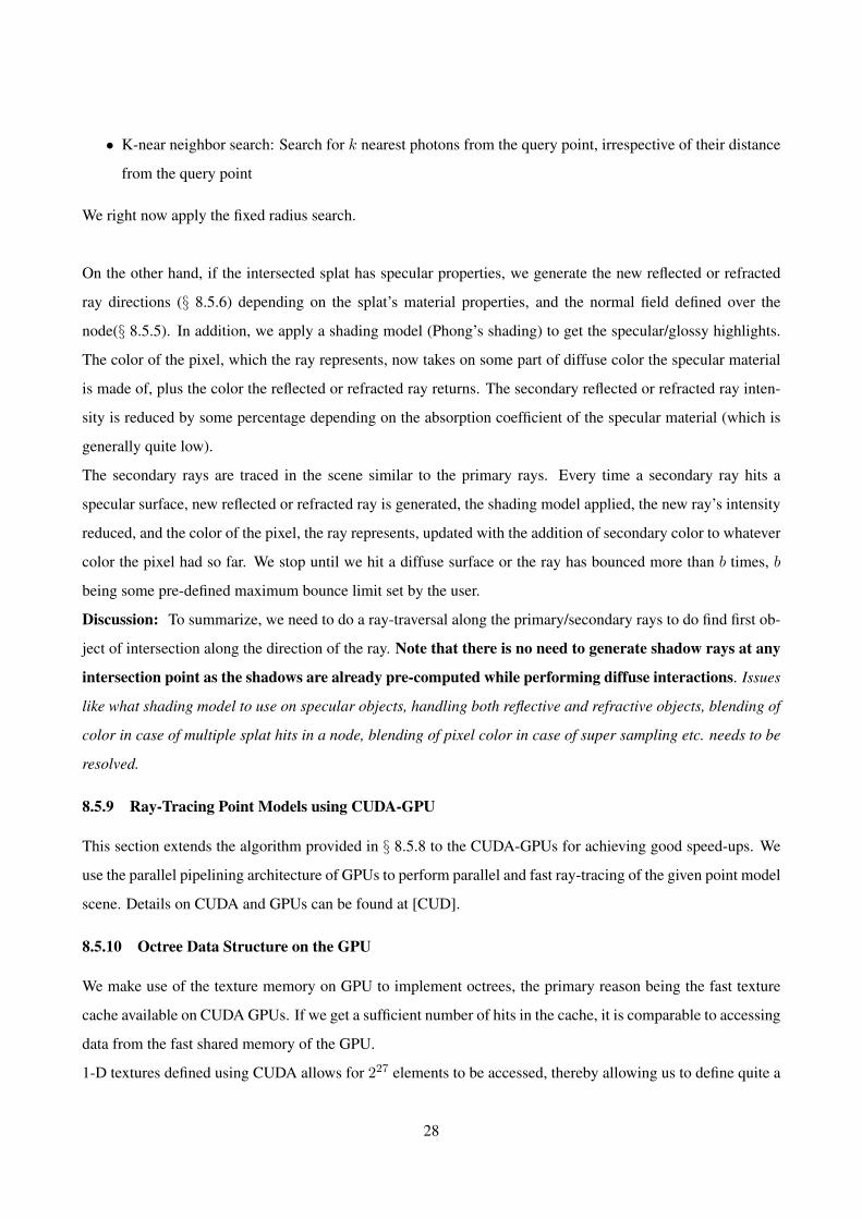
On the other hand, if the intersected splat has specular properties, we generate the new reflected or refracted
ray directions (§ 8.5.6) depending on the splat’s material properties, and the normal field defined over the
node(§ 8.5.5). In addition, we apply a shading model (Phong’s shading) to get the specular/glossy highlights.
The color of the pixel, which the ray represents, now takes on some part of diffuse color the specular material
is made of, plus the color the reflected or refracted ray returns. The secondary reflected or refracted ray inten-
sity is reduced by some percentage depending on the absorption coefficient of the specular material (which is
generally quite low).
The secondary rays are traced in the scene similar to the primary rays. Every time a secondary ray hits a
specular surface, new reflected or refracted ray is generated, the shading model applied, the new ray’s intensity
reduced, and the color of the pixel, the ray represents, updated with the addition of secondary color to whatever
color the pixel had so far. We stop until we hit a diffuse surface or the ray has bounced more than b times, b
being some pre-defined maximum bounce limit set by the user.
Discussion: To summarize, we need to do a ray-traversal along the primary/secondary rays to do find first ob-
ject of intersection along the direction of the ray. Note that there is no need to generate shadow rays at any
intersection point as the shadows are already pre-computed while performing diffuse interactions. Issues
like what shading model to use on specular objects, handling both reflective and refractive objects, blending of
color in case of multiple splat hits in a node, blending of pixel color in case of super sampling etc. needs to be
resolved.
8.5.9 Ray-Tracing Point Models using CUDA-GPU
This section extends the algorithm provided in § 8.5.8 to the CUDA-GPUs for achieving good speed-ups. We
use the parallel pipelining architecture of GPUs to perform parallel and fast ray-tracing of the given point model
scene. Details on CUDA and GPUs can be found at [CUD].
8.5.10 Octree Data Structure on the GPU
We make use of the texture memory on GPU to implement octrees, the primary reason being the fast texture
cache available on CUDA GPUs. If we get a sufficient number of hits in the cache, it is comparable to accessing
data from the fast shared memory of the GPU.
1-D textures defined using CUDA allows for 227 elements to be accessed, thereby allowing us to define quite a
28

deep octree. Each location in the texture is called a texel. A texel was primarily used for storing color values
(Red (R), Green (G), Blue (B), Alpha (A)). Each of these values can be 8−bits or 32−bits in size. Thus a texel
can store minimum of 32− bits of information to the maximum of 128− bits. We make use of these texels to
store the octree nodes and point data (instead of color values). Note that we want to minimize the storage per
node so that maximum number of nodes are present in the texture cache, and hence maximum cache hits are
possible.
To achieve a highly storage-efficient octree, we modify the octree to a N3 tree. With N = 2 this means that
every internal node has exactly 8 children. Thus even if a node has for example 6 filled children nodes and 2
empty nodes, we even store the 2 empty nodes in addition to the 6 filled nodes.
Pointer to I1 ‘s First Child
E E E E EL LL L L LLL L LLLLI1 I2
Pointer to I2 ‘s First Child
All 8 children of I1
grouped togetherAll 8 children of I2
grouped together
E – Empty Node
L – Leaf Node
I – Internal Node
Octree Node Pool in Texture memory
(a)
Node Texel – 32 bits
R G B A
8 bits 8 bits 8 bits 8 bits
30 bits used for storing address of the first child (if Internal Node) or address to the point data in data pool (if node is a leaf)
1 bit to check if the current node is empty
1 bit to check if the current node is a leaf
(b)
Figure 21: (a) Octree Node-Pool in texture memory of the GPU. All 8 children of any internal node are storedtogether in contiguous memory locations in the nodepool. (b) Every location in the nodepool is a 32 − bitstexel. It tells the address of the first child, whether the current node is a leaf or internal node and whether it isempty or not
As shown in Fig. 21 (a), all children of a node are grouped together. This saves memory, because a node
now needs just a single pointer to all its 8 children, thereby compromising the extra space taken up by empty
nodes. Each node (internal or leaf) is stored as a 32 − bit texel (Fig. 21 (b)). The first 30 − bits of the texel
holds the address of the first child of the internal node (the rest 7 children are stored contiguously in texture
29

memory after the first child) or the address to the data in case the node is a leaf. The remaining 2 bits are used
to identify whether the current node is empty or is it a leaf. We call this a node pool.
0 1
2 34
6
5
7
x=0 y=0 z=0
x=0 y=1 z=0
x=1 y=1 z=0
x=1 y=0 z=0
x=0 y=0 z=1
x=0 y=1 z=1
x=1 y=1 z=1
x=1 y=0 z=1
X
Z
Y
Figure 22: Figure shows 8 children of some internal node. All 8 children of any internal node are storedin contiguous memory locations in the nodepool. Further, these 8 children are stored in the SFC order i.e.according to their SFC index. In the figure, node 0 is stored before node 1, node 1 before node 2 and so on
Further, all the 8 children of any internal node are stored in some pre-defined order. We make use of a local
SFC ordering amongst the children (Fig 22). We store no other extra information in this memory-efficient
octree. Note that we do not require a parent pointer, as we always traverse downwards in the octree while
trying to figure the node containing some intersection point (§ 8.5.8). Further, the point data is also stored as
another 1D-texture. The details of the same are presented in § 8.5.12.
Thus, after having defined as to how the octree is stored in GPU’s texture memory, let us now take a closer look
at the math behind the octree traversal.
8.5.11 Fast Octree Traversal Algorithm
As seen in § 8.5.8, we need to trace along the ray. We find the ray’s intersection with the octree’s root, get the
intersection point (and increment by ∆), the leaf cell to which the intersection point belongs is determined, and
then algorithm continues from there.
30

As mentioned above, each traversal starts from the root node. During the traversal, the active node is interpreted
as a volume with range [0, 1]3. The ray’s origin p ∈ [0, 1]3 (3 is the dimension) is located within this node. Note
that p is a vector with (x, y, z) components, each normalized to the range [0, 1]. Now, it is necessary to find out
which child-node n is contains ray-origin p. Thus if R is the root node, we let p ∈ [0, 1]3 be the point’s local
co-ordinates in the root’s volume bounding box, and find child node n of root containing p. If c is the pointer
to the grouped children of the root node in the node pool, the offset to the child node n containing p is simply
int(p ∗N), the integer part of multiplication between p and N (N = 2) (since we have the N3 tree (§ 8.5.10)).
The formula is:
n = c + int(p ∗N)
Child node (0,0)
Child node (0,1)
Child node (1,1)
Child node (1,0)
c
p = (0.6,0.4)
n = c + int(p * N)= c + int((0.6*2, 0.4*2))= c + int((1.2,0.8))
= c + (1,0)
Pointer to I1 ‘s First Child
EI1
All 4 children of I1 grouped together in N2 Tree
E – Empty Node L – Leaf Node I – Internal Node
Octree Node Pool in Texture memory
c
EL L
c + (1,0) = c + (y*2 + x*1)= c + (1*2 + 0*1)= c + 2
= Third Child
jump of 2
Figure 23: Example node group in a node pool of a N2 tree with N = 2. This formula returns the valuec + (1, 0). c here is the pointer from the parent node to its first child in the nodepool. Value (1, 0) gives youthe child number (or the jump from the first child address) using the formula (y ∗2 + x∗1) i.e. (1∗2 + 0∗1)(in case of 3D it will be (z ∗ 4 + y ∗ 2 + x ∗ 1)). This formula works because we store the 8 children node ina specific SFC order
As explained in § 8.5.10, the child nodes are SFC ordered based on their location within the parent node.
Referring Fig. 23, we see the integer part of p ∗N gives us some x, y and z values. Given these values and the
SFC ordering we can figure out the child node which contains p.
Since the traversal is not finished yet, it is necessary to update the p to the range of the currently found child
node and continue the descent further. The appropriate formula to update p is:
p = p ∗N − int(p ∗N)
31

The new p is the remainder of the p ∗ N integer conversion. Now the traversal continues with the above
mentioned formulae, and loops until a leaf (or an empty node) is found. After finding the node containing the
point, the algorithm continues as mentioned in § 8.5.8. Note that this is just the SFC based traversal algorithm,
except we step through the SFC values, level by level, by calculating it on the fly (using the above formulae)
instead of pre-calculating it and then stepping through the needed bits. In addition to it, it is important to note
that even though a new descent is needed everytime a node is left, mostly the same pointers in the structure will
be followed, thus the hardware texture cache is very well prepared and appropriate.
8.5.12 Point Data Structure on the GPU
As mentioned in § 8.5.10, the input point data is also stored as an 1-D texture in the texture memory of the
GPU. Every point is the input data has the following attributes:
• Co-ordinates of the point (x, y, z – 3 floats)
• Normal at the point defining the local surface (n1, n2, n3 – 3 floats)
• Diffuse-Color of the point (c1, c2, c3 – 3 floats)
• Radius of the splat around the point (r – 1 float)
• Material Identifier, which stores the material properties, like reflectance, transmittance etc of the point
(mID – 1 float)
Each float occupies 4bytes (32−bits) in memory. Thus, with every point we need to store a total of 11 floats
or 44bytes. Note that each texel can hold a maximum of 128− bits of information (32− bits corresponding to
each of the R,G,B and A values in the texel). Thus, we can store maximum of 16bytes of data in a single texel.
As a result, we require 3 consecutive texels to store one single point data (3x16 = 48 bytes). We call this the
datapool.
Thus, in the case where we assume a single point per leaf, the data pointer in the leaf located in the node pool,
points to the corresponding point data in this data pool. To access all the information corresponding to the
particular point, we have to access 3 consecutive texels in the data pool memory.
However, a leaf seldomly contains just a single point. We divide the octree in the fashion such that each leaf
contains maximum of k points (roughly k is 10 to 25). Thus, to access all the k points belonging to the specific
leaf, we store all the k points in a contiguous fashion in 1D data pool texture memory. As number of points
varies from one leaf to another, we need to store the begin and end location of that contiguous block of points
for every leaf (beginP and endP ). As the leaf node is the part of octree node pool, it can store only one 32−bit
location, and hence can’t store both its beginP and endP locations.
32

LEAF L1
Octree Node Pool in Texture memory
beginP for Leaf L1
LEAF L2endP for Leaf L1 /beginP for
Leaf L2
beginP for Leaf L1
endP for Leaf L1 /beginP for
Leaf L2
Data Pool in Texture memory
All Points Belonging to LEAF L1
Begin-End Texture Pool
All Points Belonging to LEAF L2
endP for Leaf L2
Figure 24: A leaf in the nodepool points to some location in the Begin-End texture. This location gives us thestart of the contiguous block of points belonging to this leaf in the datapool (beginP). The next location in theBegin-End texture gives us the end of the block of points for this leaf (endP). This location also signifies thebeginP for some other leaf in the nodepool. Each texel location in the Begin-End texture is 32− bits in size
Thus, we now declare one more 1D texture (Fig. 24), viz a Begin-End texture, each texel representing one
32 − bits value. Each texel stores the beginP for some leaf and the texel next to it gives the endP for that
specific leaf. The leaf in the node pool now stores the texture pointer to the location containing its beginP .
Thus to access any point data after reaching the leaf, we follow the leaf pointer to this texture where we access
the beginP and endP location values. These values gives us the limits to the points, located in the data pool,
belonging to the current leaf. Further note that we need not explicitly store the endP locations for a leaf, as the
value in the next texel is the beginP for some other leaf and endP for the current one (this is valid because we
construct the octree in a specific fashion [Gor08]). Thus the size of the texture is equal to number of leaves in
the tree and not twice the number of leaves.
8.5.13 Multiple Leaves Per Splat
Many a times we face a situation where a point belongs to a particular leaf, but the splat that it represents
intersects more leaves than the one the point belongs to (Fig. 25 (a)). In such a scenario, ray tracing might go
for a toss and produce artifacts if these splats are not added to every leaf it intersects (Fig. 25 (b)) or they are
not considered if the ray intersects that leaf. As seen in Fig. 25 (b), even though the ray is intersecting splat
S, it gives a NULL intersection, as the point P representing S is located in the neighboring leaf and not the
current one.
33

cjrj
Sj
Icj
Sj
LEAF L1 LEAF L2
rj
(a) (b)
Figure 25: (a) A splat Sj’s center cj is located in one of the leaf nodes, but it intersects many leaves in the tree.In a situation, if some ray passes through one of the leaves Sj intersects, we have to check the ray’s intersectionwith Sj . Hence, splat Sj is inserted into all additional leaves it intersects (yellow cells) (b) It shows a situationwhere although a ray R intersects splat Sj , Sj is not considered since it belongs to some other leaf node. Thiswould eventually end p with the raytracer giving wrong output or an output with artifacts
Thus, these additional splat insertions are necessary as splats have an expansion and may stretch over several
leaves. Hence, further splat insertions are made in the leaves, however we keep the structure of the octree the
same i.e. no additional sub-divisions are made.
Sj
E
Sj
E
(a) (b)
Figure 26: We check whether the edges of the bounding square of splat Sj intersect the planes E that boundthe octree leaf cell. (a) Sj is inserted into the cell. (b) Sj is not inserted into the cell. This test is only performedif the first test (bounding box test) is positive
34

LEAF L1
Octree Node Pool in Texture memory
beginP for Leaf L1
LEAF L2endP for Leaf L1 /beginP for
Leaf L2
beginP for Leaf L1
endP for Leaf L1 /beginP for
Leaf L2
Data Pool in Texture memory
All Points Belonging to LEAF L1
Begin-End Texture Pool
All Points Belonging to LEAF L2
endP for Leaf L2
E E1 E2 E3 E4
E3 E1 E4 E2
Figure 27: A leaf in the nodepool points to some location in the beginEnd texture. This location gives usthe start of the contiguous block of points belonging to this leaf in the datapool (beginP). The next location,now, gives the number of extra splats (say E extra splats) added to this leaf (in the case shown above E = 4).The next E locations stores the addresses of these added splats. The location after this, gives the endP of thecurrent leaf or in other words, the beginP of the new leaf
Since performing such an exact cell-splat intersection is computationally rather expensive, we insert the
splats into leaf cells that potentially intersect the splat. For each splat Sj we traverse the tree top-down applying
a nested test for each traversed cell. The first test checks for splat Sj whether the axes-aligned box with center
cj and side length 2 · rj intersects the cell. If the test fails, tree traversal for that branch stops. For all leaf cells,
for which the first test was positive, we perform a second test. The second test uses the local parameterization
of the splat. The local parameters (0, 0), (0, 1), (1, 0), and (1, 1) define a 2D square that bounds the splat. We
check the position of these four points against the leaf cell. If all four points lie on one side of one of the six
planes that bound the leaf cell, the splat cannot intersect the leaf cell, see Fig. 25 (b). Otherwise, we insert the
splat into the leaf cell, see Fig. 26 (a).
This nested test is very simple and fast, yet produces no false negatives and only few false positives. False
positives means that we store a splat more often than necessary, which may impact the performance of the ray
tracing. False negatives, on the other hand, would mean that we miss some splats, which would actually impact
the correctness.
Adding splats to every intersecting leaf is easy, but it actually means adding 44 bytes of data per splat to every
leaf it intersects. This drastically can increase the memory requirements for the data pool texture memory. To
avoid this situation we store only the address of the intersecting splat (4 bytes) for a particular leaf instead of
35

replicating the entire splat. Thus now, if a ray intersects a leaf, all the splats originally inside that leaf as well
as the splats from surrounding areas intersecting that leaf are checked for intersection with the ray.
We need to make some amendments in the Begin-End texture (as in § 8.5.12) so as to accommodate the ad-
dresses of these new splats. Referring Fig. 27, we see a leaf points to some corresponding location in the
Begin-End texture. This texel location stores the beginP for that leaf. beginP gives the beginning location
of the contiguous block of points belonging to that leaf in the data pool texture. The next texel location in the
Begin-End texture gives the number of extra splats (say E extra splats) added to this leaf. The next E locations
store the addresses of these added splats. The location after this, gives the endP of the current leaf or in other
words, the beginP of the new leaf. Thus, we add the addresses of those extra splats between the beginP and
endP of the current leaf in the Begin-End texture memory.
8.5.14 Coherent Rays and Super-Sampling
Sending out only a single ray per pixel might get us into aliasing troubles. Thus, it is appropriate to either
render larger images and downscale them for achieving anti-aliasing, or send multiple random rays per pixel
and do super-sampling. The final color of the pixel is some weighted average of the colors returned by the rays
shot from that pixel.
View Plane
Eye/Camera
View Plane
Eye/Camera
R1 R1
R4
R2R3
R4
R3R2
Y Axis Y Axis
(a) (b)
Figure 28: As we can see (figure on left), rays take up more divergent paths if sent out in a linear fashionas per pixel placements. If the rays are sent out w.r.t 2 × 2 pixel blocks, the coherence of these ray paths iscomparatively very high (figure on right)
36

It however does mean that we are sending more number of rays for rendering a frame of the scene, thereby
increasing the running time linearly with the number of ray samples. However, this theory holds good if we
are performing ray-tracing on the CPU. While on GPU, larger number of rays per pixel will gather smaller
and smaller overhead, the reason being their coherence. Since all these rays travel the same path (mostly),
the amount of warp divergence will be very low. Further, referring Fig. 28, instead of sending rays in a linear
fashion as per the pixel placements, if we send them in a 2D block fashion, say rays from 2 × 2 pixel block,
the coherence of these ray paths is comparatively very high. Thus in a 2 × 2 pixel scenario, if we do 8×
super-sampling (8 rays per pixel), the entire warp (8× 4 threads) will be well behaved, mostly. Since, they will
mostly travel the same paths, the texture cache hits will also be high resulting in fast data access and execution.
Discussion: The data is arranged in 3 different textures stored on the GPU, one a node-pool, another a data-pool
and the third one (Begin-End texture) acting as a bridge between the node and data pool textures. Ray-Tracing
is performed as per the algorithm mentioned in § 8.5.8. Coherent, super-sampled rays are sent out and parallel
execution of finding intersections of those rays with the first-hit objects is performed on the GPU. The secondary
rays are appropriately generated and are traced till they hit the background or some diffuse surface. Fast, ray-
tracing algorithm combines advantages of the algorithm used to quickly find the leaf containing some point
while traversing along the ray and the usage of texture cache to get maximum hits for a set of coherent rays.
Appropriate reflection, refraction models are applied to compute the color values of every pixel in the scene.
8.5.15 Fusing Diffuse Global Illumination and Ray Tracing Together
Given a scene comprising of point based models, it is a mixed bag of both specular and diffuse objects. One
important issue is handling the fact that FMM based diffuse global illumination only covers the LDD∗ and
ignores any contribution from specular splats (LS+D), nor does it transfer any energy to them (LD∗S+), as
the paths LS+D and LDS∗ are handled during ray-tracing. Thus, while performing FMM on the given point
model scene [Gor07], we simply ignore the contributions of specular leaves during the pull phase and simply
ignore transfer of energy to specular leaves during the last stage of push phase of the FMM. As far as the V-Map
for the scene is concerned, no changes are made as the visible links between any diffuse and specular nodes or
between two specular nodes are simply ignored. The transfer of energy due to these links is accounted for in
ray-tracing. Thus, this completes the whole set-up of a complete global illumination package for point models.
37
9 Results
As we have seen, all the algorithms have been worked out. However, the implementation is in progress and it
would take some while to get the results. I am hoping some results come up by the time of the APS presentation,
else the results will be mailed within some days after the presentation.
10 Conclusion and Report Summary
Point-sampled geometry has gained significant interest due to their simplicity. The lack of connectivity touted
as a plus, however, creates difficulties in many operations like generating global illumination effects. This
becomes especially true when we have a complex scene consisting of several models, the data for which is
available as hard to segment aggregated point-based models. Inter-reflections in such complex scenes requires
knowledge of visibility between point pairs. Computing visibility for point models becomes all the more diffi-
cult, than for polygonal models, since we do not have any surface or object information.
Point-to-Point Visibility is arguably one of the most difficult problems in rendering since the interaction be-
tween two primitives depends on the rest of the scene. One way to reduce the difficulty is to consider clustering
of regions such that their mutual visibility is resolved at a group level. Most scenes admit clustering, and the
Visibility Map data structure we propose enables efficient answer to common rendering queries.
V-Map was used in a diffuse global illumination solution using FMM on point models. Both the V-Map as well
as the FMM algorithm were implemented in parallel on the GPU which reported efficient speed-ups. V-Map
was used here to solve point-to-point view independent visibility queries between octree nodes.
We then extended V-Map to trace caustic photons through the point model scene and capture them on the target
diffuse surfaces. The visible list (part of the V-Map) of the light source (and its ancestors) assisted in sending
rays only to visible specular leaf nodes. This accounts for a lot of time-saving, as we don’t have to send packets
of rays in every direction from the light source searching for the probable caustic generators. Normal fields
were generated for each specular leaf so as to enable accurate secondary ray directions. The factors like num-
ber of photons to be send, and where to send were in sync with the emissive power of the light source and the
area occupied by the splat as seen from the light source (using the subtended solid angle). Kd-tree was used to
organize the caustic photon map, thereby enabling fast caustic photon retrieval during ray-tracing.
We used an efficient, but naive, octree traversal algorithm (on GPU) to do photon tracing as well as ray-trace
rendering. The texture cache on GPU was used for efficient octree storage and fast traversal through it, to get
answers to first-object intersection queries for ray-tracing. Point data was also organized into a 1D texture on
GPU memory, directly accessible by leaves of the octree. Provision for multiple leaves per splat was added to
avoid undesirable holes and artifacts during ray-trace rendering. Coherent rays and super-sampling was per-
38

formed to aid a well behaved warp on GPU and avoid aliasing artifacts.
As the diffuse global illumination solution is view-independent, it provides us with an advantage of having an
interactive walk-through of the input scene of point models. However, specular effects being view-dependent
needs to be calculated for every new view-point in the ray-trace rendered frame. Thus, if specular effect gen-
eration takes a lot of time, we loose out of having an interactive walk-through of the scene. We desire not to
loose this advantage, and try to give a fast time-efficient algorithm for specular effects generation.
Global Illumination of Point Models
Diffuse Effects Specular Effects
V-Map FMM
GPU
Caustics Reflections Refractions
Fast Octree Traversal for Ray-TracingRay-Splat IntersectionsNormal Field on Splats
Coherent RaysSuper-Sampling
Text
ure
Cac
he
m
em
ory
Photon GenerationKd-Trees
Figure 29: Work-flow of my thesis. Capturing Global Illumination Effects on Point Models.
Issues pertaining to shading to be applied to specular glossy objects, blending of color in case a ray hits
multiple splats in an octree-leaf, blending of color for a single pixel in case of super-sampling, handling semi-
transparent and reflective plus refractive objects, setting up various material properties etc. needs to be handled.
We can say the base system is ready, only some tweaks and make-ups remain to make the output image beautiful
and visually pleasing.
39

The diffuse global illumination and ray-tracing systems have been correctly merged so as to give a complete
global illumination package for point models. We, thus, have a two–pass global illumination solver for point
models. The input to the system is a scene consisting of both diffuse and specular point models. First pass
calculates the diffuse illumination maps, followed by the second pass for specular effects. Finally, the scene is
rendered using our ray-tracing technique. As my last note, I would like to provide, for your reference, a simple
work-flow of the work done by me during the entire period of my Ph.d and how each module gels with the
other to give a complete story to my thesis. Fig. 29 gives a pictorial view of the work-flow of my thesis.
References
[AA03] Anders Adamson and Marc Alexa. Ray tracing point set surfaces. In SMI ’03: Proceedings of
the Shape Modeling International 2003, page 272, Washington, DC, USA, 2003. IEEE Computer
Society. 14
[AGCA08] Prekshu Ajmera, Rhushabh Goradia, Sharat Chandran, and Srinivas Aluru. Fast, parallel, gpu-
based construction of space filling curves and octrees. In SI3D ’08: Proceedings of the 2008
symposium on Interactive 3D graphics and games, pages 1–1, New York, NY, USA, 2008. ACM.
3
[CUD] CUDA. NVIDIA CUDA Programming Guide. http://developer.nvidia.com/cuda.
2, 9, 28
[DBMS02] K. Dmitriev, S. Brabec, K. Myszkowski, and H. Seidel. Interactive global illumination using
selective photon tracing. In 13th Eurographics Workshop on Rendering, pages 21–34, 2002. 18
[GAC08] R. Goradia, P. Ajmera, and S. Chandran. Gpu-based hierarchical computation for view indepen-
dent visibility. Accepted at ICVGIP, Indian Conference on Vision, Graphics and Image Processing,
2008. 2, 3, 10
[GD07] Nail A. Gumerov and Ramani Duraiswami. Fast multipole methods on graphics processors. Astro
GPU, 2007.
[GKCD07] R. Goradia, A. Kanakanti, S. Chandran, and A. Datta. Visibility map for global illumination
in point clouds. Proceedings of ACM SIGGRAPH GRAPHITE, 5th International Conference on
Computer Graphics and Interactive Techniques, 2007. 2, 3, 8, 9
[Gor06] Rhushabh Goradia. Fmm-based illumination maps for point models. Second Progress Report,
Ph.D., 2006. 2
40

[Gor07] Rhushabh Goradia. Global illumination for point models. Third Progress Report, Ph.D., 2007. 2,
9, 18, 37
[Gor08] Rhushabh Goradia. Fast, gpu-based diffuse global illumination for point models. Fourth Progress
Report, Ph.D., 2008. 2, 9, 10, 33
[GWS04] Johannes Gunther, Ingo Wald, and Philipp Slusallek. Realtime caustics using distributed photon
mapping. In Rendering Techniques, pages 111–121, jun 2004. (Proceedings of the 15th Euro-
graphics Symposium on Rendering). 18
[Hec90] P. S. Heckbert. Adaptive radiosity textures for bidirectional ray tracing. Computer Graphics, ACM
Siggraph Conference proceedings, pages 145–154, 1990.
[Jen96] H. W. Jensen. Global illumination using photon maps. Eurographics Rendering Workshop 1996,
pages 21–30, June 1996. 14
[KC03] A. Karapurkar and S. Chandran. Fmm-based global illumination for polygonal models. Master’s
thesis, Indian Institute of Technology, Bombay, 2003. 5
[KGC04] A. Karapurkar, N. Goel, and S. Chandran. Fmm-based global illumination for polygonal models.
Indian Conference on Computer Vision, Graphics, and Image Processing, pages 119–125, 2004.
[LMR07] Lars Linsen, Karsten Muller, and Paul Rosenthal. Splat-based ray tracing of point clouds. Journal
of WSCG, 2007. 14, 22
[MA] David M. Mount and Sunil Arya. Ann: A library for approximate nearest neighbor searching.
http://www.cs.umd.edu/˜mount/ANN/. (Last seen on 21st August, 2009). 25
[PZvBG00] Hanspeter Pfister, Matthias Zwicker, Jeroen van Baar, and Markus Gross. Surfels: Surface ele-
ments as rendering primitives. In Kurt Akeley, editor, Siggraph 2000, Computer Graphics Pro-
ceedings, pages 335–342. ACM Press / ACM SIGGRAPH / Addison Wesley Longman, 2000.
4
[RL00] Szymon Rusinkiewicz and Marc Levoy. QSplat: A multiresolution point rendering system for
large meshes. In Kurt Akeley, editor, Siggraph 2000, Computer Graphics Proceedings, pages
343–352. ACM Press / ACM SIGGRAPH / Addison Wesley Longman, 2000. 4
[SJ00] G. Schaufler and H. Jensen. Ray tracing point sampled geometry. In Eurographics Rendering
Workshop Proceedings, pages 319–328, 2000. 14
41

[Wal05] Ingo Wald. High-Quality Global Illumination Walkthroughs using Discretized Incident Radiance
Maps. Technical Report, SCI Institute, University of Utah, No UUSCI-2005-010 (submitted for
publication), 2005.
[Wika] Wikipedia. K-means clustering algorithm. http://en.wikipedia.org/wiki/
K-means_clustering. (Last seen on 20th August, 2009).
[Wikb] Wikipedia. Kd-tree. http://en.wikipedia.org/wiki/Kd-tree. (Last seen on 21st
August, 2009). 25
[WS03] Michael Wand and Wolfgang Straer. Multi-resolution point-sample raytracing. Graphics Inter-
face, pages 139–148, 2003. 4, 14
[WS05] Ingo Wald and Hans-Peter Seidel. Interactive Ray Tracing of Point Based Models. In Proceedings
of 2005 Symposium on Point Based Graphics, 2005. 14
42