global financial markets remain dependent on central banks

25BIS 85th Annual Report

II. Global financial markets remain dependent on central banks

During the period under review, from mid-2014 to end-May 2015, accommodative monetary policies continued to lift prices in global asset markets. Investors’ risk-taking remained strong as expectations of policy rate increases were pushed out further and additional asset purchases undertaken. As a result, bond prices climbed, equity indices repeatedly hit new highs and prices of other risky assets also rose. Moreover, global investors’ exposure to riskier assets continued to increase.

As central banks remained in easing mode, bond yields in advanced economies continued to fall throughout much of the period under review. In a number of cases, bond markets entered uncharted territory as nominal bond yields fell below zero for maturities even beyond five years. This was mainly due to falling term premia, but also reflected downward revisions of expected future policy rates. Towards the end of the period, bond markets – in particular in Europe – saw sharp yield reversals as investors became increasingly uneasy about stretched valuations.

Signs of market fragility were evident more widely too. Bouts of volatility occurred with increasing frequency across markets, and signs of illiquidity in fixed income markets began to appear. As market-makers have scaled back their activities after the Great Financial Crisis, asset managers have become more important as sources of liquidity. Such shifts, in combination with increased official demand, may have reduced liquidity and reinforced liquidity illusion in certain bond markets.

Expectations of increasingly divergent monetary policies in the United States and the euro area resulted in widening interest rate differentials, and, as a result, the dollar soared and the euro plummeted. In addition to these outsize exchange rate swings, foreign exchange markets saw big rate moves more generally. These included the surge of the Swiss franc following the Swiss National Bank’s discontinuation of its minimum exchange rate against the euro, and rapid depreciation of currencies for a number of energy-producing countries.

In parallel with the dollar’s surge, oil prices fell sharply in the second half of 2014 before stabilising and recovering somewhat in the second quarter of 2015. Although the oil price drop was particularly severe, commodity prices declined more generally. The rapid price moves in commodity markets reflected a combination of weak demand, in particular from EMEs, and, in the case of oil, stronger supply. But they may also have reflected increased activity on the part of financial investors in commodity markets, as these markets are becoming a more integral part of global financial markets more broadly, as well as rising indebtedness in the energy sector.

The first section of this chapter describes the main developments in global financial markets between mid-2014 and end-May 2015. The second focuses on the extraordinarily low yields in government bond markets. The third section explores rising fragilities in financial markets, with emphasis on risks of liquidity illusion in fixed income markets. The final section discusses the growing linkages between commodities – in particular oil – and financial markets.

26 BIS 85th Annual Report

Further monetary accommodation but diverging outlook

Increasing macroeconomic and monetary policy divergence during the past year set the scene for global financial markets. The United States, in particular, continued to recover while the euro area, Japan and a number of emerging market economies (EMEs) faced weakening growth prospects during much of the period under review (Chapter III). Against this backdrop, actual and expected monetary policy moves diverged. The US Federal Reserve ended its large-scale asset purchase programme and continued to take gradual steps to prepare markets for an eventual increase in the federal funds target rate. Still, as global disinflationary pressures grew, largely due to falling oil prices, the vast majority of central banks eased policy (Chapter IV). As a result, US forward interest rates diverged from forward rates elsewhere, especially vis-à-vis the euro area (Graph II.1, left-hand panel).

The renewed wave of monetary accommodation supported prices across asset classes. As near zero interest rate expectations were pushed out further and additional asset purchases undertaken, yields on government bonds fell to record lows in a number of advanced economies (Graph II.1, centre panel). Moreover, a growing share of sovereign debt traded at negative yield levels (see discussion below). The fall in euro area bond yields that had begun in 2014 accelerated in early 2015 as the ECB launched its expanded asset purchase programme. As a result, 10-year government bond yields in Germany fell to levels as low as 7.5 basis points in April 2015. Those for a number of other euro area countries, including France, Italy and Spain, also reached record lows. Even in Japan, where bond yields have been exceptionally low for many years, 10-year bond yields reached a new trough of 20 basis points in January 2015. However, a sharp global yield reversal in late April and May 2015 suggested that investors had viewed some of the previous declines as excessive.

Much of the decline in yields that took place up to April 2015 reflected falling term premia (see below). Expectations that near zero policy interest rates would

Easier monetary policies support asset prices Graph II.1

Forward interest rate curves1 Long-term government bond yields Stock prices Per cent Per cent Per cent 4 Jan 2013 = 100

1 For the United States, 30-day federal funds rate futures; for the euro area, three-month Euribor futures. 2 JPMorgan GBI-EM Broad Diversified Index, yield to maturity in local currency. 3 Ten-year government bond yields. 4 MSCI Emerging Markets Index.

Sources: Bloomberg; Datastream.

0.0

0.4

0.8

1.2

1.6

2.0

2014 2015 2016 2017

2 June 2014 31 Dec 2014 29 May 2015

United States: Euro area:

0.0

1.1

2.2

3.3

4.4

5.5

6.6

0.0

0.5

1.0

1.5

2.0

2.5

3.0

2013 2014 2015

EMEs2Lhs:

United StatesGermanyUnitedKingdomJapan

Rhs:3

80

100

120

140

160

180

200

2013 2014 2015S&P 500EURO STOXXShanghai Composite

Nikkei 225EMEs4


remain in place for longer than previously anticipated also played a role, especially at shorter maturities. Central bank purchases of government bonds added to the downward pressure on premia and yields, as did the move by some central banks to negative policy rates. Expectations that the Federal Reserve was inching closer to its first rate hike kept the level of US bond yields somewhat higher than in several other advanced economies. But US yields nevertheless continued to fall at a moderate pace throughout the second half of 2014 and into early 2015 before the decline was halted (Graph II.1, centre panel).

In parallel with the drop in bond yields, investors continued to exhibit a strong search for yield. As a result, equity prices rose to record highs in many markets (Graph II.1, right-hand panel), even as the macroeconomic outlook remained relatively weak (Annex Table A1). Although EME equity markets were generally less buoyant, there were exceptions: the Shanghai Composite index surged by 125% during the period under review, despite mounting reports of a slowing Chinese economy. As valuations became increasingly stretched, equity prices underwent a few sharp but brief corrections in late April and May 2015.

Signs of stronger risk-taking were evident in market prices as well as in quantity-based indicators. Global P/E ratios continued on an upward trek that had started in 2012, which brought them above the median value both for the past decade and since 1987 (Graph II.2, left-hand panel). In the syndicated loan market, the share of leveraged loans, which are granted to low-rated and highly leveraged borrowers, rose to almost 40% of new signings in April and May 2015 (Graph II.2, centre panel). And the share of those loans featuring creditor protection in the form of covenants stayed very low (Graph II.2, right-hand panel).

Global investors’ increased exposure to riskier asset classes was also evident in EME corporate bond markets. Corporations in EMEs have issued growing amounts of debt in international markets at progressively longer maturities since 2010 (Graph II.3, left-hand panel). At the same time, the debt servicing capacity of EME

Signs of increased financial risk-taking Graph II.2

World price/earnings ratio Syndicated lending, global signings2 Covenants, leveraged facilities2 USD bn Per cent Per cent Per cent

1 Twelve-month forward price/earnings ratio of the world equity index compiled by Datastream. 2 Based on data available up to 21 May 2015; “leveraged” includes “highly leveraged”. 3 Of leveraged loans in total syndicated loan signings.

Sources: Datastream; Dealogic; BIS calculations.

8

10

12

14

16

05 06 07 08 09 10 11 12 13 14 15Forward P/E ratio1

Median value since 1987Median value since 2005

0

175

350

525

700

8

16

24

32

40

05 06 07 08 09 10 11 12 13 14 15

Not leveragedLeveraged

Lhs:Share3

Rhs:

0

1

2

3

0

7

14

21

05 06 07 08 09 10 11 12 13 14 15

With covenant(s) with respect tocurrent ratio or net worth (lhs)With at least one identifiedcovenant (rhs)

Value share of new issuance:


corporate bond issuers has deteriorated. In particular, the leverage ratio of EME corporations has been increasing fast to reach the highest level in a decade, exceeding that of advanced economy corporations, both for entities issuing internationally and for those financing themselves in domestic debt markets (Graph II.3, centre panel). Despite the strong issuance and increased riskiness of EME corporate bonds, investors have generally not pushed up their required risk premium (Graph II.3, right-hand panel).

Outsize exchange rate moves during the past year were a key manifestation of the substantial influence of monetary policy on financial markets. The US dollar experienced one of the largest and fastest appreciations on record, surging by around 15% in trade-weighted terms between mid-2014 and the first quarter of 2015 before stabilising (Graph II.4, left-hand panel). At the same time, the euro dropped by more than 10%. Reflecting divergent monetary policy stances, the widening interest rate differential between dollar and euro debt securities increasingly encouraged investors to move into dollar assets, seemingly playing a bigger role than in the past (Graph II.4, centre panel). This underscores the growing importance of policy rate expectations for exchange rate developments.

As exchange rates became increasingly sensitive to monetary policy expectations, equity prices became more responsive to exchange rate movements. This was particularly so in the euro area, where since 2014 a statistically significant relationship has emerged between returns on the EURO STOXX index and the euro/US dollar exchange rate. Specifically, a 1% depreciation of the euro has, on average, coincided with a rise in equity prices of around 0.8% (Graph II.4, right-hand panel). No such relationship had been apparent previously, from the introduction of the euro.

Increasing duration and credit risk for EME corporate bond investors Graph II.3

Gross issuance and maturity of EME international corporate bonds1

Leverage ratio of corporations in EMEs and advanced economies2

US dollar-denominated EME corporate bond index3

Average maturity in years Ratio, annualised Basis points

1 Sum of issuance by non-financial and non-bank financial corporations of EMEs by residence. The size of balloons reflects relative volumeof gross issuance in each year. The figure next to the balloon for 2014 is the amount of gross issuance in 2014 in billions of US dollars. EMEs: Brazil, Bulgaria, Chile, China, Colombia, the Czech Republic, Estonia, Hong Kong SAR, Hungary, Iceland, India, Indonesia, Korea, Latvia, Lithuania, Malaysia, Mexico, Peru, the Philippines, Poland, Romania, Russia, Singapore, Slovenia, South Africa, Thailand, Turkey and Venezuela. 2 Leverage ratio = total debt/EBITDA, where EBITDA is earnings before interest, tax, depreciation and amortisation; calculatedas a trailing four-quarter moving average; EMEs are those listed in footnote 1; advanced economies are the euro area, Japan, the United Kingdom and the United States. 3 JPMorgan CEMBI Broad Diversified index. 4 Spread over US Treasuries.

Sources: JPMorgan Chase; S&P Capital IQ; BIS international debt securities database; BIS calculations.

6

8

10

12

14

04 05 06 07 08 09 10 11 12 13 14 15

138

Yearly data Data up to March 2015

1.0

1.5

2.0

2.5

3.0

05 06 07 08 09 10 11 12 13 14

All bond issuers International bond issuers

EMEs: Advancedeconomies:

0

300

600

900

1,200

04 05 06 07 08 09 10 11 12 13 14 15Strip spread4 Yield to maturity


Just like foreign exchange markets, commodity markets saw broad-based price swings, with oil prices falling particularly sharply. The price of West Texas Intermediate (WTI) crude oil fell from above $105 in mid-2014 to $45 per barrel in January 2015 before stabilising and partially recovering (Graph II.5, left-hand panel).

The dollar soars, the euro plunges Graph II.4

Diverging dollar and euro EUR/USD vs yield differential2 Equity sensitivity to euro exchange rate2, 4

1 Jan 2013 = 100

1 BIS nominal effective exchange rate broad indices. A decline (increase) indicates a depreciation (appreciation) of the currency in trade-weighted terms. 2 End-of-week observations. 3 Two-year government bond yield differential between the United States and Germany(in percentage points). 4 A positive (negative) EUR/USD log difference corresponds to an appreciation (depreciation) of the euro vis-à-vis the dollar.

Sources: Bloomberg; BIS; BIS calculations.

Oil plunge puts energy sector under pressure Graph II.5

Commodity prices drop Energy sector underperforms Corporate credit spreads4 2 Jun 2014 = 100 Basis points 2 Jun 2014 = 100 Basis points Basis points

1 Commodity Research Bureau – Bureau of Labor Statistics. 2 The difference between the option-adjusted spreads of investment grade debt of energy sector corporates and the overall corporate sector for EMEs, the euro area and the United States (computed as a simple average). The EME energy sector index consists of both investment grade and high-yield debt. 3 Simple average of energy stock prices; for the United States, S&P 500 equity index; for the euro area and EMEs, the MSCI. 4 Option-adjusted spreads over US Treasury notes.

Sources: Bank of America Merrill Lynch; Bloomberg; Datastream.

90

100

110

120

2013 2014 2015

US dollarEuro

Effective exchange rates:1

0.96

1.12

1.28

1.44

–1.0 –0.5 0.0 0.5 1.0 1.5

EUR/

USD

Two-year government bond differential3

2009–13 2014 onwards

–0.2

–0.1

0.0

0.1

–0.06 –0.03 0.00 0.03 0.06

EURO

STO

XX re

turn

EUR/USD log difference

1999–2013 2014 onwards

25

40

55

70

85

100

Q3 14 Q4 14 Q1 15 Q2 15Oil (WTI)Copper All commodities

Foodstuffs

CRB BLS1 Indices:

30

60

90

120

150

180

62.5

70.0

77.5

85.0

92.5

100.0

Q3 14 Q4 14 Q1 15 Q2 15

Corporate spread (lhs)2

Stock index (rhs)3

Energy sector:

50

100

150

200

250

300

150

350

550

750

950

1,150

Q3 14 Q4 14 Q1 15 Q2 15

United States Euro area EMEs

Investmentgrade (lhs):

High-yield(rhs):

The dollar soars, the euro plunges Graph II.4

Diverging dollar and euro EUR/USD vs yield differential2 Equity sensitivity to euro exchange rate2, 4

1 Jan 2013 = 100

1 BIS nominal effective exchange rate broad indices. A decline (increase) indicates a depreciation (appreciation) of the currency in trade-weighted terms. 2 End-of-week observations. 3 Two-year government bond yield differential between the United States and Germany(in percentage points). 4 A positive (negative) EUR/USD log difference corresponds to an appreciation (depreciation) of the euro vis-à-vis the dollar.

Sources: Bloomberg; BIS; BIS calculations.

Oil plunge puts energy sector under pressure Graph II.5

Commodity prices drop Energy sector underperforms Corporate credit spreads4 2 Jun 2014 = 100 Basis points 2 Jun 2014 = 100 Basis points Basis points

1 Commodity Research Bureau – Bureau of Labor Statistics. 2 The difference between the option-adjusted spreads of investment grade debt of energy sector corporates and the overall corporate sector for EMEs, the euro area and the United States (computed as a simple average). The EME energy sector index consists of both investment grade and high-yield debt. 3 Simple average of energy stock prices; for the United States, S&P 500 equity index; for the euro area and EMEs, the MSCI. 4 Option-adjusted spreads over US Treasury notes.

Sources: Bank of America Merrill Lynch; Bloomberg; Datastream.

90

100

110

120

2013 2014 2015

US dollarEuro

Effective exchange rates:1

0.96

1.12

1.28

1.44

–1.0 –0.5 0.0 0.5 1.0 1.5EU

R/US

DTwo-year government bond differential3

2009–13 2014 onwards

–0.2

–0.1

0.0

0.1

–0.06 –0.03 0.00 0.03 0.06

EURO

STO

XX re

turn

EUR/USD log difference

1999–2013 2014 onwards

25

40

55

70

85

100

Q3 14 Q4 14 Q1 15 Q2 15Oil (WTI)Copper All commodities

Foodstuffs

CRB BLS1 Indices:

30

60

90

120

150

180

62.5

70.0

77.5

85.0

92.5

100.0

Q3 14 Q4 14 Q1 15 Q2 15

Corporate spread (lhs)2

Stock index (rhs)3

Energy sector:

50

100

150

200

250

300

150

350

550

750

950

1,150

Q3 14 Q4 14 Q1 15 Q2 15

United States Euro area EMEs

Investmentgrade (lhs):

High-yield(rhs):


Box II.AThe oil price: financial or physical?

Oil and, more generally, energy are key production inputs. The oil price, therefore, is an important determinant of production decisions and also has a significant impact on inflation dynamics. This box discusses the interaction of physical and financial prices, with a specific focus on two aspects. The first is the extent to which oil is akin to conventional financial assets: price swings are driven by changes in expectations, not only by the current conditions in the physical market. The second is the relationship of the oil futures curve with the physical market: as the shape of the former is determined by current conditions of the physical market, it would be misleading to interpret it as an indicator of the expected price path.

Over the past decade, as financial activity in oil and other markets surged, many commentators started referring to commodities as an asset class. The analogy is warranted to some extent: popular oil price benchmarks such as Brent and West Texas Intermediate (WTI) are actually futures, and their price depends on players’ interaction in the futures markets. However, oil is a physical asset, and the futures contracts are backed by it. So, futures and physical prices must be tied together: should a misalignment between conditions in the physical market and in the futures market materialise, players can store oil and sell it forward (or vice versa), eventually bringing prices back into line. Consequently, while physical prices are normally less volatile, they track quite closely the futures benchmarks (Graph II.A, left-hand panel).

The parallel between conventional assets and oil extends also to the futures curve. For a conventional asset, the difference between spot and futures prices (the so-called basis) is determined by the cost of carry (largely a function of interest rates), and by the stream of dividends and interest payments that the asset yields. Oil generates no cash stream, but agents attach a premium to holding it physically because of its value for production and consumption rather than on paper – the so-called convenience yield. The convenience yield is unobservable, and varies over time according to the conditions of the underlying physical market: at times of tightness, the convenience yield would be high, as agents attach a high value to holding a scarce resource. By contrast, the convenience yield could even turn negative when supply is abundant in the physical market and inventories are high: in such a situation, holding physical oil is not advantageous, as slack in the physical market would ensure easy access to the resource in case of need. So, while the oil futures curve is normally negatively sloped (backwardation) due to a positive convenience yield, its slope can turn positive (contango) at times of inventory overhang. It is therefore no surprise that the futures curve currently slopes upwards (Graph II.A, right-hand panel).

An important consequence of the presence of a convenience yield is that it would be wrong to interpret a positively (or negatively) sloped supply curve as evidence of bullish (or bearish) expectations. The price of any

Rising energy sector debt and widening spreads Graph II.14

US corporate bonds outstanding1 EME corporate bonds outstanding2 High-yield US corporate bond spreads3

USD bn USD trn USD bn USD trn Basis points

1 Face value of Merrill Lynch high-yield and investment grade corporate bond indices. 2 Face value; energy sector includes oil & gas and utility & energy firms; bonds issued in US dollars and other foreign currency by firms based in Brazil, Bulgaria, Chile, China, Colombia, the Czech Republic, Estonia, Hong Kong SAR, Hungary, India, Indonesia, Israel, Korea, Latvia, Lithuania, Mexico, Peru, the Philippines, Poland, Romania, Russia, Singapore, Slovenia, South Africa, Thailand, Turkey and Venezuela. 3 Option-adjusted spread over US Treasury notes.

Sources: Bank of America Merrill Lynch; Bloomberg; Dealogic.

Physical and futures prices of oil co-move closely

In US dollars per barrel Graph II.A

Price of oil and refiners’ acquisition costs WTI oil futures strips

1 Refiners’ acquisition cost of domestic and imported crude oil.


0

140

280

420

560

700

840

0.0

1.8

3.6

5.4

7.2

9.0

10.8

07 09 11 13 15

EnergyLhs:

All sectorsRhs:

0

60

120

180

240

300

360

0.0

0.2

0.4

0.6

0.8

1.0

1.2

07 09 11 13 15

EnergyLhs:

All sectorsRhs:

0

350

700

1,050

1,400

1,750

2,100

07 09 11 13 15All sectors Energy

20

40

60

80

100

120

2009 2010 2011 2012 2013 2014 2015Brent WTI Refiners’ acquisition costs1

20

40

60

80

100

120

2009 2010 2011 2012 2013 2014 20153-month 24-month Dec 2019 contract


This was the largest and fastest oil price drop since the one around the time of the Lehman Brothers collapse. The fact that non-energy commodity prices also declined – albeit by much less than oil – indicated that at least part of the oil price drop reflected broader macroeconomic conditions, including weaker growth prospects in EMEs. However, the sharp decline was also due to market-specific factors (see Box II.A and the last section in this chapter). Particularly important was the November 2014 OPEC announcement that its members would not reduce their output despite falling prices.

With oil and other energy commodities hit especially hard, the energy-producing sector came under intense pressure as its profit outlook plunged. As a result, energy firms’ stock prices fell sharply and corporate bond yields soared compared with other sectors, before recovering as oil prices stabilised and bounced back in early 2015 (Graph II.5, centre panel). Given the rapid growth of the energy sector’s share in corporate bond markets in recent years (see discussion below), the surge and subsequent fall in energy bond yields strongly influenced corporate credit spread movements more broadly (Graph II.5, right-hand panel).

Bond yields drop into negative territory

A striking development during the past year was the rapidly rising incidence of negative-yielding nominal bonds, even at long maturities. This occurred as several central banks, including the ECB, introduced negative policy rates (Chapter IV). At their lowest, around mid-April 2015, German and French government bond yields dropped below zero for maturities up to nine and five years, respectively (Graph II.6, left-hand panel). In Switzerland, where the National Bank cut its policy rate to −0.75% after discontinuing the exchange rate floor against the euro, the government yield curve sank below zero for maturities even beyond 10 years

futures contract will indeed include a component reflecting expectations, but this is likely to be concealed by changes in the convenience yield. As argued above, when markets are tight, the high convenience yield is likely to produce a negatively sloped futures curve in spite of expectations of continued tightness, ie high prices. By contrast, slack in the physical market will produce a positively sloped supply curve which does not signal bullish expectations, but simply abundant physical supply.

Since futures and physical prices are jointly determined, price movements are driven by changes in current and expected conditions in the physical markets. Due to the high liquidity of futures markets, such changes will be quickly processed and incorporated in observed prices. Thus, as for other assets, changes in expectations are the key driver of price movements. The recent fall in the price of oil is no exception. While prices started to decline in June 2014, the fall accelerated substantially in mid-November, when OPEC announced that it would not reduce its output. This is a significant deviation from OPEC’s strategy to achieve stable prices, and is likely to have substantially changed agents’ expectations of prospective supply conditions.

The overall macroeconomic environment, which largely influences expectations of demand and supply of oil over time, is therefore a key driver of oil price fluctuations. Furthermore, prices will also reflect risk perceptions and attitudes, which will in turn depend on financing conditions. As a result, monetary policy is itself an important driver of oil prices. Loose monetary policy may boost oil prices through expectations of higher growth and inflation. Moreover, easy financing conditions will reduce the cost of holding inventories and carrying speculative positions.

In practice, a number of factors prevent instantaneous arbitrage of price misalignments, both real (eg access to storage) and financial (eg market liquidity or agents’ indebtedness). For a detailed discussion, see M Lombardi and I van Robays, “Do financial investors destabilize the oil price?”, ECB Working Papers, no 1346, June 2011. This point is developed in L Kilian, “Not all oil price shocks are alike: disentangling demand and supply shocks in the crude oil market”, American Economic Review, vol 99, June 2009. For a detailed discussion of monetary policy transmission to commodity prices, including alternative channels, see A Anzuini, M Lombardi and P Pagano, “The impact of monetary policy shocks on commodity prices”, International Journal of Central Banking, vol 9, September 2013.


(Graph II.6, centre panel). In Denmark and Sweden, where policy rates were pushed below zero, the domestic yield curves became negative out to about five years. With short-term rates already at record lows in many economies, such yield movements meant a further massive flattening of yield curves up to early 2015 (Graph II.6, right-hand panel).

As the decline in yields gathered pace during late 2014 and early 2015, investors became increasingly uneasy about stretched valuations. This made bond markets ripe for a sudden reversal, which materialised at the end of April and in May 2015 (Graph II.1, centre panel). The surge in yields was particularly strong in the euro area. German 10-year bond yields, for example, rose from their record lows below 10 basis points in the second half of April to above 70 basis points in mid-May, and other euro area countries saw similar increases. Bond yields outside Europe also rose, although to a generally smaller extent.

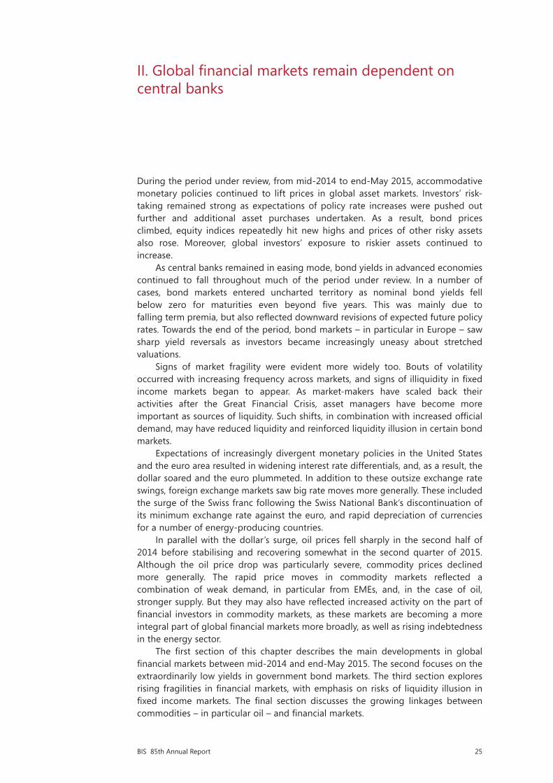
Pronounced declines in term premia played a key role in the fall in yields seen up to late April 2015. A decomposition of 10-year US and euro area bond yields into expectations of future interest rates and premia components shows that, between mid-2014 and April 2015, the estimated term premium fell by 60 basis points in the United States and by 100 basis points in the euro area (Graph II.7, left-hand panels). In the case of the United States, this was partly offset by a rise in the expectations component of about 15 basis points. This increase, in turn, was entirely due to higher expected real interest rates (plus 40 basis points), consistent with expectations of a relatively imminent lift-off of US policy rates, whereas expectations of lower inflation had a counteracting effect (minus 25 basis points; Graph II.7, top right-hand panel). As fluctuations in the expectations component in the euro area were not statistically significant, the drop in the term premium accounted for the entire fall in bond yields there (Graph II.7, bottom panels).

No doubt, central bank asset purchases played a key role in the decline of term premia and yields, reinforcing the effects of lower expected policy rates. This was especially the case in the euro area (see discussion below). Moreover, the timing of the shifts indicates that the effect of these purchases spilled over to the US bond

Falling yields, flattening curves Graph II.6

Government yield curves1 Government yield curves1 Slope of the yield curve2 Per cent Per cent Basis points

1 The dotted lines represent observations on 30 June 2014, the solid lines those on 15 April 2015. 2 Difference between the 30-year and one-year government bond yields for each country.

Source: Bloomberg.

–0.6

0.0

0.6

1.2

1.8

2.4

2y 4y 6y 8y 10yUnited StatesGermany

Mid-April 2015End-June 2014

France

–1.2

–0.6

0.0

0.6

1.2

1.8

2y 4y 6y 8y 10ySwitzerlandSweden

Denmark

Mid-April 2015End-June 2014

60

120

180

240

300

360

Q2 14 Q4 14 Q2 15United StatesGermanyJapan

ItalySpain


market, as investors chasing higher yields moved into US Treasuries (see also Chapter V).

The impact of the ECB’s expanded asset purchase programme on euro area interest rates was clearly visible. Both the programme’s announcement on 22 January 2015 and the start of the purchases on 9 March 2015 generated large price swings. The two events shifted the term structure of three-month Euribor futures downwards by up to 18 basis points, roughly corresponding to a nine-month postponement of the expected interest rate lift-off (Graph II.8, first panel). In addition, the two events pushed down 10-year German and French government bond yields by over 30 basis points.

Lower term premia influenced other long-duration assets, beyond those directly targeted by the purchases. EONIA overnight index swap (OIS) rates fell by 23 and 28 basis points for 10- and 30-year maturities, respectively (Graph II.8, second panel). Moreover, even though the ECB’s expanded purchases targeted only official sector securities, yields on euro area AAA-rated corporate bonds dropped

Falling term premia push yields lower1

In per cent Graph II.7

Ten-year bond yield Expectations component

United States

Euro area

1 Decomposition of the 10-year nominal yield according to an estimated joint macroeconomic and term structure model; see P Hördahland O Tristani, “Inflation risk premia in the euro area and the United States”, International Journal of Central Banking, September 2014. Yields are expressed in zero coupon terms; for the euro area, French government bond data are used. The shaded areas represent 90% confidence bands for the estimated components, based on 100,000 draws of the model parameter vector from its distribution at the maximum likelihood estimate and the associated covariance matrix.

Sources: Bloomberg; BIS calculations.

–1.1

0.0

1.1

2.2

3.3

2010 2011 2012 2013 2014 2015–1.1

0.0

1.1

2.2

3.3

2010 2011 2012 2013 2014 2015

–3.0

–1.5

0.0

1.5

3.0

2010 2011 2012 2013 2014 2015Ten-year bond yieldExpectations component

Term premium

0.00

0.75

1.50

2.25

3.00

2010 2011 2012 2013 2014 2015Expectations componentExpected real rate

Expected inflation


across the entire maturity spectrum, and more strongly for longer-duration bonds, as investors intensified their search for yield (Graph II.8, third panel).

The effects of central bank purchases were perhaps most obvious in the price reaction of euro area inflation-linked bonds. As the Eurosystem was getting closer to implementing its asset purchases, euro area break-even inflation rates rose significantly. Much of this increase was a direct consequence of the purchase programme rather than of higher inflation expectations: inflation swap rates rose much less, and survey measures of expected inflation remained stable. In fact, the spread between inflation swap rates and the corresponding break-even inflation rates can be viewed as an indicator of the liquidity premia in the two markets relative to nominal bonds. The typically positive spread between the two moved sharply lower, dropping 40 basis points into negative territory at the five-year maturity (Graph II.8, last panel). This suggests that in anticipation of the ECB purchases – which were explicitly announced to include index-linked bonds – investors sharply reduced their required liquidity premia on these securities, thereby pushing real yields down much more than nominal yields. This is in line with the US evidence on the Federal Reserve’s purchases of Treasury Inflation-Protected Securities (TIPS).

Central bank asset purchases have reinforced the growing weight of official holdings in government bond markets. Such holdings have increased considerably post-crisis in major economies’ government debt markets, especially for securities denominated in reserve currencies (see also Chapter V). Domestic central banks account for the lion’s share of the increase. Between 2008 and 2014, their share of the amount outstanding increased from almost 6% to more than 18%, or from $1.0 trillion to around $5.7 trillion, based on data for the United States, the euro

The ECB’s asset purchase programme has a strong effect on interest rates1 Graph II.8

Euribor futures curve change2

EONIA OIS curve change AAA corporate curve change3

Euro area inflation expectations measures3

Basis points Basis points Basis points Per cent Basis points

1 Changes from one day before to one day after the announcement of the asset purchase programme (22 January 2015) and the start of the purchases (9 March 2015). 2 Futures for March 2016, March 2017, March 2018, March 2019 and March 2020. 3 The vertical lines indicate the announcement of the ECB asset purchase programme on 22 January 2015 and the start of the purchases on 9 March 2015. 4 Based on French government bonds. 5 Based on the ECB Survey of Professional Forecasters. 6 Spread between five-year inflation swap rates and five-year break-even rates.

Sources: Bank of America Merrill Lynch; Bloomberg; Datastream; BIS calculations.

–30

–20

–10

0

2016 2017 2018 2019 202021–23 January 2015

–30

–20

–10

0

2y 5y 10y 30y 50y6–10 March 2015

–30

–20

–10

0

1–3y 3–5y 5–7y 10y+0.0

0.5

1.0

1.5

–60

–30

0

30

Q3 14 Q1 15

Rhs:

Inflation swap 5-yearBreak-even rate 5-year4

Inflation 5 years ahead5

Lhs:

Spread6


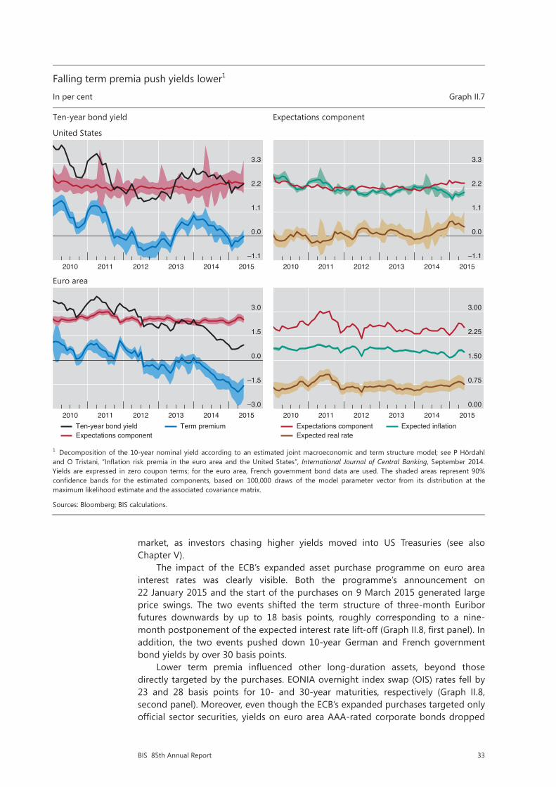
area, United Kingdom and Japan (Graph II.9, left-hand panel).1 The share of holdings by the foreign official sector has remained more stable, increasing from just above 20% to almost 22%, but the increase in absolute amounts has been sizeable, from $3.7 trillion to $6.7 trillion. On top of their holdings of government securities, official institutions have also purchased significant amounts of other debt securities. The Federal Reserve’s holdings of US agency debt securities, for example, increased by over $1.7 trillion between 2008 and 2014, while foreign official holdings declined somewhat (Graph II.9, right-hand panel).

The downward pressure on bond yields exerted by central banks and other official institutions has been reinforced by investor behaviour. In part, investors’ actions have reflected a search for yield. As bond yields further out along the maturity spectrum dropped below zero in a number of economies, investors sought still-positive yields in longer-dated bonds at the expense of duration risk. In some cases, their search for safety may also have played a role: benchmark euro area yields have tended to fall whenever concerns about the situation in Greece have intensified. And, in the background, financial regulatory reforms as well as greater demand for collateral in financial transactions have generally favoured holdings of sovereign bonds.

1 Part of these increases is due to valuation effects, as in some cases sources report market value and in others face value.

Official holdings of government securities grow1

In trillions of US dollars Graph II.9

Official holdings of government securities2 Official holdings of US Treasury and agency securities6

1 Different valuation methods based on source availability. 2 Covers the euro area, Japan, the United Kingdom and the United States; for the euro area, Japan and the United Kingdom, converted into US dollars using end-2014 constant exchange rates. 3 For the United States, total marketable Treasury securities, excluding agency debt. 4 For euro- and yen-denominated reserves, 80% is assumed to be government debt securities; for dollar-denominated reserves, as reported by the US Treasury International Capital System; for sterling-denominated reserves, holdings by foreign central banks. 5 For the euro area, national central bank holdings of general government debtand ECB holdings under the Securities Market Programme. 6 Agency debt includes mortgage pools backed by agencies and government-sponsored enterprises (GSEs) as well as issues by GSEs; total outstanding Treasury securities are total marketable Treasury securities.

Sources: ECB; Bank of Japan flow of funds accounts; Federal Reserve flow of funds accounts; IMF, COFER; UK Debt Management Office; US Department of the Treasury; Datastream; national data; BIS calculations.

0

8

16

24

32

03 04 05 06 07 08 09 10 11 12 13 14Central government debt outstanding3

Foreign official reserve holdings4

Domestic central bank holdings5

0

5

10

15

20

03 04 05 06 07 08 09 10 11 12 13 14

TreasuryTreasury and agency

Outstanding debt securities:TreasuryAgency

Foreign official holdings:

TreasuryAgency

Federal Reserve holdings:


In addition, investors’ hedging behaviour has been at work. Institutions such as pension funds and insurance companies have been under pressure to hedge the longer duration of their liabilities induced by the drop in yields. As they have sought to match the increased duration of their liabilities through purchases of long-term swaps, they have put additional downward pressure on yields and further intensified the demand for long-term fixed rates. Such behaviour highlights that institutional mandates could help generate self-reinforcing spirals in an environment where yields have been continuously pushed lower by a combination of central bank action and investor responses.

As yields dropped further below zero, concerns grew about the impact of negative rates on financial market functioning. Thus far, where negative policy rates have been imposed, these have been transmitted to money markets without major disruptions. Negative yields further out along the term structure in part reflect expectations that negative rates will prevail for some time. The longer the negative rate environment persists, the more likely it is that investors may change their behaviour, possibly in ways that are detrimental to financial market functioning.

Potential vulnerabilities can arise if institutional arrangements create a discontinuity at zero interest rates. There are several such examples. For instance, yields on most European constant net asset value funds turned negative in the first quarter of 2015, testing the effectiveness of new contractual provisions that prevent the funds from “breaking the buck”. Moreover, in some market segments, negative interest rates can complicate hedging. Some instruments, such as certain floating rate notes, set a zero floor for interest payments, either explicitly or implicitly. Hedging such instruments, or securities that depend on their cash flows, becomes problematic as standard interest rate swaps pass through negative interest payments, thereby creating a cash flow mismatch. A similar discontinuity arises if banks are unwilling to pass on negative yields to their depositors, effectively exposing themselves to additional risk if interest rates were to move further into negative territory. Chapter VI provides a more detailed analysis of the impact of negative interest rates on financial institutions.

Rising volatility puts the spotlight on market liquidity

In the past year, volatility in global financial markets began to rise from the unusually low levels that prevailed in mid-2014 (see last year’s Annual Report), spiking a few times (Graph II.10, left-hand and centre panels). The spikes, which followed years of generally declining volatility, often reflected concerns about the diverging global economic outlook, uncertainty about the monetary policy stance and fluctuations in oil prices. Investors also began to demand higher compensation for volatility risk. In particular, after narrowing until mid-2014, the gap between implied volatility and expectations of realised volatility (“volatility risk premium”) in the US equity market started to widen (Graph II.10, right-hand panel).

As risky assets such as equities and high-yield bonds were hit during these bouts of volatility, investors flocked to safe government bonds, sending their yields to new lows. The easing actions of central banks helped to quickly quell such spikes. Nevertheless, nervousness in financial markets seemed to return with increasing frequency, underscoring the fragility of otherwise buoyant markets.

A normalisation in volatility from exceptionally low levels is generally welcome. To some extent, it is a sign that investors’ risk perceptions and attitudes are becoming more balanced. That said, volatility spikes induced by little new information about economic developments highlight the impact of changing financial market characteristics and market liquidity.


Signs of market fragility after a period of declining and unusually low volatility

In percentage points Graph II.10

Implied volatilities Implied volatilities US equity volatility and risk premium5

1 Implied volatility of S&P 500, EURO STOXX 50, FTSE 100 and Nikkei 225 indices; weighted average based on market capitalisation. 2 Implied volatility of at-the-money options on commodity futures contracts on oil, gold and copper; simpleaverage. 3 Implied volatility of at-the-money options on long-term bond futures of Germany, Japan, the United Kingdom and the UnitedStates; weighted average based on GDP and PPP exchange rates. 4 JPMorgan VXY Global index. 5 Monthly averages of daily data. 6 Estimate obtained as the difference between implied and empirical volatility. 7 VIX. 8 Forward-looking estimate of empirical (or realised) volatility obtained from a predictive regression of one-month-ahead empirical volatility on lagged empirical volatility and implied volatility.


5

15

25

35

45

2010 2011 2012 2013 2014 2015Equity1

Commodity futures2

0

5

10

15

20

2010 2011 2012 2013 2014 2015Bond futures3

Exchange rates4

–20

0

20

40

60

01 03 05 07 09 11 13 15Volatility risk premium6

Implied volatility7

Empirical volatility8

There are two aspects to market liquidity. One is structural, as determined by factors such as investors’ willingness to take two-way positions and the effectiveness of order-matching mechanisms. This type of liquidity is important in quickly and efficiently dealing with transitory order imbalances. The other reflects one-sided, more persistent order imbalances, as when investors suddenly all head in the same direction. If investors persistently underestimate and underprice this second aspect, markets may appear liquid and well functioning in normal times, only to become highly illiquid once orders become one-sided, regardless of structural features.

In the wake of the financial crisis, specialised dealers, also known as market-makers, have scaled back their market-making activities, contributing to an overall reduction in the liquidity of fixed income markets. For example, the turnover ratio of US Treasuries and investment grade corporate bonds, calculated as the ratio of primary dealers’ trading volume to the amount outstanding of respective securities, has been on a declining trend since 2011. Some of the drivers for this retrenchment are related to dealers’ waning risk tolerance and reassessments of business models (Box VI.A). Others have to do with new regulations, which are aimed at bringing the costs of market-making and other trading-related activities more into line with the underlying risks and those they generate for the financial system. Finally, increasing official sector holdings of government securities may also have contributed to lower market liquidity.

Changes in market-makers’ behaviour have had varying effects on the liquidity of different bond market segments. Market-making has concentrated in the most liquid bonds. For example, market-makers in the United States have trimmed their net holdings of relatively risky corporate bonds while increasing their net US Treasury positions (Graph II.11, left-hand panel). At the same time, they have cut


the average size of relatively large trades of US investment grade corporate bonds (Graph II.11, centre panel). More generally, a number of market-makers have become more selective in offering services, focusing on core clients and markets.

As a result, there are signs of liquidity bifurcation in bond markets. Market liquidity has increasingly concentrated in the traditionally most actively traded securities, such as the government bonds of advanced economies, at the expense of less liquid ones, such as corporate and EME bonds. For example, the bid-ask spread of EME government bonds has remained high since 2012, with a large spike during the taper tantrum (Graph II.11, right-hand panel).

Even seemingly very liquid markets, such as the US Treasury market, are not immune to extreme price moves. On 15 October 2014, the yield on 10-year US Treasury bonds fell almost 37 basis points – more than the drop on 15 September 2008 when Lehman Brothers filed for bankruptcy – only to rebound by around 20 basis points within a very short period. These sharp moves were extreme relative to any economic and policy surprises at the time. Instead, an initial shock was amplified by deteriorating liquidity when a material share of market participants, who had positioned themselves for a rise in long-term rates, tried to quickly exit their crowded positions. Automated trading strategies, especially high-frequency ones, further boosted the price swings.

Another key change in bond markets is that investors have increasingly relied on fixed income mutual funds and exchange-traded funds (ETFs) as sources of market liquidity. Bond funds have received $3 trillion of investor inflows globally since 2009, while the size of their total net assets reached $7.4 trillion at the end of April 2015 (Graph II.12, left-hand panel). Among US bond funds, more than 60% of inflows were into corporate bonds, while inflows to US Treasuries remained small (Graph II.12, centre panel). Moreover, ETFs have gained importance in both advanced economy and EME bond funds (Graph II.12, right-hand panel). ETFs

Market-making and market liquidity have become more concentrated Graph II.11

US primary dealer inventory1 Average transaction size of US investment grade corporate bonds

Bid-ask spread of EME government bonds2

USD bn USD mn USD mn Basis points

1 Net dealer positions; for corporate bonds, calculated as total corporates up to April 2013 and thereafter as the sum of net positions in commercial paper, investment and below-investment grade bonds, notes and debentures and net positions in private label mortgage-backed securities (residential and commercial); for sovereign bonds, calculated as the sum of net positions in T-bills, coupons and Treasury Inflation-Indexed Securities or Treasury Inflation-Protected Securities. 2 Simple average across Bulgaria, China, Chinese Taipei, Colombia, the Czech Republic, India, Indonesia, Israel, Korea, Mexico, Poland, Romania, South Africa, Thailand and Turkey; for each country, monthly data are calculated from daily data based on a simple average across observations.

Sources: Federal Reserve Bank of New York; Bloomberg; FINRA TRACE; BIS calculations.

–200

–100

0

100

200

07 09 11 13 15CorporatesSovereign

0.05

0.06

0.07

0.08

0.09

3.6

4.2

4.8

5.4

6.0

07 09 11 13 15

<1 millionLhs:

>1 millionRhs:

0.0

3.5

7.0

10.5

14.0

10 11 12 13 14 152-year5-year

10-year


Growing importance of investors in oil markets Graph II.13

Open interest1 Money managers’ positions and the oil price Millions of barrels USD per barrel Millions of barrels

1 Crude oil, light sweet, NYMEX. 2 Weekly prices based on daily price averages from Wednesday to Tuesday.


0

750

1,500

2,250

3,000

01 03 05 07 09 11 13 15Futures Options

0

35

70

105

140

–300

–150

0

150

300

06 07 08 09 10 11 12 13 14 15

Oil price (WTI)2Lhs:

LongMoney managers’ positions (rhs):1

Short

Bond funds have grown rapidly post-crisis Graph II.12

Cumulative flows to bond funds1 Cumulative flows to US-domiciled bond funds1

Share of exchange-traded bond funds2

USD bn USD bn As a percentage of total

1 Includes mutual funds and exchange-traded funds (ETFs). 2 The ratio of cumulative flows to ETFs investing in bonds issued by advancedeconomies (or EMEs) to cumulative flows to both mutual funds and ETFs investing in bonds issued by advanced economies (or EMEs).

Sources: Lipper; BIS calculations.

0

600

1,200

1,800

2,400

3,000

09 10 11 12 13 14 15Advanced economiesEMEs

0

300

600

900

1,200

1,500

09 10 11 12 13 14 15CorporateTreasury

MortgageMunicipal

EMEOther

0

3

6

9

12

15

2010 2011 2012 2013 2014 2015Advanced economiesEMEs

promise intraday liquidity to investors as well as to portfolio managers who seek to meet inflows and redemptions without buying or selling bonds.

The growing size of the asset management industry may have increased the risk of liquidity illusion: market liquidity seems to be ample in normal times, but vanishes quickly during market stress. In particular, asset managers and institutional investors are less well placed to play an active market-making role at times of large order imbalances. They have little incentive to increase their liquidity buffers during good times to better reflect the liquidity risks of their bond holdings. And, precisely when order imbalances develop, asset managers may face redemptions by investors. This is especially true for bond funds investing in relatively illiquid corporate or EME bonds.2 Therefore, when market sentiment shifts adversely, investors may find it more difficult than in the past to liquidate bond holdings.

Central banks’ asset purchase programmes may also have reduced liquidity and reinforced liquidity illusion in certain bond markets. In particular, such programmes may have led to portfolio rebalancing by investors from safe government debt towards riskier bonds. This new demand can result in narrower spreads and more trading in corporate and EME bond markets, making them look more liquid. However, this liquidity may be artificial and less robust in the event of market turbulence.

A key question for policymakers is how to dispel liquidity illusion and support robust market liquidity. Market-makers, asset managers and other investors can take steps to strengthen their liquidity risk management and improve market transparency. Policymakers can also provide them with incentives to maintain robust liquidity during normal times to weather liquidity strains in bad times – for example, by encouraging regular liquidity stress tests. When designing stress tests, it is important to take into consideration that seemingly prudent individual actions

2 See K Miyajima and I Shim, “Asset managers in emerging market economies”, BIS Quarterly Review, September 2014, pp 19–34, and IMF, Global Financial Stability Report, April 2015, for empirical evidence.


may in fact exacerbate one-sided markets, and hence the evaporation of liquidity, if they imply similar positioning by a large number of market participants. Finally, it is vital that policymakers improve their understanding of liquidity amplification mechanisms and investor behaviour, especially in relatively illiquid markets.

Growing linkages between commodities and financial markets

The recent episode of rapidly falling oil prices has highlighted the close linkages between commodity and financial markets. Some of these linkages have been known for some time, including financial investors’ increased activity in physical commodity markets and the growth in commodity-linked derivatives markets. Others are more recent, such as commodity producers’ growing indebtedness, in particular among oil producers, and the feedback effects that this may have on commodity prices and even the dollar (Box II.B).

The nature of the production process makes commodities a natural underlying asset for derivative contracts. The extraction of oil and many other commodities requires high upfront investment, and commodity producers are exposed to considerable risks – eg weather-related risks for agricultural commodities and geopolitical risks for commodities in general. Thus, commodity producers have an interest in hedging their risks by selling their future production at a given price today (via futures and forwards) or securing a floor to that price (via options). On the other side of such contracts typically are producers of final or intermediate goods who use commodities as production inputs, or investors who want to get exposure to commodities to earn a return or diversify risk.

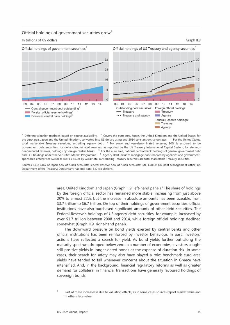
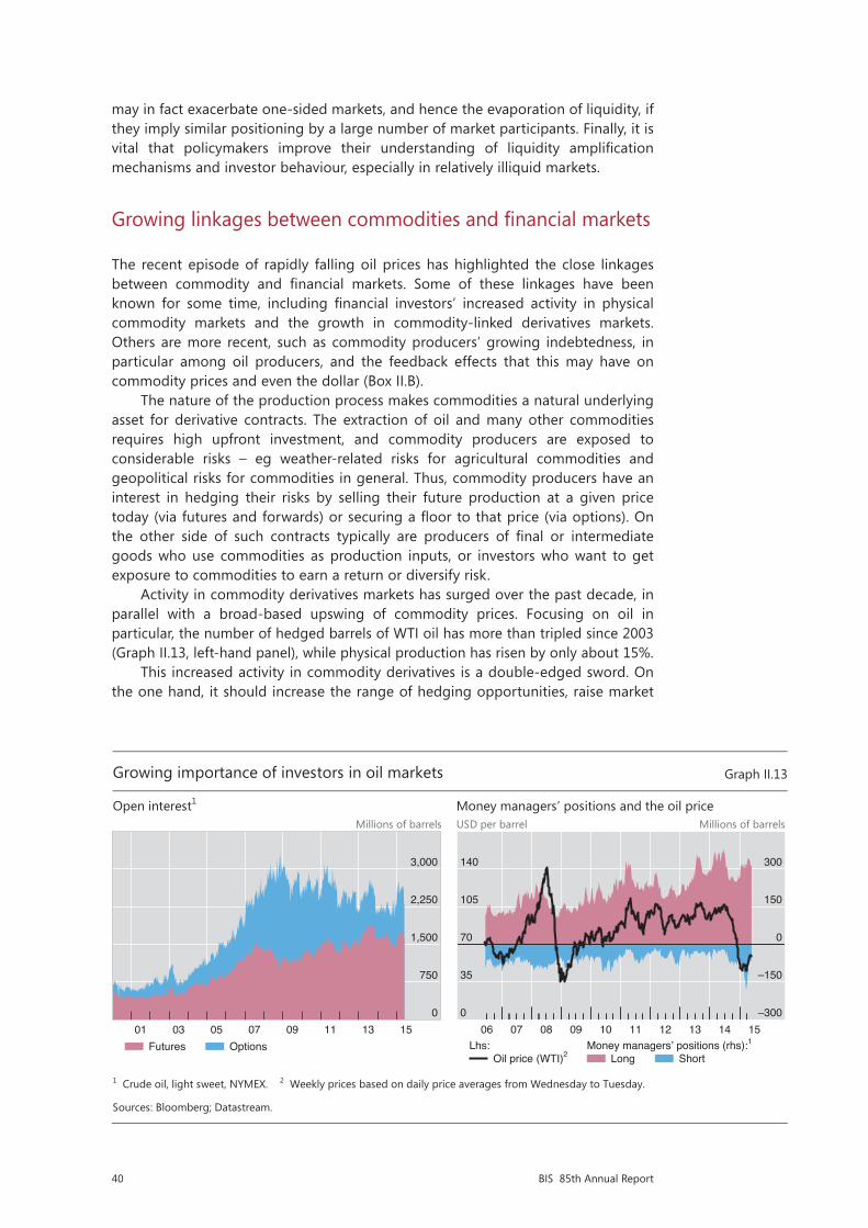
Activity in commodity derivatives markets has surged over the past decade, in parallel with a broad-based upswing of commodity prices. Focusing on oil in particular, the number of hedged barrels of WTI oil has more than tripled since 2003 (Graph II.13, left-hand panel), while physical production has risen by only about 15%.

This increased activity in commodity derivatives is a double-edged sword. On the one hand, it should increase the range of hedging opportunities, raise market

Growing importance of investors in oil markets Graph II.13

Open interest1 Money managers’ positions and the oil price Millions of barrels USD per barrel Millions of barrels

1 Crude oil, light sweet, NYMEX. 2 Weekly prices based on daily price averages from Wednesday to Tuesday.


0

750

1,500

2,250

3,000

01 03 05 07 09 11 13 15Futures Options

0

35

70

105

140

–300

–150

0

150

300

06 07 08 09 10 11 12 13 14 15

Oil price (WTI)2Lhs:

LongMoney managers’ positions (rhs):1

Short

Bond funds have grown rapidly post-crisis Graph II.12

Cumulative flows to bond funds1 Cumulative flows to US-domiciled bond funds1

Share of exchange-traded bond funds2

USD bn USD bn As a percentage of total

1 Includes mutual funds and exchange-traded funds (ETFs). 2 The ratio of cumulative flows to ETFs investing in bonds issued by advancedeconomies (or EMEs) to cumulative flows to both mutual funds and ETFs investing in bonds issued by advanced economies (or EMEs).

Sources: Lipper; BIS calculations.

0

600

1,200

1,800

2,400

3,000

09 10 11 12 13 14 15Advanced economiesEMEs

0

300

600

900

1,200

1,500

09 10 11 12 13 14 15CorporateTreasury

MortgageMunicipal

EMEOther

0

3

6

9

12

15

2010 2011 2012 2013 2014 2015Advanced economiesEMEs


Box II.BWhat drives co-movements in the oil price and the dollar?

The sharp appreciation of the US dollar and the rapid fall in the oil price are two of the most noteworthy market developments of the past year. As argued in this chapter, diverging monetary policies played a key role in the dollar’s strength, whereas a combination of increasing supply, falling demand and market-specific factors were important in explaining the oil price drop. It is less clear, however, to what extent the two phenomena are linked. This box discusses some of the possible links.

The relationship between the trade-weighted US dollar exchange rate and the price of crude oil has changed over time (Graph II.B, left-hand panel). Evidence from before the 1990s points to a positive correlation. The reason is unclear. One argument is that oil exporters spent a large share of oil revenues on US goods, which had a tendency to improve the US trade balance, and hence to boost the dollar exchange rate, when oil became more expensive. Accordingly, as the share of oil producers’ imports from the United States declined relative to the US share in their oil exports, this channel became less potent. Another possible explanation is that a worsening economic outlook in the United States would typically result in a weaker currency and a lower demand for oil. This channel, too, would have become weaker as the US share in global output declined.

Since the early 2000s, a stronger US dollar exchange rate has gone hand in hand with a lower oil price, and vice versa (Graph II.B, left-hand and centre panels). The prominent role of the US dollar as invoicing currency for commodities is one possible explanation: oil producers outside the United States may adjust the dollar price of oil in order to stabilise their purchasing power. At the same time, increasing investment activity in oil futures and options may also play a role. The monetary policy stance of the Federal Reserve or flight to safety episodes that naturally influence the US dollar exchange rate may also affect financial investors’ risk-taking, prompting them to move out of oil as an asset class when the US dollar becomes a safe haven currency and into oil when they are willing to take on more risk. Consistent with this view, the right-hand panel of Graph II.B illustrates the increasingly strong negative relationship between oil prices and financial investors’ risk aversion, as measured by the VIX index.

Another financial channel could reflect the attributes of oil as both the main source of income and an asset backing the liabilities of oil producers. For example, when the oil price stayed high, EME firms borrowed, sometimes heavily, to invest in oil extraction, with oil stocks acting as implicit or explicit collateral in these debt contracts. As

Tight links between oil, the dollar and financial markets Graph II.B

Oil and the dollar1 Oil investor activity and oil-dollar correlation4

Oil and volatility index6

Millions of barrels

1 Average of values across the month. 2 In US dollars per barrel. 3 BIS nominal effective exchange rate narrow index; a decline (increase) indicates depreciation (appreciation) of the US dollar in trade-weighted terms. 4 Correlation calculated by using Engle’s (2002) Dynamic Conditional Correlation GARCH model. 5 Crude oil, light sweet, NYMEX. 6 One-month differences.


0

25

50

75

100

125

100 120 140 160 180 200

Oil

pric

e (W

TI)2

USD nominal effective exchange rate3

1983–99 2000 onwards

0

600

1,200

1,800

2,400

3,000

–0.4

–0.3

–0.2

–0.1

0.0

0.1

00 02 04 06 08 10 12 14Lhs:Rhs:

Total open interest5

Oil price (WTI)2 and USD nominal effective exchange rate correlation3

–32

–24

–16

–8

0

8

–10 0 10 20 30 40 50

R2 = 0.02

R2 = 0.10 Oil

pric

e (W

TI)2

VIX1986–99 2000 onwards


access to credit and collateral prices are closely linked, the fall in oil prices eroded oil producers’ profits and simultaneously tightened their financing conditions. This would induce firms to hedge or cut their dollar liabilities, thereby increasing the demand for dollars. The strong negative relationship between oil prices and spreads on high-yield debt of oil producers is consistent with this view.

See R Amano and S van Norden, “Oil prices and the rise and fall of the US real exchange rate”, Journal of International Money and Finance, vol 17(2), April 1998. See M Fratzscher, D Schneider and I van Robays, “Oil prices, exchange rates and asset prices”, ECB Working Papers, no 1689, July 2014. See D Domanski, J Kearns, M Lombardi and H S Shin, “Oil and debt”, BIS Quarterly Review, March 2015, pp 55–65.

liquidity, reduce price volatility, and more generally improve the price formation mechanism, at least in normal times. On the other hand, investors’ decisions are subject to rapidly shifting expectations about price trends and fluctuations in risk appetite and financing constraints. This may induce them to withdraw from the market at times of losses and heightened volatility (Graph II.13, right-hand panel).

Bigger and more liquid commodity futures markets mean that commodity prices tend to react more quickly and strongly to macroeconomic news. Changes in commodity investor sentiment often seem to be largely driven by the general macroeconomic outlook, rather than by commodity-specific factors. This could also explain the recent stronger co-movements in commodity and equity prices. The extent to and speed with which arbitrage opportunities can be exploited between the physical and futures markets are critical to price formation. They influence the degree to which fluctuations in futures prices transmit to the prices commodity producers charge and, vice versa, the degree to which changes in the consumption and production of a given commodity are reflected in futures prices (Box II.A).

Rising energy sector debt and widening spreads Graph II.14

US corporate bonds outstanding1 EME corporate bonds outstanding2 High-yield US corporate bond spreads3

USD bn USD trn USD bn USD trn Basis points

1 Face value of Merrill Lynch high-yield and investment grade corporate bond indices. 2 Face value; energy sector includes oil & gas and utility & energy firms; bonds issued in US dollars and other foreign currency by firms based in Brazil, Bulgaria, Chile, China, Colombia, the Czech Republic, Estonia, Hong Kong SAR, Hungary, India, Indonesia, Israel, Korea, Latvia, Lithuania, Mexico, Peru, the Philippines, Poland, Romania, Russia, Singapore, Slovenia, South Africa, Thailand, Turkey and Venezuela. 3 Option-adjusted spread over US Treasury notes.

Sources: Bank of America Merrill Lynch; Bloomberg; Dealogic.

Physical and futures prices of oil co-move closely

In US dollars per barrel Graph II.A

Price of oil and refiners’ acquisition costs WTI oil futures strips

1 Refiners’ acquisition cost of domestic and imported crude oil.


0

140

280

420

560

700

840

0.0

1.8

3.6

5.4

7.2

9.0

10.8

07 09 11 13 15

EnergyLhs:

All sectorsRhs:

0

60

120

180

240

300

360

0.0

0.2

0.4

0.6

0.8

1.0

1.2

07 09 11 13 15

EnergyLhs:

All sectorsRhs:

0

350

700

1,050

1,400

1,750

2,100

07 09 11 13 15All sectors Energy

20

40

60

80

100

120

2009 2010 2011 2012 2013 2014 2015Brent WTI Refiners’ acquisition costs1

20

40

60

80

100

120

2009 2010 2011 2012 2013 2014 20153-month 24-month Dec 2019 contract


Oil producers’ easier access to financing has sharply boosted indebtedness in the sector. The persistently high prices recorded over recent years made it profitable to exploit alternative sources of oil, such as shale oil and deep-water sources. To reap hefty expected profits, oil firms boosted investment, in many cases through debt. The amount outstanding of bonds issued by US and EME energy firms, including oil and gas companies, has more or less quadrupled since 2005, growing at a much faster pace than in other sectors (Graph II.14, left-hand and centre panels).

After the recent sharp oil price fall, the oil sector’s high indebtedness has exacerbated the rise in financing costs. Indeed, energy firms’ bond yields soared when oil prices plummeted (Graph II.5, left-hand and centre panels). And bond yields of US energy firms in the high-yield segment, which had normally been lower than those of other sectors, rose well above them (Graph II.14, right-hand panel).

High indebtedness may, in addition, have amplified the oil price drop. As oil prices fell, energy firms’ refinancing costs rose and their balance sheets weakened. Rather than cutting back production, some firms may have tried to preserve cash flows by boosting output and/or selling futures in an attempt to lock in prices. In line with this, oil production in the United States, including shale oil extraction, remained strong as oil prices fell, leading to a rapid build-up in the levels of crude oil in US storage up to the first quarter of 2015.3

3 See D Domanski, J Kearns, M Lombardi and H S Shin, “Oil and debt”, BIS Quarterly Review, March 2015, pp 55–65, for further details and evidence.

global financial markets remain dependent on central banks

Documents