global estimates of seafloor slope from single-beam ship...

Global estimates of seafloor slope from single-beam

ship soundings

Joseph J. Becker1 and David T. Sandwell1

Received 13 August 2006; revised 7 January 2008; accepted 28 February 2008; published 30 May 2008.

[1] Rough topography on the ocean floor is a source of ocean mixing which is of interestto both physical oceanography and climate science. Most mixing has been attributed tohigh slopes of the large-scale structures of the deep ocean floor such as seamounts,continental margins, and mid-ocean ridge axes. In this paper, we show the small-scalebut ubiquitous abyssal hills and fracture zones dominate the global map of roughtopography. Much of this rugged seafloor occurs in the Southern Ocean on the flanks ofthe Pacific-Antarctic Rise and Southwest Indian Ridge. We present our results as aglobal map of the mean slope of the ocean floor, and as a global map of the oceanfloor above the M2 critical slope. We compare our results to multibeam and satellitebathymetry data to show that satellite bathymetry is not a valid proxy for multibeammeasurements, but edited single-beam sonar data are adequate to provide a globalperspective on features with horizontal wavelengths as small as 2 km.

Citation: Becker, J. J., and D. T. Sandwell (2008), Global estimates of seafloor slope from single-beam ship soundings, J. Geophys.

Res., 113, C05028, doi:10.1029/2006JC003879.

1. Introduction

[2] In a classic paper, Munk [1966] assumed constantupwelling and estimated the eddy diffusivity needed tomaintain the observed abyssal ocean stratification as wellas the amount of energy needed to mix the abyssal ocean.The O(10�4 m2/sec) diffusivity [Munk, 1966] predicted wasnot found experimentally [c.f. Osborn, 1980]. Eddy diffu-sivity is difficult to measure, but with the semiempiricalmethods of Osborn [Osborn, 1980; Osborn and Cox, 1972]and Dillon [1982], reliable experimental results wereobtained. Recent measurements show that mixing is en-hanced by orders of magnitude near rough topography[Nash et al., 2007; Polzin et al., 1997; Toole et al., 1997].Munk and Wunsch [1998] addressed the missing diffusivityin the mid ocean and the increased mixing over roughtopography by proposing that tidal dissipation was a powersource of mixing and mixing preferentially occurred wheninternal tides flowed across steep slopes. There is anextensive body of experimental, theoretical, and numericalresearch on the production of internal waves by the inter-action of tidal currents with variable topography [cf. Garrettand Kunze, 2007]. Baines [1982] examined the simple caseof horizontal tidal excursions impinging on a uniformcontinental slope and found that for semidiurnal tides in astably stratified layer, there is a critical slope where con-version of the barotropic tide is most efficient. In the deepocean where the stratification is low, this critical slope

ranges from 0.1 to 0.3 m/m so only very steep topographycan generate internal waves in this simplified model.Llewellyn Smith and Young [2002] extended the model toshow the shape of the topographic spectrum determines theamount of energy conversion in an ocean of finite depthwith arbitrary stratification.[3] Satellite altimetry has been used to measure the

global barotropic tide [Kantha, 1995], as well as thelocation and magnitude of its global dissipation [Egbertand Ray, 2000, 2001, 2003]. The global dissipation studiesindicated that the approximately 1/3 of the semidiurnalbarotropic tidal dissipation occurs in the deep oceans,apparently over the mid-ocean ridges (MOR) and sea-mounts. However, the dissipation maps do not have suffi-cient spatial resolution to provide a clear correlation withseafloor structures [Egbert and Ray, 2003]. The lackof resolution reflects the wide track spacing of TOPEX/POSEIDON altimeter profiles (�150 km) as well as thesubtlety and difficulty of the measurements presented byEgbert and Ray [2003].[4] In this paper, we present the global spatial distribution

of seafloor slope and roughness in the abyss (depth >2000m).In particular, we focus on abyssal hills and fracture zonesthat extend over large parts of the ocean basins, especiallyon the lightly sedimented flanks of the slower spreadingridges. If, as proposed by Ledwell et al. [2000], most of thetidal dissipation in the deep ocean occurs on abyssal hills,mapping their global distribution is important. We alsoshow a significant fraction of seafloor (4.5%) has slopegreater than the M2 critical slope. Much of this super criticalseafloor occurs in the Southern Ocean on the flanks of thePacific-Antarctic Rise and Southwest Indian Ridge. Thesehigh-slope facets have either not been detected before, orhave been grossly underestimated because satellite bathym-

JOURNAL OF GEOPHYSICAL RESEARCH, VOL. 113, C05028, doi:10.1029/2006JC003879, 2008ClickHere

for

FullArticle

1Institute of Geophysics and Planetary Physics, Scripps Institution ofOceanography, La Jolla, California, USA.

Copyright 2008 by the American Geophysical Union.0148-0227/08/2006JC003879$09.00

C05028 1 of 14

http://dx.doi.org/10.1029/2006JC003879

etry [Smith and Sandwell, 1997] does not resolve featureshaving horizontal scales less than 10 km.

2. Global Estimate of Critical Slope

[5] While we are considering a more complete spectralanalysis of the sounding data, a great deal can be learnedfrom a simple ‘‘critical slope’’ analysis. The internal tideliterature [Baines, 1982] describes topography as beingeither super or sub critical. A well-known approximationfor the critical slope of the topography is [Baines, 1982]

a2 � tan2 qg� �

¼ w2 � f 2ð ÞN2 � w2ð Þ ; ð1Þ

where qg is the angle between the group velocity vector andthe horizon, w is the frequency of internal wave (radian/sec)generated by the M2 tide, f is the inertial frequency and N isthe buoyancy frequency. For waves of given frequency(always M2 in this paper) at given latitude the onlyunknown is the buoyancy frequency which depends onthe density profile,

N2 ¼ �g

r@r@z

� g2

c2� �g

r@rq@z

ð2Þ

where z is the vertical coordinate, c is the speed of sound, ris the in situ density, rq the potential density, and g is theacceleration of gravity (9.8 m/s2) [Knauss, 1997].[6] A detailed global density profile is unavailable. We

calculate an approximate buoyancy frequency profile usingthe CSIRO MATLAB routines [Morgan and Pender, 2003]at every depth and location in the 1� World Ocean Atlas(WOA) [Conkright et al., 2007]. Noise in the WOA valuesof temperature and salinity made the calculated values of N2

noisy and occasionally negative. To stabilize our estimate ofN, we first removed negative values of N2 and other obviouserrors, and then followed St Laurent and Garrett [2002] byfitting N to an exponential function of depth.

ln Nð Þ ¼ c0 þ c1z: ð3Þ

[7] For depths that exceed the maximum depth in theWOA, we simply assumed N changes only slightly atabyssal depths, and used the deepest WOA depth at thatlocation rather than extrapolate a fit to very noisy data. Thecalculated critical slope has at least two significant sourcesof error. First, the value of N is based on the WOA andwhich is an empirical data set with the usual potential forrandom and systematic errors. Second, our N is an empiricalfit to an exponential of depth [St. Laurent and Garrett,2002]; the truth is substantially more complex. As a result,our critical slope calculation is a semiqualitative result.[8] To test the accuracy of our critical slope calculation

we compared it to CTD data from two WOCE cruises.Appendix 1 is a comparison of our fit to the WOA data andWOCE CTD data along a meridian at 150W between Alaskaand Antarctica. We find good agreement between the criticalslope estimates from these two independent data sets sug-gesting that the WOA data is adequate for this globalanalysis.

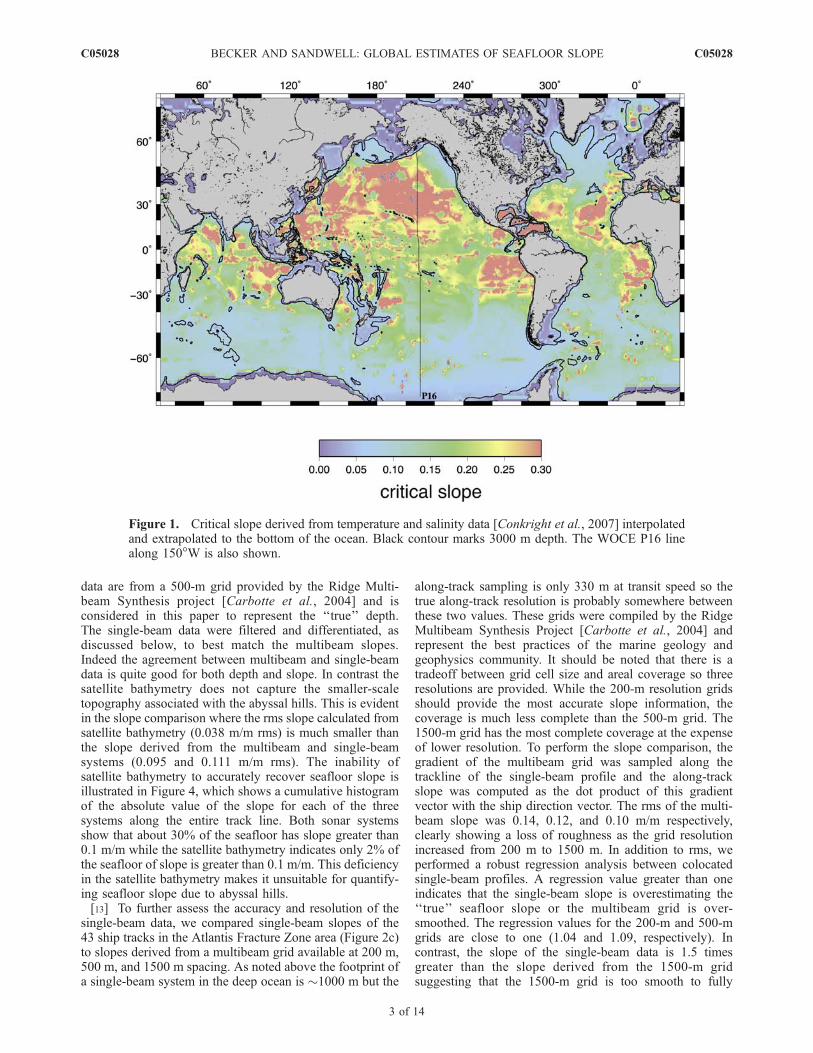
[9] The global map of critical slope based on work byConkright et al. [2007] is shown in Figure 1. The mapextends only to ±72�, so the M2 turning latitudes at 75� arenot visible. The latitudinal trend toward a critical slope ofzero at those turning latitudes is apparent, as is the generaldecrease of N (increasing critical slope) with increasingdepth. Low critical slope occurs on the shallow continentalmargins, the crests of seamounts such as the Hawaiianridge, and along the mid-ocean ridges with depths between2000 and 3000 m. There is a prominent asymmetry betweenthe North and South Pacific, east-west asymmetries in theSouth Atlantic, across the equatorial East Pacific Rise, andacross the Ninety-East Ridge in the Indian Ocean. Thisasymmetry is also seen in the WOCE CTD analysis pro-vided in Appendix A.

3. Satellite Bathymetry Greatly UnderestimatesSeafloor Roughness

[10] The slope of the ocean floor depends on the lengthscale of interest since, for example, individual pillow basaltscan have vertical sides. The critical slope theory assumesthat the length scale of the topography is greater than thetidal excursions of �200 m [Garrett and Kunze, 2007]. Atypical single-beam echo sounder has a beam width of �15�so in the deep ocean (4000 m) it insonofies a zone about1000 m across. Higher resolution (�200 m) is possible withmodern multibeam systems but much of that data is col-lected at transit velocities, which limits the resolution toseveral hundred meters.[11] Three types of measurement systems are used to map

the topography and roughness of the ocean floor. Single-beam echo sounders, widely used since the 1960s, provideprofile of depth from thousands of research cruises(Figure 2). While coverage is widespread, there are gapsas large as 200 km by 200 km, especially in the SouthernOcean. Multibeam echo sounding, available on most largeresearch vessels since the mid 1990s, map 5–20 km wideswaths of seafloor at a horizontal resolution that depends onthe depth of the water; 200–500 m at 4 km depth dependingon ship speed and swath width. Ideally, the world’s oceansshould be exhaustively measured with multibeam bathym-etry, but only a small percentage of the ocean floor has beenso measured [Smith and Sandwell, 2004]. The third ap-proach combines the sparse ship soundings with densesatellite-derived gravity anomalies to estimate depth androughness [Gille et al., 2000; Smith and Sandwell, 1997].Satellite bathymetry can only resolve features with wave-lengths between 20 and 160 km and misses most, if not all,of the small-scale roughness associated with the abyssalhill fabric. While none of these three measurementsystems provides global coverage at the scales of interest(2–200 km), we show that the along-track analysis of thesingle beam provides an acceptable compromise betweencoverage and resolution if abyssal hills are assumed to besmoothly varying in slope over distances greater than a fewhundred kilometers [Goff, 1991].[12] To assess the accuracy and resolution capabilities of

each of the three systems, we compared multibeam, single-beam, and satellite bathymetry along the track of an error-free, but otherwise typical cruise near the Atlantis TransformFault on the Mid Atlantic Ridge (Figure 3). The multibeam

C05028 BECKER AND SANDWELL: GLOBAL ESTIMATES OF SEAFLOOR SLOPE

2 of 14

C05028

data are from a 500-m grid provided by the Ridge Multi-beam Synthesis project [Carbotte et al., 2004] and isconsidered in this paper to represent the ‘‘true’’ depth.The single-beam data were filtered and differentiated, asdiscussed below, to best match the multibeam slopes.Indeed the agreement between multibeam and single-beamdata is quite good for both depth and slope. In contrast thesatellite bathymetry does not capture the smaller-scaletopography associated with the abyssal hills. This is evidentin the slope comparison where the rms slope calculated fromsatellite bathymetry (0.038 m/m rms) is much smaller thanthe slope derived from the multibeam and single-beamsystems (0.095 and 0.111 m/m rms). The inability ofsatellite bathymetry to accurately recover seafloor slope isillustrated in Figure 4, which shows a cumulative histogramof the absolute value of the slope for each of the threesystems along the entire track line. Both sonar systemsshow that about 30% of the seafloor has slope greater than0.1 m/m while the satellite bathymetry indicates only 2% ofthe seafloor of slope is greater than 0.1 m/m. This deficiencyin the satellite bathymetry makes it unsuitable for quantify-ing seafloor slope due to abyssal hills.[13] To further assess the accuracy and resolution of the

single-beam data, we compared single-beam slopes of the43 ship tracks in the Atlantis Fracture Zone area (Figure 2c)to slopes derived from a multibeam grid available at 200 m,500 m, and 1500 m spacing. As noted above the footprint ofa single-beam system in the deep ocean is �1000 m but the

along-track sampling is only 330 m at transit speed so thetrue along-track resolution is probably somewhere betweenthese two values. These grids were compiled by the RidgeMultibeam Synthesis Project [Carbotte et al., 2004] andrepresent the best practices of the marine geology andgeophysics community. It should be noted that there is atradeoff between grid cell size and areal coverage so threeresolutions are provided. While the 200-m resolution gridsshould provide the most accurate slope information, thecoverage is much less complete than the 500-m grid. The1500-m grid has the most complete coverage at the expenseof lower resolution. To perform the slope comparison, thegradient of the multibeam grid was sampled along thetrackline of the single-beam profile and the along-trackslope was computed as the dot product of this gradientvector with the ship direction vector. The rms of the multi-beam slope was 0.14, 0.12, and 0.10 m/m respectively,clearly showing a loss of roughness as the grid resolutionincreased from 200 m to 1500 m. In addition to rms, weperformed a robust regression analysis between colocatedsingle-beam profiles. A regression value greater than oneindicates that the single-beam slope is overestimating the‘‘true’’ seafloor slope or the multibeam grid is over-smoothed. The regression values for the 200-m and 500-mgrids are close to one (1.04 and 1.09, respectively). Incontrast, the slope of the single-beam data is 1.5 timesgreater than the slope derived from the 1500-m gridsuggesting that the 1500-m grid is too smooth to fully

Figure 1. Critical slope derived from temperature and salinity data [Conkright et al., 2007] interpolatedand extrapolated to the bottom of the ocean. Black contour marks 3000 m depth. The WOCE P16 linealong 150�W is also shown.


3 of 14

C05028

capture seafloor slope at a wavelength of 2 km. Thesecomparisons demonstrate that the along-track slope derivedfrom a single-beam profile is similar in amplitude to the bestmultibeam grids at 200-m and 500-m resolution.[14] While single-beam slope measurements are close to

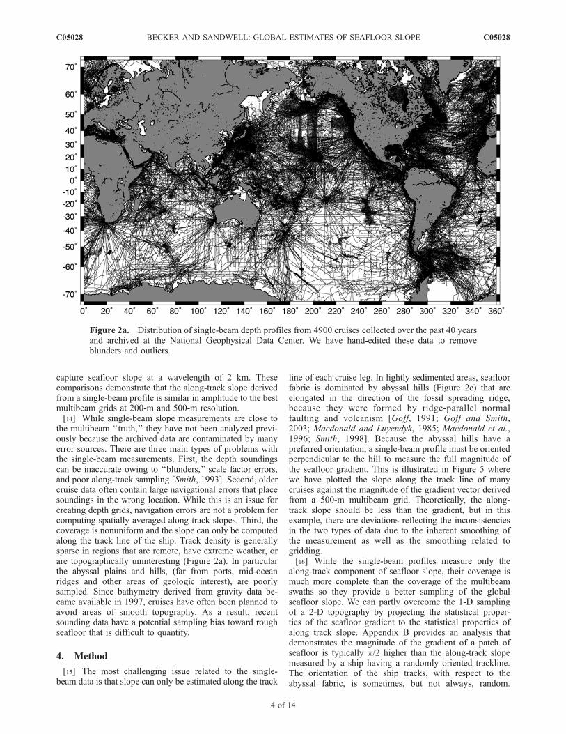
the multibeam ‘‘truth,’’ they have not been analyzed previ-ously because the archived data are contaminated by manyerror sources. There are three main types of problems withthe single-beam measurements. First, the depth soundingscan be inaccurate owing to ‘‘blunders,’’ scale factor errors,and poor along-track sampling [Smith, 1993]. Second, oldercruise data often contain large navigational errors that placesoundings in the wrong location. While this is an issue forcreating depth grids, navigation errors are not a problem forcomputing spatially averaged along-track slopes. Third, thecoverage is nonuniform and the slope can only be computedalong the track line of the ship. Track density is generallysparse in regions that are remote, have extreme weather, orare topographically uninteresting (Figure 2a). In particularthe abyssal plains and hills, (far from ports, mid-oceanridges and other areas of geologic interest), are poorlysampled. Since bathymetry derived from gravity data be-came available in 1997, cruises have often been planned toavoid areas of smooth topography. As a result, recentsounding data have a potential sampling bias toward roughseafloor that is difficult to quantify.

4. Method

[15] The most challenging issue related to the single-beam data is that slope can only be estimated along the track

line of each cruise leg. In lightly sedimented areas, seafloorfabric is dominated by abyssal hills (Figure 2c) that areelongated in the direction of the fossil spreading ridge,because they were formed by ridge-parallel normalfaulting and volcanism [Goff, 1991; Goff and Smith,2003; Macdonald and Luyendyk, 1985; Macdonald et al.,1996; Smith, 1998]. Because the abyssal hills have apreferred orientation, a single-beam profile must be orientedperpendicular to the hill to measure the full magnitude ofthe seafloor gradient. This is illustrated in Figure 5 wherewe have plotted the slope along the track line of manycruises against the magnitude of the gradient vector derivedfrom a 500-m multibeam grid. Theoretically, the along-track slope should be less than the gradient, but in thisexample, there are deviations reflecting the inconsistenciesin the two types of data due to the inherent smoothing ofthe measurement as well as the smoothing related togridding.[16] While the single-beam profiles measure only the

along-track component of seafloor slope, their coverage ismuch more complete than the coverage of the multibeamswaths so they provide a better sampling of the globalseafloor slope. We can partly overcome the 1-D samplingof a 2-D topography by projecting the statistical proper-ties of the seafloor gradient to the statistical properties ofalong track slope. Appendix B provides an analysis thatdemonstrates the magnitude of the gradient of a patch ofseafloor is typically p/2 higher than the along-track slopemeasured by a ship having a randomly oriented trackline.The orientation of the ship tracks, with respect to theabyssal fabric, is sometimes, but not always, random.

Figure 2a. Distribution of single-beam depth profiles from 4900 cruises collected over the past 40 yearsand archived at the National Geophysical Data Center. We have hand-edited these data to removeblunders and outliers.


4 of 14

C05028

Seagoing expeditions not focused on seafloor geology, orcruises in transit across the basins, sample the abyssalfabric in an essentially random direction. However, acruise focused on geology and geophysics is typically

preferentially oriented perpendicular or parallel to theabyssal fabric (e.g., Figure 2a, bottom). Because of thispossible sampling direction bias, we report mean slope

Figure 2b. Distribution of single-beam (black) and multibeam (red) echo soundings in the NorthAtlantic. Gray box shows area where single-beam, multibeam, and satellite bathymetry measurementswere compared.

Figure 2c. Multibeam grid (500-m cell size) over the Mid-Atlantic Ridge and Atlantis Fracture Zone.Track lines are the single-beam or center-beam coverage used to relate 2-D gradients to 1-D slopes.


5 of 14

C05028

Figure 3. Seafloor (top) depth and (bottom) along-track slope along the trackline of a typical cruise nearthe Mid-Atlantic Ridge (MAR). Multibeam data were sampled from a grid having 500-m cell spacing andrepresent the ‘‘true’’ depth and slope. Single-beam data were filtered and processed along track to bestmatch the multibeam profile. This version of satellite bathymetry was not forced to agree with availablesoundings so is representative of the accuracy in areas having no shipboard coverage. The rms differencesare: single-beam depth 48.4 m, satellite bathymetry 190.8 m, single-beam slope 0.066 m/m, andmultibeam slope 0.089 m/m.

Figure 4. Cumulative histograms of the absolute value of the seafloor slope along the trackline from thethree measurement systems. Thirty percent of the multibeam and single-beam slopes exceed 0.1 m/m,while only 2% of satellite bathymetry slopes exceeds 0.1 m/m.


6 of 14

C05028

without scaling up by p/2. This conservative approachunderstates the extent of supercritical seafloor.

5. Data Processing

[17] The examples provided so far have used single-beamdata that are not contaminated by errors in depth or naviga-tion. Approximately 1/3 of the 4900 cruise legs of single-beam bathymetry data available from the GEODAS database[National Geophysical Data Center, 2006] have significanterrors. These 1800 cruises have never been used in the globalsatellite bathymetry maps [Smith and Sandwell, 1997] eventhough, in many cases, the entire month-long set of depthsoundings had only a few outliers. The automatic algorithmused to screen out obviously bad cruises generally failed toidentify the occasional bad pings in good cruises becausethe types of errors are so diverse. Typical errors include:navigation errors, digitizing errors, typographical errors dueto hand entry of older sounding, reporting the data infathoms instead of meters, incorrect sound speed measure-ments, and even computer errors in reading punch cards[Smith, 1993]. Just one bad section of a cruise in an isolatedregion introduces a seafloor topographic feature that doesnot exist and the entire cruise is rejected.[18] About 5000 cruises of single-beam soundings col-

lected over the past 40 years and archived at the NationalGeophysical Data Center [2006] have been hand edited bycomparing measured depth to satellite bathymetry (i.e.,based on gravity only). These data will be combined withmultibeam data to refine the global satellite bathymetry grid[Smith and Sandwell, 1997] and create a new global grid at1 km resolution. This involved the development of agraphical user interface program consisting of three linkedwindows, the ship track, the along track profile, and ascatter diagram of altimetric versus measured depth. Typicalrms differences between the measured and satellite bathym-etry are 250 m. We expect the rms errors in the soundings tobe less than 25 m [Smith, 1993] so most of the badsoundings are obvious outliers. The analyst scans the profiledata for large deviations from the satellite bathymetry(typically > 500 m) and flags these data as being suspect.The edited cruise is returned to the database with the suspectdata flagged. Using this tool, we have edited the approxi-mately 30 million pings from the GEODAS database.[19] These clean data were then low-pass filtered and

differentiated along track to estimate seafloor slope asdiscussed below using the software tools in GMT [Wesseland Smith, 1995]. The ship track profiles were prefilteredwith a Gaussian low-pass filter having a 0.5 gain at awavelength of 2 km. The 2-km filter is partly motivatedby the expected beam width of single-beam sonar (�1 km)in the deep ocean (W. H. F. Smith, personal communication,2005). Ship track data are unequally spaced; for example,the ship speed changes, but the ping rate is relativelyuniform. Moreover, the spacing of the older hand-digitizeddata is based on the seafloor features. For example, flatabyssal plains sometimes have 4-km spacing betweensoundings because the human digitizer determined that afiner spacing was unnecessary. This uneven and sometimeslarge spacing does not strictly support a 2-km wavelengthresolution. We selected this resolution as a compromisebecause the widely spaced older soundings presumably

would have a smaller spacing if the human digitizer felt itwas needed to capture the actual seafloor slope. After low-pass filtering, the data were differentiated along track at aminimum interval of 1/4 the wavelength of the low-passfilter (500 m). More complex signal processing is notneeded when the ship track data is correctly edited.[20] The calculation of the fraction of seafloor above

critical slope discussed below was done in three steps inorder to minimize the bias due to the uneven distribution ofship soundings. First, we created two 0.1� longitude by 0.1�latitude grids, one consisting of the total number of slopeestimates in each grid cell and a second consisting of thenumber of slope estimates (absolute value) that exceed thecritical slope in each grid cell. Second, these two grids werelow-pass filtered with a radial Gaussian filter (s = 10 km) todetermine the number of slopes per 628 km2; the integratedarea under a radial Gaussian is 2ps2. Third, the fraction ofseafloor with slope above the critical slope was computed asthe ratio of the two grids. Areas with less than one ping per100 km2 were not used to avoid taking the ratio of verysmall numbers. For display purposes, the fraction of sea-floor above critical slope is median filtered and interpolatedonto a 1� grid (Figure 7a). This process combines theinformation in Figures 6 and 7.

6. Global Measurement of Seafloor Roughness

[21] The global map of spatially averaged seafloor slopeis shown in Figure 6. Along-track slopes were binned in a0.25� longitude by 0.2� latitude intermediate grid and themean slope was calculated for each bin. The binning is doneto reduce the bias due to uneven sampling by the shipsoundings. In particular, the ridge axes are sampled muchmore densely than the abyssal plains. We find that seafloor

Figure 5. Magnitude of along-track slope of the seafloorfrom single-beam data (Figure 3, bottom) versus magnitudeof gradient vector at the same locations from a 500-mmultibeam grid. Theoretically the 1-D slope should be lessthan or equal to the 2-D gradient.


7 of 14

C05028

slope varies more than an order of magnitude throughoutthe deep oceans and depends on a combination of tectonicand sedimentary processes. Large-scale features (>40 km)such as continental margins, ridge axes, fracture zones,trenches, and seamounts are sometimes associated withslope greater than 0.05. These large-scale features arewell resolved in bathymetry derived from satellite-derivedgravity anomalies and sparse ship soundings [Smith andSandwell, 1997]. Such maps have been band-pass filteredbetween 20 and 160 km wavelength to reveal the slope androughness of the seafloor and to relate these bottom char-acteristics to mesoscale variability [Gille et al., 2000] andocean mixing [Jayne and St Laurent, 2001].[22] Using only ship soundings, we find that the global

mean slope map is dominated by the distribution of thesmaller-scale abyssal hill topography and fracture zones.Abyssal hills are generated at mid-ocean ridges by acombination of volcanism and normal faulting [Cannat etal., 2006; Lonsdale, 1977; Macdonald and Luyendyk,1985]. The amplitude and wavelength of abyssal hillsdepends strongly on the rate of seafloor spreading [Goff,1991; Goff et al., 2004; Kunze and Llewellyn Smith,2004] that also controls the morphology of the spreadingridge axis where they were formed [Canuto et al., 2004;Macdonald, 1982; Macdonald et al., 1988; Menard, 1967;Small and Sandwell, 1992]. On older seafloor, a thick layer

of sediment often covers the abyssal fabric. Sedimentedseafloor can be extremely flat at the scale of abyssal hills. Insummary, there are basin-scale variations in seafloor slopethat are well explained in terms of variations in seafloorspreading rate and the thickness of the sediments. Thesespatial variations in slope occur over distances greater thana few hundred kilometers [Goff and Jordan, 1989] so thesparse track sampling in the Southern Ocean (�40 km trackspacing) is adequate for characterizing global seafloorslope.

7. Fraction of Seafloor Above Critical Slope

[23] Given the slope along each ship track and the criticalslope interpolated to the same location we calculate thefraction of seafloor having slope above the critical slope.This calculation is allows us to estimate the total area ofsuper critical seafloor. It is also useful because it at leastpartially addresses the issue of mixing hot spots. [Nash etal., 2007] suggest that mixing in the deep ocean is localizedin a few small areas. Therefore, an area’s potential formixing may not be the average critical slope, but thefraction of the area that is super critical.[24] For comparison, we performed a similar analysis

using the global 2-min grid of Smith and Sandwell [1997](Figure 7b). Since the full gradient of the Smith and

Figure 6. Mean slope of the seafloor filtered with a 60-km Gaussian filter and interpolated on a 0.5�grid. Contour line at 3000 m depth highlights the deep ocean basins and shows the ridges are not as steep.Mean slope commonly exceeds 0.05 m/m on the flanks of the seafloor spreading ridges, especially theridges spreading at a rate of <70 mm/a.


8 of 14

C05028

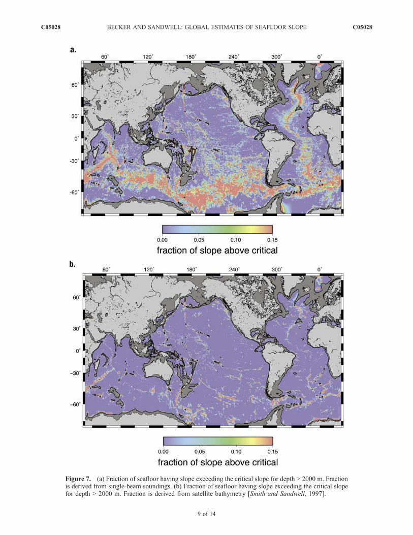
Figure 7. (a) Fraction of seafloor having slope exceeding the critical slope for depth > 2000 m. Fractionis derived from single-beam soundings. (b) Fraction of seafloor having slope exceeding the critical slopefor depth > 2000 m. Fraction is derived from satellite bathymetry [Smith and Sandwell, 1997].


9 of 14

C05028

Sandwell [1997] grid was calculated, we would expectslopes from the gradient of Smith and Sandwell [1997] tobe p/2 times greater than single-beam slopes, and thus thefraction of seafloor above the critical slope should be p/2larger. Instead, we find the supercritical fraction of seafloorfor [Smith and Sandwell, 1997] to be substantially less thanthat derived from the single-beam soundings. This is be-cause, as discussed above, satellite bathymetry does notcapture the full magnitude of the seafloor gradient because itonly resolves wavelengths > 20 km.[25] The ship data and the satellite bathymetry grid have

similar supercritical seafloor fraction for the large-scalestructures of the ocean basins such as continental margins,ridge axes, ocean trenches and back-arc volcanoes andintraplate island chains such as Hawaii. This is expectedbecause these large-scale features are well resolved in thesatellite bathymetry grid. However, there are major differ-ences (Figures 7a and 7b) on the flanks of ridges especiallyin the Southern Ocean where the critical slope at the bottomof the ocean is less than 0.2 m/m.[26] To quantify this observation we plot the area of

seafloor with supercritical slope versus ocean depth(Figure 8, thick line). Seafloor spreading ridges lie at depthsbetween 2000 m and 3000 m. The ridge flanks lie at depthsbetween 3000 m and 4500 m. It is clear that the fraction ofsupercritical seafloor on the ridge flanks is larger than thefraction of supercritical seafloor on the ridge axes. A similaranalysis using satellite bathymetry arrives at just the oppo-site conclusion and suggests that the ridge axes are moreimportant than the ridge flanks. Indeed the total fraction ofsupercritical seafloor in the deep ocean (>2000 m deep) is4.5% based on the single-beam data and only 1.5% basedon the satellite bathymetry. These comparisons suggests thatcalculations based on slopes of the [Smith and Sandwell,

1997] grid are substantially underestimating the area ofsuper critical seafloor, and its location.

8. Discussion and Conclusions

[27] We restrict our discussion to the deeper ocean areas(>2000 m) where abyssal hills dominate the seafloor slope,and where we expect that spatial variations in slope andcritical slope will be smooth relative to the characteristicspacing of the ship profiles. Our estimate of the fraction ofseafloor above critical slope shows some obvious globalpatterns that deserve comment. The west flank of thesouthern Mid-Atlantic Ridge is prominent, but areas ofrough seafloor in the Southern Ocean dominate the fractionof seafloor above critical. In particular, the flanks of theSouthwest Indian Ridge and the flanks of the SoutheastIndian Ridge, especially in the Australian-Antarctic Discor-dant Zone (90�E�160�E) are prominent as are the flanks ofthe Pacific-Antarctic Rise, and the flanks of the Scotia SeaSpreading Centers (50�S�60�S, 75�W�30�W). The pres-ence of so much super critical topography near the AntarcticCircumpolar Current (ACC) is striking. We speculate thatthe ACC may be sweeping the sediment off the ridge flanks,creating an area of rough topography in a strong current.[28] Our conclusions are as follows.[29] 1. The 40-year archive of single-beam bathymetry

provides a global perspective on the slope and roughness ofthe seafloor although the data have some significant short-comings. First, the original data are highly heterogeneousbecause they were collected with multiple generations ofecho sounding and navigation technology and were digi-tized and assembled by hundreds of scientists on tens ofresearch vessels. By visually editing 4900 cruises assembledat NGDC, we were able to extract seafloor slope and

Figure 8. Area of seafloor with above critical slope as a function of depth. Thick curve is from single-beam data while the thin curve is from satellite bathymetry. Seafloor slopes from satellite bathymetryclearly underestimate supercritical area with depth < 2000 m. The critical slope calculation is unreliablefor shallow depths < 2000 m.


10 of 14

C05028

roughness information for wavelengths greater than 2 kmand confirmed the results in small areas where completemultibeam coverage is available. A second problem with thesingle-beam bathymetry data is that the seafloor slope canonly be estimated along the trackline of the ship, which isusually not in the direction of maximum seafloor gradient.Assuming the direction of the ship tracks is random withrespect to the abyssal hill fabric, we show that, on average,the along-track slope will be 2/p less than the magnitude ofthe gradient. We use the along-track slope estimate as aproxy for seafloor slope knowing it represents a lowerbound on the actual slope.[30] 2. The critical slope at the bottom of the ocean

associated with conversion of the barotropic M2 tide wasestimated from a global compilation of temperature andsalinity measurements [Conkright et al., 2007]. Sparsemeasurements, especially in the Southern Ocean, preventthe construction of a spatially detailed map of critical slope.We argue that in the deep ocean (<2000 m) spatial varia-tions in temperature and salinity will be small so this globalrepresentation may be qualitatively correct. Interpolatingthis critical slope map to the locations of the measuredseafloor slope, we estimate the fraction of seafloor withslope that exceeds the critical value. In contrast to previousstudies based on altimetry-derived depth, we find largeareas that have slope exceeding the critical value.[31] 3. Our results are consistent with previous studies

that show a high fraction of seafloor above critical slopealong the Mid-Atlantic Ridge and Hawaiian Chain butsuggest that barotropic tidal conversion dominantly occursin the Southern Ocean where sediments are thin and theabyssal hills have relatively high amplitude because theyformed at a fossil spreading rate less than the thresholdvalue of 70 mm/a. The global analysis shows that the largestareas of supercritical slope are on the flanks of the seafloorspreading ridges. The largest areas of supercritical slope arethe Southwest Indian Ridge flanks, the Southeast IndianRidge flanks, the southern Mid-Atlantic Ridge flanks, theScotia Ridge, and most importantly, the Pacific AntarcticRise away from the ridge axis.

Appendix A: Comparison of Critical Slope FromWOCE P16 CTD Casts and Numerical Fits toWOA 2001

[32] The global map of critical slope (Figure 1) showsobvious hemispherical variation with the lower critical slopein the South Pacific than North Pacific. To verify thishemispherical asymmetry, we compared our numerical fitof World Ocean Atlas (WOA) 2001 data [Conkright et al.,2007] to the critical slope calculated from Salinity, Temper-ature, and Pressure data (commonly referred to as CTD) fromtwo World Ocean Circulation Experiment (WOCE) repeatcruises in 2005/2006. These cruises revisited the ‘‘P16’’ linein the Pacific that runs along longitude 150�W from Antarc-tica to Alaska with a CTD cast taken at least once everydegree of latitude from 72�S to 56�N. These particular datawere not used in the WOA 2001 analysis [Conkright et al.,2007]. The 2005/2006 cruises had modern navigation andCTD instrumentation and they sampled the entire watercolumn from surface to approximately 10m above the bot-tom. A typical CTD rosette has redundant sensors that are

calibrated on shore and against each other on each station.The noise present in the data is on the order of 1 part perthousand or better. This level of instrument noise is inconse-quential since the microstructure of the water column dom-inates the instrumentation noise. The standard deviation of Ndue to the microstructure was typically 0.25 cph in thedeepest bin, which is a large fraction of the total estimate ofN so this environmental noise dominates. At one station in theNorth Pacific at 28�N, either an overturn was observed at thebottom, or there was a data error large enough to create anegative N2. As in the cases of computing N from the WOA,this value of N and the critical slope are both set to zero.[33] The CTD data from 190 casts were processed into

critical slope at the bottom of the ocean as follows. The‘‘exchange’’ data in comma separated value (CSV) formatfrom the 2005 repeat of the P16S line on cruise33RR200501, and the 2006 repeat of P16N from cruise325020060213 were down loaded from the CLIVAR &Carbon Hydrography Office (CCHDO) website (J. Swift,http://cchdo.ucsd.edu, accessed 2 January 2008) and pro-cessed using MATLAB software [MathWorks, 2007]. Foreach of the depth casts, the CTD were processed using theCSIRO algorithm [Morgan and Pender, 2003] of theUNESCO seawater equation of state. The data for each castwere then binned and averaged at the WOA standarddepths. The deepest bin in each P16 station was comparedto the numerical fit from the WOA 2001 data [Conkright etal., 2007]. The maximum depth of the water at P16 stationsis rarely more than 100 m deeper than the maximumstandard depth in the WOA.[34] Estimates of critical slope from the WOA and P16

are plotted in Figure A1 and show good agreement. Bothestimates have an unknown uncertainty that is dominated bytrue fluctuations in density gradient. Therefore we per-formed a robust regression [Laws, 1997] using a ‘‘bisquare’’weighting function in the MATLAB robustfit functionwhere the model was constrained to go through the origin.Our calculation of critical slope using the WOA is slightlysmaller than the experimental data (0.958 ± 0.085), but it iswithin 5 percent of the experimental result and is consistentwith a slope of one. The linear correlation is 0.497. TheWOA data also show some anomalously high slopes thatare due to underestimating the density gradient. Consideringthat the microstructure of N in the experimental data isapproximately ±50%, we feel our use of a fit to the WOA toestimate global critical slope is justified.[35] Given this level of agreement we believe the north-

south asymmetry in critical slope, shown in Figure 1, is real.Along this line of longitude the asymmetry is to be expectedbecause of the Pacific basin in the northern hemisphere isgenerally 1–2 km deeper than the flank of the PacificAntarctic Rise in the southern hemisphere and deeper oceantends to be more stratified than shallower ocean. In conclu-sion, a critical slope calculated from WOA is error prone,but in good agreement with the more accurate CTD data.

Appendix B: Statistical Relationship BetweenSlope and Gradient

[36] Assume the abyssal seafloor away from isolatedseamounts and other distinct features is a stationary andergodic function [Bendat and Piersol, 2000]. The gradient


11 of 14

C05028

of a randomly oriented facet of seafloor is a random vector[Goff, 1991]. Our objective is to describe the statisticalproperties of the gradient vector as well as to relate this tothe statistical properties of the slope vector. Following Goff[1991], assume the x- and y-components of the gradient areindependent, zero mean, and normally distributed with

identical variance s2. As discussed by Freilich [1997], thehistogram of the magnitude of this random vector is aRayleigh distribution (x > 0)

fRayleigh x;sð Þ ¼ x

s2exp

�x2

2s2

� �: ðB1Þ

Figure A1. (a) Scatterplot of critical slope calculated from WOA and P16 cruise data. (b) Meridionalplot of critical slope calculated from WOA and P16 cruise data.


12 of 14

C05028

[37] The mean value of the gradient g is

�g ¼Z1

g¼0

g f g; sð Þdg ¼ sffiffiffip2

r: ðB2Þ

[38] Given this statistical model for seafloor slope we canrelate the probability distribution of along-track slope to theRayleigh distribution of gradient. Consider a tilted facet ofseafloor oriented at an azimuth of f with respect to the trackline of the ship. The measured slope of the seafloor isalways less than or equal to the magnitude of the gradientand it is given by s = gcosf. The distribution for along trackslope is related to the probability distribution for gradient by

f s;f;sð Þ ¼ fRayleigh s= cosf;sð Þ @g@s

��

¼ s

s2 cos2 fexp

�s2

2s2 cos2 f

� �: ðB3Þ

[39] We need to integrate over all azimuths and normalizeby 2p to obtain the distribution for a randomly oriented facet.

f s; sð Þ ¼ 1

2p

Z2p

0

f s;f; sð Þdf ¼ffiffiffiffiffiffiffiffi2

ps2

rexp

�s2

2s2

� �: ðB4Þ

[40] The Rayleigh distribution describing the gradientmaps to a Gaussian distribution describing the along track

slope. An example of theoretical gradient and slopedistribution functions are shown in Figure B1 along withthe histograms of observed gradient and slope shown inFigure 5. While there are discrepancies between the actualand model distribution functions, these simple ideas providean approximate basis for deriving seafloor gradient infor-mation from along-track slope profiles. In particular, it isinteresting to relate the mean along track slope to the meangradient, (s > 0)

�s ¼Z1

0

s f s;sð Þds ¼ s

ffiffiffi2

p

r¼ 2

p�g: ðB5Þ

[41] This relationship suggests the mean value of slopemeasured along a ship track is lower than the gradient by afactor of 2/p (64%). In this paper, we compute mean slopealong ship tracks, and expect that the seafloor gradient isusually larger.

[42] Acknowledgments. This paper benefited greatly from discus-sions with Walter Munk, Stefan Llewellyn Smith, Shaun Johnston, SarahGille, and Jennifer MacKinnon. Scott Nelson of UCSD edited the ship datawith an astonishing rapidity and accuracy. We thank the Associate EditorJames Richman and the two reviewers for their many suggestions forimproving the manuscript. We also thank Walter Munk for originallyproposing this study in 1999 using satellite bathymetry. That preliminarycomparison suggested (incorrectly) that the abyssal plains were not impor-tant in deep ocean mixing. The results were not published because wespeculated that the slope of the seafloor from satellite bathymetry greatlyunderestimates the true seafloor slope. It has taken 8 years to go back, look

Figure B1. Histograms of the magnitude of the slope (blue) and gradient (red) for the data shown inFigure 5. The theoretical histogram for a Rayleigh distribution with a mean slope of 0.152 m/m providesan adequate fit to the actual gradient distribution. Mapping the gradient distribution into slope distributionprovides an adequate fit to the actual slope distribution. The mean value of the theoretical slopedistribution is 2/p times the mean value of the gradient distribution.


13 of 14

C05028

at the raw sounding data, and arrive at a more accurate assessment. Thisresearch was supported by the Office of Naval Research (N00014-06-1-0140) and the National Science Foundation (OCE-0326707).

ReferencesBaines, P. G. (1982), On internal tide generation models, Deep Sea Res.,Part I, 29, 307–338, doi:10.1016/0198-0149 (82)90098-X.

Bendat, J. S., and A. G. Piersol (2000), Measurement and Analysis ofRandom Data, 3rd ed., John Wiley, Hoboken, N.J.

Cannat, M., D. Sauter, V. Mendel, E. Ruellan, K. Okino, J. Escartin,V. Combier, and M. Baala (2006), Modes of seafloor generation at a melt-poor ultraslow-spreading ridge, Geology, 34(7), 605–608, doi:10.1130/G22486.1.

Canuto, V. M., A. Howard, Y. Cheng, and R. L. Miller (2004), Latitude-dependent vertical mixing and the tropical thermocline in a globalOGCM, Geophys. Res. Lett., 31, L16305, doi:10.1029/2004GL019891.

Carbotte, S. M., et al. (2004), New integrated data management system forRidge2000 and MARGINS research, Eos Trans. AGU, 85(51),553,doi:10.1029/2004EO510002.

Conkright, M. E., et al. (2007), World Ocean Atlas 2001, http://www.nodc.noaa.gov/OC5/WOA01/pr_woa01.html, Natl. Oceanogr. Data Cent.,Silver Spring, Md., 2 Jan.

Dillon, T. M. (1982), Vertical overturns: A comparison of Thorpe andOzmidov length scales, J. Geophys. Res., 87(C12), 9601 – 9613,doi:10.1029/JC087iC12p09601.

Egbert, G. D., and R. D. Ray (2000), Significant dissipation of tidal energyin the deep ocean inferred from satellite altimeter data, Nature,405(6788), 775–778, doi:10.1038/35015531.

Egbert, G. D., and R. D. Ray (2001), Estimates of M2 tidal energy dissipa-tion from TOPEX/POSEIDON altimeter data, J. Geophys. Res.,106(C10), 22,475–22,502, doi:10.1029/2000JC000699.

Egbert, G. D., and R. D. Ray (2003), Semi-diurnal and diurnal tidal dis-sipation from TOPEX/POSEIDON altimetry, Geophys. Res. Lett., 30(17),1907, doi:10.1029/2003GL017676.

Freilich, M. H. (1997), Validation of vector magnitude datasets: Effects ofrandom component errors, J. Atmos. Oceanic Technol., 14(3), 695–703,doi:10.1175/1520-0426 (1997)014<0695:VOVMDE>2.0.CO;2.

Garrett, C., and E. Kunze (2007), Internal tide generation in the deepocean, Annu. Rev. Fluid Mech., 39, 57 – 87, doi:10.1146/annurev.fluid.39.050905.110227.

Gille, S. T., M. M. Yale, and D. T. Sandwell (2000), Global correlation ofmesoscale ocean variability with seafloor roughness from satellite altime-try, Geophys. Res. Lett., 27(9), 1251–1254, doi:10.1029/1999GL007003.

Goff, J. A. (1991), A global and regional stochastic analysis of near-ridgeabyssal hill morphology, J. Geophys. Res., 96(B13), 21,713–21,737,doi:10.1029/91JB02275.

Goff, J. A., and T. H. Jordan (1989), Stochastic modeling of seafloormorphology: A parameterized Gaussian model, Geophys. Res. Lett.,16(1), 45–48, doi:10.1029/GL016i001p00045.

Goff, J. A., and W. H. F. Smith (2003), A correspondence of altimetricgravity texture to abyssal hill morphology along the flanks of the South-east Indian Ridge, Geophys. Res. Lett., 30(24), 2269, doi:10.1029/2003GL018913.

Goff, J. A., W. H. F. Smith, and K. M. Marks (2004), The contributionsof abyssal hill morphology and noise to altimetric gravity fabric,Oceanography, 17(1), 24–37.

Jayne, S. R., and L. C. St Laurent (2001), Parameterizing tidal dissipationover rough topography, Geophys. Res. Lett., 28(5), 811 – 814,doi:10.1029/2000GL012044.

Kantha, L. H. (1995), Barotropic tides in the global oceans from a nonlineartidal model assimilating altimetric tides: 1. Model description and results,J. Geophys. Res., 100(C12), 25,283–25,308, doi:10.1029/95JC02578.

Knauss, J. A. (1997), Introduction to Physical Oceanography, 2nd ed.,309 pp., Prentice Hall, Upper Saddle River, N. J.

Kunze, E., and S. G. Llewellyn Smith (2004), The role of small-scaletopography in turbulent mixing of the global ocean, Oceanography,17(1), 55–64.

Laws, E. (1997), Mathematical Methods for Oceanographers: An Introduc-tion, 343 pp., John Wiley, Hoboken, N. J.

Ledwell, J. R., E. T. Montgomery, K. L. Polzin, L. C. St. Laurent, R. W.Schmitt, and J. M. Toole (2000), Evidence for enhanced mixing over

rough topography in the abyssal ocean, Nature, 403(6766), 179–182,doi:10.1038/35003164.

Llewellyn Smith, S. G., and W. R. Young (2002), Conversion of the bar-otropic tide, J. Phys. Oceanogr., 32(5), 1554–1566, doi:10.1175/1520-0485(2002)032<1554:COTBT>2.0.CO;2.

Lonsdale, P. (1977), Deep-tow observations at Mounds Abyssal Hydrother-mal Field, Galapagos Rift, Earth Planet. Sci. Lett., 36(1), 92–110,doi:10.1016/0012-821X(77)90191-1.

Macdonald, K. C. (1982),Mid-ocean ridges: Fine scale tectonic, volcanic andhydrothermal processes within the plate boundary zone, Annu. Rev. EarthPlanet. Sci., 10, 155–190, doi:10.1146/annurev.ea.10.050182.001103.

Macdonald, K. C., and B. P. Luyendyk (1985), Investigation of faulting andabyssal hill formation on the flanks of the East Pacific Rise (21�N) usingAlvin, Mar. Geophys. Res., 7(4), 515–535, doi:10.1007/BF00368953.

Macdonald, K. C., P. J. Fox, L. J. Perram, M. F. Eisen, R. M. Haymon, S. P.Miller, S. M. Carbotte, M.-H. Cormier, and A. N. Shor (1988), A newview of the mid-ocean ridge from the behavior of ridge-axis discontinu-ities, Nature, 335(6187), 217–225, doi:10.1038/335217a0.

Macdonald, K. C., P. J. Fox, R. T. Alexander, R. Pockalny, and P. Gente(1996), Volcanic growth faults and the origin of Pacific abyssal hills,Nature, 380(6570), 125–129, doi:10.1038/380125a0.

MathWorks (2007), MATLAB, software, Natick, Mass.Menard, H. W. (1967), Sea floor spreading topography and second layer,Science, 157(3791), 923–924, doi:10.1126/science.157.3791.923.

Morgan, P., and L. Pender (2003), SEAWATER: A library of MATLABcomputational routines for the properties of seawater, report, CSIRO Div.of Mar. Res., Melbourne, Victoria, Australia.

Munk, W. (1966), Abyssal recipes, Deep Sea Res. Part I, 13, 707–730.Munk, W., and C. Wunsch (1998), Abyssal recipes II: Energetics of tidaland wind mixing, Deep Sea Res., Part I, 45, 1977–2010, doi:10.1016/S0967-0637 (98)00070-3.

Nash, J. D., M. H. Alford, E. Kunze, K. Martini, and S. Kelly (2007),Hotspots of deep ocean mixing on the Oregon continental slope,Geophys. Res. Lett., 34, L01605, doi:10.1029/2006GL028170.

National Geophysical Data Center (2006), GEODAS search criteria selec-tion, http://ftp.ngdc.noaa.gov/mgg/gdas/gd_cri.Html, Boulder, Colo.,2 Jan.

Osborn, T. R. (1980), Estimates of the local-rate of vertical diffusion fromdissipation measurements, J. Phys. Oceanogr., 10(1), 83–89, doi:10.1175/1520-0485(1980)010<0083:EOTLRO>2.0.CO;2.

Osborn, T. R., and C. S. Cox (1972), Oceanic fine structure, Geophys. FluidDyn., 3, 321–345, doi:10.1080/03091927208236085.

Polzin, K. L., J. M. Toole, J. R. Ledwell, and R. W. Schmitt (1997), Spatialvariability of turbulent mixing in the abyssal ocean, Science, 276(5309),93–96, doi:10.1126/science.276.5309.93.

Small, C., and D. T. Sandwell (1992), An analysis of ridge axis gravityroughness and spreading rate, J. Geophys. Res., 97(B3), 3235–3245,doi:10.1029/91JB02465.

Smith, W. H. F. (1993), On the accuracy of digital bathymetric data,J. Geophys. Res., 98(B6), 9591–9603, doi:10.1029/93JB00716.

Smith, W. H. F. (1998), Seafloor tectonic fabric from satellite altimetry,Annu. Rev. Earth Planet. Sci., 26, 697 –747, doi:10.1146/annurev.earth.26.1.697.

Smith, W. H. F., and D. T. Sandwell (1997), Global sea floor topographyfrom satellite altimetry and ship depth soundings, Science, 277(5334),1956–1962, doi:10.1126/science.277.5334.1956.

Smith, W. H. F., and D. T. Sandwell (2004), Conventional bathymetry,bathymetry from space, and geodetic altimetry, Oceanography, 17(1),8–23.

St. Laurent, L., and C. Garrett (2002), The role of internal tides in mixingthe deep ocean, J. Phys. Oceanogr., 32(10), 2882–2899, doi:10.1175/1520-0485(2002)032<2882:TROITI>2.0.CO;2.

Toole, J. M., R. W. Schmitt, K. L. Polzin, and E. Kunze (1997), Near-boundary mixing above the flanks of a midlatitude seamount, J. Geophys.Res., 102(C1), 947–959, doi:10.1029/96JC03160.

Wessel, P., and W. H. F. Smith (1995), New version of the generic mappingtools released, Eos Trans. AGU, 79(47), 579, doi:10.1029/95EO00216.

��J. J. Becker and D. T. Sandwell, Institute of Geophysics and Planetary

Physics, Scripps Institution of Oceanography, 8795 Biological Grade,Room 1102, La Jolla, CA 92037, USA. ([email protected])


14 of 14

C05028

global estimates of seafloor slope from single-beam ship...

Documents