mathematics

Article

Global Dynamics of an SIQR Model with Vaccinationand Elimination Hybrid Strategies

Yanli Ma 1, Jia-Bao Liu 2,* and Haixia Li 1

1 Department of General Education, Anhui Xinhua University, Hefei 230088, China;Linda-mayanli@163.com (Y.M.); learain1@126.com (H.L.)

2 School of Mathematics and Physics, Anhui Jianzhu University, Hefei 230601, China* Correspondence: liujiabaoad@163.com or liujiabao@ahjzu.edu.cn

Received: 18 October 2018; Accepted: 6 December 2018; Published: 14 December 2018�����������������

Abstract: In this paper, an SIQR (Susceptible, Infected, Quarantined, Recovered) epidemic modelwith vaccination, elimination, and quarantine hybrid strategies is proposed, and the dynamics ofthis model are analyzed by both theoretical and numerical means. Firstly, the basic reproductionnumber R0, which determines whether the disease is extinct or not, is derived. Secondly, by LaSallesinvariance principle, it is proved that the disease-free equilibrium is globally asymptotically stablewhen R0 < 1, and the disease dies out. By Routh-Hurwitz criterion theory, we also prove that thedisease-free equilibrium is unstable and the unique endemic equilibrium is locally asymptoticallystable when R0 > 1. Thirdly, by constructing a suitable Lyapunov function, we obtain that theunique endemic equilibrium is globally asymptotically stable and the disease persists at this endemicequilibrium if it initially exists when R0 > 1. Finally, some numerical simulations are presented toillustrate the analysis results.

Keywords: basic reproductive number; equilibrium; stability; SIQR epidemic model; vaccination;elimination

1. Introduction

As we know, infectious diseases cause the loss of billions of lives and bring great pain to millions offamilies. The whole world has devoted efforts to avoid the outbreak of the disease. Mathematical modelshave become important tools in analyzing the spread and control of infectious diseases. Almost 250 yearsago, Bernoulli presented some works on human epidemiology with the help of mathematical models.Toward the beginning of the 2nd quarter of the 20th century, Kermack and McKendric [1] establishedthe classical SIR model on epidemiology. Later on, many mathematical models had been proposed forthe transmission dynamics of infectious diseases [2–9]. In recent years, some works have been studiedfor mathematical analysis of human diseases and epidemic models also utilising dynamical systemapproaches as stability analysis, LaSalle’s invariance principle, Routh-Hurwitz criterion, or Lyapunovfunction in combination with numerical studies [10–14]. These models provided theoretical andquantitative bases for the prevention and control of infectious diseases.

Quarantine is the most direct control strategy for the spread of infectious disease. It has been usedto reduce the transmission of human diseases such as leprosy, plague, cholera, typhus, yellow fever,smallpox, diphtheria, tuberculosis 25, and measles etc, and also been used to tackle animal diseasessuch as rinderpest, foot and mouth disease, psittacosis, asian fowl plague, and rabies etc. Hence, it isvery important to study the infectious disease models with quarantine [15–18]. Vaccination isconsidered to be the most effective intervention strategy. It has been used to tackle diseases suchas measles, mumps, rubella, diphtheria, tetanus, influenza, polio, etc. Recently, the epidemiologicalmodels with vaccination strategy have been analyzed by many authors in [19–27]. For example,

Mathematics 2018, 6, 328; doi:10.3390/math6120328 www.mdpi.com/journal/mathematics

Mathematics 2018, 6, 328 2 of 12

Li et al. [19] discussed the global analysis of SIS epidemic model with a simple vaccination andmultiple endemic equilibria; Liu et al. [20] established two SVIR models by considering the timefor them to obtain immunity and the possibility for them to be infected before this; Trawicki [21]proposes a new SEIRS model with vital dynamics (birth and death rates), vaccination, and temporaryimmunity provides a mathematical description of infectious diseases and corresponding spread inbiology; T.K. Kar et al. [23] focused on the study of a nonlinear mathematical SIR epidemic modelwith a vaccination program, and the results showed that an accurate estimation of the efficiency ofvaccination is necessary to prevent and control the spread of disease. We also refer the readers to [26,27]for relative studies on this respect. Elimination is also an effective measure to eliminate the sourceof infection, it is that the infected individuals were killed when they are found. It has been used totackle diseases caused by animals or spreading in animals such as avian in uenza, tuberculosis, tetanus,rotavirus infection, etc. However, these models only consider a single prevention and control strategy,there is scarce research on the hybrid case of these strategies.

Our objective of this paper is to consider an SIQR model with vaccination, elimination, andquarantine hybrid strategies. The rest of the paper is organized as follows. In Section 3, we formulate anSIQR model with vaccination, elimination and quarantine hybrid strategies. In Section 4, we determinethe basic reproduction number R0 and obtain the existence of equilibriums. In Section 5, we discussand analyze the local stability and the global stability of the equilibriums by Routh-Hurwitz criteriontheory and constructing suitable Lyapunov functions. In Section 6, we carry out numerical simulationsto illustrate the theoretical results. In Section 7, we present some discussions and illustrations aboutthe characteristics of different prevention and control strategies according to the expression of the basicreproductive number R0. In the last section, we give a conclusion and prospect for the research work.

2. Model Formulation

In this section, we formulate an SIQR model with vaccination, elimination, and quarantinehybrid strategies.

We assume that the total population is divided into four distinct epidemiological subclasses ofindividuals which are susceptible, infectious, quarantine, and recovered (removed) with sizes denotedby S(t), I(t), Q(t), and R(t), respectively. The total population size at time t is denoted by N(t),with N(t) = S(t) + I(t) + Q(t) + R(t). We establish the following SIQR epidemic model of ordinarydifferential equations

dSdt = Λ− βSI − µS− pS,dIdt = βSI − (µ + α1 + γ + q + δ)I,dQdt = δI − (ε + µ + α2)Q,dRdt = pS + γI + εQ− µR.

(1)

where Λ is the recruitment rate of the population, µ is the natural death rate of the population, α1 is thedisease-related death rate of the infective class, α2 is the disease-related death rate of the quarantineclass, β is the effective contact rate between the susceptible class and the infective class, γ is the naturalrecovery rate of the infective class, p is the vaccination rate of the susceptible class, δ is the quarantinerate of the infective class, ε is the removed rate from the quarantine class to the recovered class, q is theelimination rate of the infective class.

3. Equilibrium and Basic Reproductive Number

In this section, we determine the basic reproduction number R0 and obtain the existence of thedisease-free equilibrium E0 and the endemic equilibrium E∗ of system (1).

Summing up the four equations of system (1) and denoting

N(t) = S(t) + I(t) + Q(t) + R(t),

Mathematics 2018, 6, 328 3 of 12

havingN′(t) = Λ− µN − (α1 + q)I − α2Q ≤ Λ− µN.

By solving the formula of N′(t), we obtain

N(t) ≤ N(0)e−µt +Λµ(1− e−µt),

thuslim

t→+∞sup(N(t)) =

Λµ

.

From biological considerations, we study system (1) in the the following feasible region

D =

{(S, I, Q, R)|S ≥ 0, I ≥ 0, Q ≥ 0, R ≥ 0, S + I + Q + R ≤ Λ

µ

}.

Set the right sides of system (1) equal zero, that is,Λ− βSI − µS− pS = 0,

βSI − (µ + α1 + γ + q + δ)I = 0,

δI − (ε + µ + α2)Q = 0,

pS + γI + εQ− µR = 0.

(2)

We determine a disease-free equilibrium E0

(Λ

µ+p , 0, 0, Λp(µ+p)µ

)of system (1) using (2). Further,

if Λβ > (µ + p)(µ + α1 + γ + q + δ), we obtain an unique endemic equilibrium E∗(S∗, I∗, Q∗, R∗) ofsystem (1) using (2), where

S∗ =µ + α1 + γ + q + δ

β, I∗ =

µ + pβ

(Λ

µ + pβ

µ + α1 + γ + q + δ− 1)

,

Q∗ =δ

µ + α2 + ε

µ + pβ

(Λ

µ + pβ

µ + α1 + γ + q + δ− 1)

, R∗ =γI∗ + pS∗ + εQ∗

µ.

DefineR0 =

Λµ + p

β

µ + α1 + γ + q + δ.

The R0 is called the basic reproduction number of system (1). It is easy to obtain the following theorem.

Theorem 1. For system (1), there is always a disease-free equilibrium E0, and there is also an unique endemicequilibrium E∗ when R0 > 1.

4. Global Stability of Equilibriums

In this section, we study the global stability of the disease-free equilibrium E0

(Λ

µ+p , 0, 0, Λp(µ+p)µ

)and the endemic equilibrium E∗(S∗, I∗, Q∗, R∗) of system (1) by Routh-Hurwitz criterion theory andLaSalle’s invariance principle.

Theorem 2. If R0 < 1, the disease-free equilibrium E0 of system (1) is locally asymptotically stable. If R0 > 1,the disease-free equilibrium E0 is unstable.

Mathematics 2018, 6, 328 4 of 12

Proof. The Jacobian matrix of system (1) at the disease-free equilibrium E0 is

J(E0) =

−µ− p 0 0 0

0 β Λµ+p − (µ + α1 + γ + q + δ) 0 0

0 δ −µ− α2 − ε 0p γ ε −µ

.

The four eigenvalues of matrix J(E0) are

λ1 = −µ− p, λ2 =β

µ + α1 + γ + q + δ(R0 − 1), λ3 = −(µ + α2 + ε), λ4 = −µ.

Obviously, if R0 < 1, we have the relation λ2 < 0. Therefore, all eigenvalues of matrix J(E0) havenegative real parts. Hence, the disease-free equilibrium E0 is locally asymptotically stable. If R0 > 1,we get the relation λ2 > 0. Therefore, the matrix J(E0) has at least an eigenvalue with positive realpart. Thus, the disease-free equilibrium E0 is unstable. This completes the proof.

Theorem 3. If R0 < 1, the disease-free equilibrium E0 of system (1) is globally asymptotically stable.

Proof. Consider the following Lyapunov function

V(t) = I(t).

Calculating the derivative of V(t) along the positive solution of system (1), it follows that

dVdt

∣∣∣∣(1)

=dIdt

∣∣∣∣(1)

= βSI − (µ + α1 + γ + q + δ)I

= (βS− (µ + α1 + γ + q + δ)) I

≤(

βΛ

µ + p− (µ + α1 + γ + q + δ)

)= (µ + α1 + γ + q + δ)(R0 − 1)I

≤ 0.

Furthermore, V′ = 0 only if I = 0. The maximum invariant set in {(S, I, Q, R)|V′ = 0} is thesingleton {E0}. When R0 < 1, according to LaSalle’s invariance principle [28,29], it follows that

limt→+∞

I(t) = 0.

Then, we obtain the limit equations of system (1)dSdt = Λ− µS− pS,dQdt = −(ε + µ + α2)Q,dRdt = pS + εQ− µR.

So, the disease-free equilibrium E0 is globally attractive in the region D. Therefore, the disease-freeequilibrium E0 of system (1) is globally asymptotically stable when R0 < 1 combined with the localasymptotical stability of the disease-free equilibrium E0. Thus we complete the proof.

Theorem 4. If R0 > 1, the endemic equilibrium E∗ of system (1) is locally asymptotically stable.

Mathematics 2018, 6, 328 5 of 12

Proof. The Jacobian matrix of system (1) at the endemic equilibrium E∗ is

J(E∗) =

−µ− p− βI∗ −βS∗ 0 0

βS∗ β Λµ+p − (µ + α1 + γ + q + δ) 0 0

0 δ −µ− α2 − ε 0p γ ε −µ

.

The two eigenvalues of matrix J(E∗) are

λ3 = −(µ + α2 + ε), λ4 = −µ.

The other two eigenvalues are also the eigenvalues of following matrix

J∗(E∗) =

(−µ− p− βI∗ −βS∗

βS∗ β Λµ+p − (µ + α1 + γ + q + δ)

)

=

(R0 −βS∗

βS∗ (µ + α1 + γ + q + δ)(R0 − 1)

)Obviously, if R0 > 1, it follows that

tr(J∗(E∗)) = R0 + (µ + α1 + γ + q + δ)(R0 − 1) > 0,

det(J∗(E∗)) = R0(R0 − 1)(µ + α1 + γ + q + δ) + β2(S∗)2 > 0.

Therefore, all eigenvalues of matrix J(E∗) have negative real parts. According to Routh-Hurwitzcriterion, we obtain the endemic equilibrium E∗ of system (1) is locally asymptotically stable. Thus theproof is completed.

The global asymptotic stability of the endemic equilibrium is proved below.

Theorem 5. If R0 > 1, the endemic equilibrium E∗ of system (1) is globally asymptotically stable.

Proof. Since the front two equations of system (1) can be independent, we consider thefollowing subsystem {

dSdt = Λ− βSI − µS− pS,dIdt = βSI − (µ + α1 + γ + q + δ)I.

(3)

Consider the following Liapunov function

V(t) =12(S− S∗)2 + S∗

(I − I∗ − I∗ln

I∗

I

).

Calculating the derivative of V(t) along the positive solution of system (3), it follows that

dVdt

∣∣∣∣(3)

= (S− S∗)S′ + S∗(I − I∗)I′

I+ (Q−Q∗)Q′ + (R− R∗)R′

= −(µ + p)(S− S∗)2 − βI(S− S∗)2

≤ 0.

Mathematics 2018, 6, 328 6 of 12

Obviously, we can obtain that V(t) is positive definite and V′(t) is negative definite. Hence,the solution (S∗, I∗) of system (3) is globally asymptotically stable. When R0 > 1, any solutions ofsystem (3) converge to (S∗, I∗), equivalently, lim

t→+∞S(t) = S∗, lim

t→+∞I(t) = I∗.

Then prove: limt→+∞

Q(t) = Q∗, limt→+∞

R(t) = R∗.

Consider the third equation of system (1), we derive limit equation

dQdt

= δI∗ − (ε + µ + α2)Q. (4)

It is easy to show that Q∗ is the solution of Equation (4) and Q∗ is globally asymptoticallystable. According to the relation between limit system and original system, we therefore obtain thatlim

t→+∞Q(t) = Q∗. In the same way, we also obtain that lim

t→+∞R(t) = R∗.

Noting that if R0 > 1, the endemic equilibrium E∗ of system (1) is locally asymptotically stable,we conclude that if R0 > 1, the endemic equilibrium E∗ of system (1) is globally asymptotically stable.This completes the proof.

5. The Numerical Simulation

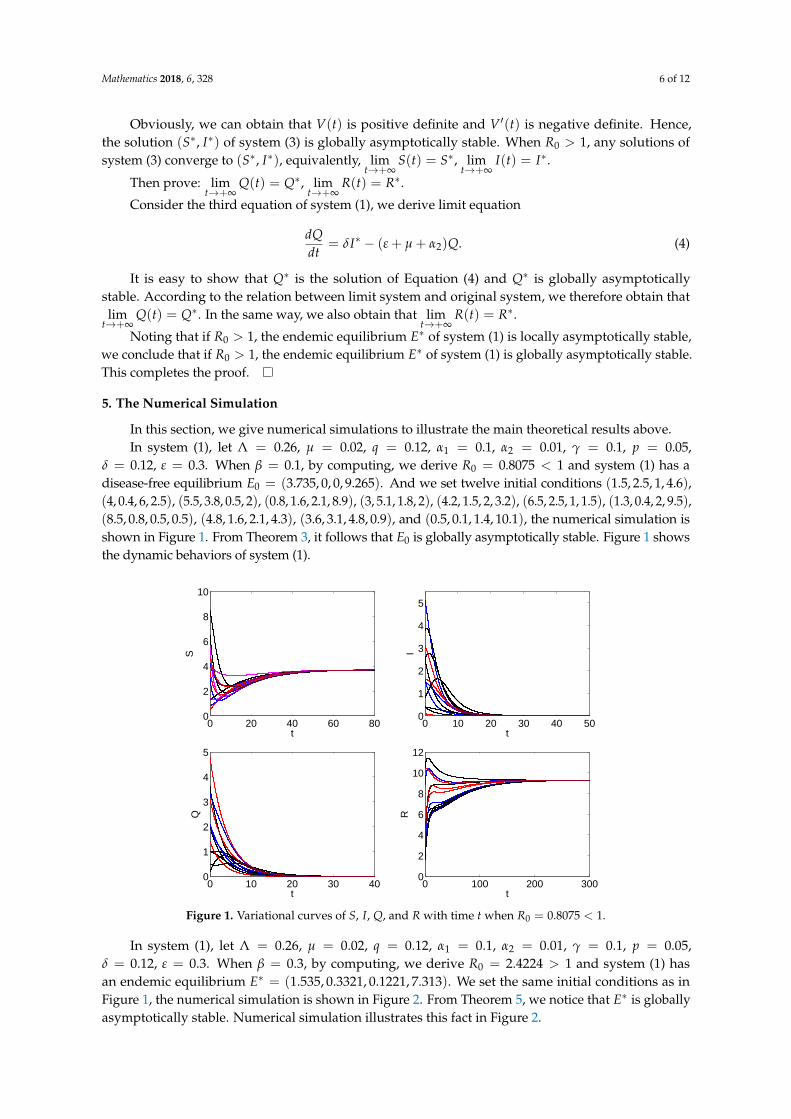
In this section, we give numerical simulations to illustrate the main theoretical results above.In system (1), let Λ = 0.26, µ = 0.02, q = 0.12, α1 = 0.1, α2 = 0.01, γ = 0.1, p = 0.05,

δ = 0.12, ε = 0.3. When β = 0.1, by computing, we derive R0 = 0.8075 < 1 and system (1) has adisease-free equilibrium E0 = (3.735, 0, 0, 9.265). And we set twelve initial conditions (1.5, 2.5, 1, 4.6),(4, 0.4, 6, 2.5), (5.5, 3.8, 0.5, 2), (0.8, 1.6, 2.1, 8.9), (3, 5.1, 1.8, 2), (4.2, 1.5, 2, 3.2), (6.5, 2.5, 1, 1.5), (1.3, 0.4, 2, 9.5),(8.5, 0.8, 0.5, 0.5), (4.8, 1.6, 2.1, 4.3), (3.6, 3.1, 4.8, 0.9), and (0.5, 0.1, 1.4, 10.1), the numerical simulation isshown in Figure 1. From Theorem 3, it follows that E0 is globally asymptotically stable. Figure 1 showsthe dynamic behaviors of system (1).

0 20 40 60 800

2

4

6

8

10

t

S

0 10 20 30 40 500

1

2

3

4

5

t

I

0 10 20 30 400

1

2

3

4

5

t

Q

0 100 200 3000

2

4

6

8

10

12

t

R

Figure 1. Variational curves of S, I, Q, and R with time t when R0 = 0.8075 < 1.

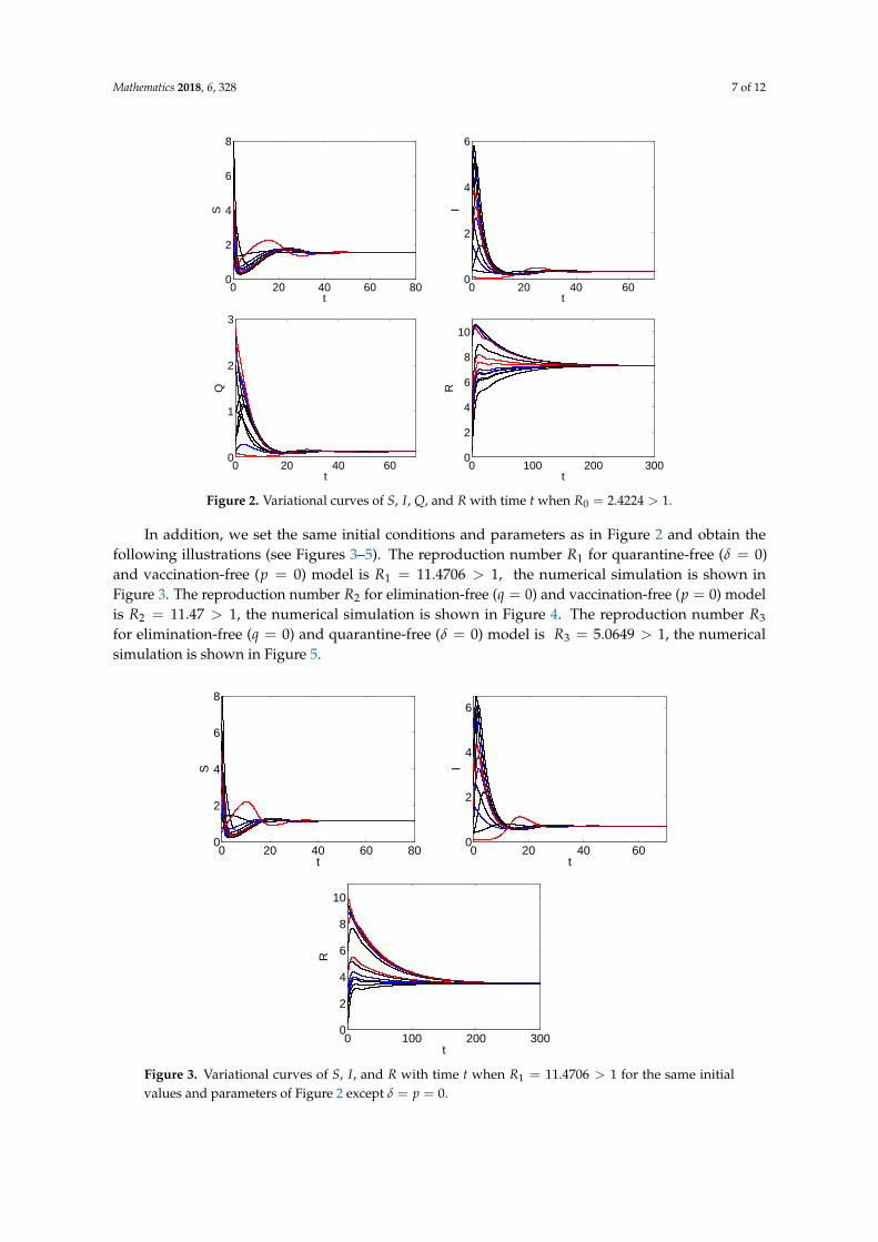
In system (1), let Λ = 0.26, µ = 0.02, q = 0.12, α1 = 0.1, α2 = 0.01, γ = 0.1, p = 0.05,δ = 0.12, ε = 0.3. When β = 0.3, by computing, we derive R0 = 2.4224 > 1 and system (1) hasan endemic equilibrium E∗ = (1.535, 0.3321, 0.1221, 7.313). We set the same initial conditions as inFigure 1, the numerical simulation is shown in Figure 2. From Theorem 5, we notice that E∗ is globallyasymptotically stable. Numerical simulation illustrates this fact in Figure 2.

Mathematics 2018, 6, 328 7 of 12

0 20 40 60 800

2

4

6

8

t

S

0 20 40 600

2

4

6

t

I0 20 40 60

0

1

2

3

t

Q

0 100 200 3000

2

4

6

8

10

t

R

Figure 2. Variational curves of S, I, Q, and R with time t when R0 = 2.4224 > 1.

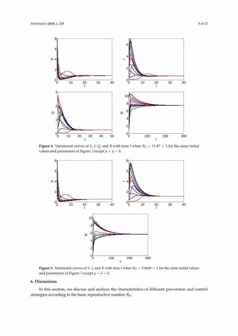
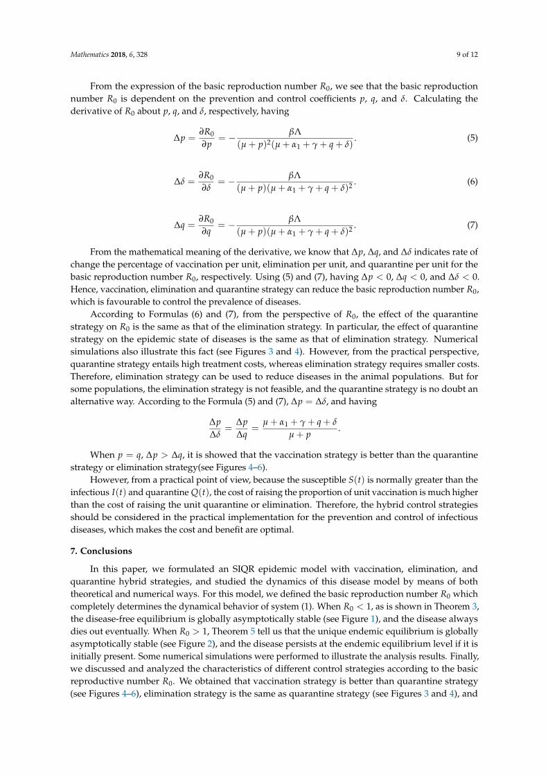
In addition, we set the same initial conditions and parameters as in Figure 2 and obtain thefollowing illustrations (see Figures 3–5). The reproduction number R1 for quarantine-free (δ = 0)and vaccination-free (p = 0) model is R1 = 11.4706 > 1, the numerical simulation is shown inFigure 3. The reproduction number R2 for elimination-free (q = 0) and vaccination-free (p = 0) modelis R2 = 11.47 > 1, the numerical simulation is shown in Figure 4. The reproduction number R3

for elimination-free (q = 0) and quarantine-free (δ = 0) model is R3 = 5.0649 > 1, the numericalsimulation is shown in Figure 5.

0 20 40 60 800

2

4

6

8

t

S

0 20 40 600

2

4

6

t

I

0 100 200 3000

2

4

6

8

10

t

R

Figure 3. Variational curves of S, I, and R with time t when R1 = 11.4706 > 1 for the same initialvalues and parameters of Figure 2 except δ = p = 0.

Mathematics 2018, 6, 328 8 of 12

0 10 20 30 400

2

4

6

8

t

S

0 10 20 30 400

2

4

6

t

I

0 10 20 30 40 500

1

2

3

t

Q

0 100 200 3000

2

4

6

8

10

t

R

Figure 4. Variational curves of S, I, Q, and R with time t when R2 = 11.47 > 1 for the same initialvalues and parameters of Figure 2 except p = q = 0.

0 10 20 30 400

2

4

6

8

t

S

0 10 20 30 400

2

4

6

8

t

I

0 100 200 3000

2

4

6

8

10

t

R

Figure 5. Variational curves of S, I, and R with time t when R3 = 5.0649 > 1 for the same initial valuesand parameters of Figure 2 except q = δ = 0.

6. Discussions

In this section, we discuss and analyze the characteristics of different prevention and controlstrategies according to the basic reproductive number R0.

Mathematics 2018, 6, 328 9 of 12

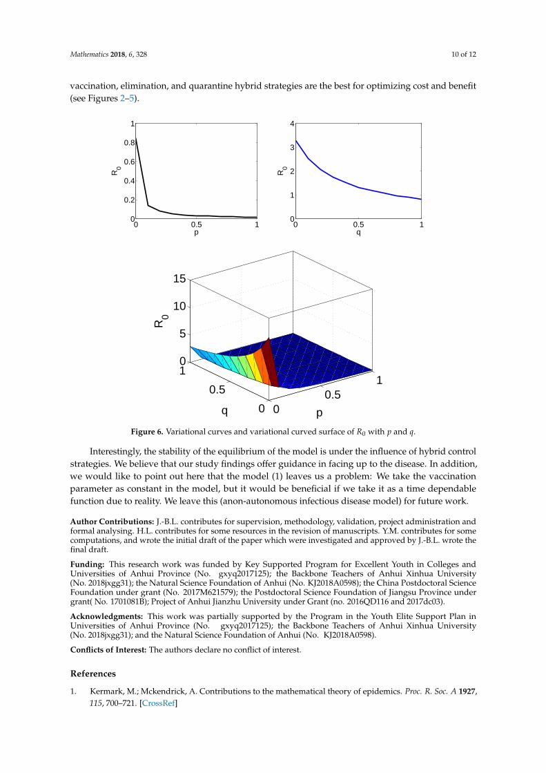
From the expression of the basic reproduction number R0, we see that the basic reproductionnumber R0 is dependent on the prevention and control coefficients p, q, and δ. Calculating thederivative of R0 about p, q, and δ, respectively, having

∆p =∂R0

∂p= − βΛ

(µ + p)2(µ + α1 + γ + q + δ). (5)

∆δ =∂R0

∂δ= − βΛ

(µ + p)(µ + α1 + γ + q + δ)2 . (6)

∆q =∂R0

∂q= − βΛ

(µ + p)(µ + α1 + γ + q + δ)2 . (7)

From the mathematical meaning of the derivative, we know that ∆p, ∆q, and ∆δ indicates rate ofchange the percentage of vaccination per unit, elimination per unit, and quarantine per unit for thebasic reproduction number R0, respectively. Using (5) and (7), having ∆p < 0, ∆q < 0, and ∆δ < 0.Hence, vaccination, elimination and quarantine strategy can reduce the basic reproduction number R0,which is favourable to control the prevalence of diseases.

According to Formulas (6) and (7), from the perspective of R0, the effect of the quarantinestrategy on R0 is the same as that of the elimination strategy. In particular, the effect of quarantinestrategy on the epidemic state of diseases is the same as that of elimination strategy. Numericalsimulations also illustrate this fact (see Figures 3 and 4). However, from the practical perspective,quarantine strategy entails high treatment costs, whereas elimination strategy requires smaller costs.Therefore, elimination strategy can be used to reduce diseases in the animal populations. But forsome populations, the elimination strategy is not feasible, and the quarantine strategy is no doubt analternative way. According to the Formula (5) and (7), ∆p = ∆δ, and having

∆p∆δ

=∆p∆q

=µ + α1 + γ + q + δ

µ + p.

When p = q, ∆p > ∆q, it is showed that the vaccination strategy is better than the quarantinestrategy or elimination strategy(see Figures 4–6).

However, from a practical point of view, because the susceptible S(t) is normally greater than theinfectious I(t) and quarantine Q(t), the cost of raising the proportion of unit vaccination is much higherthan the cost of raising the unit quarantine or elimination. Therefore, the hybrid control strategiesshould be considered in the practical implementation for the prevention and control of infectiousdiseases, which makes the cost and benefit are optimal.

7. Conclusions

In this paper, we formulated an SIQR epidemic model with vaccination, elimination, andquarantine hybrid strategies, and studied the dynamics of this disease model by means of boththeoretical and numerical ways. For this model, we defined the basic reproduction number R0 whichcompletely determines the dynamical behavior of system (1). When R0 < 1, as is shown in Theorem 3,the disease-free equilibrium is globally asymptotically stable (see Figure 1), and the disease alwaysdies out eventually. When R0 > 1, Theorem 5 tell us that the unique endemic equilibrium is globallyasymptotically stable (see Figure 2), and the disease persists at the endemic equilibrium level if it isinitially present. Some numerical simulations were performed to illustrate the analysis results. Finally,we discussed and analyzed the characteristics of different control strategies according to the basicreproductive number R0. We obtained that vaccination strategy is better than quarantine strategy(see Figures 4–6), elimination strategy is the same as quarantine strategy (see Figures 3 and 4), and

Mathematics 2018, 6, 328 10 of 12

vaccination, elimination, and quarantine hybrid strategies are the best for optimizing cost and benefit(see Figures 2–5).

0 0.5 10

0.2

0.4

0.6

0.8

1

p

R0

0 0.5 10

1

2

3

4

q

R0

00.5

1

0

0.5

10

5

10

15

pq

R0

Figure 6. Variational curves and variational curved surface of R0 with p and q.

Interestingly, the stability of the equilibrium of the model is under the influence of hybrid controlstrategies. We believe that our study findings offer guidance in facing up to the disease. In addition,we would like to point out here that the model (1) leaves us a problem: We take the vaccinationparameter as constant in the model, but it would be beneficial if we take it as a time dependablefunction due to reality. We leave this (anon-autonomous infectious disease model) for future work.

Author Contributions: J.-B.L. contributes for supervision, methodology, validation, project administration andformal analysing. H.L. contributes for some resources in the revision of manuscripts. Y.M. contributes for somecomputations, and wrote the initial draft of the paper which were investigated and approved by J.-B.L. wrote thefinal draft.

Funding: This research work was funded by Key Supported Program for Excellent Youth in Colleges andUniversities of Anhui Province (No. gxyq2017125); the Backbone Teachers of Anhui Xinhua University(No. 2018jxgg31); the Natural Science Foundation of Anhui (No. KJ2018A0598); the China Postdoctoral ScienceFoundation under grant (No. 2017M621579); the Postdoctoral Science Foundation of Jiangsu Province undergrant( No. 1701081B); Project of Anhui Jianzhu University under Grant (no. 2016QD116 and 2017dc03).

Acknowledgments: This work was partially supported by the Program in the Youth Elite Support Plan inUniversities of Anhui Province (No. gxyq2017125); the Backbone Teachers of Anhui Xinhua University(No. 2018jxgg31); and the Natural Science Foundation of Anhui (No. KJ2018A0598).

Conflicts of Interest: The authors declare no conflict of interest.

References

1. Kermark, M.; Mckendrick, A. Contributions to the mathematical theory of epidemics. Proc. R. Soc. A 1927,115, 700–721. [CrossRef]

Mathematics 2018, 6, 328 11 of 12

2. Misra, A.; Sharma, A.; Shukla, J. Stability analysis and optimal control of an epidemic model with awarenessprograms by media. Biosystems 2015, 138, 53–62. [CrossRef] [PubMed]

3. Ji, C.; Jiang, D.; Shi, N. The behavior of an SIR epidemic model with stochastic perturbation. Stoch. Anal. Appl.2012, 30, 755–773. [CrossRef]

4. Yang, Q.; Jiang, D.; Shi, N.; Ji, C. The ergodicity and extinction of stochastically perturbed SIR and SEIRepidemic models with saturated incidence. J. Math. Anal. Appl. 2012, 388, 248–271. [CrossRef]

5. Muroya, Y.; Enatsu, Y.; Nakata, Y. Global stability of a delayed SIRS epidemic model with a non-monotonicincidence rate. J. Math. Anal. Appl. 2011, 377, 1–14. [CrossRef]

6. Toshikazu, K.; Yoshiaki, M. Global stability of a multi-group SIS epidemic model with varying totalpopulation size. Appl. Math. Comput. 2015, 265, 785–798.

7. Muroya, Y.; Kuniya, T.; Wang, J. Stability analysis of a delayed multi-group SIS epidemic model withnonlinear incidence rates and patch structure. J. Math. Anal. Appl. 2015, 425, 415–439. [CrossRef]

8. Muroya, Y.; Li, H.; Kuniya, T. Complete global analysis of an SIRS epidemic model with graded cure andincomplete recovery rates. J. Math. Anal. Appl. 2014, 410, 719–732. [CrossRef]

9. Wang, W.J.; Xiao, Y.; Cheke, R.A. Modelling the effects of contaminated environments on HFMD infectionsin mainland China. Biosystems 2016, 140, 1–7. [CrossRef] [PubMed]

10. Elaiw, A.M.; Alade, S.M.; Alsulami, T.O. Global Stability of within-host Virus Dynamics Models withMultitarget Cells. Mathematics 2018, 6, 118. [CrossRef]

11. Tennenbaum, S.; Freitag, C.; Roudenko, S. Modeling the Influence of Environment and Intervention onCholera in Haiti. Mathematics 2014, 2, 136–171. [CrossRef]

12. Erhardt, A.H. Bifurcation Analysis of a Certain Hodgkin-Huxley Model Depending on Multiple BifurcationParameters. Mathematics 2018, 6, 103. [CrossRef]

13. Kuniya, T. Stability Analysis of an Age-Structured SIR Epidemic Model with a Reduction Method to ODEs.Mathematics 2018, 6, 147. [CrossRef]

14. Hategekimana, F.; Saha, S.; Chaturvedi, A. Dynamics of Amoebiasis Transmission: Stability and SensitivityAnalysis. Mathematics 2017, 5, 58. [CrossRef]

15. Mishra, B.K.; Jha, N. SEIQRS model for the transmission of malicious objects in computer network.Appl. Math. Model. 2010, 34, 710–715. [CrossRef]

16. Cesar, M.S. A nonautonomous epidemic model with general incidence and isolation. Math. Methods Appl. Sci.2014, 37, 1974–1991.

17. Yan, X.; Zou, Y. Optimal and sub-optimal quarantine and isolation control in SARS epidemics.Math. Comput. Model. 2008, 47, 235–245. [CrossRef]

18. Tan, X.X.; Li, S.J.; Dai, Q.W.; Gang, J.T. An epidemic model with isolated intervention based on cellularautomata. Adv. Mater. Res. 2014, 926, 1065–1068. [CrossRef]

19. Li, J.; Ma, Z.; Zhou, Y. Global analysis of SIS epidemic model with a simple vaccination and multiple endemicequilibria. Acta Math. Sci. 2006, 26, 83–93. [CrossRef]

20. Liu, X.; Takeuchi, Y.; Iwami, S. SVIR epidemic models with vaccination strategies. J. Theor. Biol. 2008, 253,1–11. [CrossRef] [PubMed]

21. Trawicki, M.B. Deterministic Seirs Epidemic Model for Modeling Vital Dynamics, Vaccinations, and TemporaryImmunity. Mathematics 2017, 5, 7. [CrossRef]

22. Chauhan, S.; Misra, O.P.; Dhar, J. Stability Analysis of SIR Model with Vaccination. Am. J. Comput. Appl. Math.2014, 4, 17–23.

23. Kar, T.; Batabyal, A. Stability analysis and optimal control of an SIR epidemic model with vaccination.Biosystems 2011, 104, 127–135. [CrossRef] [PubMed]

24. Liu, D.; Wang, B.; Guo, S. Stability analysis of a novel epidemics model with vaccination and nonlinearinfectious rate. Appl. Math. Comput. 2013, 221, 786–801. [CrossRef]

25. Lahrouz, A.; Omari, L.; Kiouach, D.; Belmaati, A. Complete global stability for an SIRS epidemic model withgeneralized non-linear incidence and vaccination. Appl. Math. Comput. 2012, 218, 6519–6525. [CrossRef]

26. Sun, C.; Yang, W. Global results for an SIRS model with vaccination and isolation. Nonlinear Anal. RealWorld Appl. 2010, 11, 4223–4237. [CrossRef]

27. Eckalbar, J.C.; Eckalbar, W.L. Dynamics of an SIR model with vaccination dependent on past prevalencewith high-order distributed delay. Biosystems 2015, 129, 50–65. [CrossRef]

Mathematics 2018, 6, 328 12 of 12

28. LaSalle, J.P. Stability theory of ordinary differential equations. J. Differ. Equ. 1968, 4, 57–65. [CrossRef]29. LaSalle, J.P. The Stability of Dynamical Systems; SIAM: Philadephia, PE, USA, 1976; p. 457.

c© 2018 by the authors. Licensee MDPI, Basel, Switzerland. This article is an open accessarticle distributed under the terms and conditions of the Creative Commons Attribution(CC BY) license (http://creativecommons.org/licenses/by/4.0/).