global assessment of trends in wetting and drying wetting ... · supplementary information: global...

Supplementary Information: Global assessment of trends inwetting and drying over land

Peter Greve1,2, Boris Orlowsky1, Brigitte Mueller1, Justin Sheffield3, Markus Reichstein4,Sonia I. Seneviratne1

1Institute for Atmospheric and Climate Science, ETH Zurich, Universitaetsstrasse 16, 8092 Zurich,Switzerland

2Center for Climate Systems Modeling (C2SM), ETH Zurich, Universitaetstrasse 16, 8092 Zurich,Switzerland

3Department of Civil and Environmental Engineering, Princeton University, Princeton, New Jersey 08544,USA

4Max Planck Institute for Biogeochemistry, 07745 Jena, Germany

July 23, 2014

1

Global assessment of trends in wetting and drying over land

SUPPLEMENTARY INFORMATIONDOI: 10.1038/NGEO2247

NATURE GEOSCIENCE | www.nature.com/naturegeoscience 1

© 2014 Macmillan Publishers Limited. All rights reserved.

http://dx.doi.org/10.1038/ngeo2247

A Data

Our validation relies on the Budyko framework, which relates E/P to Ep/P . Sections A.1, A.2and A.3 provide details of the investigated P , E and Ep datasets, respectively. The Budykoformulation by Fu (1981) contains the free parameter ω being related to climatological NDVI (Liet al., 2013), which we adjust according to NDVI data from the Global Inventory Modeling andMapping Studies (GIMMS) (Tucker et al., 2005). The P , E and Ep datasets are also used toanalyse dryness changes with respect to the land water balance (P vs. E) and the hydroclimaticregime (P vs. Ep).

A.1 Precipitation datasets

Table S1: P datasets in this study. All datasets cover the shorter validation period (1984 - 2005). Thedatasets which do not cover the longer period of the dryness change analysis (1948-05) are markedwith a star. We interpolated all datasets to a common regular 0.5◦ grid.

P Dataset Characteristics References

CRU interpolated gauge observations, no bias adjustment Harris et al. (2013)

GPCC interpolated gauge observations, no bias adjustment Rudolf et al. (2005)

GPCP* interpolated gauge observations combined with satellitedata, bias adj.

Adler et al. (2003)

UDel P interpolated gauge observations Legates and Willmott (1990a)

PREC/L interpolated gauge observations, no bias adjustment Chen et al. (2002)

CPC* interpolated gauge observations combined with satellitedata, no bias adj.

We use global monthly datasets of precipitation (P ) and evapotranspiration (E) to investigatechanges in the land water balance. All P datasets are based on observations, either interpolatedgauge observations only or combined with satellite measurements. All P datasets are listed inTable S1.

A.2 Evapotranspiration datasets

We use global monthly E datasets from various sources. Within the 1984-2005 validation periodthree observations-based ’diagnostic’ datasets are available. However, most other E datasetsare model-based, either driven by observations-based or reanalysis-based forcing. Notably, weuse data from the TRENDY project (Sitch et al., 2013) including six state of the art LSMs. All Edatasets are listed in Table S2. The subdivision of E datasets into different classes follows thenotation of Mueller et al. (2011).

A.3 Potential evaporation parameterization

Hydroclimatological regime shifts are found by analysing potential evaporation (Ep) in conjunc-tion with P . We use several methods of differing complexity to determine Ep from temperature

2


Table S2: E datasets in this study. All datasets cover the shorter validation period (1984 - 2005). Thedatasets which do not cover the longer period of the dryness change analysis (1948 - 2005) are indi-cated with a star. We interpolated all datasets to a common regular 0.5◦ grid. For detailed informationon the individual datasets the reader is referred to the given references. Further information on theTRENDY project is provided in Sitch et al. (2013)

.Variable/Class Dataset Characteristics Reference

Diagnostic MPI-BGC Statistical upscaling of flux observations Jung et al. (2010)

CSIRO* derived from the Budyko framework withobserved P and Penman-Monteith Ep

Leuning et al. (2008), Zhanget al. (2010)

GLEAM* Priestley and Taylor based algorithm basedon satellite observations only

Miralles et al. (2011)

LSMs VIC forced with improved NCEP reanalysis datafrom Sheffield et al. (2006)

Liang et al. (1994)

NOAH forced with improved NCEP reanalysis datafrom Sheffield et al. (2006)

Chen and Dudhia (2001), Eket al. (2003)

TRENDYLSMs

SDGVM Woodward and Lomas (1995)

CLM Oleson et al. (2010)

Orchidee-CN

forced CRU observations, Zaehle and Friend (2010), Za-ehle et al. (2011)

LPJ-GUESS merged with NCEP reanalysis data Smith et al. (2001)

TRIFFID TRENDY forcing, Sitch et al. (2013) Cox (2001)

HYLAND Levy et al. (2004)

Reanalysis ERA-Interim* no data-assimilation of observed precipita-tion

Dee et al. (2011)

NCEP-CFSR* data-assimilation of observed precipitation Saha et al. (2010)

MERRA* no data-assimilation of observed precipita-tion

Rienecker et al. (2011)

NCEP no data-assimilation of observed precipita-tion

Kanamitsu et al. (2002)

20CR no data-assimilation of observed precipita-tion, only assimilating surface air pressureand sea surface temperature

Compo et al. (2011)

3


Table S3: T and Rn datasets in this study. All datasets cover the shorter validation period (1984 -2005). The datasets which do not cover the longer period of the dryness change analysis (1948-05)are marked with a star. We interpolated all datasets to a common regular 0.5◦ grid.

.Variable Dataset Characteristics Reference

T

UDel (D) interpolated station data Legates and Willmott (1990b)

CRU (C) interpolated station data Harris et al. (2013)

Rn

SRB* (S) satellite derived Legates and Willmott (1990b)

ERA-I* (E-I) ERA-Interim reanalysis Dee et al. (2011)

NCEP (N) NCEP/NCAR reanalysis Kanamitsu et al. (2002)

20CR (2) 20th century reanalysis Compo et al. (2011)

and/or net radiation (see Table S3). The method of Priestley-Taylor (Priestley and Taylor, 1972)approximates Ep as

Ep =α

λ

(∆ · (Rn −G)

∆ + γ

), (1.1)

with λ being the latent heat of vaporization (λ = 2.45MJkg−1), γ the psychrometric constant(γ ≈ 0.054kPa/◦C for an average air pressure of 1013.25hPa) and G the ground heat flux (Gcould be neglected following Weiß and Menzel, 2008). The term ∆ is the slope of the saturationwater vapor pressure curve (depending on T only) and estimated by the Tetens-Murray equation(Murray, 1967). The term α = 1.26 is the Priestley-Taylor constant as suggested by Priestley andTaylor (1972). However, Maidment (1993) found that α = 1.26 is suitable for humid climates onlyand that α = 1.74 for arid climates avoids underestimation of Ep. We use here both approaches,denoted as PTc (constant α) and PT (adjusted α), as both approaches are widely used. ForPT, α is adjusted according to the Koeppen-Geiger climate classification. We use a classificationfrom Rubel and Kottek (2010), which is in very good agreement with Peel et al. (2007). Thisclassification uses α = 1.26 for tropical (group A), continental (group D) and humid mild temperateclimates ( Cfa, Cfb, Cfc, Cwa and Cwb), and α = 1.74 for dry (group B) as well as polar (group E)and arid mild temperate climates (Csa and Csb).

The Penman-Monteith method (Monteith, 1965) is the most sophisticated and widely used methodto determine Ep in LSMs. However, additional input variables other than T and Rn are requiredfor its computation (like e.g. wind speed, relative humidity and vegetation properties) and thus weuse a pre-compiled dataset (Sheffield et al., 2012).Rn essentially controls Ep and we are thus able to estimate Ep directly from Rn using λ by

Ep =Rn

λ. (1.2)

Despite its simplicity, Rn/λ performs similarly well compared to the other more sophisticated ap-proximations (see Fig. 2). Due to the widespread availability of Rn measurements, this approachis commonly applied.

4


Several studies suggest that temperature-based Ep estimates should not be used for trend analy-sis (Sheffield et al., 2012). Hence, we do not use such Ep estimates (see main text). Nonetheless,our results remain similar after including the still widely used methods of Thornthwaite (1948) andBlaney and Criddle (1964) in our analysis, which rely on temperature only. Evaluation of thesemethods also reveals a reasonable performance (not shown).

B Dryness metrics

The analysis of Held and Soden (2006) reveals drying (∆(P − E) < 0) in dry oceanic regions(P − E < 0) and wetting (∆(P − E) > 0) in wet oceanic regions (P − E > 0). This definitionis problematic over land as P − E => 0 by definition (which is clearly illustrated in figure S1which contrasts both the projected zonal changes and present-day zonal mean P-E over theoceans vs. land for an arbitrary set of 35 CMIP5 GCMs). This means technically all land regionsare wet and the DDWW paradigm is not applicable. Held and Soden (2006) note this limitation,hence their article is not the main source of problem, but rather the perception of their results inthe general public. This raises the need for other definitions to apply the DDWW over land andwith this study we aim to overcome this issue by using a well established method of classifyingarid and humid land regions (the aridity index). This approach dates back to Budyko (1974)and is very well established in land hydrology. Consequently, changes in dryness are found byanalyzing (1) changes in P − E (Held and Soden, 2006) and (2) changes in the aridity indexto consider a measure relevant to land hydrology. By doing so we give consideration to thedifferent hydroclimatological characteristics of the land surface, as the available water is limitedthere by water storage and water supply and thus both changes in the water supply (P) andstorage depletion/accumulation (changes in E/Ep) need to be jointly considered (which is not thecase over the oceans). We therefore highlight that the traditional approach of Held and Soden(2006) needs to be extended over land in order to take the additional physical properties of theland surface into account.

5


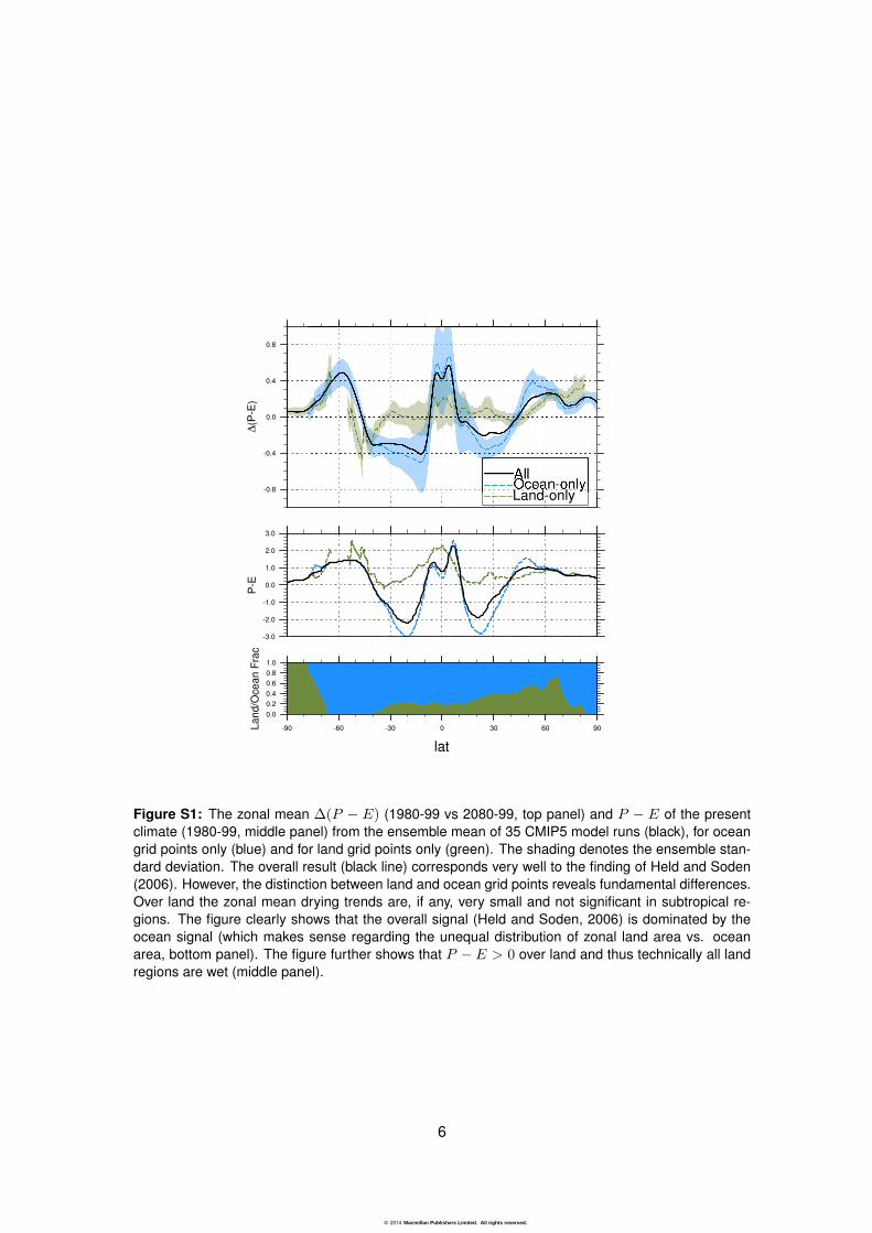
Figure S1: The zonal mean ∆(P − E) (1980-99 vs 2080-99, top panel) and P − E of the presentclimate (1980-99, middle panel) from the ensemble mean of 35 CMIP5 model runs (black), for oceangrid points only (blue) and for land grid points only (green). The shading denotes the ensemble stan-dard deviation. The overall result (black line) corresponds very well to the finding of Held and Soden(2006). However, the distinction between land and ocean grid points reveals fundamental differences.Over land the zonal mean drying trends are, if any, very small and not significant in subtropical re-gions. The figure clearly shows that the overall signal (Held and Soden, 2006) is dominated by theocean signal (which makes sense regarding the unequal distribution of zonal land area vs. oceanarea, bottom panel). The figure further shows that P − E > 0 over land and thus technically all landregions are wet (middle panel).

6


C Evaluation for the 1948-2005 period

To assess the sensitivity of the results on the time period chosen for the evaluation, and forconsistency with our analysis of dryness changes over the 1948-2005 period, we evaluate here9 E and 4 observations-based P datasets together with 11 estimates of Ep over the 1948-2005period, resulting in a total number of 396 combinations. The validation is performed using thesame methodology as for the 1984-2005 period (see Methods and Table S1, S2 and S3).The RMSwE’s of all combinations containing a certain E, P or Ep dataset are shown in Fig. S2.Most E datasets that are found at the top of the panel (i.e. with smallest RMSwE’s) also displaythe smallest RMSwE’s for the short analysis period (Fig. 2) and show lower error measurescompared to those at the bottom of the panel, independently of the choice of P and Ep. Thelargest median RMSwE (1.75, see the boxplot for the NCEP Reanalysis in Fig. S2a) is almosteight times larger than the lowest value (0.23 for the VIC LSM). Here, E datasets are clearlysubdivided into two performance categories, whereby eight of the nine data sets with relativelylow median values belong to the category of LSMs driven by an observations based forcing(green and blue color). The effect of the choice of the P and Ep datasets is on the contraryalmost negligible. However, the results are very similar compared to those shown in the main textand underline the robustness of our methodology.

Figure S2: Budyko validation of hydrological dataset combinations for the 1948-2005 period. Boxplotsof all RMSwEs related either to a) an individual E or b) P dataset and c) the Ep estimates. Colors forthe E datasets denote the different classes (Mueller et al., 2011): LSMs with various forcings: green,LSMs from the TRENDY project (Sitch et al., 2013) (TR): blue, reanalysis: yellow. Dashed verticallines illustrate the absolute minimum, the overall median and absolute maximum RMSwE (from left toright). See text and Methods for more information

7


D Dryness changes analysis for other time periods

In our study, we detect changes in the mean hydroclimatological conditions between the time pe-riods 1948 to 1968 and 1985 to 2005. Changes on shorter time scales are potentially influencedby internal climate variability and are thus not used to detect long-term trends. However, in theinterest of completeness we performed the same analysis comparing the first (1948-1968) andthe last period (1985-2005) with the respective middle period (1968-1985, see Fig. S3).Comparing the first two periods reveals drying trends across the Sahel and other parts of Africa, inEast Asia and the Mediterranean. Wetting appears in parts of North and South America, NorthernEurope, West Asia and North Australia.Comparing the last periods shows drying trends in many parts of Central Africa, Northeast Brazil,Mexico, the Mediterranean, the Middle East and various parts of Asia. Wetting trends are foundin some parts of South America, the eastern US, northern Asia and the Sahel region.Following these results, strongest changes took place between the first and the middle periodand are just partly intensified between the last periods. However, some regions showing non-significant long-term trends experienced significant wetting first, followed by significant drying(like e.g. in Mexico or Middle East/Central Asia), possibly caused by internal variations.

Figure S3: Drying/wetting trends analysed comparing (a) the 1948-1968 and the 1968-1985 and (b)the 1968-1985 and the 1985-2005 period applying the same methodology as for the long period shownin Fig. 4a. Dark red (dark blue) denotes a significant change towards drier (wetter) conditions bothregarding the land water balance and hydrological regime shifts. Red/orange shows a shift towardsmore arid conditions. Drying due to changes in the land water balance only is depicted by green/pinkcolor

8


E Sensitivity to the choice of the significance level

Our analysis was conducted using a significance level of 5% (p < 0.05). Choosing a differentsignificance level (see Supplementary Methods) certainly affects the amount of total land areaexperiencing significant changes (for p < 0.01: 86.4% and for p < 0.1: 67.7%). Shown inFig. S4 and Fig. S5 are results obtained by performing the analysis with p < 0.01 and p < 0.1.The basic findings remain similar, apart from the expected increase/decrease of total area withsignificant change. However, the results underline the robustness of the DDWW evaluation, asthe percentage of global land with valid or invalid DDWW is independent from the choice of thesignificance level

Figure S4: Same as Fig. 4, but with setting the significance level to 1% (p < 0.01).

9


Figure S5: Same as Fig. 4, but with setting the significance level to 10% (p < 0.1).

10


F Alternative dryness change analysis

In order to assess the robustness of the outcomes from our dryness change analysis we directlyinvestigate changes in ∆(P − E) and the aridity index ∆(Ep/P ). These measures are one-dimensional, requiring other test statistics. For Ep/P (and P − E analogously) the empiricaldistribution generated by all possible Ep/P combinations of a particular period is unknown, wetherefore use a bootstrap hypothesis test to identify significant changes. We resample the mediandifference between both periods (48-68 vs. 85-05) ∆(Ep/P ) 1000 times by drawing bootstrapsamples from the merged sample of both periods and calculating ∆(Ep/P )′ for each sample.If ∆(Ep/P )′ > ∆(Ep/P ) if ∆(Ep/P ) < 0 (or vice versa) occurs less than 5 times (p < 0.01),we consider ∆(Ep/P ) as significantly different from 0. The same approach identifies significantchanges in P − E.The results shown in Fig. S6 are qualitatively similar to those shown in Fig. 4. Both methodsreveal significant trends in the same regions, but the overall area of significant change is largerfor thealternative test (18% vs. 24.6%). This is due to different statistical power of each test and dif-ferent significance levels. However, the use of different significance levels does not change thedistribution of area fraction supporting or not-supporting the DDWW paradigm (not shown).Furthermore, other test statistics like a classical two-sample t-test (which is not a good choicesince normality is not always given) or the non-parametric Kolmogorov-Smirnov test (which has arather low statistical power) show similar results (not shown). Hence, our findings are robust anddo not depend on the choice of test statistics.

11


Figure S6: Investigating the DDWW paradigm by analysing ∆-changes in P − E and Ep/P . a)Significant drying/wetting trends computed at the grid box level with significance determined via abootstrap hypothesis test. b) Distribution of arid (orange) to humid (blue ) areas within the periodfrom 1948-1968. 2 c) Comparing the changes in a) with the hydrological conditions of the 1948-1968period in b) evaluates the‘dry gets drier, wet gets wetter’ paradigm.

12


References

Adler, R. F., Huffman, G. J., Chang, A., Ferraro, R., Xie, P., Janowiak, J., Rudolf, B., Schneider, U.,Curtis, S., Bolvin, D., Gruber, A., Susskind, J., Arkin, P., and Nelkin, E. (2003). The version-2global precipitation climatology project (GPCP) monthly precipitation analysis (1979-present).J. Hydrometeor., 4:1147–1167.

Blaney, H. and Criddle, W. (1964). Determining water requirements for settling water disputes.Nat. Resources J., 4:29.

Budyko, M. I. (1974). Climate and life. Academic Press, New York.

Chen, F. and Dudhia, J. (2001). Coupling an advanced land surface-hydrology model with thepenn state-NCAR MM5 modeling system. part i: Model implementation and sensitivity. Mon.Wea. Rev., 129(4):569–585.

Chen, M., Xie, P., Janowiak, J., and Arkin, P. (2002). Global land precipitation: A 50-yr monthlyanalysis based on gauge observations. J. of Hydromet., 3(3):249–266.

Compo, G. P., Whitaker, J. S., Sardeshmukh, P. D., Matsui, N., Allan, R. J., Yin, X., Gleason,B. E., Vose, R. S., Rutledge, G., Bessemoulin, P., Bronnimann, S., Brunet, M., Crouthamel,R. I., Grant, A. N., Groisman, P. Y., Jones, P. D., Kruk, M. C., Kruger, A. C., Marshall, G. J.,Maugeri, M., Mok, H. Y., Nordli, A., Ross, T. F., Trigo, R. M., Wang, X. L., Woodruff, S. D., andWorley, S. J. (2011). The twentieth century reanalysis project. Quarterly Journal of the RoyalMeteorological Society, 137(654):1–28.

Cox, P. (2001). Description of the triffid dynamic global vegetation model. Hadley Centre TechnicalNote, 24:1–16.

Dee, D., Uppala, S., Simmons, A., Berrisford, P., Poli, P., Kobayashi, S., Andrae, U., Balmaseda,M., Balsamo, G., Bauer, P., et al. (2011). The ERA-Interim reanalysis: Configuration andperformance of the data assimilation system. Q. J. R. Meteorol. Soc., 137(656):553–597.

Ek, M., Mitchell, K., Lin, Y., Rogers, E., Grunmann, P., Koren, V., Gayno, G., and Tarpley, J. (2003).Implementation of noah land surface model advances in the national centers for environmentalprediction operational mesoscale eta model. J. Geophys. Res, 108(D22):8851.

Fu, B. (1981). On the calculation of the evaporation from land surface (in chinese),. Sci. Atmos.Sin., 1(5):23–31.

Harris, I., Jones, P., Osborn, T., and Lister, D. (2013). Updated high-resolution grids of monthlyclimatic observations - the CRU TS3.10 dataset. International Journal of Climatology.

Held, I. M. and Soden, B. J. (2006). Robust responses of the hydrological cycle to global warming.Journal of Climate, 19(21):5686–5699.

Jung, M., Reichstein, M., Ciais, P., Seneviratne, S. I., Sheffield, J., Goulden, M. L., Bonan, G.,Cescatti, A., Chen, J., de Jeu, R., Dolman, A. J., Eugster, W., Gerten, D., Gianelle, D., Go-bron, N., Heinke, J., Kimball, J., Law, B. E., Montagnani, L., Mu, Q., Mueller, B., Oleson, K.,Papale, D., Richardson, A. D., Roupsard, O., Running, S., Tomelleri, E., Viovy, N., Weber, U.,Williams, C., Wood, E., Zaehle, S., and Zhang, K. (2010). Recent decline in the global landevapotranspiration trend due to limited moisture supply. Nature, 467:951 – 954.

13


Kanamitsu, M., Ebisuzaki, J., Woollen, J., Yang, S.-K., Hnilo, J. J., Fiorino, M., and Potter, G. L.(2002). NCEP-DOE AMIP-II reanalysis (r-2). Bull. Amer. Meteor. Soc., 83:1631–1643.

Legates, D. and Willmott, C. (1990a). Mean seasonal and spatial variability in gauge-corrected,global precipitation. Int. J. Clim, 10(2):111–127.

Legates, D. and Willmott, C. (1990b). Mean seasonal and spatial variability in global surface airtemperature. Theo. and Appl. Clim., 41(1):11–21.

Leuning, R., Zhang, Y., Rajaud, A., Cleugh, H., and Tu, K. (2008). A simple surface conductancemodel to estimate regional evaporation using MODIS leaf area index and the penman-monteithequation. Water Resources Research, 44(10):W10419.

Levy, P., Cannell, M., and Friend, A. (2004). Modelling the impact of future changes in climate,CO2 concentration and land use on natural ecosystems and the terrestrial carbon sink. GlobalEnvironmental Change, 14(1):21–30.

Li, D., Pan, M., Cong, Z., Zhang, L., and Wood, E. (2013). Vegetation control on water and energybalance within the budyko framework. Water Resources Research, 49(2):969–976.

Liang, X., Lettenmaier, D., Wood, E., and Burges, S. (1994). A simple hydrologically based modelof land surface water and energy fluxes for general circu-lation models. J. Geophys. Res,99:14415–14428.

Maidment, D. R. (1993). Handbook of hydrology. McGraw-Hill.

Miralles, D., Holmes, T., De Jeu, R., Gash, J., Meesters, A., and Dolman, A. (2011). Global land-surface evaporation estimated from satellite-based observations. Hydrology and Earth SystemSciences, 15(2):453–469.

Monteith, J. (1965). Evaporation and environment. In Symp. Soc. Exp. Biol, volume 19, page 4.

Mueller, B., Seneviratne, S., Jimenez, C., Corti, T., Hirschi, M., Balsamo, G., Ciais, P., Dirmeyer,P., Fisher, J., Guo, Z., et al. (2011). Evaluation of global observations-based evapotranspirationdatasets and IPCC AR4 simulations. Geophys. Res. Lett., 38(6):L06402.

Murray, F. W. (1967). On the computation of saturation vapor pressure. Journal of Applied Mete-orology, 6(1):203–204.

Oleson, K., Lawrence, D., Gordon, B., Flanner, M., Kluzek, E., Peter, J., Levis, S., Swenson, S.,Thornton, E., Feddema, J., et al. (2010). Technical description of version 4.0 of the communityland model (CLM). NCAR Technical Note, (NCAR/TN-478+STR,):257pp.

Peel, M. C., Finlayson, B. L., and McMahon, T. A. (2007). Updated world map of the koppen-geiger climate classification. Hydrology and Earth System Sciences, 11(5):1633–1644.

Priestley, C. and Taylor, R. (1972). On the assessment of surface heat flux and evaporation usinglarge-scale parameters. Monthly weather review, 100(2):81–92.

Rienecker, M. M., Suarez, M. J., Gelaro, R., Todling, R., Bacmeister, J., Liu, E., Bosilovich, M. G.,Schubert, S. D., Takacs, L., Kim, G.-K., Bloom, S., Chen, J., Collins, D., Conaty, A., da Silva,A., Gu, W., Joiner, J., Koster, R. D., Lucchesi, R., Molod, A., Owens, T., Pawson, S., Pegion,

14


P., Redder, C. R., Reichle, R., Robertson, F. R., Ruddick, A. G., Sienkiewicz, M., and Woollen,J. (2011). MERRA: NASA’s modern-era retrospective analysis for research and applications.Journal of Climate, 24(14):3624–3648.

Rubel, F. and Kottek, M. (2010). Observed and projected climate shifts 1901-2100 depicted byworld maps of the koppen-geiger climate classification. Meteorologische Zeitschrift, 19(2):135–141.

Rudolf, B., Beck, C., Grieser, J., and Schneider, U. (2005). Global precipitation analysis products.global precipitation climatology centre (GPCC). DWD, Internet Publication:1 –8.

Saha, S., Moorthi, S., Pan, H., Wu, X., Wang, J., Nadiga, S., Tripp, P., Kistler, R., Woollen, J.,Behringer, D., et al. (2010). The NCEP climate forecast system reanalysis. Bulletin of theAmerican Meteorological Society, 91(8):1015–1057.

Sheffield, J., Goteti, G., and Wood, E. (2006). Development of a 50-year high-resolution globaldataset of meteorological forcings for land surface modeling. J. Clim., 19(13):3088–3111.

Sheffield, J., Wood, E., and Roderick, M. (2012). Little change in global drought over the past 60years. Nature, 491:435–438.

Sitch, S., Friedlingstein, P., Gruber, N., Jones, S., Murray-Tortarolo, G., Ahlstrom, A., Doney, S.,Graven, H., Heinze, C., Huntingford, C., Levis, S., Levy, P. E., Lomas, M., Poulter, B., et al.(2013). Trends and drivers of regional sources and sinks of carbon dioxide over the past twodecades. Global Change Biology, (submitted).

Smith, B., Prentice, I., and Sykes, M. (2001). Representation of vegetation dynamics in themodelling of terrestrial ecosystems: comparing two contrasting approaches within europeanclimate space. Global Ecology and Biogeography, 10(6):621–637.

Thornthwaite, C. (1948). An approach toward a rational classification of climate. Geographicalreview, 38(1):55–94.

Tucker, C. J., Pinzon, J. E., Brown, M. E., Slayback, D. A., Pak, E. W., Mahoney, R., Vermote, E. F.,and El Saleous, N. (2005). An extended AVHRR 8 km NDVI dataset compatible with MODISand SPOT vegetation NDVI data. International Journal of Remote Sensing, 26(20):4485–4498.

Weiß, M. and Menzel, L. (2008). A global comparison of four potential evapotranspiration equa-tions and their relevance to stream flow modelling in semi-arid environments. Advances inGeosciences, 18:15–23.

Woodward, F. and Lomas, M. (1995). Vegetation-dynamics simulating responses to climatechange. Glob. Biogeochem. C., 9:471–490.

Zaehle, S., Ciais, P., Friend, A. D., and Prieur, V. (2011). Carbon benefits of anthropogenicreactive nitrogen offset by nitrous oxide emissions. Nature Geoscience, 4(9):601–605. 00039.

Zaehle, S. and Friend, A. (2010). Carbon and nitrogen cycle dynamics in the O-CN land surfacemodel, I: Model description, site- scale evaluation and sensitivity to parameter estimates. Glob.Biogeochem. C., 24(1):GB1005.

15


Zhang, Y., Leuning, R., Hutley, L., Beringer, J., McHugh, I., and Walker, J. (2010). Using of long-term water balances to parameterise surface conductance and calculate evaporation at 0.5◦

spatial resolution. Water Resources Research, 46(W05512):14 PP.

16


global assessment of trends in wetting and drying wetting ... · supplementary information: global...

Documents