giuseppe cortese, kjell r. bjørklund & jane k. dolven ... · koc¸-karpuz & schrader...

Polycystine radiolarians in the Greenland–Iceland–Norwegian Seas: speciesand assemblage distribution

Giuseppe Cortese, Kjell R. Bjørklund & Jane K. Dolven

Cortese G, Bjørklund KR, Dolven JK. 2003. Polycystine radiolarians in the Greenland–Iceland–Norwegian Seas: species and assemblage distribution. Sarsia 88:65–88.

SARSIA

Cluster analysis and Q-mode factor analysis have been applied to polycystine radiolarian census datafrom 160 core-top samples. This allowed us to recognize four faunal assemblages in the Greenland–Iceland–Norwegian Seas, each related to different oceanographic conditions. A regression equation forderiving palaeotemperatures from these assemblages has also been developed. The standard error ofestimate for this equation is �1.2°C. The relative abundance of the species having the higher loadingsin the core-top assemblages has been mapped, in order to identify and analyse water mass andenvironmental requirements for these species. Cluster analysis has also been performed on the samedata set, providing results which are in good harmony with those derived by Q-mode factor analysis.

Giuseppe Cortese, Alfred Wegener Institute for Polar and Marine Research (AWI), Columbusstrasse,P.O. Box 120161, DE-27515 Bremerhaven, Germany.Kjell R. Bjørklund & Jane K. Dolven, Paleontological Museum, University of Oslo, Sars gate 1,NO-0562 Oslo, Norway.E-mail: [email protected]; [email protected]; [email protected]

Keywords: radiolaria; Greenland–Iceland–Norwegian Seas; distribution; factor analysis; clusteranalysis; palaeotemperatures.

INTRODUCTION

The biogeographical distribution of microfossil specieshas been widely used in palaeontology in order torecognize faunal provinces and trace their positionthrough time. When trying to extract palaeo-environ-mental information (e.g. the correlation between therelative percentage of a species and water temperature,or any other environmental variable) from a species’relative abundance at different stations, a simple x–ygraph can be used as a rudimentary tool.

Increasingly more complex data sets containing ahigh number of species and stations require moresophisticated techniques, such as those that have beendeveloped in the last decades to allow the description,simplification and interpretation of vast data sets. Theseso-called “multivariate techniques” (principal compo-nent analysis, correspondence analysis, cluster analysis,among others) are based on different algorithms, andcan therefore be used jointly to stress different aspectsof the data set, and to draw different, but closely related,conclusions.

In this paper we will use the factor analysis method(Imbrie & Kipp 1971) together with cluster analysis anddescribe what can be gained by the application of thesemethods to radiolarian census data from the surfacesediments of the Greenland–Iceland–Norwegian (GIN)Seas.

Transfer functions for estimating mean surface ocean

temperatures for the Norwegian Sea have been derivedfor planktonic foraminifera (Kellogg 1976), diatoms(Koc-Karpuz & Schrader 1990; Koc & al. 1993) andradiolarians (Bjørklund & al. 1998). The planktonicforaminifera assemblage (Kellogg 1976) of the GINSeas is almost monospecific, with 95% Neogloboqua-drina pachyderma (dextral) (Ehrenberg), while Neo-globoquadrina pachyderma (sinistral) (Ehrenberg) andfour additional species are common: Globigerinabulloides d’Orbigny, Globigerina quinqueloba Nat-land, Globorotalia inflata (d’Orbigny), and Globiger-inita glutinata (Egger). Koc-Karpuz & Schrader (1990)used about 70 species to define surface diatom associa-tions from the North Atlantic and the GIN Seas, and toextract palaeotemperature estimates for the last 13.514C ka (Koc & al. 1993, 1996).

Bjørklund & al. (1998) identified 75 radiolarian taxain the GIN Seas surface sediments, while Samtleben &al. (1995) reported on 50 species from the sediment and60 species from the plankton. In this study we haveidentified 114 radiolarian taxa, making the radiolariansthe most diversified microplankton group, both inplankton and sediments, in the GIN Seas. The radi-olarian data set developed by Bjørklund & al. (1998)was used to derive a palaeotemperature transfer func-tion that was applied to a 13.5 ka long record from thesoutheastern Norwegian Basin (Dolven 1998).

In the present work we develop a new palaeotem-perature equation for the GIN Seas, based on poly-

DOI 10.1080/00364820310000274 � 2003 Taylor & Francis

Published in collaboration with the University of Bergen and the Institute of Marine Research, Norway

cystine radiolarians. This represents a considerableimprovement over previously published work, as thecurrent study is based on 114 taxa [compared with 75taxa in Bjørklund & al. (1998)] and 160 core-topsamples [compared with 63 samples in Bjørklund & al.(1998) and Dolven (1998)].

We include in the reference data set a greatergeographical area (large portions of the GreenlandSea and the northern North Atlantic were not covered inprevious studies) and a larger temperature range than inBjørklund & al. (1998). By doing so, we expand therange of applicability of the present calibration data set,and improve the accuracy of palaeotemperature esti-mates in the GIN Seas.

Moreover, it has now been possible to recognize aGreenland Sea–Lofoten Basin faunal assemblage thatseems to be related not only to sea surface temperature,but also to a variety of oceanographic variables, such asbasin bathymetry, sea ice regime and processes, andopal dissolution at the bottom.

MATERIAL AND METHODS

Most of the core-top material used in this study wasobtained from Christian-Albrechts University, Kiel,Germany (collected on RVs Polarstern and Meteor),the topmost 1–2 cm of the Trigger weight cores fromthe core libraries at the Lamont-Doherty Earth Obser-vatory, Columbia University (RV Vema cruises 23, 27,28, 29, and 30), and the Department of Oceanography,University of Washington (USS Edisto 1963 cruise).Two additional core-tops were made available to usfrom the Geological Institute, University of Bergen (RVHakon Mosby cruise 31).

The reference data set includes 160 stations (filledcircles in Fig. 1, asterisks in Table 1), extends from theFram Strait to the Rockall Plateau area, documenting allthe temperature and oceanographic regimes included, inthe study area, between ca 55 and 80°N. The core-topsamples used for the reference data set were chosen(from a total of 344 core-tops available) based on threecriteria, in order of importance:

� samples with low abundance or barren of radiolarianskeletons were excluded;

� samples with very low communalities, indicative ofpoor preservation or reworked faunas, in preliminaryfactor analysis runs were excluded;

� samples significantly extending the geographicalcoverage of the reference data set were included.

The techniques used to separate the radiolarian skele-tons from the sediment have been described previously

by Goll & Bjørklund (1974). The sediment wasdisaggregated using hydrogen peroxide, and a constantvolume of the screened residue (45 �m mesh size)mounted on a slide with Canada Balsam. We counted,in arbitrarily selected fields of view, between 261 and502 specimens identified to the species level or to thelowest level possible. The resulting numbers includedSpumellarida indet. (not identified) and Nassellaridaindet. These two groups are negligible in some areas,constituting less than 5% of the total fauna, while inother areas they can be quite significant in numbers,often mainly juveniles (in areas with high values ofradiolarians g�1, low opal refraction index) andfragmented larcoids (in areas with low values ofradiolarians g�1, high opal refraction index).

In total, 114 species have been recognized by trans-mitted light microscopy. The species that were treatedstatistically had to occur with more than 2% of the totalfauna in at least one station, as recommended by Imbrie& Kipp (1971).

In the GIN Seas we have recognized three morpho-types of the genus Pseudodictyophimus: P. gracilipesgracilipes, P. g. bicornis, and P. g. multispina. We havenot been consistent during our work in identifying thethree Pseudodictyophimus morphotypes, so we havechosen to list them as the Pseudodictyophimus graci-lipes group. Several species common in the warm andtransitional water regimes of the North Atlantic(Euchitonia spp., Lamprocyclas maritalis, Spongocore

Fig. 1. Location of all the core-top samples examined in thisstudy. The stations marked with a full circle have beenincluded in the factor and cluster analyses.

66 Sarsia 88:65-88 – 2003

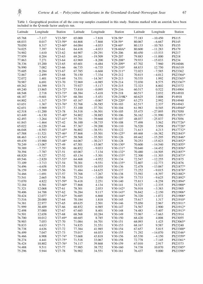
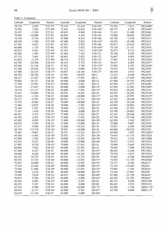
Table 1. Geographical position of all the core-top samples examined in this study. Stations marked with an asterisk have beenincluded in the Q-mode factor analysis run.

Latitude Longitude Station Latitude Longitude Station Latitude Longitude Station

65.768 �7.117 V23-58* 65.000 �7.818 V28-58* 77.183 �10.450 PS11568.033 0.017 V23-59* 64.868 �7.868 V28-59* 80.067 �6.667 PS14570.050 8.317 V23-60* 64.084 �4.033 V28-60* 80.133 �10.783 PS15574.025 7.397 V23-61 64.418 �4.033 V28-60A* 80.600 �11.283 PS17974.902 1.610 V23-62 64.907 �29.291 V29-206 80.450 �13.533 PS21777.959 0.204 V23-63 69.261 �19.509 V29-207 79.883 �11.000 PS21877.863 7.271 V23-64 63.969 �8.200 V29-208* 79.933 �15.033 PS23478.336 15.200 V23-65 65.601 �6.484 V29-209* 67.702 7.960 PS1604676.990 7.082 V23-66 66.735 �6.735 V29-210* 68.833 12.750 PS1631975.605 0.284 V23-67 67.785 �6.668 V29-211* 72.023 �7.585 PS2336272.867 �2.499 V23-68 70.150 �7.334 V29-212 70.815 �4.012 PS23364*72.072 1.401 V23-69 74.351 �14.367 V29-213 70.535 1.992 PS23365*70.987 6.691 V23-70 72.969 �6.985 V29-214 72.030 8.575 PS23367*69.262 14.399 V23-71 75.927 �5.117 V29-215 72.323 8.802 PS2337269.240 13.865 V23-72* 73.810 �0.095 V29-216 60.517 0.522 PS1490468.548 2.718 V23-73* 68.384 �5.418 V29-218 60.517 2.032 PS1491068.187 �9.601 V23-74* 68.384 �5.451 V29-219K* 60.625 3.008 P1491864.802 �1.317 V23-75* 65.167 �0.067 V29-220* 63.273 2.992 PS1494063.651 1.367 V23-76* 52.768 �36.585 V30-103 62.517 2.337 PS1494362.651 �5.969 V23-77 53.100 �37.701 V30-104 61.983 0.545 PS14944*62.518 �11.200 V23-78 54.518 �36.501 V30-105 55.475 �27.895 PS1705063.449 �6.130 V27-40* 54.802 �38.885 V30-106 56.162 �31.990 PS17051*62.493 �3.264 V27-41* 55.701 �39.668 V30-107 48.037 �25.837 PS1705661.843 �1.464 V27-42 56.100 �38.735 V30-108 77.498 3.562 PS17726*65.022 �6.220 V27-44 57.367 �39.200 V30-110 76.520 3.958 PS17728*66.048 �8.593 V27-45* 56.802 �38.551 V30-122 71.613 4.213 PS17732*67.588 �11.521 V27-46* 57.868 �35.501 V30-125* 69.468 �16.382 PS21843*68.463 �13.543 V27-47* 58.568 �35.501 V30-126 69.442 �15.295 PS21846*69.439 �15.900 V27-48* 64.067 �30.217 V30-128 70.253 �15.823 PS21852*70.249 �13.067 V27-49 67.501 �15.067 V30-130* 70.600 �14.540 PS21855*70.389 �7.757 V27-50 66.852 �9.033 V30-131* 70.640 �14.452 PS21856*70.394 �7.787 V27-51 65.067 �7.134 V30-132* 70.480 �14.505 PS21857*68.820 �9.327 V27-52 65.134 �5.301 V30-133* 72.300 �11.303 PS21873*69.546 �2.820 V27-53* 64.468 �4.952 V30-134 72.547 �12.255 PS2187573.109 �3.713 V27-54 70.301 �9.551 V30-135* 72.807 �12.773 PS2187674.496 �4.658 V27-55 70.935 �16.935 V30-136 72.478 �13.067 PS21877*76.159 �5.399 V27-56 71.484 �14.635 V30-137 73.252 �9.015 PS21878*74.466 �1.691 V27-57 75.768 �7.267 V30-138 73.592 �8.397 PS21882*73.541 2.665 V27-58 75.234 �3.050 V30-139 73.733 �9.625 PS21892*73.070 4.822 V27-59* 76.418 2.251 V30-140 75.813 �8.258 PS21894*72.184 8.581 V27-60* 77.868 4.134 V30-141 74.527 �2.335 PS21900*71.321 12.068 V27-61 78.301 2.033 V30-142* 76.918 �3.383 PS2190570.406 14.788 V27-62 76.284 9.117 V30-143* 76.842 �2.150 PS21906*70.424 12.077 V27-63* 76.685 6.868 V30-144* 76.320 �1.072 PS21908*73.516 20.000 V27-64 70.184 1.818 V30-145 75.617 1.317 PS21910*74.381 22.977 V27-65 69.635 2.501 V30-146 75.050 2.967 PS21911*71.999 30.409 V27-66 68.852 6.985 V30-147 74.567 2.900 PS21912*72.498 37.000 V27-67 67.685 8.401 V30-148 74.483 �5.407 PS21913*74.501 12.658 V27-68 68.568 10.284 V30-149 73.967 �7.663 PS2191476.700 10.012 V27-69* 68.685 8.785 V30-150 68.420 4.008 PS2305578.903 7.053 V27-70 71.084 16.701 V30-151 68.093 1.425 PS23065*78.833 4.633 V27-71 74.835 31.551 V30-153 68.167 9.587 PS2324078.738 4.636 V27-72 77.384 41.985 V30-154 67.657 5.815 PS23300*76.499 7.047 V27-73 75.017 44.033 V30-155 71.292 �14.070 PS23346*76.466 6.908 V27-74* 73.668 43.818 V30-156 65.530 �4.150 PS23359*78.274 4.441 V27-75* 71.518 33.067 V30-158 72.778 �7.145 PS23361*76.424 10.802 V27-76* 74.117 39.868 V30-159 67.010 2.917 PS2337374.488 9.511 V27-77 77.985 38.752 V30-160 74.738 10.870 PS23385*75.296 5.944 V27-78 76.902 34.551 V30-161 76.437 9.000 PS23398*

Cortese & al. – Polycystine radiolarians in the Greenland–Iceland–Norwegian Seas 67

Latitude Longitude Station Latitude Longitude Station Latitude Longitude Station

78.119 3.625 V27-79 75.334 23.434 V30-162 72.352 �7.813 PS23400*78.392 7.424 V27-80* 72.401 14.818 V30-163* 68.737 0.155 PS23402*76.247 �2.394 V27-81 69.835 8.969 V30-164 71.413 21.490 PS2340474.995 �10.808 V27-82 68.969 4.418 V30-165 75.000 28.003 PS2340774.194 �5.716 V27-83 67.000 6.534 V30-166 65.798 �3.510 PS23411*68.630 �1.596 V27-84* 67.000 5.852 V30-167* 54.835 �18.380 PS2341367.362 4.027 V27-85 67.267 5.835 V30-168 50.673 �19.435 PS2341766.608 1.119 V27-86 67.501 5.852 V30-169* 74.130 21.147 PS2342862.937 4.281 V27-93* 67.267 7.017 V30-170* 76.475 8.737 PS23453*66.289 1.493 V27-94* 67.468 7.367 V30-171 76.748 8.195 PS23454*67.135 3.481 V27-95 68.401 5.852 V30-172 76.867 8.405 PS23455*61.010 �4.339 V27-96* 68.334 5.752 V30-173 77.067 6.363 PS23456*64.785 �29.568 V28-14* 68.167 5.752 V30-174 76.637 6.405 PS23457*65.284 �31.334 V28-15 67.852 5.768 V30-175* 75.992 6.357 PS23458*67.100 �25.618 V28-16* 67.167 6.084 V30-176 75.875 5.482 PS2345967.500 �24.233 V28-17* 54.067 �24.184 V30-177 66.670 4.913 PS2346768.785 �20.768 V28-18 67.501 �18.835 ED-1 71.633 �8.450 PS2347868.217 �15.267 V28-19* 67.000 �17.501 ED-2 67.892 �17.920 PS23481*70.802 �18.317 V28-20 69.000 0.000 ED-12 67.890 �18.763 PS23482*71.768 �15.501 V28-21* 69.000 �2.501 ED-13 67.658 �11.077 PS2348872.434 �13.651 V28-22 69.000 �5.000 ED-14* 67.505 �12.502 PS23489*74.518 �13.117 V28-23 69.000 �7.501 ED-15* 65.032 �28.282 PS2351675.167 �10.868 V28-24 69.501 �8.501 ED-16 64.542 �28.203 PS23518*76.818 �1.334 V28-25 69.000 �10.000 ED-17* 64.798 �29.597 PS23519*76.217 �0.701 V28-26* 69.501 �11.251 ED-18* 63.762 �28.658 PS23522*75.752 �0.885 V28-27 70.000 �10.000 ED-19 62.250 �30.220 PS23523*73.484 �0.835 V28-28 70.000 �7.501 ED-21* 63.003 �29.903 PS23524*72.184 5.267 V28-29 70.000 �2.501 ED-24 63.248 �27.597 PS23525*71.167 1.618 V28-30 70.000 0.000 ED-25 63.398 �28.062 PS23526*66.451 2.167 V28-31* 71.000 �2.501 ED-27 63.163 �28.840 PS23528*64.785 4.301 V28-32* 71.000 �7.501 ED-29 63.740 �25.740 PS23536*62.902 0.585 V28-33* 71.000 �10.000 ED-30* 62.050 2.502 PS2353764.835 �3.585 V28-34 71.000 �13.000 ED-32 75.000 �0.007 PS2354867.117 �9.568 V28-35* 71.000 �19.251 ED-34 75.057 �4.598 PS23549*68.718 �12.718 V28-36* 70.501 �16.000 ED-36 69.060 �20.510 PS2355372.067 �9.067 V28-37 70.551 �13.251 ED-37* 69.990 3.987 PS31/002*69.384 �4.401 V28-38* 70.501 �11.251 ED-38* 74.943 �11.175 PS31/02467.885 �1.935 V28-39* 70.000 �12.501 ED-39* 78.933 �5.195 PS37/00867.635 0.251 V28-40 70.000 �15.000 ED-40* 78.975 �3.973 PS37/01267.685 0.234 V28-41* 70.000 �17.501 ED-41 78.990 �5.665 PS37/01468.084 3.852 V28-42* 69.000 �23.501 ED-43 78.965 �7.688 PS37/01667.200 6.167 V28-43 69.000 �17.501 ED-47* 80.022 �4.248 PS37/02168.668 6.618 V28-44* 69.000 �14.301 ED-49* 79.570 �3.873 PS37/02268.334 10.735 V28-45 69.501 �13.752 ED-50 75.002 �6.760 PS44/019*69.701 13.334 V28-46* 69.000 �12.501 ED-51* 74.853 �11.745 PS44/02070.367 16.000 V28-47 68.000 �12.501 ED-52* 74.177 �0.392 PS2613*73.334 12.484 V28-48* 68.000 �15.000 ED-53* 73.155 �19.485 PS264174.484 11.668 V28-49* 68.000 �17.501 ED-54* 75.005 �7.203 PS2616*74.000 4.234 V28-50 68.000 �20.000 ED-55* 73.160 �15.967 PS262873.050 5.818 V28-51* 66.033 �9.868 ED-60* 67.868 �21.758 PS2644*70.935 9.384 V28-52* 66.000 �5.000 ED-62* 68.395 �21.395 PS2645*69.284 8.985 V28-53* 67.000 �2.501 ED-63 80.733 8.050 PS55/10068.251 5.367 V28-54 64.000 8.000 ED-69 80.483 2.933 PS55/15165.518 0.200 V28-55* 65.000 �10.000 ED-77* 64.500 �1.250 HM31-35*68.033 �6.117 V28-56* 63.000 �2.501 ED-87* 63.750 0.000 HM31-3764.635 �11.150 V28-57 63.000 �5.000 ED-88*

Table 1. Continued.

68 Sarsia 88:65-88 – 2003

puella, Theocorythium trachelium) are found in theGIN Seas. They are too rare to be of any importance asindividual species, but as a warm water group they mayshow a more significant distribution pattern. We there-fore grouped them as “Drift fauna” in our species list.Finally, Spongotrochus glacialis, Spongopyle osculosaand Spongopyle resurgens are common in our material.However, as most of them are juvenile stages, we have

not with confidence been able to separate these species.Spongotrochus glacialis being the most commonspecies, we grouped these three spongodiscids as theSpongotrochus group.

Moreover, Artostrobus annulatus and Cycladophoradavisiana have not been considered when developingthe palaeotemperature regression equation, as it hasbeen demonstrated that they live in intermediate or deep

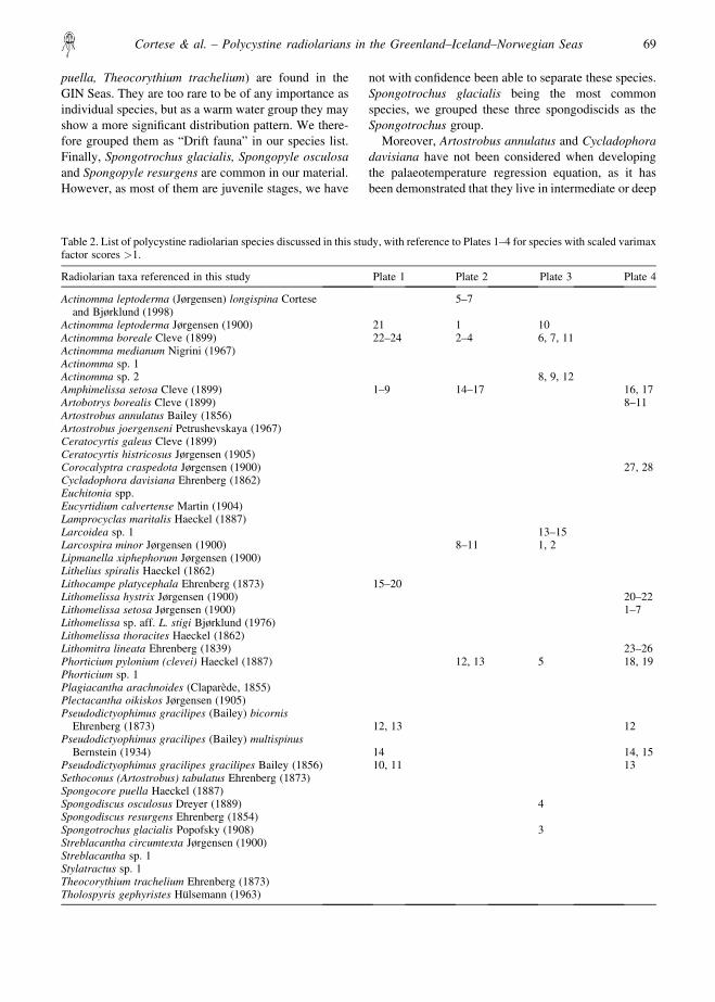
Table 2. List of polycystine radiolarian species discussed in this study, with reference to Plates 1–4 for species with scaled varimaxfactor scores �1.

Radiolarian taxa referenced in this study Plate 1 Plate 2 Plate 3 Plate 4

Actinomma leptoderma (Jørgensen) longispina Corteseand Bjørklund (1998)

5–7

Actinomma leptoderma Jørgensen (1900) 21 1 10Actinomma boreale Cleve (1899) 22–24 2–4 6, 7, 11Actinomma medianum Nigrini (1967)Actinomma sp. 1Actinomma sp. 2 8, 9, 12Amphimelissa setosa Cleve (1899) 1–9 14–17 16, 17Artobotrys borealis Cleve (1899) 8–11Artostrobus annulatus Bailey (1856)Artostrobus joergenseni Petrushevskaya (1967)Ceratocyrtis galeus Cleve (1899)Ceratocyrtis histricosus Jørgensen (1905)Corocalyptra craspedota Jørgensen (1900) 27, 28Cycladophora davisiana Ehrenberg (1862)Euchitonia spp.Eucyrtidium calvertense Martin (1904)Lamprocyclas maritalis Haeckel (1887)Larcoidea sp. 1 13–15Larcospira minor Jørgensen (1900) 8–11 1, 2Lipmanella xiphephorum Jørgensen (1900)Lithelius spiralis Haeckel (1862)Lithocampe platycephala Ehrenberg (1873) 15–20Lithomelissa hystrix Jørgensen (1900) 20–22Lithomelissa setosa Jørgensen (1900) 1–7Lithomelissa sp. aff. L. stigi Bjørklund (1976)Lithomelissa thoracites Haeckel (1862)Lithomitra lineata Ehrenberg (1839) 23–26Phorticium pylonium (clevei) Haeckel (1887) 12, 13 5 18, 19Phorticium sp. 1Plagiacantha arachnoides (Claparede, 1855)Plectacantha oikiskos Jørgensen (1905)Pseudodictyophimus gracilipes (Bailey) bicornis

Ehrenberg (1873) 12, 13 12Pseudodictyophimus gracilipes (Bailey) multispinus

Bernstein (1934) 14 14, 15Pseudodictyophimus gracilipes gracilipes Bailey (1856) 10, 11 13Sethoconus (Artostrobus) tabulatus Ehrenberg (1873)Spongocore puella Haeckel (1887)Spongodiscus osculosus Dreyer (1889) 4Spongodiscus resurgens Ehrenberg (1854)Spongotrochus glacialis Popofsky (1908) 3Streblacantha circumtexta Jørgensen (1900)Streblacantha sp. 1Stylatractus sp. 1Theocorythium trachelium Ehrenberg (1873)Tholospyris gephyristes Hulsemann (1963)


water masses. Six plankton stations (Cleve’s slidecollection at the Swedish Museum of Natural History,Stockholm), sampled during July–September 1898 inthe study area (Bjørklund, unpublished data) confirmthe subsurface habitat of Artostrobus annulatus andCycladophora davisiana, as both species were absentfrom plankton tows shallower than 500 m water depth,while both were present in deeper tows.

After these selection criteria were applied, 34 speciesremained for further analyses. The 34 taxa included inthe factor run in this study are shown in Tables 2 and 3,while the most important species in the four GIN Seafactor groups are shown in Plates 1–4. [The plates figureonly taxa having high factor loadings in the presentpaper. Images and taxonomic references for rarer taxafrom the study area are found in Bjørklund (1976),Schroder-Ritzrau (1995) and Bjørklund & al. (1998).]

The log-transform of the relative abundance of thesespecies, Xlog-transf = ln (X% � 1), was used as the inputmatrix for the Q-mode factor analysis.

Dietrich’s (1969) summer water temperature data setwas used as the source of surface hydrographyinformation, as this atlas provides an accurate andrealistic picture of the distribution of this variable in theGIN Seas. An evaluation of this data set, and why it waspreferred over others, is presented in Bjørklund & al.(1998). Summer temperatures were used, as this is themost likely time of the year for radiolarians toreproduce, and the highest flux of radiolarian skeletonsto the sediments will occur during the summer months.

In fact, in the GIN Seas, the highest opal, carbonateand particulate organic carbon fluxes are observed inthe summer (Peinert & al. 2001). This high exportseason corresponds to late May until September in the

Table 3. Scaled varimax factor scores for the taxa used in this study. Absolute values higher than 1.000 are in bold.

Factor 1 Factor 2 Factor 3 Factor 4

Actinomma leptoderma/boreale group 1.615 4.588 �1.661 0.721Actinomma leptoderma longispina �0.240 1.861 �0.823 �0.284Actinomma medianum 0.019 �0.038 0.234 �0.074Actinomma sp. 1 �0.022 �0.017 �0.050 0.177Actinomma sp. 2 0.083 �0.188 1.091 �0.327Amphimelissa setosa 4.732 �1.252 0.967 �1.310Artobotrys borealis 0.072 �0.521 �0.221 2.388Artostrobus joergenseni 0.897 �0.419 0.144 0.507Ceratocyrtis galeus 0.026 0.026 �0.058 0.244Ceratocyrtis histricosus 0.001 �0.053 �0.078 0.366Corocalyptra craspedota �0.196 �0.162 0.020 1.036Drift fauna �0.043 �0.037 0.225 0.132Eucyrtidium calvertense 0.008 �0.058 0.271 �0.025Larcospira minor �0.409 1.798 3.421 0.015Larcoidea sp. 1 �0.189 �0.270 1.086 0.990Lipmanella xiphephorum �0.054 �0.041 �0.058 0.380Lithelius spiralis �0.064 �0.105 0.032 0.408Lithocampe platycephala 1.731 0.563 �0.273 0.865Lithomelissa hystrix �0.144 �0.237 0.020 1.124Lithomelissa setosa �0.040 �0.929 0.045 3.683Lithomelissa sp. aff. L. stigi �0.046 �0.023 �0.073 0.227Lithomelissa thoracites �0.056 �0.057 �0.056 0.374Lithomitra lineata 0.145 �0.377 0.020 1.217Phorticium pylonium (clevei) �0.284 1.477 1.956 1.273Phorticium sp. 1 0.015 �0.034 0.160 �0.046Plagiacantha arachnoides 0.033 �0.053 �0.013 0.123Plectacantha oikiskos 0.135 �0.110 �0.029 0.331Pseudodictyophimus gracilipes group 2.034 �0.207 0.376 1.577Sethoconus (Artostrobus) tabulatus 0.025 �0.014 �0.001 0.034Spongotrochus glacialis group �0.068 0.624 3.294 �0.296Streblacantha circumtexta �0.128 0.149 0.394 0.150Streblacantha sp. 1 �0.110 �0.184 0.076 0.777Stylatractus sp. 1 0.014 �0.089 0.398 �0.038Tholospyris gephyristes 0.747 �0.078 �0.199 0.900

Summer sea surface temperature (SSST) = �7.64 * F1 � 8.68 * F2 � 0.04 * F3 � 5.52 * F4 � 13.66Multiple correlation coefficient = 0.88Standard error of estimate = �1.2°C

70 Sarsia 88:65-88 – 2003

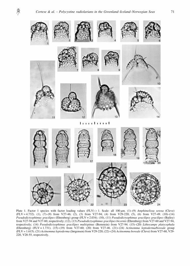
Plate 1. Factor 1 species with factor loading values (FLV) � 1. Scale: all 100 �m. (1)–(9) Amphimelissa setosa (Cleve)(FLV = 4.732). (1), (7)–(9) from V27-46; (2), (3) from V27-94; (4) from V29-220; (5), (6) from V27-49. (10)–(14)Pseudodictyophimus gracilipes (Ehrenberg) group (FLV = 2.034). (10), (11) Pseudodictyophimus gracilipes gracilipes (Bailey)from V27-94 and V27-60, respectively; (12), (13) Pseudodictyophimus gracilipes bicornis (Ehrenberg) from V27-60 and V27-94,respectively; (14) Pseudodictyophimus gracilipes multispinus (Bernstein) from V27-94. (15)–(20) Lithocampe platycephala(Ehrenberg) (FLV = 1.731). (15)–(19) from V27-60; (20) from V27-46. (21)–(24) Actinomma leptoderma/boreale group(FLV = 1.615). (21) Actinomma leptoderma (Jørgensen) from V29-220; (22)–(24) Actinomma boreale (Cleve) from V27-60, V29-220, V28-55, respectively.


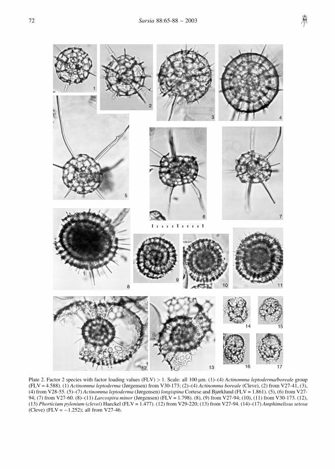
Plate 2. Factor 2 species with factor loading values (FLV) � 1. Scale: all 100 �m. (1)–(4) Actinomma leptoderma/boreale group(FLV = 4.588). (1) Actinomma leptoderma (Jørgensen) from V30-173; (2)–(4) Actinomma boreale (Cleve), (2) from V27-41, (3),(4) from V28-55. (5)–(7) Actinomma leptoderma (Jørgensen) longispina Cortese and Bjørklund (FLV = 1.861). (5), (6) from V27-94; (7) from V27-60. (8)–(11) Larcospira minor (Jørgensen) (FLV = 1.798). (8), (9) from V27-94; (10), (11) from V30-173. (12),(13) Phorticium pylonium (clevei) Haeckel (FLV = 1.477). (12) from V29-220; (13) from V27-94. (14)–(17) Amphimelissa setosa(Cleve) (FLV = �1.252); all from V27-46.

72 Sarsia 88:65-88 – 2003

Plate 3. Factor 3 species with factor loading values (FLV) � 1. Scale: all 100 �m, except (3). (1), (2) Larcospira minor (Jørgensen)(FLV = 3.421); both from V29-220. (3), (4) Spongotrochus glacialis group (FLV = 3.294). (3) Spongotrochus glacialis fromV28-55 (scale = 50 �m); (4) Spongodiscus osculosus from V28-55. (5) Phorticium pylonium clevei Haeckel (FLV = 1.956); fromV30-173. (6), (7), (10), (11) Actinomma leptoderma/boreale group (FLV = �1.661); (10) Actinomma leptoderma (Jørgensen) fromV30-173; (6), (7), (11) Actinomma boreale (Cleve), (7), (10) from V30-173, (11) from V27-60. (8), (9), (12) Actinomma sp. 2(FLV = 1.091); all from K23413. (13)–(15) Larcoidea sp. 1 (FLV = 1.086); (13) from V29-220; (14), (15) from V30-173.


Plate 4. Factor 4 species with factor loading values (FLV) � 1. Scale: all 100 �m. (1)–(7) Lithomelissa setosa Jørgensen(FLV = 3.683); (1), (2), (4), (7) from V27-94; (3) from V29-220; (5) from V30-173; (6) from V28-55. (8)–(11) Artobotrys borealis(Cleve) (FLV = 2.388); (8), (9) from V29-220; (10), (11) from V23-94. (12)–(15) Pseudodictyophimus gracilipes group(FLV = 1.577). (12) Pseudodictyophimus gracilipes bicornis (Ehrenberg) from V27-94; (13) Pseudodictyophimus gracilipesgracilipes (Bailey) from V27-94; (14), (15) Pseudodictyophimus gracilipes multispinus (Bernstein) from V27-60. (16), (17)Amphimelissa setosa (Cleve) (FLV = �1.310). (16) from V30-173; (17) from V27-60. (18), (19) Phorticium pylonium (clevei)Haeckel (FLV = 1.273); both from V30-173. (20)–(22) Lithomelissa hystrix Jørgensen (FLV = 1.124). (20) from V27-60; (21),(22) from V27-94. (23)–(26) Lithomitra lineata (Ehrenberg) (FLV = 1.217). (23), (24) from V27-60; (25) from V27-94; (26) fromV29-220. (27), (28) Corocalyptra craspedota Jørgensen (FLV = 1.036). (27) from V27-94; (28) from V29-219.

74 Sarsia 88:65-88 – 2003

Greenland Sea, and from August until October in theNorwegian Sea. Therefore, microfossils in the surfacesediments from the GIN Seas generally reflect thesummer/autumn production maximum in the surfacewater masses (Matthiessen & al. 2001).

The main surface currents and the bottom topographyof the study area are shown in Fig. 2.

Q-mode factor analysis (Imbrie & Kipp 1971) wasused for the statistical treatment of the data set, usingthe software packages PalaeoToolBox and Mac Trans-fer (Sieger & al. 1999).

Q-mode factor analysis can be described as a rotationof data points in multidimensional space, in order forthe longest axis (the one with the greatest variance) tobe the first factor axis, the second longest axis,perpendicular to the first, is the second factor axis,and so on. An eigenvector (a series of componentloadings for each taxon, indicating the relative impor-tance of each taxon in the extracted principal compo-nent) is associated with each of these component axes.The faunal assemblages and species relative abundancemaps have been produced by PanMap (Diepenbroek &al. 2000) and Arc View. The core-top data set has alsobeen examined by means of cluster analysis, using thesoftware package Past (Hammer & al. 2001), with anunweighted pair grouping method and a Spearmanrank-order correlation coefficient.

Many similarity indexes can be used as input forcluster analysis. The evaluation of the characteristics ofthe input data set can help in choosing an appropriatesimilarity index. When dealing with fossil data, whosedistribution can be affected by processes such as lateraltransport, differential dissolution, winnowing, rework-ing, non-metric, quantitative similarity measures (e.g.Spearman rank-order correlation coefficient) should beused (Sneath & Sokal 1973). One of the advantages of a

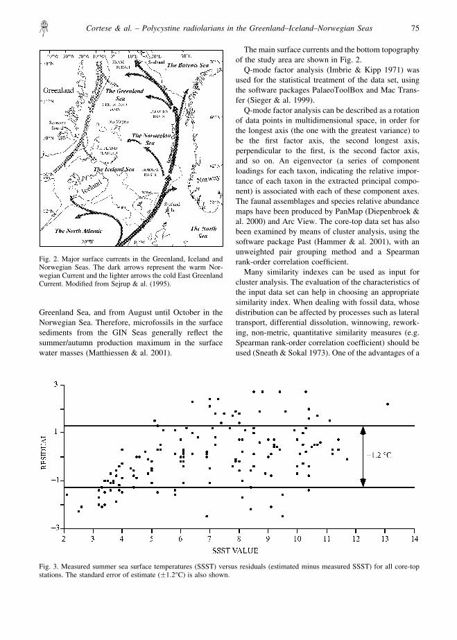
Fig. 2. Major surface currents in the Greenland, Iceland andNorwegian Seas. The dark arrows represent the warm Nor-wegian Current and the lighter arrows the cold East GreenlandCurrent. Modified from Sejrup & al. (1995).

Fig. 3. Measured summer sea surface temperatures (SSST) versus residuals (estimated minus measured SSST) for all core-topstations. The standard error of estimate (�1.2°C) is also shown.


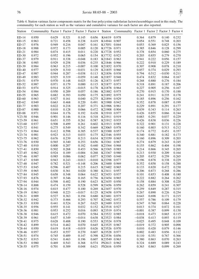
Table 4. Station varimax factor components matrix for the four polycystine radiolarian factors/assemblages used in this study. Thecommunality for each station as well as the variance and cumulative variance for each factor are also reported.

Station Communality Factor 1 Factor 2 Factor 3 Factor 4 Station Communality Factor 1 Factor 2 Factor 3 Factor 4

ED-14 0.950 0.629 0.321 0.145 0.656 K44/19 0.978 0.364 0.879 0.140 0.232ED-15 0.963 0.721 0.458 0.238 0.419 K14944 0.907 0.054 0.551 0.748 0.203ED-17 0.976 0.949 0.216 0.047 0.161 K17051 0.844 0.053 0.369 0.825 0.156ED-18 0.988 0.972 0.173 0.005 0.120 K17726 0.971 0.385 0.846 0.128 0.299ED-21 0.984 0.874 0.415 0.011 0.220 K17728 0.952 0.378 0.854 0.060 0.275ED-30 0.972 0.952 0.196 0.065 0.154 K17732 0.923 0.203 0.855 0.279 0.270ED-37 0.979 0.911 0.338 �0.048 0.183 K21843 0.963 0.941 0.222 0.056 0.157ED-38 0.985 0.929 0.258 0.036 0.235 K21846 0.966 0.222 0.910 0.229 0.189ED-39 0.984 0.963 0.215 �0.007 0.100 K21852 0.970 0.307 0.908 0.078 0.210ED-40 0.977 0.929 0.310 �0.031 0.129 K21855 0.960 0.857 0.374 0.029 0.293ED-47 0.987 0.944 0.287 �0.038 0.113 K21856 0.938 0.794 0.512 �0.030 0.211ED-49 0.983 0.925 0.319 �0.059 0.148 K21857 0.948 0.474 0.832 0.064 0.167ED-51 0.979 0.970 0.148 0.025 0.126 K21873 0.957 0.268 0.880 0.276 0.184ED-52 0.987 0.971 0.179 0.000 0.115 K21877 0.973 0.318 0.891 0.187 0.206ED-53 0.974 0.914 0.325 �0.015 0.178 K21878 0.964 0.227 0.905 0.256 0.167ED-54 0.984 0.950 0.209 0.057 0.186 K21882 0.975 0.270 0.915 0.170 0.188ED-55 0.965 0.882 0.393 0.050 0.175 K21892 0.975 0.241 0.911 0.235 0.178ED-60 0.963 0.927 0.161 0.040 0.275 K21894 0.929 0.185 0.896 0.256 0.162ED-62 0.949 0.663 0.468 0.220 0.491 K21900 0.942 0.352 0.878 0.087 0.199ED-77 0.903 0.822 0.218 0.207 0.371 K21906 0.961 0.229 0.891 0.291 0.177ED-87 0.900 0.810 0.128 0.066 0.472 K21908 0.904 0.839 0.343 0.114 0.263ED-88 0.971 0.844 0.176 0.192 0.438 K21910 0.977 0.426 0.855 0.066 0.244V23-58 0.946 0.901 0.146 0.116 0.318 K21911 0.919 0.883 0.291 0.037 0.229V23-59 0.961 0.651 0.355 0.261 0.587 K21912 0.935 0.426 0.838 0.036 0.226V23-60 0.937 0.508 0.499 0.261 0.602 K21913 0.985 0.322 0.901 0.131 0.228V23-72 0.941 0.275 0.549 0.342 0.669 K23065 0.978 0.160 0.803 0.513 0.212V23-73 0.964 0.412 0.598 0.385 0.537 K23300 0.957 0.174 0.772 0.451 0.357V23-74 0.981 0.923 0.313 0.033 0.175 K23346 0.955 0.340 0.881 0.182 0.173V23-75 0.962 0.676 0.239 0.213 0.634 K23359 0.965 0.160 0.896 0.309 0.203V23-76 0.930 0.565 0.340 0.253 0.656 K23361 0.967 0.274 0.879 0.243 0.245V27-40 0.910 0.800 0.207 0.182 0.440 K23364 0.968 0.155 0.862 0.404 0.198V27-41 0.850 0.502 0.268 0.453 0.566 K23365 0.985 0.214 0.866 0.345 0.265V27-45 0.962 0.924 0.189 �0.004 0.268 K23367 0.980 0.213 0.930 0.209 0.164V27-46 0.987 0.985 0.086 0.062 0.077 K23385 0.940 0.205 0.872 0.259 0.265V27-47 0.949 0.943 0.243 �0.013 �0.010 K23398 0.977 0.196 0.878 0.338 0.229V27-48 0.947 0.782 0.521 �0.148 0.206 K23400 0.969 0.352 0.858 0.158 0.288V27-53 0.945 0.596 0.407 0.215 0.615 K23402 0.965 0.133 0.820 0.472 0.230V27-59 0.965 0.830 0.361 0.020 0.380 K23411 0.957 0.206 0.873 0.268 0.286V27-84 0.945 0.658 0.348 0.064 0.622 K23453 0.937 0.101 0.853 0.408 0.180V27-93 0.876 0.397 0.346 0.165 0.756 K23454 0.965 0.222 0.882 0.264 0.262V27-94 0.944 0.598 0.402 0.190 0.623 K23455 0.950 0.158 0.884 0.308 0.220V28-14 0.888 0.474 0.159 0.528 0.599 K23456 0.959 0.262 0.859 0.241 0.307V28-16 0.974 0.815 0.477 0.100 0.269 K23457 0.970 0.259 0.849 0.287 0.315V28-19 0.963 0.948 0.223 �0.017 0.125 K23458 0.979 0.267 0.890 0.226 0.254V28-31 0.909 0.527 0.363 0.194 0.680 K23481 0.975 0.643 0.698 0.171 0.215V28-32 0.942 0.373 0.466 0.293 0.707 K23482 0.972 0.557 0.786 0.109 0.179V28-33 0.930 0.441 0.524 0.267 0.625 K23489 0.933 0.547 0.760 0.064 0.228V28-35 0.956 0.955 0.141 0.032 0.152 K23518 0.927 0.013 0.374 0.872 0.161V28-36 0.981 0.953 0.252 0.016 0.093 K23519 0.974 �0.001 0.387 0.899 0.130V28-38 0.946 0.615 0.472 0.070 0.584 K23522 0.985 �0.018 0.473 0.865 0.115V28-39 0.961 0.657 0.349 �0.014 0.638 K23523 0.984 �0.038 0.413 0.893 0.119V28-41 0.975 0.628 0.488 0.190 0.553 K23524 0.978 �0.025 0.495 0.848 0.109V28-42 0.899 0.514 0.462 0.070 0.645 K23525 0.967 �0.019 0.372 0.905 0.098V28-44 0.950 0.619 0.418 �0.019 0.626 K23526 0.970 0.010 0.420 0.879 0.146V28-46 0.957 0.453 0.557 0.270 0.607 K23528 0.977 0.002 0.483 0.856 0.112V28-51 0.974 0.745 0.489 0.147 0.398 K23536 0.856 0.110 0.351 0.767 0.366V28-52 0.915 0.541 0.463 0.196 0.607 K23549 0.963 0.380 0.863 0.070 0.263V28-53 0.980 0.469 0.543 0.368 0.574 PS2613 0.962 0.324 0.889 0.089 0.243V28-55 0.975 0.701 0.309 0.048 0.621 PS2616 0.959 0.363 0.863 0.099 0.269

76 Sarsia 88:65-88 – 2003

Spearman rank-order coefficient and the unweightedpairs clustering method is that they are not too muchaffected by large variations in species abundances andby the distribution of rarer taxa, and are thereforecommonly used in palaeo-ecology (Sneath & Sokal1973).

All data presented in this paper are available inelectronic format from the Pangaea databank at http://www.pangaea.de

RESULTS

FACTOR ANALYSIS

The first four factors (assemblages) explain 95.41% ofthe total information contained in the data set (Table 3),and we interpret them as representing distinct oceano-graphic, sedimentological and/or opal preservationprovinces. The temperature regression equation has astandard error of estimate of �1.2°C (Table 3, Fig. 3)and a multiple correlation coefficient of 0.88. Most ofthe residuals (actual minus estimated temperature valuefor all core-tops) are <2°C.

The resulting varimax factor components (Table 4)are plotted by stations in a set of maps (Figs 4–7) tofacilitate the geographical interpretation of theextracted factors.

We interpreted factor 1 (Fig. 4) as a cold (Polar andArctic) water factor, because high (�0.80) factorloadings are found on the Iceland Plateau. In the

southern portion of the study area (south of ca 70°N)factor loadings �0.40 are located on the Iceland Plateauand on the northern side of the Iceland–Faeroe Ridgeuntil about 2°E. Similar high values are also found inthe eastern part of the Greenland Sea in a southeast–northwest trending zone. Values higher than 0.50–0.60approximately trace the position of the Arctic Front andthe intrusion of the cold East Iceland Current towardsthe southern sector of the Norwegian Basin. Amphime-lissa setosa dominated this factor with a varimax factorscore of 4.732 (Table 3). Other important species infactor 1 are the Pseudodictyophimus gracilipes group(2.034) and Lithocampe platycephala (1.731).

Factor 2 (Fig. 5) was best described as a GreenlandSea factor, as loadings higher than 0.80 are to be foundalong a southwest–northeast trending belt going fromScoresby Sound on the eastern coast of Greenland to thewestern coast of Spitsbergen. We associate this patternwith the gyre where branches of cold and warm currentsmix to the north of Mohns Ridge and to the west ofKnipovich Ridge. Similar high values are also presentin the northern part of the Lofoten Basin, approximatelylocated over the Mohns Ridge. High absolute values(Table 3) of varimax scores (4.588) were obtained forthe Actinomma leptoderma/boreale group, Actinommaleptoderma longispina (1.861) and Larcospira minor(1.798). Bjørklund & al. (1998) observed that therelative abundances of Actinomma leptodermaincreased towards the ice-edge off Greenland. This

Station Communality Factor 1 Factor 2 Factor 3 Factor 4 Station Communality Factor 1 Factor 2 Factor 3 Factor 4

V28-56 0.956 0.689 0.467 0.118 0.500 PS2644 0.918 0.536 0.701 0.253 0.273V28-58 0.967 0.917 0.148 0.169 0.274 PS2645 0.970 0.537 0.776 0.228 0.165V28-59 0.967 0.823 0.335 0.080 0.414 V27-60 0.954 0.617 0.366 0.140 0.648V28-60 0.974 0.751 0.336 0.166 0.519 V27-63 0.967 0.520 0.448 0.169 0.684V28-60A 0.954 0.752 0.220 0.190 0.552 V27-69 0.950 0.732 0.413 0.095 0.484V29-208 0.944 0.859 0.155 0.118 0.409 V27-74 0.945 0.617 0.542 0.327 0.404V29-209 0.913 0.748 0.258 0.058 0.533 V27-75 0.941 0.733 0.466 0.196 0.385V29-210 0.945 0.802 0.289 0.198 0.423 V27-76 0.948 0.702 0.416 0.226 0.481V29-211 0.975 0.807 0.372 0.036 0.429 V27-80 0.934 0.681 0.479 0.238 0.430V29-219 0.964 0.671 0.392 0.119 0.588 V27-96 0.939 0.541 0.271 0.269 0.707V29-220 0.965 0.682 0.262 0.161 0.637 V28-17 0.953 0.828 0.445 0.052 0.259V30-125 0.879 0.127 0.470 0.686 0.414 V28-21 0.984 0.823 0.477 0.102 0.262V30-130 0.959 0.923 0.229 �0.028 0.234 V28-26 0.944 0.866 0.355 0.005 0.259V30-131 0.984 0.970 0.144 0.083 0.123 V28-48 0.965 0.587 0.493 0.226 0.572V30-132 0.973 0.833 0.284 0.285 0.344 V28-49 0.934 0.641 0.548 0.255 0.397V30-133 0.948 0.729 0.332 0.126 0.540 V30-163 0.898 0.387 0.524 0.188 0.662V30-135 0.978 0.932 0.284 0.048 0.160 V30-142 0.971 0.626 0.651 0.162 0.360V30-167 0.959 0.481 0.442 0.146 0.715 V30-143 0.920 0.728 0.375 0.269 0.421V30-169 0.928 0.443 0.556 0.216 0.613 V30-144 0.955 0.709 0.475 0.275 0.388V30-170 0.961 0.412 0.432 0.335 0.702V30-175 0.959 0.453 0.464 0.198 0.706 Variance 39.331 31.412 9.272 15.395HM31-35 0.943 0.656 0.401 0.107 0.584 Cum. variance 39.331 70.743 80.015 95.409K31/2 0.963 0.102 0.754 0.585 0.208

Table 4. Continued.


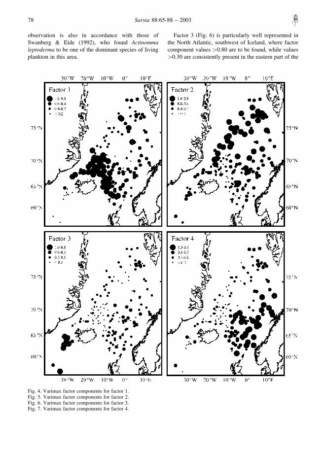
observation is also in accordance with those ofSwanberg & Eide (1992), who found Actinommaleptoderma to be one of the dominant species of livingplankton in this area.

Factor 3 (Fig. 6) is particularly well represented inthe North Atlantic, southwest of Iceland, where factorcomponent values �0.80 are to be found, while values�0.30 are consistently present in the eastern part of the

Fig. 4. Varimax factor components for factor 1.Fig. 5. Varimax factor components for factor 2.Fig. 6. Varimax factor components for factor 3.Fig. 7. Varimax factor components for factor 4.

78 Sarsia 88:65-88 – 2003

GIN Seas (Norway and Lofoten Basins and offSpitsbergen). These areas are under the influence ofwarm waters, as the Irminger current flows in the waterssouthwest of Iceland, and the Norwegian Current (thenorthward-bound branch of the Gulf Stream) flowsoffshore Norway in the eastern GIN Seas. Larcospira

minor (3.421), the Spongotrochus group (Spongotro-chus glacialis � Spongopyle osculosa � Spongodiscusresurgens) (3.294), and Phorticium pylonium (clevei)(1.956) were the species with the highest scaledvarimax factor scores (Table 3).

Factor 4 (Fig. 7) has been interpreted as a warm

Fig. 8. Relative abundance of Amphimelissa setosa in surface sediments.Fig. 9. Relative abundance of the Pseudodictyophimus gracilipes group in surface sediments.Fig. 10. Relative abundance of Lithocampe platycephala in surface sediments.Fig. 11. Relative abundance of the Actinomma leptoderma/boreale group in surface sediments.


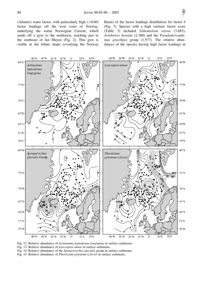
(Atlantic) water factor, with particularly high (�0.60)factor loadings off the west coast of Norway,underlying the warm Norwegian Current, whichsends off a gyre to the northwest, reaching just tothe southeast of Jan Mayen (Fig. 2). This gyre isvisible in the lobate shape (overlying the Norway

Basin) of the factor loadings distribution for factor 4(Fig. 7). Species with a high varimax factor score(Table 3) included Lithomelissa setosa (3.683),Artobotrys boreale (2.388) and the Pseudodictyophi-mus gracilipes group (1.577). The relative abun-dances of the species having high factor loadings in

Fig. 12. Relative abundance of Actinomma leptoderma longispina in surface sediments.Fig. 13. Relative abundance of Larcospira minor in surface sediments.Fig. 14. Relative abundance of the Spongotrochus glacialis group in surface sediments.Fig. 15. Relative abundance of Phorticium pylonium (clevei) in surface sediments.

80 Sarsia 88:65-88 – 2003

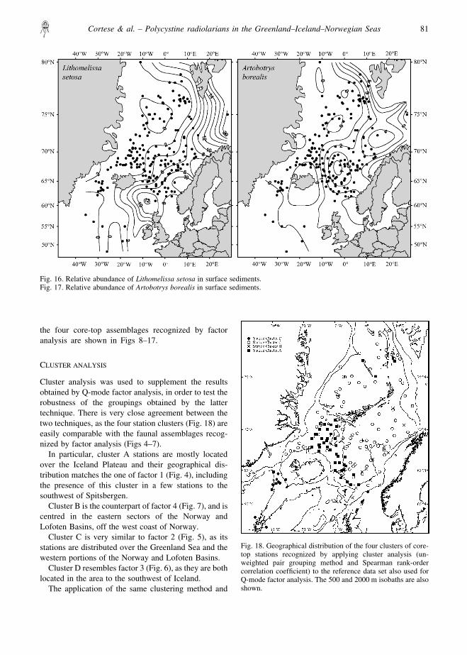
the four core-top assemblages recognized by factoranalysis are shown in Figs 8–17.

CLUSTER ANALYSIS

Cluster analysis was used to supplement the resultsobtained by Q-mode factor analysis, in order to test therobustness of the groupings obtained by the lattertechnique. There is very close agreement between thetwo techniques, as the four station clusters (Fig. 18) areeasily comparable with the faunal assemblages recog-nized by factor analysis (Figs 4–7).

In particular, cluster A stations are mostly locatedover the Iceland Plateau and their geographical dis-tribution matches the one of factor 1 (Fig. 4), includingthe presence of this cluster in a few stations to thesouthwest of Spitsbergen.

Cluster B is the counterpart of factor 4 (Fig. 7), and iscentred in the eastern sectors of the Norway andLofoten Basins, off the west coast of Norway.

Cluster C is very similar to factor 2 (Fig. 5), as itsstations are distributed over the Greenland Sea and thewestern portions of the Norway and Lofoten Basins.

Cluster D resembles factor 3 (Fig. 6), as they are bothlocated in the area to the southwest of Iceland.

The application of the same clustering method and

Fig. 16. Relative abundance of Lithomelissa setosa in surface sediments.Fig. 17. Relative abundance of Artobotrys borealis in surface sediments.

Fig. 18. Geographical distribution of the four clusters of core-top stations recognized by applying cluster analysis (un-weighted pair grouping method and Spearman rank-ordercorrelation coefficient) to the reference data set also used forQ-mode factor analysis. The 500 and 2000 m isobaths are alsoshown.


similarity index to the transposed data matrix (Fig. 19)yields results which are comparable with what wewould have obtained by R-mode factor analysis (i.e.which species are important in which station cluster/area).

We have labelled the four main clusters according totheir geographical interpretation (Fig. 19), resulting in(from top to bottom):

� A Greenland Sea species cluster, including Larco-spira minor, Phorticium pylonium (clevei), Strebla-cantha circumtexta, Actinomma leptodermalongispina and the Actinomma leptoderma/borealegroup, corresponding to station cluster C;

� An Iceland Plateau species cluster, including Amphi-melissa setosa and Sethoconus tabulatus, correspond-ing to station cluster A;

� A Norwegian Sea species cluster, including Actinom-ma sp. 1, Plagiacantha arachnoides, Artobotrysborealis, Lithomitra lineata, Artostrobus joergenseni,the Pseudodictyophimus gracilipes group, Tholo-spyris gephyristes, Lithocampe platycephala, Plecta-cantha oikiskos, Ceratocyrtis galeus, Ceratocyrtishistricosus, Lipmanella xiphephorum, Corocalyptracraspedota, Lithomelissa setosa, Lithomelissahystrix, Lithomelissa thoracites, Lithomelissa sp.aff. L. stigi, corresponding to station cluster B;

� A North Atlantic species cluster, including Actinom-ma medianum, Actinomma sp. 2, the Spongotrochusglacialis group, Eucyrtidium calvertense, Phorticiumsp. 1, Stylatractus sp. 1, the drift fauna (Spongocorepuella, Theocorythium trachelium, Lamprocyclasmaritalis and Euchitonia spp.), Larcoidea sp. 1,Lithelius spiralis, Streblacantha sp. 1, correspondingto station cluster D.

NUMBER OF POLYCYSTINE RADIOLARIANS PER GRAMBULK SEDIMENT

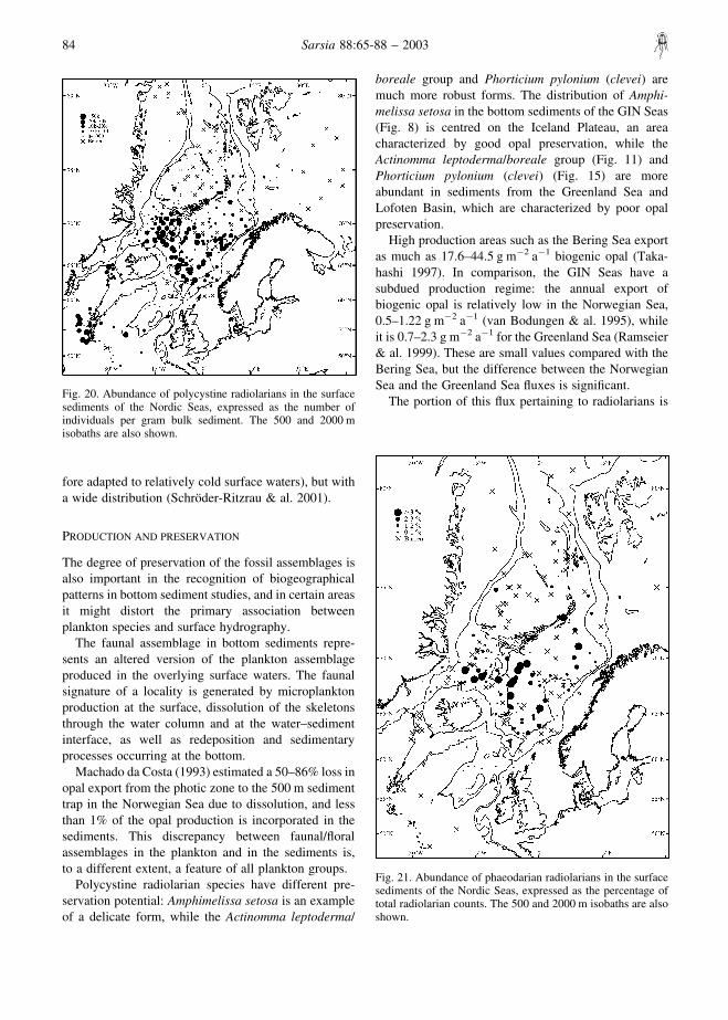
The geographical distribution of the number of poly-cystine radiolarians per gram bulk sediment (Fig. 20)can give indications on a variety of processes, such asthe production of radiolarians in the water column,export efficiency of their skeletons to the sediment,chemical dissolution/terrigenous dilution mechanismsat the seafloor. In order to separate between theseprocesses, additional information is necessary (seeDiscussion).

In the study area, abundant (generally more than10,000) radiolarian skeletons per gram bulk sedimentare found in the North Atlantic, to the southwest ofIceland, on the Iceland Plateau, and in the NorwegianSea. Intermediate values (generally less than 1000) are

found in the Lofoten Basin, with higher values along theflow pattern of the Norwegian Current (Fig. 2). Lowvalues (barren to less than 1000) are reported from theGreenland Basin, the Barents Sea, as well as from theslope off Scoresby Sound (Greenland).

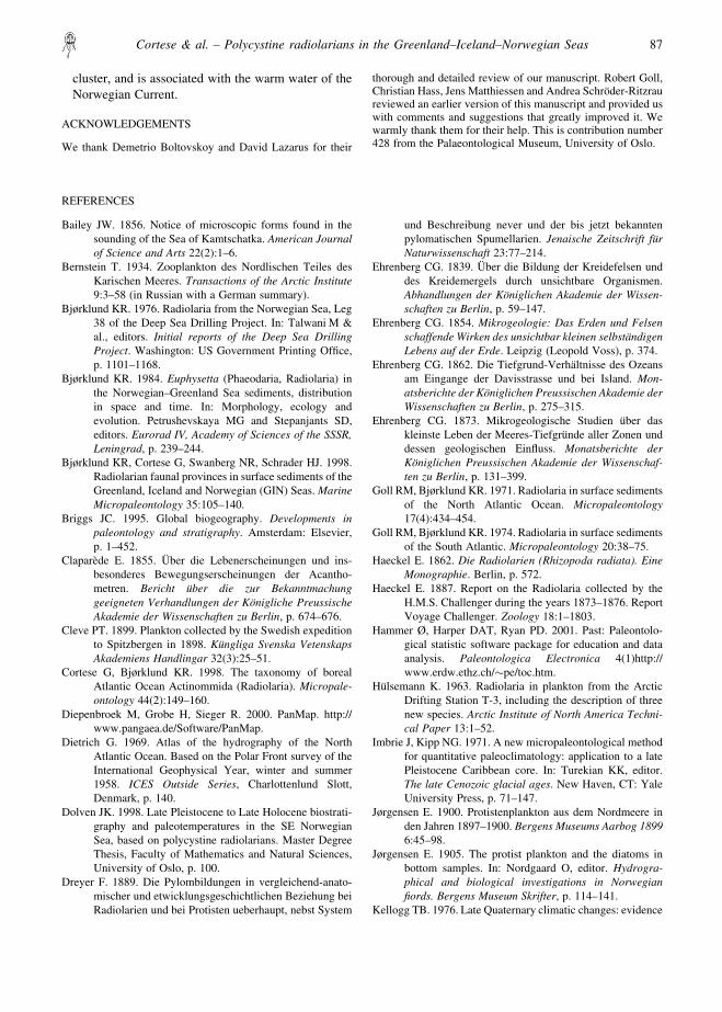
PHAEODARIA RELATIVE ABUNDANCE

The pattern of Phaeodaria relative abundance (Fig. 21)can provide insights into existing preservation/dissolu-tion provinces (see Discussion), as their skeleton ismore unstable (containing less opaline silica) andtherefore more easily dissolved than polycystine radio-larians.

The geographical distribution of Phaeodaria in thesediment (Fig. 21) of the GIN Seas is approximatelyequivalent to the one for the number of radiolarians pergram bulk sediment (Fig. 20). In fact, abundanceshigher than 1% are almost exclusively found on theIceland Plateau, in the Norwegian Sea, and in theLofoten Basin (limited to the area influenced by theNorwegian Current). Moreover, Phaeodaria are vir-tually absent in the sediments from the Greenland Sea,the Barents Sea, and off Scoresby Sound. The twoabundance patterns diverge significantly in both theNorth Atlantic southwest of Iceland, and on the VøringPlateau, where the absence of Phaeodaria in thesediment is not matched by the relatively abundantnumber of radiolarians per gram bulk sediment.

DISCUSSION

TEMPERATURE

The Norwegian Sea is mostly influenced by warm waterfrom the North Atlantic, while the Greenland Sea andthe Iceland Plateau are under the influence of cold Polarand Arctic waters. It is therefore to be expected, asstated by Briggs (1995), that temperature is the mostimportant ecological factor in determining the globaldistribution, or biogeography, of plankton (in this caseradiolarian species) in the surface waters, which is alsotraceable in the distribution pattern of radiolarianskeletons in the bottom sediments.

As an example, in the GIN Seas, we find Lithomelissasetosa and Larcospira sp. 1 to be more abundant insediments underlying warm water (Norway Basin),while the Actinomma leptoderma/boreale group andAmphimelissa setosa are most abundantly found insediments underlying cold waters (in the Greenland Seaand the Iceland Plateau, respectively). Other taxa, likeArtobotrys borealis, Lithomitra lineata and the P.gracilipes group, are interpreted as Arctic (and there-

82 Sarsia 88:65-88 – 2003

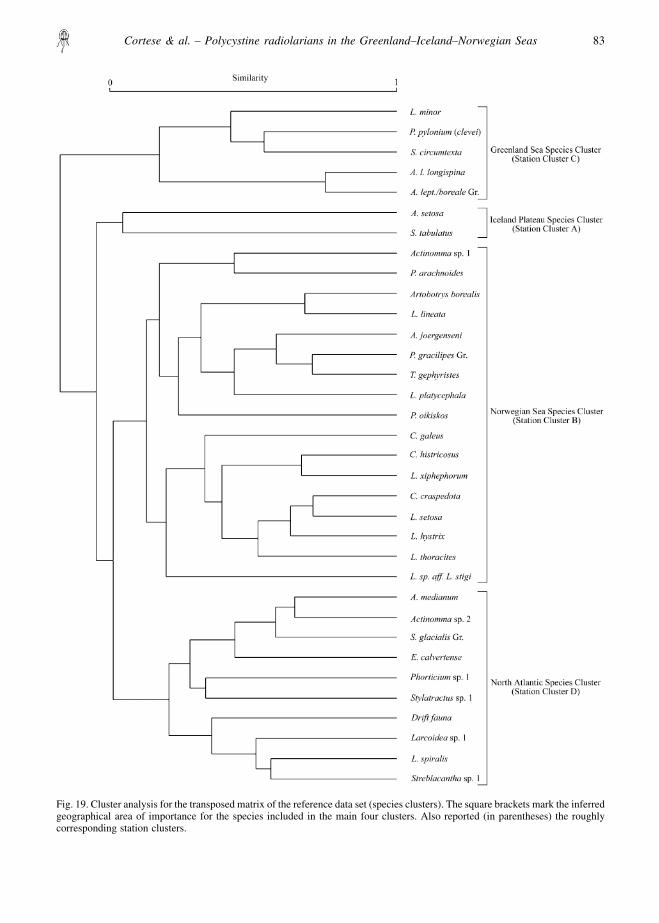
Fig. 19. Cluster analysis for the transposed matrix of the reference data set (species clusters). The square brackets mark the inferredgeographical area of importance for the species included in the main four clusters. Also reported (in parentheses) the roughlycorresponding station clusters.


fore adapted to relatively cold surface waters), but witha wide distribution (Schroder-Ritzrau & al. 2001).

PRODUCTION AND PRESERVATION

The degree of preservation of the fossil assemblages isalso important in the recognition of biogeographicalpatterns in bottom sediment studies, and in certain areasit might distort the primary association betweenplankton species and surface hydrography.

The faunal assemblage in bottom sediments repre-sents an altered version of the plankton assemblageproduced in the overlying surface waters. The faunalsignature of a locality is generated by microplanktonproduction at the surface, dissolution of the skeletonsthrough the water column and at the water–sedimentinterface, as well as redeposition and sedimentaryprocesses occurring at the bottom.

Machado da Costa (1993) estimated a 50–86% loss inopal export from the photic zone to the 500 m sedimenttrap in the Norwegian Sea due to dissolution, and lessthan 1% of the opal production is incorporated in thesediments. This discrepancy between faunal/floralassemblages in the plankton and in the sediments is,to a different extent, a feature of all plankton groups.

Polycystine radiolarian species have different pre-servation potential: Amphimelissa setosa is an exampleof a delicate form, while the Actinomma leptoderma/

boreale group and Phorticium pylonium (clevei) aremuch more robust forms. The distribution of Amphi-melissa setosa in the bottom sediments of the GIN Seas(Fig. 8) is centred on the Iceland Plateau, an areacharacterized by good opal preservation, while theActinomma leptoderma/boreale group (Fig. 11) andPhorticium pylonium (clevei) (Fig. 15) are moreabundant in sediments from the Greenland Sea andLofoten Basin, which are characterized by poor opalpreservation.

High production areas such as the Bering Sea exportas much as 17.6–44.5 g m�2 a�1 biogenic opal (Taka-hashi 1997). In comparison, the GIN Seas have asubdued production regime: the annual export ofbiogenic opal is relatively low in the Norwegian Sea,0.5–1.22 g m�2 a�1 (van Bodungen & al. 1995), whileit is 0.7–2.3 g m�2 a�1 for the Greenland Sea (Ramseier& al. 1999). These are small values compared with theBering Sea, but the difference between the NorwegianSea and the Greenland Sea fluxes is significant.

The portion of this flux pertaining to radiolarians isFig. 20. Abundance of polycystine radiolarians in the surfacesediments of the Nordic Seas, expressed as the number ofindividuals per gram bulk sediment. The 500 and 2000 misobaths are also shown.

Fig. 21. Abundance of phaeodarian radiolarians in the surfacesediments of the Nordic Seas, expressed as the percentage oftotal radiolarian counts. The 500 and 2000 m isobaths are alsoshown.

84 Sarsia 88:65-88 – 2003

estimated via sediment trap studies. Schroder-Ritzrau &al. (2001) observed that the radiolarian flux in theGreenland Sea was ca 2.7 � 10�3 individuals m�2

day�1, while in the Norwegian Sea the flux was reducedto ca 1 � 10�3 individuals m�2 day�1.

The higher opal (and radiolarian) fluxes in the Polarand Arctic waters, than in the Norwegian Sea, are notreflected in the surface sediments (Schroder-Ritzrau &al. 2001). Matthiessen & al. (2001) therefore concludedthat preservation limits the applicability of siliceoussediment assemblages in regions which are influencedby cold surface waters, in this case the Greenland Sea.

However, Kohly (1998) observed that even if themain flux species of diatoms and radiolarians are notpreserved in the sediments, the heavily silicified post-bloom diatom species are dominant members of deepsediment traps and sediment assemblages.

Radiolarian sediment trap data support the occur-rence of strong dissolution in the Greenland Sea:Schroder-Ritzrau & al. (2001) report that the assem-blage of polycystine radiolarians in the water column isdominated, in the Greenland Sea, by Amphimelissasetosa, with up to 88% of the cumulative flux (37–56%in the Jan Mayen Current). In the sediments, accordingto our data, the abundance of this species drops to wellbelow 30% in most of the Greenland Sea, and neverexceeds 76% in the bottom sediment samples at anylocation in the GIN Seas. Therefore, our data are inaccordance with the observation that Amphimelissasetosa, the most dominant species in the plankton, doesnot survive the settling time through the water or theexposure time at the sediment/water interface, and ismostly dissolved before being incorporated in thesediment (Schroder-Ritzrau & al. 2001).

Our data also indicate that the actinommids (theActinomma leptoderma/boreale group) and larcoids(Phorticium pylonium (clevei), Larcospira minor) arealso strongly enriched in the Greenland Sea sediments(14.4 and 40.9%, respectively), compared with theplankton assemblages, where they are both present with1.3% [average of sediment trap OG 3 and OG 5 datafrom Schroder-Ritzrau (1995)].

In the specific case of radiolarians from the GINSeas, we believe that the small portion of producedbiogenic opal that is incorporated in the sediment stillkeeps primary information about the surface waterswhere radiolarians used to live before settling throughthe water column and being incorporated in thesediment. This is also indirectly demonstrated by thefact that our temperature regression equation (Table 3)has a high multiple correlation coefficient (0.88) and alow standard error of estimate (�1.2°C).

In contrast to the “poor opal preservation” Greenland

Sea, the Norwegian and Iceland Seas are exceptional inpreserving phaeodarian skeletons (Stadum & Ling1969; Bjørklund 1984). These skeletons are constructedof amorphous silica with traces of magnesium, calciumand copper (Reschetnyak 1966), and with an organiccompound or matrix that is poorly understood (Kling &Boltovskoy 1999). Finally, the spines are hollow andsome species have a bubbly, very sensitive to dissolu-tion, “styrofoam” structured skeleton. In Fig. 21 wehave plotted the percentage values of phaeodarianskeletons in the sediment. They are essentially notpreserved on the western side of the mid-oceanic ridgesystem, confirming that dissolution is quite active in theGreenland Sea (Schroder-Ritzrau & al. 2001).

Another main difference between the western andeastern GIN Seas consists in the fact that the GreenlandSea includes a sea–ice zone and a marginal ice zone,both characterized by highly stratified water masses anda strong haline stratification, while the adjacent opensea is not influenced by melt water and therefore notstratified.

The number of polycystine radiolarian specimens pergram bulk sediment (Fig. 20) can be used to defineoceanic/sedimentary provinces in the GIN Seas, pro-vided that this information is integrated with a generalknowledge of processes such as sediment transport andsources, productivity regimes, and surface currents inthis region.

In fact, areas with low radiolarian numbers in bottomsediments are usually associated with clear signs ofdissolution of opal microfossils (Goll & Bjørklund1971). Poor preservation of radiolarian skeletons in theGIN Seas is a widespread phenomenon: Bjørklund(unpublished data) observed poorly preserved speci-mens even from high abundance areas on the IcelandPlateau. Specimens of Lithocampe platycephala andAmphimelissa setosa had dissolution pits on the surfaceof the skeleton. These pits extended inwards, giving analmost hollow or tube-like appearance to the skeleton.This seems to take place all over the investigated area,but more so in the radiolarian low abundance areas. Wenotice, for example, that there is an enrichment ofspecies with heavily silicified skeletons, interpreted byus to be dissolution resistant species (the Actinommaleptoderma/boreale group, Phorticium pylonium (cle-vei), Larcospira minor, the Spongotrochus glacialisgroup) in station clusters C and D, Greenland Sea/northwestern Lofoten Basin and North Atlantic, respec-tively (Fig. 18), and by the disappearance, in the bottomsediments of the Greenland Sea, of Amphimelissasetosa and Plectacantha oikiskos, two species whichare reported to be common in the plankton at the ice-edge in the Greenland Sea (Swanberg & Eide 1992).


The distribution of both station clusters (Fig. 18) andradiolarian abundances (Fig. 20) can help to evaluatethe influence of preservational processes, bottomtopography, and radiolarian production in the studyarea.

CLUSTER ANALYSIS

Cluster A occupies the Norway Basin and the IcelandPlateau, bordered by the Iceland–Faeroe Ridge to thesouth, the Jan Mayen Fracture Zone to the north, theIceland–Jan Mayen Ridge to the west, and by the1500 m isobath to the east. Higher than averageabundance values in the Iceland Plateau and in theNorway Basin (values �50,000 radiolarians g�1 areexclusively found in these areas, Fig. 20) are an effectof high production and effective screening of ice-raftedmaterial from the west. This cluster can be roughlyseparated, along the 7°W meridian, in a “shallow andcold” Iceland Plateau cluster to the west, and a “deepand warm” Norway Basin cluster to the east.

Cluster B is located along the western coast ofNorway, i.e. in the eastern part of the Norway andLofoten Basins. Radiolarian abundances are higher inthe southern part of this cluster and decrease northwards(Fig. 20). This cluster crosses several bathymetricfeatures (Norway and Lofoten Basins, separated bythe Jan Mayen Fracture Zone and the Vøring Plateau)and seems to depict the path of the warm NorwegianCurrent. We therefore assume that primary productionis the most important influence on radiolarian abun-dances in the southern end of cluster B, whileterrigenous input and/or bathymetry are most importantin the northern end. The high terrigenous input and thefrequently observed turbidites in sediment cores in theLofoten Basin (Kellogg 1976) support this statement.

Cluster C is generally found west of the mid-AtlanticRidge, in the Lofoten Basin, and in the deepest part ofthe Norway Basin. The low radiolarian abundanceswest of the ridge (Greenland and Boreas Basins) aremost likely caused by low production (compared with,for example, the Bering Sea), input of terrigenousmaterial from the west by ice-rafting, while in theLofoten Basin slumping from the continental slopecould be the dominating process. Additionally bothareas are exposed to active opal dissolution, both in thewater column and at the sediment/water interface. In theGreenland Sea, cluster C is aligned on a southwest–northeast trending belt, whose western boundaryclosely resembles the summer ice-edge position.

The close relationship between cluster C, lowradiolarian abundances and high minerogenic inputseems to be confirmed by the fact that stations having

few radiolarians (barren to less than 1000 radiolariansg�1) are located in shallow areas, such as the North Sea,the Barents Sea and along the east coast of Greenland(Fig. 20). Barren stations are also found at depth in theLofoten, Greenland and Boreas Basins.

Cluster D is found in the North Atlantic, on theReykyanes Ridge. Even if the number of radiolarians ishigh in this area, the opal refractive index is high too, atypical feature of dissolved assemblages (Goll &Bjørklund 1971). This is also in harmony with thelow number of Phaeodaria (Fig. 21), another indicatorof poor preservation, found in sediment samples fromthis area.

CONCLUSIONS

� A regression equation for summer sea surfacetemperature has been developed for the GIN Seas,based on a reference core-top database including 160stations. The standard error of estimate for thisequation is �1.2°C. This provides an excellent toolfor radiolarian-based palaeotemperature estimates inthe GIN Seas.

� The distribution of radiolarian species and faunalassemblages in the surface sediments of the Green-land Sea allowed dissolution to be recognized as animportant factor in modifying the faunal signalgenerated in the plankton, without, however, hinder-ing the reliability of the temperature regressionequation (multiple correlation coefficient = 0.88 anda standard error of estimate = �1.2°C).

� Cluster analysis has been applied to the same data setand the results compared with those obtained byfactor analysis, the distribution of species relativeabundances, prevailing current systems, and preser-vation provinces in the GIN Seas. This allowed fourdifferent factors/assemblages/clusters to be recog-nized characterizing the different sub-basins in thestudy area.

� Factor 1 has a very similar distribution to the IcelandPlateau species cluster (station cluster A), and weinterpret it as a cold (Polar and Arctic) water factor.

� Factor 2 has a very similar distribution to theGreenland Sea species cluster (station cluster C),and is associated with the gyre formed by the JanMayen Current and the Norwegian Current, wherecold and warm waters mix.

� Factor 3 has a very similar distribution to the NorthAtlantic species cluster (station cluster D), associatedwith the warm Irminger Current southwest of Iceland.

� Factor 4 has a very similar distribution to theNorwegian Sea (Norway and Lofoten Basins) species

86 Sarsia 88:65-88 – 2003

cluster, and is associated with the warm water of theNorwegian Current.

ACKNOWLEDGEMENTS

We thank Demetrio Boltovskoy and David Lazarus for their

thorough and detailed review of our manuscript. Robert Goll,Christian Hass, Jens Matthiessen and Andrea Schroder-Ritzraureviewed an earlier version of this manuscript and provided uswith comments and suggestions that greatly improved it. Wewarmly thank them for their help. This is contribution number428 from the Palaeontological Museum, University of Oslo.

REFERENCES

Bailey JW. 1856. Notice of microscopic forms found in thesounding of the Sea of Kamtschatka. American Journalof Science and Arts 22(2):1–6.

Bernstein T. 1934. Zooplankton des Nordlischen Teiles desKarischen Meeres. Transactions of the Arctic Institute9:3–58 (in Russian with a German summary).

Bjørklund KR. 1976. Radiolaria from the Norwegian Sea, Leg38 of the Deep Sea Drilling Project. In: Talwani M &al., editors. Initial reports of the Deep Sea DrillingProject. Washington: US Government Printing Office,p. 1101–1168.

Bjørklund KR. 1984. Euphysetta (Phaeodaria, Radiolaria) inthe Norwegian–Greenland Sea sediments, distributionin space and time. In: Morphology, ecology andevolution. Petrushevskaya MG and Stepanjants SD,editors. Eurorad IV, Academy of Sciences of the SSSR,Leningrad, p. 239–244.

Bjørklund KR, Cortese G, Swanberg NR, Schrader HJ. 1998.Radiolarian faunal provinces in surface sediments of theGreenland, Iceland and Norwegian (GIN) Seas. MarineMicropaleontology 35:105–140.

Briggs JC. 1995. Global biogeography. Developments inpaleontology and stratigraphy. Amsterdam: Elsevier,p. 1–452.

Claparede E. 1855. Uber die Lebenerscheinungen und ins-besonderes Bewegungserscheinungen der Acantho-metren. Bericht uber die zur Bekanntmachunggeeigneten Verhandlungen der Konigliche PreussischeAkademie der Wissenschaften zu Berlin, p. 674–676.

Cleve PT. 1899. Plankton collected by the Swedish expeditionto Spitzbergen in 1898. Kungliga Svenska VetenskapsAkademiens Handlingar 32(3):25–51.

Cortese G, Bjørklund KR. 1998. The taxonomy of borealAtlantic Ocean Actinommida (Radiolaria). Micropale-ontology 44(2):149–160.

Diepenbroek M, Grobe H, Sieger R. 2000. PanMap. http://www.pangaea.de/Software/PanMap.

Dietrich G. 1969. Atlas of the hydrography of the NorthAtlantic Ocean. Based on the Polar Front survey of theInternational Geophysical Year, winter and summer1958. ICES Outside Series, Charlottenlund Slott,Denmark, p. 140.

Dolven JK. 1998. Late Pleistocene to Late Holocene biostrati-graphy and paleotemperatures in the SE NorwegianSea, based on polycystine radiolarians. Master DegreeThesis, Faculty of Mathematics and Natural Sciences,University of Oslo, p. 100.

Dreyer F. 1889. Die Pylombildungen in vergleichend-anato-mischer und etwicklungsgeschichtlichen Beziehung beiRadiolarien und bei Protisten ueberhaupt, nebst System

und Beschreibung never und der bis jetzt bekanntenpylomatischen Spumellarien. Jenaische Zeitschrift furNaturwissenschaft 23:77–214.

Ehrenberg CG. 1839. Uber die Bildung der Kreidefelsen unddes Kreidemergels durch unsichtbare Organismen.Abhandlungen der Koniglichen Akademie der Wissen-schaften zu Berlin, p. 59–147.

Ehrenberg CG. 1854. Mikrogeologie: Das Erden und Felsenschaffende Wirken des unsichtbar kleinen selbstandigenLebens auf der Erde. Leipzig (Leopold Voss), p. 374.

Ehrenberg CG. 1862. Die Tiefgrund-Verhaltnisse des Ozeansam Eingange der Davisstrasse und bei Island. Mon-atsberichte der Koniglichen Preussischen Akademie derWissenschaften zu Berlin, p. 275–315.

Ehrenberg CG. 1873. Mikrogeologische Studien uber daskleinste Leben der Meeres-Tiefgrunde aller Zonen unddessen geologischen Einfluss. Monatsberichte derKoniglichen Preussischen Akademie der Wissenschaf-ten zu Berlin, p. 131–399.

Goll RM, Bjørklund KR. 1971. Radiolaria in surface sedimentsof the North Atlantic Ocean. Micropaleontology17(4):434–454.

Goll RM, Bjørklund KR. 1974. Radiolaria in surface sedimentsof the South Atlantic. Micropaleontology 20:38–75.

Haeckel E. 1862. Die Radiolarien (Rhizopoda radiata). EineMonographie. Berlin, p. 572.

Haeckel E. 1887. Report on the Radiolaria collected by theH.M.S. Challenger during the years 1873–1876. ReportVoyage Challenger. Zoology 18:1–1803.

Hammer Ø, Harper DAT, Ryan PD. 2001. Past: Paleontolo-gical statistic software package for education and dataanalysis. Paleontologica Electronica 4(1)http://www.erdw.ethz.ch/�pe/toc.htm.

Hulsemann K. 1963. Radiolaria in plankton from the ArcticDrifting Station T-3, including the description of threenew species. Arctic Institute of North America Techni-cal Paper 13:1–52.

Imbrie J, Kipp NG. 1971. A new micropaleontological methodfor quantitative paleoclimatology: application to a latePleistocene Caribbean core. In: Turekian KK, editor.The late Cenozoic glacial ages. New Haven, CT: YaleUniversity Press, p. 71–147.

Jørgensen E. 1900. Protistenplankton aus dem Nordmeere inden Jahren 1897–1900. Bergens Museums Aarbog 18996:45–98.

Jørgensen E. 1905. The protist plankton and the diatoms inbottom samples. In: Nordgaard O, editor. Hydrogra-phical and biological investigations in Norwegianfiords. Bergens Museum Skrifter, p. 114–141.

Kellogg TB. 1976. Late Quaternary climatic changes: evidence


from deep-sea cores of Norwegian and Greenland Seas.Geological Society of America Memoir 145:77–110.

Kling SA, Boltovskoy D. 1999. Radiolaria Phaeodaria. In:Boltovskoy D, editor. South Atlantic zooplankton.Leiden: Backhuys, p. 213–264.

Koc N, Jansen E, Haflidason H. 1993. Paleoceanographicreconstructions of surface ocean conditions in theGreenland, Iceland and Norwegian seas through thelast 14 ka based on diatoms. Quaternary ScienceReview 12:115–140.

Koc N, Jansen E, Hald M, Labeyrie L. 1996. Late glacial-Holocene sea surface temperatures and gradientsbetween the North Atlantic and the Norwegian Sea:implications for the Nordic heat pump. GeologicalSociety Special Publication 111:177–185.

Koc-Karpuz N, Schrader H. 1990. Surface sediment diatomdistribution and Holocene paleotemperature variationsin the Greenland, Iceland and Norwegian seas. Pale-oceanography 5:557–580.

Kohly A. 1998. Diatom flux and species composition in theGreenland Sea and the Norwegian Sea in 1991–1992.Marine Geology 145(3–4):293–312.

Machado da Costa E. 1993. Production, sedimentation anddissolution of biogenic silica in the northern NorthAtlantic. PhD Thesis, University of Kiel, p. 123.

Martin GC. 1904. Radiolaria. In: Clark WB, Eastman CR,Glenn LC, Bagg RM, Bassler RS, Boyer CS, Case EC,Hollick CA, editors. Systematic paleontology of theMiocene deposits of Maryland: Baltimore. Baltimore:Maryland Geological Survey, Johns Hopkins Press, p.447–459.

Matthiessen J, Baumann K-H, Schroder-Ritzrau A, Hass C,Andruleit H, Baumann A, Jensen S, Kohly A, Pflau-mann U, Samtleben C, Schafer P, Thiede J. 2001.Distribution of calcareous, siliceous and organic-walledplanktic microfossils in surface sediments of the NordicSeas and their relation to surface-water masses. In:Schafer P, Ritzrau W, Schluter M, Thiede J, editors. Thenorthern North Atlantic: a changing environment.Berlin: Springer, p. 105–127.

Nigrini C. 1967. Radiolaria in pelagic sediments from theIndian and Atlantic Oceans. Bulletin of the ScrippsInstitution of Oceanography 11:1–125.

Peinert R, Bauerfeind E, Gradinger R, Haupt O, Krumbholz M,Peeken I, Werner I, Zeitzschel B. 2001. Biogenicparticle sources and vertical flux patterns in theseasonally ice-covered Greenland Sea. In: Schafer P,Ritzrau W, Schluter M, Thiede J, editors. The northernNorth Atlantic: a changing environment. Berlin:Springer, p. 69–79.

Petrushevskaya MG. 1969. Raspredelenie skeletov radioljarij vosadkah severiej Atlantiki. In: Vyalov OS, editor.Iskopaemye i sovrennye radioljarij. (Material vtorogovsesojoenogo seminara po radioljarijam). Vov: Uni-versity Press, p. 123–132.

Popofsky A. 1908. Die Radiolarien der Antarktis. DeutscheZoologische Sudpolar Expedition (1901–1903) 10:185–308.

Ramseier RO, Garrity C, Bauerfeind E, Peinert R. 1999. Sea-ice impact on long-term particle flux in the GreenlandSea’s Is Odden-Nordbukta region during 1985–1996.Journal of Geophysical Research 104:5329–5343.

Reschetnyak VV. 1966. Deep sea phaeodarian radiolaria of theNorthwest Pacific. Fauna SSSR, New Series 94:1–208.

Samtleben C, Schafer P, Andruleit H, Baumann A, BaumannKH, Kohly A, Matthiessen J, Schroder-Ritzrau A. 1995.Plankton in the Norwegian–Greenland Sea: from livingcommunities to sediment assemblages—an actualisticapproach. Geologische Rundschau 84:108–136.

Schroder-Ritzrau A. 1995. Aktuopalaontologische Unter-suchung zu Verbreitung und Verticalflux von Radio-larien sowie ihre raumliche und zeitliche Entwicklungim Europaischen Nordmeer. Berichte aus dem Sonder-forschungsbereich 313, Kiel University 52:1–99.

Schroder-Ritzrau A, Andruleit H, Jensen S, Samtleben C,Schafer P, Matthiessen J, Hass HC, Kohly A, Thiede J.2001. Distribution, export and alteration of fossilizableplankton in the Nordic Seas. In: Schafer P, Ritzrau W,Schluter M, Thiede J, editors. The northern NorthAtlantic: a changing environment. Berlin: Springer, p.81–104.

Sejrup HP, Haflidason H, Kristensen DK. 1995. Rapid Com-munication. Last interglacial and Holocene climaticdevelopment in the Norwegian Sea region: ocean frontmovements and ice-core data. Journal of QuaternaryScience 10(4):385–390.

Sieger R, Gersonde R, Zielinski U. 1999. A new extendedsoftware package for quantitative paleoenvironmentalreconstructions. EOS, Transactions, American Geo-physical Union, p. Electronic supplement.

Sneath PHA, Sokal RR. 1973. Numerical taxonomy: the prin-ciples and practice of numerical classification. SanFrancisco: Freeman, p. 573.

Stadum CJ, Ling HY. 1969. Tripylean radiolaria in deep-seasediments of the Norwegian Sea. Micropaleontology15:481–489.

Swanberg NR, Eide LK. 1992. The radiolarian fauna at the iceedge in the Greenland Sea during summer, 1988.Journal of Marine Research 50:297–320.

Takahashi K. 1997. Time-series fluxes of Radiolaria in theeastern subarctic Pacific Ocean. News of Osaka Micro-paleontologists, Special Volume 10:299–309.

van Bodungen B, Anita A, Bauerfeind E, Haupt O, Peeken I,Peinert R, Reitmeier S, Thomsen C, Voss M, WunschM, Zeller U, Zeitzschel B. 1995. Pelagic processes andvertical flux of particles: an overview over long-termcomparative study in the Norwegian Sea and GreenlandSea. Geologische Rundschau 84:11–27.

Accepted 21 January 2002 – Printed 24 April 2003Editorial responsibility: Jarl Giske

88 Sarsia 88:65-88 – 2003

giuseppe cortese, kjell r. bjørklund & jane k. dolven ... · koc¸-karpuz & schrader...

Documents