ghassan a. chammas portfolio concentration...will learn, for example, that in portfolio no.1 he is...
TRANSCRIPT

GHASSAN A. CHAMMAS
Portfolio Concentration


PORTFOLIO CONCENTRATION


PORTFOLIO CONCENTRATION
HET CONCENTRATIE NIVEAU VAN PORTEFEUILLES
Thesis
to obtain the degree of Doctor from the
Erasmus University Rotterdam
by command of the
Rector Magnificus
Prof.dr. H.A.P. POLS
and in accordance with the decision of the Doctorate Board.
The public defense shall be held on
Thursday, 26 January 2017 at 09:30 hours
by
GHASSAN AFIF CHAMMAS
born in AMIOUN, LEBANON

Doctoral Committee
Supervisor: Prof.dr. J. SPRONK
Other members: Prof.dr. O.W. STEENBEEK
Prof.dr. M.A. van DIJK
Prof.dr. W.F.C. VERSCHOOR
Erasmus Research Institute of Management-ERIM
Rotterdam School of Management (RSM)
Erasmus School of Economics (ESE)
The joint research institute of the Rotterdam School of Management (RSM)
and the Erasmus School of Economics (ESE) at the Erasmus University Rotterdam
Internet: http://www.erim.eur.nl
ERIM Electronic Series Portal: http://hdl.handle.net/1765/1
ERIM PhD Series in Management, 410
Reference number ERIM: EPS-2017-410-F&A
ISBN 978-90-5892-470-4
c© 2017, Ghassan A. Chammas
Design: PanArt, www.panart.nl
This publication (cover and interior) is printed by Tuijtel on recycled paper, BalanceSilkR©The ink used is produced from renewable resources and alcohol free fountain solution. Certifications for the paper
and the printing production process: Recycle, EU Ecolabel, FSCR©, ISO14001.
More info: www.tuijtel.com
All rights reserved. No part of this publication may be reproduced or transmitted in any form or by any means
electronic or mechanical, including photocopying, recording, or by any information storage and retrieval system,
without permission in writing from the author.

To Carmen and Maria Nour
for sharing with me the values of unity and perseverance.


Contents
Acknowledgments v
1 Introduction 1
1.1 Investment Portfolio Selection Process . . . . . . . . . . . . . . 1
1.2 Research Questions and Objectives . . . . . . . . . . . . . . . . 7
1.3 Contribution . . . . . . . . . . . . . . . . . . . . . . . . . . . . 10
1.4 The Road map . . . . . . . . . . . . . . . . . . . . . . . . . . . 11
1.5 Declaration of contribution . . . . . . . . . . . . . . . . . . . . 13
1.6 Concluding Remarks . . . . . . . . . . . . . . . . . . . . . . . . 14
2 Describing Investment Opportunities 17
2.1 Portfolio Information . . . . . . . . . . . . . . . . . . . . . . . . 19
2.1.1 Portfolio Information and Estimation Error . . . . . . . 22
2.1.2 Portfolio Characteristics and objectives . . . . . . . . . 23
2.1.3 The Specialized Investment Universe . . . . . . . . . . . 25
2.2 Weight-attribute Matrix and Impact Matrix . . . . . . . . . . . 26
2.3 Introduction to Portfolio Description Using Concentration . . . 34
2.4 Concluding Remarks . . . . . . . . . . . . . . . . . . . . . . . . 36
3 Concentration and Specialization 39
3.1 Concentration and Specialization Measures in the Literature . . 40
3.1.1 Measures of Concentration. . . . . . . . . . . . . . . . . 41
3.1.2 Measures of Specialization. . . . . . . . . . . . . . . . . 47
i

ii Contents
3.2 General Properties of Concentration Measures . . . . . . . . . 48
3.2.1 Technical characteristics and desirable properties of con-
centration measures. . . . . . . . . . . . . . . . . . . . . 50
3.3 Concentration Measures for Investment Portfolios . . . . . . . 61
3.4 Choosing the proper indexes to measure Concentration and
Specialization . . . . . . . . . . . . . . . . . . . . . . . . . . . . 65
3.4.1 Determinants of choice for a concentration measure ap-
plied to investment portfolios. . . . . . . . . . . . . . . . 65
3.4.2 Determinants of choice for a specialization measure ap-
plied to investment portfolios. . . . . . . . . . . . . . . . 68
3.5 The Hirschman-Herfindahl and the Gini indexes. . . . . . . . . 70
3.5.1 HHI, the Hirschman-Herfindahl Index . . . . . . . . . . 71
3.5.2 The Gini Index . . . . . . . . . . . . . . . . . . . . . . . 76
3.6 Concluding Remarks . . . . . . . . . . . . . . . . . . . . . . . . 82
4 Estimation Risk and Investment Portfolios 85
4.1 Optimization Processes: From Mean-Variance to Risk Parity. . 86
4.2 Estimation Error and Estimation Risk . . . . . . . . . . . . . . 89
4.3 Effects of Portfolio Constraints on Concentration and Special-
ization. . . . . . . . . . . . . . . . . . . . . . . . . . . . . . . . 94
5 Application of Concentration Measures in Investment Port-
folios 99
5.1 Portfolio Characteristics: Specialization and Concentration . . 100
5.1.1 Specialization . . . . . . . . . . . . . . . . . . . . . . . . 102
5.1.2 Concentration . . . . . . . . . . . . . . . . . . . . . . . . 111
5.2 Specialization and Concentration Measurement in an Invest-
ment Portfolio . . . . . . . . . . . . . . . . . . . . . . . . . . . 113
5.2.1 Measuring Specialization: The Gini Index of each sub-
group and its total relative weight. . . . . . . . . . . . . 118
5.2.2 Measuring Concentration: The HHI index. . . . . . . . 120
5.2.3 Description of the Hypothetical Investment Portfolio. . 120

Contents iii
5.3 Concluding remarks . . . . . . . . . . . . . . . . . . . . . . . . 121
6 Concentration and Specialization of the US listed Stocks 123
6.1 Introduction . . . . . . . . . . . . . . . . . . . . . . . . . . . . . 123
6.1.1 Data Description and Methodology. . . . . . . . . . . . 124
6.2 Results: Concentration and Specialization of Peq and Pcap. . . . 129
6.2.1 Results Part I: Variation of Concentration of Pcap and
Peq. . . . . . . . . . . . . . . . . . . . . . . . . . . . . . 130
6.2.2 Results Part II: Concentration of the chosen 3 portfolios.153
6.3 concluding remarks . . . . . . . . . . . . . . . . . . . . . . . . . 158
7 Conclusion 161
A Toolbox formulas and assumptions 167
A.1 The Gini Index and its Decomposition . . . . . . . . . . . . . . 167
A.2 The HHI or Hirschman-Herfindahl Index . . . . . . . . . . . . . 173
B Portfolio Pretension Level 177
B.1 The HHI and the Portfolio Pretension Level . . . . . . . . . . . 177
B.2 Towards a return–risk–pretension portfolio description . . . . . 179
C Peq and Pcap Related Tables and Graphs 185
List of Tables 207
List of Figures 209
Bibliography 211
Summary 221
Samenvatting (Summary in Dutch) 223
About the author 225


Acknowledgements
My deepest gratitude goes to my tutor Professor Jaap Spronk whose contin-
uous support and kind patience helped me through my thesis. My gratitude
goes to the beloved Spronk family, specially to Yvonne, a fine and distin-
guished lady, for her hospitality and encouraging comments during my long
visits to Rotterdam in the past years.
Thank you very much dear Nassim Nicolas Taleb for your friendship and en-
couraging words. I appreciate your knowledge, your vast culture and your
sharp mind. I enjoyed every line of yours I read, every conversation we had,
every tweet I shared and every paper you authored. I cannot forget the gath-
erings around an authentic Lebanese fine cuisine at your mother’s discussing
olive oil production, dead-lifting, probability and history.
My eternal gratitude and love go to my wife Carmen and my daughter Maria
Nour. Their continuous support and understanding made my research jour-
ney a fruitful one.
I thank Dr. Faith Jordan Srour for her help in making this thesis take the
shape it has today. My thankful thoughts go also to Dr. Michele Acosta for
his assistance while in Bologna University.
Ghassan A. Chammas
Beirut, 15 September 2016
v


Chapter 1
Introduction
I hold that anything that does not start with the basis that techne (know
how) is superior to episteme (know what), especially in complex systems,
is highly suspicious.
Nassim Nicholas Taleb, in his foreword to Lecturing Birds on Flying, 2009
1.1 Investment Portfolio Selection Process
In the process of managing investment portfolios we can distinguish three
stages:
A. Choosing the specialization of the portfolio. For instance, European
corporate bonds, Asian chemical stocks, etc.
B. Choosing the allocation within the chosen sectors: Concentration
C. Monitoring the portfolio
1

2 Chapter 1. Introduction
Figure 1.1: Stages of the Investment Process.
The portfolio manager uses a great variety of information in every stage of
the process, both as input for decision-making and for monitoring purposes1.
Theoretically, the manager starts with all the available stocks in all the
possible and available investment universes. This is to say that the manager
starts with a very large number of stocks belonging to all possible jurisdictions
and markets. Eventually, the manager will start narrowing down his choices
to those markets and sectors where he believes he wants to put his “bet” or,
where he wants to allocate his wealth. This process of narrowing down to
focus on the desired stocks to be included in the portfolio ideally relies on
the information available to the manager which will assist him in making his
decision2. Defined as “portfolio specialization”, this process is related to the
1The past ten years have seen a new approach to investment and a more heuristic pointof view towards the process that we are about to describe as a whole, as seen in Chapter 4 ofthis present thesis. Far from supporting the portfolio decisions on risk-return considerations,the new approach varies from risk parity asset allocation (Qian, 2005) to a totally heuristicand subjective approach, as suggested by Taleb in his book the Black Swan (Taleb, 2007)and later when he introduces the concept of Antifragility (Taleb, 2012). Around the sametime, a rather deeper criticism of algorithms and mathematical and statistical approacheswas presented by Triana (Triana, 2009).
2In theory, this is what is normally expected. In practice, we see investors making alot of unconsciously naive and illogical choices. We believe they should not: the process ofinformation analysis remains essentially rational.

1.1. Investment Portfolio Selection Process 3
stage A depicted in Figure 1.2.
Once the focus of the portfolio is defined, the manager will allocate the
wealth available to each and every stock of the n stocks he chooses from the
available N stocks of the universe. He will end up with a weights matrix
[wi], i = 0 . . . n, and where 0 ≤ [wi] ≤ 1 subject to∑n
i=1wi = 1 . This
process is defined as “portfolio concentration” and is related to the stage B
depicted above.(Please refer to Figure 1.2 for a pictorial representation of the
specialization and concentration phases.)
The type of information needed depends on the goals the manager wants
to achieve and constraints that need to be observed (risk, return, SRI3, geo-
graphic preference, sector avoidance, etc.. . . .)
3SRI: Socially Responsible Investment

4 Chapter 1. Introduction
Figure 1.2: Asset Allocation process. Please note the Specialization and theConcentration phases.
The final portfolio can be described ex-ante and ex-post. Ex-ante, the
manager has historical data at his disposal showing the performance of each
element of his portfolio like the observed returns and their volatility around
their average. He also has non-estimative information like the industrial sector
and the geographic region of the elements of the portfolio, among many other
“static” characteristics4.
4Static characteristics are those characteristics which do not normally change with time.In fact, those characteristics might change if, for example, two companies merge and hencethe industrial sector changes, or if a company is de-listed in a jurisdiction and listed in

1.1. Investment Portfolio Selection Process 5
Ex-post, the manager has the observed returns and hence their volatility
or variance at his disposal. He can also have an estimation error descriptor
comparing the historical forecasts with the ones realized and observed at
a certain time during the horizon of the investment. He can also observe
the changes in concentration levels because of weight changes due to price
variation at the time of observation.
Available Information
Different types of information are available:
a. Historical prices, company reports, company financial statements, spe-
cialized market reports, etc.
b. Current status of the investment object (geography, industry, asset class,
ownership structure, etc.)
c. Trading volumes, market data, expert analysis, news, trends and in-
dexes.
Obviously, the manager is interested in the future of the portfolio. At the
time of inception of the portfolio, the manager will basically rely upon an
expected return preference and the standard deviation of this return, based
on historical observation of the performance of the stocks within his portfolio.
The standard deviation is used to measure the amount of risk involved in
investing in such a stock or portfolio, along with the intrinsic risk inherent
to the stock itself. Harry Markowitz (Markowitz, 1952), in a seminal paper
that marks the beginning of modern portfolio theory, showed how to create
a frontier of investment portfolios where each of them achieves the highest
possible return given its level of risk. This complex computational method
for the times was complemented by William Sharpe (Sharpe, 1963) with a
simplified technique which is now referred to as the single-index model.
another or if a company passes from family ownership to non-family ownership during the lifeof the investment. But for all practical purposes, we will assume that those characteristicsare static and remain the same during the investment life.

6 Chapter 1. Introduction
The performance expected and the performance realized depend on the
horizon and on some evaluation points until the horizon of the investment.
Therefore, a lot of attention has been given in literature to the estimation
of future returns, and the deviation involved from a calculated average, to
proxy the risk involved. There is a lot of literature that casts doubt on the
quality of these estimates (Stein, 1955) and also (Michaud and Davis, 1982).
The predictability of future value of return depends on statistical estimation
which is prone to bias and errors.This puts the quality of the information that
the manager or the investor uses in jeopardy.
A stimulated debate on the over-reliance on quantitative techniques and
financial models as being the source or the main reason for many a financial
crisis appeared in recent publications like (Triana, 2009) and (Taleb, 2007).
It reflects the tendency of some portfolio managers to rely upon the mod-
ern theory of investment to manage their portfolios where less attention is
given to other non-financial characteristics like industry sector concentration
or geographical specialization to name a few.
However, this thesis will not focus on the modern investment theory nor
on the firms’ characteristics per se. It will rather explore two innovative port-
folio descriptors, namely portfolio concentration and portfolio specialization,
and will show how to calculate and use those new measures to describe an
investment portfolio and possibly be used to monitor and manage it.
In fact, this thesis addresses a basic question: Are risk and return measures
(or estimates) sufficient to describe an investment portfolio?
Or, is a portfolio described completely by its risk and return estimates?
This thesis will explore the composition of the portfolio constituents or
attributes in order to describe it. We will explore a measure of concentra-
tion of those attributes within the portfolio and will attempt to relate those
measures of concentration to each of the three stages (A.B.C. above).
1.2. Research Questions and Objectives 7
1.2 Research Questions and Objectives
In this thesis we will be using terms and concepts related to the specialization
and concentration of investment portfolios. What follows is a list of definitions
related to the terms used hereafter.
Definition 1. Investment Universe:
We define the Investment Universe as all the possible investment assets that
an investor can invest his wealth in. This is an exhaustive list of all possible
assets available. In this thesis, we will restrict our field of research to stocks
listed on a stock exchange. Hence, the Investment Universe will include all
available listed stocks in the world, at a certain moment in time.
Definition 2. Investment Constraints:
Sometimes referred to as Screening or Filters, an investment constraint is a
filter or screen imposed on a set of assets that reduces the size of the set,
obeying preferences and criteria of the investor.
Definition 3. Investment Opportunity Set (IOS):
The universe of choices as to investments available to an investor.
Definition 4. Portfolio Opportunity Set (POS):
We define a POS as the set of resulting investment opportunities resulting
from subjecting an IOS to a set of constraints. When aiming at specific in-
vestment objectives and satisfying specific investment constraints, a universe
of feasible portfolios can be identified. Such a universe is the portfolio oppor-
tunity set. A POS is the set of all possible portfolios made of a given number
of individual stocks which were chosen from among all stocks of an IOS after
subjecting it to constraints (or screening criteria).
When we look at a portfolio selection process, we have a number of com-
ments. Investors often rely more on econometrics and statistical techniques
and neglect some available information that can provide them with a better
insight on their investments. In fact, referring to Figure 1.2 and consider-
ing the Stage A of the process we introduced earlier (namely the definition

8 Chapter 1. Introduction
of the specialization of the portfolio), we realize that not much literature
and theory5are dedicated to this initial process of narrowing the available
set of opportunities: The constraints imposed by the investors on the initial
available investment universe reduces the available remaining stocks that will
constitute the portfolio. This reduction in size of the available opportunities
is the specialization process. Investors often make preliminary choices at this
stage of the process which are not well documented and often are ad-hoc. We
will introduce the concept of portfolio specialization and relate them to the
investment portfolio process.
Although concentration measures, and similarly inequality measures, have
been widespread in assessing economic welfare and income distribution in so-
cieties and countries, their use in investment portfolios is not very noticeable
in the investment and banking realm. The investor usually imposes several
criteria and screens to subject the available investment universe to his in-
vestment preferences. This screening criteria will reduce the available assets,
making the portfolio specialized in some asset attributes. After the process
of asset choice, the wealth allocation per asset will further introduce an ad-
ditional concentration within the portfolio.
We propose to research the concentration and the specialization measure-
ments in a portfolio of investment, as well as showing that the new measure-
ments we introduce will improve the description of an investment portfolio,
filling in a gap in the investment information process. Our dissertation evolves
around introducing an additional family of descriptors, namely the concen-
tration and the specialization measures of an investment portfolio, answering
the following research questions and leading to the research’s main objective.
5(Fama and French, 1993) sorting the US stock market into 6 different portfolios based onthe ratio of their equity book value to market value (BE/ME) and hence picking the stockswith higher ratio, is one example of stock picking techniques based on some informationrelated to the stocks involved. Another stock picking theory involves high idiosyncraticvolatility, discussed in the paper of Duan (Duan et al., 2009). This study finds that mutualfund managers have stock-picking ability for stocks with high idiosyncratic volatility, whichis an information not related to the inherent attributes of the stocks themselves but ratheran error prone measurement since it involves volatility(calculated from data series) as acriteria for choice of stock.

1.2. Research Questions and Objectives 9
Research question 1: The investment process includes various steps that
the investors undergo before they take the final decision of wealth allo-
cation. In all the steps of the investment process, the investors require
certain information that is necessary for the final decision of wealth al-
location. What are the various stages of an investment process? What
is the type and the characteristics of the information that investors
normally seek in each stage of the investment process? What valuable
information is distilled from including the concentration and the spe-
cialization of the portfolio in the information required in the investment
process?
Research question 2: The concepts of concentration and specialization are
widely used in the economic studies of welfare and income inequality as
well as international trade and industrial specialization and monopo-
lies, among many other related topics. What is the relevant existing
literature available for the researcher on concentration and specializa-
tion measures? What are the desired principles and characteristics that
a concentration and a specialization measure,applied to an investment
portfolio, will result in relevant and useful information for the investor?
What measures of concentration and specialization do we choose that
we believe they are adequate to be applied to an investment portfolio,
from the standpoint of an investor?
Research question 3: How to measure the concentration and specializa-
tion levels of a portfolio using the indexes chosen in Research Question
2 ? What is the information that these chosen measures provide to
the investors and, consequently, what is the toolbox that our proposed
measures provide to the investors in the investment process?
Research question 4: How do we apply our methodology to an actual port-
folio? What are the observed variations in concentration and special-
ization in an actual portfolio throughout the horizon of the investment?
What conclusions and observations would an investor draw from us-
ing the concentration and specialization measures as descriptors to his

10 Chapter 1. Introduction
investment?
Research objective: The main objective of this research is to introduce
a toolbox using the specialization and concentration measures as an
additional descriptor of the investment portfolio. The outputs of this
toolbox (specialization and concentration of an investment portfolio)
are an additional information provided to the investor that can be used
in the investment process as well as to assess and dynamically adjust
the portfolio in the monitoring process.
1.3 Contribution
The first contribution of this thesis is the use of a new measure, concentration,
to describe a portfolio. We show that it makes sense to measure and monitor
the concentration and the specialization levels of a portfolio.
The second contribution is essentially that the concentration measure (how
much invested in each stock) and the specialization measure ( how much
invested in each sector or in each attribute) are additional descriptors that
the investor will use to know exactly where his wealth is placed and hence
be able to compare among his various investments and funds. The investor
will learn, for example, that in portfolio No.1 he is more concentrated on
pharmaceutics in Asia then portfolio No.2 which is more specialized in real
estate business in Europe. More importantly, this description is estimation
error free since it does not depend on time series regression or projection. It
is rather an independent measure to describe (and monitor) the portfolio of
investment. The investor can monitor and observe quickly the changes from
one time to another. This additional information that this tool extends to
the investor will eventually contribute to his portfolio management, but this
particular issue is not within the scope of this thesis.
Thirdly, this thesis provides rules and procedures to measure the concen-
tration and specialization levels hence describing the influence of the con-
straints on a portfolio.

1.4. The Road map 11
1.4 The Road map
In Chapter 2 we will explore the process of describing investment opportuni-
ties and the variety of information required and used by portfolio managers
in each and every stage of the the investment process. We will focus on the
choice process from specifying the goals and horizon of the investment until
the asset choice and the wealth allocation. Chapter 2 concludes by introduc-
ing the concept of specialization vector6 that a manager specifies in order to
filter-in those stocks that respond to his investment aspirations and criteria
(specialization). This will obviously pave the road to defining the concept of
portfolio concentration which will measure the weight allocation of wealth per
stock and hence per specialized sector.
In Chapter 3 we will introduce the concentration measures used in eco-
nomic studies as witnessed in the literature. We will also collect, define and
discuss the general properties of those measures. This will lead us to defin-
ing concentration and specialization in investment portfolios. We will select
two particular measures of concentration namely the Hirschman-Herfindahl
Index (HHI)7 and the Gini index8 and we will present their characteristics
and various properties.
In Chapter 4 we will relate our approach in this research to the main
stream financial markets. We will comment thoroughly on the development of
the investment optimization process from the mean-variance method reaching
the latest development in risk parity approach. The present time tendencies is
to opt for a more heuristic approach rather then a “quant” rigorous algorithm,
where more market and sectoral information is required and where estimation
6This is essentially a set of constraints (or filtering criteria) implied on the investmentuniverse to filter out undesired stocks’ characteristics, keeping those the manager or theinvestor wants to include in his investment portfolio
7The Hirschman-Herfindahl Index or HHI (also known as Herfindahl Index) is essentiallyused to measure the size of firms in relation to the industry and as an indicator of the amountof competition among them. Named after economists Orris C. Herfindahl (Herfindahl, 1955)and Albert O. Hirschman (Hirschman, 1964).
8The Gini Index (also known as the Gini coefficient or Gini ratio) is a measure of con-centration developed by the Italian statistician and sociologist Corrado Gini and publishedin his 1912 paper “Variability and Mutability”.

12 Chapter 1. Introduction
error jeopardizes the reliance on past quotes estimates and moments. This
chapter bridges the theoretical study of the concentration and specialization
measures with the rationale of the requirement of an error free descriptor in
the wealth allocation as well as in the investment monitoring and manage-
ment, and introduces the application of our measures and the contribution of
our approach to the investment decision making process.
In Chapter 5 we will show how to use the above mentioned concentra-
tion and specialization measures in describing a portfolio of investment. We
will show how the values of the concentration measures will change after con-
straints are applied to the investment universe (the specialization vector). We
will compare the values of the indexes before and after the application of the
constraints on an investment universe. We will also show the changes in those
values when combining portfolios.
Chapter 6 is a direct application to the methodology and measures in-
troduced in this research. We will apply our toolbox formulas to two series
of quarterly portfolios composed of stocks listed in the United States. We
will choose the top 500 stocks per capitalization in each period and we will
form two portfolios. The first one consists of a market-capitalization weighted
portfolio Pmcap and the second one an equally weighted portfolio Peq.
Throughout the time interval of our consideration, Our analysis is two-
fold. First, we shall describe the trends and the variation over time of the
concentration and the specialization of the quarterly portfolios. Then at a
second stage, we shall describe the concentration and the specialization of
equally weighted and market capitalizations portfolios of three particular
quarters that we believe are outstanding examples of the methodology we
wish to convey in this research.
Chapter 7 concludes the research with a conjecture on neutral and biased
portfolios using the criteria of concentration and specialization that were de-
rived earlier.

1.5. Declaration of contribution 13
1.5 Declaration of contribution
In this section, I declare my contribution to the different chapters of this
dissertation and also acknowledge the contribution of other parties where
relevant. In general, and where it is otherwise specified, the author formulated
the research questions, performed the literature review, conducted the data
analysis, interpreted the findings, and wrote the manuscript with the feedback
and directives of the promoter.
Chapter 1: The majority of the work in this chapter has been done in-
dependently by the author of this dissertation, and the feedback from the
promoter has also been implemented.
Chapter 2: The majority of the work in this chapter has been done in-
dependently by the author of this dissertation, and the feedback from the
promoter has also been implemented.
Chapter 3: The majority of the work in this chapter has been done in-
dependently by the author of this dissertation, and the feedback from the
promoter has also been implemented.
Chapter 4: The majority of the work in this chapter has been done in-
dependently by the author of this dissertation, and the feedback from the
promoter has also been implemented.
Chapter 5: The majority of the work in this chapter has been done in-
dependently by the author of this dissertation. The author formulated the
research question, performed the literature review, collected the data, con-
ducted the data analysis, interpreted the findings, and wrote the manuscript.
Obviously, at several points during the process, each part of this chapter was
improved by implementing the detailed feedback provided by the promoter.

14 Chapter 1. Introduction
Chapter 6: The majority of the work in this chapter has been done in-
dependently by the author of this dissertation, and the feedback from the
promoter has also been implemented. The data used to conduct the analysis
was downloaded from CRSP/Compustat. At several points during the pro-
cess of data treatment and analysis, each part of this chapter was improved
by implementing the detailed feedback provided by the promoter.
Chapter 7: The majority of the work in this chapter has been done in-
dependently by the author of this dissertation, and the feedback from the
promoter has also been implemented.
Appendix A: The majority of the work in this appendix has been done
and or compiled independently by the author of this dissertation from various
sources. The nature of this appendix being descriptive rather then analytical,
various sources, duly referenced, where employed to compile the formulas and
decomposition methods mentioned.
Appendix B: This appendix was inspired by the work of Professors Benedetto
Matarazzo, Salvatore Greco and Jaap Spronk, the promoter of this thesis.
This is an unpublished and partial study that the author was able to explore
thanks to the generosity of its owners.
1.6 Concluding Remarks
This PhD dissertation advances investment allocation and management lit-
erature by contributing to the knowledge about the concentration and spe-
cialization of investment portfolio. The description of an investment portfolio
with respect to its concentration and specialization has high practical rele-
vance and adds to the information that an investor seeks, but theory and
empirical evidence about it are lacking. Due to this scarcity, I quite often re-
ferred to related research areas such as income inequality, social welfare and
industrial geographical distribution.

1.6. Concluding Remarks 15
I believe that the portfolio descriptors introduced in this dissertation not
only fill certain research gaps, but they also suggest future avenues of research
and present valuable recommendations for investors and investment managers
alike.


Chapter 2
Describing Investment
Opportunities
In this day and age, conventionalist thinking would dictate, stochastic
calculus and econometrics become the most essential tools for aspiring
finance stars, with staid accounting and fundamental analysis consigned
to the dustbin of unacceptable simplicity.
Pablo Triana, Lecturing Birds on Flying, preface, 2009
This chapter addresses the first research question related to the investment
process and introduces the concepts of specialization and concentration in a
portfolio1.
What is the type and the characteristics of the information that investors
normally seek in each stage of the investment process? What valuable infor-
mation is distilled from including the concentration and the specialization of
the portfolio in the information required in the investment process?
Investors and investment managers2 usually seek to meet a variety of con-
1In all our subsequent analysis and throughout this thesis, we will assume that theasset class of choice of the investor are the listed stocks. For that matter, and referring toDefinition 1 in Chapter 1, we will assume that the Investment universe is holding all thepossible listed stocks in the world.
2In this thesis we refer to investors or investment management or even managers to
17

18 Chapter 2. Describing Investment Opportunities
ditions when allocating their wealth in a portfolio. Preservation of capital
is an important determinant of the choice of investment opportunities along
with liquidity of the investment at hand. However, maximizing future return
remains a key determinant of the investment process. Maximizing return
heavily relies on historical performance data and hence bears estimation er-
ror. In many cases, investors impose return-based goal constraints on the
investment managers like a minimum return or a maximum acceptable vari-
ance of the return. This is due to the risk profile of the investor and to his
expectations of the future performance.
Investors may add additional characteristics and impose side constraints
on their choice. Besides the directly-return related constraints, indirectly-
return related constraints might be defined like size or market capitalization
footage of the company, its PE ratio, its ownership structure or the asset class
and industry sector.
Other financial objectives or constraints that managers seek are liquidity
considerations, leverage level of the stock, dividend and other balance sheet
related ratios. Non-financial objectives are also sought after. Characteristics
like SRI oriented or environment friendly investment along with certain pref-
erences on some particular geographic locations ( USA stock market, EU or
Asia and emerging markets).
In fact, the investor imposes various additional “conditions” on his port-
folio’s wealth allocation that represent his preference for placing his money
on the table: from an initial available investment universe consisting of N
possible stocks the investor will eventually choose n stocks representing his
preferences.
This initial process will build up what we define as the investment universe
for this particular investor. From all the possible universes of available invest-
ment, his preferences will reduce the available stocks to a smaller universe.
This process we defined as specialization in Chapter 1.
denote a party, an institution or a person or group of persons investing their wealth in thefinancial market without consideration to their gender. While we refer to “An Investor orThe Investor”as a person or entity involved in financial investment and financial marketsirrespective of his/her gender, we will refer to this investor as using “he or his” as pronouns.

2.1. Portfolio Information 19
Eventually, the investor will end up with one specialized portfolio con-
sisting of his “chosen” stocks from all combinations of stocks in the possible
investment universe. As defined in Chapter 1, Definition 4, the Portfolio Op-
portunity Set or POS is the set of all possible compositions of a portfolio
given the set of assets one could invest in, the investment opportunity set,
and the constraints that a portfolio manager must obey (Hallerbach et al.,
2004) and (Hallerbach and Spronk, 1997) and (Pouchkarev et al., 2006). The
final choice of the investor (and or manager) will be a portfolio belonging to
the POS set of portfolios with the weight matrix of his choice [wi], i = 0 . . . n,
and where 0 ≤ [wi] ≤ 1 subject to∑n
i=1wi = 1 .
The investor thus faces two different decisions when determining where
and how much of his wealth to allocate:
1. The selection of the Investment Opportunity Set, IOS (as defined in
Definition 3, Page 7) from the Investment Universe in line with the
specialization desired by the investor. (Specialized POS)
2. The choice of position or wealth allocation within the specialized POS
(Concentrated POS)
What will help the investor decide upon what stocks to include and how
much to place on each stock depends largely on the information he has on
the stocks and the environment of investment as a whole besides his own
subjective preferences.
2.1 Portfolio Information
A considerable number of investors and investment professionals rely on the
risk and return to describe, select and manage a portfolio. These measures
are based on estimates of historical returns over a selected period of time.
Both measures, which are estimates, are used to predict the possible future
performance of the portfolio (or more precisely the stocks that constitute it).
As these estimates are based on various assumptions, they are not error free.
In fact, portfolio managers talk about estimation error which is the difference

20 Chapter 2. Describing Investment Opportunities
(or deviation) between the return estimated for time t1 and the true return
realized and observed at time t1. This deviation can be very costly if a heavy
weight (a high amount of the total wealth) was invested in this particular
stock. Thus, the weights also play a very important role in investment and
allocation decisions.
Different types of information is available:
1. Historical prices, company reports and calculated variables like variance
and other moments.
2. Intrinsic characteristics of the investment object like its geographical
location, industry sector, asset class, ownership structure among others.
3. Market data and analysts reports, like trading volumes, trends, indexes
and market outlooks among other data.
In practice, investors often focus on estimates of risk and return that are based
on historical returns and carry considerable estimation error. Objective data
like the characteristics of the stocks such as geographic location, PE ratio,
industrial sector, market capitalization and accounting fundamentals that are
usually published in the listing of the stock exchange are also available.
The investor might seek additional information like the ownership struc-
ture, the involvement of the company on specific activities or attitude towards
some social issues (equal opportunity for genders, employment of minors, pol-
lution levels, environmental-friendly policies, etc.). All of the information that
the investor has represents an input in the“investment decision process”. The
question that the investor will always ask is how exact is this data, how precise
is the estimation he is relying upon? This limit to the quality of the infor-
mation at hand will influence the final allocation decision and is a modulator
of the final weight vector [wi]. In other words, the preference of the investor
along with the information he gathers on the stocks will make him/her de-
viate from the 1/n portfolio, representing an equally weighted portfolio and
hence with no preference of one stock in particular over the other. This prefer-
ence, derived essentially from the information he gathered from the different

2.1. Portfolio Information 21
sources will therefore affect the specialization and the concentration of the
portfolio. Figure 2.1 illustrates the various information types that an investor
seeks when composing his portfolio.
Figure 2.1: Different types of information needed for the investment process.
As illustrated earlier in Figure 1.1, each stage of the investment process
has its own requirement of information. While in stage A (choice of assets
and filtering process: Specialization stage) we would primarily require non-
financial characteristics and indirectly return related information, in stage
B (Weight allocation within specialized portfolio: Concentration stage) the
investor would primarily require directly return-related as well as financial
characteristics. In stage C (monitoring the performance of the final portfolio),
the investor seeks to see the big image as well the detailed characteristics of
the portfolio. We believe the measures of specialization and of concentration
that we will derive in this thesis will lead to additional insights for monitoring
as well as managing the portfolio of investment.
Our focus in this thesis is essentially stages A and B where we will produce
a descriptor of the portfolio elements and composition in terms of specializa-
tion (Stage A) and concentration (Stage B). As for the Monitoring process
(Stage C) we implicitly refer to our suggested measures to be included in the

22 Chapter 2. Describing Investment Opportunities
toolbox for investors and portfolio managers alike to enhance their decision
making process and monitoring techniques.
2.1.1 Portfolio Information and Estimation Error
Usually, an investor trades off one characteristic for another or constrains
his portfolio on general preferences. Trading off between characteristics (like
preferring more pharmaceutics stocks over oil and gas companies for example),
or including a more volatile stock in the portfolio against a less volatile stock
with very low return is a common allocation practice.
He might as well constrain his portfolio to exclude companies dealing with
alcoholic beverages or armaments or preferring non-family owned companies
or those located outside the USA, as an example. It is a matter of choice,
judgment and taste, and subjectivity plays a major role in the composition
of the portfolio.
Among the modulators that the manager refers to when making his choices
are some measures that are inherently error free like some characteristics be-
longing mainly to financial and non-financial objectives and also to indirectly
return related information, as shown in Figure 2.1. For example the size of the
firm and its ownership structure are estimation error free. To the contrary,
return and variance, beta and correlation are estimates based on historical
data and hence carry an element of estimation error.
The seminal work of Markowitz (1952 and 1959) suggested using the rate
of return ri and the standard deviation σi of a stock i, over a period of time,
as decision tools for the stock selection and wealth allocation. The choice
of the investor is initially guided by the concept of maximizing the expected
return with the least possible risk, i.e. with the least possible standard de-
viation, according to the investor’s risk appetite or aversion. This premise
is valid and seems to be intuitively logical: Inversely, the investor wants to
remunerate the risk he takes with the maximum possible available return.
However, the estimation error of the indicators, namely the expected rate of
return ri and its standard deviation σi, can be substantial and may distort
the initial forecast. The quest here is twofold: 1) it is to use a descriptor that

2.1. Portfolio Information 23
does not inherently carry any estimation error i.e. to use a descriptor that
is not based on estimated values and 2) whether using such and estimation
error free descriptor would add to the quality of the investment process.
2.1.2 Portfolio Characteristics and objectives
As discussed earlier in this chapter, the investor seeks reliable information on
the stocks included in his universe before he makes his final choice and wealth
allocation. Some characteristics of the stocks an investor might consider to
analyze are:
(a) Asset class like equity (stocks, fixed income bonds and money market
instruments are some available instruments for investment). It should be
noted that in addition to the three main asset classes, some investors add
real estate and commodities, and possibly other types of investments to
their asset class mix. Whatever the asset class line-up, each one is
expected to reflect different risk and return investment characteristics,
and will perform differently in any given market environment.
(b) Geographic location. The manager might specify a certain geographic
scope to his investment focusing on some particular countries or exclud-
ing some others.
(c) Industrial sector. Investors tend to screen out some industrial sectors
according to their economic conjecture and outlook. The past sub-prime
crisis ruled out many real estate developers and even financial institu-
tions from active portfolios due to the sector’s crisis. Many investors
tend to filter out those industries whose activities are considered harm-
ful to the society or to the environment according to some personal
criteria. A wider screening process is applied by Socially Responsible
Investors (SRI) where some industries or countries are ruled out of the
investment choice.
(d) PE (Price earning ratio). The manager normally specifies a range of
PE ratio that is acceptable. For example, the investor might impose

24 Chapter 2. Describing Investment Opportunities
a bracket on the PE ratio of the stocks to be included in his portfolio
like “PE ratio between 13 and 17” (13 ≤ PE ≤ 17) or he can specify a
minimum acceptable PE ratio of 15 (PE > 15), reflecting the investor’s
preference for stocks with growth expectations.
(e) Specific financial ratios. Some investors look at certain financial ratios
to assess the “health” of the company in question. Islamic investors, for
example, often use ratios like the gearing or indebtedness ratio, liquidity
ratio,income from interest to total income ratio among other available
ratios to screen out some stocks.
(f) Ownership structure. Investors tend to categorize companies by their
ownership structure. Family owned companies tend to behave and react
differently to economic surprises and events as compared to non-family
owned companies. When management and ownership are concentrated
in one family structure, agency problems could arise and serious cor-
porate governance flags can be raised. Some investors seek to invest
in family owned businesses while others avoid them to allocate a very
small percentage of their wealth on such stocks.
(g) Market capitalization footing. Investors tend to categorize the company
by the amount of their market capitalization, commonly referred to as
market cap. While some investors prefer big-cap companies, others
would rule them out in favor of medium cap or small-cap stocks.
The list above is not exhaustive and the choice criteria can be numerous and
diverse. The investor will decide upon which characteristic or attribute to
use for his screening process. His choice of those criteria will influence and
shape the specialization of his resulting portfolio. This first screening process
is applied to the N available stocks in the investment universe. The resulting
specialized universe consists of n stocks where n ≤ N .

2.1. Portfolio Information 25
2.1.3 The Specialized Investment Universe
Let U denote the universe of all existing N stocks. The elements of this
universe are the ui stocks such that 1 ≤ i ≤ N . U is the Investment Universe
as per Definition 1, Chapter 1.
Let S denote the resulting screened investment universe with n stocks. The
elements of S are the stocks, sj , where 1 ≤ j ≤ n.
Furthermore, let �p denote the vector of m desired attributes that the investor
would like each investment to achieve. We now define a function, π(ui),
that operates on the elements ui of the universe of stocks U and returns
a screened or selected universe S whose elements sj obey the vector of the
stock’s attributes �p. Thus, by applying the function π to the universe of
available stocks, we obtain:
S = {ui|π(ui) = �p} .
As an illustration, consider the following vector of screening attributes:
�p={USA stocks, non-fincl Co., P/E ≥ 15, Debt/Assets ≤ 33.3%}(2.1)
This first specialization process π(ui), according to �p, will result in a special-
ized investment universe S. Within this specialized universe S, the investor
will choose the weight vector of wealth allocation [w] reflecting the level of
concentration of the portfolio, given the specialized universe. We will dis-
cuss the concept of specialization and concentration in investment portfolio
in more details in Chapter 3.
In the resulting portfolio, S subjected to �p, there is a specialization in
the US market only, excluding all financial companies and subjecting the
remaining US and non–financial companies to a financial screening of PE
ratio threshold level of 15 and a Debt/Asset ratio limit of maximum 33.33%.

26 Chapter 2. Describing Investment Opportunities
Figure 2.2: Graphical representation of the specialization vector �p={USAstocks, non-financial Co., P/E ≥ 15, Debt/Assets ≤ 33.3%}.
Accordingly, the final desired universe of investment S, after applying the
specialization filters πui can be expressed as:
S = S(OnlyUSA) ∩ S(financial) ∩ S(P/E<15) ∩ S(D/A>33.3%)
The reduction in number of included stocks can be very drastic according to
the number of filters and the level of cut–offs desired.
2.2 Weight-attribute Matrix and Impact Matrix
Let us assume, for the sake of illustration that an investor, or a manager,
wishes to invest in a portfolio whose characteristics are the following:
1. include stocks with their expected return Er > 7%
2. include stocks whose Standard Deviation σ < 15%
3. include stocks with PE > 15
4. Only USA and Japan stocks to be included

2.2. Weight-attribute Matrix and Impact Matrix 27
5. include only stocks belonging to the following sectors: a) pharmaceutics
b) oil and gas c)retail service d) metallurgy and e) mining3.
This can be represented by a specialization vector �p1, according to the
annotation used above as follows:
�p1 = {Er > 7%, σ < 15%, PE > 12, USA+Jap, Pharma+Oil+Retail+Metal+Mining}
Assume for the sake of this example that the investor intends to choose to
place his investment on 10 stocks answering the above mentioned criteria
or, in other words, he will choose 10 stocks (S1, . . . , S10) that answer the �p1
specialization vector. The following table 2.1 illustrates this final choice:
3We will use common names of industrial sectors in this example to illustrate our point.However, we are aware of the usage of the GICS (Global Industrial Classification Standard)utilized in CompuStat listing, as well the SIC (Standard Industrial Classification) or theNAICs (North American Industrial Classification Standard) all using digits and numbersto describe and categorize an industrial sector We will be using the GICS symbolizationin subsequent chapters of this thesis, but we will only use common sectors names in thepresent chapter for illustration purposes.

28 Chapter 2. Describing Investment Opportunities
Si wi Eri, % σi, % P/Ei Location Industry
S1 0.07 14 8 12.5 Japan Pharma
S2 0.06 13.5 12 15 USA Oil-Gaz
S3 0.07 16 9.5 13 Japan Oil-Gaz
S4 0.08 11 14 14.5 Japan Pharma
S5 0.09 8 13 17 Japan Retail
S6 0.11 7.2 9 19 USA Pharma
S7 0.14 12 9 12.5 USA Metal
S8 0.18 15 14 14.7 Japan Metal
S9 0.09 12.5 14.5 19 Japan Mining
S10 0.11 9 13.9 15 USA Pharma
Table 2.1: Hypothetical 10-stocks portfolio resulting from the screening vec-tor: �p1 = {Er > 7%, σ < 15%, PE > 12, USA+Jap, Pharma+Oil+Retail+Metal +Mining}. (This portfolio will be used to illustrate the usage of thetoolbox later in Chapter 5).
To be able to analyze the specialization and the concentration level of this
hypothetical portfolio resulting from applying the vector �p1 to the investment
universe, we need to establish a matrix like table where all those criteria
can be expressed numerically. This will be called the impact matrix and is
established according to the following rules:
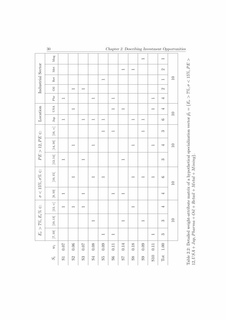
A- Create a detailed weight-attribute matrix by expanding the specializa-
tion conditions (filtering criteria), as seen in Table 2.2:
1. Stock names and weights are aligned vertically in a column
2. Filtering criteria are aligned horizontally in a row.

2.2. Weight-attribute Matrix and Impact Matrix 29
3. Transform the numerical criteria into several numerical intervals. For
example, the criteria ER > 7% is to be translated into several intervals
like shown in Table 2.3.
4. For non-numerical criteria include a column for each category: USA
and Japan for the geographical criteria have two separate columns, and
each sector of the industry has its independent column.
5. Insert a 1 in the squares where the attribute is valid for each stock.
30 Chapter 2. Describing Investment Opportunities
Er>
7%,E
r%
∈:σ<
15%,σ
%∈:
PE
>12
,PE
∈:Location
IndustrialSector
Si
wi
]7,1
0[
[10,1
3[
[13,+
[]0,1
0]
]10,1
5[
]12,1
4[
[14,1
6[
[16,+
[Jap
USA
Phr
Oil
Ret
Met
Mng
S1
0.07
11
11
1
S2
0.06
11
11
1
S3
0.07
11
11
1
S4
0.08
11
11
1
S5
0.09
11
11
1
S6
0.11
11
11
1
S7
0.14
11
11
1
S8
0.18
11
11
1
S9
0.09
11
11
1
S10
0.11
11
11
1
Tot
1.00
33
44
63
43
64
42
12
1
10
1010
1010
Tab
le2.2:Detailed
weight-attribute
matrix
ofahypotheticalspecializationvector�p1=
{Er>
7%,σ
<15
%,P
E>
12,U
SA+
Jap,P
harm
a+
Oil+
Retail+
Metal+
Mining}.
2.2. Weight-attribute Matrix and Impact Matrix 31E
r>
7%,E
r%
∈:σ<
15%,σ
%∈:
PE
>12,P
E∈:
Location
IndustrialSector
Si
wi
]7,1
0[
[10,1
3[
[13,+
[]0,1
0]
]10,1
5[
]12,1
4[
[14,1
6[
[16,+
[Jap
USA
Phr
Oil
Ret
Met
Mng
S1
0.07
00
.07
.07
0.07
00
.07
0.07
00
00
S2
0.06
00
.06
0.06
0.06
00
.06
0.06
00
0
S3
0.07
00
.07
.07
0.07
00
.07
00
.07
00
0
S4
0.08
0.08
00
.08
0.08
0.08
0.08
00
00
S5
0.09
.09
00
0.09
00
.09
.09
00
0.09
00
S6
0.11
.11
00
.11
00
0.11
0.11
.11
00
00
S7
0.14
0.14
0.14
0.14
00
0.14
00
.14
0
S8
0.18
00
.18
0.18
0.18
0.18
00
00
.18
0
S9
0.09
0.09
00
.09
00
.09
.09
00
00
0.09
S10
.11
.11
00
0.11
0.11
00
.11
.11
00
00
tot
1.00
.31
.31
.38
.39
.61
.28
.43
.29
.58
.42
.37
.13
.09
.32
.09
1.00
1.00
1.00
1.00
1.00
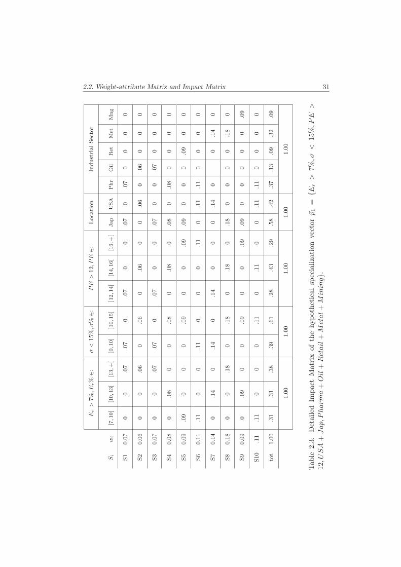
Tab
le2.3:Detailed
Impact
Matrix
ofthehypotheticalspecialization
vector�p1=
{Er>
7%,σ
<15
%,P
E>
12,U
SA+
Jap,P
harm
a+
Oil+
Retail+
Metal+
Mining}.

32 Chapter 2. Describing Investment Opportunities
B- Create a detailed Impact matrix by multiplying the weight matrix [wi]
by each category (column) of the Criteria matrix, as seen in Table 2.1 and
in Table 2.3. The resulting is an Impact matrix showing the weights of each
stock Si per each category. Please note that the sum of weights per category
should be equal to 1, which is the budget constraint.

2.2. Weight-attribute Matrix and Impact Matrix 33
As an illustration, the Expected return impact matrix [IMPexp.ret] was ob-
tained by multiplying the transpose of the weight matrix [wi] by the Expected
return weight criteria matrix [Cexp.Ret]:
[IMPexp.ret] = [wi]−1 x [Cexp.Ret] and where:
[wi]
−1 =[.07 .06 .07 .08 .09 .11 .14 .18 .09 .11
]
[Cexp.Ret] =
⎡⎢⎢⎢⎢⎢⎢⎢⎢⎢⎢⎢⎢⎢⎢⎢⎢⎢⎢⎢⎢⎣
0 0 1
0 0 1
0 0 1
0 1 0
1 0 0
1 0 0
0 1 0
0 0 1
0 1 0
1 0 0
⎤⎥⎥⎥⎥⎥⎥⎥⎥⎥⎥⎥⎥⎥⎥⎥⎥⎥⎥⎥⎥⎦
and: [IMPexp.ret] =
⎡⎢⎢⎢⎢⎢⎢⎢⎢⎢⎢⎢⎢⎢⎢⎢⎢⎢⎢⎢⎢⎣
0 0 .07
0 0 .06
0 0 .07
0 .08 0
.09 0 0
.11 0 0
0 .14 0
0 0 .18
0 .09 0
.11 0 0
⎤⎥⎥⎥⎥⎥⎥⎥⎥⎥⎥⎥⎥⎥⎥⎥⎥⎥⎥⎥⎥⎦
Which is shown in Table 2.3 in the first left quadrant. The same methodology
applies to all the criteria included in the specialization vector until the final
impact matrix is reached.
It is worth noting that the attributes included in the specialization vector
�p1 of this example are arbitrary as well as the weights used which are for
illustration purposes.
In theory, the manager or the investor would specify his requirement for
a portfolio with a maximum of n stocks with m attributes. Those attributes
can be numerous.
In theory m can be greater then n, in the sense that the manager might
decide to include 10 stocks in his portfolio with 15 different attributes or
criteria. Each stock chosen in the portfolio must have each and every criteria
attribute or else it would have been filtered out.

34 Chapter 2. Describing Investment Opportunities
On the other hand, using the individual impact matrix per stock, we have a
glimpse description of the contribution of this stock to the portfolio. Consider
for example stock s3 as an illustration. Its impact matrix is the following:
IMPs3 = [0 .08 0 .08 0 0 .08 0 .08 0 .08 0 0 0 0]
Assuming linearity of weight aggregation, we can sum up all impact matri-
ces of the individual stocks,[IMPsi ] to reach the portfolio impact matrix,
[IMPportf ]:
[IMPportf ] =n∑
i=1
[IMPsi ] =
[IMPportf ] = [.31 .31 .38 .61 .39 .28 .43 .29 .58 .42 .37 .13 .09 .32 .09]
So when we see this matrix we can have an idea or a description of what
the portfolio is and we can compare two different portfolios assuming the
specialization vectors have the same filtering criteria.This impact matrix re-
flects the impact of the aggregate weights of the portfolio on each and every
attribute.
2.3 Introduction to Portfolio Description Using Con-
centration
At the level of portfolio information, many helpful insights can be drawn from
an impact matrix. Not only it shows, at a glance, the proper geographical
distribution within the portfolio but also the investor can see where is his
wealth allocated and how it is distributed. Looking at the tables 2.2 and
2.3 we can have an idea of the contents of the portfolio. At a glance we can
describe it and draw some first hand conclusions.
• The portfolio has slightly more weight on the high return bracket of
Er > 13% because it has 4 included in this group compared to 3 stocks
in each of the other remaining two Expected return groups.

2.3. Introduction to Portfolio Description Using Concentration 35
• Half of the portfolio stocks have a standard deviation between 15% >
σ > 10%. However, this is reflected in 0.61 of cumulative weights of
those 5 stocks.
• 6 stocks are Japanese and 4 stocks are from USA. This is reflected also
in the weights where 0.58 in weight represent Japanese stocks.
• 4 out of the 10 available stocks belong to the pharmaceutical industry
sector with 0.37 in weight against 0.13 to its nearest sector, oil and gas.
• On the weight side, we observe that S8 is the heaviest with 18% weight
contribution in the portfolio followed by S7 with 14%. The lightest stock
is S2 with 6% in weight contribution.
• S8 + S7 + S6 = 43% representing slightly less then half of the wealth
invested in the portfolio.
A lot of conclusions can be drawn from the simple observation of Tables
2.2 and 2.3 above. It is a multidimensional impact matrix showing where
the influences of the weights are and where the most of the stocks are, or in
other words, this matrix gives an idea on the concentration of some attributes
around some stocks.
From the matrices depicted we can see the specialization of the portfolio
and its concentration.
We can observe that the portfolio above is concentrated around 3 stocks
S8, S7 and S6 and that it is specialized in Japanese stocks rather then US
stocks to a certain degree. It is also a pharmaceutics and metallurgy special-
ized portfolio with most of its stocks exhibiting a standard deviation between
10% and 15%.
This qualitative description based on the observations of the tables of the
weight-attribute and impact matrices give a rapid idea on how the portfolio
is constituted and can be a handy tool to compare two different portfolios,
at least from the stocks and their attributes. We can tell exactly that one
portfolio is more concentrated then another in a certain given attribute. We
can also say with confidence that the portfolio is concentrated in weights

36 Chapter 2. Describing Investment Opportunities
around some identified stock. What we need is to quantify this “degree of
specialization” and this “degree of specialization”. We will derive concentra-
tion and specialization measures that quantify our description, allowing the
investor to compare with a fair degree of confidence across several portfolios
and investment platform.
2.4 Concluding Remarks
The investor interest is in the future performance of his investment, and the
future performance depends on the horizon of the investment and the time to
the horizon from the day of inception of the portfolio. For that reason, a lot
of attention has been given in the literature to the estimation of the future
returns. A lot of attention is also given in the literature putting the quality
of these estimates into doubt, in fact, when the estimates are not reliable,
using optimization processes will result in unreliable output that will tend to
concentrate the portfolio in very few assets.
Their is an obvious need to construct an additional descriptor, aside the
usual tool-kit of investment professionals, i.e. the return and variance, to
include an estimation error-free measurement to describe an investment port-
folio. A usual strategy followed by investors to lower the estimation error, at
least intuitively, is to allocate 1/n of the wealth in each chosen asset. In fact,
(DeMiguel et al., 2009) in their paper on the 1/n allocation strategy show
that, a 1/n allocation strategy will reduce the impact of estimation error.
However, even if an investor decides to allocate 1/n of his wealth in each
stock, choosing to minimize concentration level, the portfolio remains biased
in his initial choice of the attributes of the assets to be included in his portfo-
lio. The screening or specialization vector introduced in this Chapter, shows
clearly that if an investor wants to allocate with optimal diversification strat-
egy, which is intuitively a 1/n allocation, the choice of the assets to be included
in his portfolio should engulf all the possible existing assets in the investment
Universe.
The impact matrix generated by the choices of the investor describes the

2.4. Concluding Remarks 37
portfolio with measures, concentration and specialization, that are estimation
error free since the characteristics of the attributes measured are not time
dependent but rather intrinsic to the assets and very rarely change4.
4we assume that those attributes do not change with time, unless a merger and acquisitionhappens and the company changes its industry sector or geographic location among all otherpossible attributes.


Chapter 3
Concentration and
Specialization Measures
Someone told me that each equation I included in the book would halve
the sales.Stephen Hawking
The aim of this chapter is to introduce the concentration and specialization
measures used in the study of welfare and income inequality. This chapter
answers Research Question 2. It will explore the related literature review
on those measures. Additionally, this chapter will define the principles and
characteristics that a concentration and a specialization measure,applied to
an investment portfolio, should have that will result in relevant and useful
information for the investor. The chapter will conclude by specifying those
measures of concentration and specialization that we believe they are adequate
to be applied to an investment portfolio, from the standpoint of an investor.
39

40 Chapter 3. Concentration and Specialization
3.1 Concentration and Specialization Measures in
the Literature
As we saw earlier in Chapter 2, the concepts of concentration and specializa-
tion are complementary. In fact, specialization is a concentration in attributes
or properties. It is the result of a filtering process where an investment uni-
verse is subjected to a set of desired attributes resulting in a specialized
sub-universe1. The concept of concentration is widely applied in economics
and income theories. It is often used as a tool to define and detect a group of
dominant industries in a market or to study the income distribution between
nations or within societies as well as defining the poverty lines and inequality
of a related social situation. Inequality as a measure is widely used in welfare
studies and is a term indicating uneven distribution of wealth between citi-
zens. It is considered that when inequality exists among members of a society,
some form of wealth concentration must have lead to it. Hence, in some texts
Inequality and Concentration are used interchangeably. In fact, when equal-
ity of income exists among members of a society, no wealth concentration is
observed. In our thesis we will use the term concentration. However, in this
section, the term “inequality” will be used when it is referred to by the author
of the literature under review. The concepts of inequality and concentration
are further discussed in Section 3.2.
Various theories concerning international trade, economic geography and
socio-economic policies use the concept of concentration as a quantitative
tool. As mentioned earlier, industrial specialization of regions uses inequality
or concentration measures to describe the industrial specialization of a region
compared to other regions in a geographic area. In the coming subsections we
will explore the concentration and the specialization measures in the literature
and we will pave the way to derive from the available economic research, the
general properties that a concentration and specialization measures, applied
1Our discussion hinges on concentration and specialization in investment portfolios. Theconcept of specialization, or geographical and spatial specialization, widely used in industrialspecialization of regions, relates to the attribute of industrial specialization of a given region,comparing its industrial output of some specific industrial sector with other regions’.

3.1. Concentration and Specialization Measures in the Literature 41
to investment portfolio, must have.
3.1.1 Measures of Concentration.
Early works on inequality are based on the work of Max Otto Lorenz (Lorenz,
1905) and what is known as the Lorenz curve. Essentially, the Lorenz curve
represents the relationship between the cumulative portion of the population
and the cumulative amount of a given resource or a scalar of interest held by
the population. The scalars, like individual income, units of production or
market share per company etc. are ranked in increasing order and the cu-
mulative participation of each rank is then calculated. For example, consider
a population of n individuals and consider a scalar x that is a positive and
natural number2 associated with a measurable attribute like income level,
units of production or market share. For each individual i, i = 1, . . . , n we
associate a value xi where the vector x1, . . . , xn is sorted in ascending order of
magnitude. The Lorenz curve is then obtained by plotting the points ( kn ,SkSn
),
with k = 0, . . . , n and with S0 = 0 and Sk =∑k
i=1 xi representing the at-
tribute cumulative sum of the first k individuals of the population. Joining
the points yields the curve M connecting the origin at (0, 0) with the point
(1, 1), as shown in Fig 3.1
2In our thesis, we will be dealing essentially with positive and natural numbers associatedwith a measurable attribute (in our case the weights of the individual stocks in a portfolio).The concentration measures encountered in the literature mainly deal with positive numbers.When negative numbers are involved (like negative income for example), it is obvious thatthe coefficient or index of concentration takes value greater then one, as demonstratedtheoretically by Hagerbaumer (1977) and empirically by Pyatt et al. (1980). Many researchdealt with reformulating and normalizing some concentration measures to include negativeelements, we mention mainly the reformulation of the Gini index to include negative incomeby Chen et al. (1982).

42 Chapter 3. Concentration and Specialization
Figure 3.1: The Lorenz curve M , showing the line of perfect equality.
The Lorenz curve M is always below the line of total equality since Sk =∑ki=1 xi becomes Sk =
∑ki=1
1n = k
n only when total equality is achieved.
Greater inequality among members of the population is registered by the
deviation of the Lorenz curve from the total equality line. Maximum concen-
tration or total inequality occurs when all of the attribute (wealth, income,
production, etc.) is concentrated in one single member of the population and
the plot ( kn ,SkSn
) is reduced to a single point (1, 1) representing the maximum
concentration or the maximum inequality3.
During the same period of time, around 1905 a relevant scientific event also
took place in the University of Bologna, Italy. Corrado Gini defended his doc-
toral thesis on the statistical analysis of birth by gender. The Lorenz (1905)
paper mentioned earlier greatly influenced further development in stochas-
tic dominance, probability and distribution theories, while Gini focused on
income inequality that was primed by his criticism of the Pareto inequality
3Note that it is intuitive to find graphically the point on M representing the averagevalue of the attribute measured. Since the average of the scalar is 1/n and since the totalequality line is a straight line with slope 1/n, we conclude that the tangent to the curve M,parallel to the total equality line, is tangent at a point representing the cumulative count ofthe population whose cumulative value of the attribute is the average of the distribution.

3.1. Concentration and Specialization Measures in the Literature 43
parameter. This led Gini later on to formulate his proposition of the famous
inequality ratio, or what we call today the Gini index or, simply, the Gini of
a distribution and which he published in 1914 (Gini, 1914).
Those two analytical elements, namely the Lorentz curve and the Gini
index are widely used in welfare, income and generally in most economic
studies concerned with distribution, dominance or deviation from a standard:
poverty line (Dalton, 1920), poverty and deprivation (Sen, 1976), Internet
bandwidth usage (Ogryczak, 2007), industrial specialization versus geographic
concentration (Ceapraz, 2008) and (Aiginger and Davies, 2004), the effect of
merger and acquisitions between firms and oligopoly (Watt and de Quinto,
2003) or political science (Taagapera, 1979) to cite some examples.
Various developments and reinterpretation of the Lorenz-Gini initial ap-
proaches resulted in new indexes and measurements of inequality or concentra-
tion using a welfare economic approach pioneered by Dalton (Dalton, 1920),
Kolm (Kolm, 1969) and Atkinson (Atkinson, 1970).
In this line of development, Camilo Dagum has published three seminal
papers on personal income distribution, inequality measures between income
distributions and the relationship between income inequality measures and
social welfare functions. In fact his model of income distribution (Dagum,
1977) is a continuous probability function defined over all positive numbers.
This marks the start of creating special distribution functions to cater for
and explain inequality as such. Dagum (1980) (and later 1990) suggested a
measure of the direct economic distance between income distributions to as-
sess relative affluence between the subgroups of the population under study.
In this paper, Dagum uses the Gini index as a measure of inequality (Gini,
1914). The Dagum distance measure evaluates the economic distance, in
units of monetary measurement, between the subgroups under study. This
distance is directional and is calculated from observed data and hence, it is
not an estimation. It describes the wealth distribution (and consequently the
wealth distribution function) among the members of the society under study,
divided into independent non-overlapping groups. For example, the wealth
distribution distance can be captured between males and females, or between
44 Chapter 3. Concentration and Specialization
the northern–southern–eastern and western areas of a country. Traditionally,
theses measures were assessed using statistical measurements like the median
or average of the distribution considered. The simplicity in using the Gini
ratio or index in such a measurement is that the calculation does not make
any assumption on the distribution itself and hence it is not an estimated
value but rather a precise, estimation error free measurement. In a further
development, Dagum suggests a decomposition of the Gini index (Dagum,
1997b) among three different ratios, namely: the Gini inequality ratio within
a subgroup of the population, the contribution of this subgroup to the to-
tal inequality ratio of the whole population and the distance between the
inequality between subgroups of the population. A similar approach to de-
composing inequality measures was presented by Bourguignon (Bourguignon,
1979) (and later 1988) whose ratio is based on the log of the proportion of
inequality within a subgroup to the average inequality within the full group.
In his book “Measuring Inequality”, Cowell (2009) describes various meth-
ods of measuring income inequality in a population. He derives a general
entropy measurement which is also found in various literatures of information
theory. Cowell derives a measure of the “degree of disorder” within a sys-
tem according to the probability distribution of the events in question within
the system, a measurement defined as entropy. Theil (1967) argues that the
entropy concept is a useful measurement of inequality if the concept of n
possible events is re-interpreted as n members of the population.
Although the available literature on income distribution is extensive, very
limited research was found related to portfolio concentration levels or mea-
surement. For instance, building on the entropy concept, Kapur and Ke-
savan (1992) proposed an entropy maximization model and a cross-entropy
minimization model as a variation of Markowitz model. Later, Raghunathan
(1995), uses entropy to describe the diversification4 of companies and to qual-
4Diversification is essential in portfolio management and in portfolio description. Theterm diversification is used in economic and welfare study to describe a non-concentratedset of elements but not necessarily an equally distributed attribute among the elements ofthe set. By intuition it is assumed that a diversified set is a set whose total value is dividedequally among all members of the set (the 1/n allocation scheme, see (DeMiguel et al.,2009)). We will further explore diversification measures in a portfolio in coming sections of
3.1. Concentration and Specialization Measures in the Literature 45
ify the amount of concentration of a particular firm in a market or in an
industrial sector. He also used the entropy measure to compare a firm’s di-
versification (the different output it produces against focusing on one unit of
produced output) against its level of specialization and concentration. Meucci
(2009) describes a diversification distribution and later derives a diversifica-
tion index of the portfolio based on the entropy of the distribution.
As for concentration levels in investment portfolios, the literature available
predominantly relates to measures of diversification in portfolios. Heterogene-
ity of markets was explored by Pouchkarev (Pouchkarev et al., 2006), applying
the methodology of Portfolio Opportunity Sets5. A related paper on concen-
tration of portfolio based on the bias of local versus foreign investors (due
to asymmetry of information available to locals versus the non-locals, biasing
the portfolio selection and concentrating it in few local stocks) was discussed
by Ivkovic et al. (2008) using the HHI index as a concentration measure.
Portfolio selection based on fuzzy cross-entropy was explored by Qin et al.
(2009).
Still, some articles relevant to our study of concentration in investment
portfolios must be mentioned, namely, an unpublished paper by Matarazzo B.
et al.6, on pretension level in a portfolio and a published paper by Simonelli
(2005) on the indeterminacy in portfolio selection. Important portfolio ap-
proaches were made by Mussard and Terraza (2004) by arguing that the
concentration of returns of a particular security around a certain value is a
this thesis.5POS: Portfolio Opportunity Sets, is the set of all possible portfolios made of a given
number of individual stocks.6Benedetto Matarazzo, Salvatore Greco and Jaap Spronk. This is an unpublished study
that we were able to explore thanks to the generosity of its authors. The concept of Pre-tension is introduced by the authors and is defined as the degree of concentration of weightof a stock within a portfolio. The more weight an investor puts on a particular stock, themore “pretension” he has that this stock will outperform the others. If an investor has nopretension on any particular stock, the he will use a 1/n weight distribution, a situationof total equality of weights or of minimum concentration, and hence the authors definedthis as a “zero pretension level”. The concept of pretension level reflects the proportion ofwealth an investor “bets” on one stock over the others and reflects the pretension he hasthat those stocks, subject to his preference and hence where he put his bet, are going tooutperform. The pretension level they defined is measured with the HHI index.

46 Chapter 3. Concentration and Specialization
measure of the risk of this security, since it defines the dispersion7 of the
values of returns around a central value (the average) and hence their stan-
dard deviation. Mussard et al. used the Gini index and its decomposition
(suggested in the central work of Camilo Dagum) into concentration within
a subgroup of the set, the concentration of the whole set and the distance
between the concentrations between each subgroup.
An interesting development in portfolio concentration measures was pre-
sented by Brands et al. (2004) suggesting the usage of a divergence index8 to
measure the amount of divergence between the concentration of the portfolio
compared to the market concentration, which is used as a benchmark. From
his side, Ogryczak (2007) dealt with allocating resources among competitive
activities using inequality measures approach. This suggests using the same
logic to allocate the wealth in different securities to form a portfolio.
The concentration measures used and researched in the past literature
focus primarily on equality which suggests a natural wealth allocation of 1/n
within a portfolio. But logically this is not the case in real life investment
situation. In fact investors have subjective as well as objective preferences of
investing in some stocks more than in some others or to invest in a certain
sector or sectors that they believe would maximize their return for the risk
they accept to take, which automatically suggests a bias to the 1/n allocation
strategy.
7The statistical dispersion of returns is defined as the asset-weighted standard deviationof individual stocks’ returns within a portfolio.
8The Divergence index is the sum of the squared difference between the individual weightsof a portfolio and a benchmark portfolio, taken as a reference (usually the Market portfolio).D =
∑(wportfolio
i − wbenchmarki )2

3.1. Concentration and Specialization Measures in the Literature 47
3.1.2 Measures of Specialization.
The development of the field of geographic economics9 has produced a clear
interest in creating indicators to reflect the geographic industrial output or
production concentration or what the geographic economist call: The re-
gional agglomeration of industrial production, i.e. the regional concentration
of the production and the industries specialization that produces this indus-
trial concentrated output. The work of (Krugman, 1991a) and (Krugman,
1991b), while studying the relationship between transportation costs and re-
gional industry specialization, presented a new index of specialization: The
Krugman Specialization Index10.
A parallel approach to defining concentration and specialization in na-
tional industrial sectors was elaborated by Ceaparz, (Ceapraz, 2008). In his
study of the productive Romanian industrial sectors, he discusses the com-
petitiveness of the Romanian industries within the European Union, by using
both the Hirschman-Herfindahl index (HHI) of concentration and the Gini
index at the same time. The use of both indexes11 allows Ceapraz to as-
sess and describe the economic integration at a national level as well as to
explain and describe the regional and geographical industry concentration
in the country. However, the research on industrial specialization shows a
certain differentiation between absolute and relative specialization.
9In our research we have detected a philosophical dispute between the concept of “Geo-graphic Economics” and “Economics Geography”, which does not seem to be settled prop-erly. Far from taking sides in such a philosophical and epistemological dispute, we meanby Geographic Economics the economics of regional or geographic industrial output orproduction. In this respect, our literature review shows that the subject of Economic Ge-ography has triggered an interest in measuring industrial agglomeration and specializationlike (Krugman, 1991b), (Ellison and Glaeser, 1997), (Midlefart-Knarvik et al., 2000) and(Hallet, 2000). The majority of these indexes or measures are based on, or are variations ofthe Gini index.
10The Krugman Specialization Index is a widely used for measuring specialization. Basi-cally, it is the standard error of industry shares, i.e. it calculates the share of employmentwhich would have to be relocated to achieve an industry structure equivalent to the averagestructure of the reference group.
11In this thesis we will use indexes and/or indices as the plural of the world index: Bothindexes and indices are acceptable plurals for “index” in English–and in that order of pref-erence today (Authority: Oxford English Dictionary and Merriam-Webster Dictionary.)

48 Chapter 3. Concentration and Specialization
Absolute and relative specialization measures The related literature
focuses mainly on two different group of indexes to assess and measure the
specialization or regional industrial localization as reflected in the works of
(Bickenbach et al., 2013), (Palan, 2010) and also (Bickenbach and Bode, 2008).
(Aiginger and Davies, 2004) describe the absolute specialization measure as
reflecting the volume of output share of the country relative to the number
of industries in that country. This will permit saying, for the sake of illustra-
tion, that Italy is specialized in textiles and Spain is specialized in olive oil
production. This measure is considered absolute because it does not compare
the sample at hand with any reference group (like comparing Spain to the
EU output for example). The relative measure of specialization compares
the reference data (industrial output, employment, production . . . etc.) of
a geographic area (the EU for example) with the regional data under study.
Hence we can fairly conclude that the absolute measure of specialization com-
pares the reference region to a hypothetical 1/n distribution or to an equally
weighted hypothetical reference data whereas the relative measurement of
specialization compares the region under study with a certain reference en-
tity that is or is not related to the sample under consideration.
Empirical and theoretical studies state that the Gini index is widely used
to measure the absolute specialization of a region as well as the relative spe-
cialization with contradictory results as explained by (Bickenbach et al., 2013,
p. 1) and (Palan, 2010, p. 22)12.
3.2 General Properties of Concentration Measures
As discussed earlier, inequality is an expression of a situation where concen-
tration is present: the closer a set distribution is to total equality the smaller
the concentration level of this distribution. Concentration is a measure of
inequality. This idea stems from the fact that if most of the values of an
attribute, within the set under study, are concentrated around one value,
12If entries with infinitesimal weights are added to the sample, the specialization of thesample is altered drastically because the reference 1
nhas changed.

3.2. General Properties of Concentration Measures 49
then less equality exists between the elements of the set. It follows that if a
set’s attribute value is the same for all of its elements, hence total equality
distribution, the concentration is minimum.
As Coulter (1989) defined it in his book, concentration is a measure of
inequality. In essence, it is the degree of difference between the shares of the
elements or components of the system. This is the same as saying that an
inequality measure determines the amount of units to be transferred among
elements of a system to reach perfect equality. However, concentration is
concerned with locating this surplus among elements of a system13.
Variance is a measure of distance between the elements of a set and the
average value, expressed in terms of the square of the difference. Yet, in our
study, variance is not a useful measure of concentration. In fact were we
to double the value of the attribute under study, for example to double the
value of money allocated in each stock of the portfolio, the variance would
quadruple and the mean would double14. However the shape of the Lorenz
curve related to this portfolio will remain unchanged. Therefore it is essential,
in introducing the concept of concentration in an investment portfolio, to
determine the following factors:
• What concentration measure or measures will be used and why? What
are the desirable characteristics for a measure of concentration?
• How will these measures describe the portfolio? Applying the concentra-
tion index or indexes chosen must add value in describing the portfolio
at hand. What dimension of the portfolio will be measured (i.e. what
concentration are we measuring)?
13In fact, Coulter (1989) specifies that a typical inequality index gives the same weightto numerous tiny differences as it does to one or two large differences among elements of asystem, all other things being equal. The key difference, as he states, between inequalityand concentration is the location of the surplus (and deficit) created by inequality.
14It is to be noted that, however the standard deviation, as the square root of the variance,would remain in scale with the value of dispersion in the data, we will not use it as a measureof concentration because of its dependability on the scale of measure, as outlined in thetext.If , as expressed, the amount of income perceived by each unit of the sample doublesthe inequality among the units remains the same, but the measure of concentration (herevariance as suggested) will quadruple, while the concentration remains unchanged.

50 Chapter 3. Concentration and Specialization
3.2.1 Technical characteristics and desirable properties of con-
centration measures.
In this respect, we point out the existence of many concentration measures
applied in economic research, social welfare, industrial specialization and even
chemistry and physics. As stated by Bickenbach and Bode (2008), choosing
between measures of concentration is indeed choosing between the different
definitions of concentration that were applied to derive such measures. Any
inference or conclusion drawn from the results of a concentration or special-
ization measure we will use or decide upon in our thesis is interpreted with
regards to the definition of the concentration and specialization we decided
to establish in order to describe an investment portfolio, since the measures
we decide to choose will reflect our definitions that we determined of concen-
tration and specialization in an investment portfolio.
A variety of criteria are used to choose between the various concentration
measures available. However, we believe the measure of choice should be at
least a) relevant to the attribute or dimension to be measured, b) it should
contain enough “information” to draw conclusions, c) it must be simple and
sufficiently easy to use, d) it should have an acceptable interpretability i.e.
it should have a defined upper and lower bound (like 0 and 1 and not 0 and
∞ for example) and finally e) it should be a ratio rather then an interval
measurement. In what follows, we will shed more light on each characteristic
we mention in this paragraph.
Relevance For every system containing N elements and with a known dis-
tribution of the values of an attribute A to be measured there should
be one and only one value for the index used. Therefor, indexes with
a zero denominator are non-relevant since they have an undefined or
infinite value at that point. Indexes using mode or median as part of
its components would yield non-relevant results in bimodal or uniform
distributions.
Information The index of choice should provide the maximum possible in-
formation about the distribution it is describing. This means that the

3.2. General Properties of Concentration Measures 51
index chosen must reflect the rank and influence of proportionally small
elements as well as proportionally big elements. If the choice of the
index requires that the index reflects or points out the big or the small
elements then the index would be conveying the maximum possible in-
formation required.
Simplicity Although computations are simple today using computers, an in-
dex is preferably simple to use, easy to calculate and straight forward to
interpret. Indeed among all possible and existing concentration indexes,
the simpler ones are usually preferable, ceteris paribus.
Interpretation Interpretability is related to the upper and lower boundaries
of the index, or its maximum and minimum points. Some measures
are not bounded and can vary from −∞ to +∞ or most commonly
from 0 to +∞ (Theil, 1967). It is a common agreement among most
of the literature reviewed that the lower boundary of an index should
be zero, indicating perfect equality i.e. when each element has equal
share and hence, minimum concentration. It is also agreed that a posi-
tive increase in the measurement value should indicate a deviation from
perfect equality towards maximum concentration. Additionally, most of
the literature indicates that a measurement or an index tends towards
its maximum value of unity when one element of the system possesses
all the available shares and the remaining elements possess none of the
shares. This is very useful when comparing various sets with different
numbers of elements, bounding the values of the inequality index be-
tween zero and one. In our choice between indexes of concentration we
will use bounded indexes and will apply a normalization procedure to
make unbounded measures standardized and bounded. It is should be
noted that Cowell (2009) does not agree on the bounding of a measure
from zero to one, deeming it as a “superficial attractiveness”.
Scale of measurement the scale of measurement can be nominal, ordinal,
interval or ratio scales. Most cases would require a nominal scale to
separate the attributes (ex: north, south, east and west regions of a
52 Chapter 3. Concentration and Specialization
country) and then consider the application of a proportion measurement
to qualify the concentration of a certain attribute. As an example, we
might want to study the concentration or inequality of age distribution
in the 4 regions of a country. We would divide the country in four
nominal classes and later apply a proportion measurement to describe
the age concentration in each region. In our case, we want to classify
the stocks within a portfolio into their industrial sector (pharmaceutics,
services, oil and gas, utility, bank and financial institution etc.. . . ) and
later choose a concentration measure to compare the amount of wealth
invested in one sub-sector with respect to the others and describe where
is the investment concentrated. The investor usually requires that the
stocks admitted in his portfolio have a maximum allowable standard
deviation value of x% where this percentage reflects his risk appetite.
In this case we are interested in dividing the standard deviation values
into intervals so that we can classify each stock within its corresponding
interval. (Please refer to the tables 2.2 and 2.3 for illustration on the
interval subdivision for some attributes.). So ultimately we prefer a ratio
scale of measurement for its ease of comparison and relative formulation.
Coulter (1989), Cowell (2009) and many others researching on topics re-
lated to social welfare and distribution of income theory referred, at one time
or another, to concentration and inequality measures and derived most of the
concentration indexes utilized today. See e.g. (Pigou, 1920) and (Dalton,
1920) for the Pigou-Dalton principle of transfer, (Kolm, 1976a) and (Kolm,
1976b), (Allison, 1978) and (Schwartz and Winship, 1979) or (Rae, 1981)
as well as (Nagel, 1984). Some of the criteria derived in the social welfare
and income inequality studies are useful in describing an investment portfolio
(Examples are the Transferability Principle and the Scale Invariance Princi-
ple discussed hereafter). Some other criteria or principles like the Constant
Addition Principle, are not relevant to describing portfolios15.
15Constant Addition Principle states that concentration diminishes when a positive con-stant is added to all elements of a set. In income distribution this might present an importantuse due to the fact that some poorer members of a society might receive a constant aid from

3.2. General Properties of Concentration Measures 53
The criteria and principles found in the literature that we believe our
concentration index(es) must satisfy are:
a) The Principle of Transfers16. The Principle of Transfers states that
concentration is diminished if units are transferred from a larger share
element to a smaller share element. Cowell (2009) describes two different
states of this Principle, namely the Weak Transfer Principle and the
Strong Transfer Principle.
The Weak Transfer Principle states that for a given distribution S,
with wi = xi∑n1 xi
, being the fraction of attribute (weights in case of
a portfolio) allocated to each element si ∈ S with∑
wi = 1 as the
budget constraint, any hypothetical (positive) transfer of weight ε (in
our particular case) from a bigger weight w1 to a smaller weight w2
(w1 > w2) should reduce the measure of concentration.
More explicitly, consider w1 > w2 with w1 = w2 + δ, then any transfer
of weight from w1 to w2 , namely ε = Δw1, with Δw1 < 2δ (if not,
we will be simply swapping between the weights of w1 and w2), will
tend towards reducing inequality within the universe and hence reduces
concentration. This is the Weak Transfer Principle, it is called so be-
cause it does not quantify the amount of reduction, it just confirms the
reduction in concentration.
The Strong Transfer Principle states that in the case of a similar trans-
fer of weight from one heavier element to a lighter one, as in the weak
transfer principle, the decrease in concentration depends exclusively on
governments or other supra-national entities under some poverty eradication plan. In in-vestment portfolios however, this addition is seldom envisaged since the dynamic allocationof the wealth invested among the chosen stocks would keep the budget constraint stable ata certain initial amount invested. If the portfolio produces profit during one period, theprofit is seldom re-allocated evenly among all stocks in the portfolio but rather accordingto a different allocation criteria that would alter the share of each stock in the investmentportfolio and hence change the value of concentration.
16The Principle of Transfers is related, in our analysis to dynamic re-allocation within theportfolio, in time. The measures of specialization and concentration we propose will detectthe transfer effected in the allocation between stocks of the portfolio. For a broad commenton the Principle of Transfer please see (Hao and Naiman, 2010),(ch.4, page 44–64).

54 Chapter 3. Concentration and Specialization
the distance between the weights of both elements, i.e. it should de-
pend only on ε = δw1. In other words, the amount of reduction in the
concentration index depends only on the distance between the donor
and the receiver, regardless of their relative rank within the population
under study. It is clear that the index not depending on the ranking of
the elements in the mathematical formula will obey the Strong Transfer
Principle, whereas those indexes incorporating a ranking multiplicative
factor within their analytical expression will not obey the Strong Trans-
fer Principle, since even with the condition ε = δw1, with Δw1 < 2δ
satisfied, the amount of reduction in the index does not depend uniquely
on ε, but rather on a product involving a proportion related to the rank-
ing i of wi. In fact, the size of the change in the value of the concentra-
tion index, when a redistribution of weights occurs within a portfolio
(re-balancing of wealth distribution or reinvestment of dividends, etc
. . . ), will depend on the relative position of the individual stocks among
which the weight transfer occurred and not on the absolute value of their
weights. Hence, the transfer of weight between the 1st to the 2nd stock
in ranking does not have the same effect on the index as the transfer
of the same amount from the 20th to the 21st stock in the universe, for
example.
b) The Principle of Scale Invariance. This principle requires that if each
and every share wi of the universe under study is multiplied by the
same positive constant, the concentration measure should not change
and must remain the same. On the social economic level, not all social
scientists agree on the fact that inequality should not change if all the
elements of the society’s wealth is increased by the same positive index.
This feature is important when we consider that the multiplier could
be less then one, and is assimilated to have a similar effect as a sudden
devaluation event or an inflationary spree; it can also reflect the effect
of taxation on the income of a society. In fact many social scientists are
also concerned with the “distance” between the wealth of one individual
and the other as well as to the minimum line of poverty. In this line of

3.2. General Properties of Concentration Measures 55
thought, it is not the same to have individual A with 1000 units and B
with 5000 units of wealth and the same individual A with 10,000 units
and B with 50,000 units. The distance in the second case is much bigger
and the social scientists argue that inequality is more pronounced with
a difference of 40,000 units between A and B than when the difference
or distance was only 4,000 units, although the proportion is the same.
But in our case, since concentration is our basic concern rather then
inequality, doubling the wealth invested in each and every stock of the
portfolio will not change the description of the portfolio vis-a-vis its
concentration level, since the share of each stock with respect to the total
wealth invested remains the same. In fact, and from the standpoint of an
investor, doubling the investment in each and every stock of the portfolio
is similar to creating another portfolio of investment exactly identical
to the initial one, and hence no investment opportunity is created. We
believe, from a pure investment standpoint, that the concentration index
of the investor’s chosen portfolio and the initial index are the same, and
hence our choice of an index should focus on a scale invariant index.
It is also logical to opt for an index which is scale invariant because a
change of currency or an equivalent value of the portfolio in another
currency should yield the same concentration value.
c) The Principle of Constant Addition. This Principle states that if a
constant amount is added to each and every share of the elements of
a universe under study, the concentration must diminish (because the
inequality diminishes). The rationale behind this conclusion is easily
seen if we envisage the constant amount added to be substantial relative
to the amounts or values of each element of the universe, creating a
dilution effect on the total concentration.
In other words, when adding the amount a to each share of the system,
wi + a with a >> wi we can confidently assume that wi + a � a for all
wi. This will eventually produce a system whose elements are all ap-
proximately equal and hence reduce the concentration to its minimum:
56 Chapter 3. Concentration and Specialization
all the shares tend to have “more or less” the same value and hence the
set tends to get near total equality when the added constant grows to
a proportionally large amount. This feature of a concentration index is
sought after in social sciences and in plans dealing with poverty levels
and a minimum poverty line. The amount added to all the elements
of a universe (a fixed sum of money given to all members of a society)
will positively remove many people if not all (depending on the amount
added to the income of each defined poor citizen) from the state of
poverty determined by the minimum poverty line and hence, a social
scientist would argue that, poverty being diminished, more equality is
achieved among the citizens and hence less wealth is concentrated in the
hands of a few. This feature is not relevant in an investment portfolio
because, as mentioned earlier, any additional amount that is produced
as dividend will be dynamically allocated according to an investment
criteria rather than blindly added at equal amounts to all the elements
of the portfolio.
d) The Principle of Population: Symmetry and Sensitivity to size.
i. Symmetry of population. This principle requires that the concen-
tration measure should not depend on the number of the popula-
tion n, and it should remain constant remains constant if we merge
two populations with the same number of elements n and with the
same inequality of a certain attribute. If we measure inequality in
a particular economy with n people in it and then merge the econ-
omy with another identical one, we get a combined economy with a
population of 2n, and with the same proportion of the population
receiving any given income. If measured inequality is the same for
any such replication of the economy, then the inequality measure
satisfies the principle of population. This is not the case if we are
applying the index to an investment portfolio. In fact, merging two
investment portfolios each with n stocks and with a certain level
of weight concentration will result in a new third portfolio where
3.2. General Properties of Concentration Measures 57
concentration might not be the same if both portfolios contain at
least one identical stock or when each portfolio has a different spe-
cialization17. If both portfolios contain different stocks then the
combined portfolio will result in a 2n stocks portfolio with the
different specialization level and maybe different weight concentra-
tion measure. Additionally, assuming we have two portfolios of n
stocks each, and assuming no stock is existing in both portfolios at
the same time, combining both portfolios will not necessarily re-
sult in a portfolio with the same concentration and specialization
levels, because the stocks of each portfolio might not have exactly
the same attributes (location, industrial sector, level of expected
return, etc. . . ).
As an illustration, consider the following vector of screening at-
tributes that will produce a portfolio F1 with certain desired at-
tributes, and n stocks with an concentration index of I1:
�p1={USA stocks, non-financial Co., P/E ≥ 15, Debt/Assets ≤33.3%}.Now assume we create another investment portfolio F2 of exactly
the same number of stocks n and resulting in the same concen-
tration index value I1 = I2, changing one screening criteria from
USA market to EUROPEAN (EUR) market stocks and keeping all
other screening criteria unchanged:
�p2={EUR stocks, non-financial Co., P/E ≥ 15, Debt/Assets ≤33.3%}.It is clear that F1 and F2 do not have any common stock existing in
both portfolios at the same time. Combining both portfolios will
result in a new portfolio F3 with 2n number of stocks and with
I3 = I1⊕ I218 concentration index, but with less concentration on
17This is similar to saying that, if we add the additional dimension, from the social scienceperspective, of gender or race, then the concentration relative to these aspects will change.Just as, in the merged portfolios, the nature of the stock (its attributes), is at the heart ofthe concentration we are trying to measure.
18the symbol ⊕ is used here instead of the symbol + to avoid implying tacit additive

58 Chapter 3. Concentration and Specialization
USA stock market since the F2 contains European stock market.
Hence the Specialization of portfolio F3 is not the same as F1 and
F2. In fact F3 is the result of the following screening criteria:
�p3={USA + EUR stocks, non-financial Co., P/E ≥ 15,Debt/Assets ≤33.3%}.This screening vector yields a less specialization in USA or Euro-
pean stocks alone, but it is rather specialized in BOTH markets
and hence is different from F1 and from F2.
ii. Sensitivity to the size of population. This principle differentiates
two different types of indexes: those sensitive to the size of the
population and those which are not. Coulter (1989), defines those
indexes whose values are independent from the number of compo-
nents as relative measures of inequality, and those whose measures
are sensitive or dependent on the number of components as abso-
lute measures of inequality, as discussed by Waldman (1976). Each
category has its proper usage and caveats. This principle in par-
ticular is very important in political sciences, voting systems and
parties. The research work of Taagapera (1979), related to political
parties and voting systems, sheds an important light on the num-
ber of components of the population and the political ostracism or
concentration of power in the hands of few individuals or one party.
The concept of null components (in the case of Taagapera, the in-
dividuals who did not vote) represents a serious issue in political
sciences and might have its reflection in finance and investment as
we shall see.
• Relative indexes or those indexes not affected by the number
of the population are indexes whose extremums (minimum and
maximum) do not depend nor vary with the number of com-
ponents n. As an example, if we have a population of five
individuals where 90% of the wealth is concentrated in the
properties of the concentration index.

3.2. General Properties of Concentration Measures 59
hands of two of the five persons, then a relative index should
yield the same value if the population consists of 100 individ-
uals and 90% of the wealth is concentrated in the hands of
the same two persons. This appears to be inappropriate since,
intuitively, we know that the second population of n = 100 ap-
pears to be more unequal than the first, if we consider social
welfare as the criteria for comparison and judgment.
• Absolute indexes are those indexes depending on the num-
ber n of the population and whose extreme values depend on
n. Waldman (September, 1977) defines various types of abso-
lute indexes depending on the inclusion of null and non-null
components. It is of an importance to note the difference in
concentration, for example, in a society where a candidate in
District A won 90% of the votes with half of the potential
voters not voting (null entries) and a candidate in District B
won with 90% of the votes with no null entries registered, all
other things being equal. A relative index, not sensitive to the
number of potential voters n, would yield the same result for
districts A and B, whereas an absolute index would result in
different readings, showing more inequality in district A (Taa-
gapera, 1979).
The Principle of Sensitivity to the size of population is controver-
sial and admits subjective points of view. Consider the following
example:
In a population of 100 industries, 5 industries control 99% of the
industrial output and the remaining 1% is shared equally among
the remaining 95 industries. Many an index would reflect a pro-
nounced concentration in such a population. Now assume that the
5 controlling industries buy out the remaining minor 95 industries
and divide the 1% equally among each other, a relative index would
show perfect equality (all industries are perfectly divided among
5 players) whereas an Absolute index would tend to reflect gross

60 Chapter 3. Concentration and Specialization
inequality, because the count of null entries is taken into consider-
ation. In measuring specialization in an investment portfolio, we
want the index to reflect gross inequality, i.e. we want our index to
detect that, even if 100% of the weight is distributed equally among
5 stocks of a particular industry sector of a 100 stocks portfolio,
this portfolio is specialized in this industry sector.
This means that the index should take the null entries into consid-
eration and therefore, as per the principle of sensitivity, the index
of choice to measure specialization should be an Absolute index.
e) The Principle of Decomposability. This Principle states that, within
a population, the concentration measure should be decomposable into
the concentrations of the subgroups conforming the population. This
essentially refers to the determination of the contribution of each sub-
group to the total population under study. More precisely, the overall
concentration of a population should be expressed as a function of the
concentration within each of its subgroups and as a function of the
concentration among or between those subgroups. Particular attention
is given to this characteristic when economic and social welfare is con-
cerned. In fact, the distribution of wealth is not even between regions of
a country, or between subgroups of a population like blacks and whites,
males and females, ethnic and religious subgroups etc.. In our case, we
will consider the decomposability of our index of choice according to
the relevance of such a measure when we come to discuss it in full. It is
worth anticipating that the decomposition of a concentration measures
does not indicate the location of the concentration or, in other terms,
does not identify which subgroup is more concentrated then the other
but rather will indicate the contribution of the subgroup to the overall
concentration of the sample, like is the case in the Gini decomposition
that we will consider later in this research.
Having analyzed the various characteristics of the concentration measures at
large, the following section will further elaborate on applying the concept of

3.3. Concentration Measures for Investment Portfolios 61
measuring concentration within an investment portfolio. The ultimate goal
is to choose one or more indexes to apply them to investment portfolio that
will add a descriptive value in the tool kit available to the investor. We need
to define what we are interested in measuring and how we will be measuring
it.
3.3 Concentration Measures for Investment Port-
folios
The conceptualization of the term “concentration” is derived, as mentioned
earlier, from a wider and more generalized situation of inequality. Concentra-
tion is a dimension or a proxy of inequality, as stated by Coulter (1989). We
want to measure the degree of inequality between the elements of an invest-
ment portfolio, when the weights of the individual stocks are not all the same
i.e. when wi = 1/n. In fact, if all weights are not equal then some stocks
are attributed more weight then others. It is within this background that we
interpret concentration as a form of inequality and we want to quantify it.
However, the word concentration bares in its meaning the sense of location.
If the portfolio is concentrated then it is intuitive to say it is concentrated
somewhere. Whereas, inequality is a more generic term: we say the weights
of the portfolio are not all equal and hence there is inequality within the
portfolio, with no sense of location or cluster of weights.
The measures of concentration that we are studying are considered anony-
mous measures: They will tell us that the portfolio is concentrated but they
cannot possibly point out to the individual stocks which have more weight
then the others. When we group the stocks into attribute groups like industry
or geographical groups for example, then, as we shall see later, by decompos-
ing the particular index of concentration, we will be able to detect which
group “contributes” to the overall concentration of the portfolio. This does
not mean that the decomposition will show the “heavier” subgroup. It will
only calculate the contribution of the subgroup to the overall concentration.
If, for example, a subgroup represents 90% of the total weight (i.e. the portfo-

62 Chapter 3. Concentration and Specialization
lio is concentrated in one subgroup but the elements within the subgroup are
equally weighted, then the decomposed index shall not detect the concentra-
tion IN the subgroup, and will attribute the concentration to the remaining
10% subgroups. This is the contradictory results of the Gini decomposition
that we mentioned earlier, which renders the usage of the decomposition tech-
nique in our particular case useless). )
In this thesis we are introducing an additional measure that will describe
better an investment portfolio, along with the already existing descriptors like
expected return E(r), standard deviation of the historical returns σ(r) as well
as all other available moments of those returns. We want to look at the stocks
of the portfolio and be able to assess whether the portfolio is concentrated,
i.e. how much deviated from a neutral 1/n allocation position it is; at the
same time we want to know if the portfolio at hand is specialized in certain
attributes compared to others19.
The approach we suggest hereafter, is to describe the portfolio by looking
at the concentration that the wealth allocation exhibits and at the special-
ization of the given portfolio according to the attributes (i.e. groups within
the portfolio) specified by the analyst or the investor. However, because the
measures of concentration 20 are numerous and each one reflects a certain as-
pect of the inequality with respect to the elements of the analysis, we need to
define and specify very clearly what do we want to measure and what will this
measure add to our information on the portfolio at hand, before we venture
into choosing the appropriate measure(s) available in the research.
In practice, we are looking to assess and quantify the following additional
information related to an investment portfolio:
1. Concentration of wealth or wealth distribution profile: We need to assess
if, within the portfolio, the investor’s wealth is concentrated in a small
19As discussed earlier in this thesis those attributes are subjective to the choices andpreferences of the analyst or the investor. One given stock can have as many attributesas the analyst desires, and hence the measure of specialization relates directly to thoseattributes deliberately chosen by the analyst. In theory, a stock can have a very large setof attributes.
20Almost entirely derived from the concept of inequality of income distribution within apopulation

3.3. Concentration Measures for Investment Portfolios 63
number of stocks in detriment of the remaining stocks. This will measure
the concentration of the portfolio i.e. it will describe the distribution of
the amount of wealth allocated within it. This concentration of wealth,
when existing, can reflect the attitude of the investor towards those
stocks where the wealth is concentrated: The investor is betting more
chips on some stocks rather than on others within the portfolio (i.e.
among the stocks that he already decided to include in his portfolio)21.
We are seeking to describe the allocation strategy within the portfolio
through using a concentration measure.
2. Absolute Specialization of the portfolio: We need to assess in which
attributes is the wealth allocated. This information will describe the
amount of concentration of the wealth in a given attribute compared
to others, hence showing a dominance of this attribute over the others
with respect to its wealth allocation. This will describe the specializa-
tion of the portfolio by measuring the concentration of the attributes
or groups within the portfolio22. The concentration of the portfolio dis-
cussed above in 1. is not enough to give the analyst or the investor a
clear picture of the description of the portfolio. In fact, some stocks
move in and out of the Investment portfolio with time (e.g. transferring
the wealth of a stock from Japan that is excluded from the portfolio
to a replacing stock from the USA, will not alter the concentration but
will alter the geographic specialization). Similarly, the dynamic allo-
cation by shifting some of the wealth from a stock Si to stock Sj will
alter not only the concentration but also the specialization of the port-
folio. This transfer of wealth from Si to Sj could have increased the
specialization in one attribute of Sj while decreasing the specialization
in the attribute of Si23. The measure we choose should be able to give
21The attitude of the investor towards placing more wealth on some stocks rather than onothers, and hence creating a deviation from the 1/n neutral allocation strategy was definedas the “Pretension Level” of the investor in Appendix B of this thesis.
22Attributes like industry sectors or geographic location or family owned business, forexample. Please refer to Section 2.1.2, page 23.
23Consider that at time t0 we have a given portfolio with a given wealth allocation matrix.

64 Chapter 3. Concentration and Specialization
information on the contribution of the concentration of each attribute
to the total specialization of the portfolio.
3. Relative specialization of the portfolio: We need to compare the special-
ization of the portfolio under study with the initial Investment Universe.
Assume the investor chooses 20 stocks from the top 500 stocks of the
USA market. The specialization of his portfolio is not necessarily the
same as the initial Investment Universe from where he picked his stocks.
This comparison will allow the analyst to relate the behavior or the per-
formance of his portfolio to some specialization differences or similarities
to the initial Investment Universe 24. For example, in reference to the
USA stock market, with approximately 67 industrial sectors25 listed,
and if the portfolio contains only 10 sectors chosen out of this Invest-
ment Universe, then this choice exhibits a certain specialization that
the index Is must reflect, when comparing the the specialization of the
Investment Universe against the portfolio at hand.
Assume that, at time t1 we transfer a small amount of the wealth allocated to stock S1 (thisamount ε described in Subsection 3.2.1, a) The Principle of Transfer), which is a metallurgiccompany to stock S2 which is a retail company. We can confidently say that the portfoliobecame more specialized in retail and less specialized in metallurgic industrial sectors attime t1 after the reallocation was executed.
24We cannot conclude or infer that there is a causal relationship or a relevant correlationbetween the performance of the portfolio and its specialization and/or concentration mea-sures. Our study does not deal with this interesting issue that we believe is the subject ofmore thorough research in the future. This particular direction of studying the correlationbetween performance and concentration and specialization falls outside the scope of ourthesis.
25Using classified sub-sectors according to a commonly used classification system likethe GICS or the NAICS (GICS stands for Global Industrial Classification Standard andis an eight digit classification number that is used in the CRSP/COMPUSTAT marketdata base). A common practice is choosing the industrial sectors using GICS (sometimesappearing as GIND and SUBGIND in the database mentioned) to a six-digit filtering,resulting in approximately 67 different industrial sectors listed in the CRSP/COMPUSTATdatabase. NAICS stands for North American Industrial Classification Standard, and is asimilar classification system used mainly by banks and governments to classify the industrialactivities of companies.

3.4. Choosing the proper indexes to measure Concentration and Specialization 65
3.4 Choosing the proper indexes to measure Con-
centration and Specialization
We have at hand an investment portfolio consisting of stocks with a weight al-
located to each stock and a investor-defined attributes that will subdivide the
portfolio into attributes grouping. Based on a hypothetical portfolio shown in
Table 2.1, we created consequently the weight-attribute matrix in Table 2.2
and the subsequent impact matrix in Table 2.3, pages 30 and 31 consecutively.
The data we have at hand is: the individual stocks, their weights and their
attributes. When we group the stocks with respect to their attributes as in
the weight-attribute table mentioned, we can have additional data: number
(count) of stocks per group, individual stock’s and total weight per group.
This available data will be used to determine the concentration and the spe-
cialization of the portfolio. The indexes or measures we choose to produce
the results must obey to a set of criteria that we define hereafter, so that
the index chosen reflects the best the scalar we want to measure and use in
representation of measuring the concentration and the specialization of the
portfolio.
3.4.1 Determinants of choice for a concentration measure ap-
plied to investment portfolios.
Earlier in this chapter, we gave a general overview of the selection criteria and
the desired principles for concentration measures. In this subsection, we will
narrow down the choice of measures available by deciding upon which princi-
ples and criteria are most related and applicable to an investment portfolio.
• We require to measure the concentration of the weights of n stocks
composing an investment portfolio without any consideration to the
attributes grouping involved. Hence the decomposability of the index
Ic26 is not a relevant feature for the chosen concentration measure.
26We will denote the concentration index by a generic representation Ic in this section,before a proper concentration index is chosen.

66 Chapter 3. Concentration and Specialization
• We require to assess to which degree is the distribution of the wealth
allocation deviant from an equally weighted portfolio with all its weights
wi, i = 1, . . . . , n = 1/n. The biggest a particular weight is, more devi-
ation from the 1/n allocation exists, and hence, more concentration is
exhibited by this distribution. We need an index that emphasizes the
effect of “big” weights. It appears that an index with an exponent on
the weights in its formula composition will amplifies the effect of this
deviation from 1/n.
• Another relevant criteria is that we require the concentration measure
Ic to obey the weak transfer principle discussed in Section 3.2.1, i.e.
the concentration measure of our choice should diminish if a transfer
of weight occurs from a higher share to a lower one. This feature is
desirable because it will reflect, in a time panel data, the changes in
dynamic allocation within the existing stocks in one single measure27.
Additionally, the concentration should diminish more if the distance
between the “donor” and the “receiver” is bigger. This is the strong
transfer principle. This means that, the more the difference between the
higher share and the lower share, the more the impact on concentration.
This will reflect the nature of the reallocation, once it happens and
will add to the relevance of the measure we are choosing: Not only the
concentration diminishes when a transfer occurs from a higher to a lower
share, but also it diminishes even more when the distance between the
higher and the lower share is bigger. This in fact proxies the rank of
the stock within the portfolio: The concentration must diminish more
if the difference in rank between the larger and smaller stocks is bigger.
In a portfolio of n stocks, ranked in a descendant sorting, from the
highest S1 to lowest weight Sn, a transfer of ε from S1 to Sn diminishes
the concentration more then the same transfer of ε from S1 to Sm with
m > n.
27The measure of concentration will not detect the reallocation of wealth from a stockthat is excluded from the portfolio to a new stock. If the weight reallocation is the same, i.e.if the weight distribution is the same, the concentration measure will remain unchanged,although one stock was replaced with another.

3.4. Choosing the proper indexes to measure Concentration and Specialization 67
• The measure of choice should be scale invariant. In fact, if the investor
decides to double his stakes in all the stocks, the measure of concentra-
tion should yield the same result. However, if the investor decides to
add to his stakes a constant amount to all the stocks, then intuitively
the measure of choice should reflect a diminishing in the concentration.
At the limit, if the constant amount Wi added to each and every stock
is very big compared to the wealth wi already allocated to each, i.e.
Wi >> wi, this addition tends to smooth out the differences between
the stocks because the distribution of weights will tend to an equally
weighted distribution with Wi + wi ≈ Wi when Wi >> Wi.
• The measure of concentration Ic we require should not necessarily be
sensitive to the size of the population involved nor to the symmetry of
the population. The set of data we have at hand is a finite set, consisting
of the weights of the stocks included in a portfolio of investment: wi with
i = 1, 2, . . . , n and where n, the population size, is the number of stocks
in the portfolio. We also know by definition, that the concentration
level is minimum when the stocks are all equally weighted, i.e. if the
budget constraint is 1 as per definition, then this condition is met when
each individual weight is equal to wi = 1/n for all i.
The determinants of choice for a proper concentration index to be ap-
plied to an investment index are not necessarily exhaustive nor exclusive. As
stated earlier, besides being a matter of choice of the analyst to decide upon
which existing index to use, the index must represent as much as possible the
definition of the scalar to be measured and hence convey, as much as possi-
ble,the maximum amount of relevant information to the analyst to be able to
draw proper conclusions. The quality and relevance of these conclusions are
directly related to the quality and relevance of the information that the index
of choice is conveying. Please refer to Table 3.1, page 69 for a summary of
the points above.

68 Chapter 3. Concentration and Specialization
3.4.2 Determinants of choice for a specialization measure ap-
plied to investment portfolios.
We measure specialization with an inequality measurement that quantify the
amount of inequality between the weights of the attributes of an investment
portfolio. This inequality is measured using a concentration measure. Ad-
ditionally, Specialization and concentration are widely interrelated in an in-
vestment portfolio: The presence of a concentration in a portfolio indicates
the existence of specialization: more weight is allocated to some stocks in
detriment to some others and, therefore, more importance is given to some
attributes against some others, introducing specialization. Since the input to
our measurements are weights, then we can conclude that specialization is a
concentration of weights in some attributes against some others related to the
investment portfolio at hand.
This leads us to conclude that we require to measure the specialization
of the portfolio vis-a-vis the attributes of its stocks, as determined by the
investor or the analyst, as specified in Section 3.3 above. This specialization
measure, which will be denoted as Is for the time being, would describe the
portfolio with respect to its attributes as reflected in the weight-attribute
matrix depicted in Table 2.2. Some of the features of this measure of special-
ization are the following:
• The measure Is being a measure of concentration as well, should have
the same properties of the concentration measure that we discussed
above in Section 3.4.1, in addition to the decomposability that is re-
quired when measuring the concentration of a set divided into groups.
• The decomposability of the index of choice Is is required when the
specialization is measured within the portfolio, and the analyst needs
to assess the contribution of each attribute to the total specialization
of the portfolio. If the portfolio exhibits concentration therefore it is
specialized in certain attributes against some others. The decomposed
index will help determine the concentration within each group (each
attribute defines a group) and its contribution to the overall index.

3.4. Choosing the proper indexes to measure Concentration and Specialization 69
But, as mentioned earlier, this decomposition will not locate in which
subgroup is the specialization. We conclude that the decomposition is
not relevant in the specialization measure.
• We prefer that the specialization measure Is to obey the transfer princi-
ple, although not required when measuring the absolute specialization.
This will allow us to detect and assert that in case the specialization of
the portfolio in a given sector has diminished in the next observation
time, then a transfer of weight from a heavier to a lighter stock has
occurred.
Those features and characteristics are summarized in Table 3.1.
Characteristic Is IcApplication Concentration Specialization
Concentration measure sensitivity Big weights Ranking
Population size sensitivity Yes Not important
Population symmetry No Yes
Transfer principle weak and strong Weak
Scale invariance Yes Yes
Decomposability relevance No No
Maximum value 1 1
Minimum value 1/n → 0 0
Table 3.1: Summary of some of the most relevant determinants of choice fora concentration index Ic and a specialization index Is.
From the Table 3.1, it is apparent that we need more then one index to
respond to all the desired characteristics for our study.
For the concentration of the portfolio, we need to find an index that, in
addition to what is listed above as characteristics of an investment portfolio
descriptor, has the possibility of giving a sense of size to the portfolio in
question. The concentration measure must provide to the investor a certain
sense of an equivalent portfolio with an allocation of 1/neq among neq stocks
equivalent to the resulting concentration of the allocation of the same wealth
in the n available stocks. For example, if we have chosen 20 stocks to allocate

70 Chapter 3. Concentration and Specialization
our wealth, the resulting measure of concentration must inform the investor
that this wealth distribution that was allocated to those 20 stocks is equivalent
to allocating the same wealth equally in 4 stocks for example. This will give
the investor a sense of volume or shape of his allocation.
The next section will discuss in detail each of these two indexes and will
conclude with a table exhibiting the characteristics of each one in what per-
tains to measuring inequality or concentration in an investment portfolio with
a view to interpret this measurement as an additional descriptor of this port-
folio.
3.5 The Hirschman-Herfindahl and the Gini indexes.
The previous section presented a discussion of the determinants of choice for
an index to measure concentration and an index to measure specialization
in a portfolio. The desired characteristics that influenced the choice were
oriented mainly towards the need to find the indexes that convey as much
information as possible concerning the concentration and the specialization
of an investment portfolio. As we shall see in this section, although our
indexes of choice do not use all the information available in the investment
portfolio, namely the null entries, we shall be able to remedy this issue by
virtue of the interpretation of the results that are obtained rather then by the
philosophical interpretation of the numbers themselves.
The indexes chosen, namely the Hirschman-Herfindahl Index or HHI to
measure concentration and the Gini index or G tom measure specialization of
an investment portfolio do not take into account the null entries in the subset
of data under consideration. This means that the measures will compute the
inequality (whether we call it concentration of the weights of the portfolio or
specialization in some attributes of the stocks of the portfolio) among non
null and positive elements of the data set, in our case being the weights of the
stocks within the portfolio. This issue will be discussed fully in the present
section.
Notwithstanding the exclusion of null entries as a criticism to the choice
3.5. The Hirschman-Herfindahl and the Gini indexes. 71
of our indexes, the relevance of the results and their interpretability make
up for this rather technical characteristic. The HHI and the G indexes are
properly bound, as we shall see, which makes the interpretation of the results
as well the comparison of the indexes among several portfolio very useful and
information rich.
In what follows we shall explore the features and characteristics of the
HHI and the Gini indexes as applied to an investment portfolio.
3.5.1 HHI, the Hirschman-Herfindahl Index
The Hirschman-Herfindahl Index28, or HHI, is defined as the sum of the
square of the weights of each element of the universe where the weights are
taken as a percentage of the total.
In a portfolio of n stocks, we assign the value xi to the wealth invested in
stock i, with xi > 029, ∀i = 1, 2, . . . , n, then we can define wi as the weight of
stock i relative to the universe of stocks:
wi =xi∑n1 xi
,with
n∑i=1
wi = 1 (budget constraint). (3.1)
We define the HHI as the sum of the squares of the weights, i.e.
HHI =
n∑i=1
( xi∑n1 xi
)2=
n∑i=1
w2i . (3.2)
Notice that the HHI represents the concentration level of the portfolio cho-
sen. In general, the HHI can be used to calculate the concentration of any
descriptor of the portfolio such as returns or standard deviation, depending
on the choice and definition of xi. The maximum value possible for the HHI
is one; this occurs when all of the weights except one are equal to zero. The
28The Hirschman-Herfindahl Index orHHI (also known as Herfindahl Index) is essentiallyused to measure the size of firms in relation to the industry and as an indicator of the amountof competition among them. Named after economists Orris C. Herfindahl (1950) and AlbertO. Hirschman (1945)
29Throughout this thesis and by assumption, the wealth invested in each stock is strictlypositive, representing always long position on the stock. By initial assumption, no shortingof stocks is allowed.

72 Chapter 3. Concentration and Specialization
minimum possible value of HHI in a portfolio occurs when all weights are
equal, representing an equally weighted portfolio that we shall define later as
the neutral portfolio with,
w1 = w2 = · · · = wn = 1n . Hence HHImin = n× 1
n2 = nn2 = 1
n .
The HHI cannot be lower than this value for a given portfolio of n stocks.
This extreme case would represent the situation of no concentration or total
equality; all stocks are equally weighted. In this case, the greater n is, the
lower HHImin and theoretically
HHImin = lim(n→∞)1n = 0.
The HHI is sensitive to large weight values in a portfolio. The bigger
some weights are, then the smaller the effect of the small weights on the
index. In short, HHI is an index that emphasizes the presence of stocks with
relatively big weights since the smaller amounts when squared become smaller
and have a reduced effect on the index. Also important to note is that the
HHI omits the null entries and only considers entries different from zero.
As an example consider Table 3.2, where the effect of moving 0.02 from
w5 to w4 in portfolio P2 (resulting in a HHI = 0.2278) is less striking than
the effect of moving the same amount 0.02 from w2 to the larger “player”, w1
in portfolio P3 (resulting in HHI = 0.231).
Portfolio
1 2 3
w1 0.32 0.32−→ 0.34w2 0.23 0.23−→ 0.21w3 0.2 0.2 0.2w4 0.13−→ 0.15 0.13w5 0.12−→ 0.1 0.12
HHI 0.2266 0.2278 0.231
Table 3.2: The effect on HHI of moving 0.02 from w5 to w4 (P1 to P2,with a Δ(HHI) = 0.0012) is lower in comparison with moving the same 0.02from w2 to w1 (P2 to P3, with a Δ(HHI) = 0.0032). This shows that HHIemphasizes more the presence of larger elements against smaller ones.

3.5. The Hirschman-Herfindahl and the Gini indexes. 73
An Interesting variation of the HHI is the reverse HHI or rHHI. The
rHHI represents the equivalent total number of elements in a universe with
equal weights. In other words, rHHI represents the number of equally
weighted stocks m which would generate the same value of the index HHI.
This is derived from the boundary conditions of the HHI discussed above.
When HHI = 1, it means that the concentration is on one stock among all
the others possible stocks; in turn, an rHHI of one says that the equivalent
universe of 1 stock is representative of the universe under study. Consequently,
when the HHI is at its minimum value of HHI = 1n , the rHHI equals n
which indicates that this concentration can only be achieved with an equiva-
lent number of stocks “of equal weights”. Additionally, The HHI being the
square of the weights of the stocks of a portfolio, the small weights are ignored
and the resulting equivalent m stock universe will reflect the number of the
higher weighted stocks30.
The HHI has an upper bound of 1 when total concentration is achieved
and a lower bound of 1/n when minimum concentration (total equality) is
achieved. As noted, the lower limit is sensitive to the number of components
n. It is however possible to bound the HHI from 0 to 1 instead of 1/n to 1
30It is worth noting that HHI is a special case of generalized entropy index, i.e. it carriesan “information” on the disorder within the system, namely inequality or concentration.Cowell in his book “Measuring Inequality” (Cowell, 2009) derives an inequality measurebased on entropy. He considers the shares of every entry with respect to the total amountof value measured si as similar to the probability pi of an event to occur within the system.He bases his derivation on the work of Theil (Theil, 1967) to reach a generalized inequalitymeasure.
1
β + β2
∑si[sβi − n−β
]
where β defines a family of information curves based on the “distance” concept or inequalityaversion value between members of the set. A particular value of this measure is reachedwhen β = 1. Substituting β = 1, (and noting that
∑n si = 1 as the budget constraint), in
the generalized inequality measure above we reach
1
2
[∑s2i − 1
n
]=
1
2
[HHI − 1
n
]
which shows that the HHI is an information index. For a complete derivation of thisformula please consult (Cowell, 2009) pp.56 to 60.

74 Chapter 3. Concentration and Specialization
resulting in a Corrected HHI:
Corrected HHI = cHHI = 1− 1−HHI
1− 1n
(3.3)
The cHHI will have a value of zero (instead of 1/n) when total equality is
achieved and will remain with 1 as its upper bound when maximum concen-
tration is reached.
We now review the HHI in reference to the desired characteristics of a
measure of concentration. These characteristics are summarized in Table 3.5
for ease of reference.
Characteristics of HHI
Concentration measure. Given its emphasis on big players rather than on
small players, HHI indicates where the big shares are and hence, by
definition, reflects concentration.
Population size sensitivity. HHI is slightly Dependant on the size of the
population. In fact the lower boundary of HHI = 1/n, wher n is the
population size. The upper boundary, in contrast, does not depend on
the population size. However, we can fairly assume that when measuring
concentration in an investment portfolio where the number of stocks is
fairly high (a usual portfolio will have around 30 stocks and over), the
lower bound of HHI tends to the minimum of 1n ≈ 0. It is to be noted
that, cHHI, the corrected version of HHI in Eq. 3.3 cancels out the
effect of n and allows the comparison of two portfolios with relatively
small population sizes, since 0 ≤ cHHI ≤ 1, ∀n.
Transfer principle. As discussed in Section 3.2.1, HHI clearly obeys the
weak as well as the strong transfer principle. In fact a transfer of wealth
from one higher wealth allocated stock to a lower one will not only
reduce inequality (the weak transfer principle), but is also dependent
on the “distance” between the donor and the recipient. This is because
HHI emphasizes the concentration of allocation on bigger players and

3.5. The Hirschman-Herfindahl and the Gini indexes. 75
tends to under estimate the smaller ones. See Cowell (2009)(pages 150-
153) for a calculation of the effect of a transfer of an infinitesimal amount
from stock j to stock i for HHI.
Scale invariance. HHI is scale invariant because a proportionate increase
in the size of each share will not alter the value of HHI.
Population Symmetry. HHI violates the principle of population symme-
try. If two portfolios with an identical HHI but with different stocks
are merged the resulting HHI is halved because n is doubled.
Decomposability. TheHHI is easily decomposable. In fact assume we have
a population of n elements with HHI = HT . Assume this population is
split into two different groups with no overlapping or common elements,
group 1 with n1 elements and a share of the initial universe of α1 =n1n
and HHI = H1 and group 2 with n2 elements and a share of the initial
universe of α2 =n2n and HHI = H2, with n = n1 + n2.
It can be shown that HT = α21H1 + α2
2H231.
However, this decomposition does not show any inter-subgroup concen-
tration measure as is the case of the Gini index that is the topic of
Section 3.5.2. But since we will use the HHI to measure the concen-
tration of the resulting portfolio, the decomposability feature is of low
relevance to us, as shown in Table 3.5.
Simplicity. HHI is a simple and easily calculated index. It is also widely
used and popular.
31In fact, HT =∑ w2
in2 , H1 =
∑ w2j
n21
and H2 =∑ w2
k
n22, with 1 ≤ i ≤ n, 1 ≤ j ≤ n1 and
n1 + 1 ≤ k ≤ n. Noting that∑
w2i =
∑w2
j +∑
w2k we can write HT =
∑w2
j +∑
w2k
n2.
Substituting the values of∑
w2j = n2
1H1 and∑
w2k = n2
2H2 we get HT = α21H1 + α2
2H2.

76 Chapter 3. Concentration and Specialization
3.5.2 The Gini Index
The Gini index32(hereafter, the Gini Index, Gini and the symbol G are used
interchangeably) is widely used in the field of concentration measurement. It
is closely related to the Lorenz curve (Figure 3.1), where the cumulative share
of each element of the universe is plotted against the rank of each share, sorted
from the smallest to the largest. If all stocks have the same market share,
then the Lorenz curve is a straight diagonal line, called the line of equality
(minimum possible concentration, i.e. a wealth distribution of 1n). If there is
any inequality, then the Lorenz curve falls below the line of equality showing
concentration. The Gini index measures this deviation from the total equality
line as seen in Figure 3.1. This deviation from the total equality line, is the
concentration level that the Gini index measures.
The Gini index is usually defined mathematically based on the Lorenz
curve. Geometrically, the index is defined as equal to twice the area between
the 45 deg line ( marking total equality or the total equality line) and the
Lorenz curve and can be formally written as :
G = 1− 2
1∫
0
L(π)dπ.
Where L(π)=M is the Lorenz curve corresponding to a distribution wi with
π = F (wi) as the corresponding first moment distribution of wi (Savaglio and
Vanucci, 2008).
There exists numerous computational formula for implementing the Gini
index. Probably the most revealing one is that used by Dagum (Dagum,
1997b,a) and Mussard (Mussard and Terraza, 2004) :
G =1
2n2μ
n∑i=1
n∑j=1
|wi − wj | (3.4)
Where n is the number of observations, i is the rank of the observation in an
32The Gini index (also known as the Gini coefficient or Gini ratio) is a measure of sta-tistical dispersion developed by the Italian statistician and sociologist Corrado Gini andpublished in his 1912 paper “Variability and Mutability” (Italian: Variabilita e Mutabilita).
3.5. The Hirschman-Herfindahl and the Gini indexes. 77
ascending series, and wi is the weight vector with wi =xi∑n1 xi
and∑
wi = 1
as the budget constraint, and μ as the average value of the attribute under
measurement. The expression of Gini above stated demonstrates that the
Gini index measures the weighted average of pairwise differences between
individual elements in the sample. It is the overall pairwise mean differences
that matters regardless of the subgroups clustering the elements.
If the sample is finite and hence the sorting of its elements is possible,
then a practical approximation to the Gini index G can be written as:
G =
∑ni=1(2i− n− 1)wi
n. (3.5)
The summation core of the Gini expression is the rank of its components
ordered in descending order as observed in Equation 3.5 above, which in fact
emphasizes and amplifies the values in the middle range or in the modal
category of the distribution rather than on the extremities.
A generalized form of the pairwise combination expression of the Gini
index can be expressed as follows, and is referred to as the Generalized Gini
index, G(α), of order α where α > 0:
G(α) =1
2n2μα
n∑i=1
n∑j=1
|wi − wj |α (3.6)
The generalized Gini index of order α = 1 is the Gini index G that we are
proposing to use (Chameni Nembua, 2005).
As G tends towards one, the distribution of wi is unequal; when G tends
towards zero, the distribution of wi is equal. Consider a portfolio with n
stocks where w1 equals one and all remaining weights are equal to zero. In
this case, we have the maximum concentration possible and the Gini index
becomes: G= (n − 1)/n (while the G(α) =n− 1
nnα−1), and when n is big
enough then lim(n→∞)G = 1.
The series of generalized Gini index for the first values of α are as follows:
α = 1 , G(1) = G =1
2n2μ
n∑i=1
n∑j=1
|wi − wj |

78 Chapter 3. Concentration and Specialization
α = 2 , G(2) =1
2n2μ2
n∑i=1
n∑j=1
|wi − wj |2
α = 3 , G(3) =1
2n2μ3
n∑i=1
n∑j=1
|wi − wj |3
In our thesis, and for portfolio concentration measurement purposes we will
be using the first order Gini index, G(α=1) = G.
Consider Table 3.3 which illustrates the Gini index.
Portfolio
1 2 3
w1 0.3 0.46 0.9w2 0.23 0.46 0.03w3 0.2 0.03 0.03w4 0.14 0.03 0.02w5 0.13 0.02 0.02
HHI 0.2194 0.4254 0.8126
rHHI 4.5578 2.3507 1.2306
Gini 0.172 0.524 0.708
Table 3.3: Gini index
Note that the expression of maximum concentration, namely G=(n−1)/n,
with n = 5 in this case, gives Gmax = 4/5 = 0.8. In Table 3.3, we see that
Portfolio P3 is highly concentrated in the first stock, yielding a Gini index of
0.708, which is very close to Gmax = 0.8 attainable in this case.
In contrast, consider a portfolio with n equally weighted stocks, i.e. wi =1
nfor all i. In this case we have minimum concentration or total equality.
Intuitively, since the straight line in the Lorenz curve represents total equality,
the area between the curve and the equality line becomes zero and we should
expect the Gini index to become zero. Unlike the HHI that emphasizes the
presence of stocks with relatively big weights, the Gini index is sensitive to
small transfers of weights between the small and middle range stocks. In other

3.5. The Hirschman-Herfindahl and the Gini indexes. 79
words, HHI is less sensitive to changes in weights among the small weighted
elements, whereas the Gini index senses this change.
To illustrate this characteristic consider Table 3.4. Note the effect on
the HHI of transferring 0.02 from w5 to w4 (small sized stocks) in P2 and
from w2 to w1 (big sized stocks) in P3. Strikingly HHI is higher when the
same amount is transferred to a “big player”. In contrast, the Gini index
does not sense the same transfer when it comes to big weighted elements
(Gini = 0.208 for both Portfolio 2 and Portfolio 3). Rather, the Gini index
senses the transfer when it happens between small weighted elements, hence
Gini moves from 0.2 to 0.208 between Portfolio 1 and Portfolio 2, when the
smallest weighted stock is altered, as shown.
Portfolio
1 2 3
w1 0.32 0.32−→ 0.34w2 0.23 0.23−→ 0.21w3 0.2 0.2 0.2w4 0.13−→ 0.15 0.13w5 0.12−→ 0.1 0.12
HHI 0.2266 0.2278 0.231
Gini 0.200 0.208 0.208
Table 3.4: In this table we see the effect of the same weight transfer thatwe effected on the three portfolios P1,P2 and P3 to test the effect on HHIearlier above in Table 3.2. We realize that Gini is not sensitive to the heavierweighted stocks when a transfer occurs but rather the opposite.
In this narrow sense it can be used to complement the HHI index which
emphasizes the presence of relatively big stocks. But our usage of the Gini
index will be focused on measuring the specialization of the portfolio mainly
because it is sensitive to small weights differences between assets’ attributes
and it has a highly relevant decomposability value33.
We now evaluate the Gini index against the list of desirable characteristics
33It should be noted that, for a given value of n, and a given vector of [wi] there existsone value of HHI and one value of the Gini index.

80 Chapter 3. Concentration and Specialization
of a concentration measure, as summarized in Table 3.5.
Characteristics of Gini
Concentration measure. The Gini index emphasizes the rank of the ele-
ments and hence more directly captures the effect of moving one stock
from one attribute category or sub-group to another, since this move-
ment will alter the ranking of both sub-groups.
Population size sensitivity. The Gini index is independent of population
size. In fact, for fairly large values of n, using the expression of Gini in
Equation 3.5, we can observe that a first order of n is present in both
the nominator and denominator of the equation, canceling out the effect
of n.
Transfer principle. As discussed in Section 3.2.1, the Gini index clearly
obeys the weak transfer principle. In fact a transfer of wealth from one
higher wealth allocated stock to a lower one reduces inequality (weak
transfer principle) by a value depending on the rank of the donor and the
recipient, instead of depending on the distance in units between them, as
is the case of HHI. It can be proven that the sensitivity to transfers is
directly and linearly a function of of the number of components between
both donors and recipients ( i.e. a function of j− i rather then Sj −Si).
Please see Cowell (2009),(pages 150-153), for a calculation of the effect
of the transfer of an infinitesimal amount from stock j to stock i for the
Gini index.
Scale invariance. The Gini index is scale invariant and its value remains
unchanged when the elements of the set are multiplied by a constant
positive index because the ranking remains unaltered..
Population symmetry In contrast to the HHI, the Gini index obeys the
principle of population symmetry and its value does not change when
two identical systems are combined together. This is very useful when
3.5. The Hirschman-Herfindahl and the Gini indexes. 81
analyzing the resulting concentration of merging two portfolios of iden-
tical concentration but of different specialization, as we shall see in
subsequent sections of this thesis.
Decomposability. Many papers and studies relate to the decomposition of
the Gini index. Three methods have been proposed to decompose the
Gini index: (1) a graphical method proposed by Lambert et al. (Lam-
bert and Aroson, 1993), (2) a covariance method proposed by Yitzhaki
et al. (Yitzaki and Lerman, 1984) and later (Yitzaki and Lerman, 1985)
and (3) a combination of pairwise comparison method proposed mainly
by Camilo Dagum (Dagum, 1997b). The Gini decomposition methods
emphasize the group overlapping and the interpretation of concentration
measure related to this overlapping that Dagum coined the transvaria-
tion index. Dagum derived mathematically a decomposition of the Gini
index into three additive terms, namely (i) the inequality within a group
Gw; (ii) The contribution of the intergroup inequality Gb to the popu-
lation inequality G and (iii) the transvariation or the overlapping effect
between groups Gt.
Using the pairwise difference expression as in Equation 3.4, Dagum
(Dagum, 1997b) decomposed the Gini index as follows:
G =
∑ni=1
∑nr=1 |wi − wr|2n2μ
(3.7)
And the Gini index within a subgroup j (indicated to by the double
subscript jj)of the population is expressed similarly as
Gjj =
∑nj
i=1
∑nj
r=1 |wij − wrj |2n2
jμj(3.8)
The Gini index measuring inequality between groups j and h is ex-
pressed as follows
Gjh =
∑nj
i=1
∑nhr=1 |wij − wrh|
2njnh(μj + μh)(3.9)

82 Chapter 3. Concentration and Specialization
Simplicity. The Gini is not as simple to calculate as the HHI, but its
graphical relation to the Lorenz curve makes it very attractive to use.
The characteristics and properties of the HHI and Gini indexes and dis-
cussed above are those that we judged most related to their application in
portfolio description. Many other indexes can be used to describe the con-
centration and specialization levels of a portfolio, as indeed is the case of the
Theil index or the Bourguignon index.
The reason we decided to use the HHI and the Gini indexes instead are
summarized in Table 3.5. Notwithstanding that the HHI and Gini both have
the desired characteristics depicted in the table, the decision of choosing them
among many other indexes that fit the requirement, was based on their ease
of computation and widespread popularity amongst practitioners34. Chapter
5 will explore the utilization of these indexes in measuring the concentration
and specialization of an investment portfolio.
Characteristic HHI Gini
Concentration measure sensitivity Big weights Ranking
Population size sensitivity Yes No
Population symmetry No Yes
Transfer principle weak and strong Weak
Scale invariance Invariant Invariant
Decomposability relevance Fairly Greatly
Simplicity Greatly Fairly
Maximum value 1 1
Minimum value 1/n 0
Table 3.5: Summary of the HHI and Gini indexes characteristics.
3.6 Concluding Remarks
The process of choice for the investor’s portfolio of stocks has two basic di-
mensions:34This is a subjective criteria that is supported by a lifetime of professional experience in
the field of banking and finance.
3.6. Concluding Remarks 83
1. Screening the initial Investment Universe (by definition including all
the available listed stocks in the world) to focus his preference on some
chosen attributes that the stock must have. We defined this process as
the specialization of the portfolio.
2. Once he chooses the stocks out of the available universe, he will decide on
a wealth allocation strategy, putting more of his wealth on some stocks
rather than on others. We define this process as the concentration of
the portfolio.
The Gini and the HHI indexes were chosen to measure the concentration
of the portfolio and its specialization. For the concentration, we will use both
the Gini and the HHI (as well as its reverse rHHI) and we shall use the
ratio pi for the specialization. The reasons behind our choice rests primarily
on the characteristics that were presented. The literature further supported
the usage of some indexes over some others according to their application.
Not only simplicity and ease of computation were the choice modulators but
also the interpretive potential and relevance of both indexes in conveying a
proper descriptor to the portfolio constitution. The application of the HHI
and the Gini indexes to measure the concentration and the specialization of
an investment portfolio is discussed in Chapter 5, where a practical insight
will be presented as a methodology that we are proposing to be applied to
describe investment portfolios in general. The idea behind the practical result
we draw from those indexes is to present to the investors and the analysts an
additional tool to measure and describe the characteristics of the investment
portfolio at hand without incurring in estimation risk, inherent to the nature
of the statistical moments that is suggested by modern portfolio theories with
Markowitz. In fact the estimators used in analyzing an investment portfolio
hinges primarily on deciding upon a portfolio that produces the maximum
possible return for a specified level of risk, measured by the standard devia-
tion of the observed returns over a certain period of time. Those statistical
estimators are sensitive to the panel data chosen and carry an amount of error
due to the estimation process.

84 Chapter 3. Concentration and Specialization
In the coming chapter, we will focus on the issue of estimation risk and
estimation errors involved in portfolio management, when using statistical
estimators. The next chapter will also discuss the current methodologies
applied to portfolio management and will focus on the myriad of existing
research related to the subject from Markowitz (1952) to Taleb (2012).

Chapter 4
Estimation Risk and
Investment Portfolios
Because of the success of science there is a kind of pseudo-science, social
science is an example, which is not a science. They follow the forms, they
gather data and so forth, but they don’t get any laws, they haven’t found
anything, they haven’t got anywhere (yet). . . .Maybe I am wrong, maybe
they do know but I don’t think so, I have the advantage of having found
out how hard it is to really get to know something, how careful you have
to be about checking the experiments, how easy it is to make mistakes. I
know what it means to know something and therefore I see how they get
their information and I can’t believe that they have done the works
necessary, and the checks necessary, and the care necessary. I have a great
suspicion, that they don’t know and that they are intimidating people. I
don’t know the world very well, but that’s what I think..
Richard Feynman, Interview with the BBC program Horizons, 1981
Feynman quote above risks to ruffle some feathers of many a respected
quantitative professional. In the realm of finance and, more precisely, in
the processes of portfolio selection, the reliance on quantitative methods has
been the trend for the past decades, with the appearance of well supported
approaches relying on sophisticated computer algorithms and formulas. From
85
86 Chapter 4. Estimation Risk and Investment Portfolios
Markowitz (1952) to Taleb (2012), both standing on opposite side of the as-
sessment and impact of volatility in the investment process, quantitative and
heuristic approaches are gathering momentum and adepts. The market being
potentially fragile due to risk-based investing techniques, the assumptions un-
derlying those techniques are also responsible for the repeated financial crisis
that we have witnessed over the past decades. Many assumption used in the
estimation process involve a low probability tail distribution which have lead
to terrible shocks and financial surprises. It is in this respect that we under-
stand Feynman quote stated above and our proposition is to complement the
existing quantitative methodologies with an estimation-risk-free index that
can improve the quality of the decisions taken by investors.
The purpose of this chapter is to review the various investment allocation
strategies and optimization processes. We shall see that these processes are
mainly based on approximation algorithms and time series related measures,
which introduce estimation risk. Furthermore, we shall see that the concen-
tration and specialization measures, as descriptors of an investment portfolio,
are currently non-existent in the toolbox of today’s investors. This chapter
will conclude by suggesting further potential research subjects to enhance
the allocation, monitoring and managing an investment portfolio, using the
suggested measures.
4.1 Optimization Processes: From Mean-Variance
to Risk Parity.
Modern portfolio theory dates back to 1952, to the days of Markowitz publish-
ing his paper “Portfolio Selection” (Markowitz, 1952). In this theory, Harry
Markowitz derives the concept of “efficient frontier”1 and later, a simplified
form of this theory was derived by Sharpe (1963), referred to as the “single-
1The efficient frontier is a curve, drawn on an a risk-return coordinates axis, representingthe set of optimal portfolios that will offer the maximum return for a given level of risk(represented by the standard deviation of the portfolio)or, it is the set of portfolios that,for a given level of risk chosen by the investor, the portfolios on the frontier will yield themaximum possible return

4.1. Optimization Processes: From Mean-Variance to Risk Parity. 87
index model”. Both methods are widely used to allocate investments among
asset classes and stocks.
Many investors have the misguided view that risk is proportionately re-
duced with each additional stock in a portfolio, when in fact this is not true.
There is evidence that risk is reduced to a certain point after which there is
no further benefit from diversification.
True diversification means that the portfolio must include stocks that are
different from each other whether by company size, industry, sector, country,
etc.. This means that the portfolio must contain stocks that are uncorrelated,
or whose correlation is weak, i.e. stocks that move in different directions
during different times under the same economic context.
The asset allocation process is in fact an optimization exercise whose
output is usually the allocation matrix of weights �w and whose input can
be statistics estimates as well as market data. This process involves many
approximations, some basic assumptions that simplify the optimization ap-
proach (like assuming that returns are normally distributed, the choice of the
sample size to calculate the average return and its standard deviation as well
as the time period used for calculation whether daily, monthly or quarterly
data, that the correlation between stocks remains the same throughout the en-
tire period) and the investor’s preference for risk, horizon of investment and
expected target return. Many optimization models today try to maximize
returns for a given level of risk, or try to invest on a risk based budget.
(Scherer, 2011) provides us with a connection between risk-based investing
and the expected-return-based Fama and French model (Fama and French,
2004). Specifically, Scherer (2011) regresses returns to a minimum variance
portfolio2 onto the size and value factors showing that 83% of the variation
of the minimum variance portfolio’s excess returns (relative to a CAPM al-
ternative) can be attributed to the Fama and French factors. He argues that
2This is a portfolio with the minimum possible variance given the stocks that constituteit. The correlation between the individual stocks will reduce the overall variance of theportfolio, and there exists a unique vector of weights wMV such that the resulting varianceof the portfolio is the minimum possible achievable with any combination of the individualstocks chosen

88 Chapter 4. Estimation Risk and Investment Portfolios
investors can achieve a higher Sharpe ratio than the minimum variance portfo-
lio by directly identifying the risk based pricing variations that the minimum
variance portfolio draws upon. In this author’s view, the minimization of risk
is, on its own, a meaningless objective: There must be a link between returns
of a minimum variance portfolio and factor premium.
While, on the other hand, Maillard et al. (2010) and also Lee (2011) discuss
the theoretical properties of risk parity portfolios and provide a comparison
with other risk control techniques, (Roncalli, 2013) ,(Leote de Carvalho et al.,
2012) and (Goldberg and Mahmoud, 2013) each provide a risk-only solution
to the allocation process, with interesting comparison with the 1/n portfolio,
the minimum variance portfolio and the market portfolio. All those models
use some statistical prior as their input, which introduces an additional factor
of uncertainty: the estimation error involved.
Within the financial mainstream today, lies the tendency of asserting that
the quantitative approaches to investment are driving the system to repeated
crashes rather then protecting it by predicting and measuring the risks in-
volved. Two authors lead this rather new approach, Nassim Taleb and Pablo
Triana, among others. Both authors promote the use of “Rule of Thumb”
rather then quantitative (hence predictive and measured) methodologies. This
new vision started with Taleb (Taleb, 2007) in his book The Black Swan,
where he describes rather low-probability extreme events and shocks (a black
swan) big enough to destroy the system that it belongs to. He later refines his
theory to generalize it to events with relatively bigger probabilities then “black
swans” that he calls stressors. In his later book Antifragile (Taleb, 2012), he
argues on the non-linearity of small events creating either a “healthier” or ro-
bust system (this is an Antifragile system) or completely destroying it ( being
hence fragile). He concludes that the financial and the banking system are
rendered a fragile system and he believes that investment processes are be-
ing fragilized because they rely on predictive tools that tend to overstate the
upside gain while disregarding the lower probability yet devastating effects of
downside slides.

4.2. Estimation Error and Estimation Risk 89
Triana (Triana, 2009) goes one step further in putting examples from the
real financial sectors to demonstrate Taleb’s theory. He criticizes the pricing
methods of assets and the shows the flaws in the Black and Scholes option
pricing model. He concludes by saying that big investment companies are
employing highly educated quantitative professionals to lead their client’s in-
vestment strategies by trading “off-the-cuff” instead of down-to-earth trained
traders and investors. In his opinion this “over-quanting” of a rather simple
and intuitive investment decision is introducing a destructive energy to the
financial system. It is rendering it fragile, as per the definition of Taleb.
The statistical methods and tools utilized today to “predict” or forecast a
certain future behavior become insufficient when we consider Taleb’s and Tri-
ana’s postulates. The downsize or the fat tail risk, belonging to the very
low probability bracket of the distribution, will occur and when it occurs its
consequences are devastating , and most importantly, were unaccounted for
in the original design of the system3.
4.2 Estimation Error and Estimation Risk
In asset pricing, estimation risk refers to the investor’s uncertainty about the
parameters of the return or cash-flow process of an asset. Estimation risk
renders the observable properties of prices and returns significantly different
from the properties perceived by rational investors, normally derived from es-
timation techniques and statistical formulation. Estimation error results from
endogenous and exogenous reasons. The estimation process involves various
assumptions that induce model distortion in the estimation process: assump-
tions like normal distribution of returns or time-constant variance of time
3Consider the example of an investor willing to buy a factory for a US$1,000 and ableto choose between 1000 factories available at US$1,000 each. However he is informed thatthere is a 1 chance of 1000 (0.1% probability) That the factory he purchases will burn toashes and destroyed. His expected value is clearly �E(x) = 0.1%× 0+ 99.90%× 1000 = $999yet, considering the fat tail risk of his chosen factory (investment portfolio consisting of thechosen factory) being reduced to ashes drops his observed value to −$1, 000 or total loss.This “Black Swan” event introduces a doubt on the estimation tool used in the beginning(i.e. the expected value of the investment given the probability density).

90 Chapter 4. Estimation Risk and Investment Portfolios
series are typical examples of endogenous estimation error causes. External
or exogenous unpredictable variations and signals of the socio-economic and
political environment of the asset can affect the quality of the statistical prior
like exchange rates, interest rates, legal environment and geopolitical events4.
Investors and managers alike tend to oversimplify the investment process when
they rely on the mean-variance model (MVM). The MV objective function is
given by:
w′r− λ
2w′Σw (4.1)
where w is the N × 1 vector of portfolio weights and w′ its transpose, �r is
the N × 1 vector of expected returns, Σ is the N × N covariance matrix of
returns, and λ is a scalar representing risk aversion.
In each period, the investor trades off expected portfolio return, w′r, versusportfolio variance w′Σw. He chooses his portfolio �w to maximize the value
of the objective function above. The minimum variance frontier comprises all
portfolios that have minimum variance for a given level of expected return.
The inputs to the MV objective function above are all statistical estimates
(except for the risk aversion λ which is determined by the investor) and hence
carry an inherent estimation error. The expected mean future returns for each
asset, the expected volatility of returns around the future expected means
and the matrix of expected correlations of all returns are all estimates and
statistically derived from ex-ante time series of returns of the risky asset. This
estimation process induces an additional risk namely estimation risk resulting
from the statistically inherent errors in the estimation process. So an asset’s
total risk is composed of two components: intrinsic risk and estimation risk.
Additionally, the MV objective function’s result is usually a concentrated
portfolio in a limited number of assets of the wider Investment Universe. But,
most importantly, the MV solution is very sensitive to its input parameters.
4These signals are received through disclosures such as earning announcements, dividendinitiations or shares repurchase decisions, and mergers and acquisitions related developments(Loughran and Vijh, 1997). The signals could also be received analysts whose recommen-dation or projections can be considered informative (Brav and Lehavy, 2003) and (Sorescuand Subrahmanyam, 2006).

4.2. Estimation Error and Estimation Risk 91
Small changes in those parameters, mainly in expected returns, will lead to
significant variations in the weight vector �w, as discussed by Merton (1980).
This situation is considered as unreasonable by most investors: it seems un-
wise to discard some assets because their performance in the past is weak
and was not spotted by the Markowitz optimization process. The argument
against the optimization MV method is that the past performance of an asset
(whether weak or strong) does not necessarily constitute an evident projection
in the future: this performance is based on a probabilistic distribution model
that is flawed with estimation errors. Additionally, the instability of the co-
variance matrix and average return in time, imposes on the allocation process
an upper and a lower bound for each asset. In our opinion, this corresponds
to allocating the target portfolio according to the investor’s information and
not according to the results of the optimization process itself because this will
include most assets at the minimum allocation lower bound in the portfolio
although ruled out by the process itself. The same applies to the upper bound
limit, where the investor will shunt down any allocation above the maximum
limit allowed regardless of the results of the weight vector produced by the
MV optimization approach.
Recent development in asset allocation techniques involve a more heuris-
tic approach5. One prominent tendency in the mainstream financial market
today is to use risk parity or risk budgeting allocation, which is a weight allo-
cation technique that balances and equalizes the contribution of each asset’s
risk to the total risk or volatility of the portfolio. In his white paper, Qian
sets the standards for such technique as early as 2005 (Qian, 2005).
Although a wider agreement is reached on the less beneficial application
of the Markowitz MV objective function to reach a weight allocation vector
�w, more and more investors and managers are opting for better techniques
that minimize the effect of estimation error6. Similarly, we seldom find a
5Heuristic solutions are usually rule-of-thumb, experience based techniques to find so-lutions to problems relying on simple and intuitive methods rather then on complicatedalgorithms.
6When based on sample means and covariances, MV optimized portfolios are highlyconcentrated. They show sudden shifts in allocations along the efficient frontier and are alsovery unstable across time. As (Michaud, 1998) pointed out, this is due to those statistical

92 Chapter 4. Estimation Risk and Investment Portfolios
consensus in mainstream financial markets for the adoption of the risk parity
or risk budgeting techniques. Asness et al. (2012) document the empirical
out-performance of a risk parity strategy over a market cap weighted portfolio
and refers to the leverage aversion effect to explain this out performance. In
contrast, (Anderson et al., 2012) review and refute the empirical evidence
provided by (Asness et al., 2012).
Another heuristic approach to asset allocation is the 1/n or equally weighted
portfolio. (DeMiguel et al., 2009) refer to this strategy as the “naıve diver-
sification strategy”. (Kirby and Ostdiek, 2012) suggest an active portfolio
strategy with time related dynamic re-allocation that outperforms the 1/n
allocation strategy. The idea is to rely only on risk assessment and not on
returns to solve for the allocation vector. The reason is that the impact of
the estimation error of expected returns has a bigger effect on the resulting
weight vector than the impact of the same on variance7. It is clear that the
effect of estimation risk alters the weight vector dramatically, and hence the
concentration and specialization levels of the portfolio are affected. (Best and
Grauer, 1993) show that a small increase in the mean of one asset in a port-
folio drives half of the securities from the portfolio. This tells us, beyond any
doubt, that the effect of estimation error is directly affecting the concentration
and the specialization of the portfolio.
Many empirical studies have been conducted recently to show the superior
performance of allocation strategies. The central results of a study presented
by (Herold and Maurer, 2006) show that all of the approaches that operate
under the IID (Independent and Identically Distributed random variables)
assumption, whether they account for estimation risk or not, are not supe-
optimizers being “estimation error maximizers”. MV optimizers overweight those assetsthat have large estimated expected returns, low estimated variances and low estimatedcorrelations to other assets. These assets are the ones most likely to have large estimationerrors.
7(Chopra et al., 1993) find that errors in means are about ten times as important as errorsin variances, and errors in variances are about twice as important as errors in covariances.While (Best and Grauer, 1993) show that optimal portfolios are very sensitive to the levelof expected returns. They note that “a surprisingly small increase in the mean of just oneasset drives half the securities from the portfolio. Yet the portfolio’s expected return andstandard deviation are virtually unchanged”.

4.2. Estimation Error and Estimation Risk 93
rior to simple investment strategies like holding the market portfolio, the
equally-weighted portfolio or the minimum-variance portfolio which refrains
from estimating expected returns at all.
The minimum variance portfolio is a specific portfolio on the efficient frontier
and is usually highly concentrated in few assets. The equally weighted port-
folio (1/n) avoids concentrated positions in wealth allocation and implies an
exposure to the small cap assets as well because even the smallest market cap
assets are allocated a 1/n weight, in contrast with the market portfolio which
is loaded towards large caps, by virtue of its construction. Note that when
all assets have the same volatility and when all pairwise correlations are the
same then the equally weighted portfolio becomes the same as the minimum
variance portfolio.
Another approach to eliminate the effect of estimation risk was presented
by (Choueifaty and Coignard, 2008), proposing a maximum diversification
portfolio, using a diversification ratio based on the standard deviation of the
assets available, as follows:
Diversification ratio =
∑iwiσiσp
=
∑iwiσi∑
iwiσiρip
Where wi denotes the weight of asset i, σi represents the standard deviation
of the asset i and σp the standard deviation of the portfolio, while ρip is the
correlation between the expected returns of asset i and the portfolio. By rep-
resenting the diversification ratio with respect to the weights of the individual
assets of the portfolio, the optimization process is reduced to assuming that
the diversification ratio is maximized for the best performance resulting in an
optimal weight vector accordingly.
An interesting comparison between 1/n, minimum variance portfolio MVP,
the maximum diversification portfolio, the equal risk contribution portfolio,
the inverse volatility portfolio and the maximum Sharpe ratio portfolio is
presented in (Hallerbach, 2013) and tabulated according to various criteria of
comparison with very attractive conclusions. The author concludes that risk

94 Chapter 4. Estimation Risk and Investment Portfolios
control strategies provide a sensible starting point in portfolio optimization
when there is considerable uncertainty about the required inputs (estimation
error or high estimation risk), i.e. mainly the expected return and the vari-
ance.
The application of any of the methods available today to reach a final allo-
cation vector (weight vector �w) will modulate or alter the concentration and
specialization of the portfolio. The introduction of additional constraints will
further affect �w and hence a further alteration on specialization and concen-
tration is introduced. It seems only obvious to explore further this aspect of
the optimization process in the light of the specialization and concentration
that we are proposing as additional descriptors of an investment portfolio.
4.3 Effects of Portfolio Constraints on Concentra-
tion and Specialization.
By definition, a portfolio of minimum concentration is a portfolio consisting
of equally weighted assets, and hence if the portfolio contains n assets, each
asset’s weight is hence 1/n. Any deviation from the 1/n weight will produce
a concentration of the portfolio. The maximum concentration that could be
attained in a portfolio, assuming no short selling, is where all the wealth is
allocated to one single asset, i.e. a n/n = 1 weight to one specific asset.
In the investment process, the investor’s choices impose on the universe of
available assets certain constraints and conditions that meet the specific pref-
erences of the investor, from risk appetite, to geographic location and any
other particular property of the asset itself, as it is shown in the stages A and
B in the figure below:

4.3. Effects of Portfolio Constraints on Concentration and Specialization. 95
Figure 4.1: Stages of the Investment process..
It is important to note that, on an absolute scale, an investment uni-
verse might be naturally specialized. Far from considering the market indexes
available, the universe of available assets itself can be skewed towards some
particular attributes against some others.
Consider, for example, the USA listed stock market of the year 2008 as the
Investment Universe. If we consider creating the a 1/n portfolio consisting of
all the stocks included in the aforementioned Investment Universe, the total
number of stocks included in the portfolio will be n = 99838. Since we are
building an equally weighted portfolio regardless of any particular attribute
specialization, all the stocks included in the listing will be considered, regard-
less of the market value of the companies involved. As a result, we realize
that the resulting 2008 US market 1/n is specialized in companies providing
financial services and related activities. Table 4.1 shows a primary form of
statistics of the 2008 USA stock market industrial sectors.
8The dataset used in this thesis was provided by CRSP/COMPUSTAT MergedDatabase–Fundamentals Annual. The dataset contains all the US traded equity from 1987until 2009 inclusive.

96 Chapter 4. Estimation Risk and Investment Portfolios
Industrial Sector % Top 10 Industrial Sector % Bottom 10
Div. Financial Serv. 8.12% Tires & Rubber 0.06%
Specialized Finance 4.75% HyperMrkts & SMkt 0.06%
Regional Banks 4.49% Home Retail 0.06%
Thrift & Mortgage Fin 4.26% Catalog Retail 0.06%
Oil & Gas expl. 3.62% Photographic Prdcts 0.04%
Asset Mngmt 3.44% Consumer Finance 0.04%
Genetic R&D 3.13% Marine Ports & Srvc 0.03%
Metal & Mining 2.33% Motorcycle Manuf 0.02%
Application Software 1.97% Highways & Rail tracks 0.02%
Manuf.Health eqp. 1.96% Real Estate Mngmt 0.01%
Table 4.1: Percentage Count of 2008 US stock market listed companies total-ing 9983 stocks. The table depicts the top and bottom 10 industrial sectorsin count of listed companies. Note that the first top four entries are all com-panies in the financial sectors, which shows clearly that the 2008 USA stockmarket “Universe” is highly specialized in financial sector’s companies with atotal count of more then 25.06%. (figures calculated by author).
We note from the Table 4.1 that the top 10 companies represent 38.06%
in count of the total 2008 universe, or 3800 companies from the total of
9983 available in this 2008 USA listed stocks Universe under consideration.
Also noticeable the specialization in financial services companies representing
25.05% of the total listed 2008 USA companies, with the top 4 being finan-
cial services representing 21.62%. We can detect the specialization of this
particular universe by using the top and bottom percentiles only.
This leads us to conclude that the 1/n portfolio is not necessarily a diver-
sified portfolio at all, but rather it reflects the exact count and elements of all
the industrial sectors included in the chosen Investment Universe. The Gini
index of the 2008 USA stock market universe, on the count of its stocks is
G = 0.58 which represents a rather highly concentrated (specialized) data set.
This results in a counterintuitive conclusion, where a naive investment strat-
egy of equally weighted distribution would intuitively, but wrongly, minimize
the concentration and the specialization of a portfolio in general.
Another possible approach is to achieve a 1/n portfolio but with minimum

4.3. Effects of Portfolio Constraints on Concentration and Specialization. 97
specialization, that is to chose from the Investment Universe, 1 stock per
each available industrial sector and include it in the portfolio at equal weight
criteria. The question remains: which stock to chose from each industrial
sector? Is the highest market cap stock chosen? the lowest? the middle?
or the stock that represents the average value of market cap of each sector?
what about choosing the stock, in each industrial sector, that represents the
company least leveraged, or more leveraged, or the one whose debt/assets
ratio equals a certain predetermined level? This is where specialization and
concentration indexes play an important role in shaping or rather translating
the preference of the investor in his portfolio selection. Earlier in this chapter
we have seen several methodology of portfolio selection based on risk criteria,
risk-return considerations, efficient frontier related portfolio and also heuristic
1/n selection.
What we propose is the inclusion of the specialization and the concentra-
tion measures to help fine tune the selection process and later the monitor-
ing and dynamic re-allocation of wealth within the portfolio, in conjunction
with the quantitative methods used by the investors. The specialization and
concentration indexes we propose are estimation-risk-free in the sense that
they are not based on any a priori assumption or on the distribution or on
any approximation of the volatility of the priors. In fact, the ideal situation
would be to conjugate various optimization approaches with the inclusion of
our proposed scalars, to fine tune the final selection process and to optimize
the re-allocation and monitoring processes. It is also necessary to explore
the limitations and usage of the measures we introduce and analyze their
correlation with other measures utilized in investment portfolio quantitative
analysis. This leads us to suggest some interesting future research projects
and interesting further studies in the following topics:
• A portfolio optimization algorithm utilizing concentration and special-
ization measures.
• Study the relationship between the concentration and specialization of
a portfolio, from one side, and the portfolio future risk and return mea-

98 Chapter 4. Estimation Risk and Investment Portfolios
surements.
• Study the relationship between concentration and specialization mea-
sures in a portfolio to correlations among the returns of individual
stocks.
• Analyze covariates of the different concentration and specialization mea-
sures, to obtain a better idea of why and when these measures go up or
down.
• An empirical study analyzing the the return and risk characteristics of a
portfolio generated in part based on the concentration and specialization
measures.
• Generate a concentration and specialization benchmark or index based
on allocation strategies and portfolio investment techniques and com-
pare them in relation to the measures introduced.
• Relate the time-series variation and important changes to financial and
economic variables or events concomitant with the observed variation.
While very necessary to understand better the use and limits of the mea-
sures introduced, this research is oriented towards introducing the concentra-
tion and specialization measures as portfolio descriptors. It is left to future re-
search initiatives to introduce these descriptors in allocation and re-allocation
strategies as well as performance monitoring and benchmark.
The next chapter will deal in more details with what is discussed here, with
a proposition of a toolbox to assist the investor in his final choices. The set of
constraints that the investor imposes on his portfolio will introduce various
specialization and concentration criteria and it will prove important to include
these two characteristics in the description of the investment portfolio.

Chapter 5
Application of Concentration
Measures in Investment
Portfolios
Wide diversification is only required when investors do not understand
what they are doing.
Warren Buffett
What is intuitively understood fromWarren Buffet’s “wide diversification”
is contrasting the word “wide” with the word “narrow” or “restricted”. In
this sense, we can argue that wide diversification is the inclusion of most of
the available stocks in the Investment Universe within the portfolio. This
quote also suggests an inherent understanding of the concept of “wide” in the
level of diversification which implies that the investor can perceive differences
in the level of diversification.
This chapter answers partially research question 4. It will define the usage
of the HHI and the Gini indexes applied to an investment portfolio. The
numerical application of this method will be illustrated in the next chapter.
This brings us back to the 1/n portfolio strategy or what is called the
“naıve diversification strategy” by Kirby and Ostdiek (2012). As shown in
99

100 Chapter 5. Application of Concentration Measures in Investment Portfolios
Table 4.1, page 96, this 1/n strategy is naıve but not diversified at all. In fact
it results in a rather highly specialized portfolio in financial services . Hence,
applying a 1/n heuristic approach to stock selection does not result in “naıve
diversification” but it is rather an “uneducated guess strategy” reflecting no
pretension on the quality of the bets placed in this investment1. We under-
stand by “wide diversification”, the inclusion of most of the possible available
attributes of the stocks, in order to render the portfolio the least special-
ized possible, and later to split the available wealth evenly among the chosen
stocks. This approach results in a portfolio with minimized specialization or
minimized concentration (or both), not necessarily reflecting the market 1/n
portfolio. We shall see later in this chapter, that minimizing the concentration
of the portfolio is rather an easy task: a necessary and sufficient condition to
obtain a portfolio with the least concentration possible is to tend to allocate
the wealth equally among all chosen stocks in the portfolio2. However, this
is not the case for the specialization. In fact the least specialized portfolio is
obtained with respect to the attributes chosen, and it is usually not possible
to have a portfolio least specialized in all possible attributes. We shall discuss
this particular case later in this chapter.
5.1 Portfolio Characteristics: Specialization and Con-
centration
When making investment decisions and allocation strategies, the investor re-
lies on various inputs, among which we state (i) the market data available,
(ii) his interpretation of this data and (iii) his risk appetite or preference.
The investor’s choice is the product of these input modulators and hence the
process is predominantly a subjective one. The investor’s final decision can
1The investor “Pretension Level” is a concept narrowly related toHHI and concentrationmeasures of a portfolio and discussed in Appendix B. I owe to Professors B. Matarazzo, S.Greco and J. Spronk the gratitude of extending to me an unfinished and unpublished whitepaper to this respect. The “Pretension Level” was coined by the aforementioned professorsand my contribution is related to the inclusion of such definition in the broader specializationand concentration descriptors of an investment portfolio.
2In fact, if all wi =1nfor all 1 ≤ i ≤ n then the concentration is minimum.

5.1. Portfolio Characteristics: Specialization and Concentration 101
be based upon his own perception of the best configuration of his portfolio.
Assuming that we have an investor who has no market data, who is risk averse
and who is presented with all the possible combinations of POS3 as defined
in Definition 4 (Page 7) available for investment, it seems natural that his
choice will be to allocate an equal amount of wealth in each and every stock
forming an equally weighted portfolio, with wi =1n , ∀i where 1 ≤ i ≤ n. This
1/n strategy of allocation does not necessarily represent the best allocation
strategy that will maximize the return of the portfolio under a predefined risk
preference, as discussed by DeMiguel et al. (2009), where the authors prove
that the 1/n allocation strategy is inefficient and suboptimal. In fact it was
shown in the previous chapter that this strategy can sometimes yield a highly
specialized portfolio.
However, the 1/n allocation strategy neutralizes all possible pretensions
of the investor: the selection of all existing stocks implies no preference of
one stock’s attributes over another and allows the level of specialization to
be dictated by the Investment Universe components. The allocation of equal
wealth in all existing stocks (equal weight for all stocks, i.e. no concentration)
can be described as a “neutral investment position”.
Definition 5. Neutral Portfolio:
A neutral portfolio is a portfolio derived from an Investment Universe of n
stocks, with wi =1n , ∀i where 1 ≤ i ≤ n, where wi is the respective weight
of each stock in the portfolio. A neutral portfolio results from a neutral
investment position.
We can deduce from Definition 5 that a neutral portfolio is not concen-
trated since all the wealth is equally divided among its components. We can-
not however ascertain the nature of the specialization of this equally weighted
portfolio, because, by choosing all the stocks available in the Investment Uni-
verse the same specialization of this Universe is replicated into the portfolio
3Portfolio Opportunity Set or POS is defined as the set of all possible compositions of aportfolio given the set of assets one could invest in, the investment opportunity set, and theconstraints that a portfolio manager must obey. This concept was developed by Hallerbachand Spronk (1997), Hallerbach et al. (2004) and Pouchkarev et al. (2006).
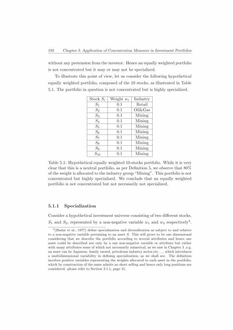
102 Chapter 5. Application of Concentration Measures in Investment Portfolios
without any pretension from the investor. Hence an equally weighted portfolio
is not concentrated but it may or may not be specialized.
To illustrate this point of view, let us consider the following hypothetical
equally weighted portfolio, composed of the 10 stocks, as illustrated in Table
5.1. The portfolio in question is not concentrated but is highly specialized.
Stock Si Weight wi Industry
S1 0.1 Retail
S2 0.1 Oil&Gas
S3 0.1 Mining
S4 0.1 Mining
S5 0.1 Mining
S6 0.1 Mining
S7 0.1 Mining
S8 0.1 Mining
S9 0.1 Mining
S10 0.1 Mining
Table 5.1: Hypothetical equally weighted 10-stocks portfolio. While it is veryclear that this is a neutral portfolio, as per Definition 5, we observe that 80%of the weight is allocated to the industry group “Mining”. This portfolio is notconcentrated but highly specialized. We conclude that an equally weightedportfolio is not concentrated but not necessarily not specialized.
5.1.1 Specialization
Consider a hypothetical investment universe consisting of two different stocks,
S1 and S2, represented by a non-negative variable w1 and w2 respectively4.
4(Hadar et al., 1977) define specialization and diversification as subject to and relativeto a non-negative variable pertaining to an asset S. This will prove to be one dimensionalconsidering that we describe the portfolio according to several attributes and hence oneasset could be described not only by a one non-negative variable or attribute but ratherwith many attributes some of which not necessarily numerical, as we saw in Chapter 3 ,e.g.an asset can be Japanese, family owned, petroleum industry sector,etc. . . , which introducesa multidimensional variability in defining specialization, as we shall see. The definitioninvolves positive variables representing the weights allocated to each asset in the portfolio,which by construction of the same admits no short selling and hence only long positions areconsidered. please refer to Section 3.1.1, page 41.

5.1. Portfolio Characteristics: Specialization and Concentration 103
Initially, a combination of those two assets creates a portfolio that can be
specialized if the weight of either one of the two stocks is 0 and the other
is 1, as discussed by Hadar et al. (1977). Defining a random portfolio P (k)
created from a combination of the two stocks as:
P (k) = kw1 + (1− k)w2 , with 0 ≤ k ≤ 1
The authors define a specialized portfolio as a portfolio with k = 0 or k = 1.
In the case where k = 0, P (k) = P (0) = w2, which is a portfolio specialized
in asset S2; in the case where k = 1, p(k) = P (1) = w1, which is a portfolio
specialized in asset S1. In the cited article, a portfolio is considered diversified
if and only if 0 < k < 1.
In our opinion, this definition is rather one dimensional in the sense that
it understates the attributes of an asset that we chose to consider as clearly
depicted in Figure 2.2 (Page 26). As apparent in this illustration, the spe-
cialization vector carries various dimensions and hence we need to specify a
different definition approach to specialization, other than the one used by
(Hadar et al., 1977).
To further illustrate our point in multidimensional specialization, consider
the example illustrated in Table 5.1. In fact the stocks Si included in this
portfolio, have the industry attribute as depicted, but also have the geograph-
ical location attribute as shown in the following Table 5.2, where an additional
attribute “Geographic Location” is added:

104 Chapter 5. Application of Concentration Measures in Investment Portfolios
Stock Si Weight wi Industry Location
S1 0.1 Retail USA
S2 0.1 Oil&Gas Japan
S3 0.1 Mining USA
S4 0.1 Mining USA
S5 0.1 Mining USA
S6 0.1 Mining USA
S7 0.1 Mining Japan
S8 0.1 Mining Japan
S9 0.1 Mining Japan
S10 0.1 Mining Japan
Table 5.2: Hypothetical equally weighted 10-stocks portfolio, showing twoattributes: Industry Group and Geographic Location. We observe that 80%of the weight is allocated to the industry group “Mining”, while the “Ge-ographic Location” weights are split 50-50 among USA and Japan. Thisportfolio is specialized in Mining and not specialized in Geographic location,or alternatively equally specialized in Japan and USA stocks, while being notconcentrated (i.e. equally weighted among all stocks).
Hence, Specialization is relative to the attributes of the stocks that the
analyst or the investor have chosen to include in the portfolio. The portfolio
can be specialized in one of these attributes while not specialized in another
one, or more specialized in one particular attribute and less specialized in
another one. We conclude that the term specialization must be preceded
by the attribute it measured: Geographic location Specialization , Industry
sector Specialization, etc..
Let us consider a second example in which we highlight the meaning of
specialization relative to multiple attributes.
Assume that we have a demonstration of 20,000 persons, 50 demonstra-
tors are picked at random. We want to describe this sample with respect to
some attributes chosen, or in other words, the specialization of this set of 50
demonstrators with respect to the following chosen attributes5 is required:
5The choice of attributes appears to be subjective in the present example and rathergeneric; attributes like gender seem to be an obvious choice with easy categories. But whenthe chosen attribute is age group an interval grouping is required or else a continuous scale

5.1. Portfolio Characteristics: Specialization and Concentration 105
• Gender: Male or Female. [40 M , 10 F]
• Education level: Illiterate, High school, University graduate. [16 I, 16
HS, 18 U]
• Age: Age group: 1,2,3,4. [5 G1, 5 G2, 20 G3, 20 G4]
• Region of origin: North, South, East or West. [9 N, 0 S, 0 E, 41 W]
We can calculate the specialization indexes of the demonstrators group
for each attribute chosen: specialization of gender, of educational level, of
age and of region. The result will be a set of indexes corresponding to the
attributes chosen. Note, however, in contrast to a portfolio, the concept of
“weight” is irrelevant as each protester is ultimately one person, one voice.
The weight distribution per element is 1 among 50, i.e. 1n = 1
50 . Therefore
the set of 50 demonstrators is a specialized set but its concentration is min-
imal, because it is equally distributed among its constituent elements. The
concentration of the demonstrators subset can be assessed by considering the
share in weight of each attribute subdivision. It is clear that the demon-
strators subset is specialized in Males, equally specialized in G3 and G4 age
groups, specialized in people from the Western region and not specialized in
any particular education level or equally specialized in all education levels.
We shall use the total weight per attribute to determine the specialization of
non overlapping set of elements ( investment portfolios in our case).
It is logical therefore, in an attempt to define a specialized portfolio, to
introduce along with the attributes of the asset its weight also. In the second
example above, the elements of the set under study (the demonstrators in the
sample chosen) are individuals and hence the concept of weight per element
is reduced to 1n = 1
50 as stated above. The examples used to illustrate the
specialization related to an attribute both represent an equally weighted al-
location. But even when the set is concentrated (i.e. not equally weighted)
or open scale of measurement is used. It is our choice to simplify the choice of intervalin this example and in the financial example that we discuss later in this chapter which issummarized in Tables 5.4 and 5.5 (pages 116 and 117), where the choice of the interval,albeit subjective, is not random but obeys a certain financial criteria that the analyst isinterested in exploring.

106 Chapter 5. Application of Concentration Measures in Investment Portfolios
the specialization measure can be proxied by the sum of weights (as in the
case of the portfolio in Table 5.2), or as the sum of individuals as in the case
of the demonstrators example.
On the other hand, we believe that the specialization of the portfolio
at hand must be related to the initial Investment Universe from which the
investor decided to choose his stocks. If the investor decided to choose his
stocks from the USA market, and if he chooses “Geographic Location” as an
attribute, it is very logical that the portfolio will include only stocks from
the USA and it is logical to say that the portfolio is highly specialized in
USA stocks, because the investor had no other geographic location to choose
from when he decided to invest in the USA market. The following example
illustrates graphically this particular situation:
Let U1 be an Investment Universe containing only USA companies, from
which we pick one stock S1, and let U2 be a different Investment Universe
containing European and Asian companies in equal proportion from which
we pick a stock S2. Let P1 and P2 be two different portfolios containing S1
and S2 respectively. Hence, P1 can contain a stock from the USA only and
P2 can contain a stock from either Asia or Europe, as shown in Figure 5.1.

5.1. Portfolio Characteristics: Specialization and Concentration 107
Figure 5.1: Both portfolios, P1 and P2 have the same Geographic Locationspecialization index (IP1 = IP2) since they both contain exactly one stock,while their initial Universes (U1 and U2) have different Geographic Locationspecialization level, because U1 is more specialized then U2 (IU1 > IU2).
What we can say about the Specialization of P1 and P2 related to the ge-
ographic location attribute is that both P1 and P2 contain only 1 geographic
attribute: P1 is specialized in USA stocks with a Specialization index6 IP1 = 1,
and P2 is also specialized in 1 geographic location (Asia or Europe). Thus,
both P1 and P2 have the same specialization level of 1. However, a struc-
tural difference exists between P1 and P2: P1’s Specialization index reflects
that this portfolio is specialized in one geographic location as well as P2’s,
P1 nevertheless reflects the exact specialization of its universe U1, namely
specialized in USA companies, while P2 introduces a different notation. In
fact, U2 is specialized in two geographic locations (EU and Asian companies)
while P2 is specialized in one single geographic location (in this case Asia). In
other words U2 is less specialized then P2 and this tells us a lot about P2. We
6We assume that the specialization index I is included in the interval I ∈ [0, 1] whereI = 0 represents the minimum specialization possible and I = 1 represents the maximumspecialization possible. Later in this chapter we will return to explore the meaning of eachvalue and we will specify the proper index to be used to represent the specialization levelin a portfolio.

108 Chapter 5. Application of Concentration Measures in Investment Portfolios
conclude that in order to be able to correctly describe the Specialization level
of a portfolio we must consider as well the specialization level of its initial
Universe to be able to compare. It is to be noted that we can describe P2
with sufficient relevance if we say “P2 is specialized in one geographic loca-
tion” but our description is more informative if we say “P2 is specialized in
one geographic location, increasing the specialization in this attribute com-
paring to its initial Universe U2”7. This concept of relative specialization
describes the specialization of a portfolio with respect to its investment uni-
verse. This becomes important when the investment strategy itself presents
constraints on the investors in form of investment principles or investment
compliance, like socially responsible investment, environment friendly invest-
ment or investment principle boycotting some sectors of the economy or even
some countries.
In other words, considering a Specialization index scalar I, the following
is a valid:
IU1 > IU2 ; while IP1 = IP2 = 1,
which describes P1 and P2 with respect to the attribute of geographic location,
as depicted in Figure 5.1. We can say the following with respect to the
attribute, “geographic location = USA stocks”:
IUSP1
= 1, and IUSP2
= 0 specialization level in USA stocks.
Similarly we can also say the following with respect to the attribute, “ge-
ographic location (Asia + EU) stocks”:
IAsia+EUP1
= 0, and IAsia+EUP2
= 1 related to the specialization level of P1
and P2 in (Asia + EU) stocks.
Specialization is therefore a descriptor relative to an attribute and it can
7This comparison between the Initial Investment Universe and the portfolio can be re-ferred to as the relative specialization. This relative attribute specialization remains howevertheoretical: In practice the investor does not start with a defined Investment Universe, butrather with a pretension on some markets. We are not therefore always sure what is theinitial universe that the investor started from. This is the case when we analyze an invest-ment portfolio without knowing the initial pretensions of the investors and hence without asufficient information and knowledge of the initial attributes he had in mind. In this case wecan define the attributes of analysis in a subjective manner and the relative specializationwill be irrelevant in this case.

5.1. Portfolio Characteristics: Specialization and Concentration 109
be also be measured as a relative specialization as compared to an initial Uni-
verse of population. The examples discussed in this present section will help
us define the Specialization in an investment portfolio.
Let P denote the portfolio with n stocks. The elements of P are the
stocks, Si, where i = 1, 2, 3, . . . , n.
Furthermore, let �p = A1, A2, . . . , Ak denote the vector of k desired attributes
Ak that the investor would like his portfolio to contain. Thus, the portfo-
lio contains n stocks each with k attributes. Each attribute Aj with j =
1, 2, 3, . . . , k has a size nj . Therefore the portfolio P is partitioned into k
attributes, and each attribute consists of nj subgroups. This subdivision is
illustrated in Table 5.5, page 117, which refers to our hypothetical portfolio
used for illustration throughout this thesis.
Definition 6. Specialization of a portfolio:
We define the absolute specialization of an investment portfolio within de-
fined attribute Ak as the measure of concentration of its consisting subgroups.
The portfolio will have as much specialization indexes Ik as it has attributes
AK . It is clear that the scalar being used in the measurement is the weight
of each stock, as subdivided into attributes and subgroups8.
The analyst can decide to analyze the specialization levels of various at-
tributes k, where each attribute specialization, that we denote Ik for now, is
such that Ik ∈ [0, 1]. Hence if our interval of measurement assumes a maxi-
mum value of 1, then a specialized portfolio is a portfolio such that Ik → 1.
The utilization of a concentration index to describe the portfolio at hand is
more eloquent and will give more relevant information when we compare the
concentration indexes of the same attribute k of both the Investment Universe
and the portfolio. This pairwise comparison gives a broader image, vis-a-vis
the attributes we have chosen k, on the description of the constituents of the
8It is clear from this discussion that the index of choice should have a decomposabilityfeature in order to show the concentration within each subgroup and between the subgroups.The Gini index, that we chose to measure specialization, has this particularity as shown inAppendix A.

110 Chapter 5. Application of Concentration Measures in Investment Portfolios
portfolio.
In this sense, the specialization vector that we established in Subsection
2.1.3 which is applied to an investment universe U to “extract” or filter out an
investment portfolio9 introduces the element of specialization in the resulting
filtered set. This specialization vector �p includes k = 4 filtering criteria, and
hence the corresponding sub-universe S = P (which is in our case the portfolio
that includes only those stocks that obey to the filtering criteria defined by the
investor) is a specialized portfolio. This specialization vector represents the
stock choice process (those stocks that the investor will invest his wealth in)
or Stage A we discussed earlier, which is the “specialization box” re-depicted
in Figure 5.2 below for ease of reference.
9�p={USA stocks, non-fincl Co., P/E ≥ 15, Debt/Assets ≤ 33.3%}

5.1. Portfolio Characteristics: Specialization and Concentration 111
Figure 5.2: Asset Allocation process. Please note the Specialization and theConcentration phases.
5.1.2 Concentration
As as shown in Figure 5.2 above, once the stock choice process or specializa-
tion is achieved, the investor moves to the wealth allocation stage, which is
the concentration stage. This stage consists of dividing the available wealth
among the stocks chosen. In theory, and assuming no short selling is allowed,
the allocated wealth proportion wi to stock i can take any value between 0
and 1, i.e. 0 ≤ wi ≤ 1 creating an infinite number of possible portfolios or
POS (portfolio opportunity sets), provided the budget constraint is always

112 Chapter 5. Application of Concentration Measures in Investment Portfolios
met. Some particular portfolios can be singled out like, for example:
1. A one stock portfolio which is the maximum concentration level possible
where all the wealth is placed in one single stock S: ws = 1 and wi = 0,
for all 1 < i < n with i = s.
2. An equally weighted portfolio or the neutral portfolio as defined in Defi-
nition 5 above, is a portfolio where the available wealth is divided equally
among all stocks n; hence wi =1n , ∀i = 1, 2, . . . , n. We can have only
one and unique equally weighted portfolio for a given choice of invest-
ment universe.
Definition 7. Concentration of a portfolio:
We define the concentration of a portfolio as the measure of inequality relative
to the weight allocation of the available wealth among the available stocks.
A portfolio where equal wealth is allocated to each and every stock chosen
initially by the investor, i.e. w1 = w2 = w3 = . . . wn = 1n , with no preference
of one stock over the other is called an equally weighted portfolio and hence
is the “minimum concentration portfolio”. This portfolio is equally weighted,
and by definition, this portfolio is not concentrated. A portfolio with all the
wealth invested in one single stock is, therefore, a maximum concentrated
portfolio.
The more the investor deviates from the 1/n wealth allocation strategy,
the more he invests in some stocks against the others within the n stocks uni-
verse. This will deviate his portfolio, consequently, from an equally weighted,
minimum concentration portfolio towards a maximum concentrated portfolio,
according to the weight allocation per stock 10.
10The concentration index of a portfolio tells us something very relevant about the in-vestor’s decision to choose this particular strategy. If he decides on an equally weightedallocation strategy, and hence his bet is on a neutral portfolio (see Definition 5) this tellsus that he does not have any particular preference of one stock over any other. This couldbe described as the investor’s pretension level. If he opts for a higher concentration levelin his portfolio this also tells us about his pretension concerning the chosen stocks over theothers. The pretension level will be discussed in more detail in Appendix B.

5.2. Specialization and Concentration Measurement in an Investment Portfolio 113
5.2 Specialization and Concentration Measurement
in an Investment Portfolio
For the purpose of illustration, we recall in this section the hypothetical ex-
ample we used in Chapter 2, which is a portfolio built up using the following
screening vector applied to a hypothetical investment universe:
�p1 = {Er > 7%, σ < 15%, PE > 12, USA+Jap, Phrm+Oil+Retl+Metl+Mining}
In the resulting portfolio P , there is a specialization in the US and Japanese
markets only, and a specialization in pharmaceutical and oil and retail and
metallurgical and mining companies, while excluding all other sectors. Be-
sides, among the chosen geographical and industrial sector specialization, the
filtering vector will admit only those companies with expected return Er > 7%
and whose standard deviation does not exceed 15% while also admitting only
those stocks whose Price earning ratio is above 12, as shown in the graphical
representation, Figure 5.3 and its corresponding Table 5.3 below.
< 15%
Figure 5.3: Graphical representation of the specialization vector �p1 = {Er >7%, σ < 15%, PE > 12, USA+ Jap, Phrm+Oil +Retl +Metl +Mining}.

114 Chapter 5. Application of Concentration Measures in Investment Portfolios
Si wi Eri, % σi, % P/Ei Location Industry
S1 0.07 14 8 12.5 Japan Pharma
S2 0.06 13.5 12 15 USA Oil-Gas
S3 0.07 16 9.5 13 Japan Oil-Gas
S4 0.08 11 14 14.5 Japan Pharma
S5 0.09 8 13 17 Japan Retail
S6 0.11 7.2 9 19 USA Pharma
S7 0.14 12 9 12.5 USA Metal
S8 0.18 15 14 14.7 Japan Metal
S9 0.09 12.5 14.5 19 Japan Mining
S10 0.11 9 13.9 15 USA Pharma
Table 5.3: Hypothetical 10-stocks portfolio resulting from the screening vec-tor: �p1 = {Er > 7%, σ < 15%, PE > 12, USA+Jap, Pharma+Oil+Retail+Metal +Mining}. This portfolio will be used to illustrate the usage of thetoolbox in this chapter.
Accordingly, the final Portfolio P shown in Figure 5.3, after applying the
screening filters �p can be expressed as the result of the intersection (and not
the subtraction) of each individual criteria-attribute within the chosen Invest-
ment universe and is represented as follows:
P = S(USA+Jap)∩S(Er>7%)∩σ < 15%∩S(P/E>12)∩S(Phrma+Oil+Retl+Metl+mining)
The reduction in number of included stocks can be very drastic according
to the number of filters and the level of cut–offs desired11.
11A typical vector of screens used to produce an Islamic Investment Universe out of theUSA market could reduce the initial Universe from 10,000 stocks to 1,500 eligible stocks, or

5.2. Specialization and Concentration Measurement in an Investment Portfolio 115
Our portfolio analysis methodology consists of identifying, therefore, the
screening attributes vector, and, after applying it to the selected Investment
Universe, we end up with the resulting “chosen” stocks to be included in the
investment portfolio as shown in Table 5.3. We then construct the weight-
attribute matrix, shown in Table 5.4, where we reflect the choices made in
the filtering vectors and map those choices against the resulting chosen stocks
Si. The weight-attribute matrix affected by the wealth distribution allocated
to each stock will result in the impact matrix, shown in Table 5.5, where the
impact of the weight vector on each attribute belonging to the filtering vector
is shown.
In summary, the hypothetical portfolio consists of 10 stocks. The chosen
attributes and their respective subgroups are:
Attribute Subgroup 1 Subgroup 2 Subgroup 3 Subgroup 4 Subgroup 5
Er > 7% ]7%, 10%[ [10%, 13%[ [13%,+[
σ < 15% ]0, 10%] ]10%, 15%[
PE > 12 ]12, 14[ [14, 16[ [16,+[
Location Japan USA
Industry Pharmaceutic Oil&Gas Retail Metallurgy Mining
It is interesting to note that the attributes and their subgroups are sub-
divided at the discretion of the analyst. For example the expected return
attribute Er was divided into 3 subgroups, as shown above, but it could as
well be divided into 2 subgroups or rather 4 subgroups. This subgrouping
within the attribute reflects the view of the analyst and his information re-
quirements within the target of his analysis.
a reduction in count by 85% (Chammas and Spronk, 2009).

116 Chapter 5. Application of Concentration Measures in Investment Portfolios
Er>
7%,E
r%
∈:σ<
15%,σ
%∈:
PE
>12
,PE
∈:Location
IndustrialSector
Si
wi
]7,1
0[
[10,1
3[
[13,+
[]0,1
0]
]10,1
5[
]12,1
4[
[14,1
6[
[16,+
[Jap
USA
Phr
Oil
Ret
Met
Mng
S1
0.07
11
11
1
S2
0.06
11
11
1
S3
0.07
11
11
1
S4
0.08
11
11
1
S5
0.09
11
11
1
S6
0.11
11
11
1
S7
0.14
11
11
1
S8
0.18
11
11
1
S9
0.09
11
11
1
S10
0.11
11
11
1
Tot
1.00
33
44
63
43
64
42
12
1
10
1010
1010
Tab
le5.4:Detailed
Weight-Criteriamatrix
ofahypotheticalspecializationvector�p1=
{Er>
7%,σ
<15
%,P
E>
12,U
SA+
Jap,P
harm
a+
Oil+
Retail+
Metal+
Mining}.
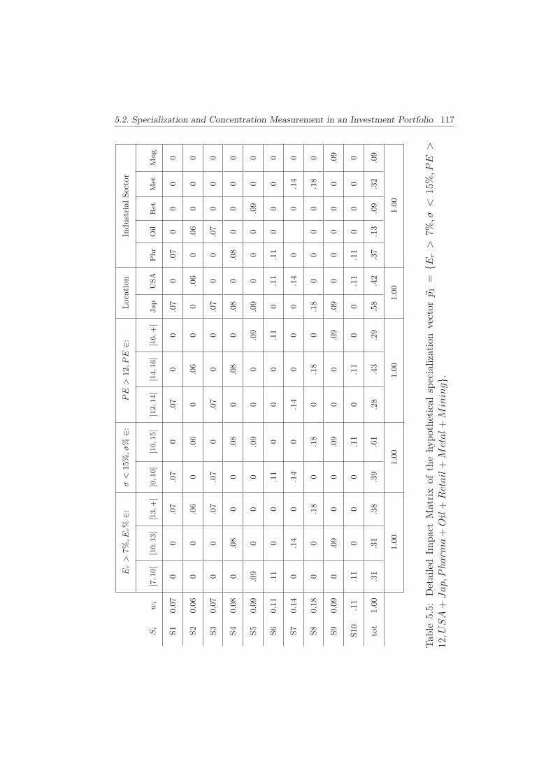
5.2. Specialization and Concentration Measurement in an Investment Portfolio 117E
r>
7%,E
r%
∈:σ<
15%,σ
%∈:
PE
>12,P
E∈:
Location
IndustrialSector
Si
wi
]7,1
0[
[10,1
3[
[13,+
[]0,1
0]
]10,1
5[
]12,1
4[
[14,1
6[
[16,+
[Jap
USA
Phr
Oil
Ret
Met
Mng
S1
0.07
00
.07
.07
0.07
00
.07
0.07
00
00
S2
0.06
00
.06
0.06
0.06
00
.06
0.06
00
0
S3
0.07
00
.07
.07
0.07
00
.07
00
.07
00
0
S4
0.08
0.08
00
.08
0.08
0.08
0.08
00
00
S5
0.09
.09
00
0.09
00
.09
.09
00
0.09
00
S6
0.11
.11
00
.11
00
0.11
0.11
.11
00
00
S7
0.14
0.14
0.14
0.14
00
0.14
00
.14
0
S8
0.18
00
.18
0.18
0.18
0.18
00
00
.18
0
S9
0.09
0.09
00
.09
00
.09
.09
00
00
0.09
S10
.11
.11
00
0.11
0.11
00
.11
.11
00
00
tot
1.00
.31
.31
.38
.39
.61
.28
.43
.29
.58
.42
.37
.13
.09
.32
.09
1.00
1.00
1.00
1.00
1.00
Tab
le5.5:Detailed
Impact
Matrix
ofthehypotheticalspecialization
vector�p1=
{Er>
7%,σ
<15
%,P
E>
12,U
SA+
Jap,P
harm
a+
Oil+
Retail+
Metal+
Mining}.

118 Chapter 5. Application of Concentration Measures in Investment Portfolios
5.2.1 Measuring Specialization: The Gini Index of each sub-
group and its total relative weight.
In a previous chapter, we have discussed the properties of the Gini index
and its adequacy to measure the specialization of a portfolio. Our definition
of specialization (Definition 6) refers to the concentration of the subgroups
related to the attributes of the securities included in a portfolio. In Appendix
A we present an extended view on the Gini index and its decomposition12.
The results of the formulas involved using the Gini index as a measure of
concentration13 are summarized in Table 5.6.
12The decomposition of the Gini index, as proposed by Dagum (1987) and detailed in Ap-pendix A, is applied when a population or group is divided into subpopulations or subgroupswith overlapping. In our case, a chosen portfolio attribute would divide it into subgroupsand we are interested in measuring the Gini or G index of each subgroup to describe thespecialization level related to this particular attribute. For this matter, G is decomposedinto three main components, so that G = Gw +Gnb +Gt as shown in Equation A.9a, andwhere:Gw is the weighted contribution to G of the Gini within the subgroup,Gnb is the net contribution to G of the Gini between subgroups,Gt is the contribution to G of the transvariation between subgroups,Ggb = Gnb +Gt is the gross contribution to G of the Gini between subgroups.We have also introduced the Gjnull which measures the G index within a subgroup tak-ing into consideration the null entries in the subgroup. If, within a portfolio of 10 stocks,the subgroup “pharmaceutical industries” is represented by four of the ten stocks, thenGPharmnull will be computed taking into consideration n = 10 and not n = 4, i.e. thenull entries are taken into consideration. This will enable us to compare specialization ofportfolios of different sizes (i.e. different n).
13We are measuring the specialization of the portfolio in one attribute using a concentra-tion measure, namely the Gini index and its decomposition. Hence the more concentrationindex a subgroup of an attribute exhibits, the more specialized the portfolio is in this at-tribute’s subgroup.

5.2. Specialization and Concentration Measurement in an Investment Portfolio 119
Index Er σ PE ratio Geo.Loc. Industry Gr
G, Gini index G = 0.186
Gjnull0.046 0.11 0.1 0.046 0.316
Ggb 0.134 0.092 0.129 0.1 0.166
Gnb 0.02 0.01 0.033 0.02 0.154
Gt 0.114 0.082 0.096 0.08 0.012
Gw 0.052 0.094 0.057 0.086 0.02
HHI HHI = 0.112
rHHI rHHI = 8.91
Table 5.6: Summary of the Gini decomposition formulas related to the hypo-thetical 10-stocks portfolio of our example and its HHI.
It is necessary to point out that, for each subgroup we considered and
within each subgroup, the sum of all partial weights within each subgroup is
always 1, i.e∑
pi = 1 where pi =nin . This means that no overlap between
the subgroup exists and hence we can conclude that, since no overlapping is
present, each attribute is a structural inequality factor, that is the partial
weights of its element constitute a basis for the calculation of the specializa-
tion. This method will be applied to our 500 stocks portfolio in Chapter 6
with satisfactory results.
To illustrate our point, please consider the following table, which analyzes
the attribute “industrial sector” related to our hypothetical portfolio:
id Industry Groups All Groups Oil- Gas Mining Retail Pharma Metal
1a Size of group 10 2 1 1 4 2
1b Total weight (qj) 1 0.130 0.09 0.09 0.37 0.32
1c Mean weight (μj) 0.1 0.065 0.09 0.09 .0925 0.16
1d Share of the group/Tot.Count (pj) 1 0.2 0.1 0.1 0.4 0.2
7 Gini Index (G = Gw +Gnb +Gt) 0.186
8 HHI 0.112 0.5 1 1 0.26 0.51
10 rHHI (reverse HHI) 8.91 1.99 1 1 3.86 1.97
11 rHHI/nj 0.891 0.99 1 1 0.96 0.98
Table 5.7: Industry group attribute: Gini (Specialization index) and HHI(Concentration index) toolbox output.
It is clear that the hypothetical portfolio at hand is specialized in Pharma-
ceuticals and metallurgy, by considering the relative weight of each industry.

120 Chapter 5. Application of Concentration Measures in Investment Portfolios
This will also be applied to a larger portfolio in Chapter 6.
5.2.2 Measuring Concentration: The HHI index.
The HHI measures the concentration level of the portfolio. The hypothetical
portfolio under study exhibits an HHI = 0.112 or a rHHI = 8.91. The min-
imum possible HHI in the case of a portfolio of 10 stocks is HHImin = 1n =
110 = 0.1 and hence a rHHI = 10. The portfolio at hand is not concentrated
at all and its HHI = 0.112 is very near the minimum concentration level
possible of 0.1. We can fairly conclude that the hypothetical portfolio under
study is not a concentrated portfolio. The rHHI = 8.91 � 9 shows that
the portfolio’s concentration level is identical to a 9 stock equally weighted
portfolio. This conclusion is corroborated by the similar derivations of the
HHI, where the corrected HHI or the cHHI = 0.0135 while the minimum
cHHI is equal to zero.
One important measure we derived is the rHHIn which is the per unit
concentration of a group. The lower this indicator is, the higher the absolute
concentration of the subgroup under study. In fact, since rHHI indicates
the equivalent number of equally weighted stocks which have a similar HHI
then the initial portfolio, then the per unit concentration rHHIn will allow the
analyst to compare the concentration of portfolios with different n.
Table ?? (rows 9 and 11) shows the minimum reached per unit rHHI
or rHHIn = 0.85 for the maximum reached cHHI = 0.06 for the subgroup
of PE ratio group between 14 and 16 or G2. This is the most concentrated
subgroup in the portfolio where 75% of the wealth allocated to this subgroup
is concentrated in 2 out of the 4 stocks available in this subgroup.
5.2.3 Description of the Hypothetical Investment Portfolio.
From the above discussion we can fairly say that our hypothetical portfolio
consisting of 10 stocks is not concentrated, with a rHHI = 8.91 i.e. it is
similar to a portfolio with almost nine equally weighted stocks.
As for the specialization of the portfolio in each of the attributes chosen,

5.3. Concluding remarks 121
we outline the following :
• Expected Return Attribute: The portfolio is not specialized in any sub-
group of the Expected return attribute.
• Standard Deviation Attribute: The portfolio is specialized in stocks
whose standard deviation σ, where 10% < σ < 15%.
• Price-Earning Ratio Attribute: A slight specialization of stocks whose
PE ratio is between 14 and 16 is shown.
• Geographic Location Attribute: The portfolio is specialized in stocks
from Japan more then stocks from the USA.
• Industry Groups attribute: The portfolio shows a specialization in phar-
maceutical industry stocks and metallurgy stocks among the other in-
dustries included in the portfolio. We also noted that, within the phar-
maceutics subgroup, their is no concentration of one stock against the
others since the weights within this subgroup is nearly evenly distributed
amongst the four stocks consisting of the pharmaceutics subgroup.
5.3 Concluding remarks
This chapter introduced the measurement of concentration and specialization
in an investment portfolio using HHI, Gini and the relative weight of each
element of the subgroups. The relative ease of computation makes these mea-
sures attractive and accessible for the user. We also note that the Gini index
decomposition which involves a pairwise comparison between the elements of
the portfolio, and a pairwise comparison between the elements of the sub-
groups, taken each two at a time, is not required nor necessary. It should
be noted that this decomposition can render the spreadsheet very bulky and
difficult to read when the portfolio subgroups become numerous, regardless
of the number of stocks in the portfolio. A further illustration in the next
chapter of our suggested method and measures will prove elegant, handy and
accessible to common desktop calculation tools.
122 Chapter 5. Application of Concentration Measures in Investment Portfolios
Within this context, several questions arise:
• Are these measures, as defined in this research, accepted or “liked” by an
investor? In other words, would an investor judge that, measuring the
concentration and specialization of his investment portfolio is a required
or necessary information for his investment? Consequently, are these
numbers and tables useful?
• Can the investor change the concentration and the specialization of
his portfolio using the technical insight that we are proposing? Can
the investor “fill in the gap” in his portfolio if the description of this
portfolio shows a certain specialization in some sectors against some
others that he wants to include in his portfolio?
• Eventually, will the description of the portfolio, vis-a-vis its concen-
tration and specialization be a useful addition to the usual return and
volatility information that is commonly used today in investment deci-
sions?
The application of our indexes to investment portfolios will be shown in
the next chapter. We will apply the HHI and the Gini index to measure the
concentration specialization of various 500 stocks portfolios and we will show
that the description provided by theses indexes is useful and relevant to the
investor and the financial market place at large.

Chapter 6
Concentration and
Specialization of the US
listed Stocks
6.1 Introduction
In previous chapters we have derived the formulas for measuring specializa-
tion and concentration in an investment portfolio as well as commented on
technical insights concerning these aforementioned measures when applied to
an investment portfolio. This resulted in tables that depict the results related
to our ten-stocks hypothetical portfolio. We chose the Hirschman-Herfindahl
index, HHI and its derivations to measure the concentration within a portfo-
lio of investment along with G , the Gini index. We also chose G to describe
the specialization of the portfolios.
In this chapter, we propose a numerical application of the toolbox, as
stated in the second part of research question 4.
We will apply our toolbox formulas to two series of quarterly portfolios1
1The quarterly portfolios that are formed for the purpose of our numerical study consistof the top 500 stocks listed at the end each quarter, i.e. last dealing day of month 3,6,9,12.The choice of these intervals is purely subjective and it could have been any other cut-offdate provided the intervals are equal.
123
124 Chapter 6. Concentration and Specialization of the US listed Stocks
composed of stocks listed in the United States. We will choose the top 500
stocks per capitalization in each period and we will form two portfolios. The
first one consists of a market-capitalization weighted portfolio Pmcap and the
second one an equally weighted portfolio Peq. Again, our approach to choose
only the top 500 stocks and not other number or to utilize the United States
listed stocks rather then the Japanese or the French listed stock is purely
subjective. We believe that our choice was mainly oriented by the ease of ob-
taining the data and the abundance of listed companies in the United States.
The choice to include 500 top market capitalization stocks in a given trading
day was to include as many stocks as possible by the limited computational
resources we have available.
Throughout the time interval of our consideration, from January 1993
until September 2013 included, Our analysis will be two-fold:
• Describe the trends and the variation over time of the concentration and
the specialization of the quarterly portfolios described in the methodol-
ogy section, and
• Describe the concentration and the specialization of equally weighted
and market capitalization portfolios of three particular quarters that we
believe are outstanding examples of the methodology we wish to convey
in this thesis. This means that we will study thoroughly 6 portfolios
pertaining to 3 different quarters and constructed in two different ways.
Our data consists of around 82 consecutive quarters spanning over 21 years
of American Stock exchange listed stocks, as described in the following sub-
section.
6.1.1 Data Description and Methodology.
The data was downloaded from the CRSP/COMPUSTAT database. It
comprises stocks listed in the United States from the date : January 1993 until
September 2013 included. We downloaded monthly end-of-the-month closing
prices along with the basic fundamentals listed, mainly capitalization values,

6.1. Introduction 125
price in base currency, number of shares, trading volume, industry identifi-
cation code, price in base currency, exchange rate, local currency, country
identification, book value-to-price ratio along with the usual stock identifiers
like GIND code and CUSIP code. The data was analyzed and its robustness
was tested. Some minor corrections were made to eliminate obvious stray val-
ues or to extrapolate between previous and next month to replace a monthly
fundamental which is missing. In total only 25 minor corrections were made.
The data is robust and the results we obtained look solid and consistent with
previous published data on returns and volatility.
For the purpose of our analysis, the data we used represents the USA
stock exchange market from Q1 of 1993 inclusive until Q3 of 2013 inclusive,
for a total of 82 quarters data. Therefore our study includes 82 quarterly
portfolios with market capitalization weights allocation Pcap and 82 quarterly
portfolios with equal weights allocation Peq.
On every end of month, we calculated the market capitalization of each
stock and sorted the results by descending order. Every month, the first 500
stocks were included in our dataset.
We choose the attribute of “industry group” to conduct our analysis of
concentration and specialization. We have detected 44 different industry sub-
groups that are specified by the database2 we downloaded. We have noted
the creation of new subgroups that were not existing at the initial date of
our data but were introduced later like the subgroup “REIT” (Real Estate
Investment Trust.) or “Cellular and Wireless”.
2The complete list of industry subgroups is the following: Agriculture, food, beverage;Beer, liquor, and tobacco; Basic minerals and metals; Oil and coal resources; Integratedoil companies; Oil drilling and services; Oil distribution; Construction materials; Forestproducts, paper; Construction, home-building; Chemicals, rubber; Metal products, machin-ery; Instruments; Mainframe & minicomputers; Photo-optical, micros, office machinery;Textiles and apparel; Drugs & pharmaceuticals; Soaps & cosmetics; Furniture, householditems; Consumer durables; Cars and trucks; Commercial aircraft, components; Govt. air-craft & defense; Land and water transportation; Airlines; Electric utilities; Gas and otherpublic utilities; Communications utilities; Publishing, broadcasting, cinema; Restaurants,hotels, theaters; Retail; Health care & hospital; Information, services; Real estate develop-ment; Financial investments; Banks & credit institutions; Miscellaneous finance; Insurance;Biotechnology; Software; Cellular & wireless; IT hardware; Reits; Wholesale; Trading com-pany.

126 Chapter 6. Concentration and Specialization of the US listed Stocks
The Methodology The analysis is two-fold and consists first of an
overview of the 21 years period of quarterly portfolios that we will create,
with respect to the variations and trends in their respective concentration and
specialization. Second, the analysis will focus of 3 particular quarters that
we will choose which exhibit maximum and relative minimum concentrations,
describing each particular portfolio with respect to its concentration and spe-
cialization. The purpose of the first analysis is to observe the variations of
the portfolios’ concentration during the observed period and to compare the
variation of the equally weighted to the cap weighted strategy. The purpose
of the second analysis is to explain the observed remarkable or important vari-
ations (drastic jumps or declines in concentration, absolute extreme values)
and try to examine their particular specialization. It is worth noting that the
analysis will not attempt to explain the reasons behind the variations or the
plausible causes of the change in specialization.
We are particularly interested in exploring and describing equally weighted
portfolios and market capitalization weighted portfolios in function of their
concentration and specialization. It is worth noting that we have decided to
choose the top market capitalization 500 stocks from the available investment
universe for ease of data manipulation and for maximum relevance to our
analysis.
Accordingly, two quarterly portfolios are first created as follows:
(a) A cap-weighted portfolio, Pcap, comprising the first 500 market capital-
ization values, calculated at the end of each month, where the weight
wi for Stock Si, i = 1, 2, 3, . . . , 500 is equal to:
wi =Capi∑5001 Capi
where Capi is the market capitalization of stock Si during the period in
consideration.
(b) An equally weighted portfolio, Peq, comprising the first 500 market cap-
italization values, calculated at the end of each month, where the weight

6.1. Introduction 127
wi for Stock Si, i = 1, 2, 3, . . . , 500 is equal to:
w1 = w2 = · · · = wi =1
500= 0.002.
In both portfolios we assume no short selling is allowed and hence the budget
constraint in both portfolios,∑500
i=1wi = 1, is always met.
We will consider the attribute of “industry group” to subdivide our port-
folios into subgroups, one subgroup being the industry group: for example
subgroups like “Furniture, Household Items”, “Communication Utilities”, or
“Soaps & Cosmetics” are actual examples of subgroups in our portfolios3.
We will then calculate for each quarterly portfolio the concentration and
the specialization measures, as suggested in Chapter 5. We will compile the
results in tables and use them to describe the portfolios at hand. We will
show that using the concentration and specialization measure is useful and
gives the investor an additional insight on his investment, with no estimation
errors involved.
The results we obtained show clear patterns of concentration and special-
ization over time, and we will highlight some important dates and describe
the portfolio around these dates. We will show that the specialization of the
portfolio changes over time and that the investor is capable of detecting these
changes and taking the decision to modify the content of the portfolio with
respect to its concentration and specialization.
Additionally, our results will give the investor an insight on how the econ-
omy is changing over time, as well as an insight to the state of his portfolio
at a particular time of observation (in our case quarterly observations).
The methodology of using the concentration and specialization measure
to describe an investment portfolio comprises the following calculation levels:
1. At the individual stock level: Given the 500 stocks of the portfolio,
each with its weight wi, we will calculate the HHI and G at the level of
3It is worth noting that, due to the initial constraint we have imposed by including onlythe top 500 market capitalization stocks in both the Pcap and Peq, some industry subgroupswill eventually not be represented in some quarterly portfolios because they fall outside thetop 500 stocks chosen.

128 Chapter 6. Concentration and Specialization of the US listed Stocks
the individual weights. In this case the number of entries in the universe
is n = 500. This process is applied to all 82 quarterly portfolios.
2. At the weight of industry sectors level: Given a quarterly portfolio,
we observe that its 500 stocks are clustered in the possible 44 industry
subgroups available in the initial data. We will calculate the HHI and
G of the sum of weight of the stocks per each subgroup, i.e. the sum of
weights per industry subgroup or cluster. This will give us the industry
concentration of the portfolio. In this case the number of entries in the
universe is maximum nmax = 44, corresponding to the total number of
industries available in the portfolio. This process is also applied to all
the 82 quarterly portfolios.
3. At the subgroup level: the 500 stocks, clustered in the available
44 industries are then considered at each subgroup level (each indus-
try apart). We will calculate within each subgroup the concentration
level and we shall compare the weights of individual industry levels to
determine the specialization of the portfolio.
4. At 3 particular portfolios chosen after analyzing the 82 quarterly
portfolios we created as per the first 3 steps here-above, three particular
portfolios will be considered. The portfolio of absolute maximum con-
centration, the portfolio of relative minimum concentration occurring
directly after it and the portfolio of absolute minimum concentration,
within the time bracket of our study. The subsequent tables and figures
will show that these portfolios are 2000 Q1 (the maximum concentra-
tion portfolio), 2005 Q2 (a subsequent relative minimum concentration
portfolio) and 1994 Q3 (an absolute minimum concentration portfolio).
These special portfolios are highlighted with bracket selection on Figure
6.4 and all major graphs in this chapter.
6.2. Results: Concentration and Specialization of Peq and Pcap. 129
6.2 Results: Concentration and Specialization of
Peq and Pcap.
It follows that the results obtained are divided into two parts: Part I will
describe the evolution and trend of concentration and specialization from
1993 until 2013 in the United States stock market and, Part II will describe
the concentration and specialization of the 3 particular portfolios chosen, as
summarized in Table 6.1. We shall point out to some particular and specific
economic and market events and crisis that occurred within the time span
of the particular 3 portfolios we are considering, to further show that our
approach offers a particular insight into the investment situation per se, with-
out establishing any inferential conclusion or a causal relationship between
the concentration level and the economic event.
Our approach provides a different angle to look at the market and its
dynamics, and this view focuses on concentration and specialization. We
describe the evolution and trends of concentration and specialization of Peq
and Pcap throughout the entire period of data available (i.e. from 1993 Q1 to
2013 Q3 both inclusive). In this section we will explore the results we obtained
and present an in-depth commentary on the same in view of i) describing the
portfolios at hand, ii)use the concentration and specialization measures as a
detection tool for possible market patterns or tendencies that will eventually
help in investment decision making and iii) propose our measures as a possible
foundation to monitor investment portfolios4. Table 6.1 shows the content of
the results Part I and Part II for clarity.
4The present section contains graphs whose labels will follow the following abbreviations:“Gini eq stk” stands for The Gini index for Peq at the stock level. “Gini cap stk” standsfor the Gini index for Pcap at the stock level. “Gini eq ind” stands for the Gini index forPeq at the industry cluster level and “Gini cap ind” stands for the Gini index for Pcap atthe industry cluster level. Similarly for “HHI eq stk” which represents the HHI index forPeq at the stock level.

130 Chapter 6. Concentration and Specialization of the US listed Stocks
PART I PART IIAll Portfolios 3 Special Portfolios
Measurement Pcap Peq Pcap Peq Pcap Peq Pcap Peq
Concentration: at Stock Level x x x x x x x x
Concentration: at Industry Level x x x x x x x x
Specialization: at Industry Level x x x x x x x x
Table 6.1: Mapping of the content of Part I and II analysis that the resultswill reflect in this subsection
6.2.1 Results Part I: Variation of Concentration of Pcap and
Peq.
When the equally weighted portfolio, Peq is considered, some obvious results
can be deduced intuitively, even prior to calculating its concentration levels:
• First, by virtue of its design, an equally weighted portfolio exhibits no
concentration at the level of individual stocks included. Each stock of
the 500 has a weight of:
w1 = w2 = · · · = w500 =1
500 = 0.002, obeying to the budget constraint∑500
i=1wi = 1.
This leads us to deduce that HHIPeq = 1n = 0.002, and
GPeq = 0
• Second,When considering the industry groups clustering, the equally
weighted portfolio is not at its minimum concentration level. The 500
stocks are clustered among 44 industry groups, and hence this clustering
is not equally weighted. Our Table 6.4 below will show the values of the
industry clustering concentration for each quarterly portfolio.
• Third, It is intuitive to observe that the specialization of the equally
weighted portfolio follows the concentration of the industry clusters. In
fact, since the individual weights are all equal to 0.002, hence the total
weight per cluster of industries is:
windj = 0.002 × Sj , where Sj is the number of stocks included in the
industry cluster j.

6.2. Results: Concentration and Specialization of Peq and Pcap. 131
It follows that the bigger the Sj of a given industry cluster, the more
specialized the portfolio in this particular cluster of industry j. We
can generalize this conclusion to any given attribute m, where, for an
equally weighted portfolio, the count of the individual stocks clustered
in an attribute m, defined by the investor, represents the specialization
of the portfolio in this particular attribute.
Concentration measures of Peq ands Pcap at the level of individual
weights of stocks.
As discussed earlier, the HHI and the Gini index were measured at the
500 stocks constituting each portfolio, at quarterly intervals. The results
are depicted in Figure 6.1. The straight line confounded with the x-axis,
represents a value of Gini = 0 for the equally weighted portfolio, whereas its
corresponding HHI = 0.002 is depicted in the red dashed line directly above
it. Please note that HHI is plotted against the secondary axis to the right
of the figure.

132 Chapter 6. Concentration and Specialization of the US listed Stocks
Figure 6.1: Gini and HHI indexes of quarterly portfolios Peq and Pcap con-sisting of 500 stocks each. Peq concentrations measures are represented by astraight line ( Gini= 0 and HHI = 1
n = 1500 = 0.002). Note that HHI is
plotted against the secondary axis to the right of the graph.
The concentration of the Pcap portfolio is not constant over time. We can
observe some local peaks, namely during the year 2000 where a Gmax = 0.6349
was reached in Q2 of 2000 (corresponding to HHI = 0.0096), followed by a
steady decline in concentration and then another prominent peak in the last
quarter of 2008 and first half of 2009.

6.2. Results: Concentration and Specialization of Peq and Pcap. 133
Pcapstk -Top 10 (max) values Pcapstk -Bottom 10 (min) values
Quarter Gini HHI rHHI Quarter Gini HHI rHHI
2000 Q2 0.634 0.0096 103 1993 Q3 0.487 0.0053 186
2000 Q1 0.625 0.0098 101 1993 Q4 0.489 0.0054 185
2000 Q3 0.609 0.0086 115 1993 Q2 0.499 0.0056 176
1999 Q4 0.624 0.0098 101 1993 Q1 0.501 0.0057 174
1999 Q1 0.618 0.0087 114 1994 Q2 0.497 0.0054 183
1999 Q3 0.617 0.0090 110 1994 Q1 0.489 0.0054 183
2001 Q4 0.614 0.0091 109 1994 Q3 0.498 0.0054 182
2001 Q3 0.625 0.0092 107 1994 Q4 0.507 0.0057 175
2001 Q1 0.608 0.0085 116 1995 Q1 0.505 0.0056 177
2001 Q2 0.607 0.0092 107 1995 Q3 0.509 0.0056 175
Table 6.2: Summary of the top and bottom 10 concentration values, measuredat the stocks level, related to Pcap.
It is noticeable that the rHHI, representing an equivalent number of
equally weighted stocks portfolio varies between rHHI = 101 and rHHI =
186 out of the 500 stocks of the quarterly portfolios. This indicates a fairly
high level of concentration in the market capitalization portfolio Pcap, as seen
in Figure 6.2
Figure 6.2: rHHI for both Peq and Pcap.
The rHHI of Pcap, during the observed period of 82 quarters, varied
between 101 and 186. The mean value of rHHI is 139 and the median value
is 136. However the histogram of rHHI reveals a tendency towards more
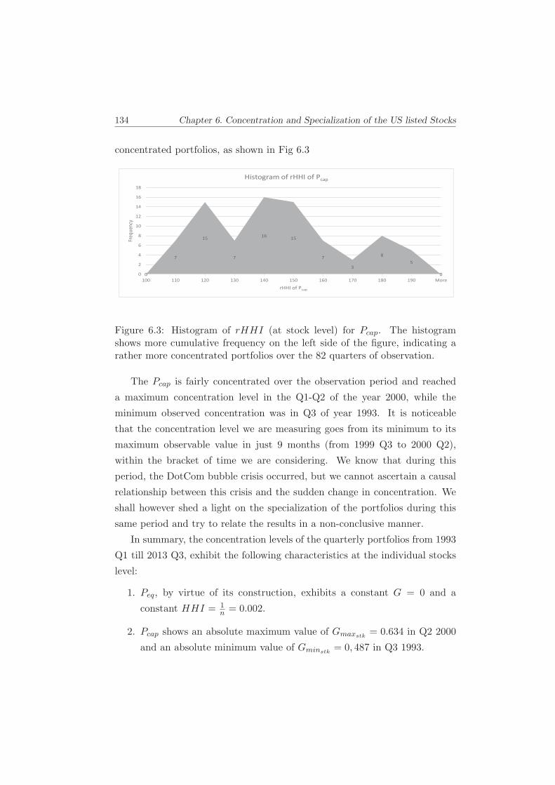
134 Chapter 6. Concentration and Specialization of the US listed Stocks
concentrated portfolios, as shown in Fig 6.3
Figure 6.3: Histogram of rHHI (at stock level) for Pcap. The histogramshows more cumulative frequency on the left side of the figure, indicating arather more concentrated portfolios over the 82 quarters of observation.
The Pcap is fairly concentrated over the observation period and reached
a maximum concentration level in the Q1-Q2 of the year 2000, while the
minimum observed concentration was in Q3 of year 1993. It is noticeable
that the concentration level we are measuring goes from its minimum to its
maximum observable value in just 9 months (from 1999 Q3 to 2000 Q2),
within the bracket of time we are considering. We know that during this
period, the DotCom bubble crisis occurred, but we cannot ascertain a causal
relationship between this crisis and the sudden change in concentration. We
shall however shed a light on the specialization of the portfolios during this
same period and try to relate the results in a non-conclusive manner.
In summary, the concentration levels of the quarterly portfolios from 1993
Q1 till 2013 Q3, exhibit the following characteristics at the individual stocks
level:
1. Peq, by virtue of its construction, exhibits a constant G = 0 and a
constant HHI = 1n = 0.002.
2. Pcap shows an absolute maximum value of Gmaxstk= 0.634 in Q2 2000
and an absolute minimum value of Gminstk= 0, 487 in Q3 1993.

6.2. Results: Concentration and Specialization of Peq and Pcap. 135
3. In terms of rHHI, the 500 stocks included in Pcap did not exceed the
value of rHHImaxstk= 186 in 1993 Q3 and an absolute minimum value
of rHHIminstk= 101 both in 1999 Q4 and 2000 Q1, where the concen-
tration reached its maximum. This means that, at its most concentrated
level, the 2000 Q1 portfolio was equivalent to a virtual portfolio of only
101 stocks out of the 500 available (1:5 compression). At its best, the
least concentrated portfolio, at the start of the observation period, is
represented by a virtual equivalent portfolio of 187 stocks out of the 500
available (approximately 2:5 compression). It is to be noted that the Peq
portfolios’ rHHI = 500 throughout the entire period of observation, as
shown in Figure 6.2.
Concentration measures of Peq ands Pcap at the level of industry
sectors.
When we consider clustering the stocks of each portfolio, namely of Pcap
and Peq in the stocks’ respective industry subgroup, we obtain a different
levels of concentration, and the equally weighted portfolio starts exhibiting
concentration levels different from the HHImin = 0.002 and Gmin = 0. This
is due to the fact that we have 500 stocks in the portfolio but only 44 industry
sectors related to these stocks. Therefore, when we consider the concentration
level of the portfolios under study with respect to the industry sectors we will
obtain a different set of concentration levels, as is apparent in Figure 6.4.
The graph in Figure 6.4 shows the same peak in concentration at around
the period from 1999 Q3 to 2000 Q2 that was singled out in the previous
subsection above, but with a sharper slope. if we plot in the same graph
the concentration measures of both portfolios with respect to the individual
stocks (Figure 6.1) and industry clusters (Figure 6.4), we are able to compare
the respective concentration values per quarter, as shown in Figure 6.5.

136 Chapter 6. Concentration and Specialization of the US listed Stocks
Figure 6.4: The Industry cluster’s Gini and HHI indexes of quarterly port-folios Peq and Pcap consisting of 500 stocks each and clustered around 44industry sectors. Note that HHI is in dotted lines and is plotted againstthe secondary axis to the right of the graph. The brackets indicate the 3portfolios selected for analysis in PART II of the results.
Pcapind-Top 10 (max) values Pcapind
-Bottom 10 (min) values
Quarter Gini HHI rHHI Quarter Gini HHI rHHI
2000 Q1 0.665 0.0755 13 1994 Q3 0.482 0.0424 23
2000 Q2 0.653 0.0715 13 1994 Q4 0.483 0.0419 23
1999 Q4 0.642 0.0690 14 1993 Q4 0.484 0.0433 23
2000 Q3 0.627 0.0627 15 1994 Q1 0.486 0.0427 23
2001 Q2 0.604 0.0618 16 1994 Q2 0.487 0.0432 23
1999 Q3 0.603 0.0598 16 2005 Q3 0.488 0.0418 23
2001 Q3 0.602 0.0606 16 2005 Q4 0.488 0.0421 23
2001 Q1 0.601 0.0601 16 2012 Q4 0.488 0.0416 24
2001 Q4 0.597 0.0587 17 1995 Q1 0.491 0.0427 23
1999 Q1 0.593 0.0587 17 2013 Q1 0.492 0.0421 23
Table 6.3: Summary of the top and bottom 10 concentration values, measuredat the industry clusters level, related to Pcap.

6.2. Results: Concentration and Specialization of Peq and Pcap. 137
Peqind-Top 10 (max) values Peqind
-Bottom 10 (min) values
Quarter Gini HHI rHHI Quarter Gini HHI rHHI
2000 Q1 0.542 0.0524 19 2005 Q2 0.414 0.0375 26
2000 Q2 0.540 0.0519 19 2005 Q3 0.417 0.0370 26
2000 Q3 0.538 0.0506 19 2005 Q1 0.419 0.0378 26
1999 Q4 0.530 0.0507 19 2006 Q2 0.424 0.0367 27
1999 Q3 0.505 0.0465 21 2005 Q4 0.427 0.0380 26
1999 Q1 0.502 0.0460 21 2006 Q4 0.429 0.0370 26
1999 Q2 0.499 0.0458 21 2006 Q1 0.430 0.0377 26
2000 Q4 0.498 0.0449 22 2004 Q3 0.432 0.0396 25
1998 Q4 0.494 0.0460 21 2004 Q4 0.432 0.0390 25
1995 Q4 0.491 0.0454 21 2008 Q3 0.434 0.0368 27
Table 6.4: Summary of the top and bottom 10 concentration values, measuredat the industry clusters level, related to Peq.
We observe that the industry clusters’ concentration is usually less then
that of the individual stocks except in the periods of 1993 Q4 (one quarter
only) and, more notoriously, in the period between 1993 Q3 and 2000 Q2.
In this latter period, the industry clusters concentration measure peaks to
G = 0.665 in 2000 Q3, which is the highest attainable concentration during
the period under study. The concentration measure for the Peq at the industry
level (line labeled ‘Gini eq ind’ in Figure 6.5)is always less the Pcap at all time
during the period under study.

138 Chapter 6. Concentration and Specialization of the US listed Stocks
Figure 6.5: A comparative graph of Gini concentration at the levels of bothIndustry cluster’s and individual stocks. Note that during the period of 1999Q3 to 2000 Q2 we observe that the industry clusters’ concentration is higherthen the individual stocks concentration.
In summary, the concentration levels of the quarterly portfolios from 1993
Q1 till 2013 Q3, exhibit the following characteristics at the industry clusters
level:
1. Peqindexhibits pronounced concentration levels, specially around the
same period we detected earlier, i.e. 1999 Q3,Q4 till 2000 Q3. It is to
be noted that GPeqindreaches 0.542 at its maximum value compared to
GPcapindmaximum of 0.665, as shown in tables 6.3 and 6.4.This corre-
sponds to a rHHI of 19 and 13 respectively, for a compression level
of 4:10 against 2.8:10 respectively. The market cap portfolios are more
concentrated then the equally weighted portfolios when the industry
clusters are considered.
2. As seen in Figure 6.4, a relative minimum or ‘dip’ in the Gini curves
is noticeable at around 2005 Q2 and Q3, where GPeqindreaches 0.414
(rHHI = 26) at its absolute minimum value compared to GPcapind
relative minimum of 0.488 corresponding to a rHHI = 23. In our
PART II analysis, we will analyze this portfolio among two others.
3. In Figure 6.5 we observe that the curve of GPcapind(in solid line) is

6.2. Results: Concentration and Specialization of Peq and Pcap. 139
always below the curve of GPcapstk(in dotted line) except in the short
period of 1999 Q3 to 2000 Q2. The individual stocks concentration
exhibiting a higher concentration level is counter intuitive. In fact, the
intuitive rationale is that the more scattered a sample is the less concen-
trated it is, and the more clustered and grouped the more concentrated
it is. However, in the case of portfolio concentration, the clustering or
grouping of individual stocks around their respective industry sector will
relatively smooth out the differences between individual stocks weights,
in the absence of an absolute single industry class heavy weight. This is
further corroborated when we observe the GPeqind(in double line) which
falls below both above mentioned curves. 2000 Q1 will be considered
individually in the PART II analysis to further explore its specialization
particularity.
Specialization of Pcap and Peq at the level of industry sectors.
Pcap The graphs and figures of this paragraph are depicted in Appendix C,
Page 185 for better clarity. Each graph will be plotted on a separate
page for ease of reading.
In order to determine the specialization in industry sectors and its varia-
tion over all the 83 quarters’ portfolios that we formed , we will consider
the ranking in weight of each industry sector in each portfolio (i.e. in
each quarter). This ranking of each industry is not constant over time
and will vary from quarter to other and hence the specialization of the
portfolios is not the same and will accordingly vary from a quarter to
another.
The ranking involves the 43 industries and hence one industry will be
ranked first, being the heaviest in a given portfolio among the 43 in-
dustry sectors existing. So it is natural to conclude that the portfolio is
not only specialized in the first in rank industry sector, but also among
other following industry sectors as well. The issue is where to draw
the line and decide that we shall consider the first 5 sectors or the first

140 Chapter 6. Concentration and Specialization of the US listed Stocks
10 in weight ranking. What could be a consistent criteria to follow
in order to produce comparative and consistent results over different
portfolios? One possible criteria is to use the Pareto 80-20 principle,
drawing the line at the 20% of the industry sectors (i.e. after the first
43 × 0.2 = 8.6,the 8th or 9th ranked industry). However, the idea of
using Pareto rule with 80% of the weight concentrated in 20% of the
industry sectors seems to be far fetched. In fact, in a well planned
and scientifically allocated portfolio, diversification will impose a lower
weight percentage at the 20% cut-off line for which we decided to opt
out of the Pareto rule.
Nevertheless, and in order to determine an intuitive approach to the
minimum or adequate number of industry sectors determining the spe-
cialization of the portfolio (the cut-off line), we drew the following
graph, represented in Figure 6.6, depicting the number of industries
that achieve a 10, 25, 50, 75 and 90% of the total weight of the portfo-
lio.

6.2. Results: Concentration and Specialization of Peq and Pcap. 141
0123456789
101112131415161718192021222324252627282930
1993
0319
9306
1993
0919
9312
1994
0319
9406
1994
0919
9412
1995
0319
9506
1995
0919
9512
1996
0319
9606
1996
0919
9612
1997
0319
9706
1997
0919
9712
1998
0319
9806
1998
0919
9812
1999
0319
9906
1999
0919
9912
2000
0320
0006
2000
0920
0012
2001
0320
0106
2001
0920
0112
2002
0320
0206
2002
0920
0212
2003
0320
0306
2003
0920
0312
2004
0320
0406
2004
0920
0412
2005
0320
0506
2005
0920
0512
2006
0320
0606
2006
0920
0612
2007
0320
0706
2007
0920
0712
2008
0320
0806
2008
0920
0812
2009
0320
0906
2009
0920
0912
2010
0320
1006
2010
0920
1012
2011
0320
1106
2011
0920
1112
2012
0320
1206
2012
0920
1212
2013
0320
1306
2013
09
Num
ber o
f indu
stries
Pcap Quarterly Portfolios
Pcap. Number of industries acheiving x% of weight
10%
25%
50%
75%
90%
90% of
25% of weight
50% of weight
75% of weight
10% of weight
1999
119
991
1999
119
9912222
2000
020
000
2000
020
0003333
2000
020
000
2000
020
0006666
2005
020
050
2005
020
050
2005
03333320
050
2005
020
050666
2005
020
050
2005
020
0509999
1993
119
931
1993
199
3222
1994
019
940
1994
033319
940
1994
019
940
1994
019
94066666
Figure 6.6: Number of industry sectors achieving 10,25,50,75 and 90% of totalweight of Pcap. Note also the brackets indicating the special portfolios thatwill be considered later.
The green curve in Figure 6.6 ( third curve from above) represents
50% of the weights related to the first top 9 ranked industry sectors.
This green curve represents the 80-20 Pareto principle since 80-20 of
weights-sectors is indeed 50% of the weight represented by 9 sectors.
We think that choosing the first 7 to 9 industry sectors to decide on
the specialization of the portfolio is fair and will reflect the purpose of
our study, knowing that the first 7 to 9 top ranked industry sectors are
representative of at least 50% of the total weight of the portfolio.
Adopting the top ranked industries by weight to determine the spe-
cialization of the portfolio can be misleading or, to say the least, in-
complete. Mathematically, the top m industries by weight could be all
equally weighted or nearly equally weighted, and hence the conclusion
that the portfolio is specialized in any of these top m industries is not
conclusively correct. We must explore the dispersion of the weights of
industries within the top m industries and hence, a Gini index of the

142 Chapter 6. Concentration and Specialization of the US listed Stocks
higher ranking industries must be calculated and the degree of special-
ization in a given industry rather then in others can be correctly as-
sessed. We shall explore this aspect of the specialization in more details
later in this chapter.
Figure 6.7 comprises four stacked individual graphs, dividing the 83
portfolios under study into four groups for ease of reading. Each graph
is also depicted alone in Appendix C for detailed reading. Please refer
to Figures C.2, C.3, C.4 and C.5 in Pages 188 to 191.
From this stacked graph we realize that the “Ind 28” is more often
ranked among the first 3 industries through all the period under study.
Table 6.5 summarizes the top industries in each period under study.
We observe the exit of “ Agriculture, Foods, Beverages”” in Period 2, 3
and 4. In fact, Figure C.2 shows that this industry exits from the top
ranked sectors in 1998 Q3. A complete histogram of the frequencies of
rank per each industry is depicted in Figures C.6 to C.14, Pages 192 to
200. The histograms and the relative frequency plots show clearly the
“history” of the rank frequency of each industry subgroup throughout
the portfolios under studies. These bar graphed histograms are very
useful when studying the rank of a given industry throughout a panel
of time portfolios. For example, if we consider “Ind 7” in Figure C.6
we can see that this industry (Oil Distribution) has never been ranked
among the top 10, and the best ranking reached is Rank 20, and the
most frequent rank occupied was rank 41. Furthermore, considering
“Ind 17” (Drugs and Pharmaceuticals) in Fig C.10, Page 196, we can
see that the histogram shows that this industry has always been one of
top 10 industries, during the period under study, mostly occupying rank
3, 4 or 5, as shown, while “Ind 36”, (Banks and Credit Institutions) in
Figure C.13, shows that this industry sector has almost always occupied
the first, second or third rank.

6.2. Results: Concentration and Specialization of Peq and Pcap. 143
Period 1 Period 2 Period 3 Period 4
From 1993 Q1 1999 Q1 2005 Q1 2011 Q1
Till 1998 Q4 2004 Q4 2010 Q4 2013 Q3
Rank 1 CommunicationUtilities
CommunicationUtilities
Banks &CreditInstit.
Banks &CreditInstit.
Rank 2 Banks &CreditInstit.
Banks &CreditInstit.
Retail Retail
Rank 3 Retail Retail Software Drugs & Phar-maceutics
Rank 4 Drugs & Phar-maceutics
Drugs & Phar-maceutics
Insurance Software
Rank 5 Insurance Software IT Hardware Insurance
Rank 6 IT hardware Insurance Integrated oilCompanies
Integrated oilCompanies
Rank 7 Agriculture,Foods, Bever-ages
IT Hardware Misc. Finance CommunicationUtilities
Table 6.5: Pcap: Summary of the specialization per industry sectors of the cap-weighted portfolios, Pcap, covering the portfolios under study. The industrysectors in this table are those which appeared more frequently then others ineach rank-period.

144 Chapter 6. Concentration and Specialization of the US listed Stocks
0
0.05
0.1
0.15
0.2
0.25
0
1
2
3
4
5
6
7
8
9
10
11
12
13
14
15
16
17
18
19
GINI of
top ran
ked ind
ustries
RANK
Pcap - Specialization (1 of 4)
ind 28 ind 36 ind 31 ind 17 ind 38 ind 42 ind 1 GINI
0
0.05
0.1
0.15
0.2
0.25
0
1
2
3
4
5
6
7
8
9
10
11
12
13
14
15
GINI of
top ran
ked ind
ustries
RANK
Pcap - Specialization (2 of 4)
ind 28 ind 36 ind 31 ind 17 ind 40 ind 38 ind 42 GINI
0
0.02
0.04
0.06
0.08
0.1
0.12
0.14
0.16
0.18
0.2
0
1
2
3
4
5
6
7
8
9
10
11
12
13
14
15
16
17
GINI of
top ran
ked ind
ustries
RANK
Pcap - Specialization (3 of 4)
ind 36 ind 31 ind 40 ind 38 ind 42 ind 5 ind 37 GINI
0
0.02
0.04
0.06
0.08
0.1
0.12
0.14
0.16
0.18
0
1
2
3
4
5
6
7
8
9
10
11
12
W/Ind201103
W/Ind201106
W/Ind201109
W/Ind201112
W/Ind201203
W/Ind201206
W/Ind201209
W/Ind201212
W/Ind201303
W/Ind201306
W/Ind201309
GINI of
top ran
ked ind
ustries
RANK
Pcap - Specialization (4 of 4)
ind 36 ind 31 ind 17 ind 40 ind 38 ind 5 ind 28 GINI
Figure 6.7: Specialization graphs of Pcap. The dotted lines represent the Giniindex of the depicted top ranked industries. The G measures the degree ofconcentration among the top ranked industries and hence it will reflect thedistribution of the specialization among them. The brackets indicate the threespecial portfolios selected for the analysis in PART II of the results.

6.2. Results: Concentration and Specialization of Peq and Pcap. 145
The analysis below will describe the portfolios we are analyzing with re-
spect to their concentration and specialization. The implications of the
description for the investor are the inclusion of additional estimation-
risk free measures in his toolbox to modulate his allocation strategies
and monitoring and re-allocation decisions.
From Table 6.5 we can conclude that the market capitalization weighted
quarterly portfolios, from 1993 Q1 to 2013 Q3, are either specialized
in Communication Utilities or in Banks and Credit institutions. It is
important to note the entry of “Ind 38” (Insurance) in 2001 Q2 while
at the same time “Ind 28” (Communications Utilities) exited the top
ranking to re-enter in 2011 Q1 with the exit of “Ind 5” (Integrated Oil
Companies). Equally noticeable is the exit of “Ind 1“(Agriculture, Food,
Beverages) in 1998 Q3 to never re-enter again in the top 7 industries,
during the period of our study.
It is important to note that, while ranking the top 7 or 8 industries
per weight gives an outlook on the specialization of the portfolio, this
ranking remains incomplete unless the concentration of these top ranked
weights is considered. This is obviously the case if the top 7 industries
are equally weighted, among themselves. In this case, the portfolio is
equally specialized in each and every industry of the top 7 list. This
particular distribution of the weights of the top ranked industries in a
portfolio could be determined by considering the G of those top ranked
weights. The G is graphed in dotted lines along the top ranked indus-
tries(against the right hand vertical axis) in the Figure 6.7 and also in
Appendix C, Figures C.2, C.3, C.4 and C.5 in Pages 188 to 191.
Examining the Gini index of the top ranked industries in Pcap shows the
values of G between 0.046 ≤ G ≤ 0.2155, the maximum concentration
occurring in 2000 Q1 (our second special portfolio chosen for analysis
in PHASE II). A low G value indicates low concentration, and hence,
a quarter where the G value shows low concentration among its top
ranked industries indicates an equal specialization in each of the top
146 Chapter 6. Concentration and Specialization of the US listed Stocks
ranked industries. This is how we can fairly conclude that, for example,
in the period between 2005 Q1 and 2009 Q3 (please refer to Fig C.4,
Page 190), where G is low (0.046 ≤ G ≤ 0.095) the specialization is
shared among the top ranked industries like Banks and credit institu-
tions (Ind 36), Retail (Ind 31), Software (Ind 40), Insurance (Ind 38)
and IT hardware(Ind 42). In contrast, during the period between 1996
Q1 and 1998 Q1 (please refer to Fig C.2, Page 188) where the Gini
index G shows higher concentration (0.16 ≤ G ≤ 0.2), the portfolios are
more specialized in Communication utilities (Ind 28), Banks and credit
institutions (Ind 36) and Drugs and pharmaceutics (Ind17) rather then
in the other top ranked industries in this same period like Agriculture
food and beverage (Ind 1) or IT hardware (Ind 42) and Insurance(Ind
38).
In the case of Pcap, we realize that the low Gcap of the top ranked indus-
tries in most of its portfolios, requires the analysis of the specialization
within the top 7 or 8 industries as we concluded in this subsection. How-
ever, while analyzing the specialization of Peq in the next paragraph,
the Geq is much higher the Gcap, showing that the specialization can be
fairly assessed by considering only the top 3 or 4 industry clusters.
Peq The graphs and figures of Peq are depicted in Appendix C, Page 185
for better clarity. Each graph is plotted on a separate page for ease of
reading. (For Peq graphs , Please refer to Figures C.15, to C.19, from
Page 201 to 205.)
The most striking characteristic of the specialization of Peq is that the
Geq of its top ranked industries is fairly higher then that of Pcap. From
Figure C.15 we see that Geq averages around 0.23 and is included in the
bracket 0.1776 ≤ Geq ≤ 0.303 whereas the average of Gcap is 0.128 and
is included in the bracket 0.04 ≤ Gcap ≤ 0.215, as shown in Figure 6.8.
This indicates that the specialization of the equally weighted portfolios
Peq, in general, is concentrated on fewer industries as compared to
the specialization of the market capitalization portfolios, Pcap. We also

6.2. Results: Concentration and Specialization of Peq and Pcap. 147
observe that both the absolute minimum and maximum values of Geq
and Gcap occur at around the same period: The absolute minimum
value of Geq and Gcap occur in 2008 Q2, and the absolute maximum
value of Geq and Gcap occur in 2000 Q1, which is one of our three
chosen portfolios to be analyzed individually in the next PHASE II.

148 Chapter 6. Concentration and Specialization of the US listed Stocks
0
0.05
0.1
0.15
0.2
0.25
0.3
0.35
1993
03
1993
09
1994
03
1994
09
1995
03
1995
09
1996
03
1996
09
1997
03
1997
09
1998
03
1998
09
1999
03
1999
09
2000
03
2000
09
2001
03
2001
09
2002
03
2002
09
2003
03
2003
09
2004
03
2004
09
2005
03
2005
09
2006
03
2006
09
2007
03
2007
09
2008
03
2008
09
2009
03
2009
09
2010
03
2010
09
2011
03
2011
09
2012
03
2012
09
2013
03
2013
09
Gini
, G
Gcap and Geq of the top ranked industries
Gini Peq Gini Pcap
Figure 6.8: Comparative Gini index of Pcap and Peq, showing a more con-centrated profile of the Peq among its top ranked industries, which indicatesspecialization in fewer industries as compared tp Pcap.
However, this does not mean that Pcap and Peq exhibit the same con-
centration behavior, between its top ranked industries. The correlation
between both Gini indexes is around 0.44 and we can observe that,
while the absolute extrema happen at the same time, it is not true for
the relative extrema. In fact 1993 Q1 show a relative maximum for Peq
while Pcap is at a relative minimum. The same occurs in 2010 Q1 with
an absolute minimum in Gcap and an absolute maximum in Geq.
The swings around the average value of Gcap are greater then those
of Geq and more frequent, among the top ranked industries. In fact,
the weights allocation strategy in Peq is based on dividing the budget
among the n existing stocks, that are clustered around industry sectors.
We expect the concentration at the level of individual stocks to be at
its minimum. But when the concentration is calculated at the indus-
try cluster level, we expect the concentration to be different from the
minimum, i.e. the industry weights are not equal among each other.
However, since each individual stock’s weight is 1n , the concentration of

6.2. Results: Concentration and Specialization of Peq and Pcap. 149
the portfolio at the industry clusters level is nothing but the concen-
tration of the number of stocks in each industry cluster 5. This is why,
the concentration of the industry groups or clusters in the case of an
equally weighted portfolio are smooth and less frequent then the concen-
tration when a market capitalization portfolio is concerned. There is no
reflection of the price volatility in the case of an equally weighted port-
folio and hence the changes within the industry groups involving equally
weighted stocks reflect actually the changes in the market structure and
the market constituents. In other words, given an attribute m (in this
case the industry group of each stock), the concentration of the a portfo-
lio of equally weighted stocks calculated at the level of the attribute m,
describes the status of this attribute in the market under study. Addi-
tionally, the variation in the concentration index of an equally weighted
portfolio calculated around an attribute m, describes the variation in
the number of members of each group of the attribute m (in our case
industry groups).
Another interesting observation related to Figure 6.8 is that, when we
consider the G of the top ranked industries only, we observe that, during
of the period of the study, it is always true that Geq > Gcap. However,
and referring to Fig 6.4, Page 136 (and detailed in Figures C.16, C.17,
C.18, C.19 in Pages 202 to 205), which depicts the concentration in-
dexes G and HHI of the entire portfolios Peq and Pcap at the industry
level (and not the top ranked industries only) we observe that the con-
centration of the equally weighted portfolio around its industry sectors
is ALWAYS smaller the that of the market capitalization portfolios, i.e.
Geq < Gcap, during the period of our study.
As for the specialization of the portfolios Peq, the ranking graphs de-
5The scalar does not affect the concentration as discussed in Chapter 3, the concentrationdoes not change if we multiply the whole population under study by a constant c. In the caseof the concentration of Peq, an industry sector having m stocks will have a total weight ofm× 1
n, where 1
nis the scalar, and hence the concentration of the equally weighted portfolio
at the industry level is the same a s the concentration of the number of stocks included inthis industry cluster.
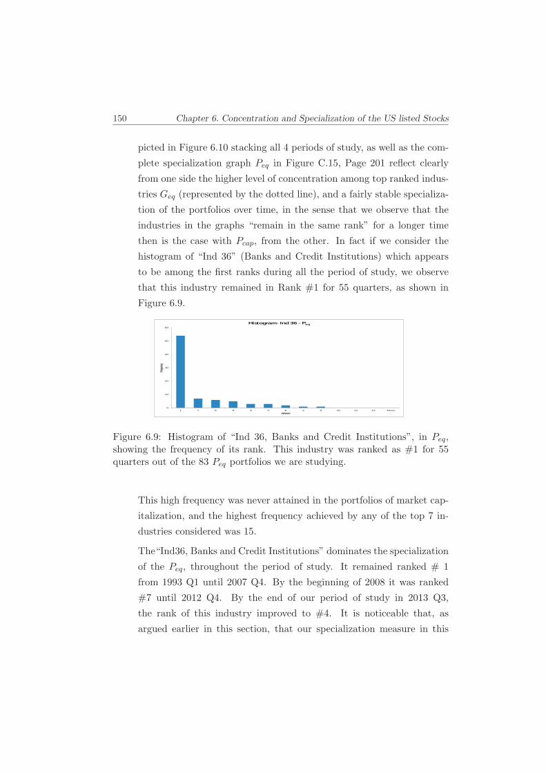
150 Chapter 6. Concentration and Specialization of the US listed Stocks
picted in Figure 6.10 stacking all 4 periods of study, as well as the com-
plete specialization graph Peq in Figure C.15, Page 201 reflect clearly
from one side the higher level of concentration among top ranked indus-
tries Geq (represented by the dotted line), and a fairly stable specializa-
tion of the portfolios over time, in the sense that we observe that the
industries in the graphs “remain in the same rank” for a longer time
then is the case with Pcap, from the other. In fact if we consider the
histogram of “Ind 36” (Banks and Credit Institutions) which appears
to be among the first ranks during all the period of study, we observe
that this industry remained in Rank #1 for 55 quarters, as shown in
Figure 6.9.
0
10
20
30
40
50
60
1 7 5 6 3 4 8 2 9 10 11 12 More
Freque
ncy
RANK
Histogram- Ind 36 - Peq
Figure 6.9: Histogram of “Ind 36, Banks and Credit Institutions”, in Peq,showing the frequency of its rank. This industry was ranked as #1 for 55quarters out of the 83 Peq portfolios we are studying.
This high frequency was never attained in the portfolios of market cap-
italization, and the highest frequency achieved by any of the top 7 in-
dustries considered was 15.
The“Ind36, Banks and Credit Institutions” dominates the specialization
of the Peq, throughout the period of study. It remained ranked # 1
from 1993 Q1 until 2007 Q4. By the beginning of 2008 it was ranked
#7 until 2012 Q4. By the end of our period of study in 2013 Q3,
the rank of this industry improved to #4. It is noticeable that, as
argued earlier in this section, that our specialization measure in this

6.2. Results: Concentration and Specialization of Peq and Pcap. 151
case is based on the number of stocks or companies included in this
industry sector, and hence our measure describes the industry of Banks
and Credit Institutions as being the industry with most listed companies
until the beginning of 2008. The interpretation of this rank variation
and its correlation with financial and economic events remains to be
researched and explained and it is beyond the scope of this work.
The Software industry, “Ind 40”, enters the top ranked industries by
1998 and reaches rank#1 for the first time in 2009 Q4 to remain later
and until 2013 Q3 among the top 5 ranked industries. The same happens
with Insurance,“Ind 38”, which starts with a solid rank#3 until 2004 Q4
where it takes the lead in the subsequent quarters and specially when
the financial crisis of the sub-primes in 2008 hits the markets where we
witness a leading rank#1 takeover from Banks and Credit Institutions,
“Ind36”. By the last quarters of our study, Insurance sector alternates
with “Ind 31, Retail”which was always raked among the top 5 industries
in Peq.
Period 1 Period 2 Period 3 Period 4
From 1993 Q1 1999 Q1 2005 Q1 2011 Q1
Till 1998 Q4 2004 Q4 2010 Q4 2013 Q3
Rank 1 Banks &CreditInstit.
Banks &CreditInstit.
Banks &CreditInstit.
Retail
Rank 2 Electric Utili-ties
IT Hardware+ Retail
Retail Software
Rank 3 Insurance Insurance not defined Insurance
Table 6.6: Peq: Summary of the specialization per industry sectors of theEqually weighted portfolios, Peq, covering the portfolios under study. TheEqually weighted portfolio exhibits a high G among the top ranked indus-tries and hence the dominance of the first 3 ranked ones define better thespecialization of these portfolios.
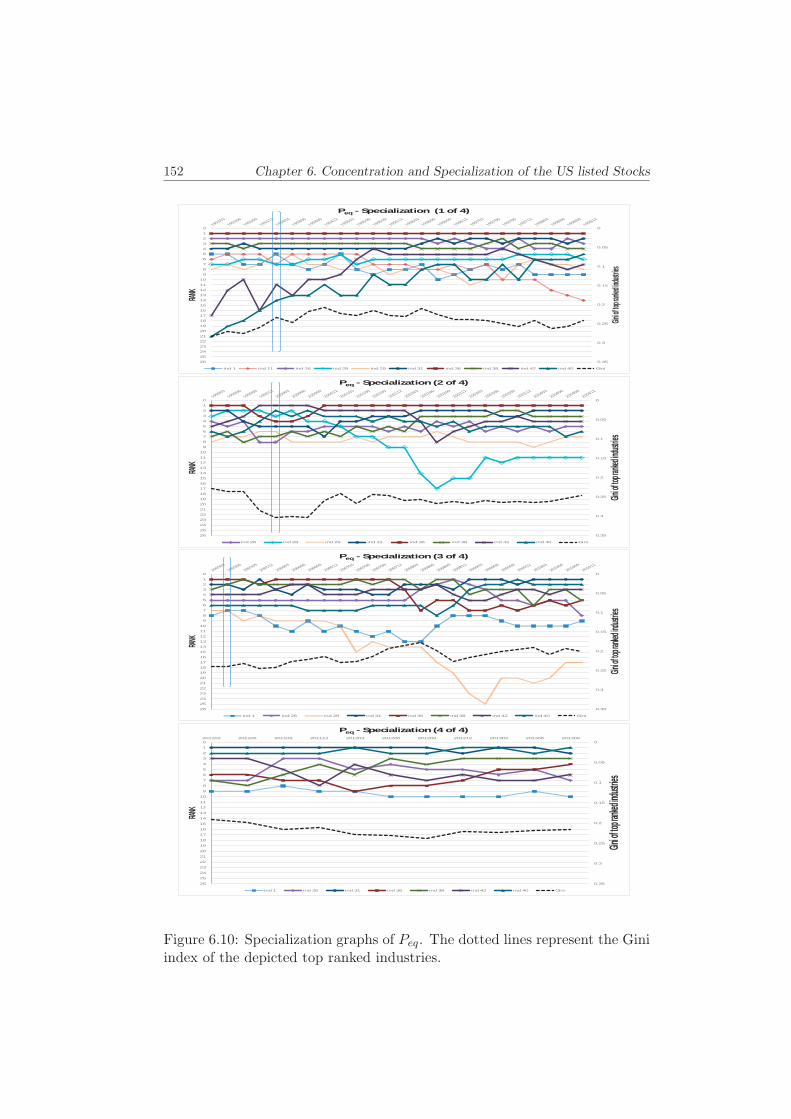
152 Chapter 6. Concentration and Specialization of the US listed Stocks
0
0.05
0.1
0.15
0.2
0.25
0.3
0.35
0
1
2
3
4
5
6
7
8
9
10
11
12
13
14
15
16
17
18
19
20
21
22
23
24
25
26
Gini of
top ran
ked ind
ustries
RANK
Peq - Specialization (1 of 4)
ind 1 ind 11 ind 26 ind 28 ind 29 ind 31 ind 36 ind 38 ind 42 ind 40 Gini
0
0.05
0.1
0.15
0.2
0.25
0.3
0.35
0
1
2
3
4
5
6
7
8
9
10
11
12
13
14
15
16
17
18
19
20
21
22
23
24
25
26
Gini of
top ran
ked ind
ustries
RANK
Peq - Specialization (2 of 4)
ind 26 ind 28 ind 29 ind 31 ind 36 ind 38 ind 42 ind 40 Gini
0
0.05
0.1
0.15
0.2
0.25
0.3
0.35
0
1
2
3
4
5
6
7
8
9
10
11
12
13
14
15
16
17
18
19
20
21
22
23
24
25
26
Gini of
top ran
ked ind
ustries
RANK
Peq - Specialization (3 of 4)
ind 1 ind 26 ind 29 ind 31 ind 36 ind 38 ind 42 ind 40 Gini
0
0.05
0.1
0.15
0.2
0.25
0.3
0.35
0
1
2
3
4
5
6
7
8
9
10
11
12
13
14
15
16
17
18
19
20
21
22
23
24
25
26
201103 201106 201109 201112 201203 201206 201209 201212 201303 201306 201309
Gini of
top ran
ked ind
ustries
RANK
Peq - Specialization (4 of 4)
ind 1 ind 26 ind 31 ind 36 ind 38 ind 42 ind 40 Gini
Figure 6.10: Specialization graphs of Peq. The dotted lines represent the Giniindex of the depicted top ranked industries.

6.2. Results: Concentration and Specialization of Peq and Pcap. 153
In practice, the specialization study of p[eq] is a study of the market
industry sectors and the market stocks during the period of study. The
information conveyed by describing the investment portfolio (like we did,
applying our method to Peq and Pcap) is rich, substantial and different
from what is conveyed by using the classic market metrics of the average
return and its moments.
6.2.2 Results Part II: Concentration of the chosen 3 portfo-
lios.
As we mentioned earlier in this chapter, and in order to complement our
study of the variation of concentration and specialization of the 83 portfolios
included in our study (from 1993 Q1 to 2013 Q3 both inclusive) we chose
three particular portfolios to analyze: i) the portfolio of absolute maximum
concentration 2000 Q1, ii) the portfolio of relative minimum concentration
occurring directly after it 2005 Q2 and iii) the portfolio of absolute minimum
concentration 1994 Q3, within the time bracket of our study. Our analysis will
include both the equally weighted portfolio allocation as well as the market
capitalization allocated portfolios related to the same dates chosen.
As outlined in Section 2.2, Page 26, we are suggesting the creation of a
weight-attribute matrix to analyze the concentration and the specialization of
a portfolio as an additional information describing an investment portfolio at
large. In the case of our three chosen portfolios, the impact matrix as detailed
in Table 2.3 Page 31 will not be depicted here because it is very big6. However
the impact matrix is elaborated separately and the results are depicted in the
subsequent tables for comparison.
6In fact the impact matrix for any of these 3 portfolios with 500 stocks included and 43industry groups will be a 500× 43 matrix that is very big to fit in this thesis.

154 Chapter 6. Concentration and Specialization of the US listed Stocks
CONCENTRATIONPcap Peq
1994 Q3 2000 Q1 2005 Q2 1994 Q3 2000 Q1 2005 Q2
HHIstk,stock level
0.0054 0.098 0.0071 0.002 0.002 0.002
rHHIstk,stock level
182 101 139 500 500 500
HHIind, in-dustry level
0.0424 0.0755 0.0429 0.0433 0.0524 0.0375
rHHIind,industrylevel
23 13 23 23 19 26
SPECIALIZATIONPcap Peq
1994 Q3 2000 Q1 2005 Q2 1994 Q3 2000 Q1 2005 Q2
G toprankedIndustries
0.11 0.24 0.09 0.18 0.18 0.15
Rank 1Comm.Utilities
IT hard-ware
Banks &CreditInstits.
Banks &CreditInstits.
IT hard-ware
Banks &CreditInstits.
Rank 2Banks &CreditInstits.
Comm.Utilities
RetailElectricUtilities
Software Retail
Rank 3Agric,Food,Beverage
Software Insurance InsuranceComm.Utilities
Insurance
Rank 4Drugs,Pharma.
Banks &CreditInstits
Software RetailBanks &CreditInstits
IT Hard-ware
Rank 5 RetailDrugs,Pharma.
IT hard-ware
Chemcls.Rubber
RetailElectricUtilities
Rank 6 Insurance RetailMiscel.Finance
Comm.Utilities
Publish.Brdcst.Cinema
Software
Rank 7Electricutilities
Photopicl,Mi-cros,Offc.Mach
Integr.Oil com-panies
Publish.Brdcst.Cinema
InsuranceAgric,Food,Beverage
Table 6.7: Descriptive summary of the three chosen portfolios: Concentrationsat the individual stock and at the industry levels and the specialization.
Table 6.7 summarizes the concentration of the three portfolios at the in-
dividual stock level as well as at the industry group’s level. It also shows

6.2. Results: Concentration and Specialization of Peq and Pcap. 155
the specialization of each portfolio, listing the top 7 ranked industries per
portfolio. The most concentrated portfolio at the stock and industry levels
alike is 2000 Q1. The portfolio least concentrated at the stock and industry
levels is 1994 Q3. A particular result is shown in the relative minimum con-
centration portfolio 2005 Q2 which exhibits a relative minimum concentration
of HHI = 0.0071 while having the same concentration at the industry level
as the portfolio with absolute minimum concentration 1994 Q3, both with
HHIind = 0.042.
Gini index, derived from the Lorenz curve, indicates the same tendency
shown by the HHI above. It is interesting to note that the market cap-
italization portfolios exhibit the lowest concentration at the industry level,
graphically apparent if the Lorenz curves are drawn for each of those portfo-
lios, as shown in Figure 6.11.

156 Chapter 6. Concentration and Specialization of the US listed Stocks
0
0.1
0.2
0.3
0.4
0.5
0.6
0.7
0.8
0.9
1
1 10 19 28 37 46 55 64 73 82 91 100 109 118 127 136 145 154 163 172 181 190 199 208 217 226 235 244 253 262 271 280 289 298 307 316 325 334 343 352 361 370 379 388 397 406 415 424 433 442 451 460 469 478 487 496
Lorenz curves of the Market cap portfolios- cumulative individual stocks' weights
Cap1994Q3 Cap2000Q1 Cap2005Q2 Peq
0
0.1
0.2
0.3
0.4
0.5
0.6
0.7
0.8
0.9
1
1 2 3 4 5 6 7 8 9 10 11 12 13 14 15 16 17 18 19 20 21 22 23 24 25 26 27 28 29 30 31 32 33 34 35 36 37 38 39 40 41 42 43 44
Lorenz Curves of three portfolios- Cumulative industry weights
Eq1994Q3 Eq2000Q1 Eq2005Q2 Cap1994Q3 Cap2000Q1 Cap2005Q2
Figure 6.11: Lorenz Curves for thew three chosen portfolios, both at theindividual stock level (top graph) and the industry level (bottom graph).
The following is a comprehensive description of the portfolios at hand:
• 1994 Q3 Market capitalization allocation: This portfolio has a relatively
low concentration measure at the levels of individual stocks as well as
industry groups, with HHI = 0.0054 and HHI = 0.0424 respectively.
It consists of 500 stocks, with a budget constraint of 1, not allowing
short sale allocations. Its rHHI = 182 at the stock level, i.e. a concen-
tration ration of 182500 = 0.36. The stocks are listed in the USA capital
market, and they are grouped in 43 industrial sectors. When the stocks
are grouped according to their industrial groups, the portfolio exhibits
a concentration level of HHI = 0.0424 equivalent to a rHHI = 23 or a

6.2. Results: Concentration and Specialization of Peq and Pcap. 157
concentration ratio of 2343 = 0.53 at the industry groups level, which is a
relatively high concentration. This portfolio is specialized in Communi-
cations utilities, Banks and Credit institutions, Agriculture, Food and
Beverages, Drugs and Pharmaceutics, Retail and Insurance. The Gini
index of the top ranked industries is low, indicating an equal special-
ization among all the top ranked industries. Its heaviest stock weighs
0.0232 (2.32%) and it belongs to the industry of communication utilities.
• 2000 Q1 Market capitalization allocation: This portfolio has a relatively
high concentration measure at the levels of individual stocks as well as
industry groups, with HHI = 0.0098 and HHI = 0.0755 respectively.
It consists of 500 stocks, with a budget constraint of 1, not allowing
short sale allocations. Its rHHI = 101 at the stock level, i.e. a concen-
tration ration of 101500 = 0.20. The stocks are listed in the USA capital
market, and they are grouped in 43 industrial sectors. When the stocks
are grouped according to their industrial groups, the portfolio exhibits
a concentration level of HHI = 0.0755 equivalent to a rHHI = 13 or
a concentration ratio of 1343 = 0.30 at the industry groups level, which
is a relatively very high concentration. This portfolio is specialized in
IT Hardware, Communications utilities, Software, Banks and Credit in-
stitutions, Drugs and Pharmaceutics, Retail and Photoopptical Micros
and office Machinery. The Gini index of the top ranked industries is
high, indicating more specialization among all the first top ranked in-
dustries. Its heaviest stock weighs 0.0387 (3.87%) and it belongs to the
industry of Software.
• 2005 Q2 Market capitalization allocation: This portfolio has a rela-
tively medium high concentration measure at the levels of individual
stocks and a low concentration at the level of industry groups, with
HHI = 0.0071 and HHI = 0.0429 respectively. It consists of 500
stocks, with a budget constraint of 1, not allowing short sale alloca-
tions. Its rHHI = 139 at the stock level, i.e. a concentration ration
of 139500 = 0.28. The stocks are listed in the USA capital market, and

158 Chapter 6. Concentration and Specialization of the US listed Stocks
they are grouped in 43 industrial sectors. When the stocks are grouped
according to their industrial groups, the portfolio exhibits a low con-
centration level of HHI = 0.0429 equivalent to a rHHI = 23 or a
concentration ratio of 2343 = 0.53 at the industry groups level, which is a
relatively a low concentration. This portfolio is specialized in Banks and
Credit institutions, Retail, Insurance, Software, IT Hardware, Miscella-
neous Finance and Integrated Oil Companies. The Gini index of the top
ranked industries is very low at Gtop = 0.09, indicating equal special-
ization among all the top ranked industries. Its heaviest stock weighs
0.0309 (3.09%) and it belongs to the industry of Financial Investments.
6.3 concluding remarks
This chapter is an example of the application of the methodology of describing
an investment portfolio that we are proposing. The descriptors are concen-
tration measures, which are estimation risk free because they are not based
on any forecasting assumption. The description we propose can be applied
to a period of time, where a certain back analysis is required or when the
analyst and the investors alike require an ext post description of the market
dynamic rather then the market performance. The methodology also can be
applied to an individual portfolio, where an ex ante description is required
free of any estimation risk. The methodology does not give any forecast on
the available moments of the asset, according to its historical data, but rather
is an instantaneous snapshot on the nature of the portfolio with respect to
its individual stocks and the attribute related to the stocks, according to the
investors’ choice. In our example this attribute of choice was the industry
group.
The approach we are proposing shows clearly the trends over a past period
of time of the market players, the industries relative weights in the portfolios,
but also the trends in specialization or , similarly, de-specialization. The
graphs we exposed in this chapter showed clearly the entry of new sectors
at the detriment of the exit of others, like Communication entering and food

6.3. concluding remarks 159
and beverages exiting, as an example.
The approach we are proposing can be the basis of an investment moni-
toring approach, tracking the changes in the concentrations of the portfolios
at hand and the tendencies of specialization along the time axis. The moni-
toring according to the concentration and specialization of the portfolios will
add valuable information to the investors’ community and will enhance the
forecasting capabilities of the investors and managers alike.

Chapter 7
Conclusion
The study set out to explore the concept of concentration and specialization
in investment portfolios and has identified the nature and form of concentra-
tion measures applied in economics and welfare studies, their application in
investment portfolios, the quality of information they would provide to the
investor and the characteristics and limitations of such measures in describing
an investment portfolio. The study has also sought to know whether the new
suggested measures of concentration and specialization introduce any estima-
tion risk into the description. The conclusion is that the suggested measures
are free of estimation risk because they do not rely on any forecasting statis-
tical calculation but are rather a direct representation of the data parameters
at hand.
General theoretical literature on the subject of measuring concentration
and specialization in investment portfolios is rare and somehow nonexistent,
since the suggested measures are usually applied in the domain of poverty,
welfare and wealth distribution. However, the literature reviewed reflected the
existence of a multitude of measures, each with a different set of characteristics
suited for some particular application in social and political economics.
The application of concentration measures to investment portfolios, as pre-
sented in our research, is a new approach to describing an investment portfolio
and this innovation should see its application with investors and investment
161
162 Chapter 7. Conclusion
managers alike. Indeed, two different portfolios can have the same statisti-
cal measures and yet differ substantially in concentration and specialization.
The techniques and measures suggested in this study are an additional tool
for monitoring and managing an investment portfolio.
The study explores the investment portfolio selection process and sheds
some light on two particular aspects of the resulting investment universe,
namely i) the concentration of the portfolio, i.e. how is the wealth distributed
among the individual stocks chosen, and ii) the specialization of the portfo-
lio, i.e. what are the attributes related to the chosen stocks that are more
prominently present than others. Indeed, in seeking to maximize his profit
and the liquidity of his portfolio, the investor places his “bet” on some partic-
ular stocks among some others based on his view of the future performance
of the portfolio. This future view requires the investor to tap into available
information related to his investment and which will help him allocate to his
wealth. The final portfolio can therefore be described ex-ante and ex-post
using historical results and observed performance, respectively. The set of
descriptors used by the investor are prone to an estimation error since they
are related to a historical data-based forecast. The study proposes to include
the descriptors of concentration and specialization as additional information
to assist the investor in his initial choice of the portfolio and also to mon-
itor the performance of his investment. The descriptors we introduce are
free of estimation risk since they are a direct measure and not a statistical
approximation of a data time series.
The study sought to answer some particular questions related to the de-
scriptors free of estimation error that it is proposing:
1. What additional information is provided by determining the concentra-
tion and the specialization of an investment portfolio?
2. What is or are the most adequate measures of concentration that best
meet the requirement of the additional information proposed?
3. Once the adequate measures are chosen, how are the concentration and
the specialization of an investment portfolio measured and how will

163
theses measures describe a constrained portfolio?
4. What added value do these proposed measures present to an investor?
The theoretical implications of the relationship between a concentrated
portfolio and its diversification potential remain an open question to be re-
searched further. It is not necessarily true that a less concentrated port-
folio is diversified, and inversely, a diversified portfolio is necessarily a less
concentrated one. The research does not reach a conclusive verdict on the
diversification and the specialization of the portfolio.
The thesis therefore concludes with a theoretical position on the neutrality
of the investment portfolio at large. The concluding conjecture states that,
apart from special cases1, no portfolio is neutral, even the equally weighted
portfolio, because there is at least one attribute that is concentrated with
respect to the others. Hence, every portfolio has a bet or a “pretension” mea-
sured by its pretension level and its specialization, and hence every portfolio
has a bias, especially the indexes, as is shown in the research.
It is also conjectured that no portfolio is diversified enough. In fact, no
portfolio can be diversified in all possible attributes of its individual stocks.
The dynamic allocation of wealth in an investment portfolio is based quite
often on the modern theory of portfolios, led by the seminal work of Markowitz
(Markowitz, 1952). The most recent development in this field lies in the the-
ory of risk weighting or allocation with respect to the risk of the asset, which is
prone to estimation error. The research is suggesting a sustainable framework
in relation with wealth allocation relying on a scalar free of estimation error:
the concentration of the portfolio. It is in this direction that the research
defines the pretension level of an investor, which gives clear and unambiguous
information on the nature and constitution of his invested portfolio. Indeed,
the pretension level being derived from the Hirschman-Herfindahl concentra-
tion measure reflects the amount of wealth allocated to each asset (or stock)
1In general, it is assumed that the number of attributes m is greater than the number ofstocks n i.e. m > n, because it is logical to think that the number of stocks is limited andthe number of attributes can be very big. However, in constrained portfolios, the numberof attributes mc can be reduced and hence mc < nc. In this case, a constrained portfoliomight be less biased than an unconstrained one.

164 Chapter 7. Conclusion
and hence reflects, in a sense, the view of the investor about the market:
where he puts his “bets” and how he distributes his wealth gives clear in-
formation on his expectation of performance and hence his pretension to the
future results of his portfolio.
The findings of the study do not challenge pre-existing views and de-
scriptors of a portfolio in general. It contributes to adding a new error-free
descriptor that will increase and improve the level and quality of the initial
information that the investors normally seeks in order to compose his port-
folio. hence the proposed method in the study contributes positively to the
decision making process during the phases of the investment, i.e. before the
portfolio is composed and later, during the life of the portfolio to monitor and
re-allocate dynamically the wealth invested. It is left to future researchers to
ascertain or refute the causal correlation between the descriptor we suggest
in our study and the performance of the portfolio.
Our research utilizes a measure of concentration and specialization that
provides a description of an investment irrespective of past values. The actual
measures used in the financial mainstream are distribution measures providing
averages and higher moments of the historical data. Our measures reflect the
changes in the investment portfolio over time, with respect to other attributes
then the periodical performance. We can express every single investment and
also every single portfolio in terms of its attributes. Our research shows
how portfolio can change over time in terms of its individual attributes and
this can be done for all the possible attributes that the investor decides to
consider. So in fact we are providing the investor an additional information
that can be of an interest to him, other then the historical changes of price
over time and its statistical derivations. Additionally, the investor usually
wants to change the composition of his portfolio by adding some new shares
or stocks and removing some others, and hence the investor not only changes
the fundamental statistics of his portfolio, but also he alters the concentration
and the specialization of his portfolio: by adding and removing some stocks
he also adds and removes those stock’s attributes. Our method measures this
effect and provides the investor with a valuable information: what is the new

165
measure of concentration and specialization of the new re-allocated portfolio.
This information is very valuable to the investor and gives an additional
insight on his investment. Our research provides a quantified measure of his
allocation strategy. By defining his “pretension” our descriptors quantify the
status of his portfolio in terms of its concentration and specialization.
The practical or empirical implications of our proposed approach is better
observed when it is applied to an index, which was simulated in the research
by applying it to several portfolio composed of the top 500 stocks listed in
the United States. Many investors who follow the indexes may have ignored
many other stocks with interesting properties and attributes that the indexes
do not include. The research shows the concentration and the specialization
of such possible indexes and the changes over time in terms of the new pro-
posed descriptors rather then in terms of the average of the price and its
volatility. The new information provided by measuring the concentration and
the specialization of the portfolio adds vital insight to the investors along
with the usual return-risk and other statistical measures. The investor knows
what additional attributes are included and excluded from the index he is
following and this additional information will modulate his decision making
process and probably his dynamic management techniques and approach: the
investor will also think in terms of the new attributes (industry sector, geo-
graphical location, ownership structures etc.) included or excluded from his
investment as a result of his allocation decisions. In fact the research shows
that many attributes were not included in the index due to the market capi-
talization allocation strategy and hence it shows a pronounced specialization
in few industrial sectors at the detriments of others.
There has been various empirical methods showing results that beat the
market index by several basis points, all based on “alternative” allocation
strategies. The research does suggests the utilization and application of the
measures of concentration and specialization as an additional information to
the investor: Not only he needs to know what is the historical performance
of such or such stocks but also what are their attributes and how do these
individual attributes influence and alter the overall concentration and spe-

166 Chapter 7. Conclusion
cialization of the portfolio at hand.
The research suggests that the stocks’ attributes like the industry sector,
the geographical location, the ownership structure or the number of employees
and their respective concentration measures do have a meaning to the investor
in addition to the statistics derived from the historical stocks’ quotes.
The popular proverb “Learn from the past but live in the present” can be
existential and somewhat reflects a philosophical perception of Time. How-
ever, it shines with a new light on the approach to investment that this re-
search is suggesting. Past quotes are useful to give the investor an idea on
their volatility but this statistical approximation has its drawbacks: it is prone
to estimation error. Concentration and specialization measures are “present
time” measures and do not rely on historical data and therefore are free of es-
timation error. It is for the wise to combine both past and present dimensions
of information in the investment decision making process.

Appendix A
Toolbox formulas and
assumptions
A.1 The Gini Index and its Decomposition
In the article “Decomposition and Interpretation of Gini and the Generalized
Entropy inequality Measures”, (Dagum, 1997a) Camilo Dagum decomposes
the Gini index and compares it to Theil, Hirschman-Herfindahl and Bour-
guignon indexes. Dagum’s aim was to introduce a three components decom-
position method with Gw (Gini index within the group), Gb ( also Gnb, the
net contribution to the Gini index between the groups) and Gt (the between
group distance or transvariation).
Given a population Q, with n units with attributes wi with i = 1, . . . , n
and a probability density f(w), a cumulative function F (w), and mean μ.
Assume the population Q is subdivided into k groups or sub-populations,
resulting in Qj , fj(w), Fj(w) and mean μj with j = 1, . . . , k. Assume also
that that each sub-population Qj ( or subgroup) has a size nj , j = 1, 2, 3 . . . , k
with∑k
j=1 nj = n. Therefore, the vector of attributes of the partitioned initial
universe Q can be expressed as:
(w1, wj , . . . , wk) = ((w11, . . . , w1n1), . . . , (w1j , . . . , wjnj), (w1k, . . . , wknk))(A.1)
Where the subindex (nk) denotes the elements of subgroup k. We also define:
167

168 Appendix A. Toolbox formulas and assumptions
pj =nj
n, and qj =
njμj
nμ, j = 1, . . . , k (A.2)
Where pj is the jth group’s population share and qj is the j
th group attribute
share1.
Gini Coefficient.
Gini (1914) defined the Gini index for a population of n units as follows:
G =Δ
2μ=
1
2n2μ
n∑i=1
n∑r=1
|wi − wr| (A.3)
Where Δ is the total Gini mean difference,i.e.:
Δ = E|wi − wr| = 1
n2
n∑i=1
n∑r=1
|wi − wr| (A.4)
If, however, we consider the populationQ as subdivided into k sub-populations,
then Equation A.3 can be written as:
G =1
2n2μ
k∑j=1
k∑h=1
nj∑i=1
nh∑r=1
|wji − whr| (A.5)
Gini within a subpopulation j.
Consider the sub-populations of Q, as per Equation A.1 above, and let Qj , j =
1, . . . , k be one subpopulation of Q. Then we define the Gini index Gjj within
the sub-population j as:
Gjj =Δjj
2μj=
1
2n2jjμj
nj∑i=1
nj∑r=1
|wji − wjr| (A.6)
Gini between two subpopulations.
Consider two sub-populations of Q, Qj and Qh with j, h = 1, . . . , k, then
we define the Gini index between the j-th and h-th sub-population (Dagum,
1987) as:
Gjh =Δjh
(μj + μh)=
1
njnh(μj + μh)
nj∑i=1
nh∑r=1
|wji − whr| (A.7)
1Please note that∑
pj =∑
qj = 1 and that∑k
j=1
∑kr=1 pjqr = 1.

A.1. The Gini Index and its Decomposition 169
Relative and Gross economic affluence.
In the same paper, Dagum (1987) introduces the definition of gross economic
affluence djh between two sub-populations as well as the directional economic
distance ration or relative economic affluence Djh between two sub-populations
as follows:
djh = Δjh − pjh, (A.8a)
Djh =(djh − pjh)
Δjh= 1− 2pjh
Δjh(A.8b)
Gini index decomposition by Dagum.
In this paragraph we refer to Dagum (1987), Theorem 3 (P.524), stating that
the total Gini index of a population of size n partitioned in k sub-populations,
as per A.1 can be decomposed into three components, as follows:
G = Gw +Gnb +Gt, (A.9a)
Ggb = Gnb +Gt (A.9b)
Where:
Gw is the weighted contribution to G of the Gini within the sub-population,
Gnb is the net contribution to G of the Gini between sub-populations,
Ggb is the gross contribution to G of the Gini between sub-populations,
Gt is the contribution to G of the transvariation between sub-populations,
and such that,

170 Appendix A. Toolbox formulas and assumptions
Gw =
k∑i=1
pjqjGjj (A.10a)
Gnb =
k∑j=2
j−1∑h=1
(pjqh + phqj)DjhGjh (A.10b)
Gt =k∑
j=2
j−1∑h=1
(pjqh + phqj)(1−Djh)Gjh (A.10c)
Ggb =k∑
j=2
j−1∑h=1
(pjqh + phqj)Gjh = Gnb +Gt (A.10d)
Gini decomposition: Particular cases to note.
The following two cases that we note hereafter are proven in Dagum (1987)
paper, P.526, under Corollary 3, and Corollary 5 respectively.
Case 1: μj = μ. In the assumption of equal means between the entire
group μ and the sub-populations μj then qj =nj
n = pj , with j = 1, 2, . . . , k.
The corollary 3 (Dagum, 1987) proves that, iff μj = μ, Djh = 0 and
Gw =
k∑j=1
p2jGjj (A.11a)
Gt = 2
k∑j=2
j−1∑h=1
pjphGjh (A.11b)
Gnb = 0 (A.11c)
Case 2: k sub-populations do not overlap. In the assumption that
the measured attribute density functions (in our case the weights of the stocks)
of the k populations do not overlap, (Dagum, 1987) Corollary shows that
pjh = 0 and djh = Δjh leading to Djh = 1 and
G = Gw +Gnb , since : Gt = 0 and Gnb = Ggb (A.12)

A.1. The Gini Index and its Decomposition 171
Case 3: Initial Universe is equally weighted. This is an assumption
which is particular to investment portfolio rather then to population income
or social welfare. In the case the initial universe, in our case the portfolio, is
equally weighted, i.e. wi =1n for all i = 1, 2, 3, . . . , n then, intuitively and by
definition G = 0, reflecting a total equality within the portfolio.
If we divide the portfolio into subgroups, according to certain attributes
of choice, then for any subpopulation Qj with j = 1, 2, 3, . . . , k where k is the
number of subgroups, then wj1 = wj2 = · · · = wjnj =1n , and consequently
Δjj = 0 (Equation A.4) and Gjj = 0 (Equation A.6) as well as Gjh = 0
(Equation A.7). Consequently, the decomposed Gini index becomes:
G = Gw = Gnb = Gt = Ggb = 0 (Equation A.9a).
The particularity of the equally weighted portfolio vis-a-vis its special-
ization resides in the fact that, although the decomposed G index indicates
no specialization, the portfolio might eventually be specialized when the at-
tributes are taken into consideration. Suppose that our hypothetical portfolio
of 10 stocks was equally weighted, with w1 = w2 = w3 = · · · = w10 =110 = 0.1.
Its G = 0 as well as all its decompositions, but, from Table 5.3 Page 114 we
can see that the portfolio is specialized in Pharmaceutical companies (four
companies out of the ten available), when the attribute “industry group” is
described.
Hence, we conclude that the method we are introducing to mea-
sure the specialization within a portfolio using Gini index and its de-
composition is not applicable when the portfolio is equally weighted.
A possible simple measure of specialization in this case would be the ratio ofnj
n where nj is the number of stocks within a subgroup (corresponding to a
particular attribute) and n is the total number of stocks in the portfolio2.
Gini index including null entries: Gnull.
The Gini index including null entries Gnull is a new measure we introduce
in this thesis to reflect the exact situation of the specialization within a sub-
2All weights being equal, this measure ofnj
nproxies the average μj of the subgroup. In
fact, μj =∑nj
i=1(wi)
n=
nj
n2

172 Appendix A. Toolbox formulas and assumptions
population. It is defined as the Gini index of the whole sub-population, in-
cluding the null entries. The Gnull is not related to the decomposed Gini
index we discuss above. It is an additional measure to further assess the spe-
cialization of a portfolio of investment.
A sub-populationQj , j = 1, . . . , k with its entries as follows: (wj1, wj2, . . . , wjnj )
which was referred to throughout our thesis, assumes no null entries within
the sub-population, since , in the measurement of income concentration where
all these formulas are applied, there is no coherent meaning to a null entry
because it reflects an individual with no income whatsoever. Hence, all the
members of the sub-population Qj are not null, i.e. they represent an in-
come to a certain given individual in the chosen sub-population. However, in
our application of the Gini index to measure specialization in a portfolio, the
sub-populations (or subgroups) chosen to reflect the attributes we want to
describe include null entries. This is understandable given the fact that, if we
are focusing on the geographic locations of the stocks as our chosen attribute,
we understand that some of the stocks belong to a certain location whereas
the others do not i.e. we assume a priori, that within a given portfolio and
with a given attribute under study, no single stock can belong to two differ-
ent subgroups at the same time, within the same attribute3. We can fairly
describe our ten-stock portfolio, vis-a-vis the geographic location as:
Subgroup 1: Six stocks belonging to Japan and four stocks not belonging to
Japan, and,
Subgroup 2: Four stocks belonging to the USA and six stocks not belonging
to the USA.
We are proposing to introduce a new Gini index that includes the null entries
to reflect the relative specialization of one subgroup with respect to the other.
Consider, for example, the attribute “industry group” reflected in Table
5.7, which shows 1 stock in each of Mining and Retail subgroups. If we
apply the A.3 above to the above subgroups, with 1 stock only present in
3This is to say, if we choose the geographic location as an attribute under study, no singlestock can belong to two different locations at the same time. Hence, given the ten stocksthat are included in our hypothetical portfolio we observe that six out of the ten stocks arefrom Japan and the other four out of ten are from US

A.2. The HHI or Hirschman-Herfindahl Index 173
each subgroup, we will have a Gjj = 0 (please refer to Table 5.7, Page 119,
row 2b) showing total equality and lack of specialization: all the wealth is
equally allocated among all the units of the subgroup. However, from an
investment perspective, it is clear that the opposite is true: this subgroup
exhibits a high specialization since all the wealth allocated to this subgroup
is concentrated in 1 stock among all the 10. Therefore, in order to describe
better this particularity in investment portfolio, we introduce theGjnull, which
is the Gini index of a subgroup j, taking into consideration the null entries4
as follows:
Gjnull=
1
2n2μjnull
n∑i=1
n∑r=1
|wi − wr| (A.13)
Where μjnullis the mean of subgroup j taking into consideration the null
entries, and n is the total number of stocks in the portfolio. In our example
of industry group, this is reflected in Table 5.7, Page 119, row 2a. The value of
Gjnullcorresponding to the “All Groups” category represents the Gini index
between the total weights of each subgroup.
A high Gjnullindicates the presence of a specialization within the subgroup
because it indicates that the weights of the stocks within the subgroup are not
equally distributed. A low Gjnull(between 0 and 0.25) indicates the absence
of specialization within the group (i.e. no subgroup’s weight is high compared
to the other subgroups).
A.2 The HHI or Hirschman-Herfindahl Index
HHI Index.
We define the HHI as the sum of the squares of the weights, i.e.
HHI =∑i
( xi∑n1 xi
)2=
∑w2i . (A.14)
4This concept of null entries in concentration measure is very relevant in elections anal-ysis, where those who did not vote for a particular candidate must be taken into account inthe analytical conclusions as discussed by Taagapera (1979).

174 Appendix A. Toolbox formulas and assumptions
In our tables, when the HHI used reflects the “All Groups” concentration,
as well as the per subgroup concentration. The values of the subgroups con-
centration do not add to the HHI of all groups.
cHHI: Corrected HHI
The HHI has an upper bound of 1 when total concentration is achieved and
a lower bound of 1n when minimum concentration is achieved in an equally
weighted portfolio. It is however possible to bound the HHI from 0 to 1
instead of 1/n to 1 resulting in a Corrected HHI:
Corrected HHI = cHHI = 1− 1−HHI
1− 1n
(A.15)
The cHHI will have a value of zero (instead of 1n) when minimum concentra-
tion is achieved and will remain with 1 as its upper bound when maximum
concentration is reached.
rHHI: Reverse HHI index.
rHHI =1
HHI(A.16a)
rHHI
n=
1
n×HHI(A.16b)
The reverse HHI is a concentration measure that indicates the number
of equally weighted stocks in a portfolio that would generate the same HHI.
This gives an indication of the “degree” of concentration of a given portfolio
vis-a-vis the number of stocks included. As an illustration, if a portfolio of 10
stocks has an HHI = 0.5 it can be said that this portfolio is equivalent to a
rHHI = 10.5 = 2 equally weighted stocks’ portfolio.
If the portfolio of n stocks is equally weighted then its HHI = 1n and its
rHHI = n which is the maximum value that rHHI can take, i.e.
1 ≤ rHHI ≤ n

A.2. The HHI or Hirschman-Herfindahl Index 175
It is useful to be able to compare rHHI of various portfolios or subgroups
within a portfolio to assess the amount or the level of concentration in terms
of the total number of stocks n. We suggest a per unit measure of equally
weighted equivalent number of stocks by dividing the rHHI by n , rHHIn , a
measure that appears in row 11 of our Tables ??, ??, ??, ?? and 5.7.


Appendix B
Portfolio Pretension Level
B.1 The HHI and the Portfolio Pretension Level
If an investor chooses to invest equal wealth in each stock, i.e. w1 = w2 =
w3 · · · = wn = 1/n, then it can be assumed that he does not have any prefer-
ence of one stock or sector over the other, and we define this investor attitude
as a minimum pretension level of investment. The more the allocation de-
viates from the 1/n allocation strategy, the more wealth is invested in one
stock against the others within the n stocks chosen. This indicates a higher
pretension level, in the sense that the investor assumes or pretends that the
latter choice, different from the lowest possible level of pretension, will even-
tually outperform the 1/n portfolio. Although more weight is invested in
some stocks and less in others,and hence creating a portfolio with a higher
pretension level, the choice remains a pretension or ex-ante prognostic. Ex-
post results could be different from the investor’s “pretension” and therefore
a higher pretension level is definitely not a guarantee of a higher or a better
performance.
Definition of pretension level
1. We define a pretentious portfolio as one with a weight matrix [wi], re-
177
178 Appendix B. Portfolio Pretension Level
sulting in a concentration index HHI, such that :
HHI ≥ 1
n
i.e. the more the portfolio allocation deviates from the equally weighted
allocation 1/n the more pretension of the investor.
2. The minimum pretension portfolio is a unique portfolio being the 1/n
or equally weighted portfolio whose HHI = 1n .
3. A given pretension level, i.e. a given value of HHI can be generated by
various matrices [wi], hence a given pretension level does not impose
a unique portfolio, but rather an isometric HHI Portfolio Opportunity
Set: POS. We further define the Portfolio Pretension Set (PPS) as the
POS that satisfies a unique pretension level, a chosen HHI value, or the
ISO-HHI-POS.
4. From 3. above we conclude that for a given pretension level HHI, we
have a variety of resulting POS (i.e. the several sets of [wi] satisfying
HHI=h), and hence a given HHI value or level does not specify a unique
return value1. In fact, the return of a portfolio is R = [wi]T .[ri], where
[ri] = [r1, r2, r3, r4, . . . rn] is the return vector of each individual stock
included in the chosen universe. It is clear that the value of R is not
1A given pretension level, i.e. a given value of HHI can be generated by vari-ous vectors [wi], hence a given pretension level does not impose a unique portfolio butrather an ISO–HHI Portfolio Opportunity Set (POS).Intuitively, and since the HHI isnot a ranking sensitive index, for each value of HHI corresponding to a weight vector[wi] = [w1, w2, w3, . . . , wn], the same value of HHI is attained with a combination of theelements of [wi], among other possibilities. For example a weight vector of (0.3, 0.5, 0.2) hasthe same HHI = 0.38 as the vector (0.5, 0.3, 0.2) and the vector (0.2, 0.5, 0.3). Please notethat theoretically the POS set of 3 stocks satisfying a HHI = 0.38 is obtained by solvingthe quadratic equation:
w21 + w2
2 + w23 = 0.38
subject to the following constraints:
w1 + w2 + w3 = 1 (the budget constraint), and
w1, w2 and w3 > 0 (i.e no short selling allowed).

B.2. Towards a return–risk–pretension portfolio description 179
unique for a given HHI, since the given HHI does not define a unique
weight vector [wi].
It is practical to normalize the measure of pretension and define a pre-
tension level of 0 as a no–pretension portfolio hence relative to an equally
weighted portfolio and define a pretension level of 1 as a maximum preten-
sion level resulting from a totally concentrated portfolio in one single stock.
Hence the pretension level or pretension index PRET is bounded as follows:
0 ≤ PRET ≤ 1 , assuming no short selling.
This requires the correction of the lower bound of HHI from 1n to 0. We
define the pretension index or pretension level of a portfolio PRET = cHHI
as being equal to the corrected HHI as follows:
PRET = cHHI = 1− 1−HHI
1− 1n
(B.1)
Where a minimum pretension portfolio, or a non-pretentious portfolio, is rep-
resented by a cHHI = 0 in fact corresponding to a minimum HHI = 1/n.
B.2 Towards a return–risk–pretension portfolio de-
scription
As discussed earlier, the process of deciding on an investment portfolio is a
matter of subjective choices based on some defined criteria that depend on the
investor. If the investor has no preference or pretension of any one stock over
the others he will eventually chose an equally weighted portfolio. If however
he has valuable information or market data or wants to take more risk he will
move from the equally weighted portfolio to a portfolio where more weight
is put on some particular stocks at the detriment of the others, assuming
no short sales. In this case, the concentration level is measured in terms of
budget fractions invested per one stock or equivalently by its weight fraction
contribution within the portfolio [wi] .
The concentration level or pretension level of a portfolio is a totally objective

180 Appendix B. Portfolio Pretension Level
measure not depending on any estimation error or approximation of distri-
bution. In fact it is a measure independent from risk and return. It reflects
objectively the subjective choice of the investor. The more the investor likes
risk or the more information he believes he has or perceives from the mar-
ket, the more concentrated the final chosen portfolio is. It is not possible to
separate the investor’s perception and preference effect from of the resulting
portfolio’s concentration. This relationship between concentration resulting
from the investor’s choices and preferences was defined earlier as pretension.
In its broad sense, the pretension level describes, in an estimation free sense
,the resulting preferences and perceptions of the investor. It is an additional
descriptor of the investment portfolio, error free and estimation free. Each
and every portfolio is earmarked with a pretension level that is the same
ex–post and ex–ante if the weights are not reallocated.
Figure B.1: Relationship between the cHHI or pretension level (horizontalaxis) and Total return and Standard deviation of a hypothetical portfolio of3 stocks, using a generated POS of around 10,000 portfolios.
In Figure B.1 we used 3 stocks to generate 10,000 different possible port-
folios or POS, hence generating 10,000 matrices [w1, w2, w3] including the 4
particular portfolios: (i) the equally weighted portfolio [1/3, 1/3, 1/3] and (ii)
the three one-stock portfolios, [1, 0, 0], [0, 1, 0], [0, 0, 1]. From the graphs in
Figure B.1 we can observe the following:

B.2. Towards a return–risk–pretension portfolio description 181
a) The 4 particular portfolios mentioned above appear very clearly in the
graphs. At the 0 pretension level, tangent to the y–axis, we find the
the equally weighted portfolio At the pretension level of 1 we find the 3
one-stock portfolios.
b) The portfolio of maximum return (upper right leg of return graph) is
the portfolio consisting of the stock having the highest return among
the three used at a pretension level of 1, with three different portfolios.
c) The equally weighted portfolio is not necessarily the highest return port-
folio or the lowest risk possible portfolio.
d) The portfolio of minimum Standard Deviation = 0.0211 (minimum risk)
occurs at a pretension level of cHHI= 0.4087 with [wi] = [0.27, 0.73, 0]
and a return of .0058; this point is graphically identified as the tangent
to the standard deviation graph and parallel to the x–axis.
e) The particularity of the minimum variance portfolio mentioned in d)
above is that it does not include stock s3. This is graphically clear since
the tangent line to the standard deviation graph lies to the right of the
vertex of the parabola joining stocks s1 and s2. In fact, the extremums of
the parabolas joining each 2 stocks pairwise occur at the value cHHI=
1/4. In general, for any portfolio of n stocks the pretension level of
any sub–portfolio of 2 of its stocks, equally weighted, is represented
by the general weight matrix [wi] = [0, 0, . . . , 0.5, . . . , 0.5, . . . ] to which
corresponds the value of HHI = 12 , and a cHHI2 of:
cHHI2 = 1− 1− 12
1− 1n
= 1− 1
2(1− 1n)
= 1− n
2(n− 1)(B.2)
With n = 3 then cHHI2 =14 .
When n → ∞ then cHHI2 = 1− 1
2(1− 1n)
→ 12 .
f) Building on the results of e) above and using the same derived relation-
ship, cHHI2, we can conclude that the (cHHI2 − ε) point is the max-
imum value of cHHI that a portfolio can reach, i.e. cHHI < cHHI2,

182 Appendix B. Portfolio Pretension Level
if the investor wants to include each and every available stock in his
portfolio. Hence, when n is big enough a pretension level cHHI < 0.5
will ensure that all available stocks are included in the portfolio.
g) We observe that the minimum standard deviation value, σmin = 0.0211
occurs at a point lower than the lowest standard deviation of one single
stock (in our example it is 0.0224). This clearly reflects the effect of
correlation among the 3 stocks. Indeed the effect of the correlation
on the cHHI vs Standard deviation curve is to tilt it slightly counter
clockwise, allowing for a lower point the lowest possible single stock
standard deviation value.
h) For example, let us fix a pretension value at 0.2. As discussed earlier,
this pretension value is generated by an infinitely many possible vectors
of weights. However, there is only one vector which will have this pre-
tension level and yield the maximum possible return. This can be found
by solving the following set of equations:
w21 + w2
2 + w23 = 0.2
s.t. w1 + w2 + w3 = 1 (budget constraint)
max Rp = [w1r1 + w2r2 + w3r3]
Solving this set of equations will result in the following weight vec-
tor: [w0.2] = [0.63, 0.21, 0.16]0.2 with a corresponding Rmax0.2 ,= 0.0072
and a σ0.2 = 0.025, which is clearly greater then σmin = 0.0211. This
shows that the graphs of cHHI vs. Return,(RET), and Standard devi-
ation,(STDDEV), are consistent with the efficient frontier theory.
i) The fact that the same return level can be achieved by more then one
weight vector, implies that the pretension level can be used to monitor
the changes in a portfolio’s weights across time. This means that if
the investor dynamically reallocates (reallocation = change of weight =

B.2. Towards a return–risk–pretension portfolio description 183
change in pretension level) the weights to adjust for a desired return or
desired risk level, then the pretension level would depict this change.
This is similar to drawing a horizontal line on Figure B.1 above, hence
fixing a level for return and σdesired. This in turn yields, at least graphi-
cally, the bracket of pretension level and hence concentration level where
the portfolio reallocation will lead.

Appendix C
Tables and Graphs Related to
Peq and Pcap.
This Appendix includes all teh graphs related to the specialization analysis
of the portfolios Peq and Pcap. The analysis corresponds to our initial choice
of Industry sector attribute, therefore the graphs appearing in this Appendix
are those related to the industry sectors.
As mentioned in Chapter 6, PART I, the analysis is related to specifying
the specialization variation of two portfolios, the equally weighted and the
market capitalization portfolio.
We have identified 44 industry sectors using the GICS1 code that were
downloaded from CRSP/COMPUSTAT. In our analysis we shall use a simple
reference system to designate the available 44 industry sectors from Ind 1
to Ind 44, as it will appear on the graphs. Table C.1 is a mapping of the
simplified coding we are using in the analysis.
1GICS, The Global Industry Classification Standard (GICS) is an industry taxonomydeveloped in 1999 by MSCI and Standard & Poor’s (S&P) for use by the global financialcommunity. In the database we downloaded from CRSP/COMPUSTAT, it is referred to asGIND and SUBGIND (Wikepedia definition).
185

186 Appendix C. Peq and Pcap Related Tables and Graphs
Simplified Industry Codes
Code Description Code Description
Ind 1 Agriculture, Food, Beverage Ind 23 Govt. Aircraft and Defense
Ind 2 Beer, Liquor and Tobacco Ind 24 Land and Water Transportation
Ind 3 Basic Minerals and Metals Ind 25 Airlines
Ind 4 Oil and Coal Resources Ind 26 Electric Utilities
Ind 5 Integrated Oil Companies Ind 27 Gas and Other Public Utilities
Ind 6 Oil Drilling and Services Ind 28 Communications Utilities
Ind 7 Oil Distribution Ind 29 Publishing, Broadcasting, Cinema
Ind 8 Construction Materials Ind 30 Restaurants, Hotels, Theaters
Ind 9 Forest Products, Paper Ind 31 Retail
Ind 10 Construction, Homebuilding Ind 32 Healthcare and Hospitals
Ind 11 Chemicals, Rubber Ind 33 Information, Services
Ind 12 Metal Products, Machinery Ind 34 Real Estate Development
Ind 13 Instruments Ind 35 Financial Investments
Ind 14 Mainframes and Minicomputers Ind 36 Banks and Credit Institutions
Ind 15 Photooptical, Micros, Offc.Mch. Ind 37 Miscellaneous Finance
Ind 16 Textiles and Apparel Ind 38 Insurance
Ind 17 Drugs and Pharmaceuticals Ind 39 Biotechnology
Ind 18 Soaps and Cosmetics Ind 40 Software
Ind 19 Furniture, Household Items Ind 41 Cellular, Wireless
Ind 20 Consumer Durables Ind 42 IT Hardware
Ind 21 Cars and Trucks Ind 43 Reits
Ind 22 Commercial Aircraft, Components Ind 44 Wholesale
Table C.1: Reference system to designate the available 44 industry sectorsreferred to in the analysis
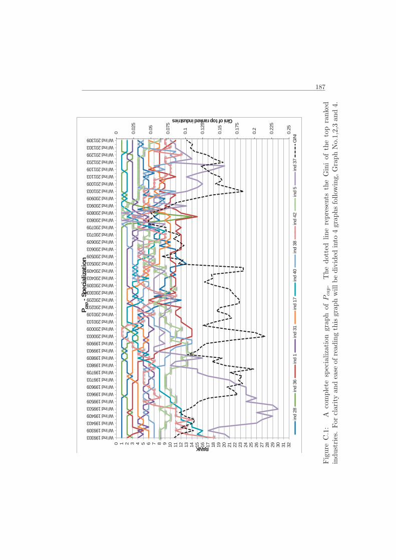
187
0 0.02
5
0.05
0.07
5
0.1
0.12
5
0.15
0.17
5
0.2
0.22
5
0.25
0 1 2 3 4 5 6 7 8 9 10 11 12 13 14 15 16 17 18 19 20 21 22 23 24 25 26 27 28 29 30 31 32
W/Ind 199303W/Ind 199309W/Ind 199403W/Ind 199409W/Ind 199503W/Ind 199509W/Ind 199603W/Ind 199609W/Ind 199703W/Ind 199709W/Ind 199803W/Ind 199809W/Ind 199903W/Ind 199909W/Ind 200003W/Ind 200009W/Ind 200103W/Ind 200109W/Ind 200203W/Ind 200209W/Ind 200303W/Ind 200309W/Ind 200403W/Ind 200409W/Ind 200503W/Ind 200509W/Ind 200603W/Ind 200609W/Ind 200703W/Ind 200709W/Ind 200803W/Ind 200809W/Ind 200903W/Ind 200909W/Ind 201003W/Ind 201009W/Ind 201103W/Ind 201109W/Ind 201203W/Ind 201209W/Ind 201303W/Ind 201309
Gini of top ranked industries
RANK
P cap
-Spe
cial
izat
ion
ind
28in
d 36
ind
1in
d 31
ind
17in
d 40
ind
38in
d 42
ind
5in
d 37
GIN
I
Figure
C.1:
Acomplete
specialization
graph
ofPca
p.
Thedotted
linerepresents
theGiniofthetop
ranked
industries.For
clarity
andease
ofreadingthisgraphwillbedivided
into
4graphsfollow
ing,GraphNo.1,2,3
and4.
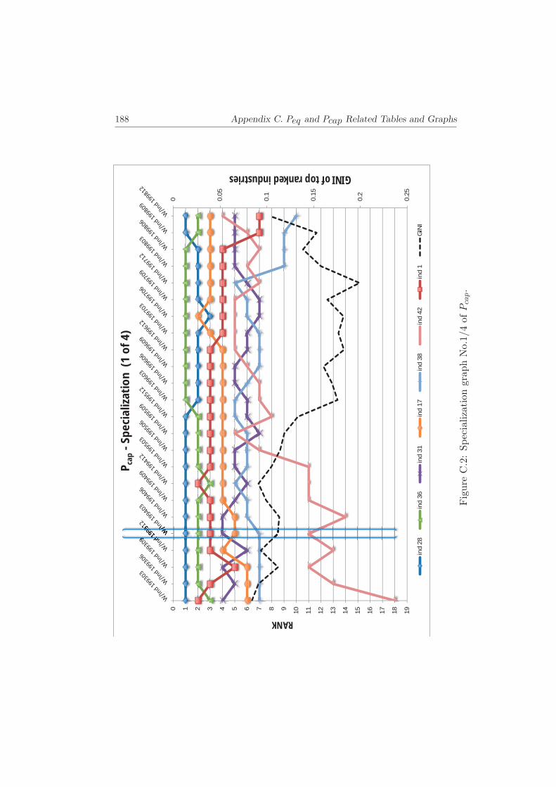
188 Appendix C. Peq and Pcap Related Tables and Graphs
0 0.05
0.1
0.15
0.2
0.25
0 1 2 3 4 5 6 7 8 9 10 11 12 13 14 15 16 17 18 19
GINI of top ranked industries
RANK
P cap
-Spe
cial
izat
ion
(1 o
f 4)
ind
28in
d 36
ind
31in
d 17
ind
38in
d 42
ind
1G
INI
Figure
C.2:SpecializationgraphNo.1/4ofPca
p.
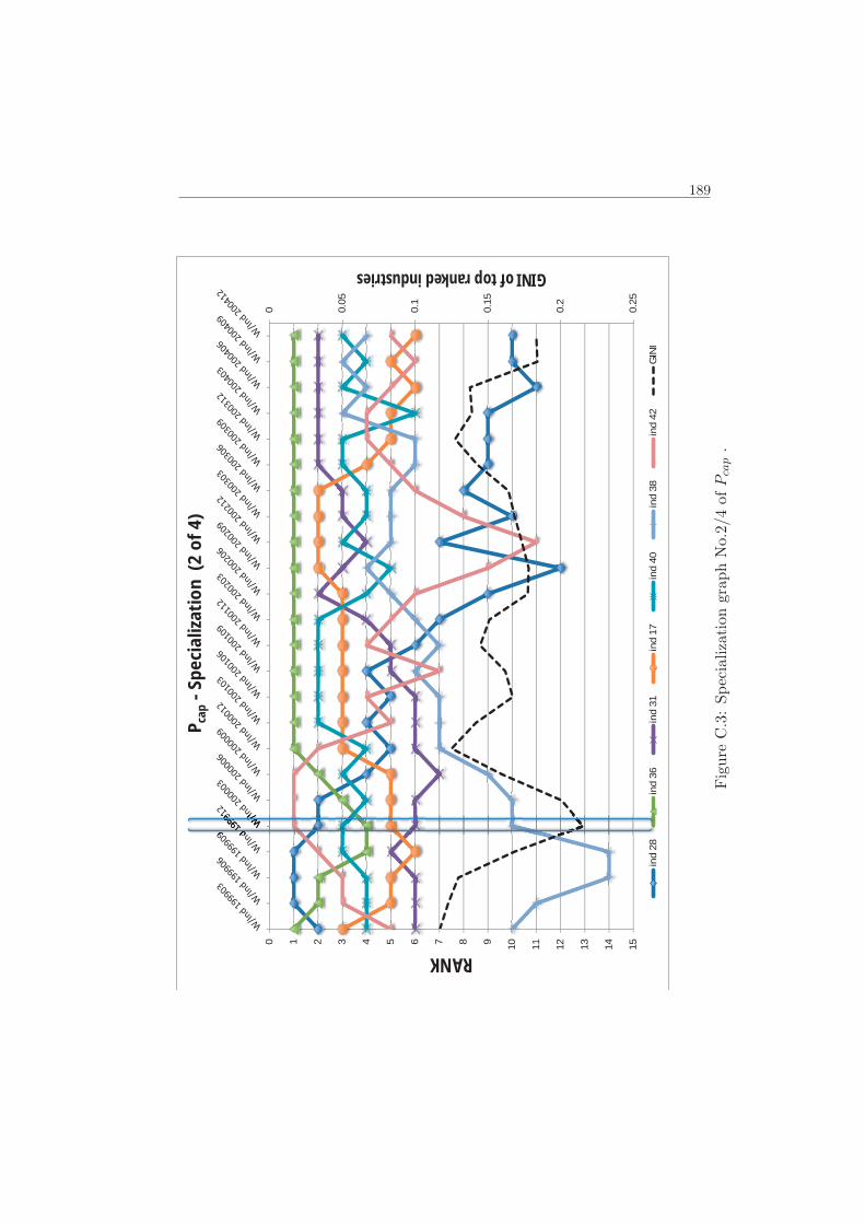
189
0 0.05
0.1
0.15
0.2
0.25
0 1 2 3 4 5 6 7 8 9 10 11 12 13 14 15
GINI of top ranked industries
RANK
P cap
-Spe
cial
izat
ion
(2 o
f 4)
ind
28in
d 36
ind
31in
d 17
ind
40in
d 38
ind
42G
INI
Figure
C.3:SpecializationgraphNo.2/4ofPca
p.

190 Appendix C. Peq and Pcap Related Tables and Graphs
0 0.02
0.04
0.06
0.08
0.1
0.12
0.14
0.16
0.18
0.2
0 1 2 3 4 5 6 7 8 9 10 11 12 13 14 15 16 17
GINI of top ranked industries
RANK
P cap
-Spe
cial
izat
ion
(3 o
f 4)
ind
36in
d 31
ind
40in
d 38
ind
42in
d 5
ind
37G
INI
Figure
C.4:SpecializationgraphNo.3/4ofPca
p.

191
0 0.02
0.04
0.06
0.08
0.1
0.12
0.14
0.16
0.18
0 1 2 3 4 5 6 7 8 9 10 11 12
W/I
nd20
1103
W/I
nd20
1106
W/I
nd20
1109
W/I
nd20
1112
W/I
nd20
1203
W/I
nd20
1206
W/I
nd20
1209
W/I
nd20
1212
W/I
nd20
1303
W/I
nd20
1306
W/I
nd20
1309
GINI of top ranked industries
RANK
P cap
-Spe
cial
izat
ion
(4 o
f 4)
ind
36in
d 31
ind
17in
d 40
ind
38in
d 5
ind
28G
INI
Figure
C.5:SpecializationgraphNo.4/4ofPca
p.

192 Appendix C. Peq and Pcap Related Tables and Graphs
Figure C.6: Histogram No.1/9 of the frequency and rank of all the industrysectors comprised in Pcap.

193
Figure C.7: Histogram No.2/9 of the frequency and rank of all the industrysectors comprised in Pcap.

194 Appendix C. Peq and Pcap Related Tables and Graphs
Figure C.8: Histogram No.3/9 of the frequency and rank of all the industrysectors comprised in Pcap.

195
Figure C.9: Histogram No.4/9 of the frequency and rank of all the industrysectors comprised in Pcap.

196 Appendix C. Peq and Pcap Related Tables and Graphs
Figure C.10: Histogram No.5/9 of the frequency and rank of all the industrysectors comprised in Pcap.

197
Figure C.11: Histogram No.6/9 of the frequency and rank of all the industrysectors comprised in Pcap.

198 Appendix C. Peq and Pcap Related Tables and Graphs
Figure C.12: Histogram No.7/9 of the frequency and rank of all the industrysectors comprised in Pcap.

199
Figure C.13: Histogram No.8/9 of the frequency and rank of all the industrysectors comprised in Pcap.

200 Appendix C. Peq and Pcap Related Tables and Graphs
Figure C.14: Histogram No.9/9 of the frequency and rank of all the industrysectors comprised in Pcap.

201
0 0.05
0.1
0.15
0.2
0.25
0.3
0.35
0 1 2 3 4 5 6 7 8 9 10 11 12 13 14 15 16 17 18 19 20 21 22 23 24 25 26
199303199309199403199409199503199509199603199609199703199709199803199809199903199909200003200009200103200109200203200209200303200309200403200409200503200509200603200609200703200709200803200809200903200909201003201009201103201109201203201209201303201309
Gini of top ranked industries
RANK
P eq
-Spe
cial
izat
ion
ind
1in
d 11
ind
12in
d 26
ind
28in
d 29
ind
31in
d 36
ind
38in
d 42
ind
40G
ini
Figure
C.15:
Acomplete
specialization
graph
ofPeq.
Thedotted
linerepresents
theGiniofthetop
ranked
industries.Forclarity
andease
ofreadingthisgraphwillbedivided
into
4graphsfollow
ing,GraphNo.1,2,3
and4.

202 Appendix C. Peq and Pcap Related Tables and Graphs
0 0.05
0.1
0.15
0.2
0.25
0.3
0.35
0 1 2 3 4 5 6 7 8 9 10 11 12 13 14 15 16 17 18 19 20 21 22 23 24 25 26
Gini of top ranked industries
RANK
P eq
-Spe
cial
izat
ion
(1 o
f 4)
ind
1in
d 11
ind
26in
d 28
ind
29in
d 31
ind
36in
d 38
ind
42in
d 40
Gin
i
Figure
C.16:SpecializationgraphNo.1/4ofPeq.

203
0 0.05
0.1
0.15
0.2
0.25
0.3
0.35
0 1 2 3 4 5 6 7 8 9 10 11 12 13 14 15 16 17 18 19 20 21 22 23 24 25 26
Gini of top ranked industries
RANK
P eq
-Spe
cial
izat
ion
(2 o
f 4)
ind
26in
d 28
ind
29in
d 31
ind
36in
d 38
ind
42in
d 40
Gin
i
Figure
C.17:SpecializationgraphNo.2/4ofPeq
.

204 Appendix C. Peq and Pcap Related Tables and Graphs
0 0.05
0.1
0.15
0.2
0.25
0.3
0.35
0 1 2 3 4 5 6 7 8 9 10 11 12 13 14 15 16 17 18 19 20 21 22 23 24 25 26
Gini of top ranked industries
RANK
P eq
-Spe
cial
izat
ion
(3 o
f 4)
ind
1in
d 26
ind
29in
d 31
ind
36in
d 38
ind
42in
d 40
Gin
i
Figure
C.18:SpecializationgraphNo.3/4ofPeq
.

205
0 0.05
0.1
0.15
0.2
0.25
0.3
0.35
0 1 2 3 4 5 6 7 8 9 10 11 12 13 14 15 16 17 18 19 20 21 22 23 24 25 262011
0320
1106
2011
0920
1112
2012
0320
1206
2012
0920
1212
2013
0320
1306
2013
09
Gini of top ranked industries
RANK
P eq
-Spe
cial
izat
ion
(4 o
f 4)
ind
1in
d 26
ind
31in
d 36
ind
38in
d 42
ind
40G
ini
Figure
C.19:SpecializationgraphNo.4/4ofPeq
.


List of Tables
2.1 Hypothetical 10 stocks portfolio resulting from a screening vector 28
2.2 Detailed Weight-attribute matrix . . . . . . . . . . . . . . . . . 30
2.3 Detailed Impact matrix . . . . . . . . . . . . . . . . . . . . . . 31
3.1 Determinants of choice for the Indexes. . . . . . . . . . . . . . . 69
3.2 Effect of big weights on HHI . . . . . . . . . . . . . . . . . . . . 72
3.3 Gini index . . . . . . . . . . . . . . . . . . . . . . . . . . . . . 78
3.4 Effect of the weight transfer on Gini . . . . . . . . . . . . . . . 79
3.5 Summary of the HHI and Gini indexes characteristics. . . . . . 82
4.1 Count of companies in the 2008 USA stock market . . . . . . . 96
5.1 Hypothetical 10 stocks portfolio, equally weighted. . . . . . . . 102
5.2 Hypothetical 10 stocks portfolio, equally weighted, with two
attributes . . . . . . . . . . . . . . . . . . . . . . . . . . . . . . 104
5.3 Hypothetical 10 stocks portfolio resulting from a screening vector114
5.4 Detailed Weight-Criteria matrix . . . . . . . . . . . . . . . . . . 116
5.5 Detailed Impact matrix . . . . . . . . . . . . . . . . . . . . . . 117
5.6 HHI and Gini indexes summary. . . . . . . . . . . . . . . . . . 119
5.7 Industry group attribute: Gini and HHI toolbox output. . . . . 119
6.1 Mapping of analysis results . . . . . . . . . . . . . . . . . . . . 130
6.2 Top and Bottom concentration values for Pcap at stocks level . 133
6.3 Top and Bottom concentration values for Pcap at Industry clus-
ters level . . . . . . . . . . . . . . . . . . . . . . . . . . . . . . . 136
207

208 List of Tables
6.4 Top and Bottom concentration values for Peq at Industry clus-
ters level . . . . . . . . . . . . . . . . . . . . . . . . . . . . . . . 137
6.5 Pcap: Specialization matrix of the Cap-weighted portfolios . . . 143
6.6 Peq: Specialization matrix of the Equally weighted portfolios . 151
6.7 Descriptive summary of the three chosen portfolios . . . . . . . 154
C.1 Mapping and references of the 44 industry sectors. . . . . . . . 186

List of Figures
1.1 Stages of the Investment Process. . . . . . . . . . . . . . . . . . 2
1.2 Asset Allocation process . . . . . . . . . . . . . . . . . . . . . . 4
2.1 Different types of information needed for the investment process. 21
2.2 Graphical representation of a specialization vector . . . . . . . 26
3.1 The Lorenz curve M , showing the line of perfect equality. . . . 42
4.1 Stages of the Investment process. . . . . . . . . . . . . . . . . . 95
5.1 Illustration of the example of two portfolios specialization . . . 107
5.2 Asset Allocation process . . . . . . . . . . . . . . . . . . . . . . 111
5.3 Graphical representation of a specialization vector . . . . . . . 113
6.1 Gini and HHI of 500 stocks for equally weighted and cap-
weighted portfolio . . . . . . . . . . . . . . . . . . . . . . . . . 132
6.2 rHHI for equally weighted and cap-weighted portfolio . . . . . . 133
6.3 Histogram of rHHI (at stock level) for Pcap . . . . . . . . . . . 134
6.4 Gini and HHI of the industry clusters of equally weighted and
cap-weighted portfolio . . . . . . . . . . . . . . . . . . . . . . . 136
6.5 Comparative Gini at the level of industry clusters and stocks. . 138
6.6 Number of industry sectors achieving various percentages of
total weight of Pcap . . . . . . . . . . . . . . . . . . . . . . . . . 141
6.7 Specialization graphs of Pcap . . . . . . . . . . . . . . . . . . . 144
6.8 Comparative Gini index of Pcap and Peq . . . . . . . . . . . . . 148
6.9 Histogram of “Banks and Credit Institutions”, in Peq . . . . . . 150
209

210 List of Figures
6.10 Specialization graphs of Peq . . . . . . . . . . . . . . . . . . . . 152
6.11 Lorenz Curves for the three chosen portfolios . . . . . . . . . . 156
B.1 Relationship between the cHHI and Total return and Standard
deviation. . . . . . . . . . . . . . . . . . . . . . . . . . . . . . . 180
C.1 Complete specialization graph of Pcap . . . . . . . . . . . . . . 187
C.2 Specialization graph No.1/4 of Pcap . . . . . . . . . . . . . . . . 188
C.3 Specialization graph No.2/4 of Pcap . . . . . . . . . . . . . . . . 189
C.4 Specialization graph No.3/4 of Pcap . . . . . . . . . . . . . . . . 190
C.5 Specialization graph No.4/4 of Pcap . . . . . . . . . . . . . . . . 191
C.6 Histogram No.1/9 of industries of Pcap . . . . . . . . . . . . . . 192
C.7 Histogram No.2/9 of industries of Pcap . . . . . . . . . . . . . . 193
C.8 Histogram No.3/9 of industries of Pcap . . . . . . . . . . . . . . 194
C.9 Histogram No.4/9 of industries of Pcap . . . . . . . . . . . . . . 195
C.10 Histogram No.5/9 of industries of Pcap . . . . . . . . . . . . . . 196
C.11 Histogram No.6/9 of industries of Pcap . . . . . . . . . . . . . . 197
C.12 Histogram No.7/9 of industries of Pcap . . . . . . . . . . . . . . 198
C.13 Histogram No.8/9 of industries of Pcap . . . . . . . . . . . . . . 199
C.14 Histogram No.9/9 of industries of Pcap . . . . . . . . . . . . . . 200
C.15 Complete specialization graph of Peq . . . . . . . . . . . . . . . 201
C.16 Specialization graph No.1/4 of Peq . . . . . . . . . . . . . . . . 202
C.17 Specialization graph No.2/4 of Peq . . . . . . . . . . . . . . . . 203
C.18 Specialization graph No.3/4 of Peq . . . . . . . . . . . . . . . . 204
C.19 Specialization graph No.4/4 of Peq . . . . . . . . . . . . . . . . 205

Bibliography
Aiginger, K., S.W. Davies. 2004. Industrial specialization and geographic
conventration: Two sides of the same coin? Not for the European union.
Journal of Applied Economics VII(2) 231–248.
Allison, P.D. 1978. Measures of inequality. American Sociological Review
43(December) 865–880.
Anderson, R.M., S. W. Bianchi, L. R. Goldberg. 2012. Will my risk parity
strategy outperform? Financial Analysts Journal Nov-Dec 75–94.
Asness, C.S., A. Franzini, L.H. Pedersen. 2012. Leverage aversion and risk
parity. Financial Analysts Journal Jan-Feb 47–59.
Atkinson, A.B. 1970. On the measurment of inequality. Journal of Economic
Theory (2) 244–263.
Best, M., R. Grauer. 1993. On the sensitivity of mean variance efficient
portfolios to changes in asset means. some analytical and computational
results. The Review of Financial Studies 4(2) 315–342.
Bickenbach, F., E. Bode. 2008. Disproportionality measures of concentra-
tion, specialization and localization. International Regional Science Review
31(4) 359–388.
Bickenbach, F., E. Bode, C. Krieger-Boden. 2013. Closing the gap between
absolute and relative measures of localization, concentration or specializa-
tion. Papers in Regional Science, Wiley Blackwell 92(3) 465–479.
211

212 BIBLIOGRAPHY
Bourguignon, F. 1979. Decomposable income inequality measures. Econo-
metrica 47(4) 901–920.
Bourguignon, F., C. Morrisson. 1988. Inequality and development: the role
of dualism. Journal of Development Economics 57.
Brands, S., S.J. Brown, D.R. Gallagher. 2004. Portfolio concentration and
investment manager performance. NYU Working Paper .
Brav, A., R. Lehavy. 2003. An empirical analysis of analysts target prices:
Short-term informativeness and long-run dynamics. Journal of Finance 58
1933–1967.
Ceapraz, I.L. 2008. The concepts of specialisation and spatial concentration
and the process of economic integration: Theoretical relevance and statisti-
cal measures. the case of Romania’s regions. Romanian Journal of Regional
Science 2(1).
Chameni Nembua, C. 2005. A three components subgroup decomposition
of the Hirshman-Herfindahl index and household’s income inequalities in
Cameroon. Applied Economics letters 12 941–947.
Chammas, G., J. Spronk. 2009. Concentration measures in portfolios. Euro-
pean Working Group for Financial Modelling Beirut 2009.
Chen, C-N., T-W. Tsaur, T-C. Rhai. 1982. The Gini coefficient and negative
income. Oxford Economic papers, New Series 34(3) 473–478.
Chopra, V.K., Hensel C.R, A.L. Turner. 1993. Massaging mean-variance
inputs: Returns from alternative global investment strategies in the 1980s.
Management Science 39 845–855.
Choueifaty, Y., Y. Coignard. 2008. Toward maximum diversification. The
Journal of Portfolio management 34 40–51.
Coulter, P.B. 1989. Measuring Inequality, a Methodological Handbook . West-
view Press, Boulder, Colorado.

BIBLIOGRAPHY 213
Cowell, F.A. 2009. Measuring Inequality . LSE Perspectives in Economic
Analysis, Oxford University Press.
Dagum, C. 1977. A new Model of personal income distribution: Specification
and estimation. Economie Appliquee XXX(2) 285–302.
Dagum, C. 1980. The inequality measures between income distributions.
Econometrica, Journal of the Economic Society 48(7) 1971–1803.
Dagum, C. 1987. Measuring the economic affluence between populations of
income receivers. Journal of Business and Economic Statistics, American
Statistical Association 5(1) 5–12.
Dagum, C. 1990. On the relationship between income inequality measures
and social welfare. Journal of Econometrics 43(1–2) 91–102.
Dagum, C. 1997a. Decomposition and interpretation of Gini and generalized
entropy inequality measures. Proceedings of the American Statistical Asso-
ciation, Business and Economic Statistics Section, 157th Meeting . 200–205.
Dagum, C. 1997b. A new approach to the decomposition of the Gini income
inequality ratio. Empirical Economic 22(4) 515–531.
Dalton, H. 1920. The measurment of the inequality of incomes. The Economic
Journal 30(September) 348–361.
DeMiguel, V., L. Garlappi, R. Uppal. 2009. Optimal versus naive diversifica-
tion: How inefficient is the 1/n portfolio strategy? The Review of Financial
Studies 22(5) 1915–1953.
Duan, Y., G. Hu, R.D. McLean. 2009. When is stock picking likely to be
successful? Evidence from mutual funds. Financial Analyst Journal 65(2)
55–66.
Ellison, G., E. Glaeser. 1997. The geographic concentration in U.S. manu-
facturing industries: A dartboard approach. Journal of Political Economy
105(5) 889–927.

214 BIBLIOGRAPHY
Fama, E.F., K.R. French. 1993. Common risk factors in the returns on stocks
and bonds. Journal of Financial Econimics 33 3–56.
Fama, E.F., K.R. French. 2004. The capital asset pricing model: Theory and
evidence. Journal of Economic Perspectives 18(1) 25–46.
Gini, C. 1914. Sulla misura della concentrazione della variabilita dei caratteri.
Atti del Real Instituto Veneto di Scienze, Lettere ed Arti 73 1203–1248.
Goldberg, L.R., O. Mahmoud. 2013. Risk without return. Journal of Invest-
ment Strategies Spring(2-2) 111–120.
Hadar, J., W.R. Russel, T. Kun Seo. 1977. Gains from diversification. The
Review of Economic Studies 44(2) 363–368.
Hagerbaumer, J.B. 1977. The Gini concentration ratio and the minor concen-
tration ration: A two-parameter index of inequality. Review of Economics
and Statistics (59) 377–379.
Hallerbach, W. 2013. Advances in portfolio risk control. Risk! Parity? Tech.
rep., Investment Strategies, Robeco Investment Management, Coolsingel
120, 3011 AG Rotterdam, The Netherlands.
Hallerbach, W., H. Ning, A. Soppe, J. Spronk. 2004. A framework for man-
aging a portfolio of socially responsible investments. European Journal of
Operational Research 153(2) 517–529. URL http://www.sciencedirect.
com.
Hallerbach, W., J. Spronk. 1997. Financial modelling: Where to go? with
an illustration for portfolio management. European Journal of Operational
Research 99 113–127.
Hallet, M. 2000. Regional specialization and concentration in the EU. Euro-
pean Commission: Economic Papers, Brussels (141).
Hao, L., D.Q. Naiman. 2010. Assessing Inequality . Quantitative Applications
in the Social Sciences, 07–166, Sara Miller McCune, Sage publications, Inc.

BIBLIOGRAPHY 215
Herfindahl, O.C. 1955. Comment on Rosenbluth’s measures of concentra-
tion. G. Stigler, ed., Business Concentration and Price Policy . Princeton
University Press, Princeton, USA.
Herold, U., R. Maurer. 2006. Portfolio choice and estimation risk. A compar-
ison of Bayesian to heuristic approaches. Astin Bulletin 36(1) 135–160.
Hirschman, A. O. 1964. The paternity of an index. American Economic
Review 54(5) 761–762.
Ivkovic, Z., C. Sialm, S. Weisbenner. 2008. Portfolio concentration and the
performance of individual investors. Journal of Financial and Quantitative
Analysis 43(3) 613–656.
Kapur, J., H. Kesavan. 1992. Entropy Optimization Principles with Applica-
tions. Academic Press, New York.
Kirby, C., B. Ostdiek. 2012. It’s all in the timing: Simple active portfolio
strategies that outperforms naıve diversification. Journal of Financial and
Quantitative Analysis 47(2) 437–467.
Kolm, S-C. 1969. The Optimal Production of Social Justice. Margolis j. and
guitton h. ed. Public Economics, London:Macmillan, 145–200.
Kolm, S-C. 1976a. Unequal inequalities, I. Journal of Economic Theory 12
416–442.
Kolm, S-C. 1976b. Unequal inequalities, II. Journal of Economic Theory 13
82–111.
Krugman, P.R. 1991a. Geography and trade. Leuven : Leuven University
Press .
Krugman, P.R. 1991b. Increasing returns and economic geography. Journal
of Political Economy 99(3) 483–499.
Lambert, P.J., J.R. Aroson. 1993. Inequality decomposition analysis and the
Gini index revisited. Economic Journal 103(420) 1221–1227.

216 BIBLIOGRAPHY
Lee, W. 2011. Risk based asset allocation: A new answer to an old question?
The Journal of Portfolio Management Summer 11–28.
Leote de Carvalho, R., X. Lu, P. Moulin. 2012. Demystifying equity risk-based
strategies: A simple alpha plus beta description. The Journal of Portfolio
Management Spring 56–70.
Lorenz, M.O. 1905. Methods of measuring the concentration of wealth.
Quarterly Publications of the American Statistical Association 9(New Se-
ries,No.70) 209–219.
Loughran, T., A. Vijh. 1997. Do long-term shareholders benefit from corpo-
rate acquisitions? Journal of Finance 52 1765–1790.
Maillard, S., T. Roncalli, J. Teiletche. 2010. The properties of equally
eweighted risk contribution portfolios. The Journal of Portfolio Manage-
ment 36 60–70.
Markowitz, H.M. 1952. Portfolio selection. Journal of Finance (December).
Merton, R.C. 1980. On estimating the expected return on the market: An
exploratory investigation. Journal of Financial Economics 8 323–361.
Meucci, A. 2009. Managing diversification. Risk 22(5) 74–79.
Michaud, R., P. Davis. 1982. Valuation model bias and the scale structure of
dividend discount return. The Journal of Finance 37(2).
Michaud, R.O. 1998. Efficient asset management. Harvard Business School
Press, Boston .
Midlefart-Knarvik, K.H., H.G. Overman, S.J. Redding, A.J. Venables. 2000.
The location of European industry. European Commission: Economic Pa-
pers, Brussels (141).
Mussard, S., V. Terraza. 2004. Methodes de decomposition de la volatilite
d’un portefeuille. une nouvelle approche d’estimation des risques par l’indice
de Gini. Revue d’Economie Politique 114 557–571.

BIBLIOGRAPHY 217
Nagel, S.S., ed. 1984. Public Policy: Goals, Means, and Methods . St.Martin’s
Press.
Ogryczak, W. 2007. Multicriteria models for fair resource allocation. Control
and Cybernetics Review 36.
Palan, N.K. 2010. Measurement of specialization–The choice of indices. FIW
Working Paper series 062, FIW (62).
Pigou, A.C. 1920. Wealth and Welfare. Macmilan, London.
Pouchkarev, I., J. Spronk, T. Segovia. 2006. Empirical insights on the hetero-
geneity of the Spanish stock market. Estudios de Economia Aplicada 23(1)
1091–1106.
Pyatt, G., C.N. Chen, J.C.H. Fei. 1980. The distribution of income by factor
components. Quarterly Journal of Economics (95) 451–473.
Qian, E. 2005. Risk parity portfolios: Efficient portfolios through true diver-
sification. doenloaded from www.panagora.com .
Qin, Z., X. Li, X. Ji. 2009. Portfolio selection based on fuzzy cross-entropy.
Journal od Computational and Applied Mathematics (228) 139–149.
Rae, D.W., ed. 1981. Equalities. Harvard University Press, Cambridge, MA.
Raghunathan, S. 1995. A refinement of the entropy measure of firm diver-
sification: Toward definitional and computational accuracy. Journal of
Management , 21(5), 989 - 1002. 21(5) 989–1002.
Roncalli, T. 2013. Introduction to Risk parity and Budgeting . CRC Financial
Mathematical Series, Chapman and Hall.
Savaglio, E., S. Vanucci. 2008. Advances in Inequality and Concentration
Measures, chap. 8. Routledge Frontiers of Political Economy, 117–128.
Scherer, B. 2011. A note on the returns from portfolio composition. Journal
of Finance and Quantitative Analysis 9 652–660.

218 BIBLIOGRAPHY
Schwartz, J., C. Winship. 1979. The welfare approach to measuring inequality.
ed. Karl F. Schuessler, ed., Sociological Methodology 1980 . San Francisco:
Jossey–Bass publishers.
Sen, A.K. 1976. Poverty: An ordinal approach to measurment. Econometrica
(44) 219–231.
Sharpe, W.F. 1963. A simplified model of portfolio analysis. Management
Science (January).
Simonelli, M.R. 2005. Indeterminacy in portfolio selection. European Journal
of Operational Research 163 170–176.
Sorescu, S., A. Subrahmanyam. 2006. The cross-section of analyst recommen-
dations. Journal of Financial and Quantitative Analysis 41 139–168.
Stein, C. 1955. Inadmissibility of the usual estimator for the mean of a mul-
tivariate normal distribution. Proceedings of the Third Berkley Symposium
on Probability and Statistics. University of california Press, Berkley.
Taagapera, R. 1979. Inequality, concentration, imbalance. Political Method-
ology 6 275–291.
Taleb, N.N. 2007. The Black Swan: The Impact of the Highly Improbable.
Random House, New York.
Taleb, N.N. 2012. Antifragile: Things that Gain from Disorder . Random
House, New York. ISBN 978-1-4000-6782-4.
Theil, H. 1967. Economics and information theory .
Triana, P. 2009. Lecturing Birds on Flying: Can Mathematical Theories De-
stroy the Financial Markets? . John Wiley and Sons, Inc., Hoboken, New
Jersey. ISBN 978-0-470-40675-5.
Waldman, L.K. 1976. Measures of party systems’ properties: The number
and size of parties. Political Methodology 3 199–214.

BIBLIOGRAPHY 219
Waldman, L.K. September, 1977. Types and measures of inequality. Social
science Quarterly 58 229–241.
Watt, R., J. de Quinto. 2003. Some simple graphical interpretations of the
Herfindahl-Hirshman index and their implications. Universidad Autonoma
de Madrid and Universidad San Pablo CEU Working Document.
Yitzaki, S., R. Lerman. 1984. A note on the calculation and interpretation of
the Gini index. Economic Letters 15 363–368.
Yitzaki, S., R. Lerman. 1985. Income inequality effects by income source: A
new approach and applications to the united states. Review of Economics
and Statistics 67(1) 151–156.

Summary
The information available to the investor to build up his portfolio can be of
financial as well as non-financial nature. Past performance, volatility and
price to earning ration, among other financial data are readily estimated and
widely available. Non-financial information like geographic location, indus-
try sector, ownership structure or carbon emission levels are also available
and constitute some ex-ante modulators in the investment decision making
process.
However, two different sample portfolios with different stocks can have
the same expected return and the same standard deviation. In this research
we introduce an additional descriptor class for investment portfolios that is
estimation error free, namely the concentration and the specialization of an
investment portfolio. This information provides the investor with a tool for
monitoring and managing his portfolio, as well as an additional insight on the
composition of the same.
We define a concentrated and a specialized portfolio and we suggest the
Hirschman-Herfindahl index and the Gini index as practical measures for
concentration and specialization. We create two quarterly portfolios with the
top listed 500 stocks of the US market, one equally weighted and the other
weighted by the market capitalization of each stock over 21 consecutive years
and we describe the variation of the concentration and specialization of each
quarterly portfolio over the years.
The results obtained show the relevance of the descriptors we introduce in
understanding the nature and the constitution of each portfolio with respect
221

222 Summary
to its concentration and specialization. We conclude with a conjecture on the
absence of a neutral portfolio when there are no constraints on the attributes
of the stocks constituting, and hence on the importance of the new descriptors
in monitoring and managing an investment portfolio.

Samenvatting (Summary in
Dutch)
De informatie die de belegger ter beschikking staat bij de samenstelling van
zijn portefeuille kan zowel van financiele als van niet-financiele aard zijn.
Resultaten uit het verleden, volatiliteit en koers/winst ratio’s bijvoorbeeld
zijn eenvoudig te schatten en ruim voorhanden financiele kenmerken. Niet-
financiele informatie zoals geografische locatie, industriele sector, eigendoms-
structuur of CO2 emissieniveaus zijn ook beschikbaar en vormen ex ante mo-
dulators in het proces van beleggingsbesluitvorming.
Twee portefeuilles met verschillende aandelen kunnen in principe hetzelfde
rendement en dezelfde standaardafwijking vertonen. In dit onderzoek intro-
duceren wij een additionele categorie van descriptoren voor beleggingsporte-
feuilles die vrij is van schattingsrisico, namelijk de concentratie en de speci-
alisatie van een beleggingsportefeuille. Deze informatie verschaft de belegger
een instrument om zijn portefeuille te monitoren en te managen, en daarbij
nieuwe inzicht in de samenstelling van die portefeuille.
We definieren concentratie en specialisatie van portefeuilles en we stellen
de Hirschman-Herfindahl en de Gini index voor als praktische maatstaven om
concentratie en specialisatie van portefeuille te meten. Gebruik makend van
de koersen van de 500 grootste genoteerde ondernemingen in de VS bereke-
nen we op kwartaalbasis over 21 jaren twee portefeuilles: een gelijk gewogen
portefeuille en een op basis van marktwaarden gewogen portefeuille. We be-
schrijven en vergelijken het verloop van beide portefeuilles over de jaren op
223

224 Samenvatting (Summary in Dutch)
basis van hun concentratie en specialisatie.
De verkregen resultaten tonen de relevantie van de geıntroduceerde con-
centratie en specialisatie maatstaven om de veranderende samenstelling van
portefeuilles te beschrijven en te begrijpen. We sluiten af met een constate-
ring over de afwezigheid van een neutrale portefeuille als er geen beperkingen
gesteld worden aan het aantal kenmerken in termen waarvan een portefeuille
gespecialiseerd kan zijn. Waarmee het belang van het beschrijven en mo-
nitoren van concentratie en specialisatie niveau van portefeuilles nogmaals
onderstreept wordt.

About the author
Ghassan Chammas is a banking and investment advi-
sor and a university lecturer. He holds a Masters de-
gree in Finance from Ecole Superieure de Commerce de
Paris (ESCP-EAP), France, A Masters degree in Inter-
national Finance and Treasury from Ecole Superieure des
Affaires (ESA) Beirut, Lebanon, a Masters degree in In-
ternational Marketing from EAFIT University, Colombia
and an Electrical Engineering degree from the American
University of Beirut, Lebanon.
His main area of interest and expertise are Socially responsible Investment,
Islamic finance and financial engineering and structuring. Involved in several
investment structures, Private equity funds and Venture Capital activities, he
has successfully arranged or originated various financial structures that are
considered innovative and creative.
An avid reader and researcher, he belongs to a breed of persons who cat-
egorize themselves as free thinkers. Tolerant to ideas and tendencies and
firmly convinced of his heritage and socio cultural background. Lebanon be-
stowed on him the facility to bridge ideas, extend thoughts between apparently
conflictive streams and create order and harmony out of chaos and discord.
Mastering Four languages, Arabic, English, French and Spanish with writings
and publications ranging from a regular opinion column in newspapers and
magazines to academic standing research papers in French and English. His
interests and readings include ethical and relational finance, mathematics and
225

226 About the author
poetry and literature.
With a solid academic acumen and hands on market experience in addi-
tion to his educational background in finance, marketing and engineering, it
was only natural for him to seek further specialization by joining the Rot-
terdam School of Management to pursue his PhD in finance and investment
management.
He is a lecturer in Ethical Investment, financial engineering and Islamic
finance in various universities and institutions in the world like Lebanon,
France, UK, USA, Kuwait, UAE, Sultanate of Oman, Curacao and Argentina.

The ERIM PhD Series
The ERIM PhD Series contains PhD dissertations in the field of Research
in Management defended at Erasmus University Rotterdam and supervised by
senior researchers affiliated to the Erasmus Research Institute of Management
(ERIM). All dissertations in the ERIM PhD Series are available in full text
through the ERIM Electronic Series Portal: http://repub.eur.nl/pub. ERIM
is the joint research institute of the Rotterdam School of Management (RSM)
and the Erasmus School of Economics at the Erasmus University Rotterdam
(EUR).
Dissertations in the last five years
Abbink, E.J., Crew Management in Passenger Rail Transport, Promotors:Prof.L.G. Kroon & Prof. A.P.M. Wagelmans, EPS-2014-325-LIS,http://repub.eur.nl/pub/76927
Acar, O.A., Crowdsourcing for Innovation: Unpacking Motivational,Knowledge and Relational Mechanisms of Innovative Behavior inCrowdsourcing Platforms, Promotor:Prof. J.C.M. van den Ende, EPS-2014-321-LIS,http://repub.eur.nl/pub/76076
Akin Ates, M., Purchasing and Supply Management at the PurchaseCategory Level:strategy, structure and performance, Promotors: Prof. J.Y.F. Wynstra & DrE.M.van Raaij, EPS-2014-300-LIS, http://repub.eur.nl/pub/50283
Akpinar, E., Consumer Information Sharing, Promotor: Prof. A. Smidts,EPS-2013-297-MKT, http://repub.eur.nl/pub/50140
Alexander, L., People, Politics, and Innovation: A Process Perspective,Promotors:
227

228
Prof. H.G. Barkema & Prof. D.L. van Knippenberg, EPS-2014-331-S & E,http://repub.eur.nl/pub/77209
Alexiou, A. Management of Emerging Technologies and the LearningOrganization : Lessons from the Cloud and Serious Games Technology,Promotors: Prof. S.J. Magala, Prof. M.C. Schippers and Dr. I. Oshri,EPS-2016-404-ORG, http://repub.eur.nl/pub/93818
Almeida e Santos Nogueira, R.J. de, Conditional Density Models IntegratingFuzzy andProbabilistic Representations of Uncertainty, Promotors: Prof. U. Kaymak& Prof. J.M.C. Sousa, EPS-2014-310-LIS, http://repub.eur.nl/pub/51560
Bannouh, K., Measuring and Forecasting Financial Market Volatility usingHigh-f requency Data, Promotor: Prof. D.J.C. van Dijk, EPS-2013-273-F &A, http://repub.eur.nl/pub/38240
Ben-Menahem, S.M., Strategic Timing and Proactiveness of Organizations,Promotors:Prof. H.W. Volberda & Prof. F.A.J. van den Bosch, EPS-2013-278-S & E,http://repub.eur.nl/pub/39128
Benning, T.M., A Consumer Perspective on Flexibility in Health Care:Priority AccessPricing and Customized Care, Promotor: Prof. B.G.C. Dellaert,EPS-2011-241-MKT, http://repub.eur.nl/pub/23670
Benschop, N, Biases in Project Escalation: Names, frames & construallevels, Promotors: Prof. K.I.M. Rhode, Prof. H.R. Commandeur, Prof.M.Keil & Dr A.L.P. Nuijten, EPS-2015-375-S & E,hdl.handle.net/1765/79408
Berg, W.E. van den, Understanding Salesforce Behavior using GeneticAssociation Studies, Promotor: Prof. W.J.M.I. Verbeke,EPS-2014-311-MKT, http://repub.eur.nl/pub/51440
Betancourt, N.E., Typical Atypicality: Formal and Informal InstitutionalConformity,Deviance, and Dynamics, Promotor: Prof. B. Krug, EPS-2012-262-ORG,

229
http://repub.eur.nl/pub/32345
Beusichem, H.C. van, Firms and Financial Markets: Empirical Studies onthe Informational Value of Dividends, Governance and Financial Reporting,Promotors: Prof. A. de Jong & Dr. G. Westerhuis, EPS-2016-378-F & A,http://repub.eur.nl/pub/93079
Bliek, R. de, Empirical Studies on the Economic Impact of Trust, Promotor:Prof.J. Veenman & Prof. Ph.H.B.F. Franses, EPS-2015-324-ORG,http://repub.eur.nl/pub/78159
Blitz, D.C., Benchmarking Benchmarks, Promotors: Prof. A.G.Z. Kemna &Prof.W.F.C. Verschoor, EPS-2011-225-F & A, http://repub.eur.nl/pub/22624
Boons, M., Working Together Alone in the Online Crowd: The Effects ofSocial Motivationsand Individual Knowledge Backgrounds on theParticipation and Performance of Members of Online CrowdsourcingPlatforms, Promotors: Prof. H.G. Barkema & Dr D.A. Stam,EPS-2014-306-S & E, http://repub.eur.nl/pub/50711
Brazys, J., Aggregated Marcoeconomic News and Price Discovery, Promotor:Prof.W.F.C. Verschoor, EPS-2015-351-F & A, http://repub.eur.nl/pub/78243Burger, M.J., Structure and Cooptition in Urban Networks, Promotors:Prof. G.A.van der Knaap & Prof. H.R. Commandeur, EPS-2011-243-ORG,http://repub.eur.nl/pub/26178
Byington, E., Exploring Coworker Relationships: Antecedents andDimensions of Interpersonal Fit,Coworker Satisfaction, and RelationalModels, Promotor: Prof. D.L. van Knippenberg, EPS-2013-292-ORG,http://repub.eur.nl/pub/41508
Camacho, N.M., Health and Marketing: Essays on Physician and PatientDecision-Making, Promotor: Prof. S. Stremersch, EPS-2011-237-MKT,http://repub.eur.nl/pub/23604

230
Cancurtaran, P., Essays on Accelerated Product Development, Promotors:Prof. F.Langerak & Prof.G.H. van Bruggen, EPS-2014-317-MKT,http://repub.eur.nl/pub/76074
Caron, E.A.M., Explanation of Exceptional Values in Multi-dimensionalBusiness Databases, Promotors: Prof. H.A.M. Daniels & Prof. G.W.J.Hendrikse, EPS-2013-296-LIS, http://repub.eur.nl/pub/50005
Carvalho, L. de, Knowledge Locations in Cities: Emergence andDevelopment Dynamics,Promotor: Prof. L. Berg, EPS-2013-274-S & E,http://repub.eur.nl/pub/38449
Cranenburgh, K.C. van, Money or Ethics: Multinational corporations andreligious organisations operating in an era of corporate responsibility, Prof.L.C.P.M. Meijs, Prof. R.J.M. van Tulder & Dr D. Arenas,EPS-2016-385-ORG, http://repub.eur.nl/pub/93104
Consiglio, I., Others: Essays on Interpersonal and Consumer Behavior,Promotor: Prof. S.M.J. van Osselaer, EPS-2016-366-MKT,http://repub.eur.nl/pub/79820
Cox, R.H.G.M., To Own, To Finance, and To Insure - Residential RealEstate Revealed,Promotor: Prof. D. Brounen, EPS-2013-290-F & A,http://repub.eur.nl/pub/40964
Darnihamedani, P. Individual Characteristics, Contextual Factors andEntrepreneurial Behavior, Promotors: Prof. A.R. Thurik & S.J.A. Hessels,EPS-2016-360-S & E, http://repub.eur.nl/pub/93280
Deichmann, D., Idea Management: Perspectives from Leadership, Learning,and NetworkTheory, Promotor: Prof. J.C.M. van den Ende, EPS-2012-255-ORG,http://repub.eur.nl/pub/31174
Deng, W., Social Capital and Diversification of Cooperatives, Promotor:Prof. G.W.J. Hendrikse, EPS-2015-341-ORG,http://repub.eur.nl/pub/77449

231
Depecik, B.E., Revitalizing brands and brand: Essays on Brand and BrandPortfolio Management Strategies, Promotors: Prof. G.H. van Bruggen, drY.M. van Everdingen and Dr M.B. Ataman, EPS-2016406-MKT,http://repub.eur.nl/pub/93507
Desmet, P.T.M., In Money we Trust? Trust Repair and the Psychology ofFinancialCompensations, Promotor: Prof. D. de Cremer, EPS-2011-232-ORG,http://repub.eur.nl/pub/23268
Dollevoet, T.A.B., Delay Management and Dispatching in Railways,Promotor:Prof. A.P.M. Wagelmans, EPS-2013-272-LIS,http://repub.eur.nl/pub/38241
Doorn, S. van, Managing Entrepreneurial Orientation, Promotors: Prof.J.J.P.Jansen, Prof. F.A.J. van den Bosch, & Prof. H.W. Volberda, EPS-2012-258-STR, http://repub.eur.nl/pub/32166
Douwens-Zonneveld, M.G., Animal Spirits and Extreme Confidence: NoGuts, No Glory?Promotor: Prof. W.F.C. Verschoor, EPS-2012-257-F & A,http://repub.eur.nl/pub/31914
Duca, E., The Impact of Investor Demand on Security Offerings, Promotor:Prof.A. de Jong, EPS-2011-240-F & A, http://repub.eur.nl/pub/26041
Duyvesteyn, J.G. Empirical Studies on Sovereign Fixed Income Markets,Promotors: Prof. P.Verwijmeren & Prof. M.P.E. Martens, EPS-2015-361-F& A, hdl.handle.net/1765/79033
Duursema, H., Strategic Leadership: Moving Beyond the Leader-FollowerDyad, Promotor: Prof. R.J.M. van Tulder, EPS-2013-279-ORG,http://repub.eur.nl/pub/39129
Eck, N.J. van, Methodological Advances in Bibliometric Mapping of Science,Promotor:Prof. R. Dekker, EPS-2011-247-LIS, http://repub.eur.nl/pub/26509

232
Elemes, A, Studies on Determinants and Consequencesof Financial Reporting Quality, Promotor: Prof. E.Peek, EPS-2015-354-F &A, http://hdl.handle.net/1765/79037
Ellen, S. ter, Measurement, Dynamics, and Implications of HeterogeneousBeliefs inFinancial Markets, Promotor: Prof. W.F.C. Verschoor, EPS-2015-343-F &A, http://repub.eur.nl/pub/78191
Erlemann, C., Gender and Leadership Aspiration: The Impact of theOrganizational Environment, Promotor: Prof. D.L. van Knippenberg,EPS-2016-376-ORG, http://repub.eur.nl/pub/79409
Eskenazi, P.I., The Accountable Animal, Promotor: Prof. F.G.H. Hartmann,EPS-2015-355-F & A, http://repub.eur.nl/pub/78300
Essen, M. van, An Institution-Based View of Ownership, Promotors: Prof.J. vanOosterhout & Prof. G.M.H. Mertens, EPS-2011-226-ORG,http://repub.eur.nl/pub/22643
Evangelidis, I., Preference Construction under Prominence, Promotor: Prof.S.M.J.van Osselaer, EPS-2015-340-MKT, http://repub.eur.nl/pub/78202
Faber, N., Structuring Warehouse Management, Promotors: Prof. MB.M.de Koster & Prof. Ale Smidts, EPS-2015-336-LIS,http://repub.eur.nl/pub/78603
Fernald, K., The Waves of Biotechnological Innovation in Medicine:Interfirm Cooperation Effects and a Venture Capital Perspective, Promotors:Prof. E.Claassen, Prof. H.P.G. Pennings & Prof. H.R. Commandeur,EPS-2015-371-S & E,http://hdl.handle.net/1765/79120
Fliers, P.T., Essays on Financing and Performance: The role of firms, banksand board, Promotor: Prof. A. de Jong & Prof P.G.J. Roosenboom,EPS-2016-388-F & A, http://repub.eur.nl/pub/93019
233
Fourne, S.P., Managing Organizational Tensions: A Multi-Level Perspectiveon Exploration, Exploitation and Ambidexterity, Promotors: Prof. J.J.P.Jansen & Prof.S.J. Magala, EPS-2014-318-S & E, http://repub.eur.nl/pub/76075
Gaast, J.P. van der, Stochastic Models for Order Picking Systems,Promotors: Prof. M.B.M de Koster & Prof. I.J.B.F. Adan,EPS-2016-398-LIS, http://repub.eur.nl/pub/93222
Gharehgozli, A.H., Developing New Methods for Efficient ContainerStacking Operations,Promotor: Prof. M.B.M. de Koster, EPS-2012-269-LIS,http://repub.eur.nl/pub/37779
Gils, S. van, Morality in Interactions: On the Display of Moral Behavior byLeaders andEmployees, Promotor: Prof. D.L. van Knippenberg, EPS-2012-270-ORG,http://repub.eur.nl/pub/38027
Ginkel-Bieshaar, M.N.G. van, The Impact of Abstract versus ConcreteProduct Communications on Consumer Decision-making Processes,Promotor: Prof. B.G.C.Dellaert, EPS-2012-256-MKT, http://repub.eur.nl/pub/31913
Gkougkousi, X., Empirical Studies in Financial Accounting, Promotors:Prof.G.M.H. Mertens & Prof. E. Peek, EPS-2012-264-F & A,http://repub.eur.nl/pub/37170
Glorie, K.M., Clearing Barter Exchange Markets: Kidney Exchange andBeyond, Promotors: Prof. A.P.M. Wagelmans & Prof. J.J. van de Klundert,EPS-2014-329-LIS, http://repub.eur.nl/pub/77183
Hekimoglu, M., Spare Parts Management of Aging Capital Products,Promotor: Prof. R. Dekker, EPS-2015-368-LIS,http://hdl.handle.net/1765/79092
Heij, C.V., Innovating beyond Technology. Studies on how managementinnovation, co-creation and business model innovation contribute to firms(innovation) performance, Promotors: Prof. F.A.J. van den Bosch & Prof.

234
H.W. Volberda, EPS-2012-370-STR, http://repub.eur.nl/pub/78651
Heyde Fernandes, D. von der, The Functions and Dysfunctions ofReminders, Promotor: Prof. S.M.J. van Osselaer, EPS-2013-295-MKT,http://repub.eur.nl/pub/41514
Heyden, M.L.M., Essays on Upper Echelons & Strategic Renewal: AMultilevel Contingency Approach, Promotors: Prof. F.A.J. van den Bosch &Prof. H.W.Volberda, EPS-2012-259-STR, http://repub.eur.nl/pub/32167
Hoever, I.J., Diversity and Creativity, Promotor: Prof. D.L. vanKnippenberg,EPS-2012-267-ORG, http://repub.eur.nl/pub/37392
Hogenboom, A.C., Sentiment Analysis of Text Guided by Semantics andStructure, Promotors: Prof. U. Kaymak & Prof. F.M.G. de Jong,EPS-2015-369-LIS,http://hdl.handle.net/1765/79034
Hogenboom, F.P., Automated Detection of Financial Events in News Text,Promotors:Prof. U. Kaymak & Prof. F.M.G. de Jong, EPS-2014-326-LIS,http://repub.eur.nl/pub/77237
Hollen, R.M.A., Exploratory Studies into Strategies to EnhanceInnovation-Driven International Competitiveness in a Port Context: TowardAmbidextrous Ports, Promotors: Prof. F.A.J. Van Den Bosch & Prof.H.W.Volberda, EPS-2015-372-S & E, hdl.handle.net/1765/78881
Hoogendoorn, B., Social Entrepreneurship in the Modern Economy: WarmGlow, ColdFeet, Promotors: Prof. H.P.G. Pennings & Prof. A.R. Thurik,EPS-2011-246-STR,http://repub.eur.nl/pub/26447
Hoogervorst, N., On The Psychology of Displaying Ethical Leadership: ABehavioralEthics Approach, Promotors: Prof. D. de Cremer & Dr M. van Dijke,EPS-2011-
235
244-ORG, http://repub.eur.nl/pub/26228
Hout, D.H. van, Measuring Meaningful Differences: Sensory Testing BasedDecision Making in an Industrial Context; Applications of Signal DetectionTheory and ThurstonianModelling, Promotors: Prof. P.J.F. Groenen & Prof. G.B. Dijksterhuis,EPS-2014-304-MKT, http://repub.eur.nl/pub/50387
Houwelingen, G.G. van, Something To Rely On, Promotors: Prof. D. deCremer &Prof. M.H. van Dijke, EPS-2014-335-ORG, http://repub.eur.nl/pub/77320
Hurk, E. van der, Passengers, Information, and Disruptions, Promotors:Prof. L.G.Kroon & Prof. P.H.M. Vervest, EPS-2015-345-LIS,http://repub.eur.nl/pub/78275
Hytonen, K.A., Context Effects in V aluation, Judgment and Choice: ANeuroscientificApproach, Promotor: Prof. A. Smidts, EPS-2011-252-MKT,http://repub.eur.nl/pub/30668
Iseger, P. den, Fourier and Laplace Transform Inversion with Applicationsin Finance,Promotor: Prof. R. Dekker, EPS-2014-322-LIS,http://repub.eur.nl/pub/76954
Jaarsveld, W.L. van, Maintenance Centered Service Parts InventoryControl, Promotor: Prof. R. Dekker, EPS-2013-288-LIS,http://repub.eur.nl/pub/39933
Jalil, M.N., Customer Information Driven After Sales Service Management:Lessonsfrom Spare Parts Logistics, Promotor: Prof. L.G. Kroon, EPS-2011-222-LIS,http://repub.eur.nl/pub/22156
Kappe, E.R., The Effectiveness of Pharmaceutical Marketing, Promotor:Prof. S.Stremersch, EPS-2011-239-MKT, http://repub.eur.nl/pub/23610

236
Karreman, B., Financial Services and Emerging Markets, Promotors: Prof.G.A.van der Knaap & Prof. H.P.G. Pennings, EPS-2011-223-ORG,http://repub.eur.nl/pub/22280
Khanagha, S., Dynamic Capabilities for Managing Emerging Technologies,Promotor:Prof. H.W. Volberda, EPS-2014-339-S & E, http://repub.eur.nl/pub/77319
Kil, J., Acquisitions Through a Behavioral and Real Options Lens,Promotor: Prof.H.T.J. Smit, EPS-2013-298-F & A, http://repub.eur.nl/pub/50142
Klooster, E. van t, Travel to Learn: the Influence of Cultural Distance onCompetenceDevelopment in Educational Travel, Promotors: Prof. F.M. Go & Prof. P.J.vanBaalen, EPS-2014-312-MKT, http://repub.eur.nl/pub/51462
Koendjbiharie, S.R., The Information-Based View on Business NetworkPerformance:Revealing the Performance of Interorganizational Networks, Promotors:Prof.H.W.G.M. van Heck & Prof. P.H.M. Vervest, EPS-2014-315-LIS,http://repub.eur.nl/pub/51751
Koning, M., The Financial Reporting Environment: The Role of the Media,Regulatorsand Auditors, Promotors: Prof. G.M.H. Mertens & Prof. P.G.J.Roosenboom,EPS-2014-330-F & A, http://repub.eur.nl/pub/77154
Konter, D.J., Crossing Borders with HRM: An Inquiry of the Influence ofContextualDifferences in the Adoption and Effectiveness of HRM, Promotors: Prof. J.Paauwe& Dr L.H. Hoeksema, EPS-2014-305-ORG, http://repub.eur.nl/pub/50388
Korkmaz, E., Bridging Models and Business: Understanding Heterogeneityin Hidden

237
Drivers of Customer Purchase Behavior, Promotors: Prof. S.L. van deVelde &Prof. D. Fok, EPS-2014-316-LIS, http://repub.eur.nl/pub/76008
Kroezen, J.J., The Renewal of Mature Industries: An Examination of theRevival of theDutch Beer Brewing Industry, Promotor: Prof. P.P.M.A.R. Heugens,EPS-2014-333-S & E, http://repub.eur.nl/pub/77042
Kysucky, V., Access to Finance in a Cros-Country Context, Promotor:Prof.dr. L.Norden, EPS-2015-350-F & A, http://repub.eur.nl/pub/78225
Lam, K.Y., Reliability and Rankings, Promotor: Prof. Ph.H.B.F. Franses,EPS-2011-230-MKT, http://repub.eur.nl/pub/22977
Lander, M.W., Profits or Professionalism? On Designing ProfessionalService Firms,Promotors: Prof. J. van Oosterhout & Prof. P.P.M.A.R. Heugens,EPS-2012-253-ORG, http://repub.eur.nl/pub/30682
Langhe, B. de, Contingencies: Learning Numerical and EmotionalAssociations in anUncertain World, Promotors: Prof. B. Wierenga & Prof. S.M.J. vanOsselaer,EPS-2011-236-MKT, http://repub.eur.nl/pub/23504
Lee, C.I.S.G, Big Data in Management Research: Exploring New Avenues,Promotors: Prof. S.J. Magala & Dr W.A. Felps, EPS-2016-365-ORG,http://repub.eur.nl/pub/79818
Legault-Tremblay, P.O., Corporate Governance During Market Transition:Heterogeneous responses to Institution Tensions in China, Promotor: Prof.B. Krug, EPS-2015-362-ORG, http://repub.eur.nl/pub/78649
Lenoir, A.S. Are You Talking to Me? Addressing Consumers in a GlobalisedWorld, Promotors: Prof. S. Puntoni & Prof. S.M.J. van Osselaer,

238
EPS-2015-363-MKT, http://hdl.handle.net/1765/79036
Leunissen, J.M., All Apologies: On the Willingness of Perpetrators toApologize, Promotors: Prof. D. de Cremer & Dr. M. van Dijke,EPS-2014-301-ORG, http://repub.eur.nl/pub/50318
Li, D., Supply Chain Contracting for After-sales Service and ProductSupport, Promotor: Prof. M.B.M. de Koster, EPS-2015-347-LIS,http://repub.eur.nl/pub/78526
Li, Z., Irrationality: What, Why and How, Promotor(s): Prof. H.Bleichrodt, Prof.P.P. Wakker, & Prof. K.I.M. Rohde, EPS-2014-338-MKT,http://repub.eur.nl/pub/77205
Liang, Q.X., Governance, CEO Identity, and Quality Provision of FarmerCooperatives,Promotor: Prof. G.W.J. Hendrikse, EPS-2013-281-ORG,http://repub.eur.nl/pub/39253
Liket, K., Why Doing Good is not Good Enough: Essays on Social ImpactMeasurement,Promotors: Prof. H.R. Commandeur & Dr K.E.H. Maas,EPS-2014-307-STR, http://repub.eur.nl/pub/51130
Loos, M.J.H.M. van der, Molecular Genetics and Hormones: New Frontiersin Entrepreneurship Research, Promotors: Prof. A.R. Thurik, Prof. P.J.F.Groenen,& Prof. A. Hofman, EPS-2013-287-S & E, http://repub.eur.nl/pub/40081
Lovric, M., Behavioral Finance and Agent-Based Artificial Markets,Promotors: Prof.J. Spronk & Prof. U. Kaymak, EPS-2011-229-F & A,http://repub.eur.nl/pub/22814
Lu, Y., Data-Driven Decision Making in Auction Markets, Promotors: Prof.H.W.G.M. van Heck & Prof. W. Ketter, EPS-2014-314-LIS,http://repub.eur.nl/pub/51543
Ma, Y., The Use of Advanced Transportation Monitoring Data for Official

239
Statistics, Promotors: Prof. L.G. Kroon and Dr Jan van Dalen,EPS-2016-391-LIS, hdl.handle.net/1765/80174
Manders, B., Implementation and Impact of ISO 9001, Promotor: Prof. K.Blind,EPS-2014-337-LIS, http://repub.eur.nl/pub/77412
Markwat, T.D., Extreme Dependence in Asset Markets Around the Globe,Promotor:Prof. D.J.C. van Dijk, EPS-2011-227-F & A, http://repub.eur.nl/pub/22744
Mees, H., Changing Fortunes: How Chinas Boom Caused the FinancialCrisis, Promotor: Prof. Ph.H.B.F. Franses, EPS-2012-266-MKT,http://repub.eur.nl/pub/34930
Mell, J.N., Connecting Minds: On The Role of Metaknowledge inKnowledge Coordination, Promotor: Prof. D.L. van Knippenberg,EPS-2015-359-ORG,http://hdl.handle.net/1765/78951
Meuer, J., Configurations of Inter-firm Relations in ManagementInnovation: A Study inChinas Biopharmaceutical Industry, Promotor: Prof. B. Krug,EPS-2011-228-ORG,http://repub.eur.nl/pub/22745
Micheli, M.R., Business Model Innovation: A Journey across ManagersAttention andInter-Organizational Networks, Promotor: Prof. J.J.P. Jansen,EPS-2015-344-S & E,http://repub.eur.nl/pub/78241
Mihalache, O.R., Stimulating Firm Innovativeness: Probing theInterrelations betweenManagerial and Organizational Determinants, Promotors: Prof. J.J.P.Jansen,Prof. F.A.J. van den Bosch, & Prof. H.W. Volberda, EPS-2012-260-S & E,http://repub.eur.nl/pub/32343
Milea, V., News Analytics for Financial Decision Support, Promotor: Prof.

240
U.Kaymak, EPS-2013-275-LIS, http://repub.eur.nl/pub/38673
Moniz, A, Textual Analysis of Intangible Information, Promotor(s): ProfC.B.M. van Riel, Prof. F.M.G de Jong & Dr G.A.J.M. Berens,EPS-2016-393-ORG, http://repub.eur.nl/pub/93001
Mulder, J. Network design and robust scheduling in liner shipping,Promotors: Prof. R. Dekker & Dr W.L. van Jaarsveld, Eps-2016-384-LIS,http://repub.eur.nl/pub/80258
Naumovska, I., Socially Situated Financial Markets: A Neo-BehavioralPerspective onFirms, Investors and Practices, Promotors: Prof. P.P.M.A.R. Heugens &Prof. A.de Jong, EPS-2014-319-S & E, http://repub.eur.nl/pub/76084
Neerijnen, P., The Adaptive Organization: the socio-cognitive antecedents ofambidexterity and individual exploration, Promotors: Prof. J.J.P. Jansen,P.P.M.A.R. Heugens & Dr T.J.M. Mom, EPS-2016-358-S & E,http://repub.eur.nl/pub/93274
Nielsen, L.K., Rolling Stock Rescheduling in Passenger Railways:Applications in short term planning and in disruption management,Promotor: Prof. L.G. Kroon, EPS-2011-224-LIS, http://repub.eur.nl/pub/22444
Nuijten, A.L.P., Deaf Effect for Risk Warnings: A Causal Examinationapplied to Information Systems Projects, Promotors: Prof. G.J. van der Pijl,Prof. H.R. Commandeur & Prof. M. Keil, EPS-2012-263-S & E,http://repub.eur.nl/pub/34928
Oord, J.A. van, Essays on Momentum Strategies in Finance, Promotor:Prof. H.K. van Dijk, EPS-2016-380-F & A, hdl.handle.net/1765/80036
Osadchiy, S.E., The Dynamics of Formal Organization: Essays onbureaucracy and formal rules, Promotor: Prof. P.P.M.A.R. Heugens,EPS-2011-231-ORG, http://repub.eur.nl/pub/23250
Ozdemir, M.N., Project-level Governance, Monetary Incentives, and

241
Performance inStrategic R & D Alliances, Promotor: Prof. J.C.M. van den Ende,EPS-2011-235-LIS, http://repub.eur.nl/pub/23550
Peers, Y., Econometric Advances in Diffusion Models, Promotor: Prof.Ph.H.B.F.Franses, EPS-2011-251-MKT, http://repub.eur.nl/pub/30586
Peters, M., Machine Learning Algorithms for Smart Electricity Markets,Promotor:Prof. W. Ketter, EPS-2014-332-LIS, http://repub.eur.nl/pub/77413
Porck, J., No Team is an Island: An Integrative View of StrategicConsensus betweenGroups, Promotors: Prof. P.J.F. Groenen & Prof. D.L. van Knippenberg,EPS-2013-299-ORG, http://repub.eur.nl/pub/50141
Porras Prado, M., The Long and Short Side of Real Estate, Real EstateStocks, andEquity, Promotor: Prof. M.J.C.M. Verbeek, EPS-2012-254-F & A,http://repub.eur.nl/pub/30848
Poruthiyil, P.V., Steering Through: How organizations negotiate permanentuncertaintyand unresolvable choices, Promotors: Prof. P.P.M.A.R. Heugens & Prof.S.J.Magala, EPS-2011-245-ORG, http://repub.eur.nl/pub/26392
Pourakbar, M., End-of-Life Inventory Decisions of Service Parts, Promotor:Prof.R. Dekker, EPS-2011-249-LIS, http://repub.eur.nl/pub/30584
Pronker, E.S., Innovation Paradox in Vaccine Target Selection, Promotors:Prof.H.J.H.M. Claassen & Prof. H.R. Commandeur, EPS-2013-282-S & E,http://repub.eur.nl/pub/39654
Protzner, S. Mind the gap between demand and supply: A behavioralperspective on demand forecasting, Promotors: Prof. S.L. van de Velde & Dr

242
L. Rook, EPS-2015-364-LIS, http://repub.eur.nl/pub/79355
Pruijssers, J.K., An Organizational Perspective on Auditor Conduct,Promotors:Prof. J. van Oosterhout & Prof. P.P.M.A.R. Heugens, EPS-2015-342-S & E,http://repub.eur.nl/pub/78192
Retel Helmrich, M.J., Green Lot-Sizing, Promotor: Prof. A.P.M.Wagelmans, EPS-2013-291-LIS, http://repub.eur.nl/pub/41330
Rietdijk, W.J.R. The Use of Cognitive Factors for ExplainingEntrepreneurship, Promotors: Prof. A.R. Thurik & Prof. I.H.A. Franken,EPS-2015-356-S & E, http://repub.eur.nl/pub/79817
Rietveld, N., Essays on the Intersection of Economics and Biology,Promotors: Prof.A.R. Thurik, Prof. Ph.D. Koellinger, Prof. P.J.F. Groenen, & Prof. A.Hofman,EPS-2014-320-S & E, http://repub.eur.nl/pub/76907
Rijsenbilt, J.A., CEO Narcissism: Measurement and Impact, Promotors:Prof.A.G.Z. Kemna & Prof. H.R. Commandeur, EPS-2011-238-STR,http://repub.eur.nl/pub/23554
Rsch, D. Market Efficiency and Liquidity, Promotor: Prof. M.A. van Dijk,EPS-2015-353-F & A, http://hdl.handle.net/1765/79121
Roza, L., Employee Engagement In Corporate Social Responsibility: Acollection of essays, Promotor: L.C.P.M. Meijs, EPS-2016-396-ORG,http://repub.eur.nl/pub/93254
Roza-van Vuren, M.W., The Relationship between Offshoring Strategies andFirmPerformance: Impact of innovation, absorptive capacity and firm size,Promotors:Prof. H.W. Volberda & Prof. F.A.J. van den Bosch, EPS-2011-214-STR,http://repub.eur.nl/pub/22155

243
Rubbaniy, G., Investment Behaviour of Institutional Investors, Promotor:Prof.W.F.C. Verschoor, EPS-2013-284-F & A, http://repub.eur.nl/pub/40068
Schoonees, P. Methods for Modelling Response Styles, Promotor: Prof.drP.J.F. Groenen,EPS-2015-348-MKT, http://repub.eur.nl/pub/79327
Schouten, M.E., The Ups and Downs of Hierarchy: the causes andconsequences of hierarchy struggles and positional loss, Promotors; Prof.D.L. van Knippenberg & Dr L.L. Greer, EPS-2016-386-ORG,http://repub.eur.nl/pub/80059
Shahzad, K., Credit Rating Agencies, Financial Regulations and the CapitalMarkets,Promotor: Prof. G.M.H. Mertens, EPS-2013-283-F & A,http://repub.eur.nl/pub/39655
Smit, J. Unlocking Business Model Innovation: A look through the keyholeat the inner workings of Business Model Innovation, Promotor: H.G.Barkema, EPS-2016-399-S & E, http://repub.eur.nl/pub/93211
Sousa, M.J.C. de, Servant Leadership to the Test: New Perspectives andInsights, Promotors: Prof. D.L. van Knippenberg & Dr D. van Dierendonck,EPS-2014-313-ORG, http://repub.eur.nl/pub/51537
Spliet, R., Vehicle Routing with Uncertain Demand, Promotor: Prof. R.Dekker,EPS-2013-293-LIS, http://repub.eur.nl/pub/41513
Staadt, J.L., Leading Public Housing Organisation in a ProblematicSituation: A CriticalSoft Systems Methodology Approach, Promotor: Prof. S.J. Magala,EPS-2014-308-ORG, http://repub.eur.nl/pub/50712
Stallen, M., Social Context Effects on Decision-Making: A NeurobiologicalApproach,Promotor: Prof. A. Smidts, EPS-2013-285-MKT,http://repub.eur.nl/pub/39931

244
Tarakci, M., Behavioral Strategy: Strategic Consensus, Power and Networks,Promotor:Prof. D.L. van Knippenberg & Prof. P.J.F. Groenen, EPS-2013-280-ORG,http://repub.eur.nl/pub/39130
Teixeira de Vasconcelos, M., Agency Costs, Firm Value, and CorporateInvestment, Promotor: Prof. P.G.J. Roosenboom, EPS-2012-265-F & A,http://repub.eur.nl/pub/37265
Troster, C., Nationality Heterogeneity and Interpersonal Relationships atWork, Promotor: Prof. D.L. van Knippenberg, EPS-2011-233-ORG,http://repub.eur.nl/pub/23298
Tsekouras, D., No Pain No Gain: The Beneficial Role of Consumer Effortin Decision-Making, Promotor: Prof. B.G.C. Dellaert, EPS-2012-268-MKT,http://repub.eur.nl/pub/37542
Tuijl, E. van, Upgrading across Organisational and GeographicalConfigurations, Promotor: Prof. L. van den Berg, EPS-2015-349-S & E,http://repub.eur.nl/pub/78224
Tuncdogan, A., Decision Making and Behavioral Strategy: The Role ofRegulatory Focusin Corporate Innovation Processes, Promotors: Prof. F.A.J. van den Bosch,Prof. H.W. Volberda, & Prof. T.J.M. Mom, EPS-2014-334-S & E,http://repub.eur.nl/pub/76978
Uijl, S. den, The Emergence of De-facto Standards, Promotor: Prof. K.Blind,EPS-2014-328-LIS, http://repub.eur.nl/pub/77382
Vagias, D., Liquidity, Investors and International Capital Markets,Promotor: Prof.M.A. van Dijk, EPS-2013-294-F & A, http://repub.eur.nl/pub/41511
Valogianni, K. Sustainable Electric Vehicle Management using CoordinatedMachine Learning, Promotors: Prof. H.W.G.M. van Heck & Prof. W.Ketter, Eps-2016-387-LIS,http://repub.eur.nl/pub/93018

245
Veelenturf, L.P., Disruption Management in Passenger Railways: Models forTimetable,Rolling Stock and Crew Rescheduling, Promotor: Prof. L.G. Kroon,EPS-2014-327-LIS, http://repub.eur.nl/pub/77155
Venus, M., Demystifying Visionary Leadership: In search of the essence ofeffectivevision communication, Promotor: Prof. D.L. van Knippenberg,EPS-2013-289-ORG, http://repub.eur.nl/pub/40079
Vermeer, W., Propagation in Networks:The impact of informationprocessing at the actor level on system-wide propagation dynamics,Promotor: Prof. P.H.M.Vervest, EPS-2015-373-LIS,http://repub.eur.nl/pub/79325
Versluis, I.,Prevention of the Portion Size Effect, Promotors:Prof.Ph.H.B.F.Franses & Dr E.K.Papies, EPS-2016-382-MKT,http://repub.eur.nl/pub/79880
Vishwanathan, P., Governing for Stakeholders: How Organizations MayCreate or Destroy Value for their Stakeholders, Promotors: Prof. J. vanOosterhout &Prof. L.C.P. M. Meijs, EPS-2016-377-ORG, http://repub.eur.nl/pub/93016
Visser, V.A., Leader Affect and Leadership Effectiveness: How leaderaffective displaysinfluence follower outcomes, Promotor: Prof. D.L. van Knippenberg,EPS-2013-286-ORG, http://repub.eur.nl/pub/40076
Vlam, A.J., Customer First? The Relationship between Advisors andConsumers ofFinancial Products, Promotor: Prof. Ph.H.B.F. Franses,EPS-2011-250-MKT,http://repub.eur.nl/pub/30585
Vries, J. de, Behavioral Operations in Logistics, Promotors: Prof. M.B.M deKoster & Prof. D.A. Stam, EPS-2015-374-LIS,

246
http://repub.eur.nl/pub/79705
Wagenaar, J.C., Practice Oriented Algorithmic Disruption Management inPassenger Railways, Prof. L.G. Kroon & Prof. A.P.M. Wagelmans,EPS-2016-390-LIS, http://repub.eur.nl/pub/93177
Waltman, L., Computational and Game-Theoretic Approaches for ModelingBoundedRationality, Promotors: Prof. R. Dekker & Prof. U. Kaymak,EPS-2011-248-LIS, http://repub.eur.nl/pub/26564
Wang, P., Innovations, status, and networks, Promotors: Prof. J.J.P. Jansen& Dr V.J.A. van de Vrande, EPS-2016-381-S & E,http://repub.eur.nl/pub/93176
Wang, T., Essays in Banking and Corporate Finance, Promotors: Prof. L.Norden& Prof. P.G.J. Roosenboom, EPS-2015-352-F & A,http://repub.eur.nl/pub/78301
Wang, Y., Information Content of Mutual Fund Portfolio Disclosure,Promotor:Prof. M.J.C.M. Verbeek, EPS-2011-242-F & A,http://repub.eur.nl/pub/26066
Wang, Y., Corporate Reputation Management: Reaching Out to FinancialStakeholders,Promotor: Prof. C.B.M. van Riel, EPS-2013-271-ORG,http://repub.eur.nl/pub/38675
Weenen, T.C., On the Origin and Development of the Medical NutritionIndustry, Promotors: Prof. H.R. Commandeur & Prof. H.J.H.M. Claassen,EPS-2014-309-S & E, http://repub.eur.nl/pub/51134
Wolfswinkel, M., Corporate Governance, Firm Risk and Shareholder Value,Promotor:Prof. A. de Jong, EPS-2013-277-F & A, http://repub.eur.nl/pub/39127
Yang, S., Information Aggregation Efficiency of Prediction Markets,

247
Promotor:Prof. H.W.G.M. van Heck, EPS-2014-323-LIS,http://repub.eur.nl/pub/77184
Yuferova, D. Price Discovery, Liquidity Provision, and Low-LatencyTrading, Promotors: Prof. M.A. van Dijk & Dr D.G.J. Bongaerts,EPS-2016-379-F & A, http://repub.eur.nl/pub/93017
Zaerpour, N., Efficient Management of Compact Storage Systems, Promotor:Prof. M.B.M. de Koster, EPS-2013-276-LIS, http://repub.eur.nl/pub/38766
Zhang, D., Essays in Executive Compensation, Promotor: Prof. I.Dittmann, EPS-2012-261-F & A, http://repub.eur.nl/pub/32344
Zwan, P.W. van der, The Entrepreneurial Process: An InternationalAnalysis of Entry andExit, Promotors: Prof. A.R. Thurik & Prof. P.J.F. Groenen,EPS-2011-234-ORG,http://repub.eur.nl/pub/23422


Erasmus University Rotterdam (EUR)Erasmus Research Institute of ManagementMandeville (T) Building
Burgemeester Oudlaan 50
3062 PA Rotterdam, The Netherlands
P.O. Box 1738
3000 DR Rotterdam, The Netherlands
T +31 10 408 1182
W www.erim.eur.nl
Ghassan Chammas is the director of International Business development at Capital Intelligence Rating,
an ESMA regulated independent international credit rating agency established for over 30 years and
specialized in emerging markets, especially in the Middle East and South East Asia regions. Ghassan is also
the global director of the Islamic finance division at CI. An investment banker and a financial engineer
with wide experience on the regulatory as well as the banking fronts, he advised the Central Bank of
Lebanon as well as several Islamic banks boards on product innovation and corporate governance as well
as on risk management.
Ghassan Chammas holds a Masters degree in Finance from Ecole Supérieure de Commerce de Paris
(ESCP-EAP), France, A Masters degree in International Finance and Treasury from Ecole Supérieure
des Affaires (ESA) Beirut, Lebanon, a Masters degree in International Marketing from EAFIT University,
Colombia and an Electrical Engineering degree from the American University of Beirut, Lebanon.
A practitioner and an academic, Ghassan teaches at the American University of Beirut and Université
Saint Joseph, Lebanon. He teaches and publishes on concentration measures in investment portfolios,
diversification measures in Islamic investment and on filtering and depuration methodologies in Socially
Responsible Investment universe.
The Erasmus Research Institute of Management (ERIM) is the Research School (Onderzoekschool) in
the field of management of the Erasmus University Rotterdam. The founding participants of ERIM are the
Rotterdam School of Management (RSM), and the Erasmus School of Economics (ESE). ERIM was founded
in 1999 and is officially accredited by the Royal Netherlands Academy of Arts and Sciences (KNAW). The
research undertaken by ERIM is focused on the management of the firm in its environment, its intra- and
interfirm relations, and its business processes in their interdependent connections.
The objective of ERIM is to carry out first rate research in management, and to offer an advanced doctoral
programme in Research in Management. Within ERIM, over three hundred senior researchers and PhD
candidates are active in the different research programmes. From a variety of academic backgrounds and
expertises, the ERIM community is united in striving for excellence and working at the forefront of creating
new business knowledge.
ERIM PhD Series Research in Management