getting your data into spss s11 - university of guelph · getting your data into spss ... to view...

GETTING YOUR DATA INTO SPSS

UNIVERSITY OF GUELPH

LUCIA COSTANZO [email protected]

REVISED SEPTEMBER 2011

1

CONTENTS Getting your Data into SPSS ................................................................................................................................................................................................................. 0

SPSS availability .................................................................................................................................................................................................................................... 3

Data for SPSS Sessions .......................................................................................................................................................................................................................... 4

Data entry ............................................................................................................................................................................................................................................. 6

Opening a data file............................................................................................................................................................................................................................ 6

Steps to opening a SPSS data file .................................................................................................................................................................................................. 6

Steps to opening a text data file ................................................................................................................................................................................................... 6

Steps to opening an Excel data file ............................................................................................................................................................................................. 10

Data editor ...................................................................................................................................................................................................................................... 11

Data View .................................................................................................................................................................................................................................... 11

Variable View .............................................................................................................................................................................................................................. 12

Entering data .................................................................................................................................................................................................................................. 13

Inserting new variables ............................................................................................................................................................................................................... 14

Deleting variables ....................................................................................................................................................................................................................... 14

Inserting new cases .................................................................................................................................................................................................................... 14

Deleting cases ............................................................................................................................................................................................................................. 14

Moving to a specific case ............................................................................................................................................................................................................ 14

Data transformations ......................................................................................................................................................................................................................... 16

Computing variables ....................................................................................................................................................................................................................... 18

Steps to compute a variable ....................................................................................................................................................................................................... 18

Recoding values .............................................................................................................................................................................................................................. 20

Recode into same variables ........................................................................................................................................................................................................ 20

Steps to recode values of a variable ........................................................................................................................................................................................... 20

2

Recode into different variables ...................................................................................................................................................................................................... 22

Steps to recode values of a variable ........................................................................................................................................................................................... 22

Analyzing Data .................................................................................................................................................................................................................................... 24

Descriptive Statistics ....................................................................................................................................................................................................................... 25

Frequencies ................................................................................................................................................................................................................................ 25

Descriptives ................................................................................................................................................................................................................................ 27

Journal File .......................................................................................................................................................................................................................................... 29

Working with the Output ................................................................................................................................................................................................................... 30

Viewer ............................................................................................................................................................................................................................................. 30

Saving Output ................................................................................................................................................................................................................................. 31

Steps to saving output ................................................................................................................................................................................................................ 31

Export Output ................................................................................................................................................................................................................................. 31

Pasting objects from the viewer into other applications ............................................................................................................................................................... 32

Steps to pasting objects in other applications ............................................................................................................................................................................ 32

Creating charts .................................................................................................................................................................................................................................... 33

Steps to Creating a Bar Chart .......................................................................................................................................................................................................... 33

Adding Error Bars ........................................................................................................................................................................................................................ 35

Modifying Axis Label ................................................................................................................................................................................................................... 36

Steps to Creating a Scatterplot ....................................................................................................................................................................................................... 36

Modifying a Chart ........................................................................................................................................................................................................................... 39

Changing Colours ........................................................................................................................................................................................................................ 39

Formatting Numbers in Tick Labels ............................................................................................................................................................................................ 39

Editing Text ................................................................................................................................................................................................................................. 39

3

SPSS AVAILABILITY Faculty, staff and students at the University of Guelph may access SPSS two different ways:

1. Library computers On the library computers, SPSS is installed on all machines.

2. Acquire a copy for your own computer If you are faculty, staff or a student at the University of Guelph, you may obtain the site‐licensed standalone copy of SPSS at a cost. A free concurrent copy of SPSS is available to faculty, staff or graduate students at the University of Guelph. However, it may only be used while you are employed or a registered student at the University of Guelph. To obtain a copy, go to the CCS Software Distribution Site (www.uoguelph.ca/ccs/download).

4

DATA FOR SPSS SESSIONS

DATASET: CANADIAN TOBACCO USE MONITORING SURVEY 2010 – PERSON FILE This survey tracks changes in smoking status, especially for populations most at risk such as the 15‐ to 24‐year‐olds. It allows Health Canada to estimate smoking prevalence for the 15‐ to 24‐year‐old and the 25‐and‐older groups by province and by gender on a semi‐annual basis.

The sample data used for this series of SAS workshops only includes respondents from the province of Quebec and only 14 of a possible 202 variables are being used.

To view the data, open the Excel spreadsheet entitled CTUMS_2010.xls

Variable Name Label for Variable PUMFID Individual identification number PROV Province of the respondent DVURBAN Characteristic of the community HHSIZE Number of people in the household HS_Q20 Number of people that smoke inside the house DVAGE Age of respondent SEX Respondent’s sex DVMARST Grouped marital status of respondent PS_Q30 Age smoked first cigarette PS_Q40 Age begin smoking cigarettes daily WP_Q10A Number of cigarettes smoked – Monday WP_Q10B Number of cigarettes smoked – Tuesday WP_Q10C Number of cigarettes smoked – Wednesday WP_Q10D Number of cigarettes smoked – Thursday WP_Q10E Number of cigarettes smoked – Friday WP_Q10F Number of cigarettes smoked – Saturday WP_Q10G Number of cigarettes smoked – Sunday SC_Q100 What was the main reason you began to smoke again? WTPP Person weight (survey weight variable)

5

Variable PROV : Province of the respondent

Values Categories 10 N.L. 11 P.E.I. 12 Nova Scotia 13 N.B. 24 Quebec 35 Ontario 46 Manitoba 47 Saskatchewan 48 Alberta 59 B.C.

Variable HHSIZE : # of people in the household

Values Categories1 2 3 4 5 5 or more

Variable SC_Q100 : What was the main reason you began to smoke again? Values Categories1 To control body weight 2 Stress, need to relax or to calm down 3 Boredom 4 Addiction / habit 5 Lack of support or information 6 Going out more (bars, parties) 7 Increased availability 8 No reason / felt like it 9 Family or friends smoke 10 Other 96 Valid skip 97 Don't know 98 Refusal 99 Not stated

Variable DVURBAN : Characteristic of community Values Categories1 Urban 2 Rural 9 Not stated

Variable DVMARST : Grouped marital status of respondent Values Categories1 Common-law/Married 2 Widow/Divorced/Separated 3 Single 9 Not stated Variable PS_Q30 : Age smoked first cigarette Variable PS_Q40 : Age begin smoking cigarettes daily Variable HS_Q20 : # of people that smoke inside the home Variable WP_Q10A : # of cigarettes smoked‐Monday Variable WP_Q10B : # of cigarettes smoked‐Tuesday Variable WP_Q10C : # of cigarettes smoked‐Wednesday Variable WP_Q10D : # of cigarettes smoked‐Thursday Variable WP_Q10E : # of cigarettes smoked‐Friday Variable WP_Q10F : # of cigarettes smoked‐Saturday Variable WP_Q10G : # of cigarettes smoked‐Sunday Values Categories96 Valid skip 97 Don't know 98 Refusal 99 Not stated

6

DATA ENTRY Data analyzed in SPSS comes either from a data file or from manual entry.

OPENING A DATA FILE In addition to files saved in SPSS format, you can open spreadsheet (Excel, Lotus 1‐2‐3), database (Access, dBASE), tab‐delimited files and other types of ASCII text files without converting the files to an intermediate format or entering data definition information.

STEPS TO OPENING A SPSS DATA FILE 1. Click on File>Open>Data. 2. To view all files, in the Files of Type drop down menu select the All Files (*.*) option. 3. In the ‘Open File’ dialog box, select the file you want to open. 4. Click Open.

STEPS TO OPENING A TEXT DATA FILE 1. Click on Files>Open>Data. 2. To view all files, in the Files of Type drop down menu select the All Files (*.*) option. 3. In the ‘Open File’ dialog box, select the file you want to open. 4. Click Open. 5. The Text Import Wizard appears.

TEXT IMPORT WIZARD In six steps, the text import wizard allows you to define how to read a text data file including tab‐delimited, space‐delimited, comma‐delimited and fixed‐field format files. For delimited files, you can also specify other characters as delimiters between values and you can specify multiple delimiters. You will find the detail six‐step text import wizard process.

7

STEP 1 – TEXT IMPORT WIZARD

STEP 2 ‐ TEXT IMPORT WIZARD The Text Import Wizard needs to determine where the data for one variable ends and the data value for the next variable begins.

The text file is displayed in a preview window.

You can apply a predefined format (previously saved from the text wizard) or follow the steps in the Text Wizard to specify how the

If the first row of the data file contains descriptive labels for each variable, you can use these labels as variable names.

8

STEP 3 – TEXT IMPORT WIZARD (DELIMITED FILES)

STEP 4 – TEXT IMPORT WIZARD (DELIMITED FILES)

Controls how the Text Wizard determines where each case ends and the next one begins.

You can import all cases in the data file, first n cases, or a random sample of a specified percentage.

Response indicates if the first row of the data file contains descriptive labels for each variable.

Characters or symbols used to separate data values.

Characters used to enclose values that contain delimiter characters.

9



You can save your specifications in a file for use when importing similar text data files.

You can also paste the syntax generated by the Text wizard into a syntax window.

By clicking on the variable name in the Data preview window, you can change the variable name and data format.

10

Exercise: Open a text data file The previous SPSS data file was the incorrect file and your boss has sent you text file named ‘btemphrt.dat’. First open the file in Notepad. How is the file organized? How is it delimited … with spaces, tabs, commas? Open the text file following the steps outlined above. STEPS TO OPENING AN EXCEL DATA FILE

1. Click on Files>Open>Data. 2. To view all files, in the Files of Type drop down menu select the All Files (*.*) option. 3. In the ‘Open File’ dialog box, select the file you want to open. 4. Click Open. 5. The following dialog box appears.

Exercise: Open an Excel file Your supervisor sent you an Excel named ‘CTUMS_2010.xls’ to analyze. Follow the steps outlined about to open the file.

An Excel file can contain multiple worksheets. By default, the Data Editor reads the first worksheet. To read a different worksheet, select it from the You can specify a range of

cells to read.

11

DATA EDITOR The data editor provides a spreadsheet like method for creating and editing data files. It automatically opens when you start a session. Within the data editor, there are two views data and variable.

DATA VIEW Data view displays the actual data values or defined values labels.

TIPS! Many of the features of the Data view are similar to those found in a spreadsheet but it does not have the same functionality. Unlike MS Excel, you

can only work on only one data file at a time or an equation does not change the values of a group of cells. To see the value labels for variables in Data view either click on the View Labels button or from the menu bar click View>Value Labels.

Column (Variables)

Rows

(Cases/Observations)

These tabs switch between Data and Variable views.

Cell (Value)

12

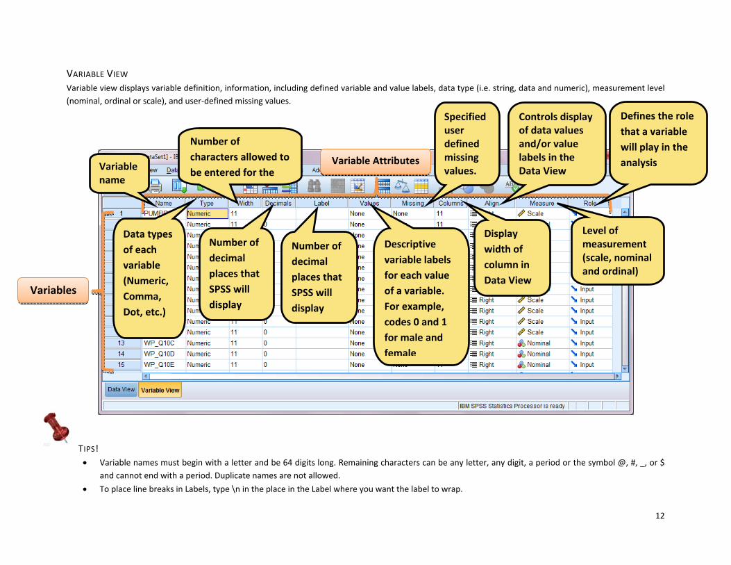
VARIABLE VIEW Variable view displays variable definition, information, including defined variable and value labels, data type (i.e. string, data and numeric), measurement level (nominal, ordinal or scale), and user‐defined missing values.

TIPS! Variable names must begin with a letter and be 64 digits long. Remaining characters can be any letter, any digit, a period or the symbol @, #, _, or $

and cannot end with a period. Duplicate names are not allowed. To place line breaks in Labels, type \n in the place in the Label where you want the label to wrap.

Variable Attributes

Variables

Level of measurement (scale, nominal and ordinal)

Specified user defined missing values.

Number of characters allowed to be entered for the Variable

name

Data types of each variable (Numeric, Comma, Dot, etc.)

Number of decimal places that SPSS will display

Number of decimal places that SPSS will display

Descriptive variable labels for each value of a variable. For example, codes 0 and 1 for male and female

Display width of column in Data View

Controls display of data values and/or value labels in the Data View

Defines the role that a variable will play in the analysis

13

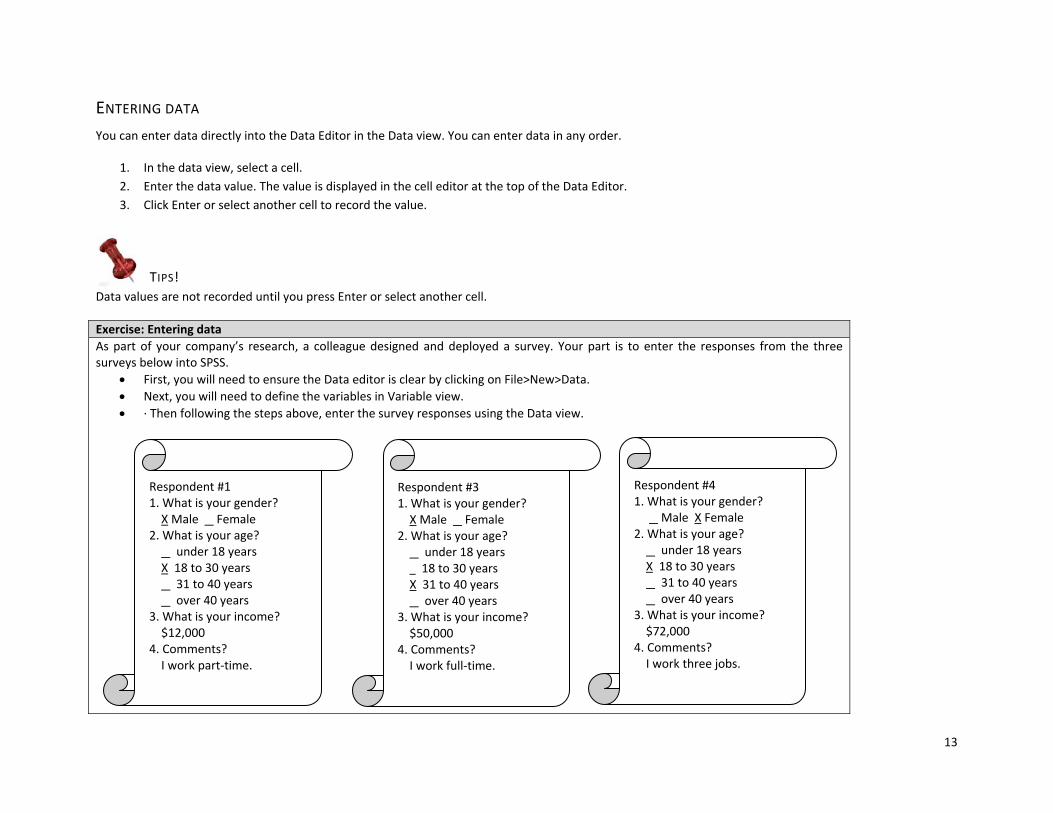
ENTERING DATA You can enter data directly into the Data Editor in the Data view. You can enter data in any order.

1. In the data view, select a cell. 2. Enter the data value. The value is displayed in the cell editor at the top of the Data Editor. 3. Click Enter or select another cell to record the value.

TIPS! Data values are not recorded until you press Enter or select another cell.

Exercise: Entering data As part of your company’s research, a colleague designed and deployed a survey. Your part is to enter the responses from the three surveys below into SPSS.

First, you will need to ensure the Data editor is clear by clicking on File>New>Data. Next, you will need to define the variables in Variable view. ∙ Then following the steps above, enter the survey responses using the Data view.

Respondent #1 1. What is your gender? X Male Female

2. What is your age? under 18 years X 18 to 30 years 31 to 40 years over 40 years

3. What is your income? $12,000

4. Comments? I work part‐time.

Respondent #31. What is your gender? X Male Female

2. What is your age? under 18 years 18 to 30 years X 31 to 40 years over 40 years


4. Comments? I work full‐time.

Respondent #41. What is your gender? Male X Female



4. Comments? I work three jobs.

14

INSERTING NEW VARIABLES Entering data in an empty column in the Data view or in an empty row in the Variable view automatically creates a new variable with a default variable name (the prefix var and a sequential number) and a default variable name (numeric).

You can also insert new variables between existing variables following these steps:

1. Select any cell in the variable to the right of the (Data view) or below (Variable view) the position where you want to insert the new variable. 2. Click Data>Insert Variable.

DELETING VARIABLES To delete a variable in the Data view (Variable view), right‐click on the variable name in the column (row) header and select Delete.

INSERTING NEW CASES Enter data in a cell on a blank row automatically creates a new case. The Data Editor inserts the system‐missing value for all the other variables for that case. Here are the steps to insert a new case between existing cases:

1. In the Data view, select any cell in the case (row) below the position where you want to insert the new case. 2. Click on Data>Insert Cases.

DELETING CASES To delete a case in the Data view, right‐click on the case number in the row header and select Delete.

MOVING TO A SPECIFIC CASE Suppose you have a large data set with about 10,000 cases and wish to see case 3,452. You would either manually scroll down to case 3,452 or use ‘Go to Case’ option. Here are the steps to using the ‘Go to Case’ option:

1. Make the Data Editor window active. 2. Click on Edit>Go to Case… 3. Type in the case number or row number you wish to see.

15

Exercise: Inserting a new case After you entered all the data, your colleague just gave you the survey for Respondent #2. Using the steps outlined above for inserting new cases, insert the Respondent #2 survey between case 1 and 2.

Respondent #2 1. What is your gender? X Male Female



4. Comments? I work full ‐time.

16

SYNTAX FILE Typically SPSS users read a data file into the Data Editor and then select items from the menus to manipulate the data or perform statistical analyses. This is referred to as interactive mode because the program provides a response each time you make a selection. For example if you request a transformation, the data set is immediately updated. If you select an analysis, the results immediately appear in the output window.

Alternatively, it is possible to work with SPSS in syntax mode, where the user types code in a syntax window. Once the full program is written, it is then submitted to SPSS to get the results. It is beneficial to have some programming knowledge when using syntax to produce the data transformations and analyses that you want. Generally, the interactive mode is easier and quicker if you only need to perform a few simple transformation or analyses on your data. Here are some situations when it would be better to use syntax over interactive mode:

Procedures and options are only available in the interactive mode. Expect to perform the same procedures on several different data sets and would like to save a copy of the code so that it can easily be re‐run. Need to perform a large number of similar transformations, such as using vectors and loops. Performing a very complicated set of procedures and it would be beneficial to document all of the steps leading to the results.

Each time a selection is made in interactive mode, SPSS records the syntax code in a “journal file”. The location and name of this file can be found/edited by clicking Edit>Options then click on the File Locations tab. If you ever want to see or use the code in the journal file, it can be edited in the journal file in a syntax window.

SPSS also provides an easy way to see the code corresponding to a particular menu function. Most selections include a Paste button that will open a syntax window containing the code for the function, including the details required for any specific options that you have chosen in the menus.

Exercise: Running a syntax file The excel file containing the data has been imported into SPSS. Now, we will open the syntax file containing the commands which will define the value labels and missing values for each variable. To do this click on File>Open>Syntax, then look for the syntax file Syntax1.sps and click on the “Open” button.

The Syntax Editor will open then select all the commands and click on the button.

17

SELECT CASES The Select Cases command excludes from further analysis all those cases that do not meet specified selection criteria.

Steps on how to Select Cases

1. Click on Data > Select Cases. 2. The following dialog box will appear:

Select Cases provides several methods for selecting a subgroup of cases based on criteria that include variables and complex expressions. You can also select a random sample of cases.

Output

18

DATA TRANSFORMATIONS

COMPUTING VARIABLES Compute Variable computes values based on numeric transformations of other variables.

You can compute values for numeric or string variables You can create new variables or replace the values of existing variables. For new variables, you can also specify the variable type and label. You can compute values selectively for subsets of data based on logical conditions. You can use more than 70 built‐in functions, including arithmetic functions, statistical functions, distribution functions, and string functions.

STEPS TO COMPUTE A VARIABLE 1. Click on Transform>Compute and the dialog box below appears

Available variables in working file.

Function List Over 70 built‐in functions exist.

Numeric Expression computes the value of the target variable. Just remember that string constants must be enclosed in quotation marks. Also, numeric constants must be typed in American format with the period (.) as the decimal indicator.

Type the name of a single target variable. It can be an existing variable or a new variable to be added to the The type and label for

the target variable can be modified by clicking this button.

19

2. In the text box labelled ‘Target Variable’, type in a variable name where the calculation result is to appear. It can be an existing or new variable name. If you choose to type in an existing variable, the values for this variable will be overwritten.

3. To build an expression (calculation), either paste components or type directly into the ‘Numeric Expression’ field. 4. If you wish the calculation in question be only applied to certain subset of the data, the If function is invoked. For example, you may want to increase

the salary for female by $100. To do this click on the ‘If’ button located at the bottom of the Compute Variable window shown above. The dialog box below appears and type :

TIP! Be careful what name you enter in the target variable field. If you enter in an existing variable name and go ahead with the transformation, the transformation cannot be undone, it is permanent.

Exercise: Computing Variable In this dataset we have a variable which represent the number of cigarettes a respondent smoked each day of a particular week. Let’s create a new variable (totcig) that represent the total number of cigarettes smoked by a respondent each week.

Specifies the condition that must be met for an observation to be included in a subset of data

Available variables in working file

20

RECODING VALUES You can modify data values by recoding them. This is particularly useful for collapsing or combining categories. You can recode values within existing variables or you can create new variables based on the recoded values of existing variables.

RECODE INTO SAME VARIABLES Recode into Same Variables reassigns the values of existing variables or collapses ranges of existing values into new values. For example, you could collapse salaries into salary range categories.

You can recode numeric and string variables. If you select multiple variables, they must all be the same type. You cannot recode numeric and string variables together.

STEPS TO RECODE VALUES OF A VARIABLE 1. Click on Transform>Recode>Into Same Variables and the following dialog box appears.


The variables to be recorded. All variables must be the same type (numeric or string).

21

2. Select the variables you want to recode. If you select multiple variables, they must be the same type (numeric or string). 3. Click on Old and New Values and specify how to recode values. The following dialog box appears.

TIP! Be careful what name you enter in the target variable field. If you enter in an existing variable name and go ahead with the transformation, the transformation cannot be undone, it is permanent.

Options to changenew values. Options to change

old values.

22

RECODE INTO DIFFERENT VARIABLES Recode into Different Variables reassigns the values of existing variables or collapses ranges of existing values for a new variable. For example, you could collapse salaries into a new variable containing salaryrange categories.

You can recode numeric and string variables You can recode numeric variables into string variables and vice versa. If you select multiple variables, they must all be the same type. You cannot recode numeric and string variables together.

STEPS TO RECODE VALUES OF A VARIABLE 1. Click on Transform>Recode>Into Same Variables, the following dialog box appears.

2. Select the variables you want to recode. If you select multiple variables, they must be the same type (numeric or string). 3. Enter an output (new) variable name for each new variable and click Change.

Specifies the output variable that will contain the recoded values from the selected variable. It cannot exceed 8 characters.

Descriptive name for the output variables.

Specifies old values and the new values they will be recorded into.

The variables to be recorded. All variables must be the same type. (numeric or string)


23

4. Click on Old and New Values and specify how to recode values, the following dialog box appears.

Exercise: Recoding into Different VariablesWorking with the same file, recode the age variable into the following groups:

Group Ages1 15‐242 25‐343 35‐444 45‐545 55‐646 65‐747 75‐848 85 and over

Options to change old values.

Options to change new values.

24

SELECT CASES There are situations in which a researcher would like to select observations meeting certain conditions. The specified condition is an arithmetic or logical expression that generally consists of a sequence of operands and operators.

SPSS provides a function that allows us to isolate a sub‐set of cases in a data file. It is the Select Cases command that excludes from further analysis all those cases that do not meet specified selection criteria. When cases do not meet the selection criteria, they will be turned ‘off’ or filtered, much like missing values so that they are not counted in further analysis. Alternatively, filtering is for cases to be deleted so that only those cases that meet the selection criteria remain in the data file. Filtering is the default setting, and the one generally used since deleting cases is a fairly drastic step and should only be used when we wish to trim down a very large file.

STEPS TO SELECT CASES 1. Click on Data>Select Cases and following appears.

Exercise: Select a subset of data Create a subset of the data with only females aged 15‐44 yrs of age.

25

ANALYZING DATA

DESCRIPTIVE STATISTICS Descriptive statistics describe patterns and general trends in a data set. In most cases, descriptive statistics examine or explore only one variable at a time. However, correlation and regression analysis describe the relationship between two variables. Depending on the type of required descriptive statistics, SPSS offers four types of descriptive statistics procedures including Frequencies, Descriptives, Explore and Crosstabs.

FREQUENCIES The frequencies procedure provides statistical and graphical displays that are useful for describing categorical variables which take on a value that is one of several possible categories.

STATISTICS AND PLOTS Frequency counts, percentages, cumulative percentages, mean, median, mode, sum, standard deviation, variance, range, minimum and maximum values, standard error of the mean, skewness and kurtosis (both with standard errors), quartiles, user‐specified percentiles, bar charts, and histograms.

DATA Use numeric codes or short strings to code categorical variables.

ASSUMPTIONS The tabulations and percentages provide a useful description for data from any distribution, especially for variables with ordered or unordered categories. Most of the optional summary statistics, such as mean and standard deviation, are based on normal theory and are appropriate for quantitative variables with symmetric distributions. Robust statistics, such as the median, quartiles and percentiles are appropriate for quantitative variables that may or may not meet the assumption of normality.

26

STEPS TO OBTAIN FREQUENCY TABLES 1. Click Analyze>Descriptive Statistics>Frequencies, the below dialog box appears.

2. Select one or more categorical or quantitative variables. Optionally, you can:

Click Statistics for descriptive statistics for quantitative variables.

Click Charts for bar charts, pie charts, and histograms.

Click Format for the order in which results are displayed.

Exercise: Generating summary statistics for a categorical variable Generate summary statistics for the SEX variable.

27

DESCRIPTIVES The Descriptives procedure displays univariate summary statistics for several variables in a single table and calculates standardized values (z scores). It is useful when you want to quickly see summary statistics for interval or ratio variables, but not the frequency tables or graphics output.

STATISTICS Sample size, mean, minimum, maximum, standard deviation, variance, range, sum, standard error of the mean and kurtosis and skewness with their standard errors.

DATA This procedure is best suited to describe continuous variables which can take on any value in a scale. Use numeric variables after you have screened them graphically for recording errors, outliers and distributional anomalies.

ASSUMPTIONS Most of the available statistics (including z scores) are based on normal theory and are appropriate for quantitative variables (interval or ratio level measurements) with symmetric distributions (avoid variables with unordered or skewed distributions). The distribution of z scores has the same shape as that of the original data; therefore, calculating z scores is not a remedy for problem data.

28

STEPS TO OBTAIN DESCRIPTIVES

1. Click Analyze>Descriptive Statistics>Descriptives, the dialog box below appears.

2. Optionally, you can:

Select Save standardized values as variables to save z scores as new variables.

Click Options for optional statistics and display order.

Exercise: Generating summary statistics for a categorical variable Generate summary statistics for the totcig variable.

29

JOURNAL FILE All commands issued either from a syntax window or from a dialog box are recorded in a journal file. This file can be reviewed with a text editor. This file also records any error or warning messages generated by commands. To find the location of the journal file, click on Edit>Options then the following Options dialog box appears. Click on the File Location tab and the location of the Journal File is displayed. As well, the options to turn the journaling feature off or on can be specified. Along with specifying whether the journal file should be overwritten or appended when a new session begins. The default filename is spss.jnl.

This file is particular useful if you previously ran a statistical analysis and forgot how it was done. You can quickly look at the journal, copy the syntax of interest and run the analysis again.

Click on this tab to view/change Journal File settings.

30

WORKING WITH THE OUTPUT When you run a procedure, the results are displayed in a window called the Viewer. In this window, you can easily navigate to whichever part of the output that you wish to see. You can also manipulate the output and create a document that contains precisely the output that you want, arranged and formatted appropriately.

VIEWER Results are displayed in the Viewer. You can use the viewer to:

Browse results Show or hide selected tables and charts Change the display order of results by moving selected items Move items between the Viewer and other applications

The view is divided into two panes. The left pane of the Viewer contains an outline view of the contents. The right pane contains statistical tables, charts and text output.

Outline Pane Contents Pane

Double click a table to pivot or edit it.

Click to expand or collapse the outline.

Double click a book icon to show or hide an item.

31

SAVING OUTPUT The contents of the Viewer can be saved to a Viewer document. The saved document includes both panes of the Viewer window (the outline and the contents). The file will have the .spo extension and is only viewable using SPSS.

STEPS TO SAVING OUTPUT 1. Make the Viewer window active and click on File>Save 2. Enter the name of the document and click on Save. This file will have the .spn extension and can only be opened by SPSS for windows.

EXPORT OUTPUT Export output pivot tables and text output in HTML, text, Word/RTF and Excel format. It saves charts in variety of common formats used by other applications.

Steps to Exporting Output

1. Make the Viewer the active window (Click anywhere in the window). 2. Click on File>Export. 3. Enter a filename. 4. Choose the Export Format file type you wish to save the file in.

TIP! Clicking on File>Save, saves the file as a SPSS .spo which only SPSS can read. To ensure a computer without SPSS installed, export the output using the steps above.

32

PASTING OBJECTS FROM THE VIEWER INTO OTHER APPLICATIONS Select an object and paste it into another application such as MS Word.

STEPS TO PASTING OBJECTS IN OTHER APPLICATIONS 1. Select the tables and/or charts to be copied (Shift‐click or Ctrl‐click to select multiple items). 2. Select Edit>Copy Objects. 3. In the target application, from the menus choose: Edit>Paste.

33

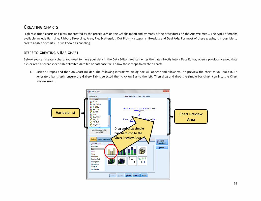
CREATING CHARTS High resolution charts and plots are created by the procedures on the Graphs menu and by many of the procedures on the Analyze menu. The types of graphs available include Bar, Line, Ribbon, Drop Line, Area, Pie, Scatterplot, Dot Plots, Histograms, Boxplots and Dual Axis. For most of these graphs, it is possible to create a table of charts. This is known as paneling.

STEPS TO CREATING A BAR CHART Before you can create a chart, you need to have your data in the Data Editor. You can enter the data directly into a Data Editor, open a previously saved data file, or read a spreadsheet, tab‐delimited data file or database file. Follow these steps to create a chart:

1. Click on Graphs and then on Chart Builder. The following interactive dialog box will appear and allows you to preview the chart as you build it. To generate a bar graph, ensure the Gallery Tab is selected then click on Bar to the left. Then drag and drop the simple bar chart icon into the Chart Preview Area.

Variable list Chart Preview Area

Drag and drop simple bar chart icon to the Chart Preview Area

34

2. A template of a simple bar chart will be shown in the Chart Preview Area. the Element Properties window appears, it assigns the properties to each of the chart elements. Drag and drop the independent variable (SEX) from the variable list into the “X‐Axis?” box in the Chart Preview Area. As well, drag and drop the dependent variable from (PS_Q40) the variable list into the “Y‐Axis?” box. Under Statistics select Mean.

Drag and drop variables to either the x or y axis.

35

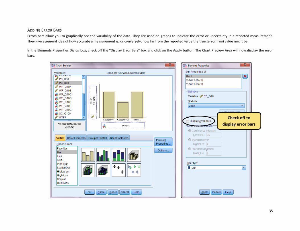
ADDING ERROR BARS Errors bars allow you to graphically see the variability of the data. They are used on graphs to indicate the error or uncertainty in a reported measurement. They give a general idea of how accurate a measurement is, or conversely, how far from the reported value the true (error free) value might be.

In the Elements Properties Dialog box, check off the “Display Error Bars” box and click on the Apply button. The Chart Preview Area will now display the error bars.

Check off to display error bars

36

MODIFYING AXIS LABEL The Axis Label can be edited by selecting the element in the “Edit Properties of” list box and then enter the text in the Axis Label text box.

Select element to modify.

Edit text to appear in graph.

37

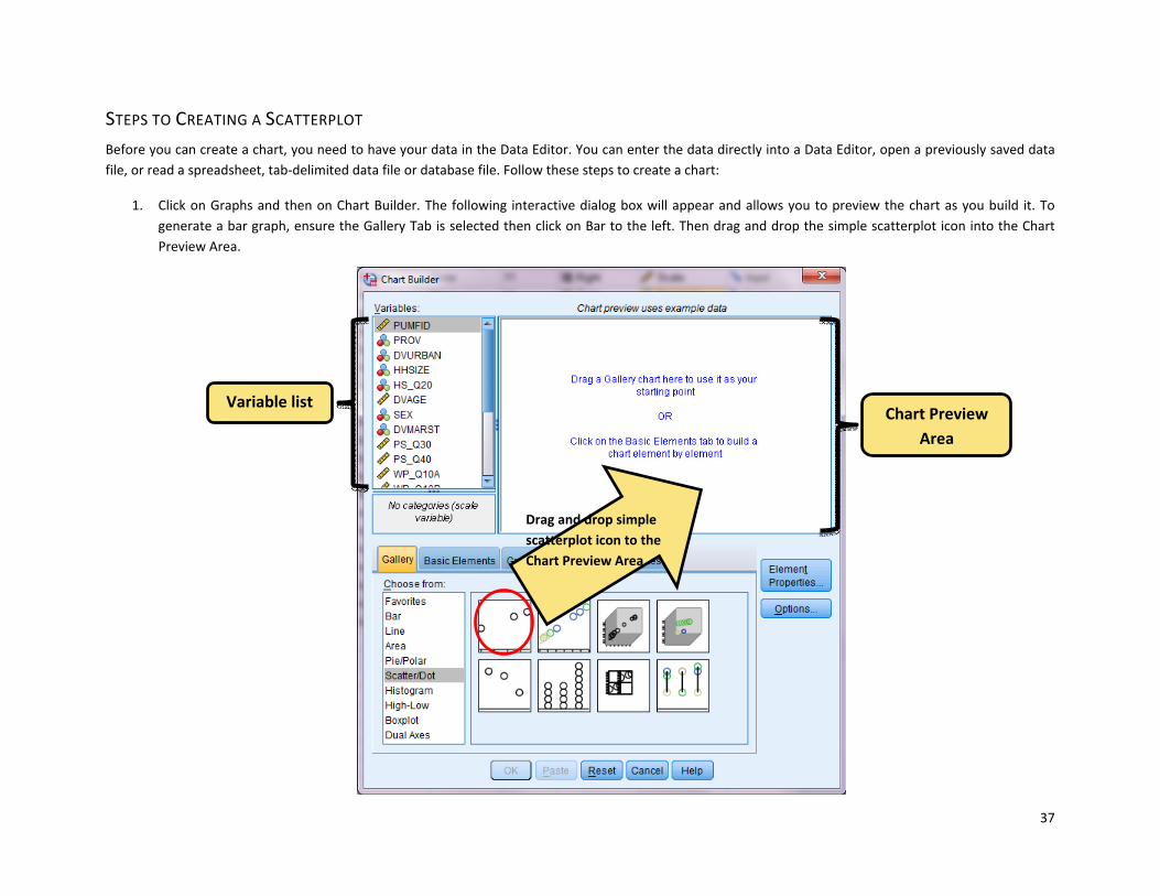
STEPS TO CREATING A SCATTERPLOT Before you can create a chart, you need to have your data in the Data Editor. You can enter the data directly into a Data Editor, open a previously saved data file, or read a spreadsheet, tab‐delimited data file or database file. Follow these steps to create a chart:

1. Click on Graphs and then on Chart Builder. The following interactive dialog box will appear and allows you to preview the chart as you build it. To generate a bar graph, ensure the Gallery Tab is selected then click on Bar to the left. Then drag and drop the simple scatterplot icon into the Chart Preview Area.

Variable list Chart Preview

Area

Drag and drop simple scatterplot icon to the Chart Preview Area

38

2. A template of a simple bar chart will be shown in the Chart Preview Area. the Element Properties window appears, it assigns the properties to each of the chart elements. Drag and drop the independent variable (DVAGE) from the variable list into the “X‐Axis?” box in the Chart Preview Area. As well, drag and drop the dependent variable from (totcig) the variable list into the “Y‐Axis?” box.

Drag and drop variables to either the x or y axis.

39

MODIFYING A CHART To modify a chart, double‐click anywhere on the chart that is displayed in the Viewer. This displays the chart in the Chart Editor. Any part of the chart can be modified or changed by clicking on the item of interest.

The most commonly edited part of a chart include the colour scheme, formatting number in the tick labels, editing text and data value labels.

CHANGING COLOURS 1. Double click on the bar chart to open it in the Chart Editor. 2. Click on any of the vars and rectangles will appear around the bars to indicate that they are selected. 3. On the Menu bar select Edit>Properties. 4. Choose the Fill & Border tab from the Properties Dialog Box 5. Click on the colour you wish. 6. Click Apply when the editing is complete.

FORMATTING NUMBERS IN TICK LABELS 1. If you are not in the Chart Editor mode then double click the bar chart. 2. Click on the y‐axis tick labels. 3. On the Menu bar select Edit>Properties. 4. Click on the Number Format tab. 5. Make the changes according then click Apply when the editing is complete.

EDITING TEXT 1. To make any text changes, you must be in the Chart Editor mode. 2. Double‐click on any of the titles you wish to edit. When in text editing mode, a flashing red bar cursor will appear. 3. Once the changes are complete press Enter to update the text.

getting your data into spss s11 - university of guelph · getting your data into spss ... to view...

Documents