Getting the inputs right for improved agricultural productivity in Madagascar, Which inputs matter and Are the poor different?1

by Claude Randrianarisoa

Cornell University and FOFIFA

and

Bart Minten Cornell University

June 2005

1 Paper presented during the workshop “Agricultural and Poverty in Eastern Africa” June 2005, World Bank, Washington D.C. ISSN 1936-5071 1

2

Getting the inputs right for improved agricultural productivity in Madagascar, Which inputs matter and Are the poor different?2

By Claude Randrianarisoa and Bart Minten

1. Introduction An improvement in the productivity of staple food crops could be a powerful way to alleviate rural - as well as urban - poverty in Madagascar (chapter 4 & 6). However, the crucial question remains on how to go about it. In this study we focus on the determinants of the productivity of rice, the main staple, based on recently collected household data from the central highlands and communal data for the country as a whole. The purpose of this analysis is twofold. First, we want to improve the insights in the determinants of rice production in Madagascar. Second, we link rice productivity and its determinants with poverty levels and study to what extent constraints, use and returns to factors of production differ by poverty levels.

The contribution of the chapter is multiple. First, we do one of the first analyses of panel data on rice productivity in Madagascar. By using recently collected data at the plot level, we are able to control for plot and household fixed effects which allows us to better evaluate the net effect of changes in the input allocation on the production of the plot. Second, we make explicit linkages between input use, agricultural productivity and poverty indicators. Third, we combine different datasets and methodologies - qualitative information, panel data analysis, spatial analysis and willingness to pay for inputs - to evaluate agricultural input and poverty linkages.

The structure of the chapter is as follows. First, the data and methodologies that will be used for the analysis in this chapter are presented. We then present a literature review of previous studies on rice productivity in Madagascar. In the fourth section, we look at descriptive statistics of the datasets at the household as well as the communal level. In section five, we discuss the self-reported qualitative statements on constraints on agricultural productivity by agricultural households and rural communities. Section six presents the quantitative analysis, using production function analysis at the household level and comparing differences in yield and improved technology adoption at the communal level. Then we use willingness-to-pay questions in section seven to evaluate the demand for two important agricultural inputs, chemical fertilizer and irrigation, with important policy relevance in Madagascar and that are high on the list of priorities by poor farmers. We finish with the conclusions.

2 Paper presented during the workshop “Agricultural and Poverty in Eastern Africa” June 2005, World Bank, Washington D.C.

3

2. Data and methodology 2.1. Data description We base ourselves on two types of data, spatial communal data and household level data. First, we rely on the commune census of 2001 and the commune survey of 2004. This allows us to use mapping techniques to show spatial adoption of specific agricultural technologies. It also allows us to give a rare picture of the variation at the national level as all communes were visited in 2001. A detailed description of the 2001 survey is given in the previous chapter. In 2004, a communal survey was organized in 300 rural communes, financed by the World Bank. Subjective questions on the situation in the agricultural sector were included and are used in the qualitative analysis section (section 5). Second, for the household level analysis, we base our quantitative and willingness-to-pay analysis on two rounds of household data implemented in 2002 and 2003 and both financed by the Basis Crsp project of Cornell University. Both surveys were conducted during the off-season period, three to four months after the main rice harvest. The surveys were done in two different regions in the highlands of Madagascar: the Vakinankaratra region and the rural communes surrounding the city of Fianarantsoa, referred to as Fianarantsoa II. Farmers in both areas are known to have a long experience in rainfed and irrigated rice production. Villages were randomly selected based on a stratified sample set-up. The strata were chosen based on the size of the village itself (large and small) and the distance to a paved road (close, medium and far).3

The 2002 data were gathered through a comprehensive survey collecting information at the plot and household level. The same farmers were visited in 2003 as in 2002 and the structure of the 2003 questionnaire is similar to the 2002 one. However, the 2003 survey was solely focused on rice productivity and was also linked with a soil analysis survey. Almost all of the initially interviewed households could be retrieved in 2003. The main reason for not retrieving households was a short-term absence in the village because of social obligations or temporary migration (mostly for agricultural wage labor as well as labor in mines). In two cases, households refused to be interviewed. Three households migrated permanently. As one of the objectives of the paper is to look at the linkages between poverty and rice productivity, we use the households’ income in 2002, computed as the sum of the consumption and sales of agricultural commodities and livestock, and non-agricultural and wage income. While we acknowledge the well-known problems of using income data as a measure of welfare, it is the only welfare indicator at our disposal as the surveys were mainly focused on measuring agricultural activities and production. As we will use this income indicator to distinguish welfare levels, we assume that the measurement 3 Since our sample is based on a random stratified sampling frame done some years earlier, our panel data sample has a bias toward older and wealthier farmers compared to the actual situation in each village. The first sampling of these households for Vakinankaratra was done in 1992 (Zeller, 1993). The initial Fianarantsoa households were chosen during the IFPRI project in 1997 (Minten and Zeller, 2000).

4

errors as well as inter-annual variability (we will divide households in 2003 also based on the income data of 2002) would not severely affect the outcome of the analysis. Finally, in the qualitative section, we also rely on the household data of the national household surveys of 2001 and 2004 (see chapter 3). Given that the qualitative sections on constraints to agricultural and rice productivity were worded similarly in these household surveys as in the BASIS CRSP survey and the commune survey of 2004, it allows us to confront the results of different surveys, methodologies and samples. 2.2. Spatial data analysis To explore the key determinants of agricultural productivity in Madagascar while controlling for biophysical conditions, we regress rice yields on land quality, labor inputs, stocks of livestock, mechanical and infrastructure capital, an index of farmer adoption of land intensification technologies, and climatic shocks. Technology adoption might be endogenous, with farmers choosing to adopt better technologies on better soils, in communes with better extension agents, and where higher ex ante yields generate surpluses that farmers plough back into the adoption of these technologies. We therefore tested for endogeneity using a Davidson-MacKinnon test. The index of farmer adoption of land intensification technologies was constructed as simple weighted sum of the adoption of SRI, fertilizer, improved seeds and transplanting. We also analyze the determinants of the adoption of agricultural technologies spatially. Given that we only have discrete categories for the number of people that adopt, we rely on ordered probit models. We analyze the adoption of six improved agricultural technologies: inorganic fertilizer, off-season crops, transplanting, improved rice seeds, SRI, and agricultural equipment (such as plows and harrows). The non-policy regressors include provincial dummy variables, temperature, altitude, soil variables, ethnic groups and climatic risks. The policy variables we include are literacy rates, access to irrigation, distance to extension agents, remoteness – which reflects travel time, not just distance – security and land titling. In the case of the yield regression, we correct for potential spatial autocorrelation as described in Conley (1999). We are not aware of a methodology to correct for spatial autocorrelation in ordered probit models. This was thus not done. 2.3. Panel data analysis Economic researchers often prefer to use panel data to study economic relationships. As fixed variables related to the community and household (and in our case plots) - which are often very difficult to measure – can be ignored, the analysis can better be focused on the evaluation of the effect of time-specific factors and the likelihood of contamination of estimated effects on input variables is reduced. The obvious drawback is that the returns to these fixed inputs can not be evaluated. The methodology is explained below in more detail.

Assume that there are t periods of time corresponding to t different years of production. A production relationship can be written as follows:

5

yit = α + β xit + λzit + θi + µit (1)

where yit is the production level of plot i at time t; α is the intercept; β and λ are coefficient estimates for each factor of production; xit is a vector of variable inputs use at time t for plot i; zit is a vector of exogenous shocks at time t for plot i; θi is a vector of plot and household fixed effects; µit is the error term. By differencing over time, the effect of plot and household fixed effects are dropped and the relationship to be estimated can be written as follows: Δyit = Δβ xit + λΔzit + Δµit (2) Input allocations are choice variables, based on unobservable factors that would influence the level of production. Even after differencing, these are still time dependent decisions that would alter farmers’ decision on input allocation. This will especially be the case in our specification with labor. We therefore use instrumented labor use for the regression estimation. Labor, both hired and family is assumed to be a function of family size and family composition, households’ agricultural assets such owning of plow and oxcart, access to draught oxen, participation in non-agricultural activities or wage earning activities. The timing of application of chemical fertilizer, at the very beginning of the rice cultivation justifying the use of the actual amount of mineral fertilizer use , since this is exogenous to any event that may occur during the agricultural season , and indeed plot, farm, and farmer’s heterogeneity were purged out by the use of fixed effect technique. For manure and animal traction, we use the number od zebu, cow and draught oxen as a proxy since manure is barely traded in the area os study and the possession of draught oxen will determine the access to animal traction. One of our objectives in this chapter is to look at the difference in return to factors of production for different groups of households, categorized by relative poverty. We use the parameters estimated in the above model to predict the marginal physical productivity (MPP) of each factor, computed at the average value for each welfare group. To be able to allow the slope of the marginal return to change depending on the level of use of other factors, it requires the use of a functional form not linear in inputs. In this analysis, we use the quadratic form. For a more detailed discussion on production functions and functional forms, see annex 1 and 2.

2.4. Willingness-To-Pay (WTP) analysis A Willingness-to-Pay (WTP) question was included to estimate both irrigation and fertilizer demand. The scenarios that were presented are shown in annex 3 and 4. In the improvement of irrigation scenario, respondents were explained what the improvement would exactly entail. Before going to the valuation part, farmers were asked what they thought the effect would be on their fields. Given the potential of free riding and yea-saying, respondents were reminded that if they would underestimate what they would be willing to contribute, there would not be enough finance to make this a viable scheme. On the other hand, if they would state an amount that is higher than what they would be able to contribute, the irrigation scheme could not be sustained. Then, a specific amount

6

of contribution towards the operation and the maintenance of the irrigation scheme was offered which the respondent could accept or refuse (or express uncertainty). In the case of the fertilizer use, farmers were first asked if they thought fertilizers were beneficial for agricultural production. They were further asked on their knowledge of application rates as well as the prices in their region. Then they were presented with a scenario (see annex 4 for the exact wording). In line with the environmental economics literature, the recommended Dichotomous Choice (DC) format question was used (Arrow et al., 1993; Mitchell and Carson, 1989).4 The respondent was offered the opportunity to accept the bid at one of 8 randomly assigned prices. In the case of the irrigation improvement, if the person answered ‘yes’ to the bid, he was asked to specify how he would pay for these expenditures. Then, an extra question was asked on how sure he was about the functionality of such an irrigation scheme in his community. If the respondent answered negative in both cases, he was included in the refusal category. Uncertainty was also included in both cases in the refusal category. In the econometric analysis, the probability that a household said ‘yes’ to the bid is estimated as a probit model.5 With Y = 1 indicating yes, and Y = 0 indicating no, the probability of saying yes is estimated as :

P(Y=1) = Φ(x’b) (3)

where Φ is the standard normal distribution, x is a vector of explanatory variables and b are parameters to be estimated. The measurement and interpretation of the variables used as explanatory variables is straightforward. Most of the continuous variables were converted to a log form to reduce the effect of extreme values and to facilitate interpretation.

3. Literature review Rice is of large interest to policy-making in Madagascar and research on rice has thus been prominent. In this short review, we briefly synthesize the main results of the most recent economic research on the determinants of rice productivity. Irrigation is shown to have positive effects but they have been estimated to be less than generally expected and than in other countries. A weak response from access to improved irrigation infrastructure alone is generally found. Minten and Zeller (2000) found that irrigation, which is one variable used to control for land quality, had a significant and positive effect

4 The benefits and disadvantages of this method are well studied. The advantages of this method are: 1/ reveals more accurate values than in the open-ended format; 2/ Simplifies the task of the respondent; 3/ the DC method resembles better the market place and more truthful answers are therefore expected. The disadvantages are the need for a large sample, the need for good framing of the question to avoid yea-saying and starting point bias and assumptions about the error term in regression analysis that might affect the parameter estimates (Arrow et al., 1993; Mitchell and Carson, 1989). 5 The question on suitability of logit or probit models is unresolved. However, in most applications, it seems not to make much difference (Greene, p. 815).

7

on production, but its magnitude was relatively small. In a review on the impact of public spending on irrigated perimeter productivity over the last twenty years in Madagascar (World Bank, 2005), rehabilitated irrigation infrastructure is shown to increase paddy yields by 1 ton/ha. Jacoby and Minten (2006) find similar results in their survey in the Lac Alaotra area when they compare maille (modern irrigation) versus non-maille (traditional irrigation) plots. The impact of chemical fertilizer is found in most analysis to be largely positive. For example, Bernier and Dorosh (1993) who studied rice productivity relying on a household survey done in the central region, including the Lac Alaotra area, and the highland region found that chemical fertilizer affected rice production positively with a marginal physical return of 6.2 kg of paddy for one additional kg of fertilizer (the per hectare average rate of application was 90 kgs). Randrianarisoa (2001) and Randrianarisoa and Minten (2001) showed a significant marginal return of about 6 kg of paddy-rice per kg of fertilizer use. A comprehensive descriptive analysis on rice trade in the highlands of Madagascar that was conducted by a team of French and Malagasy researchers in 1999 (UPDR, 2000) on the other hand found that only organic fertilizer had a large significant impact on rice productivity but not chemical fertilizer. Estimates on the returns to labor vary widely. For example, UPDR (2000) found in the highlands of Madagascar that partial average labor productivity was around 10 kg of paddy per day. On the other hand, Randrianarisoa (2001) finds a difference between “hired and family” in the returns to labor. While the use of hired labor shows interesting return, family labor, is low, sometimes lower than the prevailing agricultural wage rate at the village level. Especially smaller farmers have lower labor productivity, resulting in poor incentives to increase rice production. Researchers also looked at the impact of environmental and institutional constraints on rice productivity. Minten and Zeller (2000) focused in their study on the impact of market reform on agricultural productivity. Using village level data, they show that villages that have the opportunity for land extensification have lower rice productivity. Randrianarisoa (2001) and Randrianarisoa and Minten (2001) indicated the importance of natural exogenous production risk (climatic shocks) on plot productivity and Stifel and Minten (2003) highlighted the importance of access to infrastructure and remoteness on rice productivity. Based on data from a rural observation network (ROR), Robilliard (1999) shows the overall low price elasticity of rice supply, probably due to the large importance of auto-consumption in rice production. She shows that price elasticities are significantly larger for those households that are selling for the market. These previous analyses have in common that they use cross-sectional household data to estimate rice production functions. There are some caveats in such an approach, most importantly due to imperfect measures of plot, household and community characteristics. This analysis aims to increase the level of reliability of the estimation of the determinants of rice productivity, by relying on a recently constructed panel data, as well as expand the analysis differently through the use of a nationally representative spatial dataset.

8

4. Descriptive statistics 4.1. Income, production and agricultural practices Average annual per capita incomes (that were only available in 2002) in our dataset vary significantly by quintile (Table 1), from almost 30,000 Ariary (equivalent of $25 US) for the poorest quintile to more than ten times as much for the richest quintile (quintile 5). As also found in the national household data (chapter 3), this difference is driven by relatively and absolutely more important off-farm income (off-farm income represents 54% of the richest quintile versus 30% for the poorest quintile) as well as a significantly higher agricultural income (almost eight times as high for the richest quintile). Total rice production increases monotonically by income level. The per capita paddy production level of the lowest quintile corresponds to 20% to 25% of the national average consumption of 110 kg of white rice per capita per year (UPDR, 2000).6 These households must then often complete own rice production with purchases, especially during the lean period, if they have the means. To further get at welfare and food security indicators, a question was asked on the length of the lean period, i.e. the period when households are obliged to eat less. The self-reported length of the lean period drops significantly between the poorest quintile (almost 6 months) compared with the richest quintile (almost four months).7 The descriptive data show that the length of the lean period, total rice production and agricultural income are highly linked in the rural highlands of Madagascar and they indicate the importance of own rice production on nutrition and overall welfare in these villages. Table 1 further shows that the poor households in quintile 1 own significantly less agricultural assets than in quintile 4 and 5. They have fewer cattle, less equipment (as measured by the ownership of weeders) and less land, both upland and lowland. This is in line with characteristics attributed by villagers themselves to poverty in the same region (Freudenberger, 1998). Poorer households cultivate less area in total and also have smaller plot areas. Total rice area is about twice as large for the wealthier households compared to the poorest ones.8 Table 2 shows the rice productivity level as well as the use of production factors by income level. As we found with the national household survey (chapter 3), we notice also here the existence of average yield difference between quintiles. The poorest households have average yields that are 22% to 35% lower than the richest quintile in 2002 and 2003 respectively. However, in this simple two-way table, it

6 UPDR (2000) observed an average daily consumption of 2.26 kg of white rice per household in the Highland area of Madagascar, corresponding to approximately 110 kg of white rice, or 170 kg of paddy-rice per capita per year. 7 We also calculated the correlation between our measure of income poverty and the national poverty line benchmark of $0.42 per day per capita (Razafindravonona et al, 2002; chapter 2). Almost 80% of the households in our sample fall below this line. This is thus similar to the national poverty number in rural areas in Madagascar, indicating that the composition of our sample might well reflect the overall national situation. 8 Cultivated plot area may change over time since farmers may decide not to cultivate the whole plot, or decide to grown different cultivars on the same plot. In our further regression analysis, we take this change in the cultivated area into account.

9

is unclear to determine if the difference is due to better agricultural practices or to better quality land. The average number of oxen at the household level is evaluated at a little bit over 2. However, 30 to 35% of the household do not own oxen at all. Richer households own significantly more. The number of oxen at the household level is an important production factor in agriculture activities for two reasons. First, it is an indication of the use of manure, as manure markets are quite limited in the area of the study. For example in 2002, only 7% of the users (corresponding to 5% of total quantity) reported to have purchased manure.9 Second, the number of oxen is an indication of the availability of animal traction on the farm.10 Measures on the incidences of flooding and droughts are further used to control for climatic effects on productivity. 11% and 8% of the plots were reported to suffer from flooding in 2002 and 2003 respectively. This compares to 15% and 13% of the plots that suffered from droughts. This confirms qualitative statements of farmers in the highlands who consider droughts a bigger problem than floods. Rich and poor households are hit almost equally by these disasters. In any case, flooding and droughts are considered two major problems on lowlands in Madagascar and make rice production in lowlands a risky undertaking compared to upland production (see chapter 1).11’12 Finally, the level of technology adoption shows few links with income levels. While the age of transplanted plants - an indication of the adoption of the SRI technology - does not show significant differences across income quintile, the poorest quintile however uses slightly more the technique of in-line transplanting. For example in 2003, 53% of the poorest quintile declared to use the in line transplanting technique compared to only 42% for the richest quintile. We also note some slight differences in the number of days allocated to perform transplanting or weeding tasks. For all plots, fertilizer use is low (0.10 kg per are in 2002, and 0.13 kg per are in 2003). This number is far below the average in Asian rice producing countries such as Vietnam or Thailand or in other African rice producing countries such Nigeria or Mali.13 This finding is consistent with previous studies as chemical fertilizers are rarely used on staple 9 Organic fertilizer can be obtained directly from manure fermentation or from collecting weeds and other organic matters. During the National Agricultural Extension Project (PNVA) in the mid-90, the extension service diffused the technique of composting. However, manure is required in order to get good compost, so very few people make compost without having oxen. 10 There is a strong correlation between the number of oxen and the number of draught oxen. Respectively for 2000 and 2002, the coefficients of correlation between these two variables are .51 and .49. 11 For example, official production statistics in 2002 show that a surplus of 200,000 tons of rice was attributed to a good year for rice production, which means adequate rainfall and little incidences of flooding and drought. 12 We noticed that exogenous natural shocks are closely correlated. It seems that a plot without irrigation control system will have high probability to be flooded (in case of heavy rain) as well as be affected by drought. In turn, flooding might cause sedimentation and increase the risk of plant diseases by spreading the pests from other plots. 13 Fertilizer uses for these countries are 2.7, 1.7, 1.0, and 0.9 kg per are of rice respectively for Vietnam, Thailand, Nigeria, and Mali (FAO website).

10

foods in Madagascar. If we compare plots that did receive mineral fertilizer and those which did not, the overall average increase of rice productivity from fertilizer use is 20% of plot production.14 This change corresponds to a surplus of rice yield of 4.5 kg per are, obtained from an average fertilizer use of 0.59 kg per are.15 Taking simple ratios of these numbers gives us an average return of 7.6 kg of paddy from 1 kg of fertilizer. Average returns to family labor were also calculated: for example in 2002, average labor productivity was 50% higher for richer households compared to poorer ones, varying from 1455 Ariary per day for the poorest group to 3370 Ariary per day for the richest group, with an average of 2456 Ariary per day for the whole sample (Table 2).16’17 Given the caveats of simple two-way tables, we will turn to a more complete production function analysis of the panel component of these data in section 6. 4.2. Technology adoption The Green Revolution - based on high rates of fertilizer application and use of improved rice seed varieties - underscored the importance of improved technology adoption for agricultural transformation and poverty reduction in Asia (David and Otsuka, 1994; Evenson and Gollin, 2003). Unfortunately, the Green Revolution bypassed Madagascar. Figures 1 to 5 illustrate the low level of and spatial variation in the adoption rates of key improved agricultural technologies: inorganic fertilizer, off-season crops, early rice transplanting, the System of Rice Intensification (SRI), and improved rice seeds. Figure 1 shows that chemical fertilizer use is strongly linked to road or sea access. 94% of Madagascar’s agricultural households do not use chemical fertilizer (Minten et al., 2003). Several reasons exist for this. First, fertilizers are bought during the lean season, when many rural households are hard hit by liquidity constraints. Second, fertilizer prices are prohibitively high for most farmers, especially relative to declining international commodity prices, as transport and other types of infrastructure in Madagascar have degraded, therefore reducing profitability of fertilizer use.18 Not only is chemical fertilizer use low in rural Madagascar, only 36% of agricultural households use organic fertilizer either (Minten et al, 2003). Uptake of improved rice seed is similar (Figure 2), as roughly 90% of farmers do not use improved varieties.19 Goletti et al. (1998) illustrate the considerable difference between improved seed performance in on-station trials and

14 Yield difference between users and non-users. 15 Application rate only for plot receiving fertilizer. 16 UPDR (2000) found an average return per day per family labor between 10,519 fmg (2104 ariary) to 17,289 fmg (3458 ariary) for transplanted rice in the highlands of Madagascar. 17 These average returns were computed from the gross margin i.e. total revenue minus input costs, then divided by the number of hours of family labor spent on the plot. Input cost includes hired labor, seeds, fertilizer and chemicals, cost of animal traction, but without the opportunity cost of family labor. 18 Goletti et al. (1998) estimate that fertilizer prices are 60% higher in Madagascar compared to Southeast Asia due to thin markets and high transportation costs to get the fertilizer to Malagasy ports. 19 However, as seeds take on local names, it can be difficult to distinguish between traditional and improved varieties. In any case, finding that seeds are not replaced by newer varieties with modern names is an indication of the lack of technological innovation.

11

in farmers’ fields. This suggests substantial untapped genetic potential for rice in Madagascar. Lack of technological progress in Malagasy agriculture is reflected not just in limited use of inorganic and organic fertilizers or of improved rice seed. It is also manifest in limited adoption of higher yielding rice cultivation practices. One finds four types of lowland rice cultivation in Madagascar20: direct sowing, manual transplanting, intensive external input use (SRA: système de riz améliorée) and intensive labor use with a suite of adjustments to traditional agronomic practices (SRI: système de riz intensive). Direct sowing has been practiced for centuries. Rice seedling transplanting began in response to increased land pressure (Le Bourdiec, 1972). Lowland transplanting systems are the most common under irrigated conditions and cover about 820,000 ha or almost 60% of total rice-cultivated area (World Bank, 2003), as reflected in Figure 3. Direct sowing is attractive because of the high return on labor, which is estimated to be two to four times higher than for traditional transplanting (Bockel, 2002). However, land productivity tends to be lower, making these systems particularly attractive where access to land is less problematic. SRA systems yield more rice per unit land but require access to external inputs, especially inorganic fertilizers, chemical herbicides and mechanized or animal traction. SRI, by contrast, uses no purchased inputs but relies instead on a suite of agronomic adjustments: very early transplanting and wide spacing of seedlings, frequent weeding, and controlling the water level to allow for the aeration of the roots during the growth period of the plant, i.e., no standing water on the rice field (Uphoff et al., 2002; Moser and Barrett, 2003; Barrett et al., 2004). SRI has been shown to increase yields sharply, from an average of 2 tons/ha to 6 or more (Uphoff et al. 2002, Barrett et al. 2004). Because it does not require purchased inputs and because it was developed indigenously in Madagascar (de Laulanié 2003), many observers presumed that SRI would disseminate quickly to all rice farmers, and would be particularly beneficial to poor smallholders (Uphoff et al., 2002). However, while it has shown great promise, adoption rates have remained very low (Figure 4) and disadoption has been high mostly due to lack of continuous agricultural extension, deficient water management, seasonal liquidity constraints and increased yield risk (Moser and Barrett, 2003; Barrett et al., 2004). Double rice cropping (i.e., two harvests per year) is rare in rural Madagascar. Le Bourdiec (1972) links the lack of double cropping to cold highlands winters (temperatures decrease to the freezing point in some areas) and to behavior in coastal areas. Lack of good water management also poses a major constraint for double cropping, as good drainage and irrigation are necessary in the rainy and dry seasons, respectively. As double cropping for rice is often infeasible, adoption of off-season crops - such as

20 There also exist two rainfed rice production systems: uphill (tanety) and slash-and-burn (tavy). Irrigated systems cover about 80% of rice-cultivated area. Slash-and-burn systems cover almost 150,000 ha or 10% of total cultivated area. Uphill rice cultivation makes up the remaining 10% or so (World Bank, 2003). Yields in these latter two systems are significantly lower than in irrigated systems, cumulatively accounting for less than ten percent of aggregate rice production in the country. We focus here on the irrigated subsector.

12

potatoes, tomatoes, barley and wheat – on rice fields has become a key to intra-annual income stabilization, increased incomes and higher rates of adoption of SRI in specific regions, such as the Vakinankaratra (Moser and Barrett, 2003). Off-season cropping (Figure 5) might actually improve rice productivity by reducing planting season liquidity constraints and due to the soil nutrient enhancing effects of both inorganic fertilizers commonly applied to off-season crops (sometimes through contract farming arrangements that provide inputs as in-kind credit secured by the crop in a market with few buyers) and crop residues left in the fields and incorporated into the soil (Le Bourdiec, 1972; De Laulanié, 2003). In short, adoption of improved agricultural inputs and technologies lags in Madagascar, with the consequence that rice yields remain well below potential output. We have already established that lower rice yields result in higher rates of poverty and food insecurity (chapter 4). The critical policy question is thus what factors most directly affect rice yields so that agricultural productivity policy can focus on those interventions most likely to reduce rural poverty. This will be analyzed in further sections. 5. Qualitative analysis Before we move to a discussion of quantitative analysis, we let the farmers themselves talk. In the national household survey of 2001, farmers were asked what they saw as the biggest constraints to improved agricultural productivity. The same question was asked in the national household survey of 2004, based on a different sampling frame and with a slightly bigger sample. They were given different reasons – but they were not completely the same for the two years - and had to rank them from ‘not important’ to ‘very important’. The results are presented in the upper part of Table 3. We ranked the different constraints based on the percentage of households that reported them to be ‘quite’ or ‘very’ important. It is interesting to note the largely consistent answers between the two surveys, three years apart and with a different sample. The constraints that were ranked first, third and fourth were the same in both surveys as were the two constraints that were ranked last. Access to agricultural equipment, access to cattle for labor and access to labor are ranked respectively first, second and fourth. These answers illustrate at the national level to what extent constraints to increase labor productivity are seen by the farmers themselves as the reason for low agricultural production. The second most important batch of reasons is linked with the incidences of different shocks, such as plant diseases, droughts and floods. 56%, 61% and 54% of the households report these constraints to be ‘quite’ or ‘very important’. Only in the third batch are constraints on access to land intensification technologies such as access to agricultural inputs or access to cattle for fertilizer. It is also interesting to note the constraints that are not considered to be important by agricultural households. They include insecure property rights and silting of land. While security in property rights is in general an important determinant for soil investment and thus higher productivity (Reardon and al., 1996; Feder and Feeny, 1991), it seems that in the rural areas of Madagascar, the land tenure situation is such that little land conflicts

13

exist that would make such investments risky. An alternative explanation might be that credit markets, that would allow for such investments, are imperfect or missing and might not be linked with better property rights. Silting of ricefields is often linked to deforestation but this might cause less production problem than is commonly assumed (Brand et al., 2003; Larson, 1993). The same qualitative questions were used as to get at the constraints for increased rice production more specifically. In the commune survey of 2004, focus groups in 300 communes were also given the choice between four categories, ranking from ‘not important’ to ‘very important’. In the 2003 Basis Crsp survey, one randomly selected rice plot was chosen for each household and a question was asked on what households considered as the main constraint to increased rice productivity on that particular plot. Households were asked to rank twelve types of potential constraints on the same scale. The answers given in the commune survey are largely consistent with the results of the national household survey. The biggest constraint is labor productivity. Second comes shock mitigation. Third is land intensification. Fourth and last is an improvement in land tenure security and silting of land. In both the household and community survey, irrigation is seen as a major constraint for increased rice productivity. 85% of the communal focus groups report that better irrigation is the most important constraint in having higher rice productivity. This compares with 81% in the household survey. When looking at the answers of the rice growers in the highlands (the Basis Crsp survey), it is remarkable to note the differences in the ranking of the constraints compared to the three other surveys. In this case, land intensification technologies get a much more important place than at the national level. Access to cattle for manure is ranked first and access to agricultural inputs such as fertilizer is ranked fourth. Both indicators of demand for land intensification technologies are ranked higher than the labor productivity constraints such as access to labor (fifth), access to agricultural equipment (sixth) and access to cattle for labor (seventh). Climatic shocks are also considered less important in the highlands of Madagascar, presumably because these areas are less hit by cyclones than coastal areas. When we confront these results with the data of the national household for the province of Antananarivo and Fianarantsoa highland only (where the Basis Crsp survey was fielded), the same trends show up, i.e. access to cattle for manure and access to inputs becomes then one of the top priorities21. So, these trends seem to be robust. The qualitative results thus show a high perceived heterogeneity in constraints to improved agricultural and rice productivity in the different areas of Madagascar which should best be taken into account in policy and project design. 6. Quantitative analysis 6.1. Panel data analysis Table 4 presents the estimation results from a regression linking the effect of the variation in input use over the two years of the Basis Crsp surveys with the variation of rice 21 Farmers in these sites practice high-value off-season cropping which requires lots of organic fertilizer.

14

productivity. Two specifications are presented, a regular regression and an instrumented specification as discussed in the methodology section. A fixed effect specification was preferred after comparison of random and fixed effect models.22 We test the null hypothesis that all the coefficients are equal to zero against the alternative that at least one coefficient is not zero. We report the result with the marginal productivities and elasticities for each factor with quantitative measurement and the shift in production for factors used as productivity shifters (climatic exogenous shock). Table 5 summarizes the elasticities and marginal productivities, computed at the sample mean and at the mean of each quintile of poverty (see Annex 2 for more details). The results show that agricultural labor input, fertilizer use, animal traction and use of manure, technology adoption, and plot specific climatic condition are all significant determinants of rice productivity at the conventional statistical levels. Total landholdind and total value of agricultural equipment did not show significant impact on rice productivity. We see strong and positive effects of technology use on rice productivity. Using the age of plant at the transplantation as a proxy to control for technology adoption, the results show a very strong responses by a decrease of 0.11 kg in yield per additional day. Reducing the average age of transplanting from 48 to 24 would result in an increase of 13% of rice productivity. By its direct effect of draft power for plowing and transportation and its indirect effect for manure supply, having more oxen and draught oxen would be expected to affect positively rice production. One additional cattle at the farm is expected to increase rice yield by 1.1 kg, while doubling the number of cattle available to agricultural farms would lead to an increase of 7.4% in rice productivity. Across quintile of income, richer households would benefit 30% more return than the poorer household. While the use of manure was widely reported to have significant positive effect on rice yield, other researchers found recently a non-significant yield difference from the use of animal traction or manual tools for plowing (UPDR, 2000). Labor has positive marginal physical returns. One additional hour of work would result in increase of 1.05 to 1.65 kg of rice yield (Table 5) depending on the level of households’ wealth. There is a net gradient from lower to higher of return to labor across the quintile of households’ wealth. Poor farmers get lower marginal return to labor, which may become an issue when considering rice production as a levier for poverty reduction. At the price of rice and price of fertilizer in 2002, this physical marginal return corresponds to a marginal value product of 1,680 Ariary23 for the poorest households, just 20% higher

22 Hausman (1978) suggested a test to check for the consistency and the efficiency of fixed effect estimators. Following Greene (1997), we assume the null hypothesis that there is no correlation between the independent variables and the individual effect is ui. Under H0, the fixed-effect approach gives consistent but inefficient results and a random effect approach should be used instead. With a computed chi2(27) = 105, we reject the null hypothesis at 1% level, indicating that the correlation between the independent variables and the individual plot effect is not zero and have therefore a preference toward fixed-effect estimation. 23 These marginal value products were computed from a 8 hours of work per day, and a price of paddy rice of 200 Ariary per kg.

15

than the prevailing wage rate at the site of the surveys, and to 2,640 Ariary for the wealthier households, almost two times higher than the agricultural wage rate. Rice production is further very sensitive to changes in climatic conditions in Madagascar. Respectively for the richest and the poorest households, the results show that yields may decrease by 4% to 13% due to lack or too much rain, with significant strng negative impact for the lowest two quintile of wealth (Table 5). For example by their limited ability to replace flooded plants or respond adequately to the effect of climatic shock by investing in more labor use, poorer farmers may become more vulnerable to idiosyncratic climatic shocks. Usually, difficulties in water control, timeliness of agricultural tasks, and heterogeneity of soil quality lead to the well-documented inverse relationship between landholding and productivity (Lamb, 2003; Feder, 1985; Bhalla and Roy, 1988; Benjamin, 1995) and in Madagascar (Barrett, 1996; Randrianarisoa, 2002). In this analysis, we fail to observe such case. The overall result shows that change in landholding does not affect rice productivity at all24, but when we look closely at the variation among quintile of wealth, it is interesting to notice that poorer farmers have negative return to an increase in landholding while wealthier farmers would be expected to be able to increase their rice yield by 2% from an increase of 10% of their landholding.. 6.2. Spatial analysis on the determinants of yields We further explore the determinants of agricultural productivity based on the communal dataset. As technology adoption might be endogenous, we tested for endogeneity using a Davidson-MacKinnon test. Somewhat to our surprise, this test does not reject the null hypothesis of exogeneity (Table 6). It seems that our biophysical and provincial controls adequately account for those potentially confounding factors. We therefore report the results of ordinary least squares estimation. For this analysis, we also constructed an adoption index, consisting of an average of the percentage of people in a commune that employ land productivity increasing technology, i.e., adoption of fertilizer, early rice seedling transplanting, improved rice seeds and a new system of rice intensification known as the système de riz intensive (SRI).25 The coefficient estimates (Table 6) show that an increase in the number of farmers who adopt improved land-intensification technologies increases rice yields significantly, controlling for all other inputs and biophysical attributes of the production systems. Access to improved equipment in the commune has a positive effect on rice yields, but only about half that of the overall land intensification technologies adoption index. Irrigation leads to higher uptake of improved technologies but also leads directly to higher rice output due to better water management. An improvement of the irrigation

24 Insignificant effect of 0.006 kg per are increase on rice yield. 25 SRI uses no purchased inputs but relies on a suite of agronomic adjustments: very early transplanting and wide spacing of seedlings, frequent weeding, and controlling the water level to allow for the aeration of the roots during the growth period of the plant, i.e., no standing water on the rice field (Uphoff et al., 2002; Moser and Barrett, 2003; Barrett et al., 2004).

16

system so that the whole commune would move from no irrigation to a system where all rice fields are hooked up to such a system would increase rice yields directly by an estimated 12%. These results underscore that staple crop yields respond to a range of production factors: advances in equipment and seed, better water management and improved land management practices. Each plays a role in advancing agricultural productivity, although not in equal measure. The number of livestock has a highly significant, positive effect on rice yields, even controlling for use of animal traction in field preparation. This likely reflects the benefits of organic fertilizers (manure) for soil structure and nutrient content. Organic fertilizer is often mentioned as one of the most important constraints for improved agricultural productivity in sub-Saharan Africa in general (Barrett, Place and Aboud, 2002) and Madagascar in particular (Freudenberger, 1998). Animal traction likewise has a statistically significant, positive effect on rice yields, demonstrating multiple pathways through which livestock positively affects crop agriculture in systems such as those found throughout rural Madagascar. 6.3. Spatial determinants of technology adoption As shown, adoption of land-intensifying improved technologies increases agricultural yields. We therefore further analyze the adoption of six improved agricultural technologies: inorganic fertilizer, off-season crops, early rice seedling transplanting, improved rice seeds, SRI, and agricultural equipment (such as plows and harrows). Table 7 presents ordered probit regressions to evaluate the determinants of adoption of each of these improved practices or inputs.26 The non-policy regressors include provincial dummy variables, temperature, altitude, soil variables, ethnic groups and climatic risks. The policy variables we include are literacy rates, access to irrigation, distance to extension agents, remoteness – which reflects travel time, not just distance – security and land titling. Most of the coefficient estimates conform to expectations. Access to improved irrigation infrastructure has a statistically significant, positive effect on adoption in almost all these regressions.27 This is not a surprising result. Access to improved irrigation infrastructure allows better water management and reduces the risk of investment in a new technology. It is clearly an important necessary – but not sufficient - initial condition to achieve agricultural transformation, as has been shown in other countries (Ravallion and Datt, 2002). However, the coefficient estimates are small indicating that irrigation alone will not stimulate rapid uptake of improved technologies. Along with irrigation, remoteness is the most consistent determinant of adoption of improved agricultural technologies. More remote communes have statistically

26 We use an ordered probit estimator because the dependent variable was recorded in one of five ordinal categories, ranging from 0 = no adopters, 1 = 1-25% farmers adopt the method, to 5 = 100% adopters. 27 Focus groups were asked to estimate the percentage of the rice fields that were irrigated by pumps, dams, rainfall or from a natural source. The first two variables were aggregated into a measure of access to improved irrigation infrastructure.

17

significantly lower likelihood of adopting each of the six technologies. This reflects both poorer information flow to more remote locations and weaker profit incentives for innovation in those communes that are less well integrated into the commercial trading system, thus facing higher input and lower output prices. The coefficient estimates are especially highly significant for technologies that have to be imported from abroad – such as chemical fertilizer - given that access to roads is a necessity. Other policy variables matter to technology adoption patterns as well, but less significantly or consistently than irrigation and remoteness. Lower illiteracy levels in the commune lead generally to significantly higher adoption rates. This is consistent with Randrianarisoa and Minten’s (2002) results, based on national household survey data. This is not unexpected given the notoriously low education levels overall in rural areas. Based on the 1993 data, 44% of the population is illiterate. Marginal benefits to extra levels of education thus appear quite high. On the other hand, Fraslin (2002) argues that most education in rural Madagascar is not geared towards agricultural knowledge and is therefore of little direct use to farmers. The presence of land titles has a mostly positive impact, statistically significant in a few cases, including the overall adoption index.28 However, we are unable to deal with an endogeneity problem in the commune-level data that results from the fact that the demand for titles is higher on better endowed land, i.e., on land close to cities or more fertile land. By contrast, Jacoby and Minten (2005), using household level data in a specifically designed survey to measure the impact of land titling, found very little effect of formal land titling on agricultural productivity, investments or land values in Madagascar. We therefore urge caution in interpreting this result in our estimations. Distance to extension agents is highly significant in the case of SRI adoption and early rice transplanting, which is one component of the SRI package of agronomic practices. Moser and Barrett (2003) similarly find that access to extension is extremely important for successful adoption of SRI in rural Madagascar. However, access to extension services has no statistically significant effect on adoption of any other agricultural technologies. Given the longstanding literature on induced innovation, the effect of population density on agricultural technology adoption is surprisingly small, negative, statistically insignificant or all three in each of the regressions reported in Table 7. Hayami and Ruttan (1985) argue that farmers search for technical alternatives that economize on the use of increasingly scarce factors of production and that exploit increasingly abundant factors. This would lead to relatively more land-intensification investments in areas with land pressure associated with higher population densities (Boserup, 1965; Ruthenberg, 1980; Pingali et al., 1987; Pender et al., 2001). However, other factors seem to limit the applicability of the induced innovation hypothesis in rural Madagascar as it relates to the uptake of land productivity increasing technologies. Given that land intensifying

28 Given the high percentage of declared titled land, there is seemingly confusion on the exact definition of titles by the focus groups, confounding ‘terres titrés’ with the local informal ‘petits papiers’ system. For a more detailed discussion, see Jacoby and Minten (2005).

18

technologies are not taken up in high density populated areas, these areas suffer significantly lower real wages (as shown in chapter 4). Finally, ethnic group identities have a statistically significant effect on technology adoption patterns, as well as on rice yields (Table 7). This is consistent with Le Bourdiec’s (1972) observations that different ethnic groups in Madagascar started off with quite different rice cultivation systems and that the time required for the adoption might differ by ethnic group due to cultural reasons. Physical and location characteristics likewise matter significantly to agricultural technology adoption, as manifest by the estimated coefficients on rainfall, the presence of volcanic and alluvial soils as well as the provincial dummies. To summarize this section’s results, agricultural productivity is, as one would expect, strongly and positively associated with the adoption of improved agricultural technologies, access to agricultural extension, the availability of irrigation and market access. The latter two variables have both direct and indirect effects – through induced technology adoption – on rice yields in rural Madagascar. The commune-level data from Madagascar therefore suggest these are perhaps the most potent policy levers available if one wants to improve agricultural productivity so as to reduce poverty and food insecurity.29 7. Willingness-to-pay analysis 7.1. Chemical fertilizer use Given the importance for policy purposes, we look more closely at chemical fertilizer use. Based on our panel data regression results, it is found that one additional kg of chemical fertilizer increases rice productivity significantly by 5.3 kg per are (Table 5).30 This represents the effect of total fertilizer use on rice production, i.e. nursery as well as the production plots.31’32 These estimates are consistent with previous work in this area (Bernier and Dorosh, 1993; Randrianarisoa, 2001; Randrianarisoa and Minten, 2001).

29 There are essentially two types of technologies: semi-irreversible ones such as investment in irrigation, leading to a permanent treadmill effect, and reversible ones such as the use of variable inputs (e.g., improved seeds and fertilizer), potentially leading to price fluctuations in the face of inelastic demand for food. In our estimates, effects of yields on welfare and prices have largely been identified from yield differences due to long-term investments, i.e., irrigation infrastructure (the key instrument). The argument carries through equally when yield increases are achieved through better farm practices or modern inputs. Yet, the costs of both technologies can be vastly different and are often borne by different agents, public investment in the case of large-scale irrigation versus farmers in the case of improved variable inputs. This topic deserves further research as it cannot be tackled with the cross-sectional commune census data, given the lack of information on costs/investments. 30 The 112 kg increase in Table 5 corresponds to a plot of 20 ares (average plot area at the sample mean). 31 It is a bit tedious to assess the exact marginal return for fertilizer use since for rice, most farmers use chemical fertilizer at the nursery plot. For example in the 2002 and 2003 surveys, only 11% and 16% of all plots have received fertilizer application compared to the 29% and 31% of plots receiving plants from nursery plots using chemical fertilizer. 32 The fertilizer users in the sample have an average application rate of 0.59 kg per are, amount weighted by plot area.

19

The marginal return is just below the average return of 7.6 kg of paddy per kg of fertilizer computed in section 4.3. We thus find a ratio marginal value product over factor price significantly greater than one. It is interesting to notice that poor farmers experience two times higher marginal return from chemical fertilizer than richer farmers (Table 5). To calculate the incentives for fertilizer use, we compare the ratio of the price of paddy over the price of chemical fertilizer (NPK) (Figure 6). To avoid incorrect inferences due to geographical factors, we only do this for the Lac Aloatra area for which we have data available and where prices for inputs and outputs are similar as for the highlands. The ratio shows large changes over years, with price ratios of paddy and fertilizer (NPK) varying between 2.6 and 7, the latter at the high of the presidential crisis. Using our estimated marginal return of 5.3 kgs of paddy for 1 kg of fertilizer, we also construct a ratio of the value of output over the cost of fertilizer. Over the five years that we have data, this value changed between 2.6 (in 2000) and 1 (in 2002). So, these results seem to indicate that fertilizer use on rice is profitable, i.e. if no uncertainty was involved. However, given the larger likelihood of flooding and droughts on ricefields, households might consider the risk for investment in fertilizer too high on these fields. This is illustrated by the evidence that households more easily use fertilizer on off-season crops than on ricefields.33 In an overview of fertilizer incentives in Africa, Yanggen et al. (2002) find that in order to be interesting for farmers in Sub Saharan Africa, the ratio of the value of output over the cost from fertilizer use should be at least 2, preferably 3. In the case of Madagascar, this ratio, as shown on Figure 6, was - for the years that we have data - only two years out of five higher than 2 but it never went over 3. This suggest that farmers in the highlands are on the borderline of profitability and it thus seems that the little use of fertilizer in general in Madagascar is partly driven by financial rational. The price ratios in Madagascar are in sharp contrast with other rice producing countries, especially those in Asia. For example, the current ratio of paddy over urea prices is 1.25 in India, less than half the lowest level that was noted in Madagascar over this five year period. This difference in ratios explains to a large extent why fertilizers are relatively little used in Madagascar compared to these other rice economies. The favorable ratio in Asian countries is due to the much lower prices of fertilizer, which is often locally produced and/or subsidized in many of these countries. Retail fertilizer prices in India (0,10$/kg), Vietnam (0.19$/kg) and Pakistan (0.14$/kg) are significantly lower than the prices that are practiced in rural areas in the Highlands of Madagascar (0.50$/kg). Different reasons might explain the relatively high price in Madagascar. Not enough fertilizer might be available due to recurrent state interventions and the disincentives for the private sector. The wrong fertilizer might also be used. The fertilizer most in vogue in 33 Claude Chabaud (a French agronomist with a long experience in the Lac Alaotra area) claims that even by using appropriate techniques (in line transplanting, water management, etc.), average yields of about 4,5 tons are routinely obtained in the Lac Alaotra area. To obtain higher yields, chemical fertilizer would be needed (personal communication).

20

Madagascar is NPK 11.22.16. However, DAP (Diamonimumphosphate) might be more appropriate as rice fields suffer less from K deficiency, especially in the Highlands (Rabeson, 2004). It is estimated that financial benefits could be considerable as this type of fertilizer is much cheaper. To further investigate the demand characteristics of the demand for chemical fertilizer, we rely on a willingness-to-pay analysis. A willingness-to-pay scenario for chemical fertilizer was presented to rural farming households in the 2003 survey. To introduce the scenario, the household was asked about the current use and the benefits of chemical fertilizer.34 Then the scheme was explained and the bid was offered. As shown in Figure 7 and Table 8, willingness to pay for fertilizer is quite responsive to price. For example, a price increase from 400 to 700 Ariary per kg would reduce the percentage of households willing to pay for fertilizer from 83% to 30%. Using the results of a parsimonious model where the acceptance dummy was regressed on an intercept and the logarithm of the price, median willingness to pay is estimated to be about 575 Ariary per kg. It is interesting to note that based on these willingness-to-pay answers, fertilizers would be used by almost all the farmers, independent of wealth, if prices were similar to those in East-Asian rice economies. A comprehensive model was then estimated including on top of the bid level, household characteristics, proxies for shocks over the last ten years, beliefs on fertilizer use and constraints on rice productivity and village dummies. The results (Table 8) illustrate the internal consistency in the answers by the households. Farmers that believe that fertilizer are beneficial for rice production, are more likely to accept the bid. Few other variables are significant. The more the household is involved in off-season crops, the more likely it will accept the bid, probably as profitability on these crops are higher. Older head of households are less likely to accept. No other variables came out significant.35 7.2. Irrigation An important intervention to reduce the risks of flooding and drought of rice plots and to increase the likelihood of the adoption of improved technologies, is the improvement of water management. It is estimated that 40% of Madagascar’s cultivated area is under some sort of irrigation (World Bank, 2003). Water management is therefore considered a key factor affecting agricultural sector performance. However, the government and the donors have grown wary of further investments in irrigation schemes given the mixed

34 Only two thirds of the households thought that the use of chemical fertilizer was beneficial on ricefields. This might underscore the need for extension to get out the message as how to use chemical fertilizer. 35 Caution is warranted in analyzing the potential of chemical fertilizer on total rice production in Madagascar. Since the current national consumption of fertilizer is very low, even a doubling of fertilizer use on rice would not affect significantly total rice production at the national level. Computed at an average return of 7.6 kg of paddy from 1 kg of fertilizer use, an increase of 10,000 tons of fertilizer use on rice would lead to an increase of 76,000 tons of paddy-rice production, roughly equivalent to 50,000 tons of milled rice, equivalent to approximately 2% increase of the total rice production, and equal to one fourth of the annual rice import for Madagascar for the last few years. To put it into an even more stark perspective, current fertilizer use would need to be increased at least by 25 times to be comparable to the Vietnam rice yield with the same technology.

21

results of past interventions (World Bank, 2005). This has mainly been due to an overemphasis on construction and a neglect of institutional issues. This has seemingly left few water user associations in place where sustainable payments of irrigation fees were collected and that were able to pay for operation and maintenance costs of these irrigation schemes (World Bank, 2003). There is currently little knowledge on what benefits and appropriate payment levels would be in a Malagasy environment.36 A Willingness-to-Pay question was therefore formulated and included in the survey of 2003: the results are used to evaluate the potential contributions of rice farmers to water user groups that would take care of operation and maintenance of the irrigation scheme. To introduce the scenario, the household was asked to enumerate the number of times the plot was hit by disasters such as floods, droughts, or late planting over the last ten years. The households were further asked to rank the different production constraints on the plot (as shown in Table 3). The irrigation improvement scenario was explained (see annex 3) and the household was then invited to evaluate to what extent it thought that this would affect rice productivity and to indicate in an open question the good and the bad effects of such an investment. Then, the bid was offered. As a close-out question, it was asked to the interviewees if they thought such a scheme could work in their community. The respondents who indicated that such a scheme would not work in their community ‘for sure’ although they accepted the bid, were reassigned to the refusal category. This category concerned 6% of the answers. A parsimonious and a comprehensive model were estimated to evaluate the importance of covariates for the willingness to contribute to irrigation maintenance (Table 9). A parsimonious model was estimated as a simple function of an intercept and natural log of the bid level. For the comprehensive model, the x vector included plot and household characteristics, the incidences of shocks over the last ten years on that particular plot, the perceived importance of different constraints on rice productivity and village dummies. The regressions were estimated using the Huber/White/sandwich estimator of variance in place of the traditional calculation. Figure 8 shows to what extent demand for irrigation infrastructure is responsive to price: a price increase from 200 to 500 Ariary per are per year would reduce the percentage of households willing to contribute to the water association from 60% to about 28%. This price effect is also reflected in the statistical analysis (Table 9). For both models, the coefficient on the bid level is negative and significant at the 1% level. Using the parsimonious model (without village dummies), median willingness to pay is estimated to be 161 Ariary per are per year. The median can easily be interpreted as the price level that would be rejected by 50% of the members of a community in a community vote. The results of the comprehensive model are presented in the last two columns of Table 9. The coefficient on income is significant and illustrates to what extent changes in poverty will lead to different demands for irrigation infrastructure. To illustrate the magnitude of

36 In our panel dataset, we did not observe any major change on the irrigation system between the survey years. Hence, an irrigation infrastructure variable/dummy is thus not appropriate to evaluate the benefits of irrigation.

22

the coefficient, we rely on graphical analysis (Figure 9). The Figure shows that if a low fee of 100 Ariary per year per are would be imposed, only 29% of the poorest quintile would be willing to accept to pay for it. This compares to 42% for the richest quintile. The other variables that turn out to be significant are the incidences of late planting due to lack of rain. Households that had more of these problems over the last ten years, are more likely to accept the bid. We also asked the household the highest and the lowest production that they achieved on the particular rice plot over the last ten years. The difference between these levels, an indication for risk, increases the probability of bid acceptance significantly. Households that consider lack of irrigation to be a main constraint on that particular plot were also more likely to contribute, illustrating internal consistency. Most farming households are convinced of the utility of improved water management schemes. They believe that it will lead to a significant increase of their rice productivity and of the cultivation of off-season crops. The median willingness to pay for such an intervention remains however surprisingly low – the median is evaluated at 13$/ha –. This is a small percentage of the presumed perceived actual benefits of outputs due to better irrigation. This low level might be due to interventions in the past where there was little cost recovery and investments were mostly taken care of by the state or by donors. It might also reflect distrust in the current functioning of water use associations. The level of the willingness to pay is also significantly below experiences in most other developing countries.37 Most importantly, this level is below actual costs: it has been estimated that the cost of proper operation and maintenance would be in the order of 23$ and $38 per hectare (World Bank, 2003). It seems therefore that induced formation of sustainable water user groups is difficult in Madagascar and it seems that Madagascar could learn from some successful experiences within Madagascar as well as in other developing countries.38 8. Conclusions As shown in the previous chapter, an improvement in the productivity of staple food crops could be a powerful way to alleviate rural - as well as urban - poverty in Madagascar. In this chapter, we study how to go about it. More in particular, we look at the determinants of the productivity of rice, the most important staple crop, based on recently collected micro-data and spatial data. We also make use of different methodologies: qualitative information, panel data analysis as well as WTP scenarios. While liberalization did not have the envisioned impact on rice productivity in Madagascar, this might be because the state seem to have abolished too much at once (especially irrigation) and sometimes not enough (as shown in their un-transparent interventions in fertilizer distribution). However, policy changes seem needed to improve 37 For example: Mali, Office du Niger: 85$ per ha; Egypt, Balaqtar: 32$ per ha; Mexico, Rio Yaqui ID 041: 45$ per ha; India, katerpurna: 7$ per ha, Waghad: 41$ per ha (World Bank, 2003). 38 For example, full operation and maintenance fees have been achieved in Mexico and in the "Office du Niger", Mali. In Mexico, they rely on an upfront payment system based on a volumetric basis. In Niger, farmers can be (and have been) evicted from their land in the case of non-payment of operation and maintenance fees (World Bank, 2003).

23

input supply in the agricultural production process as for example most Green Revolution success stories have been built on dynamic agricultural input markets (Dorward, 2004). Using qualitative statements of farmers out of different surveys, we find a consistent picture at the national level for a demand by farmers for labor productivity enhancing interventions, i.e. access to agricultural equipment, access to cattle for labor as well as improved irrigation. Shock mitigation measures, land productivity increasing technologies and improved land tenure are stated to be much less important. The qualitative statements also show differentiation by region. Farmers in the more densely populated highlands put access to manure and access to agricultural inputs such as fertilizer (as well as access to improved irrigation) highest on their list. These results are consistent with the induced innovation theory (Hayami and Ruttan, 1985) and indicate the need to avoid policies of ‘one size fits all’ for the country as a whole. Poorer farmers have lower rice yields than richer farmers and it is found that they would benefit relatively more from adoption of new technology on transplanting rice. It seems however difficult to target investments specifically to poorer farmers as increased production in rural areas would help the rural population as a whole through second-round effects (such as more active labor markets). This issue deserves more research. Using panel data from a small farmer survey in the highlands of Madagascar, it is shown that fertilizer use on rice is marginally profitable and that profitability shows large changes over years. Using willingness-to-pay scenarios, fertilizer demand is shown to be highly price sensitive. As the survey was conducted in one of the most accessible regions of Madagascar, this indicates that current fertilizer prices are out of reach for most farmers in Madagascar. Even in this accessible region, fertilizer prices were still at least three times as high as in the rice economies of Vietnam and Pakistan at the same period of the survey. It seems that a more rational structuring of the fertilizer supply chain, with clear and consistent market signals, might help at least the more accessible regions to more readily adopt chemical fertilizer. Irrigation schemes have over the years fallen in disarray in Madagascar as water user organizations did not have the capacity to organize themselves to manage the schemes properly (Droy, 1999; World Bank, 2003, 2005). However, unless these institutions function properly, internal rate of returns to irrigation are much lower (chapter 7). We find that while farmers are willing to pay for improved irrigation infrastructure through water use associations, the amounts they are willing to contribute are significantly below the costs - and significantly below international standards -, and this especially so for the poorest farmers. It is unclear why this is the case. Is it because farmers were used to have subsidized irrigation systems and they find it hard to change or is it because irrigation does not pay off? We tend to favor the former explanation as farmers clearly identify access to better irrigation as a major constraint to improved agricultural productivity. Some better understanding of how some of these water user associations did however succeed might help in the better and sustainable setting up of these organizations.

24

The results in this chapter indicate overall that there are no real magic bullets for better agricultural performance. Improved agricultural technology diffusion seems the most effective means of improving agricultural productivity and reducing poverty and food insecurity in rural Madagascar, but improved rural transport infrastructure, improved irrigation systems, maintenance of livestock herds, improved physical security, increased literacy rates and reasonable access to extension services all play a positive role in encouraging productivity growth and poverty reduction. None of these factors is easy to influence and all require a long-term commitment to agricultural and broader rural development.

References

Arrow, K., R. Solow, P.R. Potney, E.E. Leamer, R. Radner and H. Schuman (1993), Report of the NOAA Panel on contingent valuation, Federal Register, 58(10), 4601-4614. Barrett, C.B. (1996), “On Price Risk and the Inverse Farm size – Productivity Relationship,” Journal of Development Economics 51, 193-216. Barrett, C.B., F. Place, and A.A. Aboud, editors (2002), Natural Resources Management in African Agriculture: Understanding and Improving Current Practices. Wallingford, UK: CAB International. Barrett, C.B., C.M., Moser, O.V. McHugh and J. Barison (2004), “Better Technology, Better Plots or Better Farmers? Identifying Changes in Productivity and Risk among Malagasy Rice Farmers,” American Journal of Agricultural Economics 86 (4): 869-889. Benjamin, D. (1995), “Can Unobserved Land Quality explain the Inverse Productivity Relationship,” Journal of Development Economics 46: 51-84. Bernier, R. and P.A. Dorosh (1993), Constraints on Rice Production in Madagascar: The Farmer’s Perspective, CFNPP working paper 34, Cornell University Bhalla, S.S. and P. Roy (1988), “Misspecification in Farm Productivity Analysis: the Role of Land Quality,” Oxford Economic Papers 40: 55-73. Bockel, L. (2002), Review of Madagascar’s rice sub-sector, World Bank, Background report, Madagascar Rural and Environmental Review Boserup, E. (1965), The Conditions of Agricultural Growth: The Economics of Agrarian Change under Population Pressure, Chicago: Aldine Publishing Co. Brand, J., B. Minten and C. Randrianarisoa (2003), “Etude d’Impact de la Déforestation sur la Riziculture Irriguée,” Cahier d’Etudes et de Recherches en Economie et Sciences Sociales, FOFIFA, No. 6, 2002.

25

Conley, T.G. (1999), “GMM Estimation with Cross Sectional Dependence,” Journal of Econometrics 92: 1-45. David, C.C. and K. Otsuka (1994), Modern rice technology and income distribution in Asia, Boulder: Lynne Riener Publishers. De Laulanié, H. (2003), Le riz à Madagascar: Un développement en dialogue avec les paysans, Antananarivo : Editions Karthala. Diewert, W.E. (1971), “An Application of the Shephard Duality Theorem, A Generalized Leontief Production Function,” The Journal of Political Economy 79(3): 481-507. Dorward, A., J. Kydd, J. Morrison, I. Urey (2004), “A Policy Agenda for Pro-poor Agricultural Growth,” World Development 32(1): 73-89. Droy, I. (1997), “Que sont les Greniers à Riz Devenus? Le Désengagement de l’Etat sur les Grands Périmètres Irrigués de Marovoay et du Lac Aloatra,” Economie de Madagascar 2: 63-88. Evenson, R. and D. Gollin, “Assessing the Impact of the Green Revolution: 1960 to 2000,” Science 300 (2 May 2003): 758-762. Feder, G. (1985), “The Relation between Farm size and Farm Productivity: the Role of Family Labor, Supervision and Credit Constraints,” Journal of Development Economics 18: 297-313. Feder, G. and Feeny, D. (1991), “Land Tenure and Property Rights: Theory and Implications for Development Policy,” World Bank Economic Review 5:135-153. Fraslin, J. (2002), “Quel Avenir pour le Paysans de Madagascar?,” Afrique Contemporaine Trimestriel no 202-203: 75-92. Freudenberger, K. (1998), Livelihoods without Livestock: A study of Community and Household Resource Management in the Village of Andaladranovao, LDI, Madagascar. Goletti, F., C. Randrianarisoa and K. Rich (1997), “How Good is Rice Seed in Madagascar? The Structure and Performance of the Seed Sector”, in Part 2, Final Report, IFPRI-FOFIFA project, pp. 15-71 Greene, W. H. (1997), Econometric Analysis, Upper Saddle River, NJ: Prentice Hall. Hayami, Y. and V. Ruttan (1985), Agricultural Development: An International Perspective. Baltimore: Johns Hopkins University Press.

26

Hausman, J. (1978), "Specification Tests in Econometrics," Econometrica 46: 1251-1271. Jacoby, H. and B. Minten (2005), Is land-titling in Sub-Saharan Africa cost-effective? Evidence from Madagascar, mimeo. Lamb, R.L. (2003), “Inverse Productivity: Land Quality, Labor Markets and Measurement Error,” Journal of Development Economics 71: 71-95. Larson, B.A. (1993), “Changing the economics of Environmental Degradation in Madagascar: Lessons from the National Environmental Action Plan Process,” World Development 22(5): 671-689. Lau, L.J. (1972), “Profit Functions of Technologies with Multiple Inputs and Outputs,” Review of Economics and statistics 54(3): 281-289. Le Bourdiec, F. (1974), Hommes et paysages du riz à Madagascar. Antananarivo: FTM. Minten, B. and M. Zeller (2000), Beyond Market Liberalization: Welfare, Income Generation and Environmental Sustainability in Rural Madagascar, Vermont: Ashgate. Minten, B., L. Randrianarison and C. Randrianarisoa (2003), Agriculture, Pauvreté rurale et politiques économiques à Madagascar, Antananarivo: Cornell University/FOFIFA/INSTAT. Mitchell, R.C. and R.T. Carson (1989), Using Surveys to Value Public Goods: the Contingent Valuation Method, Washington DC: Resources for the Future. Moser, C. and C.B. Barrett (2003), “The Disappointing Adoption Dynamics of a Yield-increasing, Low External Input Technology: the Case of SRI in Madagascar,” Agricultural Systems 76(3): 1085-1100. Pender, J., S.J. Scherr, and G. Duron (2001), “Pathways of Development in the Hillside Areas of Honduras: Causes and Implications for Agricultural Production, Poverty and Sustainable Resource Use,” in Lee, D.R., Barrett, C.B., Tradeoffs or Synergies? Agricultural Intensification, Economic Development and the Environment, CABI publishing: 171-196. Pingali, P., Y. Bigot and H.P. Binswanger (1987), Agricultural Mechanization and the Evolution of Farming Systems in Sub-Saharan Africa. Baltimore: Johns Hopkins University Press. Rabeson, R., Le point sur la gestion de la fertilité des sols des rizières aquatiques des Hautes Terres de Madagascar, mimeo.

27

Randrianarisoa, J.C. (2001), The effects of Land Quality and Natural Shocks on Land and Labor Productivity on Rice in Madagascar’s Highlands, Michigan State University, Ms Thesis. Randrianarisoa, J.C. and B. Minten (2001), Agricultural Production, Agricultural Land and Rural Poverty in Madagascar. Mimeo. Antananarivo: FOFIFA/Cornell University. Razafindravonona, J., D. Stifel and S. Paternostro (2001), Changes in Poverty in Madagascar: 1993-1999, World Bank Africa Region Working Paper Series, No. 19. Washington, DC. Reardon T., Kelly V., Crawford E., Jayne T., Savadogo K., Clay D. (1996), Determinants of Farm Productivity in Africa: A synthesis of Four Case Studies. MSU International Development Paper No 22, Michigan State University, 1996

Robilliard, A.S. (1999), “L’Offre de Riz des Ménages Agricoles Malgaches: Etude Econometrique à Partir d’Enquêtes Transversales,” Economie de Madagascar 4: 265-284. Ruthenberg, H. (1980), Farming Systems in the Tropics, Oxford: Clarendon Press. Stifel D. and B. Minten (2003), Costs and Agricultural Productivity: Implications of Isolation for Rural Poverty in Madagascar. Mimeo. IFPRI. Uphoff, N., E. Fernandes, Y. Longping, P. Jiming, S. Rafaralahy and J. Rabenandrasana (2002), “Assessments of the System of Rice Intensification,” Proceedings of an international conference, Sanya, China, Cornell International Institute for Food, Agriculture and Development. UPDR – FAO (2000), Diagnostic et Perspectives de la Filière Riz à Madagascar Rapport, Antananarivo : Ministère de l’Agriculture, Unité Politique de Développement Rural (UPDR) FAO-CIRAD. World Bank (2003), Review of the Agricultural and Environmental Sector in Madagascar, Antananarivo: World Bank. World Bank (2005), Madagascar: The Impact of Public Spending on Irrigated Perimeters Productivity (1985-2004) Yanggen, D., V. Kelly, T. Reardon and A. Naseem (1998), Incentives for Fertilizer Use in Sub- Saharan Africa: A Review of Empirical Evidence on Fertilizer Yield Response and Profitability, MSU International Development Working Paper No 70, East Lansing: Michigan State University.

28

Zeller, M. (1993), Credit for the Rural Poor: Country Case Madagascar, Final Report to German Agency for Technical Cooperation, Washington DC: International Food Policy Research Institute.

29

Annex 1: The production function approach We will implement a model that explains observed production, as a function of biophysical characteristics of farmer’s choices and exogenous natural shocks. The use of the primal approach - which involves a maximization of an objective function (utility) subject to physical constraints such as land, labor, capital, and other exogenous variables - is justified for two reasons. First, as farmers make decisions on input uses prior to realization of input or output prices, the observed prices are almost surely not the ones over which farmers made their inputs decision. Second, it has been argued that the production function approach is as prone to endogeneity bias as profit function analysis as prices at the farm level are endogenous (Barrett et al., 2003). The production function can be written as follows: yi = f(x1 … xm), i = 1 to n, and where yi is the output for plot i, and (x1 … xm) a vector of inputs quantities. We assume that xi ≥ 0 and finite for all i from 1 to m, where m is the number of inputs. We further assume also the production function is concave, implying the properties of diminishing marginal return of each factor of production. This implies that for some points, we can have ∂yi/∂xk = fk = 0, for all k = 1 to m, corresponding to the optimal level of use of the production factors. Two types of factors can be distinguished in a simple relationship between rice productivity and different groups of production factors. First, there are the time invariant factors in the short term. They include: 1/ Fixed factors at the plot level representing land quality (a combination of the physical and chemical characteristics). They include for example variables related to the slope, the distance of the plots from the village, soil texture and structure, irrigation quality, level of chemical nutrient and organic matter content, etc.; 2/ Characteristics of the farms and its environment. These variables include different types of capital: land, human, equipment, social capital, and socio-economic environment of the farms. Community fixed factors regroup access to information, performance of local institution and density of infrastructure. They all influence farmers’ access to inputs and output. Farmers’ fixed factors correspond to the entrepreneurial ability of the household’s head and the family members. Education is one of the most important factors here but there are also other factors such marital status, social capital, and migration status that can be put in this sub-group. The second type of variables are factors that are more likely to vary in the short run. They include: 1/ choices on input allocation, including labor, both family and hired; fertilizer, both organic and chemical; and the type of technologies used; total value of owned agricultural equipment 2/ Time-dependent climatic shocks: we particularly identify flooding and drought in the case of rice production.

30

Annex 2: The Choice of the Functional Form Several types of functional forms have been used to analyze agricultural productivity. Each of them has advantages and disadvantages, often related to the ease of use and the respect of assumptions of microeconomic theory.39 For this analysis, we retain the Normalized Quadratic.40 It exhibits diminishing marginal returns to factors of production. Its marginal productivity does have an unrestricted sign, allowing it to represent all stages in the production process. The normalized quadratic is linear in parameters, so it can be estimated with linear regression methods. However, it is not linear in inputs which mean the marginal return may vary by different production categories. Our estimated model will be of the form:

0

1 1 1 1 1 1

1 1

2 2

I K I I I K

i i i k k ij i j ij i k i

i k i j i k

y X Z X X X Z! " # " # µ= = = = = =

= + + + + +$ $ $ $ $$

(6) where y is the total output in kg for plot; α, β, θ are parameters to be estimated; Xi , [i = 1 to I] is a vector of farmers’ choice variables; Zk [k = 1 to K] is a vector of productivity shifters; µ is the error term. Our restrictions for the estimation are: βij = βji and γik = γki The marginal return to each factor Xi can be expressed as:

1 1

I K

xi i ij j ik k

j k

yMPP X Z

x! ! "

= =

#= = + +

#$ $ (7)

Elasticities are computed from the marginal values using,y x

y x

x y!

"= #"

evaluated at the

sample mean. In addition of getting more consistent estimators, this technique allows us to compute the estimated change on rice production by quintile of poverty by applying the coefficient estimates for each Xi and Zi at the quintile mean of each variable.

39 For example, the linear form is relatively simple and easy to manipulate but violate some micro-economic assumptions, such as diminishing marginal return. The Cobb Douglas is nicely behaved and an easy to compute functional form but it does not allow looking at the pairwise interaction terms between two variables and leads to a zero output level when one of the variables input is zero. Both forms are also linear in inputs resulting in constant return independently of the sample category. As we have a high likelihood of having such cases, for example in fertilizer use, we eliminate these two functional forms. 40 During the last three decades, the use of quadratic, translog, and generalized Leontief (GL) models has become more familiar in theoretical (Lau (1972); Diewert (1971)) and empirical agricultural production analysis. They have the advantage of being more flexible, due to their ability to provide second order approximations to any arbitrary function. They share the common characteristics of linearity in parameters and permit the estimation of the interaction effects between two independent variables. They also fit most of the assumptions of economic theories on the analysis of agricultural production.

31

Annex 3: WTP for irrigation 1. Vous avez dit que vous avez ____ parcelles rizières. Discutons un peu plus en détail de la rizière code [_7][__][__] qui se situe_____________. 2. Pendant les dix dernières années, combien d’années cette parcelle a-t-elle été inondée pendant la période de culture ? [__][__] années 3. Pendant les dix dernières années, combien d’années avait-il un problème de sécheresse ? [__][__] années 4. Pendant les dix dernières années, combien d’années a-t-on commencé à planter trop tard à cause du manque de pluie ? [__][__] années 5. Pendant les dix dernières années, combien d’années a-t-on planté des cultures de contre-saison ? [__][__] années 6. Pendant les dix dernières années, quelle a été la meilleure récolte de paddy sur cette parcelle : _____________kg de paddy 7. Pendant les dix dernières années, quelle a été la plus mauvaise récolte de paddy sur cette parcelle: _____________kg de paddy 8. Si on voulait augmenter la productivité rizicole sur cette rizière, quelle est l’importance des différentes contraintes au niveau de votre ménage. Vois pouvez choisir entre quatre possibilités :

1. Pas important 2. Un peu important 3. Important 4. Très important a. Insécurité foncière: b. Accès aux zébus pour le travail du sol: c. Accès aux zébus pour le fumier: d. Accès à la main-d’œuvre : e. Accès aux équipement agricoles (ex. charrue): f. Accès aux intrants agricoles (ex. engrais) : g. Accès à un meilleur système d’irrigation : h. Accès au crédit : i. Eviter l’ensablement : j. Eviter des pertes à cause des maladies phytosanitaires : k. Eviter l’inondation : l. Eviter la sécheresse :

9. On voudrait spécifiquement discuter sur l’amélioration des infrastructures d’irrigation et les effets de cette amélioration sur cette parcelle. Supposez que dans la situation actuelle (1), on laisse l’infrastructure de l’irrigation au niveau actuel, sans aucune nouvelle intervention. Dans une deuxième situation par contre, des actions seront menées (une barrage est construit ou rehabilité afin d’améliorer la maitrise d’eau, les canaux sont améliorés, les institutions/authorités qui gèrent les infrastructures sont mieux organisées, etc.), pourque la maîtrise d’eau sur cette rizière soit améliorée, c-à-d que : 1/ Vous pouvez repecter le calendrier cultural et planter très tôt dans la saison le riz ;

32

2/ Le nombre d’inondations va être diminué pendant la saison des pluies et dans le cas qu’il y a une inondation, il est possible de drainer facilement ; Donc, vous allez être indépendent des aléas climatiques ; 3/ Vous ne souffrez plus de problèmes de sécheresse sur cette parcelle ; 4/ Vous serez capable de drainer à tout moment pendant la période de pluie ; 5/ Vous allez être capable d’avoir des cultures de contre-saison sur cette parcelle. Toutefois, afin d’arriver à une telle situation, vous savez que ces interventions nécessitent de l'argent pour l’investissement et la maintenance. Supposons qu’il y aura un projet qui paie les coûts des investissements mais qui n’a pas l’argent pour payer les frais d’opération et de maintenance. Donc, on sera obligé d’avoir une organisation des usagers d’eau fonctionelle qui va organiser pour payer l’opération et la maintenance de ces infrastructures. Nous aimerions savoir à combien vous évaluez le montant que vous voudriez payer au maximum à cette organisation des usagers d’eau. Si vous donnez un montant trop faible que ce que vous pouvez payer réellement, la maintenance des infrastructures d’irrigation ne pourrait ne pas être à la hauteur de votre attente. Par contre, si vous donnez un montant trop élevé par rapport à ce que vous pensez pouvoir payer, la compensation pourrait devenir trop chère pour être fonctionnelle et viable. Réflichissez bien parce qu’on demande seulement le montant pour cette parcelle. A votre avis, quels seront les effets bénéfiques de cette infrastructure sur cette parcelle:

a. Augmentation du rendement de riz : _____% b. Autres effets bénéfiques: ________

A votre avis, quels seront les effets négatives de cette infrastructure ? ___________________________________________________________

10. Donc, seriez-vous prêt à payer un montant maximale CHAQUE ANNEE pour être dans la situation d’une meilleure infrastructure d’irrigation pour cette parcelle ?

10 – 25 – 50 – 75 – 100 – 200 – 500 – 1.000 ariary par an par are ou en total pour cette riziere de _____ ares =

(prix multipliés par ares=) __________ariary [__]

1. Oui 2. Non 3. Pas sûr

11. Etes-vous sûr de votre réponse? [__] 1. Très sûr 2. Sûr 3. Presque sûr 4. Pas sûr

12. A combien estimez-vous la valeur actuelle de cette rizière? _____ Ariary 13. Dans le cas de scenario où on va améliorer la qualité de la rizière en améliorant les infrastructure d’irrigation, à combien estimez-vous la valeur de la rizière ? ____ Ariary Debriefing. 14. Quand on a décrit la situation sur la bonne maîtrise d’eau, est-ce que vous croyez que une telle situation est vraiment possible ? [__]

1. Pas possible 2. Je ne sais pas 3. Je crois que c’est possible

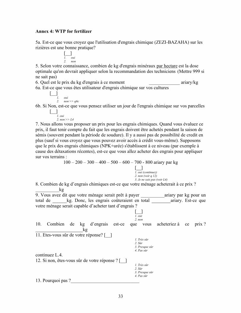
33

Annex 4: WTP for fertilizer 5a. Est-ce que vous croyez que l'utilisation d'engrais chimique (ZEZI-BAZAHA) sur les rizières est une bonne pratique? [__]

1. oui 2. non

5. Selon votre connaissance, combien de kg d'engrais minéraux par hectare est la dose optimale qu'on devrait appliquer selon la recommandation des techniciens (Mettre 999 si ne sait pas) 6. Quel est le prix du kg d'engrais à ce moment _____________ ariary/kg 6a. Est-ce que vous êtes utilisateur d'engrais chimique sur vos cultures [__]

1. oui 2. non >> q6c

6b. Si Non, est-ce que vous pensez utiliser un jour de l'engrais chimique sur vos parcelles [__]

1. oui 2. non >> L4

7. Nous allons vous proposer un prix pour les engrais chimiques. Quand vous évaluez ce prix, il faut tenir compte du fait que les engrais doivent être achetés pendant la saison de sémis (souvent pendant la période de soudure). Il y a aussi pas de possibilité de credit en plus (sauf si vous croyez que vous pouvez avoir accès à crédit vous-même). Supposons que le prix des engrais chimiques (NPK+urée) s'établissent à ce niveau (par exemple à cause des détaxations récentes), est-ce que vous allez acheter des engrais pour appliquer sur vos terrains :

100 – 200 – 300 – 400 – 500 – 600 – 700 - 800 ariary par kg [__] 1. oui (continuez) 2. non (voir q 12) 3. Je ne sais pas (voir L4)

8. Combien de kg d’engrais chimiques est-ce que votre ménage acheterait à ce prix ? __________kg 9. Vous avez dit que votre ménage serait prêt à payer __________ariary par kg pour un total de ______kg. Donc, les engrais coûteraient en total ________ariary. Est-ce que votre ménage serait capable d’acheter tant d’engrais ?

[__] 1. oui 2. non

10. Combien de kg d’engrais est-ce que vous acheteriez à ce prix ? ____________________kg 11. Etes-vous sûr de votre réponse? [__]

1. Très sûr 2. Sûr 3. Presque sûr 4. Pas sûr

continuez L.4. 12. Si non, êtes-vous sûr de votre réponse ? [__]

1. Très sûr 2. Sûr 3. Presque sûr 4. Pas sûr

13. Pourquoi pas ?_____________________________

Table 1: Farm characteristics by income level

Income quintile in 2002

Mean St.Dev. Mean St.Dev. Mean St.Dev. Mean St.Dev. Mean St.Dev. Mean St.Dev.Income - welfare measuresPer capita annual income ariary 2002 28,680 10,001 54,695 6,428 86,552 10,610 128,144 19,722 334,275 306,853 116,724 165,111Per capita agri. income ariary 2002 20,212 9,758 36,199 14,079 54,984 22,561 77,234 31,373 155,645 96,184 64,337 63,609Length of lean season month 2002 5.95 2.52 5.42 2.50 5.66 2.40 4.58 2.76 3.88 2.86 5.18 2.69Rice productionTotal rice production kg 2002 501.85 390.59 723.56 527.25 955.88 758.65 1,362.81 1,361.74 1,671.93 1,803.74 998.26 1,128.67

2003 704.88 492.41 871.31 598.35 924.25 658.36 1,424.64 1,463.95 1,698.67 1,696.07 1,086.34 1,108.21Total cultivated rice area ares 2002 39.46 27.97 37.35 37.15 50.83 43.47 59.10 62.13 72.26 75.38 48.20 52.29

2003 31.13 31.48 38.74 39.83 50.44 42.90 59.45 61.92 72.07 75.62 48.83 52.87Household characteristics and assetsTotal agricultural land area ares 2002 76.49 80.95 82.50 79.99 135.18 107.53 160.28 156.97 161.76 143.92 119.68 119.31

2003 79.02 82.82 83.93 72.74 134.03 106.58 160.62 156.90 161.57 142.43 120.37 119.01Family size no 2002 8.06 2.65 8.14 4.19 7.04 2.88 6.71 3.23 4.86 2.38 7.07 3.31

2003 8.54 2.83 8.49 4.58 7.27 3.01 7.05 3.52 5.07 2.49 7.40 3.56Number of adults/hh no 2002 3.74 2.02 3.75 2.60 3.43 1.71 3.35 1.77 2.75 1.46 3.44 1.98

2003 3.81 2.08 3.77 2.61 3.48 1.77 3.39 1.84 2.79 1.52 3.48 2.03Value of agricultural equipmentsAriary 2002 8,568 27,054 47,916 109,001 27,761 67,720 58,760 108,427 85,990 125,487 42,896 94,556

2003 11,258 32,566 49,301 108,864 29,132 69,100 59,957 109,567 86,943 126,625 44,484 95,479Owner of weeder 1=own 2002 0.08 0.32 0.20 0.44 0.23 0.61 0.25 0.55 0.36 0.62 0.21 0.52

2003 0.09 0.38 0.21 0.45 0.23 0.61 0.27 0.62 0.42 0.72 0.23 0.56Number of cattle & cows no 2002 1.78 2.13 2.09 2.42 1.54 1.95 2.33 2.34 2.98 3.46 2.10 2.50

2003 1.64 2.17 2.31 3.46 1.53 1.74 2.17 2.32 2.90 2.93 2.07 2.60Characteristics of household chiefGender 1=male 2002 0.85 0.35 0.93 0.25 0.95 0.21 0.95 0.23 0.89 0.32 0.91 0.28Age in 2002 years 2002 31.07 27.21 32.78 20.98 36.10 23.53 35.82 24.56 39.43 24.29 34.90 24.28Education level 0 to 6 2002 2.12 0.66 2.50 0.76 2.41 0.80 2.33 0.69 2.66 1.00 2.39 0.80Number of observations 151 149 148 150 148 746Source: BASIS CRSP 2002, 2003 surveys

Quintile 5 OverallQuintile 1 Quintile 2 Quintile 3 Quintile 4

Table 2: Access and use of production factors in rice by income level

Income quintile 2002

Mean St.Dev. Mean St.Dev. Mean St.Dev. Mean St.Dev. Mean St.Dev. Mean St.Dev.Average return to labor Ariary/day 2002 1456 2408 2425 3054 3370 2457

Average rice yield kg/are 2002 21.3 16.9 26.7 17.3 23.5 16.6 29.6 18.5 28.9 21.9 26.4 18.92003 25.8 18.4 26.8 16.4 23.9 17.2 28.2 17.9 31.4 19.8 27.5 18.3

Average plot size ares 2002 11.1 13.1 10.9 10.8 16.7 18.1 16.2 19.9 20.5 22.5 15.1 17.72003 12.6 13.1 13.1 12.3 15.8 15.8 18.8 24.0 19.3 20.5 15.9 17.9

Total Labor hours/are 2002 23.4 12.4 17.7 10.2 15.5 9.6 15.5 10.1 13.7 9.7 17.2 10.92003 19.0 11.9 15.5 8.9 13.5 9.1 14.8 10.1 11.6 7.1 14.9 9.9

Transplanting labor hours/are 2002 3.43 4.31 3.74 3.46 2.88 3.90 3.98 5.67 3.45 2.85 3.50 4.162003 2.71 2.49 3.27 3.04 2.41 2.11 3.00 2.68 3.36 2.61 2.95 2.62

Age of transplanted plants days 2002 49.25 17.82 49.02 16.92 48.40 14.95 44.20 16.32 38.26 16.55 45.85 17.022003 44.92 14.13 13.93 12.22 42.63 10.51 40.82 12.63 42.02 13.34 42.87 12.68

Technique of transplanting 1= in line 2002 0.54 0.57 0.46 0.50 0.48 0.50 0.56 0.54 0.39 0.63 0.49 0.552003 0.53 0.50 0.46 0.50 0.48 0.54 0.54 0.58 0.42 0.50 0.49 0.52

Weeding labor hours/are 2002 5.01 8.25 4.85 6.78 3.00 3.05 4.21 5.48 3.58 3.97 4.14 5.862003 3.11 3.13 3.40 3.09 2.17 2.06 3.08 2.73 3.20 5.22 2.99 3.44

Mineral fertilizer users 1=user 2002 0.24 0.42 0.36 0.48 0.32 0.47 0.25 0.43 0.28 0.45 0.29 0.462003 0.23 0.42 0.36 0.48 0.22 0.42 0.25 0.44 0.41 0.49 0.30 0.46

Selected seeds users 1=user 2002 0.55 0.50 0.43 0.50 0.57 0.49 0.48 0.50 0.40 0.49 0.49 0.502003 0.52 0.50 0.46 0.50 0.50 0.50 0.39 0.49 0.38 0.49 0.45 0.50

Drought 1=yes 2002 0.14 0.35 0.15 0.36 0.18 0.39 0.14 0.35 0.12 0.33 0.15 0.352003 0.15 0.36 0.13 0.33 0.13 0.34 0.12 0.33 0.11 0.31 0.13 0.33

Flooding 1=yes 2002 0.13 0.33 0.13 0.33 0.11 0.32 0.07 0.26 0.10 0.30 0.11 0.312003 0.07 0.25 0.07 0.26 0.07 0.26 0.07 0.26 0.11 0.31 0.08 0.27

Number of observations 151 149 148 150 148 746Source: BASIS CRSP 2002, 2003 surveys; Numbers in italics are standard deviation

Quintile 5 OverallQuintile 1 Quintile 2 Quintile 3 Quintile 4

Table 3: Self-proclaimed constraints to improved agricultural productivity as stated by agricultural households

Rank* Percentage of households that

Variables not a bit quite very totalConstraints to overall agricultural productivityEPM 2001, 2470 agricultural householdsAccess to agricultural equipment 1 19 18 27 35 100Access to land 2 27 19 29 25 100Access to cattle for labor 3 24 23 29 24 100Access to labor 4 22 28 30 20 100Access to credit 5 36 19 23 22 100Degradation of irrigation infrastructure due to environmental problems6 29 31 22 18 100Access to agricultural inputs (as fertilizer) 7 34 26 19 21 100Access to cattle for fertilizer 8 42 23 19 16 100Land tenure insecurity 9 44 26 22 8 100Silting of land 10 46 29 18 7 100EPM 2004, 3543 agricultural householdsAccess to agricultural equipment 1 11 14 32 43 100Access to irrigation 2 13 21 29 37 100Access to cattle for labor 3 16 20 35 29 100Access to labor 4 17 22 37 24 100Avoid droughts 4 20 19 27 34 100Access to agricultural inputs (as fertilizer) 6 24 20 26 30 100Phyto-sanitary diseases 7 19 25 30 26 100Avoid flooding 8 25 20 26 29 100Access to cattle for fertilizer 9 28 22 25 25 100Access to credit 10 31 23 22 24 100Silting of land 11 33 29 23 15 100Land tenure insecurity 12 38 24 23 15 100Constraints to rice productivityCommune survey 2004, 290 communal focus groupsAccess to better irrigation systems 1 3 12 27 58 100Access to agricultural equipment 2 4 19 27 50 100Access to livestock to work the land 3 8 22 27 43 100Access to credit 4 16 24 23 37 100Avoid losses due to plant diseases 5 11 31 24 34 100Avoid floods 6 16 26 22 36 100Access to improved seeds 7 13 29 21 37 100Access to labor 8 17 27 26 30 100Access to chemical fertilizer 9 29 29 20 22 100Access to livestock for manure 10 26 32 20 22 100Avoid silting 11 22 36 21 21 100Avoid droughts 12 48 15 12 25 100Land tenure 13 27 37 23 13 100

Access to cattle for manure 1 5 6 13 76 100Access to better irrigation 2 5 14 20 61 100Access to credit 3 11 8 37 44 100Access to agricultural inputs (fertilizer) 4 4 17 35 44 100Access to labor 5 10 15 40 35 100Access to agricultural equipment 6 20 15 26 39 100Access to cattle for labor 7 28 11 25 36 100Avoid losses due to plant diseases 8 19 23 42 16 100Avoid droughts 9 22 23 27 28 100Avoid floods 10 24 37 25 14 100Insecure property rights 11 59 11 14 16 100Avoid silt 12 34 38 21 7 100

state this constraint is … important

Basis Crsp survey, 2003, 316 agricultural household in highlands

* based on the 'important' and 'very important' category

Table 4: Results of normalized quadratic production function - household panel data analysis

Dependent variable = Yield in kg/are Coefficient t-value Coefficient t-value

b1 Total cultivated land in ares -0.074 -0.770 -0.087 -0.890b2 Predicted labor use in hours/are 1.275 10.430 2.227 9.880b3 Total Value of Agricultural Equipment in Ariary -0.018 -0.930 -0.023 -1.200b4 Number of zebu, draught oxen -0.170 -0.280 -0.031 -0.050b5 Chemical fertilizer in kg/are 1.135 0.800 0.397 0.290b6 Age at transplantation in days -0.104 -2.040 -0.115 -2.260b7 Climatic idiosynchratic risks -12.801 -4.240 -11.695 -3.850b1b1 B1 squared 0.000 1.370 0.000 1.290b1b2 Interaction b1 and b2 0.000 0.150 -0.002 -0.760b1b3 Interaction b1 and b3 0.000 -0.300 0.000 0.140b1b4 Interaction b1 and b4 0.005 1.690 0.006 1.830b1b5 Interaction b1 and b5 0.003 0.310 0.008 0.900b1b6 Interaction b1 and b6 0.000 0.960 0.001 1.630b1b7 Interaction b1 and b7 0.037 1.350 0.032 1.180b2b2 B2 squared -0.027 -4.180 -0.056 -4.550b2b3 Interaction b2 and b3 0.002 1.540 0.004 2.330b2b4 Interaction b2 and b4 0.041 1.170 0.098 2.010b2b5 Interaction b2 and b5 0.012 0.160 0.137 1.210b2b6 Interaction b2 and b6 -0.003 -0.800 -0.004 -0.700b2b7 Interaction b2 and b7 -0.319 -1.300 -0.473 -1.360b3b3 B3 squared 0.000 0.340 0.000 1.330b3b4 Interaction b3 and b4 0.000 -0.150 0.001 0.280b3b5 Interaction b3 and b5 0.007 0.800 0.002 0.280b3b6 Interaction b3 and b6 -0.001 -1.800 0.000 0.120b3b7 Interaction b3 and b7 0.030 1.350 0.030 1.310b4b4 B4 squared 0.070 1.290 0.079 1.440b4b5 Interaction b4 and b5 -0.154 -0.560 -0.326 -1.180b4b6 Interaction b4 and b6 -0.009 -0.480 -0.028 -1.450b4b7 Interaction b4 and b7 0.603 0.750 0.726 0.900b5b5 B5 squared -0.100 -2.100 -0.178 -2.580b5b6 Interaction b5 and b6 0.077 2.610 0.081 2.750b5b7 Interaction b5 and b7 -7.209 -0.950 -10.593 -1.390b6b6 B6 squared 0.001 0.930 0.000 -0.160b6b7 Interaction b6 and b7 0.131 0.920 0.184 1.270Intercept 49.190 4.830 40.626 3.580Number of observations 1500 1500F 6.080 5.830Prob>F 0.000 0.000R-squared within 0.222 0.215

between 0.178 0.179overall 0.177 0.175

Source: BASIS CRSP 2002, 2003 surveys

Regular Instrumented

Table 5: Marginal physical returns and shift in productivity of factor of production - household panel data analysis

Income quintile in 2002Quintile 1 Quintile 2 Quintile 3 Quintile 4 Quintile 5 Overall Sign of F-test

InstrumentedTotal cultivated area Additional kg of paddy per are -0.02 -0.01 0.00 0.02 0.04 0.01

Doubling area: Yield increases by -5.1% -1.9% 1.1% 7.0% 20.9% 4.3%Labor kg of paddy per hour 1.05 1.38 1.25 1.33 1.65 1.33 ***

Doubling labor: Yield increases by 53.3% 56.7% 48.2% 47.5% 46.7% 50.5%Value of agricultural equipment Kg of paddy per hour 0.06 0.05 0.04 0.04 0.04 0.04

Doubling traction: Yield increases by 1.1% 3.3% 2.2% 3.4% 4.7% 2.9%Number of zebu, draught oxen, cows kg of paddy per kg of fertilizer 1.04 0.93 0.97 1.27 1.38 1.12 **

Doubling fertilizer: Yield increases by 5.3% 7.1% 4.7% 7.5% 12.5% 7.4%Chemical fertilizer Kg of paddy per kg of fertilizer 5.75 5.03 5.50 5.59 4.49 5.27 ***

Doubling manure: Yield increase by 7.8% 4.5% 1.4% 2.1% 4.9% 4.2%Age of plants (technology) kg of paddy per day -0.14 -0.15 -0.10 -0.09 -0.07 -0.11 **

Doubling age: Yield decrease -12.8% -18.6% -12.9% -10.1% -6.2% -13.0%Climatic shocks Yield changes in kg/are if shocks -13.18 -8.05 -4.53 -4.03 -4.16 -6.81 ***

% change on yield if shocksNon-instrumentedTotal cultivated area Additional kg of paddy per are 0.02 0.03 0.04 0.05 0.07 0.04Labor kg of paddy per hour 0.65 0.84 0.85 0.89 1.06 0.86 ***Value of agricultural equipment Kg of paddy per hour -0.01 -0.02 -0.02 -0.02 -0.02 -0.02Number of zebu, draught oxen, cows kg of paddy per kg of fertilizer 0.75 0.72 0.79 1.01 1.16 0.89Chemical fertilizer Kg of paddy per kg of fertilizer 4.23 4.12 4.31 4.29 3.74 4.14 ***Age of plants (technology) kg of paddy per day -0.02 -0.03 0.00 0.00 0.03 0.00 **Climatic shocks Yield changes in kg/are if shocks -12.94 -8.66 -5.99 -5.2 -4.27 -7.43 ***F-test is used to check the significance for each variable. If tests jointly, at least one of the coefficient estimates

differs from zero; ***, * indicate significance level at the 1% and 10% levelSource: BASIS CRSP 2002, 2003 surveys

Table 6: Determinants of rice yields (OLS) - spatial data analysis

Dependent variable = log of average rice yield in communeVariable Unit Coeff. t-value#% of hhs that adopt land intensification improved technology* 0 to 5 0.0368 2.569% of lowlands connected to improved irrigation infrastructure % 0.0013 3.669% of hhs that adopt agr. equipment 0 to 5 0.0198 2.225% of hhs that adopt off-season crops 0 to 5 0.0005 0.071log(# of years in last three when hit by major disasters) 0 to 27 -0.0081 -0.495log ((number of cattle+1)/(population in commune)) # 0.0284 3.909use of animal traction (% of farmers) % 0.0010 2.727population density log(no) -0.0057 -0.570% of population that belongs to cattle/rice cultivators ethnic group % 0.0011 2.387% of population that belongs to the forest ethnic group % -0.0014 -2.196% of population that belongs to eastern ethnic group % 0.0012 2.293% of population that belongs to western ethnic group % 0.0005 0.645average temperature in the commune C -0.0249 -1.397average temperature in the commune squared 0.0000 1.050average rainfall in the commune mm 0.0002 1.098average rainfall in the commune squared 0.0000 -1.047average altitude in the commune m -0.0001 -0.226average altitude in the commune squared 0.0000 -0.939% of the surface commune with cristalline soils - North/Highlands % -0.0002 -0.259% of the surface commune with cristalline soils - Midwest % -0.0002 -0.271% of the surface commune with cristalline soils - East % -0.0001 -0.090% of the surface commune with cristalline soils - South % -0.0020 -3.139% of the surface commune with volcanic soils % -0.0004 -0.635% of the surface commune with alluvial soils % -0.0002 -0.354Dummy province of Fianarantsoa 1=yes -0.1420 -3.899Dummy province of Toamasina 1=yes -0.0522 -1.035Dummy province of Mahajanga 1=yes -0.0610 -0.979Dummy province of Toliara 1=yes -0.1033 -1.556Dummy province of Antsiranana 1=yes -0.1706 -2.199Intercept 10.6338 5.671Number of observations 1272F(29,1242) 22.69Prob > F 0.00R-squared 0.32Root MSE 0.34Exogeneity and endogeneity testsA. yield regressions Test p-valuea. Davidson McKinnon endogeneity test Adoption t-value 1.06 0.29b. Overidentification testsTest that istruments are exogenousWald Χ2 15.13 0.00B. Instrumenting regressionsTest that instruments are jointly significant**F-test F-value 12.60 0.00# standard errors and t-values corrected for spatial autocorrelation* endogenous in 2SLS (instruments: pop. density, remoteness, distance ag. Extension, sceurity, titled land)

Table 7: Determinants of adoption of improved agricultural technologies (ordered probit) - spatial data analysis

Variable Unit coefficient z-value coefficient z-value coefficient z-value coefficient z-value% of lowlands connected to improved irrigation infrastructure % 0.002 1.210 0.004 3.030 0.005 2.950 0.004 3.130perceived security conditions 1 to 5 0.010 0.250 0.023 0.560 -0.156 -3.540 -0.071 -1.750population density log(number) -0.010 -0.250 0.038 0.910 -0.114 -2.270 0.021 0.490remoteness quintile -0.123 -3.280 -0.204 -5.230 -0.138 -3.280 -0.091 -2.420% of population that belongs to cattle/rice cultivators ethnic group % -0.009 -4.980 -0.005 -2.380 -0.008 -3.510 -0.006 -3.290% of population that belongs to the forest ethnic group % -0.007 -3.300 -0.011 -4.180 -0.002 -0.800 -0.002 -0.860% of population that belongs to eastern ethnic group % -0.001 -0.570 -0.004 -1.910 0.002 0.740 -0.004 -1.840% of population that belongs to western ethnic group % -0.011 -3.800 -0.005 -1.620 -0.020 -5.730 -0.007 -2.270distance to extension agent log(distance) -0.023 -1.010 -0.034 -1.400 -0.054 -2.040 -0.034 -1.490% of agricultural land that is titled % -0.047 -1.560 0.015 0.430 0.016 0.380 0.117 3.910% of adults in the commune that are literate % 0.006 1.930 0.008 2.670 0.005 1.500 0.007 2.100log(# of years in last three when hit by major disasters) 0 to 27 0.175 2.960 0.047 0.710 0.220 3.060 0.096 1.550average temperature in the commune C -0.156 -2.700 -0.294 -4.530 0.223 3.080 0.004 0.070average temperature in the commune squared 0.000 2.440 0.001 4.560 0.000 -2.460 0.000 1.060average rainfall in the commune mm 0.001 1.730 0.000 -0.350 0.003 4.710 0.000 0.240average rainfall in the commune squared 0.000 -0.920 0.000 0.380 0.000 -3.860 0.000 0.220average altitude in the commune m 0.001 0.740 0.002 2.200 0.001 1.600 0.005 5.970average altitude in the commune squared 0.000 -0.960 0.000 -3.250 0.000 2.630 0.000 -2.550% of the surface commune with cristalline soils - North/Highlands % 0.000 -0.110 0.003 1.220 0.002 0.910 0.003 1.120% of the surface commune with cristalline soils - Midwest % 0.000 -0.120 0.004 1.340 -0.004 -0.800 0.001 0.390% of the surface commune with cristalline soils - East % 0.001 0.250 0.002 0.700 0.002 0.930 0.002 0.780% of the surface commune with cristalline soils - South % 0.008 2.940 0.000 0.010 0.020 5.680 0.007 2.900% of the surface commune with volcanic soils % -0.001 -0.390 0.004 1.350 0.001 0.340 0.004 1.680% of the surface commune with alluvial soils % -0.003 -1.030 0.003 1.160 0.005 1.690 0.008 3.210Dummy province of Fianarantsoa 1=yes -0.112 -1.080 -0.013 -0.110 1.228 4.810 0.375 3.250Dummy province of Toamasina 1=yes 0.367 1.890 0.384 1.620 -0.816 -3.050 0.735 4.050Dummy province of Mahajanga 1=yes 1.097 4.630 -0.565 -2.090 -0.046 -0.150 0.166 0.640Dummy province of Toliara 1=yes 1.337 5.400 0.563 2.230 1.358 3.790 1.135 4.510Dummy province of Antsiranana 1=yes 1.681 6.780 -0.317 -1.060 -1.261 -3.840 0.192 0.680Number of observations 1342 1342 1342 1350Wald Χ2 622.58 639.92 460.06 331.29 p-value (Prob>Χ2) 0 0 0 0Pseudo R2 0.1767 0.2341 0.2254 0.0943

off-season crops fertilizer early transplanting improved seeds

Table 7: Determinants of adoption of improved agricultural technologies (ordered probit) - continued

Variable Unit coefficient z-value coefficient z-value coefficient z-value% of lowlands connected to improved irrigation infrastructure % 0.006 3.830 0.002 1.280 0.006 4.720perceived security conditions 1 to 5 -0.052 -1.150 0.008 0.210 -0.099 -2.780population density log(number) -0.028 -0.620 -0.084 -2.010 0.002 0.040remoteness quintile -0.130 -3.000 -0.170 -4.540 -0.170 -4.640% of population that belongs to cattle/rice cultivators ethnic group % 0.000 -0.060 -0.002 -1.090 -0.004 -2.480% of population that belongs to the forest ethnic group % 0.000 0.070 -0.014 -4.870 -0.003 -1.820% of population that belongs to eastern ethnic group % 0.000 -0.130 -0.009 -4.660 -0.003 -2.000% of population that belongs to western ethnic group % 0.001 0.180 0.003 1.040 -0.011 -3.730distance to extension agent log(distance) -0.097 -3.780 -0.009 -0.400 -0.054 -2.410% of agricultural land that is titled % 0.083 2.450 -0.012 -0.390 0.085 2.370% of adults in the commune that are literate % 0.011 3.440 0.017 5.530 0.007 2.460log(# of years in last three when hit by major disasters) 0 to 27 0.118 1.650 0.247 3.830 0.149 2.640average temperature in the commune C 0.002 0.030 0.228 3.460 -0.024 -0.460average temperature in the commune squared 0.000 0.530 0.000 -3.190 0.000 1.400average rainfall in the commune mm -0.001 -0.850 0.003 4.490 0.001 2.400average rainfall in the commune squared 0.000 1.020 0.000 -4.670 0.000 -1.830average altitude in the commune m 0.002 2.360 0.001 1.460 0.003 4.670average altitude in the commune squared 0.000 -0.190 0.000 1.250 0.000 -1.000% of the surface commune with cristalline soils - North/Highlands % 0.004 1.470 0.003 1.530 0.003 1.250% of the surface commune with cristalline soils - Midwest % 0.002 0.420 0.008 1.790 -0.001 -0.150% of the surface commune with cristalline soils - East % 0.009 3.000 -0.005 -2.310 0.002 1.040% of the surface commune with cristalline soils - South % 0.005 1.380 0.007 3.370 0.008 3.670% of the surface commune with volcanic soils % 0.003 0.750 0.003 1.290 0.003 1.180% of the surface commune with alluvial soils % 0.004 1.370 0.002 0.680 0.006 2.730Dummy province of Fianarantsoa 1=yes -0.094 -0.810 -0.532 -4.220 0.308 2.570Dummy province of Toamasina 1=yes -0.255 -1.240 -0.002 -0.010 -0.302 -1.640Dummy province of Mahajanga 1=yes -0.513 -2.030 0.095 0.380 -0.501 -2.430Dummy province of Toliara 1=yes -0.314 -1.120 0.817 3.340 0.720 3.460Dummy province of Antsiranana 1=yes -0.562 -1.890 -0.098 -0.340 -0.990 -3.950Number of observations 1342 1342 1342Wald Χ2 439.44 741.92 554.2 p-value (Prob>Χ2) 0 0 0Pseudo R2 0.2075 0.26 0.1814* adoption index = mean of adoption of land intensification technologies, i.e. fertilizer, transplanting, improved seeds, sri

sri agr. equipment adoption index*

Table 8: Determinants for the willingness-to-pay for fertilizer - logit

Variable* Unit Mean St. Dev. Coefficient z-value Coefficient z-valueAccept the bid yes=1 0.652Log(bid level) Ariary 5.922 0.668 -2.866 -5.330 -5.537 -4.750 household characteristics Age of the head of household number 47.644 12.790 -0.050 -2.550Highest education level in the household 1 to 6 2.831 0.844 -0.120 -0.400Gender of the head of household male=1 0.905 0.294 0.945 0.950Total income log(Ariary) 13.099 0.796 0.143 0.390Events over the last ten years**Number of years of flooding number 1.019 2.372 -0.046 -0.470Number of years of drought number 1.090 2.052 -0.021 -0.190Number of years of late planting number 1.134 1.571 -0.056 -0.310Number of years of off-season crops number 2.891 3.185 0.214 2.920Beliefs and constraints on agricultureThinks fertilizer is beneficial for ricefields yes=1 0.678 0.468 1.795 1.920Importance of constraints (1=not;2=a bit;3=quite;4=very)Insecure property rights 1 to 4 1.858 1.160 -0.291 -1.190Access to cattle for labor 1 to 4 2.695 1.222 0.148 0.380Access to cattle for manure 1 to 4 3.604 0.812 -0.001 0.000Access to labor 1 to 4 3.006 0.949 -0.100 -0.180Access to agricultural equipment 1 to 4 2.842 1.146 -0.041 -0.110Access to agricultural inputs (fertilizer) 1 to 4 3.209 0.843 -0.443 -1.150Access to better irrigation 1 to 4 3.383 0.892 -0.106 -0.380Access to credit 1 to 4 3.142 0.977 0.736 1.260Number of observations 284 220Wald chi2 44.73 62.19Prob>chi2 0.0002 0.0011Pseudo R2 0.3341 0.5435Source: Authors' calculations based on the Basis Crsp 2003 survey *: village dummies included but not reported**: data only for one particular rice plot; used as proxy for all plots

Parsimonious model Comprehensive model

Table 9: Determinants of the willingness to contribute to a water user association - logit

Variable* Unit Mean St. Dev. Coefficient z-value Coefficient z-valueAccept the bid yes=1 0.539Log(bid level) Ariary 4.592 1.431 -0.909 -7.850 -1.223 -6.560Plot characteristicsPlot area log(ares) 2.466 0.953 -0.585 -2.240Difference between highest and lowest production in last 10 year log(no) 5.343 0.879 0.556 2.430household characteristicsAge of the head of household number 47.644 12.790 -0.020 -1.340Highest education level in the household 1 to 6 2.831 0.844 0.060 0.230Gender of the head of household male=1 0.905 0.294 0.192 0.220Total income log(Ariary) 13.099 0.796 0.545 1.830Events over the last ten yearsNumber of years of flooding number 1.019 2.372 -0.039 -0.500Number of years of drought number 1.090 2.052 0.096 0.860Number of years of late planting number 1.134 1.571 0.337 2.100Number of years of off-season crops number 2.891 3.185 -0.063 -0.940Constraints on agricultureImportance of constraints (1=not;2=a bit;3=quite;4=very)Insecure property rights 1 to 4 1.858 1.160 -0.017 -0.080Access to cattle for labor 1 to 4 2.695 1.222 0.154 0.540Access to cattle for manure 1 to 4 3.604 0.812 0.142 0.530Access to labor 1 to 4 3.006 0.949 -0.049 -0.200Access to agricultural equipment 1 to 4 2.842 1.146 0.231 0.840Access to agricultural inputs (fertilizer) 1 to 4 3.209 0.843 0.080 0.330Access to better irrigation 1 to 4 3.383 0.892 0.853 3.380Access to credit 1 to 4 3.142 0.977 -0.386 -1.540Number of observations 313 255Wald chi2 74.2 90.65Prob>chi2 0 0Pseudo R2 0.2415 0.4033Source: Authors' calculations based on the Basis Crsp 2003 survey*: village dummies included but not reported

Parsimonious model Comprehensive model

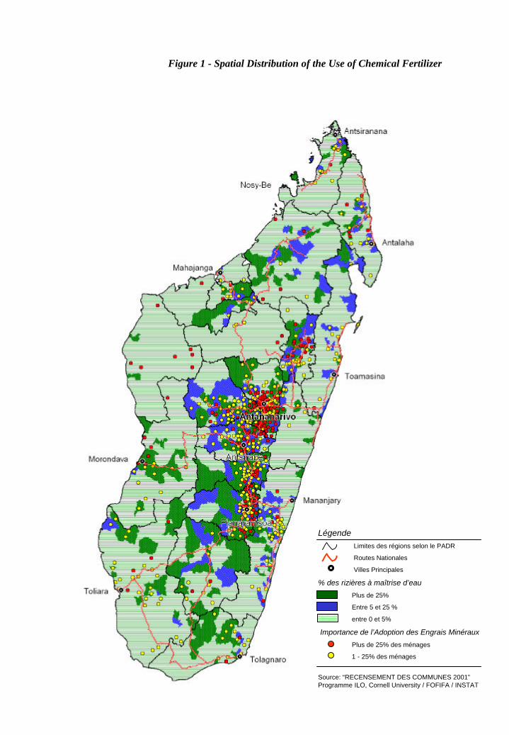
Figure 1 - Spatial Distribution of the Use of Chemical Fertilizer

LégendeLimites des régions selon le PADR

Routes Nationales

Villes Principales

% des rizières à maîtrise d’eau

Plus de 25%

Entre 5 et 25 %

entre 0 et 5%

Importance de l’Adoption des Engrais Minéraux

Plus de 25% des ménages

1 - 25% des ménages

Source: “RECENSEMENT DES COMMUNES 2001”Programme ILO, Cornell University / FOFIFA / INSTAT

Figure 2 - Spatial Distribution of the Adoption of New Rice Variety

LégendeLimites des régions selon le PADR

Routes Nationales

Villes Principales

Certaines Variétés dominantes dans les communes

Makalioka

Rojo

Tsipala

Diffusion des certaines "nouvelles" variétés

Variétés IR8, IR16, IR20, IR36, etc…

Variétés X265, X360, etc…

Source: “RECENSEMENT DES COMMUNES 2001”Programme ILO, Cornell University / FOFIFA / INSTAT

Figure 3 - Spatial Distribution of the Main Crop by Cultivated Area

LégendeLimites des régions selon le PADR

Routes Nationales

Villes Principales

Principale Culture dans la commune (Surface)

Riz

Autres Cultures: Manioc, Maïs, Arachide …

Cultures Industrielles: Coton, Canne …

Cultures d'exportation: vanille, Café …

Pas de données

Source: “RECENSEMENT DES COMMUNES 2001”Programme ILO, Cornell University / FOFIFA / INSTAT

Figure 4 - Spatial Distribution of the Adoption of SRI

LégendeLimites des régions selon le PADR

Routes Nationales

Villes Principales

% des rizières à maîtrise d’eau

Plus de 25%

Entre 5 et 25 %

entre 0 et 5%

Importance de l’Adoption du SRI

Plus de 25% des ménages

1 - 25% des ménages

Source: “RECENSEMENT DES COMMUNES 2001”Programme ILO, Cornell University / FOFIFA / INSTAT

Figure 5 - Spatial Distribution of the practice of Contre-Saison

LégendeLimites des régions selon le PADR

Routes Nationales

Villes Principales

% des rizières à maîtrise d’eau

Plus de 25%

Entre 5 et 25 %

entre 0 et 5%

Importance de la pratique de Contre-Saison

Plus de 25% des ménages

1 - 25% des ménages

Source: “RECENSEMENT DES COMMUNES 2001”Programme ILO, Cornell University / FOFIFA / INSTAT

Harvest 2000Harvest 2001Harvest 2002Harvest 2003Harvest 2004NPK 600 500 1200 550 1000Paddy 230 120 170 190 260

Harvest 2000Harvest 2001Harvest 2002Harvest 2003Harvest 2004Ratio price paddy over price NPK2.6 4.2 7.1 2.9 3.8Ratio value output over cost fertilizer2.6 1.7 1.0 2.4 1.8

Figure 6: Cost - benefit ratios for chemical fertilizer and paddy

0.0

1.0

2.0

3.0

4.0

5.0

6.0

7.0

8.0

Harvest 2000 Harvest 2001 Harvest 2002 Harvest 2003 Harvest 2004

Rat

io

Ratio price paddy over price NPK

Ratio value output over costfertilizer

100 0.923077 39200 0.923077 39300 0.916667 36400 0.828571 35500 0.540541 37600 0.552632 38700 0.297297 37800 0.236842 38

Figure 7: Demand for chemical fertilizer by price level

0

0.1

0.2

0.3

0.4

0.5

0.6

0.7

0.8

0.9

1

100 200 300 400 500 600 700 800Ariary/kg

Pro

porti

on o

f far

mer

s th

at u

se fe

rtiliz

er

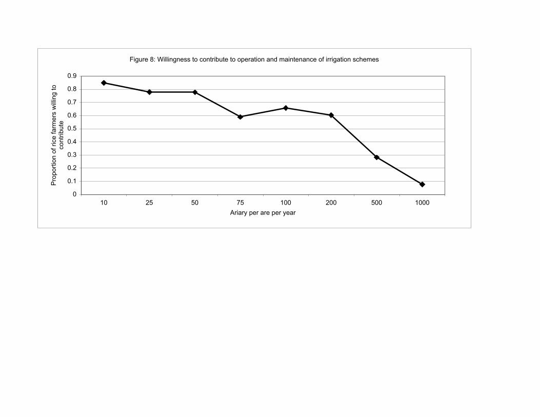
10 0.85 4025 0.780488 4050 0.777778 3675 0.589744 39

100 0.658537 41200 0.605263 37500 0.282051 38

1000 0.076923 39

Figure 8: Willingness to contribute to operation and maintenance of irrigation schemes

0

0.1

0.2

0.3

0.4

0.5

0.6

0.7

0.8

0.9

10 25 50 75 100 200 500 1000Ariary per are per year

Pro

porti

on o

f ric

e fa

rmer

s w

illin

g to

co

ntrib

ute

Figure 9: Willingness to contribute to operation and maintenance of irrigation infrastructure (simulations based on regression results)

0

0.1

0.2

0.3

0.4

0.5

0.6

0.7

0.8

0.9

1

10 25 50 75 100 200 500 1000Ariary per year per are

Pro

porti

on o

f ric

e fa

rmer

s w

illin

g to

co

ntrib

ute

Income quintile 1Income quintile 2Income quintile 3Income quintile 4Income quintile 5