getting started with hysys oli

Page i

Getting Started with Hysys™ OLI™

OLI Systems, Inc.

Version 3.2

Page ii

©Copyright 2006 OLI Systems, Inc. All rights reserved. The enclosed materials are provided to the lessees, selected individuals and agents of OLI Systems, Inc. The material may not be duplicated or otherwise provided to any entity with out the expressed permission of OLI Systems, Inc.

108 American Road

Morris Plains, New Jersey 07950 973-539-4996

(Fax) 973-539-5922 [email protected]

www.olisystems.com

Hysys is the trademark of Aspen Technologies Inc. Cambridge, MA OLI is the trademark of OLI Systems, Inc. Morris Plains, NJ

Contents Contents .......................................................................................................................... 3

Chapter 1 Introduction to OLI Electrolytes ........................................................................ 4 Overview......................................................................................................................... 4 Understanding Aqueous Electrolyte Systems................................................................. 5 Aqueous Electrolytes Primer ........................................................................................ 11 The OLI Thermodynamic Framework.......................................................................... 13

Other Physical Phases in Equilibrium With the Aqueous Phase .............................. 14 What OLI Provides ....................................................................................................... 15 Range of Applicability of the OLI Model..................................................................... 15

The OLI Databank .................................................................................................... 17 The OLI Engine ........................................................................................................ 18

Chapter 2 Getting Started with Hysys OLI....................................................................... 19 Introduction................................................................................................................... 19 Assumptions.................................................................................................................. 19 Starting HYSYS OLI (HEO) ........................................................................................ 19

Starting a new case.................................................................................................... 19 Entering the Simulation Environment. ..................................................................... 24

Chapter 3 Aqueous Thermodynamics............................................................................... 27 Overview....................................................................................................................... 27 The Equilibrium Constant............................................................................................. 27

Question: ................................................................................................................... 28 Principal Thermodynamic Properties ........................................................................... 29 HKF (Helgeson-Kirkham-Flowers)Equation of State,.................................................. 29

The Helgeson Equation of State ............................................................................... 32 What is the standard State? ....................................................................................... 33

Excess Properties .......................................................................................................... 34 Ionic Strength............................................................................................................ 34 Definition of Aqueous Activity Coefficients............................................................ 35 Long Range Terms.................................................................................................... 37 Short Range Terms ................................................................................................... 38 Modern Formulations................................................................................................ 39 Neutral Species ......................................................................................................... 41

Multiphase Model ......................................................................................................... 43 Solid-Aqueous Equilibrium ...................................................................................... 43 Solid Phase Thermodynamic Properties ................................................................... 44 Mixed EOS Model .................................................................................................... 44

Limitations of the Current OLI Thermodynamic Model .............................................. 46 Scaling Tendencies ....................................................................................................... 46

What is a scaling tendency?...................................................................................... 46 Summary ....................................................................................................................... 49

Chapter 4 Examples of OLI Prediction Accuracy ............................................................ 51 Solubility Prediction ..................................................................................................... 51 Speciation in Sour Water .............................................................................................. 53

Chapter 1 Introduction to OLI Electrolytes

Overview A great many industrial processes cannot be designed and optimized effectively without comprehensively and accurately addressing electrolyte chemistry and phenomena. The same statement can be made with regard to many production and environmental problems as well. Electrolyte chemistry plays an important role in many chemical operations, including:

• Aqueous chemical and separations processes • Chemical conversion • Solution crystallization • Pharmaceutical and specialty chemical manufacturing • Reactive separations including acid gas treatment • Waste water treatment • Environmental behavior of wastes, discharges, and accidental releases • Corrosion and scaling of equipment

Electrolyte chemistry is particularly complex and challenging to understand and predict, especially for real industrial systems containing many components and operating over broad ranges of temperature, pressure, and concentration. Simplified aqueous modeling and computational approaches using approximation are usually useless, or worse yet, dangerously misleading, when applied to real world applications. Aqueous systems often behave in complex and counter-intuitive ways, introducing great risk into plant design and operation if not properly understood and accounted for. On the other hand, reliable electrolyte models make possible tremendous insight, process alternatives, and efficiencies in plant design, trouble-shooting, and optimization. OLI has developed a theoretical framework, database, data regression techniques, and applications software that comprehensively and accurately simulate and predict electrolyte systems. The OLI electrolyte approach is based on and distinguished by the following unique elements:

• Complete speciation. The OLI model predicts and considers all of the true species in solution, and accounts for these in the computations.

• Robust standard state framework. Based on the Helgeson equation of state and parameter regression and proprietary estimation techniques, the OLI model provides accurate equilibrium constants and other standard state properties over the broadest possible aqueous range of conditions.

• Activity coefficients for complex, high ionic strength systems. Based on the combined work of Bromley, Zemaitis, Meissner, Pitzer, and OLI technologists, OLI models can predict behavior under real world conditions.

• Comprehensive databank. The OLI Databank covers 79 inorganic elements and their associated compounds and complexes, and over 3000 organic chemicals. OLI Data Service provides customized coverage of clients’ chemistry and private databanks.

• Thermo-physical properties. OLI has developed unique chemical-physical based models to compute thermodynamic and transport properties for complex aqueous environments.

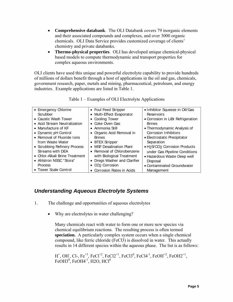
OLI clients have used this unique and powerful electrolyte capability to provide hundreds of millions of dollars benefit through a host of applications in the oil and gas, chemicals, government research, paper, metals and mining, pharmaceutical, petroleum, and energy industries. Example applications are listed in Table 1.

Table 1 – Examples of OLI Electrolyte Applications • Emergency Chlorine

Scrubber • Caustic Wash Tower • Acid Stream Neutralization • Manufacture of KF • Dynamic pH Control • Removal of Fluoride Ions

from Waste Water • Scrubbing Refinery Process

Streams with DEA • Chlor-Alkali Brine Treatment • Ahlstron NSSC “Stora”

Process • Tower Scale Control

• Foul Feed Stripper • Multi-Effect Evaporator • Cooling Tower • Coke Oven Gas • Ammonia Still • Organic Acid Removal in

Brines • BTEX Stripper • MSF Desalination Plant • Removal of Chlorobenzene

with Biological Treatment • Dregs Washer and Clarifier • CO2 Corrosion • Corrosion Rates in Acids

• Inhibitor Squeeze in Oil/Gas Reservoirs

• Corrosion in LiBr Refrigeration Brines

• Thermodynamic Analysis of Corrosion Inhibitors

• Electrostatic Precipitator Separation

• H2S/CO2 Corrosion Products under Gas Pipeline Conditions

• Hazardous Waste Deep well Disposal

• Contaminated Groundwater Management

Understanding Aqueous Electrolyte Systems 1. The challenge and opportunities of aqueous electrolytes

• Why are electrolytes in water challenging? Many chemicals react with water to form one or more new species via chemical equilibrium reactions. The resulting process is often termed speciation. A particularly complex system occurs when a single chemical compound, like ferric chloride (FeCl3) is dissolved in water. This actually results in 14 different species within the aqueous phase. The list is as follows: H+, OH-, Cl-, Fe+3, FeCl+2, FeCl2+1, FeCl30, FeCl4-1, FeOH+2, FeOH2+1, FeOH30, FeOH4-1, H2O, HCl0

And, the following independent equilibrium reactions are occurring in the aqueous phase: H2O = H+ + OH-

HCl0 = H+ + Cl- Fe+3 + Cl- = FeCl+2 FeCl+2 + Cl- = FeCl2+ FeCl2+ + Cl- = FeCl30 FeCl30 + Cl- = FeCl4-

Fe+3 + OH- = FeOH+2 FeOH+2 + OH- = FeOH2+ FeOH2+ + OH- = FeOH30 FeOH30 + OH- = FeOH4- The specific roster of species is usually confirmed by experimental means. This process of aqueous speciation via reaction, together with the physical equilibria with other phases can produce results, which are quite counter-intuitive. For example, one mole of ferric chloride dissolved in water produces a solution with pH of about 2, making ferric chloride in water a fairly strong acid. This non-intuitive result occurs because of the reactions, shown above, wherein OH- combines with Fe+3 via a series of stepwise reactions. This depletion of hydroxide ions then causes the water dissociation equilibrium reaction to move to the right liberating more hydrogen ions. Now, imagine the complexity of not just a single chemical compound in water but, rather, several or even many. The opportunity for equilibrium reactions abounds in such systems. One of literally uncountable examples of multi-component systems is the four-component system water-ammonia-carbon dioxide-hydrogen sulfide (See Appendix 1 for a more detailed discussion and comparison of OLI predicted and experimental results for this system). In this case, the list of species and reactions in the aqueous phase is as follows: H2O, H+, OH-, CO20, CO3-2, HCO3-, NH30, NH4+, NH2CO2-, H2S0, HS-, S-2 H2O = H+ + OH- CO20 + H2O = H+ +HCO3- HCO3- = H+ +CO3-2 NH30 + H2O = NH4+ + OH- NH2CO2- + H2O = NH4+ + CO3-2 H2S0 = H+ +HS- HS- = H+ + S-2 If one were to take the standard thermodynamic properties for the VLE between H2O, CO2, NH3, and H2S in the aqueous and gas phases and ignore the seven aqueous speciation equilibrium reactions shown above, the errors in

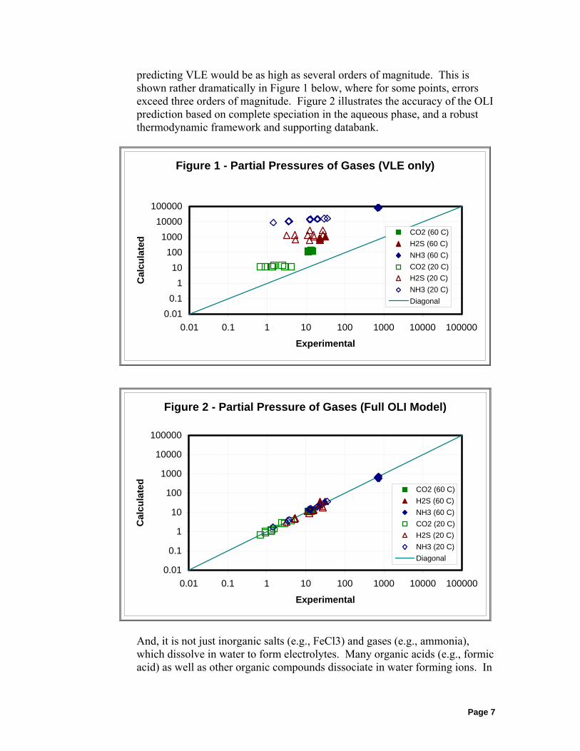
predicting VLE would be as high as several orders of magnitude. This is shown rather dramatically in Figure 1 below, where for some points, errors exceed three orders of magnitude. Figure 2 illustrates the accuracy of the OLI prediction based on complete speciation in the aqueous phase, and a robust thermodynamic framework and supporting databank.

Figure 1 - Partial Pressures of Gases (VLE only)

0.010.1

110

1001000

10000100000

0.01 0.1 1 10 100 1000 10000 100000

Experimental

Cal

cula

ted

CO2 (60 C)H2S (60 C)NH3 (60 C)CO2 (20 C)H2S (20 C)NH3 (20 C)Diagonal

Figure 2 - Partial Pressure of Gases (Full OLI Model)

0.01

0.1

1

10

100

1000

10000

100000

0.01 0.1 1 10 100 1000 10000 100000

Experimental

Cal

cula

ted


And, it is not just inorganic salts (e.g., FeCl3) and gases (e.g., ammonia), which dissolve in water to form electrolytes. Many organic acids (e.g., formic acid) as well as other organic compounds dissociate in water forming ions. In

addition, the resulting ions may form new species (called complexes, ion pairs, or organo-metallic complexes) by combining with metal ions. Many other organic compounds dissolve in water without dissociating. For almost all chemical compounds, which dissolve in water, there are limits to their solubility. And, this solubility varies when other chemical compounds are present as well. Any attempt to dissolve more than this solubility limit, results in partitioning of the chemical compound to another physical phase. At room temperature, for example, this may be a solid phase in the case of dissolving sodium chloride, a gas phase in the case of carbon dioxide, or a second liquid phase in the case of benzene. So, to get a complete picture of the thermophysical properties, speciation, and partitioning to other phases for a mixture of chemicals in water is a formidable challenge. The keys to solving this problem in the form of a predictive model are getting the speciation correct and then utilizing state-of-the-art models to represent the relevant thermodynamic properties of all species in the aqueous and related phases as well.

• Why are high ionic strength systems particularly problematic for less rigorous thermodynamic approaches? The previous section discussed the complexities of speciation for aqueous electrolyte systems. It is important to understand that these complexities are much more significant for systems with many components at high concentrations. Simplified approaches are sometimes used for very dilute systems, but these methods are not valid for higher concentration, multi-component systems typical of real industrial processes. For example, Figure 3 shows that the assumption of a unity activity coefficient (γ=1) can lead to large errors. At high concentration, interactions of ions and molecular species with each other and the solvent can become very significant and cannot be ignored. In addition, at high concentrations, the formation of complexes, as well as multi-component chemical interactions make accurate prediction difficult. The OLI framework is the only one in existence that incorporates a robust,

Figure 3

0.60

0.70

0.80

0.90

1.00

0 1 2 3 4 5 6NaCl (m)

ObservedPredicted

Na+ A

ctiv

ity C

oeffi

cien

t

Figure 4 Barium Sulfate Solubility

0

0.2

0.4

0.6

0.8

0 1 2 3 4 5 6

100 oC 150 oC 200 oC

Obs. Pred.

Solu

bilit

y (m

mol

es/k

g)

NaCl (moles/kg)

NaCl Solubility vs Pressure

26.0

26.5

27.0

27.5

28.0

0 5 10 15 20 25

Sol

ubilit

y (w

t %)

Pressure (psi x1000)

ObservedPredicted

predictive activity coefficient model that can accommodate these severe non-idealities. And, the OLI in-place Databank includes coefficients resulting from thousands of data regressions based on the best available thermodynamic data for binary and many ternary systems. Figure 4 illustrates the effect of temperature, pressure, and concentration, and the accuracy of OLI predictions.

• Why is aqueous electrolyte thermodynamics not well understood and broadly taught at the university level?

Until the culmination of more than 20 years of applied R&D at OLI, no one had put together a complete, speciation-based model for prediction of the thermophysical properties of aqueous-based systems over a broad range of conditions (e.g., -50C to 300C, 0 to 1500 bar, 0 to 30 molal). Key elements of the OLI model were developed over the past 100 years by Debye and Huckel, Helgeson, Pitzer, Meissner, and others. However, no one has put all of this together with key extensions and synthesized a model such as the OLI model. Thus, the OLI model is not generally known and understood at the university level.

• What benefits, features, capabilities, calculations, and functionality are

enabled only by a thorough understanding of aqueous electrolytes and what limitations and problems does a process/chemical engineer and a CPI company suffer by not understanding or considering aqueous electrolytes?

Consider a process application in which chlorine, a component of an off-gas product, is to be scrubbed with 10 % by weight sodium hydroxide solution. Several operating issues have evolved. Given the current design configuration, there is insufficient scrubbing efficiency. The plant operators increased the sodium hydroxide concentration from 10% by weight to 20% by weight. In addition, the Waste Liquid from the scrubber was desired to be at pH > 8.3 for alkalinity control. The result of the change in concentration was frequent fouling of the scrubber and an inability to control the pH. Using the OLI Electrolytes package, the plant operators found that increasing the concentration of sodium hydroxide to 20 % by weight did little to increase the scrubbing efficiency.

The amount of chlorine removal seems to be limited to approximately 50% at sodium hydroxide concentrations greater than 15% by weight. The plant operators also noticed that the column fouled frequently at the high concentrations of sodium hydroxide.

The off-gas contained carbon dioxide as well as chlorine. Using the OLI Electrolytes package, the plant operators found that sodium bicarbonate was created at the increased sodium hydroxide concentrations.

At the 20% by weight concentration of sodium hydroxide, sodium bicarbonate (a solid) begins to form. The plant operators confirmed the presence of this solid in their scrubber.

Another problem was that the pH could not be maintained at values greater that 8.3. The OLI Electrolytes package determined the pH response of the chemistry underlying the process.

The pH levels off at approximately 7.0 as the concentration of NaOH increases. This leveling effect, common in aqueous chemistry, is due the presence of solid NaHCO3 forming inside the scrubber. As long as this solid continues to form, the pH cannot

%Cl2 Removal v. Concentration of NaOH

0.00

20.00

40.00

60.00

0.00 10.00 20.00 30.00

wt% NaOH

%C

hlor

ine

Rem

oval

NaHCO3 Solid formation v. Concentration of NaOH

0

2

4

6

0.00 10.00 20.00 30.00

wt% NaOH

NaH

CO

3 so

lid

(mol

es)

pH v. Concentration of NaOH

0

2

4

6

8

0.00 5.00 10.00 15.00 20.00 25.00 30.00

wt% NaOH

pH

increase.

A lack of understanding aqueous electrolyte systems amongst engineers within the CPI area forces them to operate without the ability to predict the properties (e.g., pH) and phase separations associated with aqueous-based chemical systems. In a limited number of situations (e.g., sour water systems) there are some correlations available for predicting VLE or SLE for aqueous-based systems. Much more often designs and/or plant operations are based upon very conservative approaches (e.g., over-design) to avoid problems that could be predicted and avoided with the use of the OLI models. A typical example is scaling in tower units. The formation of salts can result in scale formation within a tower, which will reduce a tower's effectiveness and, eventually, require shutdown of the unit and, perhaps, even the plant. With the OLI model such salt formation in readily predicted leading to avoidance by altering operating conditions, the level of use of a reagent, or the addition of a scale inhibitor all of which can be predicted with the OLI model.

Aqueous Electrolytes Primer

A somewhat more detailed Aqueous Electrolyte Primer is given in Chapter 3. There are five principal partial molal properties in each phase about which we will be concerned. These are Gibbs Free Energy, Enthalpy, Entropy, Heat Capacity, and Volume. In particular, we will focus on the aqueous phase for which the thermodynamic approach is not well understood. The key to thermodynamic equilibrium, both aqueous intraphase speciation equilibria as well as the physical equilibria between phases is the Gibbs Free Energy (also called the Chemical Potential). For every thermodynamic equilibrium reaction the total Gibbs Free Energy for the species on the left-hand side of the reaction must be equal to the total Gibbs free energy on the right-hand side of the reaction. Thus: G-Left = G-Right (1) Where G is defined as the Total Gibbs Free Energy An example of such a reaction is: CO2o + H2O = H+ + HCO3- (2)

In this case: GCO2

o + GH2O = GH+ + GHCO3- (3)

The total Gibbs Free Energy can be further defined in terms of a Standard State Gibbs Free Energy (Go) and an activity (a) as follows: Gi = Gi

o + RT ln(ai) (4) Where R=Gas Constant and T is absolute temperature. Note that this classical definition is in terms of an activity rather than a concentration. To be able to write this in terms of concentration, we will have to introduce the notion of an activity coefficient, which captures the departure from ideality or, in other words, the relationship between the activity of a species and the concentration of that species. Thus, ai = γi * mi (5) Please note that the Greek symbol γ is used to denote the activity coefficient and the concentration unit molality (m) is usually used as the concentration unit for aqueous systems thermodynamics. Molality is defined as the number of moles of a species in a kilogram (approximately 55.508 moles) of water. Defining concentration in this way makes the concentration definition independent of density and, therefore, temperature.

The standard state used for aqueous-based systems is the one most commonly in use in the literature. For any species other than water, the standard state is the concentration of a hypothetical one-molal solution of the species extrapolated to infinite dilution. This standard state is termed asymmetrical and is a function of temperature and pressure only. Another way of writing equation (4) is: Gi = Gi

o + GiE (6)

Where the superscript E denotes the Excess Gibbs Free Energy and is therefore by equation (4) defined as RTln(a). The formidable challenge faced by researchers over the past century is how to write closed form equations as a function of temperature, pressure and concentration, which would predict the standard state and excess Gibbs Free Energy. This challenge reduces essentially to one of how to predict the standard state Gibbs Free Energy and activity coefficient for every (and, therefore any) possible species in water.

Before proceeding to the specific framework used by OLI, it is useful to point out that there are similar expressions to (6) for all five principal partial molal properties. Specifically, for the other four (Enthalpy, Entropy, Heat Capacity, and Volume), these expressions are: H = Ho + HE (7) S = So + SE (8)

Cp = Cpo + CpE (9) V = Vo + VE (10) We saw earlier that the excess term for the Gibbs Free Energy was directly related to the activity coefficient. For the other four properties, denoted above, the excess terms all relate to various partial derivatives of the activity coefficient. For example, the excess enthalpy directly relates to the first partial derivative of the activity coefficient with respect to temperature.

The OLI Thermodynamic Framework

OLI has developed a thermodynamic formulation for equations (6) - (10) above by utilizing the framework of Helgeson and co-workers for the standard state terms (the ones with the superscripts of "0") and the frameworks of Bromley, Zemaitis, Pitzer, Debye-Huckel, and others for the excess terms (the ones with the superscripts of "E"). The key to the predictive nature of the OLI model is based upon the work of Harold Helgeson and co-workers. Helgeson, a Professor of Geochemistry at UC Berkeley, has worked for 40 years to develop a predictive equation of state for the prediction of the partial molal standard state properties of any species within the aqueous phase. Co-workers such as Dimitri Sverjensky, now at Johns Hopkins University in the Department of Earth and Planetary Sciences, have contributed greatly to provide methods for estimating the coefficients of the equation of state for species where it is not practical to regress for the required coefficients. It is beyond the scope of this document to provide the specific formulas for the five principal standard state terms, however a general description is as follows:

Go = G(T, P, ω, c1, c2, a1, a2, a3, a4) Ho = H(T, P, ω, c1, c2, a1, a2, a3, a4) So = S(T, P, ω, c1, c2, a1, a2, a3, a4) Cpo = Cp(T, P, ω, c1, c2, a1, a2, a3, a4) Vo = V(T, P, ω, c1, c2, a1, a2, a3, a4)

The seven parameters shown in each equation are equation of state coefficients that are unique to each species. In many cases of interest to chemical engineers, a1 through a4 can be ignored since these coefficients relate only to the effects of pressure on the properties of interest and until pressures get above 100 atmospheres the effects of pressure are negligible. OLI has incorporated a Helgeson framework and estimation methods that allows data banking for the ω, c1, and c2 for virtually any species in water and, in most cases, a1 through a4 as well. Remember that equilibrium constants depend solely on the individual G0

values for the constituent species in each reaction. Since OLI, via its Helgeson framework, can predict these individual G0 values for any species in water, we can, therefore, predict any equilibrium constant. This fully predictive framework

for standard state properties relieves entirely the burden of speciation from the activity coefficients where, historically, this burden has been placed. Thus, the remaining compositional effects (called non-ideality) are placed, where they belong, on the activity coefficients without the added burden of speciation equilibrium. For the excess properties, as noted earlier, everything relates to the activity coefficients. OLI's model for activity coefficients of ions has the following form:

γ = DH(I) + BZ(I, T, m) where the first term DH is the so-called Debye-Huckel term, which is a function of I=ionic strength (this is the term that completely describes the activity coefficient for very dilute systems). The second term is the Bromley-Zemaitis term and is a function of ionic strength, temperature, and the individual species concentrations represented by m the vector of species molalities. The ionic strength is directly related to the various ionic concentrations.

Other Physical Phases in Equilibrium With the Aqueous Phase

The OLI model takes into account the possible occurrence of other phases and also provides databank support so that all required thermodynamic calculations are carried out automatically. Almost any possible solid that might form from an aqueous mixture is accounted for since the OLI code can consider, simultaneously, up to 250 possible solids that might precipitate from a mixture. In reality it is rare that more than 5 solids actually will precipitate at one time, but the model will correctly predict the precipitating solids. In addition the model accounts for the possible formation of a gas phase and a second (non-aqueous) liquid phase. The condition for physical equilibrium between phases is that the total Gibbs Free Energy (also known as chemical potential) is equal for the phases in equilibrium. Since we have already established the manner in which OLI calculates Gibbs Free Energy for the aqueous phase, we need only describe how OLI does this same calculation for solids, gases, and the second liquid phase. Each solid in equilibrium with the aqueous phase is an independent phase. Thus, we need only be able to calculate the Gibbs Free Energy for individual solids. This is done via classical thermodynamics by the equation: GS = GS

Tr + SSTr (T - Tr) + ∫CpdT + ∫VdP

Where, Tr is the Reference State temperature of 298.15K, and the two integrals are integrated from Tr to T.

For the gas and second liquid phase, OLI relies on an enhanced SRK formulation for the thermodynamic properties. For the free energy, the formulation is the classical formulation, which is: Gi = Gi

o + RTln(ficiP) Where, fi is the fugacity coefficient of species i in the gas or non-aqueous liquid phase and ci is the mole fraction of species i in the gas or non-aqueous liquid phase.

What OLI Provides

OLI provides all facilities, which enable a user to avoid all of the complexities associated with aqueous electrolyte systems. This means that the user never has to: • Write an equilibrium reaction • Define true species in the aqueous phase (the user only provides the

customary molecular chemical components) • Deal with any complexities associated with solving for the occurrence of other

physical phases in addition to the aqueous phase • Carry out any data regressions to develop model coefficients (these are all

provided by the in-place OLI databank)

Essentially, from a user point of view, the description of process streams and process units is no different than with conventional simulation. For example, using the highly complex system of H2O/FeCl3, described earlier, the user deals only with the two component system while the OLI software, behind the scenes deals with the 14 true species in solution, the 10 equilibrium reactions in the aqueous phase, and the physical equilibrium between the aqueous phase and any solid, vapor, and second liquid phase that may occur.

Range of Applicability of the OLI Model

There are a number of limitations of the OLI Model as follows:

• The temperature resulting from the equilibrium calculation must fall in the range -50 and 300 centigrade.

• The pressure resulting from the equilibrium calculation must fall in the range 0 and 1500 atmospheres.

• The mole fraction of water within the liquid phase resulting from the equilibrium calculation must fall in the range between 0.65 and 1.0.

• The OLI model used for the gas phase and second liquid phase is based upon an enhanced SRK equation of state. This means that certain non-ideal second liquid phases may not be represented well due to limits of the SRK.

• OLI has done data regression for an enormous number of chemical systems. Generally, all single components plus water have been regressed. Figure 5 illustrates the accuracy of typical binary system predictions at different temperatures. In addition, many ternary systems (water plus two other components) have been regressed together with the constituent binary systems. Figures 6 and 7 illustrate ternary system predictions compared to experimental data. (Also see Appendix 1 for other examples of data fits). Note particularly in Figure 7 the unusual behavior of gypsum at 25 ºC and high NaCl concentrations (there is a maximum gypsum solubility at an intermediate NaCl concentration). This behavior, accurately predicted by OLI, could not be predicted with less rigorous models. For regressed systems, the error between predicted and experimental values is generally less than 10%. Eventually, for all multi-component systems with more than three components plus water, OLI must rely on some estimation/prediction. The key to these systems is whether or not the subsystems defined by water together with components present in excess of 1 molal concentration have been subjected to data regression by OLI. If not, the predictions will usually be good qualitatively but fairly substantial errors (25+%) may occur in the actual predictions. For most common ternary systems (e.g., H2O/NH3/CO2, H2O/CO2/NaCl) it is safe to assume that OLI has done the required ternary system regressions. Well over 100 such systems have been regressed.

Figure 6

0

1

2

3

4

5

0 1 2 3 4NaCl (molal)

SrS

O4 S

olub

ility

(mm

olal

)

ObservedPredicted

71.1 oC

Figure 7

0

0.02

0.04

0.06

0 1 2 3 4 5 6 7

ObservedPredicted

Gypsum25 oC

Sol

ubilit

y (m

mol

/kg)

NaCl (mole/kg)

0

0.01

0.02

0 1 2 3 4 5 6

ObservedPredicted

200 oC

Sol

ubili

ty (m

mol

/kg)

NaCl (mole/kg)

Anhydrite

Figure 5 Calcite Solubility

Temperature (C)

012345678

100 150 200 250 300

0.5 m NaCl

ObservedPredicted

Sol

ubilit

y (m

mol

/kg)

Temperature (C)

012345678

100 150 200 250 300 350

1.0 m NaCl

ObservedPredicted

Sol

ubilit

y (m

mol

/kg)

012345678

100 150 200 250 300

Sol

ubilit

y (m

mol

/kg)

0.2 m NaCl

ObservedPredicted

The OLI Databank

OLI Electrolytes includes the Full Databank and the GeoChem Databank.

• Full databank

The full databank, listed in Appendix 3, covers thousands of species in water. In terms of inorganic chemistry this includes the much of the aqueous chemistry (including speciation reactions) for 79 elements from the Periodic Table in water. In addition, thousands of organic chemical compounds (electrolyte and non-electrolyte) are covered. OLI's mission is to cover any species that might of possible interest to our customers. The Full Databank delivers the results of much of this mission. However, where a customer finds that a species is missing or does not cover the range of conditions of interest, then the OLI Data Service (see below) takes over.

• Special databanks

In addition to the above-noted databank, OLI has a few other databanks that are generally distributed with the product. The Geochem databank (see list in Appendix 4) is separated from the public since it contains many solids, which only form via thermodynamic equilibrium after long periods of time (often thousands of years). There solids form in nature and are often different from the form of a solid, made up of the same elements, that may form in a much shorter amount of time (usually instantly) within a process. Thus, the Geochem solids tend to form through aging of the aqueous environment in contact with a source of the elements comprising the solids.

• Private (custom) databanks - OLI Data Service

The OLI Engine Software allows users to provide their own supplementary databanks (Private Databanks) in addition to the Public (Limited, Full and Special) databanks. These databanks can be prepared by users with special training but are normally prepared by the OLI Data Service. The procedure is that OLI is informed that certain chemistry either not covered or inadequately covered by the Full Databank, is required. OLI will then estimate the amount of time that it will take to do such a job, which leads to a quotation for performing the work. The fee quoted will vary based upon whether or not OLI can do the work based upon public domain information and whether or not OLI is free to release the results with subsequent releases of its Public Databanks. OLI's Data Service starts all projects with a thorough literature search. Then all relevant literature is critically reviewed and the experimental data, which is deemed fit is placed into computer files from which nonlinear regression is carried out. As a result of these regressions, databank coefficients are developed.

The OLI Engine

The OLI Engine is the essential heart of all OLI Software. The OLI Engine is defined as the databanks and solvers that enable the prediction and numerical solution of the underlying chemical and physical equilibria and, therefore, the thermophysical properties and phase separations for almost any mixture of chemicals in water at almost any conditions (T = -50 to 300 C, P = 0 to 1500 bar, Ionic Strength = 0 to 30 Molal) of practical interest to industry. The thermo-physical properties available in OLI Electrolytes are summarized in Table 2. In addition to the Thermodynamic Properties in Table 2, OLI has developed certain transport properties to support the rates of corrosion model. These properties include: viscosity, electrical conductivity and self-diffusivity.

Table 2 – Thermophysical Properties Available in OLI Electrolytes

Thermodynamic Properties Gibb’s Free Energy Enthalpy Entropy Heat Capacity Volume

pH Osmotic Pressure Ionic Strength Density Scaling Index

Chapter 2 Getting Started with Hysys OLI

Introduction The HYSYS OLI package (commonly referred to as HEO) can be used to study electrolyte solutions in a process simulator. In this simulation we will mix an acid and a base stream together and review the output.

Assumptions The user is expected to have adequate knowledge on starting, stopping and running Hysys. This includes process design and data entry.

Starting HYSYS OLI (HEO) Start HEO by following this path: Start > Programs > Hyprotech > Hysys 3.2 > Hysys Wait for the program to load the splash screen and then start the main window.

Figure 2

Starting a new case

Click the File > New > Case menu items. This will display the Basis Manager

Figure 3

Hysys requires the user to first select a Fluid Package before selecting components. This is not the first tab displayed but it is the first tab that needs to be selected. Click the Fluid Pkgs tab.

Figure 4

We now must add a fluid package. Click the Add… button.

Figure 5

Scroll down to find the OLI_Electrolyte Option

Figure 6

You can see that additional options are displayed when this package is selected. You may now close the window by clicking on the X.

Figure 7

We can now begin to select components Click on the Components… tab.

Figure 8

Select Component List –1 and click the View… button.

Figure 9

Select Electrolyte from the Add component tree

Figure 10

Enter H2O into the Match Box and press enter. All Electrolyte models require water (H2O) be selected.

Figure 11 (Before Enter is pressed)

Notice that the species listing scrolls to find your species. Now Press Enter.

Figure 12 After Enter

In this demonstration we will add hydrochloric acid (HCl) and sodium Hydroxide (NaOH). Enter both these species.

Figure 13

Entering the Simulation Environment. You can now close this window by clicking the X in the upper right-hand corner.

Figure 14

Click the Enter Simulation Environment…button.

Figure 15

We will now create a mix block with an acid feed and a base feed. Create the following streams Stream 1 Temperature 25 C Pressure 101.325 Kpa

Total Flow 100 Kg/Hr H2O 0.9 mole fraction HCL 0.1 mole Fraction Stream 2 Temperature 25 C Pressure 101.325 Kpa Total Flow 100 Kg/Hr H2O 0.9 mole fraction NAOH 0.1 mole Fraction Stream 3 is the outlet stream. Double-click Stream 3

Figure 16

Hysys OLI will calculate the streams as they are entered. In this case the results indicate a temperature rise to 75 .6 C. Save the file as required.

Chapter 3 Aqueous Thermodynamics

Overview Understanding aqueous thermodynamics can be a daunting task. In this chapter we will describe some of the essential topics in aqueous thermodynamics and present them in a logical, relatively easy to understand manner.

The Equilibrium Constant The evaluation of the following equation is central to the OLI Software:

∆ RoG RT K= − ln

Where ∆RoG is the partial molal, standard-state Gibbs Free Energy of

Reaction, R is the Gas Constant (8.314 J/mole/K), T is the temperature (Kelvin) and K is the equilibrium constant. The subscript R refers not to the gas constant but to an equilibrium reaction.

This refers to the total free energy, not just the standard-state portion.

We define ∆RG as:

∆ ∆ ∆R i

if i i f

iiG v G PRODUCTS v G REACTANTS= −∑ ∑( ) ( )

Where νi is the Stoichiometric coefficient and ∆ f iG is the Gibbs Free Energy of

Formation for a species.

Question: Consider the equilibrium:

Na2SO4 = 2Na+ + SO4

2- What is the Gibbs Free Energy of Reaction? What is the equilibrium constant at 25 oC (298.15K)1?

The reference state thermodynamic values are readily available:2 ∆ f

RG Na SO J mole( ) /2 4 1270100= − 3 ∆ f

RG Na J mole( ) /+ = −261800 ∆ f

RG SO J mole( ) /42 744460− = −

For the Gibbs Free Energy of reaction:

( )∆ ∆ ∆ ∆RR

fR

fR

fRG G Na G SO G Na SO= + −+ −2 4

22 4( ) ( ) ( )

( )∆ R

RG J mole= − + − − − =2 261800 744460 1270100 2640( ) ( ) ( ) / By rearranging our equilibrium equation we get:

ln KG

RTR R

R

= −∆

By now substituting the appropriate numbers we get:

ln KR = -(2640 J/mole) /((8.314 J/mole/K)(298.15K)) = -1.07 1 25oC (298.15K) is also know as the reference temperature. 2 NBS Tables of Chemical Thermodynamic Properties - Selected Values for Inorganic

and C1-C2 Organic Substances in SI Units, Wagman,D.D., et al, 1982 3 The subscript f refers the energy of formation from the elements. The superscript R refers to the reference state. This is a special case of the standard state normally denoted with a superscript o.

KR=0.34

Principal Thermodynamic Properties Each thermodynamic property is composed of two parts. The first is the standard state part which is only a function of temperature and pressure (denoted by the superscript o). The second is the excess part which is a function of temperature and pressure as well as concentration (denoted by the superscript E).

Partial Molal Gibbs Free Energy

G G Gi io

iE= +

Partial Molal Enthalpy E

ioii HHH +=

Partial Molal Entropy

S S Si io

iE= +

Partial Molal Heat Capacity

Cp Cp Cpi io

iE= +

Partial Molal Volume

V V Vi io

iE= +

Note: Superscript 0 = Standard State Property Superscript E = Excess Property

HKF (Helgeson-Kirkham-Flowers)Equation of State4,5

Working since 1968, Helgeson, et. al., have found that the standard-state thermodynamic property of any species in water can be represented by a function with seven terms which have specific values for each species.

4 H.C.Helgeson, D.H.Kirkham, G.C.Flowers. Theoretical Prediction of the Thermodynamic Behavior of Aqueous Electrolytes at High Pressures and Temperatures - Parts I through IV. American Journal of Science 1974, 1976, 1981. 5 J.C.Tanger, IV Doctorial Thesis. “Calculation of the Standard Partial Molal Thermodynamic Properties of Aqueous Ions and Electrolytes at High Pressures and Temperatures” University of California at Berkley, 1986 H.C.Helgeson Advisor.

These seven terms (a1-4, c1-2, and ω) are integration constants for volume (a), heat capacity (c ) and temperature and pressure properties of water ( ω). They are independent of the data system used to obtain them.

( )ω,,,,...., 2141 ccaafHH HiRi

oi +=

( ) ( )ω,,,,...., 2141 ccaafTTSGG GiRR

iRi

oi +−−=

( )ω,,,,...., 2141 ccaafSS SiRi

oi +=

( )ω,,,,...., 2141 ccaafCpCp CpiRi

oi +=

( )ω,,,,...., 2141 ccaafVV ViR

io

i +=

Superscript R - Reference State Property (25C, 1 bar) Superscript o - Standard State Property a1...a4 - Pressure Effects c1, c2 - Temperature Effects ω - Pressure, Temperature Effects

The Helgeson Equation of State Parameters are used to predict equilibrium constants.

Log K vs. Temperature HCO3

- = H+ + CO3-2

-14

-13.5

-13

-12.5

-12

-11.5

-11

-10.5

-10

-9.5

-9

0 50 100 150 200 250 300 350

Temperature (C)

Log

K

Figure 3-1 The logarithm of the equilibrium constant (LOG K) for the dissociation of the bicarbonate ion as a function of temperature at saturation pressure. The symbols represent the data taken from the references listed in the footnotes 6,7,8,9,10 but the line was generated from the equation of state.

6 H.S.Harned and S.R.Scholes. The Ionization Constant of HCO3

- from 0 to 50o. J.Am.Chem.Soc. 63,1706 (1941) 7 R.Nasanen. Zur Einwirkung der Saure und Basenzusatze auf die Fallungskurvevon Bariumcarbonate. Soumen Kemistilehti 90,24 (1946) 8 F. Cuta and F.Strafelda. The second dissociation constant of carbonic acid between 60 and 90oC. Chem. Listy 48,1308 (1954) 9 B.N.Ryzhenko. Geochemistry International 1,8 (1963) 10 C.S.Patterson, G.H.Slocum, R.H.Busey and R.E.Mesmer. Carbonate equilibrium in hydrothermal systems: First ionization of carbonic acid in NaCl media to 300oC. Geoch.Cosmoh.Acta 46,1653 (1982)

The Helgeson Equation of State Enthalpy

( ) ( ) ⎟⎟⎠

⎞⎜⎜⎝

⎛+Ψ+Ψ

+−+⎥⎦

⎤⎢⎣

⎡⎟⎟⎠

⎞⎜⎜⎝

⎛Θ−

−⎟⎠⎞

⎜⎝⎛

Θ−−−+∆=∆

rr

rr

of

oTP P

PaPPaTT

cTTcHH ln112121,

( )( ) Pr

r TTTY

TT

PPaPPa ⎟

⎠⎞

⎜⎝⎛∂∂

⎟⎠⎞

⎜⎝⎛ −−+⎟

⎠⎞

⎜⎝⎛ −+⎥

⎦

⎤⎢⎣

⎡

Θ−Θ−

⎟⎟⎠

⎞⎜⎜⎝

⎛⎥⎦

⎤⎢⎣

⎡+Ψ+Ψ

+−+ω

εω

εω 11112ln 243

rrTrTr

Tr YTPr,Pr,

Pr, 11 ωε

ω −⎟⎟⎠

⎞⎜⎜⎝

⎛−−

Gibbs Free Energy

( ) ( ) ⎟⎟⎠

⎞⎜⎜⎝

⎛+Ψ+Ψ

⎟⎟⎠

⎞⎜⎜⎝

⎛+Ψ+Ψ

+−+⎥⎦

⎤⎢⎣

⎡+−⎟⎟

⎠

⎞⎜⎜⎝

⎛−−−∆=∆

rrrr

rr

oTr

of

oTP P

PPPaPPaTT

TTTcTTSGG lnln 211Pr,,

( ) ( )( ) ⎥

⎥⎦

⎤

⎢⎢⎣

⎡⎟⎟⎠

⎞⎜⎜⎝

⎛Θ−Θ−

Θ−⎟

⎠⎞

⎜⎝⎛

Θ−Θ

⎟⎟⎠

⎞⎜⎜⎝

⎛⎟⎟⎠

⎞⎜⎜⎝

⎛Θ−

−⎟⎠⎞

⎜⎝⎛

Θ−−⎟

⎠⎞

⎜⎝⎛

Θ−⎥⎦

⎤⎢⎣

⎡⎟⎟⎠

⎞⎜⎜⎝

⎛+Ψ+Ψ

+−+r

r

rrr TT

TTTTTT

cTP

PaPPa ln111ln 2243

( )rTrTrTr

Tr TTY −+⎟⎟⎠

⎞⎜⎜⎝

⎛−−⎟

⎠⎞

⎜⎝⎛ −+ Pr,Pr,

Pr,Pr, 1111 ω

εω

εω

Volume

T

o

PQ

TPaa

PaaV ⎟

⎠⎞

⎜⎝⎛∂∂

⎟⎠⎞

⎜⎝⎛ −+−⎟

⎠⎞

⎜⎝⎛

Θ−⎥⎦

⎤⎢⎣

⎡⎟⎠⎞

⎜⎝⎛

+Ψ++⎟

⎠⎞

⎜⎝⎛

+Ψ+=

ωε

ω 111114321

Heat Capacity at Constant Pressure

( )( )

pPrr

o

TT

TTYTX

PPaPPa

TT

TccCp ⎟⎟

⎠

⎞⎜⎜⎝

⎛∂∂

⎟⎠⎞

⎜⎝⎛ −−⎟

⎠⎞

⎜⎝⎛∂∂

++⎥⎦

⎤⎢⎣

⎡⎟⎟⎠

⎞⎜⎜⎝

⎛+Ψ+Ψ

+−⎟⎟⎠

⎞⎜⎜⎝

⎛

Θ−−⎟

⎠⎞

⎜⎝⎛

Θ−+= 2

2

433

2

21 112ln21 ωε

ωω

Entropy ( )( ) ( ) ⎥

⎦

⎤⎢⎣

⎡⎟⎟⎠

⎞⎜⎜⎝

⎛+Ψ+Ψ

+−⎟⎠⎞

⎜⎝⎛

Θ−+

⎭⎬⎫

⎩⎨⎧

⎟⎟⎠

⎞⎜⎜⎝

⎛Θ−Θ−

Θ+⎟⎟

⎠

⎞⎜⎜⎝

⎛Θ−

−⎟⎠⎞

⎜⎝⎛

Θ−Θ−+=

rr

r

r

rt

oTr

o

PPaPPa

TTTTT

TTc

TTcSS ln1ln111ln 43

22

1Pr,

TrTrP

YT

Y Pr,Pr,11 ωωε

ω −⎟⎠⎞

⎜⎝⎛∂∂

⎟⎠⎞

⎜⎝⎛ −−+

Where H = Enthalpy G = Gibbs Free Energy

V = Volume Cp = Heat Capacity at constant Pressure S = Entropy T = Temperature P = Pressure Θ = 228 K Ψ = 2600 Bar ω = Temperature and Pressure dependent term for electrostatic nature of the electrolytes Q = Pressure functions of the dielectric constant ε = Dielectric constant of water a1,…,a4 = Pressure dependent terms c1, c2 = Temperature dependent terms What is the standard State?

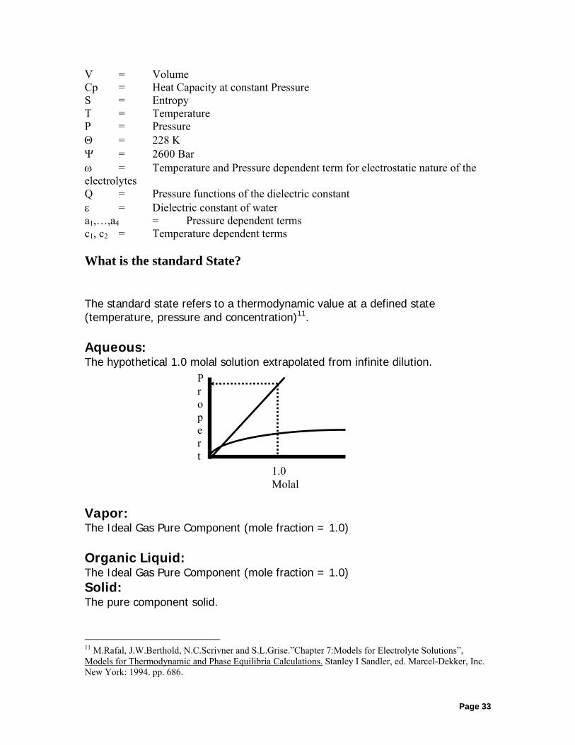
The standard state refers to a thermodynamic value at a defined state (temperature, pressure and concentration)11. Aqueous: The hypothetical 1.0 molal solution extrapolated from infinite dilution. Vapor: The Ideal Gas Pure Component (mole fraction = 1.0) Organic Liquid: The Ideal Gas Pure Component (mole fraction = 1.0) Solid: The pure component solid.

11 M.Rafal, J.W.Berthold, N.C.Scrivner and S.L.Grise.”Chapter 7:Models for Electrolyte Solutions”, Models for Thermodynamic and Phase Equilibria Calculations. Stanley I Sandler, ed. Marcel-Dekker, Inc. New York: 1994. pp. 686.

1.0Molal

Propert

Excess Properties Excess properties are a function of temperature, pressure and composition. It is with the excess properties that we begin to introduce the concept of activities and activity coefficients. The excess property that we are most concerned with is the excess Gibbs Free Energy: The activity of a species in solution can be defined as:

iii ma γ=

io

i a RTG = G ln+

iio

i RTm RTG = G γlnln ++

iEi RT = G γln

Note: Other excess properties involve various partial derivatives of γi with respect to temperature and/or pressure.

H RTTi

E i

P

=⎤⎦⎥

2 δ γδln

Ionic Strength Ionic Strength is defined by the following equation:

where, nI = number of charged species

I = 1 / 2 ( z m )i=1

nI

i2

i∑

For Example, a 1.0 molal solution of NaCl has 1.0 moles of Na+1 ion and 1.0 moles of Cl-1 ion per Kg H2O.

( ) ( ) ( ) ( )( ) ( ) ( ) ( ) ( )( ) 1111121

21 2222

1111 =−+=+= +−++ ClClNaNamZmZI

Therefore the ionic strength is 1.0 molal. For Example, a 1.0 molal solution of CaCl2 has 1.0 moles of Ca+2 ion and 2.0 moles of Cl-1 ion per Kg H2O.

( ) ( ) ( ) ( )( ) ( ) ( ) ( ) ( )( ) 3211221

21 2222

1122 =−+=+= +−++ ClClCaCa mZmZI

There for the ionic strength is 3.0 molal, or we can say that a 1.0 Molal solution of CaCl2 behaves similar to a 3.0 molal Solution of NaCl Definition of Aqueous Activity Coefficients

log γi = long range + short range

Long Range: Highly dilute solutions (e.g., 0.01 m NaCl). The ions are separated sufficiently such that the only interactions are between the ions and the solvent.

Short Range: Increased concentrations. The ions are now beginning to

interact with themselves (oppositely charged species attract, like charged species repel) in addition to the interactions with the solvent.

Long Range Terms

ln( )

( )γ i

z A T I

B T I=

−

+

2

1 Å

Å ion size parameter

A(T), B(T) Debye-Huckel parameters related to dielectric constant of water.

At 25 oC and 1 Atmosphere12: A(T) = 0.5092 kg1/2/mole1/2 B(T) = 0.3283 kg1/2/mole1/2-cm x10-8

12 H.C.Helgeson and D.H.Kirkham. American Journal of Science Vol. 274, 1199 (1974)

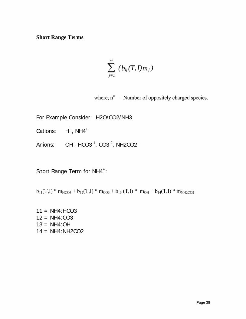
Short Range Terms

where, no = Number of oppositely charged species. For Example Consider: H2O/CO2/NH3 Cations: H+, NH4+

Anions: OH-, HCO3-1, CO3-2, NH2CO2- Short Range Term for NH4+: b11(T,I) * mHCO3 + b12(T,I) * mCO3 + b13 (T,I) * mOH + b14(T,I) * mNH2CO2 11 = NH4:HCO3 12 = NH4:CO3 13 = NH4:OH 14 = NH4:NH2CO2

j=1

n

ij j

o

(b (T,I)m )∑

Modern Formulations 1. Bromley - Meissner : Semi-Correlative13,14 Can predict and extrapolate excess properties when data is limited or unavailable. 2. Pitzer: Highly Interpolative15 Somewhat model dependent. Considerable caution is required when using the large amount of published data to verify the standard state model employed.

3. Helgeson: Limited in Scope16 Bromley

( )BI

ZZI

IZZBI

IZZALog +

⎟⎟⎠

⎞⎜⎜⎝

⎛+

++

+

−=

−+

−+−+± 2

||5.11

||6.006.01

||γ

Where A = Debye-Huckel Constant I = Ionic Strength B = Bromley parameter γ = Mean activity coefficient Z+ = Charge of the cation Z- = Charge of the anion Bromley-Zematis Joseph Zematis, formerly of OLI Systems, Inc., now deceased, extended the work of Bromley in that he added two new terms17. The Bromley-Zematis activity model is:

13 L.A.Bromley. J.Chem.Thermo.,4,669 (1972) 14 H.P.Meissner. AIChE Symp.Ser.No. 173,74,124 (1978) 15 K.S.Pitzer,et.al. J.Soln.Chem,4,249(1975); J.Phys.Chem.,81,1872(1977); J.Soln.Chem. 7,327(1978); J.Am.Chem.Soc.96,5701(1974) 16 H.C.Helgeson, D.H.Kirkham and G.C.Flowers. Am.J.Sci. 281,1249(1981) 17 Zemaitis, J.F., Jr, Clark, D.M., Rafal, M. and Scrivner, N.C., Handbook of Aqueous Electrolyte Thermodynamics, American Institute of Chemical Engineers, New York, 1986.

( ) 322

||5.11

||6.006.01

|| DICIBI

IZZ

IZZBI

IZZALog +++

⎟⎟⎠

⎞⎜⎜⎝

⎛+

++

+−

=

−+

−+−+±γ

Where C and D are new terms. Each of the B, C, and D terms have the following temperature functionality.

2321 TBTBBB ++= (Where T is temperature in centigrade)

The other coefficients have the same form: 2

321 TCTCCC ++= 2

321 TDTDDD ++=

Pitzer ( ) ( ) γγγ

ννν

νννγ ±

−+±

−+−+± ⎟⎟

⎠

⎞⎜⎜⎝

⎛+⎟⎟

⎠

⎞⎜⎜⎝

⎛+= CmBmfZZ

5.12 22||ln

Where fγ = The “Debye-Huckel” term.18 ν+ = Stoichiometric coefficient for the cation ν- = Stoichiometric coefficient for the anion ν = ν+ + ν- m = Concentration in molal γ

±B = Pitzer B term, containing the adjustable parameters γ

±C = Pitzer C term, containing adjustable parameters Helgeson

⎟⎟

⎠

⎞

⎜⎜

⎝

⎛

Ψ+

Ψ++Γ+

+

−= ∑∑∑±

i i

iil

k

kl

l l

lil

k

ki

kkk

k

kli IYbIYbIYbIBa

IZZALog

νν

νν

νω

γγ γ

γ ,,

01

||

Where Aγ = Debye-Huckel constant according to Helgeson Zi = Charge on the cation Zl = Charge on the anion a0 = ion size parameter Bγ = Extended Debye-Huckel term according to Helgeson

I = True ionic strength which includes the effects of complexation

18 IBID, Page 74

Γγ = Conversion of molal activity to mole fraction activity ωk = Electrostatic effects on the solvent due to the species k νk = moles of electrolyte (summation) νi,k = moles of cation per mole of electrolyte νl,k = moles of anion per mole of electrolyte bi,l = adjustable parameter for the ion-ion interaction.

iY = fraction of ionic strength on a true basis attributed to the cation

lY = fraction of ionic strength on a true basis attributed to the anion Ψi = ½ the cation charge Ψl = ½ the anion charge Zi = the cation charge Zl = the anion charge

Neutral Species Neutral molecules in water are affected by other species in solution. The salting in and out of a gas is a typical example. When Oxygen is dissolved into pure water, it has a typical solubility. When salt is added, the solubility decreases. This is most-likely due to an interaction between the sodium ions and the neutral oxygen molecule and the interaction between the chloride ions and the neutral oxygen molecule.

Figure 3-2 The solubility of oxygen in NaCl solutions at 25 C, 1 Atmosphere

Setschenow19 This characterizes a phenomena known as salting in/out. The formulation is in terms of the ratio of solubilities in pure water to an aqueous salt solution at a constant temperature.

SS

aq kmSSLn == 0γ

Where S0 = Solubility of the gas in pure water SS = Solubility of the gas in a salt solution K = Setschenow coefficient ms = Concentration of the salt. In this case, the K is approximately = -0.0002 Unfortunately, this approach is limited to a single temperature.

19 J.Setchenow., Z.Physik.Chem., 4,117 (1889)

Pitzer20 A more rigorous approach than Setschenow. Effects of temperature and composition can be modeled.

ssmmmmaq mmLn )(0)(0 22 −− += ββγ

Where

β0(m-m) = The adjustable parameter for molecule – molecule interactions.

(a function of temperature) β0(m-s) = The adjustable parameter for molecule

– ion interactions. (A function of temperature) mS = The concentration of the neutral species.

Multiphase Model Solid-Aqueous Equilibrium General Equilibrium Form Si = p1 P1 + p2 P2 + ... pp Pp Examples NaCl(cr) = Na+ (aq) + Cl-(aq) CaSO4.2H2O(cr) = Ca+2(aq) + SO4-2(aq) + 2H2O

20 K.S.Pitzer,et.al. J.Soln.Chem,4,249(1975); J.Phys.Chem.,81,1872(1977); J.Soln.Chem. 7,327(1978); J.Am.Chem.Soc.96,5701(1974)

Solid Phase Thermodynamic Properties

G G S T T CpdT VdPSi SiR

SiR R

T

T

P

P

R R

= + − + +∫ ∫( )

Cp = a1 + a2T + a3T-2 Under the conditions normally simulated, the compressibility of the solid remains constant.

V = b1

Log10Ksp(T,P) = A + B/TK + CTK + DT2

K + E + FP + GP2 Mixed EOS Model

General Thermodynamic Equation Vapor-Aqueous

iV AqiG = G

Vio

Vi i Aqio

i iG + RTln( y P) = G + RTln( m )φ γ Aqi i ia = mγ Vi Vi if = y Pφ

The reference state for the vapor is the ideal gas.

Vio

Vi Aqio

AqiG + RTln( f ) = G + RTln( a )

K = [( G - G )

RT] =

af

Aqio

Vio

Aqi

ViEXP

Non-Aqueous Liquid-Aqueous

Li AqiG = G Notice that the reference state for the non-aqueous liquid is the ideal gas vapor.

Vio

Li i Aqio

i iG + RTln( x P) = G + RTln( m )φ γ

Li Li if = X Pφ Vi

oLi Aqi

oAqiG + RTln( f ) = G + RTln(a )

K = [(G - G )

RT] =

af

Aqio

Lio

Aqi

LiEXP

Limitations of the Current OLI Thermodynamic Model Aqueous Phase XH2O > 0.65 -50oC < T < 300oC 0 Atm < P < 1500 Atm 0 < I < 30 Non-aqueous Liquid Currently no separate activity coefficient Model (i.e., no NRTL, Unifaq/Uniqac) Non-aqueous and vapor fugacity coefficients are determined from the Enhanced SRK21 Equation of State. Vapor critical parameters (Tc, Pc, Vc, and ω22) are correlated to find a Fugacity coefficient.

Scaling Tendencies What is a scaling tendency? It is the ratio of the real-solution solubility product to the thermodynamic limit based on the thermodynamic equilibrium constant. For Example, Consider this dissolution NaHCO3(s) = Na+ + HCO3-

The Ion Activity Product (IAP) is defined as the product of specific ions (in this case the ions resulting from the dissociation of a particular solid).

Let’s consider a 1.0 molal NaHCO3 solution:

IAP = γNamNaγHCO3mHCO3

21 G.Soave.Chem.Eng.Sci.27,1197(1972) 22 This is the acentric factor which is not the same as Helgeson’s ω term)

Assuming Ideal Solution Activities

γNa = 1.0 γHCO3 = 1.0

mna = 1.0 mHCO3 = 1.0

IAP = (1.0)(1.0)(1.0)(1.0)

IAP = 1.0 The Solubility Product (KSP) is the thermodynamic limit of ion availability

Ksp = γNamNaγHCO3mHCO3

KSP = 0.403780 The Scaling Tendency is then the ratio of available ions to the thermodynamic limit.

ST = IAP/KSP ST = 1.0/0.403780 ST = 2.48 Was assuming ideal conditions valid?? The actual species concentration and activity coefficients are:

γNa = 0.598 γHCO3 = 0.596 mna = 0.894 mHCO3 = 0.866 This results in a different IAP

IAP= (0.598)(0.894)(0.596)(0.866) IAP=0.276

The new Scaling Tendency is therefore: ST = IAP/Ksp ST = 0.276/0.40378 ST = 0.683 Why are the concentrations not equal to 1.0? Speciation and chemical equilibria tend to form complexes which provide a “Sink” for carbonate species. In this example:

CO2o = 0.016 molal

NaHCO3o = 0.101 molal CO32- = 0.012 molal NaCO3- = 0.004 molal

What does the Scaling Tendency Mean?

•

If ST < 1, then the solid is under-saturated If ST > 1, then the solid is super-saturated If ST = 1, then the solid is at saturation Scaling Index = Log (ST)

What is the TRANGE? TRANGE is a the nomenclature for solids that have been fit to a polynomial form rather than pure thermodynamics. The polynomial has this functional form:

Log K = A + B/T + CT + DT2

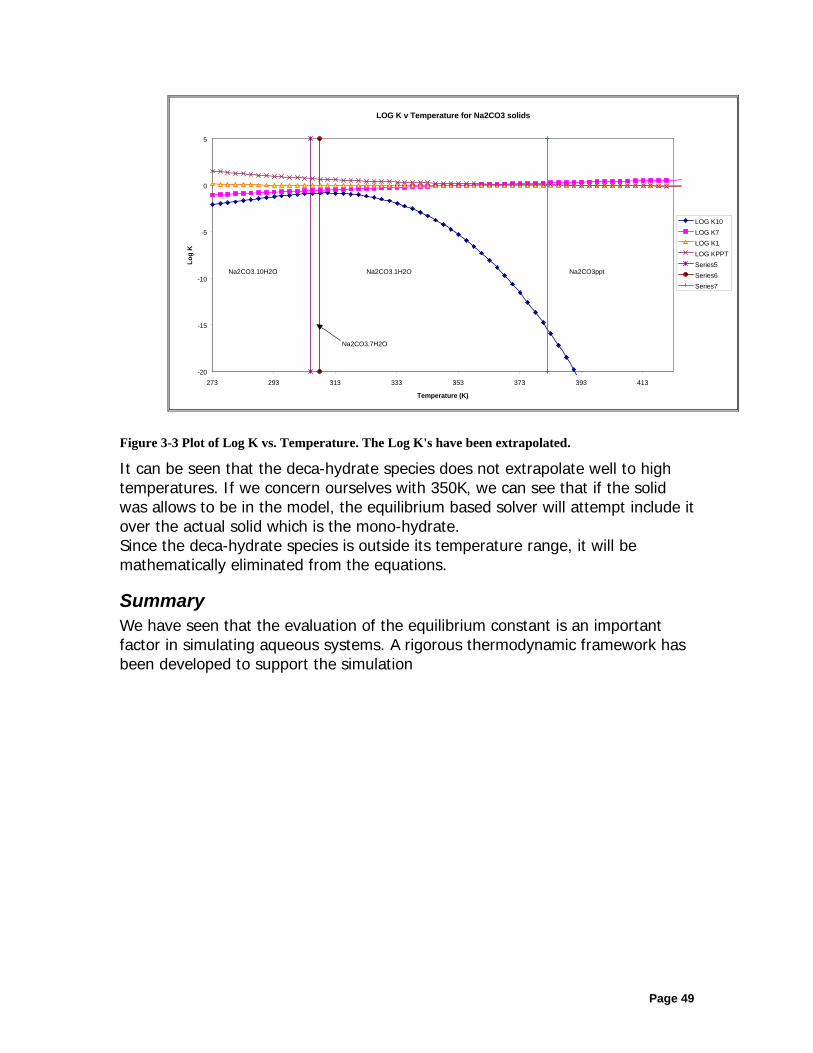
It is known that polynomials may not extrapolate well. Incorrect predictions of Scaling Tendency may result. Therefore the applicable range is generally limited to data set. Consider Na2CO3/H2O There are 4 solids of interest in this system. They are:

Solid Temperature Range (C) Na2CO3•10H2O 0-35 Na2CO3•7H2O 35-37 Na2CO3•1H2O 37-109

Na2CO3 109-350 This table implies that these solids change their form as the temperature increases. Each solid was fit to the above polynomial. There may be problems if the extrapolated values from higher number hydrates extend to the regions where the lower number hydrates are stable.

LOG K v Temperature for Na2CO3 solids

-20

-15

-10

-5

0

5

273 293 313 333 353 373 393 413

Temperature (K)

Log

K

LOG K10LOG K7LOG K1LOG KPPTSeries5Series6Series7

Na2CO3.10H2O

Na2CO3.7H2O

Na2CO3.1H2O Na2CO3ppt

Figure 3-3 Plot of Log K vs. Temperature. The Log K's have been extrapolated.

It can be seen that the deca-hydrate species does not extrapolate well to high temperatures. If we concern ourselves with 350K, we can see that if the solid was allows to be in the model, the equilibrium based solver will attempt include it over the actual solid which is the mono-hydrate. Since the deca-hydrate species is outside its temperature range, it will be mathematically eliminated from the equations.

Summary We have seen that the evaluation of the equilibrium constant is an important factor in simulating aqueous systems. A rigorous thermodynamic framework has been developed to support the simulation

Chapter 4 Examples of OLI Prediction Accuracy

Solubility Prediction

Barite Data OLI Electrolytes accurately predicts the barite solubility over broad ranges of temperatures, pressures, and salinities.

0

0.2

0.4

0.6

0.8

0 1 2 3 4 5 6

100 oC 150 oC 200 oC

Obs. Pred.

Sol

ubili

ty (m

mol

es/k

g)

NaCl (moles/kg)

Sodium Chloride Data OLI’s extensive database allows for prediction of virtually all industrially important solids. Below is a plot of the observed versus predicted solubility of NaCl over a broad range of pressures.

26.0

26.5

27.0

27.5

28.0

0 5 10 15 20 25

Sol

ubilit

y (w

t %)

Pressure (psi x1000)

ObservedPredicted

Celestite Data Based upon quality fits, OLI Electrolytes software produces accurate predictions of strontium sulfate (celestite) solubility under a variety of conditions. In the two graphs shown below, celestite solubility is predicted at two separate temperatures, 25 and 71.1 °C. over the solubility range of NaCl (0 to 6 molal).

0

1

2

3

4

5

0 1 2 3 4NaCl (mole/kg)

ObservedPredicted

71.1 oC

Sol

ubilit

y (m

mol

/kg)

NaCl (mole/kg)0 1 2 3 4 5

ObservedPredicted

25 oC

0

1

2

3

4

5

Sol

ubili

ty (m

mol

/kg)

Temperature (C)

012345678

100 150 200 250 300

0.5 m NaCl

ObservedPredicted

Sol

ubili

ty (m

mol

/kg)

Temperature (C)

012345678

100 150 200 250 300 350

1.0 m NaCl

ObservedPredicted

Sol

ubili

ty (m

mol

/kg)

012345678

100 150 200 250 300

Sol

ubili

ty (m

mol

/kg)

0.2 m NaCl

ObservedPredicted

Calcite Solubility versus Temperature The following graphs illustrate, the experimental and predicted solubility of calcite at high temperatures, pressures, and NaCl concentrations. As shown, the software accurately predicts calcite solubility over all conditions. This is due to the rigorous approach to computing the thermodynamic solubility of CaCO3 and the activity coefficients for the complete speciation of the ions in solution.

Gypsum and Anhydrite Data OLI software produces accurate predictions of calcium sulfate solubility under a variety of conditions for the two major crystalline phases. In the two graphs shown below, gypsum (CaSO4.2H2O) and anhydrite (CaSO4) solubility is predicted over the NaCl range of 0 to 6 molal.

0

0.02

0.04

0.06

0 1 2 3 4 5 6 7

ObservedPredicted

Gypsum25 oC

Sol

ubili

ty (m

mol

/kg)

NaCl (mole/kg)

0

0.01

0.02

0 1 2 3 4 5 6

ObservedPredicted

200 oC

Sol

ubilit

y (m

mol

/kg)

NaCl (mole/kg)

Anhydrite

Speciation in Sour Water For the sour water system (NH3/H2S/CO2/H2O) with Sour Water Species as follows:

Vapor Species: H2O, CO2, H2S and NH3 Aqueous Neutral Species: H2O, CO2, H2S and NH3 Aqueous Ionic Species: H+, OH-, NH4

+, HS-, S2-, HCO3-, CO3

2-, and NH2CO2-

The chemistry can be summarized as:

Vapor - Liquid Equilibrium Reactions (Molecular Equilibrium) H2O(vap) = H2O NH3(vap) = NH3(aq) CO2(vap) = CO2(aq) H2S(vap) = H2S(aq)

Aqueous Chemical Reactions (Electrolyte Equilibrium) – Note additional electrolyte reactions are needed.

H2O = H+ + OH- NH3(aq) + H2O = NH4

+ + OH- CO2(aq) + H2O = H+ + HCO3

- HCO3

- = H+ + CO32-

NH2CO2- + H2O = NH3(aq) + HCO3

- (Notice that this is the hydrolysis of an ion) H2S(aq) = H+ + HS- HS- = H+ + S2-

This example illustrates both the importance of considering the aqueous reactions and speciation, as well as the agreement of OLI predictions with experimental data. The data contained in Table 1 compares the experimental partial pressures of carbon dioxide, ammonia and hydrogen sulfide against a VLE only model and the full OLI speciated model.

Liquid Concentration

(molality) Partial Pressure (mmHg) NH3 CO2 H2S Temp (C) NH3 CO2 H2S Exper. OLI VLE Exper. OLI VLE Exper. OLI VLE

2.076 1.516 0.064 14.74

4 12.388 121.6751.48

8592.19

2 79594.8 31.616 36.936 1033.6

60 2.098 1.601 0.052 13.60

4 10.792 129.2738.11

2744.57

2 84762.8 23.256 35.112 843.6

1.954 1.471 0.04 11.47

6 11.172 114691.90

4 638.4 76820.8 22.8 25.004 638.4 2.16 1.581 0.05 13.68 12.92 129.2 705.28 590.52 83524 22.42 28.12 813.2 1.231 0.424 0.196 4.104 3.648 12.16 1.444 1.672 8580.4 3.192 3.04 1292

1.236 0.507 0.201 2.888 2.66 12.16 3.496 3.42 10290.4 5.092 4.484 1325.44 1.45 0.517 0.407 2.432 2.736 14.44 3.724 4.028 10526 12.54 10.944 2690.4 1.439 0.665 0.396 1.52 1.444 14.44 13.072 13.148 13611.6 26.98 20.672 2634.16

20 1.132 0.681 0.1 1.368 1.216 11.4 12.16 13.984 13892.8 5.32 4.94 663.48 1.234 0.694 0.199 1.292 1.216 12.16 13.072 16.036 14181.6 11.172 11.096 1322.4

1.238 0.712 0.203 1.292 1.064 12.16 19 18.62 14561.6 15.276 12.464 1345.2 1.234 0.725 0.199 0.912 0.988 12.16 20.444 20.672 14835.2 15.96 13.072 1079.2 1.235 0.771 0.2 0.912 0.836 12.16 29.184 30.324 15808 27.36 17.024 1333.04 1.126 0.794 0.095 0.684 0.684 11.4 35.188 36.252 16271.6 12.236 8.892 633.08

Table 1 - Comparing Experimental Partial Pressures to Calculated values.

Partial Pressures of Gases (VLE only)

0.010.1

110

1001000

10000100000

0.01 0.1 1 10 100 1000 10000 100000

Experimental

Cal

cula

ted CO2 (60 C)

H2S (60 C)NH3 (60 C)CO2 (20 C)H2S (20 C)NH3 (20 C)Diagonal

Figure 1 - Parity plot of the partial pressures of gases without aqueous reactions In Figure 1, the calculated partial pressures of the gases are over predicted. In the case of ammonia (filled and open diamonds), the over prediction may be as much a five orders of magnitude. If the OLI full speciation approach is not followed, this data can be improved with statistical corrections or by applying a strong activity model. These corrections, however, may work for this set of conditions. But if conditions other than the conditions in these series of calculations are desired, then these “corrections” will not be valid. The OLI approach using full speciation is predictive over the entire range of OLI model conditions.

Partial Pressure of Gases (Full OLI Model)

0.01

0.1

1

10

100

1000

10000

100000

0.01 0.1 1 10 100 1000 10000 100000

Experimental

Cal

cula

ted


Figure 2 - Parity plot of the partial pressures of gases with aqueous reactions When all the equilibria are included in the calculations, the calculated partial pressure of the gases agrees with the experimental values (Figure 2). This was done without specialized data regression to the general range of this data. This provides confidence that the predictions will hold at other conditions.

getting started with hysys oli

Documents