Gerris: a tree-based adaptive solver for the

incompressible Euler equations in complex

geometries

Stephane Popinet

National Institute of Water and Atmospheric Research, PO Box 14-901 Kilbirnie,

Wellington, New Zealand

Abstract

An adaptive mesh projection method for the time-dependent incompressible Eulerequations is presented. The domain is spatially discretised using quad/octrees anda multilevel Poisson solver is used to obtain the pressure. Complex solid boundariesare represented using a volume-of-fluid approach. Second-order convergence in spaceand time is demonstrated on regular, statically and dynamically refined grids. Thequad/octree discretisation proves to be very flexible and allows accurate and efficienttracking of flow features. The source code of the method implementation is freelyavailable.

Key words: Incompressible flow, adaptive mesh refinement, approximateprojection method, complex geometry1991 MSC: 65M06, 65N06, 65N55, 76D05, 76-04

1 Introduction

Efficient techniques for the numerical simulation of low Mach number flows have a largerange of applications: from fundamental fluid mechanics studies such as turbulence orinterfacial flows, to engineering and environmental problems. For time-dependent flows,the finite speed of propagation of sound waves can lead to strong restrictions on themaximum value of the timestep. While filtering techniques can be applied to try tolift this constraint, a better approach is to assume that the fluid considered is strictlyincompressible. This introduces an elliptic problem for the pressure which expressesthe instantaneous propagation of pressure information throughout the entire domain.In practice, this leads to the fundamental change from a spatially explicit to a spatiallyimplicit problem.

Email address: s.popinet@niwa.co.nz (Stephane Popinet).

Preprint submitted to Journal of Computational Physics 1 July 2003

Projection methods and multigrid solvers have proved an efficient combination to solvethis type of problem [1–4]. More recently, these techniques have been extended throughthe use of higher-order, unconditionally stable advection schemes [5,6].

Another characteristic of fluid flows is the very wide range of spatial scales oftenencountered: shocks in compressible flows, interfaces between immiscible liquids, tur-bulence intermittency, boundary layers and vorticity generation near solid boundariesare just a few examples. Consequently, in recent years a number of researchers haveinvestigated the use of adaptive mesh refinement, where the spatial discretisation isadjusted to follow the scale and temporal evolution of flow structures [7–9].

For compressible flows, two main approaches have been developed: the hierarchicalstructured grid approach of Berger and Oliger (Adaptive Mesh Refinement, AMR)[7] and quad/octree based discretisations [8,10]. The AMR framework uses classicalalgorithms on regular Cartesian grids of different resolutions arranged hierarchically.The only modification necessary is to allow coupling between grids at different levelsthrough the boundary conditions. Quad/octree discretisations, on the other hand, dealwith various levels of refinement locally through the use of finite-difference operatorsadapted to work at fine/coarse cell boundaries.

The AMR framework has been extended to incompressible flows by Minion [11], Alm-gren et al. [12] and Howell and Bell [9] but we are not aware of any quad/octreeimplementation of adaptive mesh refinement for incompressible flows. The naturalhierarchical nature of tree-based discretisations is well suited for multigrid implemen-tations. Moreover, we believe that the flexibility and simplicity of mesh refinement andcoarsening of quad/octrees can be a significant advantage when dealing with complexsolid boundaries or evolving interfacial flows.

Complex solid boundaries are usually represented using boundary-following structuredcurvilinear grids or unstructured grids. While boundary conditions can be easily andaccurately applied on such grids, grid generation can be a difficult and time consumingprocess. In recent years, “Cartesian grids” [13–17] and “immersed boundary” [18–20]techniques have known a regain of interest because they greatly simplify the gridgeneration process. This flexibility comes at the cost of a more complex treatment ofboundary conditions at solid boundaries.

In this light, we present a numerical method for solving the incompressible Euler equa-tions, combining a quad/octree discretisation, a projection method and a multilevelPoisson solver. Advection terms are discretised using the robust second-order upwindscheme of Bell, Colella and Glaz [5] and complex solid boundaries are treated througha Cartesian volume-of-fluid approach. On a uniform grid without solid boundaries,the approach presented reduces to the approximate projection method described byMartin [21,22]. Solid boundaries are treated using a combination of a Poisson solversimilar to the one studied by Johansen and Colella [23,24] and of a cell-merging tech-nique for the advection scheme [14]. In contrast to classical AMR strategies, adaptiverefinement is performed at the fractional timestep.

2

0

1

3

4

2

Fig. 1. Example of quadtree discretisation and corresponding tree representation.

While we restrict this description to two-dimensional flows for clarity, the extension tothree dimensions is straightforward: the source code of the three-dimensional parallelimplementation [25] can be freely accessed, redistributed and modified under the termsof the Free Software Foundation General Public License.

2 Spatial discretisation

The domain is spatially discretised using square (cubic in 3D) finite volumes organ-ised hierarchically as a quadtree (octree in 3D) [26]. This type of discretisation hasbeen used and studied extensively for image processing and computer graphics appli-cations [27,26] and more recently applied to the solution of the Euler equations forcompressible flows [8,10]. An example of spatial discretisation and the correspondingtree representation is given in figure 1. In what follows we will refer to each finitevolume as a cell. The length of a cell edge is denoted by h. Each cell may be the parent

of up to four children (eight in 3D). The root cell is the base of the tree and a leaf cell

is a cell without any child. The level of a cell is defined by starting from zero for theroot cell and by adding one every time a group of four descendant children is added.Each cell C has a direct neighbour at the same level in each direction d (four in 2D, sixin 3D), noted Nd. Each of these neighbours is accessed through a face of the cell, notedCd. In order to handle embedded solid boundaries, we also define mixed cells which arecut by a solid boundary.

To simplify the calculations required at the cell boundaries, we add the constraintsillustrated in figure 2:

(a) the levels of direct neighbouring cells cannot differ by more than one.(b) the levels of diagonally neighbouring cells can not differ by more than one.(c) All the cells directly neighbouring a mixed cell must be at the same level.

While not fundamentally necessary, these constraints greatly simplify the gradient andflux calculations presented in this article. Constraints (a) and (b) have little impact onthe flexibility of the discretisation (they only impose gradual refinement by incrementsof two). Constraint (c) is more restrictive as it forces all the cells cut by the interfaceto be at the same level (i.e. the whole solid boundary must be described at the same

3

PSfrag replacements

(a) (b) (c)

Fig. 2. Additional constraints on the quadtree discretisation. The refinement necessary toconform to the given constraint is indicated by the dotted lines.

resolution). It is also important to note that a major restriction of the quad/octreestructure is that it imposes a locally spatially isotropic refinement. This can be anissue in highly non-isotropic flows (i.e. boundary layers, large scale atmospheric flowsetc. . . ). A limited solution is to use a rectangle instead of a square as root cell, thusresulting in a fixed refinement ratio between the corresponding spatial directions. Amore general (and complicated) approach would be to use the “variable quadtree”approach of Berger et al. [28].

In practice, the choice of a data structure to represent the tree is conditioned by thefollowing requirements:

(a) for any given cell, efficient access to neighbouring cells.(b) for any given cell, efficient access to cell level and spatial coordinates.(c) efficient traversal of:• all leaf cells,• all cells at a given level,• all mixed cells.

At present, we use the fully-threaded tree structure presented by Khokhlov [10] whichallows (a) and (b) to be performed in O(1) operations (versus O(logN) for a stan-dard pointer-based structure). Operations (c) are performed in O(N logN) using thestandard pointer-based tree description (N is the number of cells traversed). Othermodern quad/octree representations might be as good or better (in particular, thelinear quadtree encoding of Balmelli et al. [29] is noteworthy).

The primitive variables of the Euler equations (velocity U and pressure p) are alldefined at the centre of the cells. In mixed cells, the solid boundary is defined througha volume-of-fluid type approach. Specifically, we define:

• the volume fraction a as the ratio of the volume occupied by the fluid to the totalvolume of the cell,• the surface fraction in direction d, sd as the ratio of the area of face Cd occupied by

the fluid to the total area of the face.

This solid boundary description assumes that the geometries represented do not possessfeatures with spatial scales smaller than the mesh size. In particular, sharp angles or

4

thin bodies cannot be represented correctly. This can be an issue for some applications,but more importantly, as argued by Day et al. [24], it will restrict the efficiency of themultigrid solver.

Computing the volume and area fractions can be expressed in terms of boolean op-erations (intersection, union, difference) between curves (in 2D) or volumes (in 3D).This is a difficult problem to solve in a robust manner (due to the limited precision ofarithmetic operations in computers). Because of their numerous practical applications,robust geometrical operations have attracted considerable attention from the compu-tational geometry community in recent years [30–33]. Drawing from these results, weuse the boolean operations implemented in the GTS Library [34] based on an approachsimilar to that presented by Aftosmis et al. [35].

3 Temporal discretisation

We consider a constant density, incompressible and inviscid fluid. Given a velocity field

U(x, y, t) = (u(x, y, t), v(x, y, t)),

and a pressure field p = p(x, y, t) defined at location (x, y) and time t, on some domainΩ with a solid wall boundary ∂Ω, the incompressible Euler evolution equations for Uare

Ut =−uUx − vUy −∇p,∇ ·U= 0.

The boundary condition for the velocity at solid wall boundaries is the no-flow condi-tion

U(x, y, t) · n = 0 for (x, y) ∈ ∂Ω,

where n is the outward unit vector on ∂Ω.

We use a classical fractional-step projection method [1,2,36]. At any given timestep n,we assume that the velocity at time n, Un and the fractional step pressure pn−1/2 areknown at cell centres. In a first step, a provisional value U?? is computed using

U?? −Un

∆t= −An+1/2, (1)

where An+1/2 is an approximation to the advection term [(U · ∇)U]n+1/2. The newvelocity Un+1 is then computed by applying an approximate projection operator toU?? which also yields the fractional step pressure pn+1/2.

5

4 Poisson equation

The projection method relies on the Hodge decomposition of the velocity field as

U?? = U +∇φ, (2)

where

∇ ·U = 0 in Ω and U · n = 0 on ∂Ω. (3)

Taking the divergence of (2) yields the Poisson equation

∇2φ = ∇ ·U??, (4)

while the normal component of (3) yields the boundary condition

∂φ

∂n= U?? · n on ∂Ω.

The divergence-free velocity field is then defined as

U = U?? −∇φ,

where φ is obtained as the solution of the Poisson problem (4). This defines the pro-

jection of the velocity U?? onto the space of divergence-free velocity fields.

In the context of the approximate projection method we are using here, the discreteformulation of the projection operator will depend on where the velocity field is discre-tised relative to the pressure field. We will use both an exact projection for face-centredadvection velocities and an approximate projection for the final projection of the cell-centred velocities. The detail of these two projections does not influence the generaldescription of the Poisson solver.

4.1 Relaxation operator

In practice, the spatially discretised Poisson problem results in a linear system ofequations with the pressure at cell centres as unknowns:

L(φ) = ∇ ·U??. (5)

where L is a discretisation of the Laplacian. This system can be solved through iterativemethods (Jacobi, Gauss–Seidel) using a relaxation operator.

6

PSfrag replacements

C CC NdNd

Nd

φφφ

φd

φd∇dφ ∇dφ∇dφ

(a) (b) (c)

Fig. 3. Three cases for face-centered gradient calculation. (a) Cells at the same level. (b)Fine-coarse boundary. (c) Coarse-fine boundary.

If we consider a discretisation cell C of boundary ∂C, using the divergence theorem,the integration of (4) yields

∫

∂C

∇φ · n =∫

C

∇ ·U??, (6)

where n is the outward unit normal of ∂C. In the case of a cubic discretisation cell,the discrete equivalent of (6) can be written as

∑

d

sd∇dφ = ha∇ ·U??, (7)

where d is the direction, sd the surface fraction in direction d and a the fluid volumefraction of the cell. Johansen and Colella [23] have shown that this discretisation issecond-order accurate if the right-hand side is defined at the geometric centre of thepartial cell and the gradient at the geometric centre of the partial faces. Expressingthe gradient at the geometric centre of the partial face requires interpolation of thefull-face-centered gradients. While this is relatively simple on a regular Cartesian grid,this is more difficult within the adaptive framework we are using. Consequently wehave chosen to use the full-face-centered gradient even in mixed cells. The followingdescription thus applies to both full and mixed cells.

To construct the relaxation operator, we assume that the face gradient can be expressedas a linear function of the pressure at the centre of the cell

∇dφ = αdφ+ βd,

where the α are constants and the β are linear functions of the values of the pressurein the adjacent discretisation cells.

In practice, three cases must be considered for the construction of the gradient operator(figure 3). If the neighbour of the cell in direction d, Nd is at the same level and is aleaf cell, the gradient is simply ∇dφ = (φd − φ)/h where φd is the value of φ at thecentre of Nd. Using the notation above: αd = −1/h and βd = φd/h.

7

PSfrag replacements

Nd

N⊥d

N⊥d

Nd

φd

φd

φ7 φ

φ⊥d

φ⊥d

φ3

φ4

φ6

∇dφ

C

Fig. 4. Second-order interpolation used for the gradient calculation at fine/coarse cell bound-aries.

Figure 4 illustrates the case where Nd is at a lower level (case 3.b). In order to maintainthe second-order accuracy of the gradient calculation, it is necessary to use a three-point interpolation procedure. The gradient ∇dφ is computed by fitting a parabolathrough points φ6, φ and either φ7 or φd. By construction, Nd is at the same level asC. If Nd is a leaf cell, ∇dφ can be expressed as

h∇dφ = −φ3− φd

5+

8

15φ6, (8)

where the value of the pressure at the centre of Nd, φd has been used. If Nd is not a leafcell, an interpolated value for the pressure φ7 is constructed by averaging the valuesof its children closest to C (indicated by in figure 4). The gradient is then given by

h∇dφ = −2

9φ− 8

27φ7 +

14

27φ6. (9)

The pressure φ6 must itself be interpolated from φd and from the values in the neigh-bouring cells in directions perpendicular to d. Due to the corner refinement constraint(figure 2.b), these cells (N⊥d and N⊥d) are guaranteed to be at the same level as Nd.The values φ3 and φ4 are derived using the same averaging procedure if N⊥d and N⊥d

8

are not leaf cells. This leads to the following four cases:

φ6 =

1516φd − 3

32φ⊥d + 5

32φ⊥d if N⊥d and N⊥d are leaf cells

56φd − 1

14φ⊥d + 5

21φ3 if N⊥d is a leaf cell

φd − 17φ4 + 1

7φ⊥d if N⊥d is a leaf cell

89φd − 1

9φ4 + 2

9φ3 otherwise

(10)

The gradient ∇dφ can still be expressed as a linear function of φ. The correspondingvalues of αd and βd can be calculated by using (8), (9) and (10).

In the third case, Nd is at the same level but is not a leaf cell (figure 3.c). Thegradient is simply constructed as minus the average of the gradients constructed fromthe children cells of Nd closest to C (indicated by in figure 3.c). These gradients arein turn computed using the interpolation technique described above (case 3.b). Thisapproach ensures that the pressure gradient fluxes across coarse/fine boundaries areconsistent. The extension to three dimensions is straightforward.

Once the α and β coefficients have been computed for each cell face of the domain,using (7) a relaxation operator can be defined as

R(φ,∇ ·U??) : φ ← ha∇ ·U?? −∑d sdβd∑d sdαd

. (11)

In the case where all the cells are on the same level and there are no solid boundaries(regular Cartesian grid), the operator reduces to the classical stencil

R(φ,∇ ·U??) : φ ←∑

d φd − h2∇ ·U??

n,

where n is the number of directions (4 in 2D, 6 in 3D).

This operator, together with the interpolation procedure described above, has severaldesirable properties. It is second-order accurate in space at coarse/fine cell boundariesand uses a consistent flux estimation. In the case of cells cut by solid boundaries, theflux calculation is only first-order accurate in space, however.

4.2 Boundary conditions

Cells on the boundary of the domain or mixed cells may not have neighbours in alldirections. If values for the pressure φd are required in one of these directions, either bythe gradient operator ∇dφ or by the interpolation formula (10), they are set as equalto φ (the pressure at the centre of the cell considered). For cells entirely contained

9

PSfrag replacements

M0M1M2

M3M4M5

Fig. 5. Example of simple multilevel hierarchy.

within the fluid, this is equivalent to a classical second-order accurate implementationof Neumann boundary conditions for the pressure.

4.3 Multilevel acceleration

The point relaxation defined by R can be accelerated using a multigrid technique[3,4]. When using quad/octrees, different choices are possible for the construction ofthe multilevel hierarchy. We have chosen to define a multilevel Ml of depth l as theset of cells C which satisfy either of the conditions:

• level of C is equal to l,• C is a leaf cell of level smaller than l.

An example of such a hierarchy is given in figure 5. This is probably not the bestpossible hierarchy for multigrid acceleration, in the sense that not all cells get coarserwhen moving from one level to the next. It is relatively easy to manually generatea possibly better hierarchy such as illustrated in figure 6. However, the systematicgeneration of such optimised hierarchies involves a set of rules substantially morecomplicated than the two conditions given above. In practice, if the simple rules areused, the traversal of the cells belonging toMl is straightforward to implement whenusing a pointer-based quad/octree structure.

Using this multilevel hierarchy, we apply a classical multigrid “V-cycle” using thecorrection form of the linear system (5).

L(φ+ δφ) = ∇ ·U?? ⇐⇒ L(δφ) = R with R = ∇ ·U?? − L(φ).

The residual R is first computed on all the cells of the deepest levelML as

RL = ∇ ·U?? − 1

ha

∑

d

sd∇dφ.

10

PSfrag replacements

M0M1M2

M3M4M5

Fig. 6. Example of optimised multilevel hierarchy.

The residual is then transfered recursively on all the coarser levels as a volume weightedaverage

Rl =

∑i ah

2Rl+1∑i ah2

,

where∑

i designates the summation over all the children of the cell considered. Thevalue of the pressure correction δφ is then computed exactly on the coarsest level.This value is used as the initial guess on the next finer level. Straight injection is usedi.e. the initial guess δφ in each cell of Ml is set as the value of δφ in its parent cell.The relaxation operator R is then applied a few times (using Jacobi iterations) andthe resulting solution is used as initial guess on the next finer level. This is repeatedrecursively down to level L where the resulting correction is applied to φ. The whole V-cycle is repeated until the residual on the finest level is suitably small. This algorithmcan be summarised as:

Compute RL onML

while ‖aRL‖∞ > εfor l = L− 1 to 0

Compute Rl using weighted average of Rl+1

end forApply relaxation operator R(δφ,R0) toM0 down to convergencefor l = 1 to L

Get initial guess for δφ in cells at level l using straight injection from level l − 1Apply r times relaxations R(δφ,Rl) toMl

end forCorrect φ onML using δφCompute RL onML

end while

It is important to note that, when applied to levelMl, the relaxation operator shouldnot use any cell of level larger than l (on which the solution for δφ is not yet defined).More specifically, when computing the gradient operator as described in the previous

11

section, all the cells at level l must be considered as leaf cells even if they have childrenat level l + 1.

This multigrid algorithm also differs from a classical implementation where a pre-relaxation is applied before transferring the residual onto the coarser level [3]. In aclassical multigrid the solution computed at each level is thus a correction to thecorrection at a deeper level. Such a scheme is difficult to implement on the multilevelquadtree hierarchy illustrated in figures 5 and 6 because, depending on the way therefined patches are laid out, it would require the storage of multiple corrections for thecells used as boundary conditions for refined patches. The scheme we propose solvesthis problem by dealing on all levels only with the correction to the pressure on thefinest level. Of course, the convergence rate of such a “half” V-cycle is less than theconvergence rate of the classical version, but tests have shown that the increased speedof such a simplified V-cycle more than compensate for the decrease in convergence rate.

In the following, we generally stop the V-cycle iterations when the maximum volume-weighted residual ‖aRL‖∞ is smaller than 10−3 and we apply r = 4 iterations of therelaxation operator at each level.

4.4 Numerical validation

We are interested in two main properties of the multilevel Poisson solver: the speedof convergence for each V-cycle iteration and the spatial order of the method as thegrid is refined. Given the way the relaxation operator is constructed, the method isexpected to be globally second-order accurate on both regular and refined grids. Ifsolid boundaries are used, the method should be first-order accurate near the solidboundaries and second-order accurate elsewhere.

We define the volume-weighted norm of a variable e as

‖ae‖p =

∑i |ei|paih

2

∑i aih2

, (12)

where∑

i designates the summation over all the leaf cells of the domain. An ∞-norm,‖ae‖∞, is the maximum over all the leaf cells of the absolute value of e. Knowingtwo solutions defined on domains of maximum refinement L1 and L2, the rate ofconvergence in a given norm p can be estimated as

Op =log

(‖e1‖p

‖e2‖p

)

(L2 − L1) log 2. (13)

The convergence rate, Op = n, indicates nth-order accuracy, i.e. the leading term inthe truncation error scales as O(hn).

12

0 2 4 6 8 10V-cycle

10-10

10-8

10-6

10-4

10-2

100

102

104

PSfrag replacements

‖aR‖ ∞

0 2 4 6 8 10V-cycle

0

10

20

30

40

50

Res

idua

l red

uctio

n fa

ctor

(a) (b)

Fig. 7. Speed of convergence of the Poisson solver for a simple problem, L = 7. (a) Evolutionof the residual. (b) Reduction factor.

A first test illustrates convergence on a regular Cartesian grid for a smooth pressure so-lution. We consider a square domain of size unity centred on the origin, with Neumannboundary conditions on all sides. The divergence is set in each cell as

∇ ·U??(x, y) = −π2(k2 + l2) sin(πkx) sin(πly), (14)

with k = l = 3. The exact solution of the Poisson equation with this source term is

φ(x, y) = sin(πkx) sin(πly) + κ, (15)

where κ is an arbitrary constant. The initial guess for the pressure is a constantfield. Seven levels of refinement are used which results in a Cartesian discretisation of27×27 = 128×128. We apply ten iterations of the V-cycle with r = 4 iterations of therelaxation operator at each level. Figure 7 illustrates the evolution of the maximumnorm of the residual. A reduction factor (ratio of the residuals before and after theV-cycle) of about 25 per V-cycle is obtained.

To estimate the order of the solver, we solved the same problem on regular gridsof increasing resolution. For each grid size, the norm of the error on the solution iscalculated using the computed solution and the exact solution given by (15), where κis taken as the average value of the computed pressure over the entire domain. Figure8 illustrates the evolution of the error as a function of the depth of refinement L (i.e.a regular Cartesian grid of size 2L × 2L). The order of convergence is computed asindicated above. As expected for this simple problem, the method shows second-orderconvergence in all norms.

For the moment, only the classical stencil on regular meshes has been used. In order totest the accuracy of the gradient operator in the case of coarse/fine mesh boundaries,we use the following test. A domain is first discretised with L− 2 levels of refinement.Two more levels are then added only in the cells contained within a circle centred on

13

3 4 5 6 7 810-5

10-4

10-3

10-2

10-1

100

Err

or n

orm

s

PSfrag replacements

L

‖ae‖1

‖ae‖2

‖ae‖∞

4 5 6 7 80

1

2

3

Ord

er

PSfrag replacements

L

O1

O2

O∞

(a) (b)

Fig. 8. Order of convergence of the Poisson solver for a simple problem. (a) Evolution of theerror and (b) order of convergence as functions of resolution.

Fig. 9. Mesh used for evaluation of the coarse/fine gradient operator, L = 6.

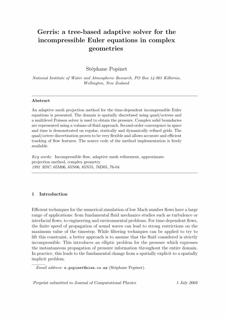
the origin and of radius 1/4. The resulting discretisation for L = 6 is illustrated infigure 9. The same simple problem is then solved on this mesh. Figure 10 gives theconvergence rate of the residual for a mesh with L = 7. The residual reduction factoris about 15 per V-cycle. The order of the solver for the same problem is illustrated infigure 11. Close to second-order convergence in all norms is obtained which confirmsthat the gradient operator described previously is second-order accurate at coarse/finemesh boundaries.

In order to test the ability of the method in presence of solid boundaries, we set upa series of tests with a variety of solid geometries. The corresponding solutions of thePoisson equation are illustrated in figure 12. All problems use the source term definedby (14) where x and y are the coordinates of the geometric centre of the cell considered[23] . A circular solid boundary centred on the origin and of radius 1/4 is used for (a).A star-shaped solid boundary defined in polar coordinates as

r(θ) = 0.237 + 0.079 cos(6θ),

14

0 2 4 6 8 10V-cycle

10-10

10-8

10-6

10-4

10-2

100

102

104

PSfrag replacements

‖aR‖ ∞

0 2 4 6 8 10V-cycle

0

10

20

30

40

50

Res

idua

l red

uctio

n fa

ctor

(a) (b)

Fig. 10. Speed of convergence of the Poisson solver for a simple problem discretised using amesh similar to figure 9 with L = 7. (a) Evolution of the residual. (b) Reduction factor.

5 6 7 8 9 1010-5

10-4

10-3

10-2

10-1

100

Err

or n

orm

s

PSfrag replacements

L

‖ae‖1

‖ae‖2

‖ae‖∞

6 7 8 9 100

1

2

3

Ord

er

PSfrag replacements

L

O1

O2

O∞

(a) (b)

Fig. 11. Order of convergence of the Poisson solver for a simple problem discretised using amesh similar to figure 9. (a) Evolution of the error and (b) order of convergence as functionsof resolution.

is used in problem (b) and an ellipse centred on the origin measuring 34× 5

8in problem

(c). All problems use Neumann conditions on all boundaries. Figure 13 illustrates theconvergence speed for the three problems with L = 7 levels of refinement. The “star”problem (b) is notably more difficult to solve with an average reduction factor of onlyfive per V-cycle. This is due to the limitation of the volume-of-fluid representation ofthe solid boundaries. As mentioned earlier, the features of the solid boundaries areonly represented accurately if their spatial scale is comparable to the mesh size. Forthe “star” problem, while the geometry is represented correctly on the finest level, itis not well represented on all the coarser levels used by the multigrid procedure. Cases(a) and (b) do not have this problem because the smallest spatial scales of the solidboundaries (circle and ellipse) are comparable to the domain size.

The evolution of the error with resolution and the associated convergence order is givenin figure 14. As the exact solution of the problem is not known analytically, Richardson

15

(a) (b) (c)

Fig. 12. Contour plots of the solution of Poisson problems with solid boundaries.

0 2 4 6 8 10V-cycle

0

10

20

30

Res

idua

l red

uctio

n fa

ctor

0 2 4 6 8 10V-cycle

0

10

20

30R

esid

ual r

educ

tion

fact

or

0 2 4 6 8 10V-cycle

0

10

20

30

Res

idua

l red

uctio

n fa

ctor

(a) (b) (c)

Fig. 13. Residual reduction factor for Poisson problems with solid boundaries, L = 7.

3 4 5 6 7 810-5

10-4

10-3

10-2

10-1

100

Err

or n

orm

s

PSfrag replacements

L

‖ae‖1‖ae‖2‖ae‖∞

3 4 5 6 7 810-5

10-4

10-3

10-2

10-1

100

Err

or n

orm

s

PSfrag replacements

L

‖ae‖1‖ae‖2‖ae‖∞

3 4 5 6 7 810-5

10-4

10-3

10-2

10-1

100

Err

or n

orm

s

PSfrag replacements

L

‖ae‖1‖ae‖2‖ae‖∞

3 4 5 6 7 80

1

2

3

Ord

er

PSfrag replacements

L

O1O2

O∞

O∞ (average)3 4 5 6 7 8

0

1

2

3

Ord

er

PSfrag replacements

L

O1O2

O∞

O∞ (average)3 4 5 6 7 8

0

1

2

3

Ord

er

PSfrag replacements

L

O1O2

O∞

O∞ (average)

(a) (b) (c)

Fig. 14. Evolution of the error and associated convergence order for Poisson problems withsolid boundaries.

extrapolation is used. That is, the error for a given level of refinement L is computedby taking the solution at level L+ 1 as reference.

16

Fig. 15. Boundary-refined mesh for problem 12.b, L = 6.

0 2 4 6 8 10V-cycle

0

10

20

30

Res

idua

l red

uctio

n fa

ctor

0 2 4 6 8 10V-cycle

0

10

20

30

Res

idua

l red

uctio

n fa

ctor

0 2 4 6 8 10V-cycle

0

10

20

30

Res

idua

l red

uctio

n fa

ctor

(a) (b) (c)

Fig. 16. Residual reduction factor for Poisson problems with refined solid boundaries, L = 7.

A combination of solid boundaries and refinement is tested using a discretisation withL− 2 levels of refinement on the whole domain plus two levels added only in cells cutby the solid boundary (a discretisation example is given in figure 15 for problem 12.band L = 6). Figures 16 and 17 illustrate the convergence speed and the order of themethod using this discretisation.

The convergence is close to second-order (asymptotically in L) for all norms in allcases. The second-order convergence of the maximum error ‖ae‖∞ is surprising asthe discretisation of the pressure gradient fluxes is only first-order accurate near solidboundaries (as described in section 4). This first-order error in the pressure gradientfluxes should lead to an O(1) truncation error of the Laplacian operator. Johansenand Colella [23] have demonstrated that a scheme with an O(1) truncation error willlead to an O(h) error on the solution for the pressure, in contradiction to the O(h2)convergence we obtain here.

To try to clarify this issue we present truncation and solution errors for the test case

17

5 6 7 8 9 1010-5

10-4

10-3

10-2

10-1

100

Err

or n

orm

s

PSfrag replacements

L

‖ae‖1‖ae‖2‖ae‖∞

5 6 7 8 9 1010-5

10-4

10-3

10-2

10-1

100

Err

or n

orm

s

PSfrag replacements

L

‖ae‖1‖ae‖2‖ae‖∞

5 6 7 8 9 1010-5

10-4

10-3

10-2

10-1

100

Err

or n

orm

s

PSfrag replacements

L

‖ae‖1‖ae‖2‖ae‖∞

5 6 7 8 9 100

1

2

3

Ord

er

PSfrag replacements

L

O1O2O∞

O∞ (average)5 6 7 8 9 10

0

1

2

3

Ord

erPSfrag replacements

L

O1O2O∞

O∞ (average)5 6 7 8 9 10

0

1

2

3

Ord

er

PSfrag replacements

L

O1O2O∞

O∞ (average)

(a) (b) (c)

Fig. 17. Evolution of the error and associated convergence order for Poisson problems withrefined solid boundaries.

used in [23,24]. The embedded boundary is defined by the curve,

r(θ) = 0.30 + 0.15 cos 6θ.

The divergence is set in each full cell as

∇ ·U??(r, θ) = 7r2 cos 3θ.

The exaction solution for this system is φ(r, θ) = r4 cos 3θ. A mesh similar to figure 15is used, with two levels of refinement added near the embedded boundary. In mixedcells, in order to be able to use Neumann boundary conditions at the solid surface whileretaining the exact solution, the flux of the gradient of the exact solution through theboundary is subtracted from the divergence, giving

∇ ·U??(r, θ) = 7r2 cos 3θ − s(nx∇xφ+ ny∇yφ)

ah,

where s is the length of the embedded boundary contained within the cell, nx and ny

are the components of the outward-pointing unit normal to the solid boundary. Thegradients of the exact solution are defined as

∇xφ=4x4 − 3x2y2 − 3y4

r, (16)

∇yφ=xy (5x2 + 9y2)

r, (17)

where x and y are the coordinates of the center of mass of the piece of embeddedboundary contained within the cell.

18

7 8 9 10 1110-7

10-6

10-5

10-4

10-3

Err

or n

orm

s

PSfrag replacements

L

‖ae‖1

‖ae‖2

‖ae‖∞

7 8 9 10 1110-3

10-2

10-1

100

Err

or n

orm

s

PSfrag replacements

L

‖aτ‖1

‖aτ‖2

‖aτ‖∞

7 8 9 10 110

1

2

3

Ord

er

PSfrag replacements

L

O1

O2

O∞

O∞ (average)7 8 9 10 11

0

1

2

3

Ord

erPSfrag replacements

L

O1

O2

O∞

O∞ (average)

(a) (b)

Fig. 18. Evolution of the error and associated convergence order for the Neumann Pois-son problem of [23,24] using locally refined solid boundaries. (a) Error on the solution. (b)Volume-weighted truncation error on the Laplacian of the exact solution.

The results are summarized in figure 18. Figure 18.(a) gives the error norms and cor-responding orders of convergence of the computed solution as functions of the levelof refinement L. Figure 18.(b) illustrates the volume-weighted truncation error of thenumerical Laplacian L defined in section 4.1. As expected the max-norm of the trun-cation error of the numerical Laplacian is O(1) due to the O(h) error in the pressuregradient fluxes in mixed cells, while the orders of the 1- and 2-norm are close to oneand one-half respectively. However, while one would expect only first order convergenceof the max-norm of the error on the solution, second-order convergence in all norms isobtained as illustrated in figure 18.(a). This confirms the results obtained for the pre-vious tests and implies that second-order convergence in all norms can be obtained forpractical problems even if the truncation error on the Laplacian is O(1). The discrep-ancy between our results and the theoretical study of Johansen and Colella could beexplained if second-order converging errors in the bulk of the flow were always largerthan first-order converging errors in mixed cells for all the tests we performed. Thisseems unlikely but if this were the case, it would be necessary to find more stringenttest cases than used in this study or in [23,24]. Further work in this direction wouldbe useful.

Finally, figure 19 shows how the solver scales with problem size. Problem 12.a wassolved on successively finer grids and the average residual reduction factor was com-

19

2 4 6 8 108

10

12

14

16

Res

idua

l red

uctio

n fa

ctor

PSfrag replacements

L

Fig. 19. Average residual reduction factor for problem 12.a as a function of resolution L.

puted as(‖aR0‖∞‖aRn‖∞

) 1n

,

where Ri is the residual after i V-cycle have been applied and n is the total numberof V-cycles (10 in this test). The residual reduction factor decreases approximatelylinearly with resolution level L. The computational cost of solving a problem with22L = N2 degrees of freedom (in 2D) thus scales as O(N 2 logN) as expected from amultigrid scheme.

5 Advection term

We use a conservative formulation for the evaluation of the advection term. Given acell C of boundary ∂C, using the divergence theorem and the non-divergence of thevelocity field, the finite volume advection term An+1/2 of (1) can be computed as

∫

C

An+1/2 =∫

C

[(U · ∇)U]n+1/2 =∫

C

[∇ · (UU)]n+1/2 =∫

∂C

Un+1/2(Un+1/2 · n),

where n is the outward unit normal of ∂C. In the case of our cubic discretisation cellthis can be written

ahAn+1/2 =∑

d

sdUn+1/2

d un+1/2

d , (18)

where Un+1/2

d is the velocity at the centre of the face in direction d at time n+1/2 and

un+1/2

d is the normal component of the velocity at the centre of the face in directiond at time n + 1/2. In order to compute these time- and face-centred values, we use aGodunov procedure [5] i.e. the leading terms of a Taylor series of the velocity of the

20

form

Un+1/2

d = Un +h

2∂dU

n +∆t

2∂tU

n +O(h2,∆t2

),

where ∂d designates the spatial derivative in direction d. Using the Euler equations,the temporal derivative can be replaced by spatial derivatives yielding

Un+1/2

d = Un +

[h

2− ∆t

2vn

d

]∂dU

n − ∆t

2vn⊥d∂⊥dU

n − ∆t

2∇pn,

where ⊥d is the direction perpendicular to d in 2D (in 3D the sum over the twoperpendicular directions) and vd is the velocity component in direction d at the centre

of the cell. Given a cell face, two values of Un+1/2

d can be constructed, one for each cellsharing this face. In the original Godunov method for compressible fluids an uniquevalue is constructed from these two values by solving a Riemann problem. In theincompressible case, simple upwinding is sufficient [5].

Following [21,22] we use a simplified upwind scheme of the form

Un+1/2

d (C) = Un +h

2min

(1− vn

d

∆t

h, 1)∂dU

n − ∆t

2vn⊥d∂⊥dU

n (19)

where ∂⊥dUn is the upwinded derivative in direction ⊥d

∂⊥dUn =

∇⊥dU

n if vn⊥d < 0

∇⊥d

Un if vn⊥d > 0

(20)

∇⊥d is computed as in section 4.1 and ⊥d is the direction opposite to ⊥d. The cell-centred derivative ∂dU

n is computed by fitting a parabola through the centre of C andof its neighbours in directions d and d. If the neighbours are on different levels, aninterpolation or averaging procedure similar to that presented in section 4.1 is used. Inthe case of neighbouring cells at the same level, this procedure reduces to the classicalsecond-order accurate centred difference scheme. We also do not use any slope limiterson the derivatives as we do not expect strong discontinuities in the velocity field forincompressible flows. Slope limiters can easily be added in this scheme if necessary.

Given the time- and face-centred values Un+1/2

d (C) and Un+1/2

d(Nd) we then choose the

upwind state

Un+1/2

d (C) = Un+1/2

d(Nd) =

Un+1/2

d (C) if und > 0

Un+1/2

d(Nd) if un

d < 0

12(U

n+1/2

d (C) + Un+1/2

d(Nd)) if un

d = 0

(21)

where Nd is the neighbour of C in direction d. If Nd is at a lower level (figure 20)and un

d ≤ 0, the value upwinded from Nd at the centre of the face (marked by )

21

PSfrag replacements

C

Nd

N⊥d

Ud

Ud

Ud U

U ud

Cd

Fig. 20. Upwinding in the case of neighbouring cells at different levels. Linear interpolationis used to derive the value on the right side of Cd.

is interpolated linearly from Un+1/2

d(Nd) and from the value for its neighbour (or its

children) in the correct direction, Un+1/2

d(N⊥d).

In order to compute the advection term using (18), we first need to construct the face-

and time-centred normal velocities un+1/2

d . If we want the method to be conservative,these normal velocities have to be discretely divergence-free. In a first step, normalvelocities are constructed for both sides of each cell face using (19) and (20) where vn

d

and vn⊥d are the corresponding components of the centred velocity Un. The upwind

state u?d is then selected for each face using (21) where un

d is obtained by linear inter-polation of the relevant component of the centred velocities Un(C) and Un(Nd). Tomake this set of normal velocities divergence-free we then apply a projection step bysolving

L(φ) = ∇ · u?, (22)

where ∇ · u? is the finite-volume divergence of the normal velocity field, expressed foreach cell as

∇ · u? =1

ah

∑

d

sdu?d. (23)

By correcting u? with the pressure solution, we obtain a set of face- and time-centrednormal velocities

un+1/2

d = u?d −∇dφ. (24)

22

When correcting the normal velocities, we also calculate a cell-centred value for thepressure gradient by simple averaging of face gradients

∇?dφ =

∇dφ−∇dφ

2. (25)

To compute the advection term An+1/2, we first need to re-predict the face-centredvelocities U

n+1/2

d , this time using un+1/2

d rather than averages from cell-centred values.Again, in a first step, normal velocities are constructed for both sides of each cell faceusing (19) and (20) where we now take vn

d = (un+1/2

d − un+1/2

d)/2. A unique value

U?d is then selected for each face using (21). A face-centred pressure gradient ∇φ is

then computed by linear interpolation from the average cell-centred values ∇?φ(C) and∇?φ(Nd) (or its children). The predicted value is then obtained as

Un+1/2

d = U?d − ∇φ.

Note that we could re-use the face- and time-centred normal velocities un+1/2

d as pre-dicted values (the tangential component would still need to be recalculated), however,we have found this approach to be unstable for flow around sharp angles. The spatialfiltering of the pressure gradient provided by the averaging procedure seems to benecessary to ensure stability in this particular case.

5.1 Small-cell problem

To obtain the provisional cell-centred velocity field U?? using (1), it is necessary todivide the finite volume advection term (18) by the volume of the cell (ah2) to getAn+1/2. This leads to the classical CFL stability condition

‖U‖∆tah

≤ 1,

which expresses the condition that a cell should not “overflow” during a given timestep.In the general case, the fluid fraction a can be arbitrarily small with a correspondingrestrictive condition on the maximum timestep. This is traditionally referred to as the“small-cell problem”. A number of approaches exist to work around this problem: cellmerging [37,14], redistribution [15] or special difference schemes [13]. We have chosento use a simple cell-merging technique similar to that presented by Quirk [14]. Atinitialisation time, after the volume and area fractions have been computed, all smallcells are assigned a pointer to their biggest neighbour B (as measured by the fluidfraction a). For a given timestep, the advection term ah2An+1/2 is then computed inall cells as described above. To compute the advection update to the velocity, smallcells are first grouped with adjacent mixed or full cells using the following recursivealgorithm:

23

Group (G, C)if C does not already belong to any group then

Add C to Gif C is a small cell then

Group (G, B(C))end iffor each direction d

if Nd is a small cell thenGroup (G, Nd)

end ifend for

end if

where G is the resulting group of cells. For each group, the weighted averaged updateis computed as

An+1/2

G =

∑G ah

2An+1/2

∑G ah2

.

Each cell in the group then receives a fraction of the update proportional to its volume

An+1/2 ≈ ah2

∑G ah2

An+1/2

G .

This is equivalent to using a “virtual” cell formed by all the cells in the group. The CFLstability now depends on the total volume of the group of cells. In practice, choosingto define small cells as cells for which a < 1/2 ensured stability in all the cases wetested.

6 Approximate projection

While it is easy to formulate an exact projection operator for MAC (staggered, face-based) discretisation of the velocity field, it is difficult to do the same for a cell-centreddiscretisation. This is due to the spatial decoupling of the stencils used for the relax-ation operator. This can cause numerical instabilities in the pressure field and makesefficient implementation of multigrid techniques difficult [38,9]. Attempts to coupleneighbouring pressure cells through asymmetric operators have been unsuccessful [39].

Drawing from these conclusions, Almgren, Bell and Szymczak [12] dropped the re-quirement of exact discrete non-divergence of the projected cell-centred velocity fieldand proposed to use an approximate Laplacian operator well-behaved with respect tospatial coupling. Following Lai [38], Minion [11] and Martin [21] we use an approximateprojection based on face-centred interpolation of the cell-centred velocity field. In afirst step, face-centred normal components of the velocity are constructed by interpo-lation of the cell-centred provisional velocity U??. This normal (MAC) velocity field is

24

then projected using the exact projection operator (following steps (22) to (24)) andaverage cell-centred pressure gradients are constructed (using (25)). These pressuregradients are then used to correct U?? to obtain the approximately divergence-freevelocity field Un+1.

A detailed study of the stability of the approximate projection can be found in [40,41].The use of pressure filters was found to be necessary in some cases (long, quasi-stationary simulations) to avoid a gradual build-up of non-divergence-free velocitymodes. We do not use pressure filters in the current version of the code but did notencounter any noticeable numerical instabilities for the various tests we performed.

It is also important to note that even if the resulting cell-centred velocity field isnot exactly divergence-free, the face-centred normal advection field u

n+1/2

d is exactlydiscretely divergence-free, so that the advection scheme is exactly conservative. Thisis particularly important for the treatment of variable density flows.

7 Adaptive mesh refinement

Using a tree-based discretisation, it is relatively simple to implement a fully flexibleadaptive refinement strategy.

In a first step, all the leaf cells which satisfy a given criterion are refined (as well astheir neighbours when necessary, in order to respect the constraints described in figure2). This step could be repeated recursively but we generally assume that the flow isevolving slowly (compared to the frequency of adaptation) so that only one pass isnecessary.

In a second step, we consider the parent cells of all the leaf cells (i.e. the immediatelycoarser discretisation). All of these cells which do not satisfy the refinement criterionare coarsened (i.e. become leaf cells).

The values of the cell-centred variables for newly created or coarsened cells must beinitialised. For newly coarsened cells, it is consistent to compute these values as the vol-ume weighted average of the values of their (defunct) children, so that quantities suchas momentum are preserved exactly. For newly created cells, the solution is less obvi-ous. In particular, it is desirable that momentum and vorticity are locally preserved.Unfortunately, this is not simple to achieve in practice. We have chosen a simple linearinterpolation procedure using the parent cell value and its gradients. Given a newlycreated cell C with parent cell P , the new cell-centred value v(C) is obtained as

v(C) = v(P) + ∆x∇xv(P) + ∆y∇yv(P),

where (∆x,∆y) are the coordinates of the centre of C relative to the centre of P . Thisformula guarantees local conservation of momentum but tends to introduce numerical

25

noise in the vorticity field. A better choice may be higher-order interpolants such asbicubic interpolation.

On the new discretisation, there is no guarantee that the velocity field is divergence-free anymore. A projection step is then needed. To avoid the cost of an extra projectionstep when adapting the grid, we perform the grid refinement at the fractional timestep,using the provisional velocity field U??, just before the approximate projection is ap-plied.

Various choices are possible for the refinement criterion. An attractive option would beto use Richardson extrapolation to obtain a numerical approximation of the truncationerror of the whole scheme [42,21]. For the moment, we use a simple criterion based onthe norm of the local vorticity vector. Specifically, a cell is refined whenever

h‖∇ ×U‖max ‖U‖ > τ,

where max ‖U‖ is evaluated over the entire domain. The threshold value τ can be in-terpreted as the maximum acceptable angular deviation (caused by the local vorticity)of a particle travelling at speed max ‖U‖ across the cell.

The computational cost of this algorithm is small compared to the cost of the Poissonsolver. It can be applied at every timestep with a negligible overall penalty (less than5% of the total cost).

8 Numerical results

Following Minion [11] and Almgren et al. [43], we present two convergence tests illus-trating the second-order accuracy of our method for flows without solid boundaries.The first problem uses a square unit domain with periodic boundary conditions inboth directions. The initial conditions are taken as

u(x, y) = 1− 2 cos(2πx) sin(2πy),

v(x, y) = 1 + 2 sin(2πx) cos(2πy).

The exact solution of the Euler equations for these initial conditions is

u(x, y, t) = 1− 2 cos(2π(x− t)) sin(2π(y − t)),v(x, y, t) = 1 + 2 sin(2π(x− t)) cos(2π(y − t)),p(x, y, t) =− cos(4π(x− t))− cos(4π(y − t)).

As in [43] nine runs are performed on grids with L = 5, 6 and 7 levels of refinement(labelled “uniform”) and with one (labelled r = 1) or two (labelled r = 2) additional

26

Patch L2

L = 5 O2 L = 6 O2 L = 7

r = 1 6.80e-3 2.19 1.49e-3 2.05 3.61e-4

r = 2 4.91e-3 1.66 1.55e-3 1.81 4.39e-4

Domain L2

L = 5 O2 L = 6 O2 L = 7

Uniform 7.70e-3 2.87 1.05e-3 2.65 1.67e-4

r = 1 9.52e-3 2.39 1.81e-3 2.17 4.01e-4

r = 2 1.22e-2 2.19 2.67e-3 2.09 6.29e-4

Patch L∞

L = 5 O∞ L = 6 O∞ L = 7

r = 1 1.73e-2 1.82 4.89e-3 1.91 1.30e-3

r = 2 1.58e-2 1.41 5.96e-3 1.84 1.66e-3

Domain L∞

L = 5 O∞ L = 6 O∞ L = 7

Uniform 1.74e-2 2.62 2.84e-3 2.68 4.44e-4

r = 1 2.27e-2 2.14 5.15e-3 1.93 1.35e-3

r = 2 2.76e-2 2.21 5.96e-3 1.84 1.66e-3

Table 1Errors and convergence orders in the x-component of the velocity for a simple periodicproblem.

levels added only within the square defined by the points (−0.25,−0.25) and (0, 0).The length of the run for each case is 0.5, the CFL number is 0.75. For each run boththe L2 and L∞ norms of the error in the x-component of the velocity is computedusing (12) for both the whole domain (labelled “domain”) and the refined region only(labelled “patch”). Table 1 gives the errors and order of convergence obtained.

Close to second-order convergence is obtained (asymptotically in L) for the L2 andL∞ norms on both uniform and refined domains. The values obtained are comparableto that in [11,43]. The error in the refined patch is comparable to the error at theresolution of the base grid. This is expected, given the arbitrary placement of therefined patch, the error is controlled mainly by the surrounding coarse cells.

The second test is the four-way vortex merging problem of Almgren et al. [43]. Itdemonstrates the convergence of the method when refinement is placed appropriately.

Four vortices are placed in the unit-square, centred at (0, 0), (0.09, 0), (−0.045, 0.045√

3)

27

and (−0.045, −0.045√

3) and of strengths −150, 50, 50, 50 respectively. The profile ofeach vortex centred around (xi, yi) is

1 + tanh(100(0.03− ri))

2,

where ri =√

(x− xi)2 + (y − yi)2. To initialise the velocity field, we use this vorticityas the source term in the Poisson equation for the streamfunction ψ

∇2ψ = ‖∇ ×U‖.

Each component of the velocity field is then calculated from the streamfunction. No-flow boundary conditions are used on the four sides of the domain and the simulationsare ran to t = 0.25 using a CFL of 0.9.

Five different discretisations are used, each time with up to L levels of refinement: auniform grid, a grid using static refinement in concentric circles of decreasing radius andthe dynamic adaptive refinement described in section 7. The “circle” grid is constructedby starting from a uniform grid with four levels of refinement and by successivelyadding one level to all the cells contained within circles centred on the origin and ofradii:

• L = 6: 0.25, 0.15• L = 7: 0.25, 0.2, 0.15• L = 8: 0.25, 0.2, 0.175, 0.15• L = 9: 0.25, 0.2, 0.175, 0.1625, 0.15• L = 10: 0.25, 0.225, 0.2, 0.175, 0.1625, 0.15

For the dynamically refined grid, the vorticity-based criterion is applied at everytimestep with a threshold τ = 4 × 10−3. As we do not have an analytical solutionfor this problem, Richardson extrapolation is used.

Figure 21 illustrates the evolution of the vorticity and of the adaptively refined grid forL = 8. The most refined level closely follows the three outer vortices as they orbit thecentral one. Far from the vortices, a very coarse mesh is used (l = 3). One may note afew isolated patches of refinement scattered at the periphery of the outer vortices. Theyare due to the numerical noise added to the vorticity by the interpolation procedurenecessary to fill in velocity values for newly created cells. As mentioned in section7, this could be improved by using higher-order interpolants. This numerical noise issmall enough that it does not compromise the convergence properties of the adaptivemethod (as shown below).

Table 2 summarises the results obtained for the first twelve calculations. For fineenough grids close to second-order convergence is obtained for both norms and forthe three discretisations used. The norms of the error on the various grids are alsocomparable for a given resolution.

Table 3 gives the CPU time and the size of the problems solved for all three grids

28

Domain L2

L = 6 O2 L = 7 O2 L = 8 O2 L = 9

Uniform 2.61e-2 1.31 1.05e-2 1.97 2.68e-3 2.11 6.19e-4

Circle 2.61e-2 1.33 1.04e-2 1.96 2.68e-3 1.98 6.81e-4

Adaptive 2.66e-2 1.35 1.04e-2 2.07 2.47e-3 2.05 5.96e-4

Domain L∞

L = 6 O∞ L = 7 O∞ L = 8 O∞ L = 9

Uniform 4.46e-1 1.25 1.87e-1 1.95 4.84e-2 1.85 1.34e-2

Circle 4.49e-1 1.27 1.86e-1 1.94 4.85e-2 1.87 1.33e-2

Adaptive 4.45e-1 1.26 1.86e-1 1.94 4.86e-2 1.83 1.37e-2

Table 2Errors and convergence orders in the x-component of the velocity for the four-way vortexmerging problem.

CPU Time Cells advanced

Total (s) µs/cell Number

Uniform L = 8 1486 167 8,912,896

Circle L = 8 166 222 746,368

Adaptive L = 8 117 286 409,632

Uniform L = 9 13,034 166 78,643,200

Circle L = 9 1024 183 5,608,960

Adaptive L = 9 764 326 2,342,200

Table 3Timings for uniform, circle and adaptive grids for the four-way vortex merging problem.

and for two levels of refinement. A PC-compatible Pentium 350 MHz machine wasused. The total number of leaf cells advanced for the whole calculation is given as wellas the corresponding average speed. For L = 8, a speedup of about nine is obtainedwhen using the statically refined “circle” grid, and thirteen when using the adaptivetechnique. Both the “circle” and adaptive discretisations are notably slower (per cell)than the uniform discretisation. This is mainly due to the interpolations necessary tocompute the pressure gradient at coarse/fine cell boundaries when solving the Poissonequation (figure 4). It is also interesting to note that the CPU times obtained are veryclose to those reported by Almgren et al. [43] for the same problem (keeping in mindthat they used a Cartesian AMR technique on a DEC Alpha computer and solved aviscous flow).

To demonstrate the convergence properties of the method in the presence of solidboundaries, we use a test case initially presented by Almgren et al. [15]. A diverging

29

t = 0.05

t = 0.15

t = 0.25

Fig. 21. Contour plots of vorticity (left) and adaptive grids used (right) for the four-wayvortex merging calculation. The lines on the pictures in the right column represent theboundaries between levels of refinement (with a maximum of L = 8 levels).

channel is constructed in a 4×1 domain by restricting the fluid flow through the curves

30

All cells Full level 5 cells

5–6 Rate 6–7 5–6 Rate 6–7

L1 2.66e-4 1.81 7.60e-5 2.41e-4 1.85 6.69e-5

L2 5.83e-4 1.44 2.15e-4 5.36e-4 1.49 1.91e-4

L∞ 5.05e-3 0.89 2.72e-3 3.77e-3 0.93 1.98e-3

Table 4Errors and convergence rates for the x-component of the velocity.

All cells Full level 5 cells

5–6 Rate 6–7 5–6 Rate 6–7

L1 2.75e-4 1.95 7.11e-5 2.31e-4 2.16 5.17e-5

L2 7.09e-4 1.32 2.84e-4 6.76e-4 1.59 2.25e-4

L∞ 7.47e-3 1.05 3.60e-3 5.98e-3 1.07 2.85e-3

Table 5Errors and convergence rates for the y-component of the velocity.

ytop and ybot, defined as

ybot =

y1 if 0 ≤ x ≤ 1

y2 + 0.5(y1 − y2)(1 + cos(π2(x− 1)) if 1 < x < 3

y2 if 3 ≤ x ≤ 4

andytop = 1− ybot,

with y1 = 0.2 and y2 = 10−6. Neumann boundary conditions for the pressure are setat the inlet (x = 0) and at the solid boundaries. A fixed unity inflow velocity is setat the inlet and simple outflow boundary conditions at the outlet (the pressure andthe gradients of all the components of the velocity are set to zero at x = 4). Thesimulations are ran to t = 1 using a CFL of 0.8. Three simulations are performedon uniform grids with L = 5, 6 and 7 levels of refinement. Table 4 and 5 show theerrors and convergence rates obtained. As in [15] we calculate errors both on thefull domain (“All cells”) and on the part of the domain covered by cells at level 5entirely contained within the fluid (“Full level 5 cells”). Columns labelled “5–6” givethe error computed on the mesh with 5 levels of refinement using the mesh with 6levels of refinement as reference (and similarly for columns labelled “6–7”). For bothcomponents of the velocity close to first-order convergence is obtained for the L∞ normand close to second-order convergence for the L1 norm, as expected from a solutionglobally second-order accurate but first-order accurate at the boundaries. Figure 22confirms that the error is concentrated near solid boundaries. The maximum error ineither component is small (less than one percent of the magnitude of the velocity).

Finally, we present an application of the three-dimensional version of the code to a

31

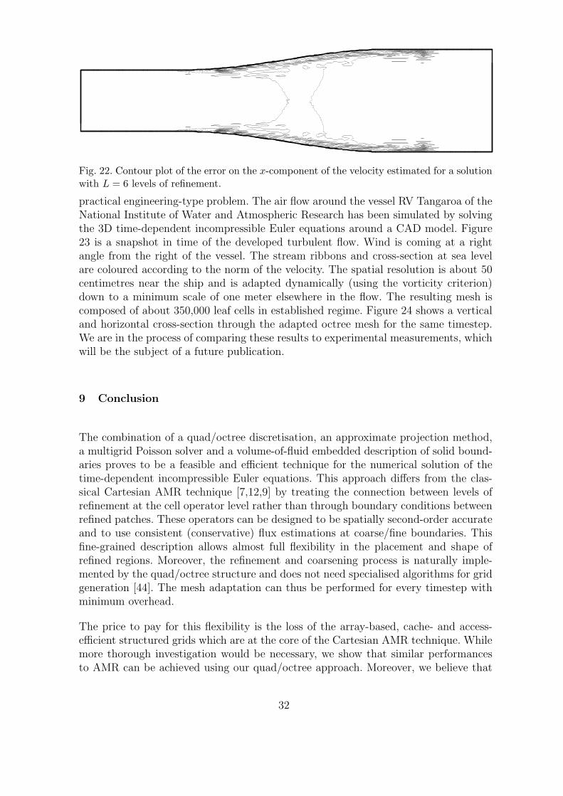
Fig. 22. Contour plot of the error on the x-component of the velocity estimated for a solutionwith L = 6 levels of refinement.

practical engineering-type problem. The air flow around the vessel RV Tangaroa of theNational Institute of Water and Atmospheric Research has been simulated by solvingthe 3D time-dependent incompressible Euler equations around a CAD model. Figure23 is a snapshot in time of the developed turbulent flow. Wind is coming at a rightangle from the right of the vessel. The stream ribbons and cross-section at sea levelare coloured according to the norm of the velocity. The spatial resolution is about 50centimetres near the ship and is adapted dynamically (using the vorticity criterion)down to a minimum scale of one meter elsewhere in the flow. The resulting mesh iscomposed of about 350,000 leaf cells in established regime. Figure 24 shows a verticaland horizontal cross-section through the adapted octree mesh for the same timestep.We are in the process of comparing these results to experimental measurements, whichwill be the subject of a future publication.

9 Conclusion

The combination of a quad/octree discretisation, an approximate projection method,a multigrid Poisson solver and a volume-of-fluid embedded description of solid bound-aries proves to be a feasible and efficient technique for the numerical solution of thetime-dependent incompressible Euler equations. This approach differs from the clas-sical Cartesian AMR technique [7,12,9] by treating the connection between levels ofrefinement at the cell operator level rather than through boundary conditions betweenrefined patches. These operators can be designed to be spatially second-order accurateand to use consistent (conservative) flux estimations at coarse/fine boundaries. Thisfine-grained description allows almost full flexibility in the placement and shape ofrefined regions. Moreover, the refinement and coarsening process is naturally imple-mented by the quad/octree structure and does not need specialised algorithms for gridgeneration [44]. The mesh adaptation can thus be performed for every timestep withminimum overhead.

The price to pay for this flexibility is the loss of the array-based, cache- and access-efficient structured grids which are at the core of the Cartesian AMR technique. Whilemore thorough investigation would be necessary, we show that similar performancesto AMR can be achieved using our quad/octree approach. Moreover, we believe that

32

in the case of small and complicated structures (such as interfaces between fluids orshocks) the flexibility of this approach can more than compensate for this overhead(given that a Cartesian AMR technique would require a large number of refined patchesto cover the small structures, leading to substantial overheads in boundary conditionsand most probably to the loss of cache-efficiency).

Future developments include extension to the incompressible variable-density Navier–Stokes equations and interfacial flows, using VOF [45] and marker techniques [46].Using sub-cycling in time on different levels of refinement [43] would also be a usefulextension of the algorithm presented.

Finally, by providing an open source version of the code which can be freely redis-tributed and modified [25], we hope to encourage research and collaboration in thisfield.

10 Acknowledgments

This work was funded by the New Zealand Foundation for Research, Science andTechnology and by the Marsden Fund of the Royal Society of New Zealand.

33

References

[1] A. J. Chorin, Numerical solution of the Navier-Stokes equations, Math. Comp. 22 (1968)745–762.

[2] R. Peyret, T. D. Taylor, Computational Methods for Fluid Flow, Springer Verlag, NewYork/Berlin, 1983.

[3] A. Brandt, Guide to multigrid development, Multigrid Methods, Springer Verlag, Berlin,1982.

[4] J. Wesseling, An introduction to Multigrid Methods, Wiley, Chichester, 1992.

[5] J. B. Bell, P. Colella, H. M. Glaz, A second-order projection method for theincompressible Navier-Stokes equations, J. Comput. Phys. 85 (1989) 257–283.

[6] J. B. Bell, D. L. Marcus, A second-order projection method for variable density flows,J. Comput. Phys. 101 (1992) 334–348.

[7] M. J. Berger, J. Oliger, Adaptive mesh refinement for shock hydrodynamics, J. Comput.Phys. 53 (1984) 484–512.

[8] W. J. Coirier, An adaptively-refined, Cartesian, cell-based scheme for the Euler andNavier-Stokes equations, Ph.D. thesis, NASA Lewis Research Center, Cleveland, OH,USA (October 1994).

[9] L. H. Howell, J. B. Bell, An adaptive mesh projection method for viscous incompressibleflow, SIAM Journal on Scientific Computing 18 (4) (1997) 996–1013.

[10] A. M. Khokhlov, Fully threaded tree algorithms for adaptive refinement fluid dynamicssimulations, J. Comput. Phys. 143 (2) (1998) 519–543.

[11] M. L. Minion, A projection method for locally refined grids, J. Comput. Phys. .

[12] A. S. Almgren, J. B. Bell, W. G. Szymczak, A numerical method for the incompressibleNavier-Stokes equations based on an approximate projection, SIAM J. Sci. Comput.17 (2).

[13] M. Berger, R. LeVeque, A rotated difference scheme for Cartesian grids in complexgeometries, in: AIAA 10th Computational Fluid Dynamics Conference, Honolulu,Hawaii, 1991, pp. 1–7.

[14] J. J. Quirk, An alternative to unstructured grids for computing gas dynamics flowsaround arbitrarily complex two-dimensional bodies, Computers and Fluids 23 (1994)125–142.

[15] A. S. Almgren, J. B. Bell, P. Colella, T. Marthaler, A Cartesian grid projection methodfor the incompressible Euler equations in complex geometries, SIAM J. Sci. Comp. 18 (5).

[16] T. Ye, R. Mittal, H. S. Udaykumar, W. Shyy, An accurate cartesian grid method forviscous incompressible flows with complex immersed boundaries, J. Comp. Phys. 156(1999) 209–240.

34

[17] D. Calhoun, R. J. LeVeque, Solving the advection-diffusion equation in irregulargeometries, J. Comp. Phys. 156 (2000) 1–38.

[18] C. S. Peskin, Flow patterns around heart valves: a numerical method, J. Comp. Phys.(1972) 10–252.

[19] E. M. Saiki, S. Biringen, Numerical simulations of a cylinder in a uniform flow:application of a virtual boundary method, J. Comp. Phys. 123 (1996) 450–465.

[20] E. A. Fadlun, R. Verzicco, P. Orlandi, J. Mohd-Yusof, Combined immersed-boundaryfinite-difference methods for three-dimensional complex flow simulations, J. Comp. Phys.161 (2000) 35–60.

[21] D. F. Martin, An adaptive cell-centered projection method for the incompressible Eulerequations, Ph.D. thesis, University of California, Berkeley (1998).

[22] D. F. Martin, P. Colella, A cell-centered adaptive projection method for theincompressible euler equations, J. Comp. Phys. 163 (271-312).

[23] H. Johansen, P. Colella, A cartesian grid embedded boundary method for poisson’sequation on irregular domains, J. Comp. Phys. 147 (1998) 60–85.

[24] M. S. Day, P. Colella, M. J. Lijewski, C. A. Rendleman, D. L. Marcus, Embeddedboundary algorithms for solving the Poisson equation on complex domains, Tech. Rep.LBNL-41811, Lawrence Berkeley National Laboratory (May 1998).

[25] S. Popinet, The Gerris Flow Solver, http://gfs.sourceforge.net.

[26] H. Samet, Applications of Spatial Data Structures, Addison-Wesley PublishingCompany, 1989.

[27] R. Gonzalez, P. Wintz, Digital Image Processing, Addison-Wesley Publishing Company,1987.

[28] M. J. Berger, M. J. Aftosmis, Aspects (and aspect ratios) of Cartesian mesh methods,in: Proceedings of the 16th International Conference on Numerical Methods in FluidDynamics, Springer-Verlag, Arcachon, France, 1998.

[29] L. Balmelli, J. Kovacevic, M. Vetterli, Quadtrees for embedded surface visualization:constraints and efficient data structures, in: Proceedings of IEEE InternationalConference on Image Processing, Vol. 2, 1999, pp. 487–491.

[30] H. Edelsbrunner, E. P. Mucke, Simulation of simplicity: A technique to cope withdegenerate cases in geometric algorithms, ACM Trans. Graph. 9 (1) (1990) 66–104.

[31] K. L. Clarkson, Safe and effective determinant evaluation, in: Proc. 31st IEEESymposium on Foundations of Computer Science, Pittsburgh, PA, 1992, pp. 387–395.

[32] V. J. Milenkovic, Robust polygon modeling, Computer-Aided Design 25 (9) (1993) 546–566.

[33] J. R. Shewchuk, Adaptive precision floating-point arithmetic and fast robust geometricpredicates, Tech. rep., School of Computer Science, Carnegie Mellon University,Pittsburgh, Pennsylvania (May 1996).

35

[34] S. Popinet, The GNU Triangulated Surface Library, http://gts.sourceforge.net.

[35] M. J. Aftosmis, M. J. Berger, J. E. Melton, Robust and efficient Cartesian meshgeneration for component-based geometry, Tech. Rep. AIAA-97-0196, U.S. Air ForceWright Laboratory (1997).

[36] D. L. Brown, R. Cortez, M. L. Minion, Accurate projection methods for theincompressible Navier-Stokes equations, J. Comput. Phys. 168 (2001) 464–499.

[37] W. Noh, Cel: a time-dependent, two-space-dimensional, coupled Eulerian-Lagrangiancode, Fundamental Methods of Hydrodynamics, (Methods of Computational Physics,Volume 3) (1964) 117–179.

[38] M. F. Lai, A projection method for reacting flows in the zero Mach number limit, Ph.D.thesis, University of California at Berkeley (1993).

[39] J. C. Strikwerda, Finite difference methods for the Stokes and Navier-Stokes equations,SIAM J. Sci. Stat. Comput. 5 (1984) 56–67.

[40] W. J. Rider, Approximate projection methods for incompressible flows: Implementation,variants and robustness, Tech. Rep. LA-UR-2000, Los Alamos National Laboratory(1995).

[41] A. S. Almgren, J. B. Bell, W. Y. Crutchfield, Approximate projection methods: Part I.Inviscid analysis, SIAM Journal on Scientific Computing 22 (4) (2000) 1139–1159.

[42] M. J. Berger, P. Colella, Local adaptive mesh refinement for shock hydrodynamics, J.Comput. Phys. 82 (1989) 64–84.

[43] A. S. Almgren, J. B. Bell, P. Colella, L. H. Howell, M. L. Welcome, A conservativeadaptive projection method for the variable density incompressible Navier-Stokesequations, J. Comp. Phys. 142 (1998) 1–46.

[44] M. J. Berger, I. Rigoutsos, An algorithm for point clustering and grid generation, IEEETrans. Systems, Man and Cybernet 21 (1991) 1278–1286.

[45] D. Gueyffier, A. Nadim, J. Li, R. Scardovelli, S. Zaleski, Volume of fluid interface trackingwith smoothed surface stress methods for three-dimensional flows, J. Comp. Phys. 152(1998) 423–456.

[46] S. Popinet, S. Zaleski, A front tracking algorithm for the accurate representation ofsurface tension, Int. J. Numer. Meth. Fluids 30 (1999) 775–793.

36

Fig. 23. Airflow around RV Tangaroa. The stream ribbons and cross-section at sea level arecoloured according to the norm of the velocity.

Fig. 24. Adaptive mesh. The horizontal and vertical cross-sections illustrate thethree-dimensional adaptive octree.

37