german openfoam user meeting 2017 (gofun 2017 ... · pdf filegerman openfoam user meeting 2017...

LeMoS

German OpenFOAM User meeting 2017 (GOFUN 2017)

Particle Simulation withOpenFOAM®

Introduction, Fundamentals andApplications

ROBERT KASPERChair of Modeling and Simulation,University of Rostock

March 21, 2017 © 2017 UNIVERSITY OF ROSTOCK | CHAIR OF MODELING AND SIMULATION 1 / 44

LeMoS

Outline

IntroductionMotivationLagrangian-Particle-Tracking in OpenFOAM

Fundamentals of Lagrangian-Particle-TrackingGoverning EquationsParticle ForcesParticle Response TimePhase-Coupling MechanismsParticle-Particle Interaction

ApplicationHow to build your own Eulerian-Lagrangian Solver in OpenFOAMHow to use your own Eulerian-Lagrangian Solver in OpenFOAMPost-Processing with OpenFOAM/Paraview


LeMoS

Outline





LeMoS

Why Particle Simulations with OpenFOAM?

• OpenFOAM is free and open source(customization and unlimited parallelizationpossible)

• OpenFOAM is constantly under developmentwith a continuous growing community(academic research, R&D in companies)

• OpenFOAM includes solvers for anyapplication of particle-laden flows (e.g.process engineering, mechanicalengineering, civil engineering, physics,...)


LeMoS

Lagrangian-Particle-Tracking in OpenFOAM

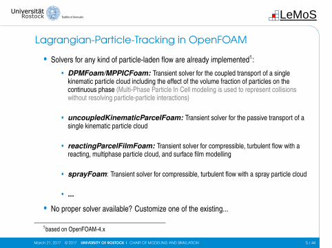
• Solvers for any kind of particle-laden flow are already implemented1:

• DPMFoam/MPPICFoam: Transient solver for the coupled transport of a singlekinematic particle cloud including the effect of the volume fraction of particles on thecontinuous phase (Multi-Phase Particle In Cell modeling is used to represent collisionswithout resolving particle-particle interactions)

• uncoupledKinematicParcelFoam: Transient solver for the passive transport of asingle kinematic particle cloud

• reactingParcelFilmFoam: Transient solver for compressible, turbulent flow with areacting, multiphase particle cloud, and surface film modelling

• sprayFoam: Transient solver for compressible, turbulent flow with a spray particle cloud

• ...

• No proper solver available? Customize one of the existing...

1based on OpenFOAM-4.x


LeMoS

Outline





LeMoS

Governing Equations of Lagrangian-Particle-Tracking

• Calculation of isothermal particle motions requires the solution of the following set ofordinary differential equations:

dxpdt

= up, mpdup

dt=∑

Fi, Ipdωp

dt=∑

T (1)

• Newton’s second law of motion presupposes the consideration of all relevant forcesacting on the particle, e.g., drag, gravitational and buoyancy forces, pressure forces:

mpdup

dt=∑

Fi = FD + FG + FP + ... (2)


LeMoS

Drag Force

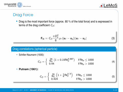
• Drag is the most important force (approx. 80 % of the total force) and is expressed interms of the drag coefficient CD :

FD = CDπD2

p

8ρf (uf − up) |uf − up| (3)

Drag correlations (spherical particle)

• Schiller-Naumann (1935):

CD =

{ 24Rep

(1 + 0.15Re0.687

p

)if Rep ≤ 1000

0.44 if Rep > 1000(4)

• Putnam (1961):

CD =

{24Rep

(1 + 1

6 Re2/3p

)if Rep ≤ 1000

0.424 if Rep > 1000(5)


LeMoS

Drag Force

10−1 100 101 102 103 104 105 106

10−1

100

101

102

Rep =ρfDp|uf−up|

µf[-]

CD

[-]

MeasurementStokes regimeNewton regimeSchiller-NaumannPutnam

Figure: Drag coefficient as a function of particle Reynolds number, comparison of experimental data withcorrelations of Schiller-Naumann (1935) and Putnam (1961)


LeMoS

Gravity/Buoyancy and Pressure Gradient Force• Gravitational and Buoyancy force is computed as one total force:

FG = mpg(

1− ρfρp

)(6)

• The force due to a local pressure gradient can be expressed for a spherical particlesimply as:

FP = −πD3

p

6∇p (7)

• Expressing the local pressure gradient∇p in terms of the momentum equation leadsto the final pressure gradient force:

Fp = ρfπD3

p

6

(Duf

Dt−∇ · ν

(∇uf +∇uT

f

))(8)


LeMoS

Other Forces

• Added mass force: particle acceleration or deceleration in a fluid requires also anaccelerating or decelerating of a certain amount of the fluid surrounding the particle(important for liquid-particle flows)

• Slip-shear lift force: particles moving in a shear layer experience a transverse liftforce due to the nonuniform relative velocity over the particle and the resultingnonuniform pressure distribution

• Slip-rotation lift force: particles, which are freely rotating in a flow, may alsoexperience a lift force due to their rotation (Magnus force)

• Thermophoretic force: a thermal force moves fine particles in the direction ofnegative temperature gradients (important for gas-particle flows)

• ...


LeMoS

Particle Response Time• Particle response time is used to characterize the capability of particles to follow

sudden velocity changes in the flow

• Starting from the equation of motion considering only drag force (divided by particlemass and in terms of the particle Reynolds number):

dupdt

=18µfρpD2

p

CD Rep24

(uf − up) →dupdt

=1τp

(uf − up) (9)

Particle response time & Stokes number

τp =ρpD

2p

18µf fD, St = τp/τf (10)

→ The Stokes number St is the ratio of theparticle response time and a characteristictime scale of the flow

Figure: Graphical illustration of the particleresponse time (Sommerfeld, 2011)


LeMoS

Phase-Coupling Mechanisms• Phase-coupling mechanisms strongly influences the behavior of the continous and

dispersed phase:

• One-way coupling: fluid→ particles

• Two-way coupling: fluid � particles

• Four-way coupling: fluid � particles + particle collisions

• Classification of phase-coupling mechanisms according to Elghobashi (1994):

10−8 10−6 10−4 10−2 10010−1

100

101

102

103

104

105

106

one-waycoupling

(negligibleeffect on

turbulence)

two-waycoupling

(particles enhanceproduction)

two-waycoupling

(particles enhancedissipation)

four-waycoupling

αp = Vp/V

τp/τK

10−3

10−2

10−1

100

101

102

103

104

τp/τe


LeMoS

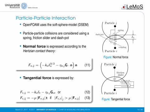
Particle-Particle Interaction• OpenFOAM uses the soft-sphere-model (DSEM)

• Particle-particle collisions are considered using aspring, friction slider and dash-pot

• Normal force is expressed according to theHertzian contact theory :

Fn,ij =(−knδ3/2

n − ηn,jG · n)

n (11)

• Tangential force is expressed by:

Ft,ij = −knδt − ηt,jGct or (12)

Ft,ij = −µ |Fn,ij | t if |Ft,ii |j > µ |Fn,ij | (13)

Figure: Normal force

Figure: Tangential force


LeMoS

Outline





LeMoS

How to build your own Eulerian-Lagrangian Solver inOpenFOAM

• Problem: no proper solver is available for your requirements? /

• Solution: customize an existing solver for your own purposes! ,

Figure: Particle-laden backward-facing step flow according to Fessler & Eaton (1999)


LeMoS


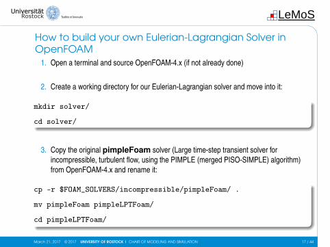
1. Open a terminal and source OpenFOAM-4.x (if not already done)

2. Create a working directory for our Eulerian-Lagrangian solver and move into it:

mkdir solver/

cd solver/

3. Copy the original pimpleFoam solver (Large time-step transient solver forincompressible, turbulent flow, using the PIMPLE (merged PISO-SIMPLE) algorithm)from OpenFOAM-4.x and rename it:

cp -r $FOAM_SOLVERS/incompressible/pimpleFoam/ .

mv pimpleFoam pimpleLPTFoam/

cd pimpleLPTFoam/


LeMoS


4. After moving into the pimpleLPTFoam directory, change the name of the pimpleFoam.Cfile, remove the pimpleDyMFoam and SRFPimpleFoam sub-solver directories:

mv pimpleFoam.C pimpleLPTFoam.C

rm -r pimpleDyMFoam/ SRFPimpleFoam/

mkdir lagrangian

5. Copy the lagrangian library intermediate (includes submodels for particle forces,particle collisions, injection and dispersion models,...) from OpenFOAM-4.x:

cp -r $FOAM_SRC/lagrangian/intermediate/ lagrangian/

6. Open the createFields.H file with a text editor for some customizations:

vi createFields.H


LeMoS


7. Add the following code lines after #include "createMRF.H" to create and readthe fluid density from the transportProperties and calculate the inverse fluid density:

createFields.HInfo« "Reading transportProperties\n" « endl;IOdictionary transportProperties(

IOobject(

"transportProperties",runTime.constant(),mesh,IOobject::MUST_READ_IF_MODIFIED,IOobject::NO_WRITE

));dimensionedScalar rhoInfValue(

transportProperties.lookup("rhoInf"));

dimensionedScalar invrhoInf("invrhoInf",(1.0/rhoInfValue));


LeMoS


8. Create a volScalarField for the fluid density and the dynamic fluid viscosity:

createFields.HvolScalarField rhoInf(

IOobject(

"rho",runTime.timeName(),mesh,IOobject::NO_READ,IOobject::AUTO_WRITE

),mesh,rhoInfValue

);

createFields.HvolScalarField mu(

IOobject(

"mu",runTime.timeName(),mesh,IOobject::NO_READ,IOobject::AUTO_WRITE

),laminarTransport.nu()*rhoInfValue

);


LeMoS


9. Initialize the basicKinematicCollidingCloud (includes particle-particle interactions):

createFields.Hconst word kinematicCloudName(

args.optionLookupOrDefault<word>("cloudName", "kinematicCloud"));Info« "Constructing kinematicCloud " « kinematicCloudName « endl;basicKinematicCollidingCloud kinematicCloud(

kinematicCloudName,rhoInf,U,mu,g

);

10. Open the pimpleLPTFoam.C file for some customizations:

vi pimpleLPTFoam.C


LeMoS

How to build your own Eulerian-Lagrangian Solver inOpenFOAM11. Add the basicKinematicCollidingCloud.H and readGravitationalAcceleration.H to the

existing header files:

pimpleLPTFoam.C...#include "turbulentTransportModel.H"#include "pimpleControl.H"#include "fvOptions.H"#include "basicKinematicCollidingCloud.H"

// * * * * * * * * * * * * * * * * * * * * * * * * * * * * * * * * * * * * * //

int main(int argc, char *argv[]){

#include "setRootCase.H"#include "createTime.H"#include "createMesh.H"#include "readGravitationalAcceleration.H"#include "createControl.H"#include "createTimeControls.H"#include "createFields.H"

...


LeMoS

How to build your own Eulerian-Lagrangian Solver inOpenFOAM12. Add the kinematicCloud.evolve() function after the PIMPLE corrector loop:

pimpleLPTFoam.C// –- Pressure-velocity PIMPLE corrector loopwhile (pimple.loop()){

#include "UEqn.H"

// –- Pressure corrector loop

while (pimple.correct()){

#include "pEqn.H"}if (pimple.turbCorr()){

laminarTransport.correct();turbulence->correct();

}}

Info« "\nEvolving " « kinematicCloud.name() « endl;kinematicCloud.evolve();

runTime.write();


LeMoS

How to build your own Eulerian-Lagrangian Solver inOpenFOAM13. Open the UEqn.H file for some customizations:

vi UEqn.H

14. Expand the momentum equation for two-way coupling:

UEqn.Htmp<fvVectorMatrix> tUEqn(

fvm::ddt(U) + fvm::div(phi, U)+ MRF.DDt(U)+ turbulence->divDevReff(U)==fvOptions(U)+ invrhoInf*kinematicCloud.SU(U)

);fvVectorMatrix& UEqn = tUEqn.ref();

UEqn.relax();


LeMoS

How to build your own Eulerian-Lagrangian Solver inOpenFOAM15. The implementation is (almost) done, but we need some customizations within the

Make directory of the intermediate library in order to compile everything correctly:

vi intermediate/Make/options

16. We want our own customized intermediate library (maybe to implement a own particleforce model or similar), so replace the last code line of the files file by:

filesLIB = $(FOAM_USER_LIBBIN)/libPimpleLPTLagrangianIntermediate

17. Tell the solver where he can find our intermediate library (and some additional too):

vi Make/options


LeMoS

How to build your own Eulerian-Lagrangian Solver inOpenFOAMoptionsEXE_INC =

-Ilagrangian/intermediate/lnInclude \-I$(LIB_SRC)/TurbulenceModels/turbulenceModels/lnInclude \-I$(LIB_SRC)/TurbulenceModels/incompressible/lnInclude \-I$(LIB_SRC)/transportModels \-I$(LIB_SRC)/transportModels/incompressible/singlePhaseTransportModel \-I$(LIB_SRC)/finiteVolume/lnInclude \-I$(LIB_SRC)/meshTools/lnInclude \-I$(LIB_SRC)/sampling/lnInclude \-I$(LIB_SRC)/lagrangian/basic/lnInclude \-I$(LIB_SRC)/regionModels/surfaceFilmModels/lnInclude \-I$(LIB_SRC)/regionModels/regionModel/lnInclude

EXE_LIBS = \-L$(FOAM_USER_LIBBIN) \-lPimpleLPTLagrangianIntermediate \-llagrangian\-lturbulenceModels \-lincompressibleTurbulenceModels \-lincompressibleTransportModels \-lfiniteVolume \

...


LeMoS


18. Tell the compiler the name of our new Eulerian-Lagrangian solver:

vi Make/files

filespimpleLPTFoam.C

EXE = $(FOAM_USER_APPBIN)/pimpleLPTFoam

19. Finally, we can compile the intermediate library and the solver:

wmake all

You received no error messages from the compiler?Congratulations, your new Eulerian-Lagrangian solver is ready...

but how to use it? ,


LeMoS

How to use your own Eulerian-Lagrangian Solver inOpenFOAMParticle-laden backward-facing step flow (Fessler & Eaton, 1999)

• Geometry:

• Step height: H = 26.7mm

• Channel height/width: h = 40mm, B = 457mm

• Length inlet and expansion channel: LU = 5h, LD = 35h

• Flow and particle characteristics:

• Centerline velocity and Reynolds number: U0 = 10.5m/s, Re0 = U0H/ν = 18.600

• Particle type: copper→Dp = 70µm, ρp = 8800 kg/m3

• Stokes number: St = τpτf

= ρpD2pU0/(90µH) = 6.9


LeMoS

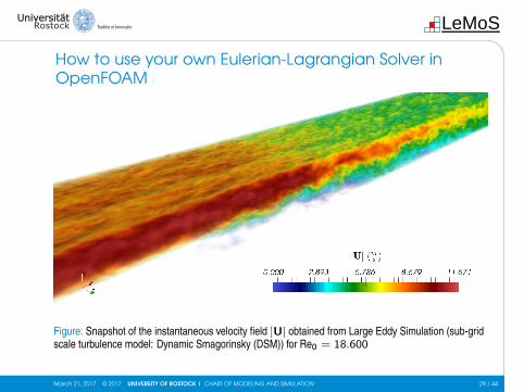
How to use your own Eulerian-Lagrangian Solver inOpenFOAM

Figure: Snapshot of the instantaneous velocity field |U| obtained from Large Eddy Simulation (sub-gridscale turbulence model: Dynamic Smagorinsky (DSM)) for Re0 = 18.600


LeMoS


• Basic folder structure of any OpenFOAM case:

0: includes the initial boundary conditions

constant: includes the mesh (polyMesh folder), physical properties of the fluid(transportProperties), particle properties and settings (kinematicCloudProperties),...

system: includes the simulation settings (controlDict), settings for numerical schemes(fvSchemes) and solver for the algebraic equations systems (fvSolution), decompositionmethods (decomposeParDict), ...

• Download the current tutorial case setup using the git clone command:

Git repository on Bitbucket$ git clone https://[email protected]/slint/gofun2017_particletut.git


LeMoS


1. We start with the mesh generation→ move into the tutorial directory and build the 2Dmesh using OpenFOAM’s blockMesh utility and check the mesh quality:

cd gofun2017_particletutorial/tutorial/BFS/

blockMesh

checkMesh

Figure: Two-dimensional block-structured mesh for the particle-laden backward-facing step flow


LeMoS


2. Let’s see how to define initial boundary conditions (at the example of the velocity field):

Udimensions [0 1 -1 0 0 0 0];

internalField uniform (0 0 0);

boundaryField{

inlet{

type fixedValue;value uniform (9.39 0 0);

}outlet{

type zeroGradient;}walls{

type noSlip;}sides{

type empty;}

}

• OpenFOAM needs the dimension of theflow field in SI-units (see OpenFOAMuser guide)

• You can set an initial flow field if present

• Each patch needs an initial boundarycondition

• Boundary conditions in OpenFOAM:

• Dirichlet (fixedValue)

• Neumann (fixedGradient/zeroGradient)

• Special types: cyclic, symmetry, empty(for 2D caes), ...


LeMoS


3. Let’s see how to set up the particle cloud:

kinematicCloudPropertiessolution{

active true;coupled true;transient yes;cellValueSourceCorrection off;maxCo 0.3;interpolationSchemes{

rho cell;U cell;mu cell;

}integrationSchemes{

U Euler;}

sourceTerms{

schemes{

U semiImplicit 1;}

}

• Activate/de-activate the particle cloud

• Enable/disable phase coupling

• Transient/steady-state solution (max.Courant number)

• Enable/disable correction of momentumtransferred to the Eulerian phase

• Choose interpolation/integrationschemes for the LPT and treatment ofsource terms


LeMoS


kinematicCloudPropertiesconstantProperties{

rho0 8800;youngsModulus 1.3e5;poissonsRatio 0.35;

}

subModels{

particleForces{

sphereDrag;

gravity;

pressureGradient{

U U;}

}

• Define the physical particle properties:

• Density

• Young’s module (elastic modulus)

• Poisson’s ratio

• Define the relevant particle forces:

• Drag force

• Gravition/Buoyancy force

• Pressure drag force


LeMoS


kinematicCloudPropertiesinjectionModels{

model1{

type patchInjection;patchName inlet;duration 1;parcelsPerSecond 33261;massTotal 0;parcelBasisType fixed;flowRateProfile constant 1;nParticle 1;SOI 0.4;U0 (9.39 0 0);sizeDistribution{

type fixedValue;fixedValueDistribution{

value 0.00007;}

}}

}

• Setup of the particle injection:

• Injection model + injection patch name

• Total duration of particle injection

• Injected parcels/particles per second

• Number of particles per parcel

• Start-of-injection time (SOI)

• Initial parcel/particle velocity (U0)

• Size distribution model (normal sizedistribution, ...)


LeMoS


kinematicCloudPropertiesdispersionModel none;

patchInteractionModelstandardWallInteraction;

standardWallInteractionCoeffs{

type rebound;e 0.97;mu 0.09;

}

surfaceFilmModel none;

stochasticCollisionModel none;

collisionModel pairCollision;

• Specify the sub-models for the particlesimulation:

• Turbulent dispersion models (DiscreteRandom Walk model and GradientDispersion model)

• Patch interaction model + coefficients(rebound, stick or escape)

• Surface film model for dripping and filminteraction (absorb, bounce andsplash)

• Stochastic collision/pair collision model(spring, slider and dash-pot)

• Further sub-models: heat transfer (onlyRanz-Marshall correlation), phasechange,...


LeMoS


kinematicCloudPropertiespairCollisionCoeffs{

maxInteractionDistance 0.00007;writeReferredParticleCloud no;pairModel pairSpringSliderDashpot;pairSpringSliderDashpotCoeffs{

useEquivalentSize no;alpha 0.12;b 1.5;mu 0.52;cohesionEnergyDensity 0;collisionResolutionSteps 12;

};wallModel wallSpringSliderDashpot;wallSpringSliderDashpotCoeffs{

useEquivalentSize no;collisionResolutionSteps 12;youngsModulus 1e10;poissonsRatio 0.23;alpha 0.12;b 1.5;mu 0.43;cohesionEnergyDensity 0;

};

}

• Adjust the particle-particle andparticle-wall interaction modelcoefficients:

• α: coefficient related to the coefficientof restitution e (see diagram)

• b: Spring power→ b = 1 (linear) orb = 3/2 (Hertzian theory)

• µ: friction coefficient

0.01 0.05 0.1 0.5 1 50

0.2

0.4

0.6

0.8

1

α [-]

e[-]

Figure: Relationship between α and the coefficientof restitution e (Tsuji et al., 1992)


LeMoS


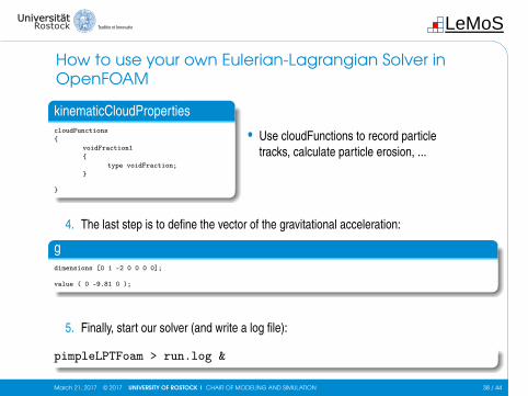
kinematicCloudPropertiescloudFunctions{

voidFraction1{

type voidFraction;}

}

• Use cloudFunctions to record particletracks, calculate particle erosion, ...

4. The last step is to define the vector of the gravitational acceleration:

gdimensions [0 1 -2 0 0 0 0];

value ( 0 -9.81 0 );

5. Finally, start our solver (and write a log file):

pimpleLPTFoam > run.log &


LeMoS


6. Use OpenFOAM’s foamMonitor utility to check the convergence:

foamMonitor -l postProcessing/residuals/0/residuals.dat


LeMoS

Post-Processing with OpenFOAM/Paraview• OpenFOAM provides many utilities (e.g. sampling of data) and functionObjects (e.g.

calculation of forces and turbulence fields) for the analysis of simulation results

• The standard program for the graphical post-processing of OpenFOAM cases isParaview (see OpenFOAM user guide)

1. Start post-processing with Paraview by typing:

paraFoam

2. Load the last time step and check the velocity and pressure field:


LeMoS

Post-Processing with OpenFOAM/Paraview

3. Let’s check how much volume of each grid cell is occupied by particles (void fractionα = Vp/Vc ):


LeMoS

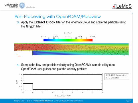
Post-Processing with OpenFOAM/Paraview3. Apply the Extract Block filter on the kinematicCloud and scale the particles using

the Glyph filter:

4. Sample the flow and particle velocity using OpenFOAM’s sample utility (seeOpenFOAM user guide) and plot the velocity profiles:

−2 0 2 4 6 8 10 12 14

0

0.5

1

1.5

2

2.5

2 · 〈Up,x 〉/U0 + x/H

y/H

EFD: LDA (Fessler et al.)CFD Simulation


LeMoS

Further Information and References

OpenFOAM User/Programmers Guide (www.openfoam.org)

Crow, T. C., Schwarzkopf, J. D., Sommerfeld, M. and Tsuji, Y., 2011, Multiphase flowswith droplets and particles, 2nd ed., CRC Press, Taylor & Francis.

Sommerfeld, M., 2010, Particle Motion in Fluids, VDI Heat Atlas, Springer.

Elghobashi, S., 1994, On predicting particle-laden turbulent flows, Applied ScientificResearch, Vol. 52, pp. 309-329.

Fessler, J. R. and Eaton, J. K., 1999, Turbulence modification by particles in abackward-facing step flow, J. Fluid Mech., Vol. 394, pp. 97-117.

Tsuji, Y., Tanaka, T. and Ishida, T., 1992, Lagrangian numerical simulation of plug flowof collisionless particles in a horizontal pipe, Powder Tech., Vol. 71, 239.


LeMoS

Thank you for your attention!

Any questions?

Robert Kasper, M.Sc.

University of Rostock

Faculty of Mechanical Engineering and Marine Technology

Chair of Modeling and Simulation

Albert-Einstein-Str. 2

18059 Rostock

Email: [email protected]


german openfoam user meeting 2017 (gofun 2017 ... · pdf filegerman openfoam user meeting 2017...

Documents