· long-time asymptotics for the camassa–holm equation anne boutet de monvel, aleksey kostenko,...

LONG-TIME ASYMPTOTICS FOR THE CAMASSA–HOLM

EQUATION

ANNE BOUTET DE MONVEL, ALEKSEY KOSTENKO, DMITRY SHEPELSKY,AND GERALD TESCHL

Abstract. We apply the method of nonlinear steepest descent to compute the long-time asymptotics of the Camassa–Holm equation for decaying initial data, completingprevious results by A. Boutet de Monvel and D. Shepelsky.

1. Introduction

In this paper we want to study the long-time asymptotics of the Camassa–Holm(CH) equation, also known as the dispersive shallow water equation,

ut + 2κux − utxx + 3uux = 2uxuxx + uuxxx, t > 0, x ∈ R, (1.1)

where u ≡ u(x, t) is the fluid velocity in the x direction, κ > 0 is a constant relatedto the critical shallow water wave speed, and subscripts denote partial derivatives. Itwas first introduced by R. Camassa and D. Holm in [7] and R. Camassa et al. [8] as amodel for shallow water waves, but already appeared earlier in a list by B. Fuchssteinerand A. Fokas [19]. More on the hydrodynamical relevance of this model can be foundin the recent articles by R. Johnson [22] and A. Constantin and D. Lannes [12]. With

w := u − uxx + κ, (1.2)

called the “momentum”, equation (1.1) can be expressed as the condition of compati-bility between

1

w

(−f ′′ +

1

4f

)= λf, (1.3)

and

∂tf = −(

1

2λ+ u

)f ′ +

1

2u′f, (1.4)

that is,

∂t∂xxf = ∂xx∂tf

is the same as saying that (1.1) holds. Equation (1.3) is the spectral problem associatedto (1.1). In particular, the CH equation is completely integrable and can be solved

Date: September 25, 2009.2000 Mathematics Subject Classification. Primary 37K40, 35Q35; Secondary 37K45, 35Q15.Key words and phrases. Camassa–Holm equation, Riemann–Hilbert problem, solitons.Research supported (G.T.) by the Austrian Science Fund (FWF) under Grant No. Y330.SIAM J. Math. Anal. 41:4, 1559–1588 (2009).

1

2 A. BOUTET DE MONVEL, A. KOSTENKO, D. SHEPELSKY, AND G. TESCHL

via the inverse scattering method. Correspondingly, we consider real-valued classicalsolutions u(x, t) of the CH equation (1.1), which decay rapidly, that is,

max0<t≤T

∫

R

(1 + |x|)l+1(|w(x, t) − κ| + |wx(x, t)| + |wxx(x, t)|

)dx < ∞ (1.5)

for all T > 0 and some integer l ≥ 1. Moreover, we will assume

w(x, 0) > 0 (1.6)

throughout this paper. Then u exists for all times t > 0 with w(x, t) > 0 (for exis-tence of solutions we refer to A. Constantin and J. Escher [10] and the discussion inA. Constantin and J. Lenells [13], see also [9]).

The aim of this paper is to establish the long-time asymptotics of such solutionsusing the nonlinear steepest descent method from P. Deift and X. Zhou [16] which wasinspired by earlier work of S. Manakov [27] and A. Its [21]. More on this method andits history can be found in the survey by P. Deift, A. Its, and X. Zhou [17].

The starting point for this method is the representation of a solution of the nonlinearequation under consideration in terms of a solution of an associated Riemann-Hilbertproblem.

Recently, A. Boutet de Monvel and D. Shepelsky have used the inverse scatteringapproach to the CH equation, based on the construction and analysis of an associatedmatrix Riemann-Hilbert problem [3, 4]. The analysis, via the nonlinear steepest descentmethod, of a vector oscillatory RH problem derived from the original matrix-valuedproblem, allowed [5] distinguishing four main regions in the (x, t)-half-plane, where theleading asymptotic terms were qualitatively different: a solitonic sector, two sectors of(slowly decaying) modulated oscillations, and a sector of rapid decay.

Here we want to simplify the original approach, deriving the vector Riemann-Hilbertproblem directly from scattering theory for the underlying Sturm–Liouville operator.We notice that the matrix and vector RH problems, being closely related, have specificfeatures concerning, particularly, the uniqueness issue. For the matrix problem, werefer to [5], whereas the uniqueness for the vector problem is addressed in detail in thepresent paper, see Section 3 below.

At the same time we want to provide complete proofs including the effects of solitonsin the sectors of decaying oscillations (formulas given in [5] for the oscillatory regionsare true in the solitonless case only) and the error estimates in terms of decay of theinitial condition. Moreover, we will make use of some simplifications to the nonlinearsteepest descent method recently given in H. Kruger and G. Teschl [24] respectivelyK. Grunert and G. Teschl [20].

The asymptotics in the transition regions, near the lines x/κt = 2 and x/κt = −1/4,involves Painleve transcendents. A detailed analysis is presented in [1].

2. Main result

In order to state our main result we first need to recall a few things.

LONG-TIME ASYMPTOTICS FOR THE CH EQUATION 3

Scattering data. Associated with w(x, t) is a self-adjoint Sturm–Liouville operator

H(t) =1

w(x, t)

(− d2

dx2+

1

4

),

D(H(t)

)= H2(R) ⊂ L2(R, w dx).

(2.1)

Here L2(R, w dx) denotes the Hilbert space of square integrable (complex-valued) func-tions over R and H2(R) the corresponding Sobolev space.

By our assumption (1.5) the spectrum of H(t) (independent of t) consists of anabsolutely continuous part [ 1

4κ,∞) plus a finite set of eigenvalues λj ∈ (0, 1

4κ), 1 ≤

j ≤ N , possibly empty (“solitonless case”), see [9, Theorem 2.1]. For j = 1, . . . , N wedenote

λj =1

κ

(1

4− κ2

j

),

0 < κ1 < κ2 < · · · < κN <1

2.

Moreover, associated with the continuous spectrum is a (right) reflection coefficientR+(k, t), and associated with every eigenvalue λj is a (right) norming constant γ+,j(t)(see the next section for details).

One-soliton solution. Given κ ∈ (0, 12) and γ > 0 we have the corresponding one-

soliton solution u(κ,γ)sol

≡ usol(x, t) given by

usol(x − κct) =32κκ2

(1 − 4κ2)2α(y(x − κct))

(1 + α(y(x − κct)))2 + 16κ2

1−4κ2 α(y(x − κct)), (2.2)

with

α(y) =γ2

2κe−2κy, (2.3a)

c =1

2(14 − κ2)

∈ (2,∞), (2.3b)

where y(x) is given implicitly by

x = y + log1 + α(y)1+2κ

1−2κ

1 + α(y)1−2κ1+2κ

. (2.4)

The momentum w(κ,γ)sol

≡ wsol(x, t) of this solution is given by

wsol(x − κct) = κ

(1 +

16κ2

1 − 4κ2

α(y(x − κct))

(1 + α(y(x − κct)))2

)2

. (2.5)

Note that the one-soliton solution has the form of a single peak which is symmetricwith respect to its center

x0 =1

2κlog

γ2

2κ+ log

1 + 2κ

1 − 2κ.


The maximum at x0 is given by usol,max = κ8κ2

1−4κ2 and taller waves are narrower and

travel faster (for fixed κ). See Fig. 1, where usol(x−x0) for fixed κ and different valuesof κ is displayed.

-

6

x

usol(x)

.

..............

..............

................

..............

.................

..............

.................

................

....................

....................

........................

...........................

............

...............

.................

....................

....................................................................

...................

................

............

.........

......

............

.........

........

...... .....

.

........

..

..

..

..

.

..

..

..

..

..

..

..

..

..

..

..

..

..

.

..

..

..

..

..

..

..

..

..

..

..

..

..

..

..

..

..

..

..

..

..

..

..

.

..

..

..

..

..

..

..

..

..

..

..

..

..

..

..

..

..

..

..

..

..

..

..

..

..

..

..

..

..

..

..

..

..

..

..

..

..

..

..

..

..

..

..

..

..

..

..

..

..

..

..

..

.

..

..

..

..

..

..

..

.

..

..

..

..

..

..

..

..

..

..

..

..

..

..

..

..

..

..

..

.

..

..

..

..

..

..

..

..

..

..

..

..

..

..

..

..

..

..

..

..

..

..

..

..

..

..

..

..

..

..

..

..

..

..

..

..

..

..

..

..

.................

..............

.................

..............

................

..............

..............

................................................

...........

...........

.....

.....

.....

...........

.....

.....

.....

..........

.........

.....

.

....

.

....

.

.

....

.

....

.

....

.

....

.

....

.

....

.

.

.....

.

....

.

....

.....

.

..

.

...

.

.....

.....

.

....

.....

.....

...................................

.....

....

..........

.

..

..

.

.

..

..

.

.

.

..

....

.....

.

..

..

.

..

..

.

.

..

..

.

.

.

..

..

.

..

..

.

..

..

.

..

..

.

..

..

.

..

..

.

.

..

..

.

..

..

.....

.........

..........

.....

.....

.....

...........

.....

.....

.....

...........

...........

.................................................

................................................................................................................ ..... ........... ..... ..... ..... ..... ..... ..... ........... ..... .....

............................................................................................

Figure 1. One-solitons for fixed κ = 1 and κ = .15, .25, .3

Note also that if κ = κ(κ) is changing in such a way that the soliton velocity

v = cκ =2κ

1 − 4κ2

is fixed, then, as κ → 0, the form of the soliton approaches that of a peakon, ve−|x|,which is a nonsmooth, weak solution of the Camassa–Holm equation with κ = 0(see [4]). See Fig. 2, where usol(x − x0) for fixed velocity v and different values of(κ, κ) is displayed. Note that usol,max = v − 2κ.

-

6

x

usol(x)

. ................. ..................................

..................

..................

..................

..........

.........

...........

.........

...........

.........

............

..........

...............

..............

.....................

....................

..............................

.

.

.

.

.

.

.

.

.

.

.

.

.

.

.

.

.

.

.

.

.

.

.

.

.

.

.

.

.

.

...

.

.

.

.

.

.

.

.

.

.

.

.

.

.

.

.............

..

..

...

..

...

...

.

.

.

..

.

.

.

.

.

..

.

.

.

.

.

..

.

.

.

.

.

.

.

.

.

.

.

.

.

.

.

.

.

.

.

.

.

.

.

.

.

.

.

.

.

.

.

.

.

.

.

.

.

.

.

.

.

.

.

.

.

.

.

.

.

.

.

.

.

.

.

.

.

.

.

.

.

.

.

.

.

.

.

.

.

.

.

.

.

.

.

.

.

.

.

.

.

.

..

...

..

...

..

.

.

.

.

.

.

.

.

.

.

......

....

..

..

..

.

.

.

.

.

.

.

.

.

..

..

..

.

..

..

.

.

.

.

.

.

.

.

.

.

.

.

.

.

.

.

.

.

.

.

.

.

.

.

.

.

.

.

.

.

.

.

.

.

.

.

.

.

.

.

.

.

.

.

.

.

.

.

.

.

.

.

.

.

.

.

.

.

.

.

.

.

.

.

.

.

.

.

.

.

.

.

.

.

.

.

.

.

.

.

.

.

.

..

.

.

.

.

..

.

.

.

.

..

.

.

.

.

.

..

.

..

..

.

..

.

..

.

..

..

..

..

..

..

..

.

..

..

..

..

..

.

.

.

.

.

.

..

.

.

.

.

.

.

.

.

.

.

.

.

.

.

.

.

.

.

.

.

.

.

.

.

.

.

.

.

.

.

.

..

..

..

..

..

..

..

..

..

..

..

..

..

..

..

..

..

..

..

..

..

..

..

..

..

..

..

..

..

..

..

..

..

..

..

.

..

..

..

..

..

..

..

..

..

..

..

..

..

..

.

..........

............

.........

...........

.........

...........

.........

..........

..................

..................

.................. ................. ................. ............................

............................................................................

.....

...........

..........

.....

.

....

.

....

.

.

....

.

....

.

.

....

.

....

.

....

.

.

....

.

....

.

....

.

.

...

.

...

.

....

.

....

.

....

.

.

....

.

....

.

....

.

....

.

....

.

....

.

....

.

....

.

....

.

....

.

....

.

......

.

......

.

.

.....

.

....

.

....

.

.

...

.

..

.

...

.................

.

..

.

...

.

..

.

.

..

..

.

..

..

.

.

..

..

.

.

..

..

..

.

..

..

..

.

.

..

..

.

..

..

.

..

..

.

..

..

.

..

..

.

..

..

.

..

..

.

..

..

.

..

..

.

.

..

..

.

..

..

.

..

..

.

..

..

.

..

..

.

.

..

.

.

..

.

.

..

..

.

..

..

.

..

..

.

..

..

.

..

..

.

..

..

.

..

..

.

..

..

.

..

..

.

..

..

....

....

.....

.....

.....

............

..............................................................................

........................................................

.....

.....

.....

.....

.....

.....

.....

.....

.......................................... ..... ..... ......

.........

................

.....

.....

.....

.....

.....

.....

.....

.....

.................................................... .....

Figure 2. Fixed velocity v = 2.5 and (κ, κ) = (1, .22), (.5, .39), (.1, .48)

Now we are ready to state our main result.

Theorem 2.1 (solution asymptotics). Suppose u(x, t) is a classical solution of the CHequation (1.1) satisfying (1.5) for some integer l ≥ 1. Let

R(k) = R+(k, 0) and κj , γj = γ+,j(0), j = 1, . . . , N,

be the (right) scattering data associated with H(0) and the initial condition w(x, 0).There are four sectors in the (x, t) half-plane in which the long-time asymptotics of

a solution of the CH equation satisfying (1.5) are given by the following formulas:


(i) The “soliton” region c := xκt > 2 + C for any small C > 0. Let

cj =1

2(14 − κ2

j ), j = 1, . . . , N,

and let ε > 0 sufficiently small such that the intervals [cj − ε, cj + ε] are disjointand lie inside (2,∞).(i1) If | x

κt − cj | < ε for some j, one has

u(x, t) = uj(x − ξj − κcjt) + O(t−l), (2.6)

where uj = u(κj ,γj)sol

is the one-soliton solution formed from κj and

γj = γj

N∏

i=j+1

κi − κj

κi + κj, (2.7)

and having a phase shift

ξj = 2N∑

i=j+1

log1 + 2κi

1 − 2κi. (2.8)

For j = N the product is 1 in (2.7) and the sum is 0 in (2.8).(i2) If

∣∣ xκt − cj

∣∣ ≥ ε for all j, one has

u(x, t) = O(t−l). (2.9)

(ii) The “first oscillatory” region 0 ≤ c := xκt < 2 − C for any C > 0. Here

u(x, t) = −√

2κk0(c)ν0(c)

(14 + k0(c)2)(

34 − k0(c)2)t

sin

(2κk0(c)

3

(14 + k0(c)2)2

t − ν0(c) log(t) + δ0(c)

)

+ O(t−α) (2.10)

for any 12 < α < 1 provided l ≥ 5, where

k0(c) =1

2

√

−1 + c −√

1 + 4c

c, (2.11)

ν0(c) = − 1

2πlog(1 − |R(k0(c))|2), (2.12)

δ0(c) =π

4− arg(R(k0(c))) + arg(Γ(iν0(c)))

− ν0(c) log

(8κk0(c)

2(3/4 − k0(c)2)

(1/4 + k0(c)2)3

)

+ 4N∑

j=1

arctan( κj

k0(c)

)+

1

π

∫

Σ(c)log(|ζ − k0(c)|) d log(1 − |R(ζ)|2)

+ 4κk0(c)

N∑

j=1

log

(1 + 2κj

1 − 2κj

)+

4κk0(c)

π

∫

Σ(c)

log(|T (ζ)|2)1 + 4ζ2

dζ, (2.13)


with Σ(c) = (−k0(c), k0(c)) and Γ the Gamma function.

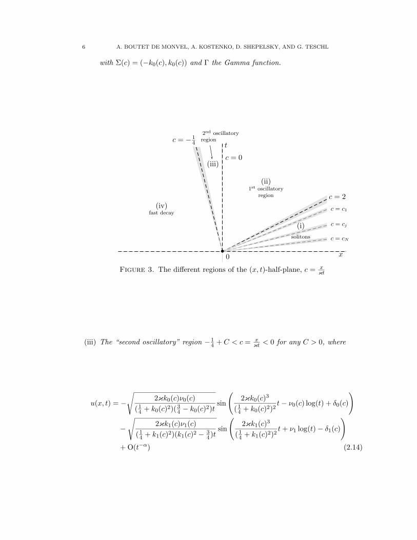
•0

c = cN

c = cj

c = c1

c = 2

c = 0

c = −14

(i)

solitons

(ii)1st oscillatory

region

(iii)

2nd oscillatoryregion

(iv)fast decay

x

t

Figure 3. The different regions of the (x, t)-half-plane, c = xκt

(iii) The “second oscillatory” region −14 + C < c = x

κt < 0 for any C > 0, where

u(x, t) = −√

2κk0(c)ν0(c)

(14 + k0(c)2)(

34 − k0(c)2)t

sin

(2κk0(c)

3

(14 + k0(c)2)2

t − ν0(c) log(t) + δ0(c)

)

−√

2κk1(c)ν1(c)

(14 + k1(c)2)(k1(c)2 − 3

4)tsin

(2κk1(c)

3

(14 + k1(c)2)2

t + ν1 log(t) − δ1(c)

)

+ O(t−α) (2.14)


for any 12 < α < 1 provided l ≥ 5. Here, for ℓ = 0, 1,

kℓ(c) =1

2

√

−1 + c − (−1)ℓ√

1 + 4c

c, (2.15)

νℓ(c) = − 1

2πlog(1 − |R(kℓ(c))|2), (2.16)

δℓ(c) =π

4− (−1)ℓ arg(R(kℓ(c))) + arg(Γ(iνℓ(c)))

− νℓ(c) log(−1)ℓ8κkℓ(c)

2(3/4 − kℓ(c)2)

(1/4 + kℓ(c)2)3+ (−1)ℓ4

N∑

j=1

arctanκj

kℓ(c)

+(−1)ℓ

π

∫

Σ(c)log(|ζ − kℓ(c)|)d log(1 − |R(ζ)|2)

+ (−1)ℓ2νℓ′(c) logk1(c) − k0(c)

k1(c) + k0(c)

+ 4κkℓ(c)N∑

j=1

log1 + 2κj

1 − 2κj+

4κkℓ(c)

π

∫

Σ(c)

log(|T (ζ)|2)1 + 4ζ2

dζ, (2.17)

with Σ(c) = (−∞,−k1(c)) ∪ (−k0(c), k0(c)) ∪ (k1(c),∞), 0′ = 1, and 1′ = 0.(iv) The “fast decay” region c = x

κt < −14 − C for any C > 0, where

u(x, t) = O(t−l). (2.18)

We can also give the asymptotics of the momentum w(x, t).

Theorem 2.2 (momentum asymptotics). Under the same hypotheses and with thesame notations the momentum of the solution behaves as follows:

(i) In the soliton region c = xκt > 2 + C.

(i1) If | xκt − cj | < ε for some j, one has

w(x, t) = wj(x − ξj − κcjt) + O(t−l) (2.19)

where wj is the momentum of the one-soliton solution formed from the sameparameters {κj , γj} and with the same phase shift ξj as above.

(i2) If | xκt − cj | ≥ ε for all j, one has

w(x, t) = κ + O(t−l). (2.20)

(ii) In the first oscillatory region 0 ≤ c = xκt < 2 − C for any C > 0, one has

w(x, t) = κ − 4

√2κk0(c)(

14 + k0(c)2)ν0(c)

(34 − k0(c)2)t

sin

(2κk0(c)

3

(14 + k0(c)2)2

t − ν0(c) log(t) + δ0(c)

)

+ O(t−α), (2.21)

for any 12 < α < 1 provided l ≥ 5.


(iii) In the second oscillatory region −14 + C < c = x

κt < 0 for any C > 0, one has

w(x, t) = κ − 4

√2κk0(c)(

14 + k0(c)2)ν0(c)

(34 − k0(c)2)t

sin

(2κk0(c)

3

(14 + k0(c)2)2

t − ν0(c) log(t) + δ0(c)

)

− 4

√2κk1(c)(

14 + k1(c)2)ν1(c)

(k1(c)2 − 34)t

sin

(2κk1(c)

3

(14 + k1(c)2)2

t + ν1(c) log(t) − δ1(c)

)

+ O(t−α), (2.22)

for any 12 < α < 1 provided l ≥ 5.

(iv) In the fast decay region xκt < −1

4 − C for any C > 0, we have

w(x, t) = κ + O(t−l). (2.23)

In particular we recover the fact that a pure soliton solution (i.e., R(k) ≡ 0) asymp-totically splits into single solitons with associated phase shifts. This was shown onlyrecently by R.S. Johnson [23] (for two solitons) and in the general case by Y. Matsuno[29]. For further results on solitons of the CH equation and their stability we refer toA. Constantin and W. Strauss [14], L.-C. Li [26], and K. El Dika and L. Molinet [18].

Notice that the oscillatory regions (ii) and (iii) match at x = 0. Indeed, as x → 0with x < 0, k1 → ∞ in (2.15) and thus the amplitude of the second term in (2.14)vanishes, while the parameters of the first term in (2.14) match those in (2.10). Asfor the transition between the other regions, we have already noticed in Section 1 thatthere exist transition zones, where the asymptotics are described in terms of Painlevetranscendents. More precisely (details are given in [1]), these zones are:

(tr1) |x/κt − 2| t2/3 < Const,

(tr2) |x/κt + 1/4| t2/3 < Const.

It should also be emphasized that unlike the (modified) Korteweg–de Vries (KdV)equation (originally considered in [16]), the asymptotic form is given implicitly, however,to leading order this fact only manifests itself in additional phase shift. More precisely,the term ξj in the soliton region (as already pointed out in [29]) and the last two termsin δj(c), have no analog in the (modified) KdV equation (cf. [16], respectively [20]).For results on CH on the half-line we refer to A. Boutet de Monvel and D. Shepelsky[2, 6].

Finally, note that if u(x, t) solves the CH equation, then so does u(−x,−t). Thereforeit suffices to investigate the case t → +∞.

3. The Inverse scattering transform and the Riemann–Hilbert problem

In this section we derive a vector Riemann–Hilbert problem directly from the scat-tering theory for the differential operator (1.3). We begin by recalling some requiredresults from scattering theory, respectively the inverse scattering transform for the CHequation from [9, 11] (see also [28]).


Recall also that by virtue of the unitary Liouville transform

f(x) 7→ f(y) = w(x)1/4f(x),

y = x −∫ +∞

x

(√w(r)

κ− 1

)dr,

(3.1)

the Sturm–Liouville operator H(t) introduced in (2.1) can be mapped to a self-adjointSchrodinger operator

H(t) =1

κ

(− d2

dy2+ q( · , t) +

1

4

),

D(H(t)

)= H2(R) ⊂ L2(R).

(3.2)

where

q(y, t) =κ

4

wxx(x, t)

w(x, t)2− w(x, t) − κ

4w(x, t)− 5κ

16

wx(x, t)2

w(x, t)3.

From our assumption (1.5) it follows that q(y, t) ∈ L1(R, (1 + |y|)l+1dy).

Lemma 3.1. There exist two Jost solutions ψ±(k, x, t) which solve the differentialequation

H(t)ψ±(k, x, t) =1

κ

(1

4+ k2

)ψ±(k, x, t), Im(k) ≥ 0, (3.3)

andlim

x→±∞e∓ikxψ±(k, x, t) = 1. (3.4)

Both ψ±(k, x, t) are analytic for Im(k) > 0 and continuous for Im(k) ≥ 0. For large kwe have

ψ±(k, x, t) = e±ik(y+ 1∓12

H−1(w)) κ1/4

w(x, t)1/4

(1 ∓

∫ ±∞

yq(r, t)dr

1

2ik+ O

( 1

k2

))(3.5)

as k → ∞, where

H−1(w) =

∫

R

(√w(r)

κ− 1

)dr (3.6)

is a conserved quantity of the CH equation.

Proof. This is immediate from the corresponding results for (3.2) (cf., e.g., [15] or [28])by virtue of our Liouville transform (3.1). Just observe

ψ±(k, x, t) = e−ik 1∓12

H−1(w) κ1/4

w(x, t)1/4ψ±(k, y, t),

where ψ±(k, y, t) are the Jost solutions of (3.2). ¤

Furthermore, one has the scattering relations

T (k)ψ∓(k, x, t) = ψ±(k, x, t) + R±(k, t)ψ±(k, x, t), k ∈ R, (3.7)

where T (k), R±(k, t) are the transmission, resp. reflection coefficients. We have sym-metry relations

R±(−k, t) = R±(k, t) and T (−k) = T (k).


Note also that if T (k), R±(k, t) are the corresponding quantities for H(t), then T (k) =

eikH−1(w)T (k), R+(k, t) = R+(k, t), and R−(k, t) = e2ikH−1(w)R−(k, t) and hence allresults known for (3.2) readily apply in our situation. In particular, they have thefollowing well-known properties:

Lemma 3.2. The transmission coefficient T (k) is meromorphic for Im(k) > 0 with

simple poles at iκ1, . . . , iκN , where as above κj =√

14 − κλj ∈ (0, 1

2), and is continuous

up to the real line. Asymptotically we have

T (k) = eikH−1(w)(1 + O(k−1)). (3.8)

The residues of T (k) are given by

Resiκj T (k) = iµj(t)γ+,j(t)2 = iµjγ

2+,j , (3.9)

where

γ+,j(t)−2 = κ

−1

∫

R

ψ+(iκj , r, t)2w(r, t)dr (3.10)

and ψ+(iκj , x, t) = µj(t)ψ−(iκj , x, t).Moreover,

T (k)R+(k, t) + T (k)R−(k, t) = 0, |T (k)|2 + |R±(k, t)|2 = 1. (3.11)

Note that one reflection coefficient, say R(k, t) = R+(k, t), and one set of normingconstants, say γj(t) := γ+,j(t), suffices.

The time dependence is given by (see [9]):

Lemma 3.3. The time evolutions of the quantities R(k, t) and γj(t) are given by,

R(k, t) = R(k)e−i κk

1/4+k2 t, (3.12)

γj(t) = γje

κκj/2

1/4−κ2j

t(3.13)

where R(k) = R(k, 0) and γj = γj(0).

Vector Riemann–Hilbert problem. We will set up a vector Riemann–Hilbert prob-lem as follows. Let m(k, x, t) =

(m1(k, x, t) m2(k, x, t)

)be defined by

(w(x,t)κ

)1/4(T (k)ψ−(k, x, t)eiky ψ+(k, x, t)e−iky

), Im(k) > 0,

(w(x,t)κ

)1/4(ψ+(−k, x, t)eiky T (−k)ψ−(−k, x, t)e−iky

), Im(k) < 0.

(3.14)

We are interested in the jump condition of m(k, x, t) on the real k-axis (oriented fromnegative to positive). To formulate our jump condition we use the following convention:when representing functions on R, the lower subscript denotes the non-tangential limitfrom different sides. By m+(k) we denote the limit from above and by m−(k) the onefrom below. Using the notation above implicitly assumes that these limits exist in thesense that m(k) extends to a continuous function on the real axis. In general, for anoriented contour Σ, m+(k) (resp. m−(k)) will denote the limit of m(κ) as κ → k fromthe positive (resp. negative) side of Σ. Here the positive (resp. negative) side is the onewhich lies to the left (resp. right) as one traverses the contour in the direction of theorientation.


Theorem 3.4 (vector RH-problem). Let S+(H(0)) = {R(k), (κj , γj), j = 1, . . . , N} bethe right scattering data of the operator H(0) associated with the initial data w(x, 0).Then m(k) ≡ m(k, x, t) defined in (3.14) is a solution of the following vector Riemann–Hilbert problem. Find a function m(k) which satisfies:

(i) The analyticity condition:m(k) is meromorphic away from the real axis with simple poles at ±iκj.

(ii) The jump condition, for k ∈ R:

m+(k) = m−(k)v(k),

v(k) =

(1 − |R(k)|2 −R(k)e−tΦ(k)

R(k)etΦ(k) 1

).

(3.15)

(iii) The pole conditions, for j = 1, . . . , N :

Resiκj m(k) = limk→iκj

m(k)

(0 0

iγ2j etΦ(iκj) 0

). (3.16)

In (ii) and (iii) the phase is given by

Φ(k) = −iκk

14 + k2

+ 2iky

t. (3.17)

(iv) The symmetry condition

m(−k) = m(k)

(0 11 0

). (3.18)

(v) The normalization

limk→∞

m(k) = (1 1). (3.19)

Remarks. (a) Note that det v(k) ≡ 1 and v(−k) = σ1v(k)−1σ1 with σ1 = ( 0 11 0 ).

(b) Note also that (iii) and (iv) imply the pole conditions, for j = 1, . . . , N :

Res−iκj m(k) = limk→−iκj

m(k)

(0 −iγ2

j etΦ(iκj)

0 0

).

Proof. The jump condition (3.15) is a simple calculation using the scattering relations(3.7) plus (3.11). The pole conditions follow since T (k) is meromorphic for Im(k) > 0with simple poles at iκj and residues given by (3.9). The symmetry condition holds byconstruction and the normalization (3.19) is immediate from (3.5) and

T (k) = eikH−1(w)

(1 +

∫ +∞

−∞q(r, t)dr(2ik)−1 + O(k−2)

)(3.20)

which implies

m(k, x, t) =(1 1

)+ Q+(y, t)

1

2ik

(1 −1

)+ O(k−2), (3.21)

where Q+(y, t) =∫ +∞y q(r, t)dr. ¤


Observe that the pole condition at iκj is sufficient since the one at −iκj follows bysymmetry. Hence, the Riemann–Hilbert problem for the Camassa–Holm equation is,for given scattering data S+, to find a sectionally meromorphic vector function m(k)satisfying (3.15)–(3.19). We will show that the solution given in the above theoremis in fact the only one in Corollary 3.9 below. Moreover, it should be pointed outthat except for the phase, this Riemann–Hilbert problem is identical to the one for theKorteweg–de Vries equation (cf. [20, Thm. 2.3]).

Next we note the following useful asymptotics

Lemma 3.5. The function m(k, x, t) defined in (3.14) satisfies

m1(i2 , x, t)

m2(i2 , x, t)

= ex−y, (3.22)

and

m1(k, x, t)m2(k, x, t) =

√w(x, t)

κ

(1 + 2i

κu(x, t)

(k − i

2

)+ O(k − i

2)2). (3.23)

Proof. The Jost solutions admit the representation ψ±(k, x, t) = e±ikxg±(k, x, t), whereg±(k, x, t) are the solutions of the integral equations

g±(k, x, t) = 1 ± k2 + 14

2iκk

∫ ±∞

x(1 − e∓2ik(x−r))g±(k, r, t)(w(r, t) − κ)dr. (3.24)

Since w satisfies (1.5), the solution of (3.24) exists and is unique (see, for example,[28]). Moreover, g± is analytic for Im(k) > 0.

Since k2 + 14 = (k − i

2)(k + i2), we get

g±(k, x, t) = 1 ± i

κ(k − i

2)F±(x, t) + O(k − i2)2, k → i/2, (3.25)

where

F±(x, t) =

∫ ±∞

x(e±(x−r) − 1)(w(r, t) − κ)dr. (3.26)

Moreover, differentiating with respect to x, we see

g′±(k, x, t) = ± i

κ(k − i

2)F ′±(x, t) + O(k − i

2)2, (3.27)

with

F ′±(x, t) = ±

∫ ±∞

xe±(x−r)(w(r, t) − κ)dr. (3.28)

Using

u(x, t) =(1 − ∂2

x

)−1(w(x, t) − κ) =

1

2

∫

R

e−|x−r|(w(r, t) − κ)dr, (3.29)

we thus obtain

ψ+(k, x, t)ψ−(k, x, t) = 1 +i

κ(F+(x, t) − F−(x, t))(k − i

2) + O(k − i2)2

= 1 +i

κ(2u(x, t) − H0(u))(k − i

2) + O(k − i2)2, (3.30)


where

H0(u) =

∫

R

(w(x, t) − κ)dx =

∫

R

u(x, t)dx (3.31)

is a conserved quantity of the CH equation.Furthermore, straightforward calculations show that

T (k)−1 =W(ψ−, ψ+)

2ik

= 1 +i

κ

(F+(x, t) − F−(x, t) − F ′

+(x, t) − F ′−(x, t)

)(k − i

2) + O(k − i2)2

= 1 − i

κH0(u)(k − i

2) + O(k − i2)2, (3.32)

where W(f, g) = fg′ − f ′g is the usual Wronskian. Therefore,

T (k) = 1 +i

κH0(u)

(k − i

2

)+ O

(k − i

2

)2. (3.33)

Substituting (3.25) and (3.33) into (3.14), we arrive at (3.22). Substituting (3.30) and(3.33) into (3.14), we obtain (3.23). ¤

Regular Riemann–Hilbert problem. For our further analysis it will be convenientto rewrite the pole condition as a jump condition and hence turn our meromorphicRiemann–Hilbert problem into a holomorphic Riemann–Hilbert problem.

Choose ε so small that the discs |k − iκj | < ε lie inside the upper half plane and donot intersect. Then redefine m(k) in a neighborhood of iκj , resp. −iκj according to

m(k) =

m(k)

1 0

− iγ2j etΦ(iκj)

k−iκj1

, |k − iκj | < ε,

m(k)

1

iγ2j etΦ(iκj)

k+iκj

0 1

, |k + iκj | < ε,

m(k), else.

(3.34)

Note that we redefined m(k) such that it respects our symmetry (3.18).Then a straightforward calculation using Resiκ m(k) = limk→iκ(k − iκ)m(k) shows:

Lemma 3.6 (regular RH-problem). Let Cj be the circle |k − iκj | = ε with ε > 0 asabove, 1 ≤ j ≤ N . Let m(k) be defined as in (3.34). Then m(k) is a solution of thefollowing vector Riemann–Hilbert problem. Find a function m(k) which satisfies:

(i) m(k) is holomorphic away from the real axis and from the circles Cj and Cj, forj = 1, . . . , N .

(ii) The jump condition (3.15) across the real axis.


(iii) The additional jump conditions across the circles Cj, Cj, for j = 1, . . . , N :

m+(k) = m−(k)

(1 0

− iγ2j etΦ(iκj)

k−iκj1

), k ∈ Cj ,

m+(k) = m−(k)

(1 − iγ2

j etΦ(iκj)

k+iκj

0 1

), k ∈ Cj ,

(3.35)

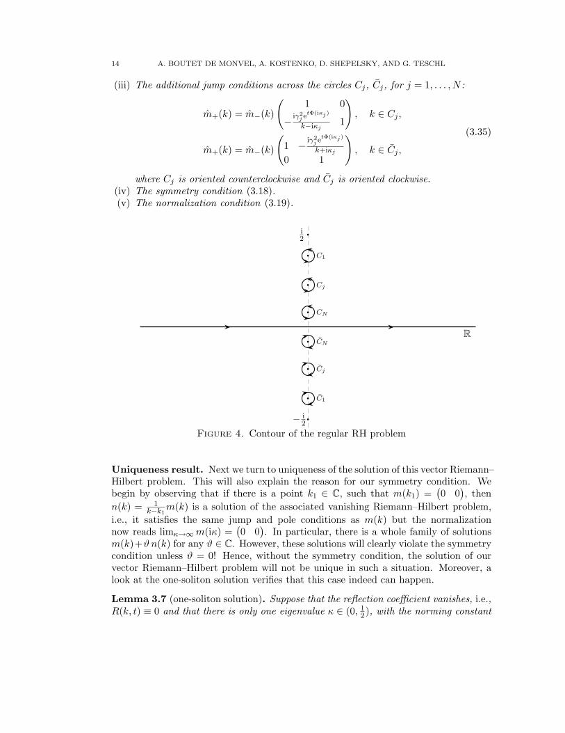
where Cj is oriented counterclockwise and Cj is oriented clockwise.(iv) The symmetry condition (3.18).(v) The normalization condition (3.19).

R

i2

− i2

CNq

Cjq

C1q

q

CNq

Cjq

C1q

q

Figure 4. Contour of the regular RH problem

Uniqueness result. Next we turn to uniqueness of the solution of this vector Riemann–Hilbert problem. This will also explain the reason for our symmetry condition. Webegin by observing that if there is a point k1 ∈ C, such that m(k1) =

(0 0

), then

n(k) = 1k−k1

m(k) is a solution of the associated vanishing Riemann–Hilbert problem,

i.e., it satisfies the same jump and pole conditions as m(k) but the normalizationnow reads limκ→∞ m(iκ) =

(0 0

). In particular, there is a whole family of solutions

m(k)+ϑ n(k) for any ϑ ∈ C. However, these solutions will clearly violate the symmetrycondition unless ϑ = 0! Hence, without the symmetry condition, the solution of ourvector Riemann–Hilbert problem will not be unique in such a situation. Moreover, alook at the one-soliton solution verifies that this case indeed can happen.

Lemma 3.7 (one-soliton solution). Suppose that the reflection coefficient vanishes, i.e.,R(k, t) ≡ 0 and that there is only one eigenvalue κ ∈ (0, 1

2), with the norming constant


γ(t). Then the unique solution of the Riemann–Hilbert problem (3.15)–(3.19) is givenby

m0(k) =(f(k) f(−k)

)(3.36)

f(k) =1

1 + α

(1 + α

k + iκ

k − iκ

),

α =γ2

2κetΦ(iκ).

In particular,

u(x, t) =32κκ2

(1 − 4κ2)2α(y, t)

((1 + α(y, t))2 +

16κ2

1 − 4κ2α(y, t)

)−1

, (3.37)

w(x, t) = κ

(1 +

16κ2

1 − 4κ2

α(y, t)

(1 + α(y, t))2

)2

, (3.38)

where

x = y + log1 + α(y, t)1+2κ

1−2κ

1 + α(y, t)1−2κ1+2κ

. (3.39)

Proof. By assumption the reflection coefficient vanishes and so the jump along the realaxis disappears. Therefore and by the symmetry condition, we know that the solutionis of the form m0(k) =

(f(k) f(−k)

)where f(k) is meromorphic. Furthermore the

function f(k) has only a simple pole at iκ, so that we can make the ansatz f(k) = C +D k+iκ

k−iκ . Then the constants C and D are uniquely determined by the pole conditions and

the normalization. Formulæ (3.37)-(3.38) are obtained applying Lemma 3.5, formula(3.23). ¤

In fact, observe that f(k1) = f(−k1) = 0 if and only if k1 = 0 and 2κ = γ2etΦ(iκ).Furthermore, even in the general case m(k1) =

(0 0

)can only occur at k1 = 0 as the

following lemma shows.

Lemma 3.8. If m(k1) =(0 0

)for m defined as in (3.14), then k1 = 0. Moreover,

the zero of at least one component is simple in this case.

Proof. By (3.14) the condition m(k1) =(0 0

)implies that the Jost solutions ψ−(k, x)

and ψ+(k, x) are linearly dependent or that the transmission coefficient T (k1) = 0.This can only happen at the band edge, k1 = 0 or at an eigenvalue k1 = iκj .

We begin with the case k1 = iκj . In this case the ψ−(k, x) and ψ+(k, x) are linearlydependent. Moreover, T ( · ) has a simple pole at k = k1 since the derivative of theWronskian W(k) = ψ+(k, x)ψ′

−(k, x) − ψ′+(k, x)ψ−(k, x) does not vanish by the well-

known formula

d

dkW(k)|k=k1 = −2k1

κ

∫

R

ψ+(k1, x)ψ−(k1, x)w(x)dx 6= 0

(cf. Lemma 3.2). The diagonal Green’s function g(z, x) = W(k)−1ψ+(k, x)ψ−(k, x) isHerglotz as a function of z = −k2 and hence can have at most a simple zero at z = −k2

1.Since z 7→ −k2 is conformal away from z = 0 the same is true as a function of k. Hence,


if ψ+(iκj , x) = ψ−(iκj , x) = 0, both can have at most a simple zero at k = iκj . ButT (k) has a simple pole at iκj and hence T (k)ψ−(k, x) cannot vanish at k = iκj , acontradiction.

It remains to show that one zero is simple in the case k1 = 0. In fact, one can showthat

d

dkW(k)|k=k1 6= 0

in this case as follows: first of all note that ψ±(k) (where the dot denotes the derivativewith respect to k) again solves

Hψ±(k1) =1

κ

(1

4+ k2

1

)ψ±(k1)

if k1 = 0. Moreover, by W(k1) = 0 we have ψ+(k1) = c ψ−(k1) for some constant c(independent of x). Thus we can compute

W(k1) = W(ψ+(k1), ψ−(k1)) + W(ψ+(k1), ψ−(k1))

= c−1W(ψ+(k1), ψ+(k1)) + c W(ψ−(k1), ψ−(k1))

by letting x → +∞ for the first and x → −∞ for the second Wronskian (in which casewe can replace ψ±(k) by e±ikx), which gives

W(k1) = −i(c + c−1).

Hence the Wronskian has a simple zero. But if both functions had more than simplezeros, so would the Wronskian, a contradiction. ¤

By [20, Theorem 3.2] we obtain

Corollary 3.9. The function m(k, x, t) defined in (3.14) is the only solution of thevector Riemann–Hilbert problem (3.15)–(3.19).

4. Conjugation and Deformation

This section demonstrates how to conjugate our Riemann–Hilbert problem (withrespect to the augmented contour) and how to deform our jump contour, such thatthe jumps will be exponentially close to the identity away from the stationary phasepoints. Throughout this and the following section, we will assume that the R(k) hasan analytic extension to a small neighborhood of the real axis. This is for example thecase if we assume that our solution is exponentially decaying. This assumption canthen be removed using analytic approximation.

For easy reference we note the following result:

Lemma 4.1 (conjugation). Let Σ be a part of some contour Σ. Let D be a matrix ofthe form

D(k) =

(d(k)−1 0

0 d(k)

), (4.1)

where d : C \ Σ → C is a sectionally analytic function. Set

m(k) = m(k)D(k), (4.2)


then the jump matrix transforms according to

v(k) = D−(k)−1v(k)D+(k). (4.3)

If d satisfies d(−k) = d(k)−1 and limk→∞ d(k) = 1, then the transformation

m(k) = m(k)D(k)

respects our symmetry condition, that is, m(k) satisfies (3.18) if and only if m(k) does,and our normalization condition.

In particular, we obtain

v(k) =

(v11 v12d

2

v21d−2 v22

), k ∈ Σ \ Σ,

(d−d+

v11 v12d+d−

v21d−1+ d−1

−d+

d−v22

), k ∈ Σ.

(4.4)

In order to analyse the regular vector RH problem from Lemma 3.6 there are two casesto distinguish.

(a) If Φ(iκj) < 0 then the corresponding jump matrix (3.35) is exponentially close tothe identity as t → +∞ and there is nothing to do.

(b) Otherwise we use conjugation to turn the jumps into one with exponentially de-caying off-diagonal entries.

It turns out that we will have to handle the jumps across Cj and Cj in one step inorder to preserve symmetry and in order to not add additional singularities elsewhere.

Lemma 4.2. Assume that the Riemann–Hilbert problem for m has jump conditionsnear iκ and −iκ given by

m+(k) =

m−(k)

(1 0

− iγ2

k−iκ 1

), |k − iκ| = ε,

m−(k)

(1 − iγ2

k+iκ

0 1

), |k + iκ| = ε.

(4.5)

Then this Riemann–Hilbert problem is equivalent to a Riemann–Hilbert problem form = mD which has jump conditions near iκ and −iκ given by

m+(k) =

m−(k)

(1 − (k+iκ)2

iγ2(k−iκ)

0 1

), |k − iκ| = ε,

m−(k)

(1 0

− (k−iκ)2

iγ2(k+iκ)1

), |k + iκ| = ε,

(4.6)


and all remaining data conjugated by

D(k) =

(1 −k−iκ

iγ2

iγ2

k−iκ 0

) (k−iκk+iκ 0

0 k+iκk−iκ

), |k − iκ| < ε,

(0 − iγ2

k+iκk+iκiγ2 1

) (k−iκk+iκ 0

0 k+iκk−iκ

), |k + iκ| < ε,

(k−iκk+iκ 0

0 k+iκk−iκ

), else.

(4.7)

The jump along the real axis is of oscillatory type and our aim is to apply a contourdeformation following [16] such that all jumps will be moved into regions where theoscillatory terms will decay exponentially. Since the jump matrix v contains bothexp(tΦ) and exp(−tΦ) we need to separate them in order to be able to move them todifferent regions of the complex plane.

We recall that the phase of the associated Riemann–Hilbert problem is given by

Φ(k) = −iκk

14 + k2

+ 2iky

t. (4.8)

Let

c ≡ c(y, t) =y

κt. (4.9)

The stationary phase points, i.e., Φ′(k) = 0, are given by ±k0 and ±k1, where

k0 ≡ k0(c) =1

2

√

−1 + c −√

1 + 4c

c,

k1 ≡ k1(c) =1

2

√

−1 + c +√

1 + 4c

c.

(4.10)

There are four cases to distinguish:

(i) 2κ < yt , i.e. c > 2. In this case

⊲ k0, k1 6∈ R,⊲ Re(Φ) < 0 for Im(k) > 0 near R ∪ i(0, κ0) and⊲ Re(Φ) > 0 for Im(k) > 0 near i(κ0,

12), where

κ0 = 12

√1 − 2

c . (4.11)

We will set κ0 = 0 for yt < 2κ for notational convenience later on.

(ii) 0 < yt < 2κ, i.e. 0 < c < 2. In this case

⊲ k0 ∈ R, k1 6∈ R,⊲ Re(Φ) > 0 for Im(k) > 0 near (−k0, k0) ∪ i(0, 1

2) and⊲ Re(Φ) < 0 for Im(k) > 0 near (−∞,−k0) ∪ (k0,∞).

(iii) −κ

4 < yt < 0, i.e. −1/4 < c < 0. In this case

⊲ k0, k1 ∈ R,⊲ Re(Φ) > 0 for Im(k) > 0 near (−∞,−k1) ∪ (−k0, k0) ∪ (k1,∞) ∪ i(0, 1

2) and⊲ Re(Φ) < 0 for Im(k) > 0 near (−k1,−k0) ∪ (k0, k1).


(iv) yt < −κ

4 , i.e. c < −1/4. In this case⊲ k0, k1 6∈ R and⊲ Re(Φ) > 0 for Im(k) > 0 near R ∪ i(0, 1

2).

The situation is depicted in Figure 5.

c < −1/4

+

−

−+ -

6

............

............

............

............

.............

.............

.............

..........................

.............

.............

.............

............

..

..

..

..

..

..

..

..

..

..

..

..

..

..

..

..

..

..

..

..

..

..

..

..

.

.

.

.

.

.

.

.

.

.

.

.

.

.

.

.

.

.

.

.

.

.

..

..

..

..

.

..

..

..

.

............

......

.........

..........

........

........

.............

............ ............

.............

........

........

..........

.........

......

............

.......

.........

.

.

.

.

.

.

.

.

.

.

.

.

.

.

.

.

.

.

.

.

.

.

............

.

.

.

.

.

.

.

.

.

.

.

..

..

..

..

..

..

..

..

..

..

..

..

..

..

..

..

..

..

..

..

..

..

..

..

............

.............

.............

.............

..........................

.............

.............

.............

............

............

............

............

............

.

.

.

.

.

.

.

.

.

.

.

.

.

.

.

.

.

.

.

.

.

.

.........

.......

............

......

.........

..........

........

........

.............

............ ............

.............

........

........

..........

.........

......

....

........

..

..

..

.

..

..

..

..

.

.

.

.

.

.

.

.

.

.

.

.

−1/4 < c < 0

+

−

−+ -

6

q

k0q

−k0q

k1

q

−k1

.

.

.

.

.

.

.

.

.

.

.

.

.

.

.

.

.

.

.

.

.

.

.

.

.

.

.

.

.

.

.

..

..

..

..

..

.

..

...

....

...

....

...

.

...................

.................

.................

.................

..................

..................

..................................

..................

..................

.................

.................

..

..

..

..

..

..

..

..

.

..

..

..

..

..

..

..

..

..

.

..

..

.

..

..

..

.

..

..

..

.

.

..

..

..

..

..

.

.

.

.

.

.

.

.

.

.

.

.

.

.

.

.

.

.

.

.

.

.

.

.

.

.

.

.

.

.

.

.

.

.

.

.

.

.

.

.

.

.

.

.

.

.

.

.

.

.

.

.

.

.

.

.

.

.

.

.

.

.

.

.

.

.

.

.

.

.

.

.

.

.

.

.

.

.

.

.

.

.

.

.

.

.

.

.

.

.

.

.

.

.

.

.

.

.

.

.

.

.

.

.

.

..

..

..

..

..

.

.

..

..

..

.

..

..

..

.

..

..

.

..

..

..

..

..

..

..

..

..

.

..

..

..

..

..

..

..

..

.

.................

.................

..................

..................

................. .................

..................

..................

.................

.................

.................

...................

..

....

...

....

...

....

.

..

..

..

..

.

.

.

.

.

.

.

.

.

.

.

.

.

.

.

.

.

.

.

.

.

.

.

.

.

.

.

.

.

.

.

.

.

.

.

.

.

.

.

.

.

.

.

.

.

.

.

.

.

.

.

.

.

.

.

.

.

.

.

.

.

.

.

.

.

.

.

.

.

.

.

.

.

.

.

.

..

...

.

.....

..

........

........

........

.........

.........

.........

............................

..........

.........

.........

..

..

.....

..

..

..

..

..

..

..

..

..

..

..

..

..

..

..

.

..

..

.

..

..

.

..

..

..

..

..

.

..

..

..

..

..

..

..

..

..

..

..

..

..

.........

.........

.........

................... .........

..........

.........

.........

.........

........

........

........

..

.....

.

..

..

..

..

0 < c < 2

+

−

−+ -

6

q

k0q

−k0 .......

.

.

.

.

.

.

.

.......

.......

.......

......

.......

.......

.....................

.......

.......

..

..

..

.

......

..

..

..

.

..

..

..

.

..

..

..

.

.

.

.

.

.

.

.

.

.

.

.

.

.

.

.

.

.

.

.

.

.

.

.

.

.

.

.

.

..

..

..

.

..

..

..

.

..

..

..

.

......

..

..

..

.

.......

.............. ..............

.......

.......

......

.......

.......

.......

.

.

.

.

.

.

.

.

.

.

.

.

.

.

2 < c

+

−

-

6

q κ0q−κ0

..

..

.

..

..

..

..

..

..

..

..

.

..........

.....

......

......

.....

.

.....

.....

....

................

..

..

..

..

.

..

..

.

.

.....

......

......

.....

...

.......

..

..

.

..

..

..

..

..

..

..

..

.

.

..

..

.

..

..

.

..

..

................

....

.....

.....

.

Figure 5. Sign of Re(Φ(k)) for different values of c = yκ t

Accordingly we will introduce

Σ(c) =

R, c < −14 ,

(−∞,−k1) ∪ (−k0, k0) ∪ (k1,∞), −14 < c < 0,

(−k0, k0), 0 < c < 2,

∅, 2 < c.

(4.12)

As mentioned above we will need the following factorizations of the jump condition(3.15):

v(k) = b−(k)−1b+(k), (4.13)

where

b−(k) =

(1 R(k)e−tΦ(k)

0 1

), b+(k) =

(1 0

R(k)etΦ(k) 1

). (4.14)

for k ∈ R \ Σ(c) and

v(k) = B−(k)−1

(1 − |R(k)|2 0

0 11−|R(k)|2

)B+(k), (4.15)

where

B−(k) =

(1 0

−R(k)etΦ(k)

1−|R(k)|21

), B+(k) =

(1 −R(k)e−tΦ(k)

1−|R(k)|2

0 1

). (4.16)

for k ∈ Σ(c).To get rid of the diagonal part in the factorization corresponding to k ∈ Σ(c) and to

conjugate the jumps near the eigenvalues we need the partial transmission coefficient


with respect to c defined by

T (k, c) =

∏κ0<κj<1/2

k+iκj

k−iκj, c > 2,

N∏j=1

k+iκj

k−iκjexp

(1

2πi

∫Σ(c)

log(|T (ζ)|2)ζ−k dζ

), c < 2,

(4.17)

for k ∈ C \ Σ(c). Thus T (k, c) is meromorphic for k ∈ C \ Σ(c). Note that T (k, c) canbe computed in terms of the scattering data since |T (k)|2 = 1− |R+(k, t)|2. Moreover,we set

T1(c) = log(T ( i

2 , c))

=

∑κ0<κj<1/2

log1+2κj

1−2κj, c > 2,

N∑j=1

log1+2κj

1−2κj+ 1

π

∫Σ(c)

log(|T (ζ)|2)1+4ζ2 dζ, c < 2.

(4.18)

Note that combining T (k) = eikH−1(w)T (k, c) for c < −14 with (3.33) shows

H−1(w) = 2N∑

j=1

log1 + 2κj

1 − 2κj+

2

π

∫

R

log(|T (ζ)|2)1 + 4ζ2

dζ. (4.19)

Theorem 4.3. The partial transmission coefficient T (k, c) is meromorphic in C \Σ(c)with simple poles at iκj and simple zeros at −iκj for all j with κ0 < κj, and satisfiesthe jump condition

T+(k, c) = T−(k, c)(1 − |R(k)|2), for k ∈ Σ(c). (4.20)

Moreover:

(i) T (−k, c) = T (k, c)−1, k ∈ C \ Σ(c).

(ii) T (−k, c) = T (k, c), k ∈ C, in particular T (k, c) is real for k ∈ iR.(iii) If c < 2 the behaviour near k = 0 is given by T (k, c) = T (k)(C + o(1)) with C 6= 0

for Im(k) ≥ 0.

Proof. That iκj are simple poles and −iκj are simple zeros is obvious from the Blaschkefactors and that T (k, c) has the given jump follows from Plemelj’s formulas. Properties(i), (ii), and (iii) are straightforward to check. ¤

Now we are ready to perform our conjugation step. Introduce

D(k) =

1 − k−iκj

iγ2j etΦ(iκj)

iγ2j etΦ(iκj)

k−iκj0

D0(k), |k − iκj | < ε, κ0 < κj ,

0 − iγ2

j etΦ(iκj)

k+iκjk+iκj

iγ2j etΦ(iκj) 1

D0(k), |k + iκj | < ε, κ0 < κj ,

D0(k), else,

where

D0(k) =

(T (k, c)−1 0

0 T (k, c)

).


Observe that D(k) respects our symmetry:

D(−k) =

(0 11 0

)D(k)

(0 11 0

).

Now we conjugate our problem using D(k) and set

m(k) = m(k)D(k). (4.21)

Note that even though D(k) might be singular at k = 0 (if c < 2 and R(0) = −1), m(k)is nonsingular since the possible singular behaviour of T (k, c)−1 from D0(k) cancelswith T (k) in m(k) by virtue of Theorem 4.3 (iii).

Then using Lemma 4.1 with Σ = Σ(c) and Lemma 4.2 the jump corresponding toκ0 < κj (if any) is given by

v(k) =

(1 − k−iκj

iγ2j etΦ(iκj)T (k,c)−2

0 1

), |k − iκj | = ε,

v(k) =

(1 0

− k+iκj

iγ2j etΦ(iκj)T (k,c)2

1

), |k + iκj | = ε,

(4.22)

and corresponding to κ0 > κj (if any) by

v(k) =

1 0

− iγ2j etΦ(iκj)T (k,c)−2

k−iκj1

, |k − iκj | = ε,

1 − iγ2

j etΦ(iκj)T (k,c)2

k+iκj

0 1

, |k + iκj | = ε.

(4.23)

In particular, all jumps corresponding to poles, except for possibly one if κj = κ0, areexponentially close to the identity. In the latter case we will keep the pole conditionfor κj = κ0 which now reads

Resiκj m(k) = limk→iκj

m(k)

(0 0

iγ2j etΦ(iκj)T (iκj , c)

−2 0

),

Res−iκj m(k) = limk→−iκj

m(k)

(0 −iγ2

j etΦ(iκj)T (iκj , c)−2

0 0

).

(4.24)

Furthermore, the jump along R is given by

v(k) =

{b−(k)−1b+(k), k 6∈ Σ(c),

B−(k)−1B+(k), k ∈ Σ(c),(4.25)

where

b−(k) =

(1 R(−k)e−tΦ(k)

T (−k,c)2

0 1

), b+(k) =

(1 0

R(k)etΦ(k)

T (k,c)21

), (4.26)


and

B−(k) =

(1 0

−T−(k,c)−2

1−|R(k)|2R(k)etΦ(k) 1

)=

(1 0

−T−(−k,c)T−(k,c) R(k)etΦ(k) 1

),

B+(k) =

(1 − T+(k,c)2

1−|R(k)|2R(−k)e−tΦ(k)

0 1

)=

(1 − T+(k,c)

T+(−k,c)R(−k)e−tΦ(k)

0 1

).

Here we have used

R(−k) = R(k), k ∈ R,

T±(−k, c) = T∓(k, c)−1, k ∈ Σ(c),

and the jump condition (4.20) for the partial transmission coefficient T (k, c) along Σ(c)in the last step. This also shows that the matrix entries are bounded for k ∈ R neark = 0 since T±(−k, c) = T±(k, c).

Since we have assumed that R(k) has an analytic continuation to a neighborhood ofthe real axis, we can now deform the jump along R to move the oscillatory terms intoregions where they are decaying.

There are four cases to distinguish:

Case (i): c > 2. We set Σ± = {k ∈ C | Im(k) = ±ε} for some small ε such that Σ±

lies in the region with ±Re(Φ(k)) < 0 and such that the circles Cj , Cj around ±iκj lieoutside the region in between Σ− and Σ+. Then we can split our jump by redefiningm(k) according to

m(k) =

m(k)b+(k)−1, 0 < Im(k) < ε,

m(k)b−(k)−1, −ε < Im(k) < 0,

m(k), else.

(4.27)

Thus the jump along the real axis disappears and the jump along Σ± is given by

v(k) =

{b+(k), k ∈ Σ+

b−(k)−1, k ∈ Σ−.(4.28)

All other jumps are unchanged. By construction the jump along Σ± is exponentiallyclose to the identity as t → ∞.

Cases (ii) and (iii): 0 < c < 2, respectively −1/4 < c < 0. We set Σ± = Σ1± ∪ Σ2

±

according to Figure 6 respectively Figure 7 again such that the circles around ±iκj lieoutside the region in between Σ− and Σ+. Again note that Σ1

± respectively Σ2± lie in

the region with ±Re(Φ(k)) < 0.Then we can split our jump by redefining m(k) according to

m(k) =

m(k)b+(k)−1, k between R and Σ1+,

m(k)b−(k)−1, k between R and Σ1−,

m(k)B+(k)−1, k between R and Σ2+,

m(k)B−(k)−1, k between R and Σ2−,

m(k), else.

(4.29)


One checks that the jump along R disappears and the jump along Σ± is given by

v(k) =

b+(k), k ∈ Σ1+,

b−(k)−1, k ∈ Σ1−,

B+(k), k ∈ Σ2+,

B−(k)−1, k ∈ Σ2−.

(4.30)

All other jumps are unchanged. Again the resulting Riemann–Hilbert problem stillsatisfies our symmetry condition (3.18) and the jump along Σ± \ {±k0,±k1} is expo-nentially decreasing as t → ∞.

Case (iv): c < −1/4. We set Σ± = {k ∈ C | Im(k) = ±ε} for some small ε such thatΣ± lies in the region with ±Re(Φ(k)) > 0 and such that the circles around ±iκj lieoutside the region in between Σ− and Σ+. Then we can split our jump by redefiningm(k) according to

m(k) =

m(k)B+(k)−1, 0 < Im(k) < ε,

m(k)B−(k)−1, −ε < Im(k) < 0,

m(k), else.

(4.31)

Thus the jump along the real axis disappears and the jump along Σ± is given by

v(k) =

{B+(k), k ∈ Σ+

B−(k)−1, k ∈ Σ−.(4.32)

All other jumps are unchanged. By construction the jump along Σ± is exponentiallyclose to the identity as t → ∞.

Note that in all cases the resulting Riemann–Hilbert problem still satisfies our sym-metry condition (3.18), since we have

b±(−k) =

(0 11 0

)b∓(k)

(0 11 0

), B±(−k) =

(0 11 0

)B∓(k)

(0 11 0

). (4.33)

In Cases (i) and (iv) we can immediately apply Theorem A.1 to m as follows:

- -R- - - - -

- - - - -

Σ2− Σ1

− Σ2− Σ1

− Σ2−

Σ2+ Σ1

+ Σ2+ Σ1

+ Σ2+

Re Φ<0

Re Φ>0

Re Φ>0

Re Φ<0Re Φ>0

Re Φ<0Re Φ>0

Re Φ<0

Re Φ<0

Re Φ>0

−k0 k0−k1 k1

.......

.......

........

....

.......

..........

.............

..........

......

....

..

.............

..........

.......

....

........

.......

.............

.......

..

..

..

..

..

..

..

..

..

.

..

..

..

..

..

..

..

..

..

..

..

.

..

..

..

..

..

..

..

..

..

..

..

..

..

..

..

..

..

.

..

..

..

..

..

..

..

..

.

..

..

..

..

..

..

.......

...... .......

.......

........

....

.......

..........

.............

..........

......

....

..

.............

..........

.......

....

........

.......

.............

.......

..

..

..

..

..

..

..

..

..

.

..

..

..

..

..

..

..

..

..

..

..

.

..

..

..

..

..

..

..

..

..

..

..

..

..

..

..

..

..

.

..

..

..

..

..

..

..

..

.

..

..

..

..

..

..

.......

...... .......

.......

........

....

.......

..........

.............

..........

......

....

..

.............

..........

.......

....

........

.......

.............

.......

..

..

..

..

..

..

..

..

..

.

..

..

..

..

..

..

..

..

..

..

..

.

..

..

..

..

..

..

..

..

..

..

..

..

..

..

..

..

..

.

..

..

..

..

..

..

..

..

.

..

..

..

..

..

..

.......

...... .......

.......

........

....

.......

..........

.............

..........

......

....

..

.............

..........

.......

....

........

.......

.............

.......

..

..

..

..

..

..

..

..

..

.

..

..

..

..

..

..

..

..

..

..

..

.

..

..

..

..

..

..

..

..

..

..

..

..

..

..

..

..

..

.

..

..

..

..

..

..

..

..

.

..

..

..

..

..

..

.......

......

.

..

..

.

..

..

.

..

..

.

..

..

.

..

..

.

..

..

.

..

..

.

..

..

.

..

..

.

..

..

.

..

..

.

..

..

.

..

..

.

.

..

..

.

..

..

.

..

..

.

..

..

.

.

.

.

.

.

.

.

.

.

.

.

.

.

.

.

.

.

.

.

.

..

..

.

..

..

.

..

..

.

..

..

.

..

..

.

.

..

..

.

..

..

.

..

..

.

..

..

.

..

..

.

..

..

.

..

..

.

..

..

.

..

..

.

..

..

.

..

..

.

..

..

.

..

..

.

.

..

..

.

..

..

.

..

..

.

..

..

.

..

..

.

..

..

.

..

..

.

..

..

.

..

..

.

..

..

.

..

..

.

..

..

.

..

..

.

.

..

..

.

..

..

.

..

..

.

..

..

.

.

.

.

.

.

.

.

.

.

.

.

.

.

.

.

.

.

.

.

.

..

..

.

..

..

.

..

..

.

..

..

.

..

..

.

.

..

..

.

..

..

.

..

..

.

..

..

.

..

..

.

..

..

.

..

..

.

..

..

.

..

..

.

..

..

.

..

..

.

..

..

.

..

..

.

.

......

.

.

.

.

.

.

.

.

...

.

.

....

....

.

....

.

....

.

....

.

....

.

....

.....

.....

.....

.....

......

.....

.....

.....

.....

.....

..........

................

.........................

...........

.....

.....

.....

.....

.....

.....

.....

.....

.......

..

..

.

..

..

.

..

..

.

..

..

.

..

..

.

..

..

.

..

.

..

.

.

.

.

.

.

.

..

..

..

.

..

..

..

..

..

..

.

.

.

.

.

.

..

.

.

..

.

..

..

.

..

..

.

.

..

..

.

..

..

.

.

..

..

.

..

..

......

.....

......

.....

.....

.....

.....

...........

.....

............... ..... ..... ...........

..... ....................

.....

......

.....

.....

.....

.....

......

.....

.....

.

....

.

....

.

....

.

....

.

....

.

....

.

..

.

...

.

.

.

.

.

.

......

.

....

.

Figure 6. Deformed contour for −1/4 < c < 0


- -R- -

-

Σ1− Σ1

−

Σ2+

.......

.......

........

....

.......

..........

.............

..........

......

....

..

.............

..........

.......

....

........

.......

...... .......

.......

..

..

..

..

..

..

..

..

..

.

..

..

..

..

..

..

..

..

..

..

..

.

..

..

..

..

..

..

..

..

..

..

..

..

..

..

..

..

..

.

..

..

..

..

..

..

..

..

.

..

..

..

..

..

..

.......

......

- -

-

.......

.......

..

..

..

..

..

..

..

..

..

.

..

..

..

..

..

..

..

..

..

..

..

.

..

..

..

..

..

..

..

..

..

..

..

..

..

..

..

..

..

.

..

..

..

..

..

..

..

..

.

..

..

..

..

..

..

.......

...... .......

.......

........

....

.......

..........

.............

..........

......

....

..

.............

..........

.......

....

........

.......

......

Σ1+ Σ1

+

Σ2−

Re Φ>0

Re Φ<0

Re Φ>0

Re Φ<0Re Φ>0

Re Φ<0

−k0 k0.

....

.

....

.

....

.

.

....

.

....

.

....

..

....

.

....

.

....

.

....

.

....

.

....

.

....

.

....

.

....

.....

....

.....

......................

........................

.....

......

....

.

..

..

.

..

..

.

..

..

.

..

..

.

..

..

..

..

..

.

..

..

.

..

..

.

..

..

.

..

..

.

..

..

.

..

..

.

.

..

..

.

..

..

.

..

..

.

.

..

..

.

..

..

.

..

..

.

.

..

..

.

..

..

.

..

..

..

..

..

.

..

..

.

..

..

.

..

..

.

..

..

.

..

..

.

..

..

.

..

..

.

..

..

.....

....

.....

................................

..............

.....

......

....

.

....

.

....

.

....

.

....

.

....

..

....

.

....

.

....

.

....

.

....

.

....

.

....

.

.

....

.

....

.

....

.

Figure 7. Deformed contour for 0 < c < 2

Proof of Theorem 2.1–2.2 (iv). Since v(k) = I + O(t−l) for any l as t → ∞, the sameis true for m(k) =

(1 1

)+ O(t−l) by Theorem A.1 (for the case γ = 0). Hence

m1(k)m2(k) = m1(k)m2(k) = 1 + O(t−l),

m1(i2)

m2(i2)

= e2T1(c) m1(i2)

m2(i2)

= e2T1(c) + O(t−l), (4.34)

for k near i2 and the claim follows from Lemma 3.5 in case the reflection coefficient has

an analytic extensions.Otherwise one has to split the reflection coefficient into an analytic part plus a small

remainder. One can literally follow the argument of [20, Lemma 6.1]. ¤

Proof of Theorem 2.1–2.2 (i). If |xt − cj | > ε for all j we can choose γ = 0 in Theo-rem A.1. Hence as in the proof of (iv),

m1(k)m2(k) = m1(k)m2(k) = 1 + O(t−l),

m1(i2)

m2(i2)

= e2T1(c) m1(i2)

m2(i2)

= e2T1(c) + O(t−l), (4.35)

for k near i2 and the claim follows as before.

Otherwise, if |xt − cj | < ε for some j, we choose γ = γj(x, t). Again we conclude

m1(k)m2(k) = m1(k)m2(k) = f(k)f(−k) + O(t−l),

m1(i2)

m2(i2)

= e2T1(c) m1(i2)

m2(i2)

= e2T1(c) f( i2)

f(− i2)

+ O(t−l), (4.36)

where f(k) is the one-soliton solution from Lemma 3.7. ¤

In the cases (ii) and (iii) the jump will not decay on the small crosses containing thestationary phase points and we need to continue the investigation of this problem inthe next section.


5. Reduction to a Riemann–Hilbert problem on a small cross

In the previous section we have seen that for −1/4 < c < 2 we can reduce everythingto a Riemann–Hilbert problem for m(k) such that the jumps are exponentially closeto the identity except in small neighborhoods of the stationary phase points ±k0 and±k1. Hence we need to continue our investigation of this case in this section.

Denote by Σc(±kℓ), ℓ = 0, 1 the parts of Σ+∪Σ− inside a small neighborhood of ±kℓ.We will now show how to solve the two problems on the small crosses Σc(kℓ) respectivelyΣc(−kℓ) by reducing them to Theorem A.3. This will lead us to the solution of ouroriginal problem by virtue of Theorem A.2.

Now let us turn to the solution of the problem on

Σc(kℓ) = (Σ+ ∪ Σ−) ∩ {k | |k − kℓ| < ε}for some small ε > 0. We can also deform our contour slightly such that Σc(kℓ) consistsof two straight lines. Next, abbreviate

Φℓ = (−1)ℓ Φ(kℓ)

i= −(−1)ℓ 2κk3

ℓ

(1/4 + k2ℓ )

2,

Φ′′ℓ = (−1)ℓ Φ

′′(kℓ)

i= (−1)ℓ 2κkℓ(3/4 − k2

ℓ )

(1/4 + k2ℓ )

3, (5.1)

where Φ′′0 > 0 for −1/4 < c < 2 and Φ′′

1 > 0 for −1/4 < c < 0.As a first step we make a change of coordinates

ζℓ = (−1)ℓ√

Φ′′ℓ (k − kℓ), k = kℓ +

(−1)ℓ

√Φ′′

ℓ

ζℓ (5.2)

such that the phase reads Φ(k) = (−1)ℓ i (Φℓ + 12ζ2 + O(ζ3)).

Next we need the behavior of our jump matrix near kℓ, that is, the behavior of T (k, c)near kℓ.

Lemma 5.1. We have

T (k, c) =

(k−k0k+k0

)iν0(−k−k1

k+k1

)−iν1

T (k, c), −1/4 < c < 0,(

k−k0k+k0

)iν0

T (k, c), 0 < c < 2,(5.3)

where νℓ = − 1π log(|T (kℓ)|) > 0 and the branch cut of the logarithm is chosen along the

negative real axis. Here

T (k, c) =N∏

j=1

k + iκj

k − iκjexp

(− 1

2πi

∫

Σ(c)log(|k − ζ|) d log(|T (ζ)|2)

). (5.4)

The function T ( · , c) is Holder continuous of any exponent less than 1 at the stationary

phase points k = kℓ and satisfies |T (kℓ, c)| = 1.

Proof. This is a straightforward calculation. Holder continuity of any exponent lessthan 1 is well-known (cf. [30]). ¤


If k(ζℓ) is defined as in (5.2) and 0 < α < 1, then there is an L > 0 such that∣∣∣T (k(ζℓ), c) − ζ

(−1)ℓiνℓ

ℓ Tℓ(c)e−(−1)ℓiνℓ log(2kℓ

√Φ′′

ℓ )∣∣∣ ≤ L|ζℓ|α, (5.5)

where the branch cut of ζ iνℓℓ is chosen along the negative real axis and

Tℓ(c) =((−1)ℓ k − kℓ

k + kℓ

)−(−1)ℓiνℓ

T (k, c)∣∣∣k=kℓ

. (5.6)

We also have

|R(k(ζℓ)) − R(kℓ)| ≤ L|ζℓ|α. (5.7)

Set

rℓ = R(kℓ)Tℓ(c)−2e(−1)ℓiνℓ log(4k2

ℓ Φ′′ℓ ) (5.8)

and note νℓ = − 12π log(1 − |R(kℓ)|2) since |rℓ| = |R(kℓ)|. Then the assumptions of

Theorem A.3 are satisfied with r = r0 near for Σc(k0). Similarly, for Σc(k1) they aresatisfied with r = r1 after a conjugation with ( 0 1

1 0 ).Therefore we can conclude that the solution on Σc(kℓ) is given by

M cℓ (k) = I +

1

ζℓ

i

t1/2

(0 −βℓ

βℓ 0

)+ O(t−α)

= I +1√

Φ′′ℓ (k − kℓ)

i

t1/2

(0 −βℓ

βℓ 0

)+ O(t−α), 1/2 < α < 1, (5.9)

where βℓ is given by

β0 =√

νℓei(π/4−arg(r0)+arg(Γ(iν0))−tΦ0)t−iν0

=√

ν0ei(π/4−arg(R(k0))+2 arg(T0(c))−ν0 log(4k2

0Φ′′0 )+arg(Γ(iν0))−tΦ0)t−iν0 , (5.10)

β1 =√

ν1ei(−π/4−arg(r1)−arg(Γ(iν1))+tΦ1)tiν1

=√

νℓei(−π/4−arg(R(k1))+2 arg(T1(c))+ν1 log(4k2

1Φ′′1 )−arg(Γ(iν1))+tΦ1)tiν1 . (5.11)

We also need the solution M cℓ (k) on Σc(−kℓ). We make the following ansatz, which is

inspired by the symmetry condition for the vector Riemann–Hilbert problem, outsidethe two small crosses:

M cℓ (k) =

(0 11 0

)M c

ℓ (−k)

(0 11 0

)

= I − (−1)ℓ

√Φ′′

ℓ (k + kℓ)

i

t1/2

(0 βℓ

−βℓ 0

)+ O(t−α). (5.12)

Now we are ready to finish the proof of Theorem 2.1-2.2.

Proof of Theorem 2.1-2.2 (ii). By Theorem A.2 we infer

m(k) =(1 1

)+

1√Φ′′

0t

i

k − k0

(β0 −β0

)− 1√

Φ′′0t

i

k + k0

(−β0 β0

)

+ O(t−α) (5.13)


and thus

m( i2) =

(1 1

)+

4√Φ′′

0tRe

(β0

1−2ik0− β0

1+2ik0

)+ O(t−α),

m′( i2) =

8i√Φ′′

0tRe

(β0

(1−2ik0)2− β0

(1+2ik0)2

)+ O(t−α). (5.14)

Hence

m1(k)m2(k) =m1(k)m2(k) = 1 − 1√Φ′′

0t

4k0

1/4 + k20

Im(β0) + O(t−α)

−(

1√Φ′′

0t

4k0i

(1/4 + k20)

2Im(β0) + O(t−α)

)(k − i

2) + . . . (5.15)

for k near i2 and Lemma 3.5 implies

w(x, t) = κ − κ√Φ′′

0t

8k0

1/4 + k20

Im(β0) + O(t−α)

u(x, t) = − κ√Φ′′

0t

2k0

(1/4 + k20)

2Im(β0) + O(t−α) (5.16)

Similarly,

m1(i2)

m2(i2)

= e2T1(c) m1(i2)

m2(i2)

= e2T1(c)

(1 +

1√Φ′′

0t

2

1/4 + k20

Re(β0)

)+ O(t−α),

implies

x − y = 2T1(c) +1√Φ′′

0t

2

1/4 + k20

Re(β0) + O(t−α). (5.17)

Thus the claim follows in case the reflection coefficient has an analytic extensions.Otherwise one has to split the reflection coefficient into an analytic part plus a smallremainder using [20, Lem. 6.2 and 6.3]. Again one can literally follow the argumentgiven there. ¤

Proof of Theorem 2.1–2.2 (iii). This follows as in the previous case using

m(k) =(1 1

)+

1√Φ′′

0t

i

k − k0

(β0 −β0

)− 1√

Φ′′0t

i

k + k0

(−β0 β0

)

+1√Φ′′

1t

i

k − k1

(β1 −β1

)− 1√

Φ′′1t

i

k + k1

(−β1 β1

)

+ O(t−α). (5.18)

and hence

w(x, t) = κ − κ√Φ′′

0t

8k0

1/4 + k20

Im(β0) −κ√Φ′′

1t

8k1

1/4 + k21

Im(β1) + O(t−α)

u(x, t) = − κ√Φ′′

0t

2k0

(1/4 + k20)

2Im(β0) −

κ√Φ′′

1t

2k1

(1/4 + k21)

2Im(β1) + O(t−α) (5.19)


respectively

x − y = 2T1(c) +1√Φ′′

0t

2

1/4 + k20

Re(β0) +1√Φ′′

1t

2

1/4 + k21

Re(β1) + O(t−α). (5.20)

¤

Appendix A. Some results for Riemann–Hilbert problems

In this section we state the results required to prove or main theorems. We willassume that Σ is a nice contour, say a finite number of smooth oriented finite curves inC, which intersect at most finitely many times with all intersections being transversal.Moreover, suppose the distance between Σ and {iy | y ≥ y0} is positive for some y0 > 0.

A.1. Riemann–Hilbert problem for the soliton region. The first result is neededin the soliton region. Consider the Riemann–Hilbert problem of finding a function m(k)satisfying

(i) m(k) is sectionally meromorphic with simple poles at ±iκ 6∈ Σ,(ii) the jump condition

m+(k) = m−(k)v(k), k ∈ Σ,

(iii) the pole condition

Resiκ m(k) = limk→iκ

m(k)

(0 0

iγ2 0

),

(iv) the symmetry condition

m(−k) = m(k)

(0 11 0

),

(v) the normalization condition

limk→∞

m(k) =(1 1

).

Clearly the symmetry condition implies that our jump data (Σ, v) should be symmetricas well, that is,

v(−k) =

(0 11 0

)v(k)−1

(0 11 0

), k ∈ Σ. (A.1)

and Σ is invariant under k 7→ −k and oriented such that under the mapping k 7→ −ksequences converging from the positive sided to Σ are mapped to sequences convergingto the negative side. Moreover (ii) and (iii) imply

Res−iκ m(k) = limk→−iκ

m(k)

(0 −iγ2

0 0

).

Finally we will assume ‖v − I‖2 < ∞ and ‖v − I‖∞ < ∞.We are interested in comparing this Riemann–Hilbert problem with the one-soliton

problem (where v ≡ 0) in the case where ‖v − I‖∞ and ‖v − I‖2 are small. For such asituation we have the following result:


Theorem A.1 ([20, 24]). Assume v = v(t) satisfies

‖v(t) − I‖∞ ≤ ρ(t),

‖v(t) − I‖2 ≤ ρ(t)(A.2)

for some function ρ(t) → 0 as t → ∞. Then the above Riemann–Hilbert problem hasa unique solution for sufficiently large t and the solution differs from the one-solitonsolution by O(ρ(t)) uniformly in k away from Σ ∪ {±iκ}.

A.2. Riemann–Hilbert problem for oscillatory regions. For the oscillatory re-gions we will need the following result which allows us to reduce everything to a modelproblem whose solution will be given below.

Theorem A.2 ([20, 24]). Consider the vector Riemann–Hilbert problem

m+(k) = m−(k)v(k), k ∈ Σ,

limk→∞

m(k) =(1 1

),

(A.3)

with det(v) 6= 0 and let 0 < α < β ≤ 2α, ρ(t) → ∞ be given.Suppose that for every sufficiently small ε > 0 both the L2 and the L∞ norms of

v are O(t−β) away from some ε neighborhoods of some points ki ∈ Σ, 1 ≤ i ≤ n.Moreover, suppose that the solution of the matrix problem with jump v(k) restricted tothe ε neighborhood of ki has a solution which satisfies

Mi(k) = I +1

ρ(t)α

Mi

k − ki+ O(ρ(t)−β), |k − ki| > ε. (A.4)

Then the solution m(k) is given by

m(k) =(1 1

)+

1

ρ(t)α

(1 1

) n∑

i=1

Mi

k − ki+ O

(ρ(t)−β

), (A.5)

where the error term depends on the distance of k to Σ.

Model problem on a cross. Introduce the cross Σ = Σ1 ∪ · · · ∪Σ4 (see Figure 8) by

Σ1 = {ue−iπ/4 | u ≥ 0}, Σ2 = {ueiπ/4 | u ≥ 0},Σ3 = {ue3iπ/4 | u ≥ 0}, Σ4 = {ue−3iπ/4 | u ≥ 0}.

(A.6)

Orient Σ such that the real part of k increases in the positive direction. Denote byD = {ζ ∈ C | |ζ| < 1} the open unit disc. Throughout this section ζ iν will denote the

function eiν log(ζ), where the branch cut of the logarithm is chosen along the negativereal axis (−∞, 0).

Introduce the following jump matrices (vj for ζ ∈ Σj , j = 1, . . . , 4)

v1 =

(1 −R1(ζ)ζ2iνe−tΦ(ζ)

0 1

), v2 =

(1 0

R2(ζ)ζ−2iνetΦ(ζ) 1

),

v3 =

(1 −R3(ζ)ζ2iνe−tΦ(ζ)

0 1

), v4 =

(1 0

R4(ζ)ζ−2iνetΦ(ζ) 1

) (A.7)


@@

@@

@@

@@

@@

@@

@@@

@@R

@@R

¡¡

¡¡

¡¡

¡¡

¡¡

¡¡

¡¡¡

¡¡µ

¡¡µ

Σ1

Σ2Σ3

Σ4

(1 −R1(ζ) · · ·0 1

)

(1 0

R2(ζ) · · · 1

)

(1 −R3(ζ) · · ·0 1

)

(1 0

R4(ζ) · · · 1

)

Figure 8. Contours of a cross

and consider the RHP given by

M+(ζ) = M−(ζ)vj(ζ), ζ ∈ Σj , j = 1, 2, 3, 4, (A.8)

M(ζ) → I, ζ → ∞.

The solution is given in the following theorem of P. Deift and X. Zhou [16, Sect. 3-4](for a proof of the version stated below see H. Kruger and G. Teschl [25, Theorem A.1]).

Theorem A.3 ([16]). Assume there is some ρ0 > 0 such that vj(ζ) = I for |ζ| > ρ0

and j = 1, . . . , 4. Moreover, suppose that within |ζ| ≤ ρ0 the following estimates hold:

(i) The phase satisfies Φ(0) = iΦ0 ∈ iR, Φ′(0) = 0, Φ′′(0) = i, and

± Re(Φ(ζ)

)≥ 1

4|ζ|2, with

{+ for ζ ∈ Σ1 ∪ Σ3,

− else,(A.9)

∣∣∣Φ(ζ) − Φ(0) − iζ2

2

∣∣∣ ≤ C|ζ|3. (A.10)

(ii) There is some r ∈ D and constants (α, L) ∈ (0, 1] × (0,∞) such that R1, . . . , R4

satisfy Holder conditions of the form

|R1(ζ) − r| ≤ L|ζ|α, |R2(ζ) − r| ≤ L|ζ|α,∣∣∣∣R3(ζ) − r

1 − |r|2∣∣∣∣ ≤ L|ζ|α,

∣∣∣∣R4(ζ) − r

1 − |r|2∣∣∣∣ ≤ L|ζ|α.

(A.11)

Then the solution of the RHP (A.8) satisfies

M(k) = I +1

ζ

i

t1/2

(0 −β

β 0

)+ O(t−

1+α2 ), (A.12)

for |ζ| > ρ0, where

β =√

ν ei(π/4−arg(r)+arg(Γ(iν)))e−itΦ0t−iν , ν = − 1

2πlog(1 − |r|2). (A.13)


Furthermore, if Rj(ζ) and Φ(ζ) depend on some parameter, the error term is uniformwith respect to this parameter as long as r remains within a compact subset of D andthe constants in the above estimates can be chosen independent of the parameters.

Acknowledgments. We are indebted to Ira Egorova for helpful discussions on varioustopics of this paper and to Adrian Constantin for comments on a previous version ofthis article. One of us (A. K.) gratefully acknowledges financial support from theInternational Erwin Schrodinger Institute for Mathematical Physics in the form of ajunior fellowship during which parts of this research were done.

References

[1] A. Boutet de Monvel, A. Its, and D. Shepelsky, Painleve-type asymptotics for the

Camassa–Holm equation, preprint, 2009.[2] A. Boutet de Monvel and D. Shepelsky, The Camassa–Holm equation on the half-line, C.

R. Math. Acad. Sci. Paris 341 (2005), pp. 611–616.[3] A. Boutet de Monvel and D. Shepelsky, Riemann–Hilbert approach for the Camassa–Holm

equation on the line, C. R. Math. Acad. Sci. Paris 343 (2006), pp. 627–632.[4] A. Boutet de Monvel and D. Shepelsky, Riemann–Hilbert problem in the inverse scattering

for the Camassa–Holm equation on the line, in “Probability, Geometry and Integrable Systems”,53–75, Math. Sci. Res. Inst. Publ. 55, Cambridge Univ. Press, Cambridge, 2008.

[5] A. Boutet de Monvel and D. Shepelsky, Long-time asymptotics of the Camassa–Holm

equation on the line, in “Integrable Systems and Random Matrices: In honor of Percy Deift”,Baik et al. (eds), 99–116, Contemporary Mathematics 458, Amer. Math. Soc., Providence,2008.

[6] A. Boutet de Monvel and D. Shepelsky, The Camassa–Holm equation on the half-line: a

Riemann–Hilbert approach, J. Geom. Anal. 18 (2008), pp. 285–323.[7] R. Camassa and D. Holm, An integrable shallow water equation with peaked solitons, Phys.

Rev. Letters 71 (1993), pp. 1661–1664.[8] R. Camassa, D. Holm, and J. M. Hyman, A new integrable shallow water equation, Adv.

Appl. Mech. 31 (1994), pp. 1–33.[9] A. Constantin, On the scattering problem for the Camassa–Holm equation, Proc. R. Soc.

Lond. A 457 (2001), pp. 953–970.[10] A. Constantin and J. Escher, Global existence and blow-up for a shallow water equation,

Annali Sc. Norm. Sup. Pisa 26 (1998), pp. 303–328.[11] A. Constantin, V. S. Gerdjikov, and R. I. Ivanov, Inverse scattering transform for the

Camassa–Holm equation, Inverse Problems 22 (2006), pp. 2197–2207.[12] A. Constantin and D. Lannes, The hydrodynamical relevance of the Camassa-Holm and

Degasperis–Procesi equations, Arch. Rational Mech. Anal. 192 (2009), pp. 165–186.[13] A. Constantin and J. Lenells, On the inverse scattering approach for an integrable shallow

water equation, Phys. Lett. A 308 (2003), pp. 432–436.[14] A. Constantin and W. Strauss, Stability of peakons, Comm. Pure Appl. Math. 53 (2000),

pp. 603–610.[15] P. Deift and E. Trubowitz, Inverse scattering on the line, Commun. Pure Appl. Math. 32

(1979), pp. 121–251.[16] P. Deift and X. Zhou, A steepest descent method for oscillatory Riemann–Hilbert problems,

Ann. of Math. (2) 137 (1993), pp. 295–368.[17] P. A. Deift, A. R. Its, A. R., and X. Zhou, Long-time asymptotics for integrable non-

linear wave equations, in “Important developments in soliton theory”, 181–204, Springer Ser.Nonlinear Dynam., Springer, Berlin, 1993.

[18] K. El Dika and L. Molinet, Stability of multipeakons, Ann. Inst. H. Poincare Anal. NonLineaire, to appear.


[19] B. Fuchssteiner and A. Fokas, Symplectic structures, their Backlund transforms and hered-

itary symmetries, Phys. D 4 (1981), pp. 47–66.[20] K. Grunert and G. Teschl, Long-time asymptotics for the Korteweg–de Vries equation via

nonlinear steepest descent, arXiv:0807.5041.[21] A. R. Its, Asymptotic behavior of the solutions to the nonlinear Schrodinger equation, and

isomonodromic deformations of systems of linear differential equations, Soviet. Math. Dokl. 24(1981), pp. 452–456.

[22] R. S. Johnson, Camassa–Holm, Korteweg–de Vries and related models for water waves, J.Fluid Mech. 455 (2002), pp. 63–82.

[23] R. S. Johnson, On solutions of the Camassa–Holm equation, Proc. R. Soc. London, Ser. A 459(2003), pp. 1687–1708.

[24] H. Kruger and G. Teschl, Long-time asymptotics for the Toda lattice in the soliton region,Math. Z., 262 (2009), pp. 585–602.

[25] H. Kruger and G. Teschl, Long-time asymptotics of the Toda lattice for decaying initial data

revisited, Rev. Math. Phys. 21 (2009), pp. 61–109.[26] L.-C. Li, Long time behaviour for a class of low-regularity solutions of the Camassa–Holm

equation, Comm. Math. Phys. 285 (2009), pp. 265–291.[27] S. V. Manakov, Nonlinear Frauenhofer diffraction, Sov. Phys. JETP 38 (1974) pp. 693–696.[28] V. A. Marchenko, Sturm–Liouville Operators and Applications, Birkhauser, Basel, 1986.[29] Y. Matsuno, Parametric representation for the multisoliton solution of the Camassa–Holm

equation, J. Phys. Soc. Jpn. 74 (2005), pp. 1983–1987.[30] N. I. Muskhelishvili, Singular Integral Equations, P. Noordhoff Ltd., Groningen, 1953.

Institut de Mathematiques de Jussieu, Universite Paris Diderot Paris 7, 175 rue du

Chevaleret, 75013 Paris, France

E-mail address: [email protected]

URL: http://www.math.jussieu.fr/~aboutet/

Institute of Applied Mathematics and Mechanics, NAS of Ukraine, R. Luxemburg str.

74, Donetsk 83114, Ukraine


B.Verkin Institute for Low Temperature Physics, 47 Lenin Avenue, 61103 Kharkiv,

Ukraine


Faculty of Mathematics, Nordbergstrasse 15, 1090 Wien, Austria, and International

Erwin Schrodinger Institute for Mathematical Physics, Boltzmanngasse 9, 1090 Wien,

Austria


URL: http://www.mat.univie.ac.at/~gerald/

http://arxiv.org/abs/0807.5041

mailto:[email protected]

http://www.math.jussieu.fr/~aboutet/




http://www.mat.univie.ac.at/~gerald/

· long-time asymptotics for the camassa–holm equation anne boutet de monvel, aleksey kostenko,...

Documents