geosynthetics engineering: in theory and … 23.pdf · geosynthetics engineering: in theory and...

GEOSYNTHETICS ENGINEERING: IN THEORY AND PRACTICE

Prof. J. N. Mandal

Department of civil engineering, IIT Bombay, Powai , Mumbai 400076, India. Tel.022-25767328email: [email protected]

Prof. J. N. Mandal, Department of Civil Engineering, IIT Bombay

Module-5LECTURE- 23

GEOSYNTHETICS IN PAVEMENTS



RECAP of previous lecture…..

Stress reduction downwards with depth of granular fill

Advantages of unpaved roads

Design charts of U.S. forest service (USFS) for

unpaved roads

U.S. forest service design curves

Modified California bearing ratio (CBR) test

Design of pavement thickness without geogrid (IRC37)

Design of Reinforced Unpaved road (Giroud and Han, 2004)

r = radius of equivalent tire contact area (m),

P = wheel load in kN, and

p = tire contact pressure; (kPa).

Step 1: Calculate the radius of the equivalent contact areausing following equation.

pPr


Step 2: Calculate the California Bearing Ration of thesub-grade soil or undrained cohesion of sub-grade soil,

cu = undrained cohesion of sub-grade soil

fC = factor equal to 30kPa

C.B.Rsg = sub-grade California bearing ratio (< 5)

sgcu CBRfc

Step 3: Calculate the allowable bearing capacity of sub-grade soil without reinforcement.

sgcc2

suc

2

sorcedinfunre,0h CBRfNr

fscNr

fsP


s = Allowable rut depth is equal to 40 mm,

f S = factor equal to 75 mm,

r = radius of the equivalent tire contact area,

Nc = bearing capacity factor equal to 3.14,

cu = undrained cohesion of subgrade soil, and

CBRsg = subgrade California bearing ratio

If the wheel load is greater than the allowable bearingcapacity of subgrade soil, a base course is required withoutor with geosynthetics.


Step 4: Determine the limit modulus ratio (RE) and modulusratio factor (fE).

Ebc = base course resilient modulus,

Esg = subgrade resilient modulus,

CBRbc = base course California bearing ratio, and

CBRsg = subgrade California bearing ratio,

0.5,)CBR(48.3min0.5,EEminR 3.0

bcsg

bcE

Modulus ratio factor, fE = 1 + 0.204 (RE - 1)

To calculate the base course thickness, the following stepsshould be followed.


Step 5: Determine the bearing capacity mobilizationcoefficient (m) in term of thickness (h).

2

( ) 1 0.9 exps

s rmf h

m = bearing capacity mobilization coefficient,

s = allowable rut depth (mm)

50 < s < 100 (as per Giroud, 2004)

f S = factor equal to 75 mm

r = radius of equivalent tire contact area (m), and

h = thickness of base course.Prof. J. N. Mandal, Department of Civil Engineering, IIT Bombay

Step 6: Determine the require base course thickness

2 1.520.868 (0.661 1.006 )( ) log / 1

E c c sg

rJ N P rhh rf mN f CBR

J = aperture stability modulus of geogrid (mN/ ) (< 0.8) ,

J = 0 for geotextile and in unreinforced case

h = thickness of required base course (m),

P = wheel load (kN), and

Nc = bearing capacity factor = 5.71 (for geogrid)

Nc, geotextile= 5.14, Nc, unreinforced = 3.14

Calculation of the base course thickness needs iterations.Prof. J. N. Mandal, Department of Civil Engineering, IIT Bombay

If the calculated ‘h’ value does not match the assumed ‘h’value, ‘m’ value is to be recalculated and is used as theassumed value for the next iteration. The process is to berepeated until the calculated value is approximately equal toassumed value.

Step 7: Determine the reduction in base course thicknessusing geogrid or geotextile (h) = h0 – h

Let, h0 = thickness of required base course for unreinforcedcase (m)

h = thickness of required base course with geogrid orgeotextile (m)


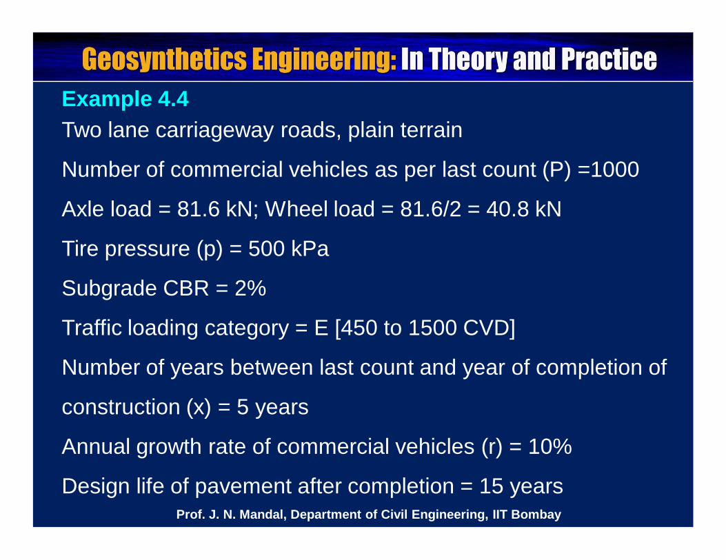
Example 4.4Two lane carriageway roads, plain terrain

Number of commercial vehicles as per last count (P) =1000

Axle load = 81.6 kN; Wheel load = 81.6/2 = 40.8 kN

Tire pressure (p) = 500 kPa

Subgrade CBR = 2%

Traffic loading category = E [450 to 1500 CVD]

Number of years between last count and year of completion of

construction (x) = 5 years

Annual growth rate of commercial vehicles (r) = 10%

Design life of pavement after completion = 15 yearsProf. J. N. Mandal, Department of Civil Engineering, IIT Bombay

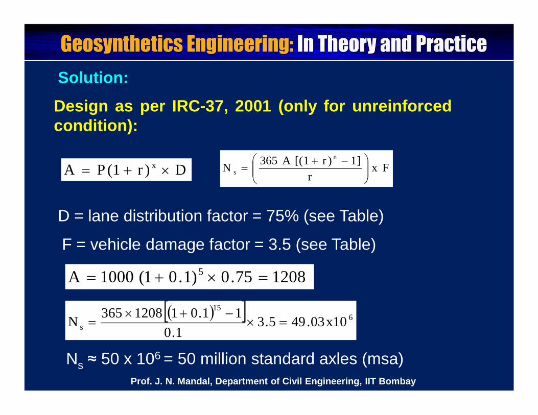
Solution:

D)r1(PA x Fxr

]1)r1[(A365Nn

s

F = vehicle damage factor = 3.5 (see Table)

D = lane distribution factor = 75% (see Table)

Design as per IRC-37, 2001 (only for unreinforcedcondition):

615

s 10x03.495.31.0

11.011208365N

120875.0)1.01(1000A 5

Ns ≈ 50 x 106 = 50 million standard axles (msa)Prof. J. N. Mandal, Department of Civil Engineering, IIT Bombay

From design chart, for 2% CBR and 50 msa standard axle,Total pavement thickness = 925 mm = 0.925 m

Design Chart for determining pavement thickness, traffic 10-150 msa (IRC-37, 2001)


Pavement composition (Reference from IRC 37):

Cross- section of Pavement

Bituminous surfacing = 21.5 cm[Bituminous Concrete (B.C.) = 4 cmBituminous Macadam (D.B.M.) = 17.5 cm]


Design as per Giroud and Han, 2004 (without and withreinforcement):

Input data ValuesAxle load (kN), Q 135Wheel load (kN), P 67.5Tire pressure (kPa), p 500Radius of the equivalent tire contact area (m), r 0.207Base course C.B.R. (%), C.B.R.bc 20C.B.R. of the subgrade soil (%), C.B.R.sg 2Allowable rut depth (mm), s 40Factor (kPa), fc 30Factor (kPa), fs 75Geogrid aperture stability modulus (m N/o), J 0.65Number of axle passes, N 50 x 106

Bearing capacity factor, Nc, unreinforced 3.14Nc, geogrid 5.71Nc, geotextile 5.14


Output User InterfaceFor unpaved road in unreinforced condition:Assumed

base course thickness, hassumed (m)

0.3 1.11 0.82 0.88 0.86 0.87 FINISHED #VALUE!

1. Limited modulus ratio, RE

4.274

2. Modulus ratio factor, fE

1.668

3. Bearing capacity mobilization factor, m

0.235 0.069 0.083 0.079 0.080 0.079 #VALUE! #VALUE!

Required base course thickness,

hfinal (m)

1.11 0.82 0.88 0.86 0.87 0.87 #VALUE! #VALUE!


For unpaved road with geogrid:

Assumed base course thickness, hassumed (m)

0.3 0.35 0.37 FINISHED #VALUE!


4.27


1.67

3. Bearing capacity mobilization factor, m 0.235 0.195 0.182 #VALUE! #VALUE!

Required base course thickness, hfinal (m)

0.35 0.37 0.37 #VALUE! #VALUE!


Assumed base course thickness, hassumed (m)

0.3 0.77 0.65 0.67 FINISHED #VALUE!


4.274


1.667

3. Bearing capacity mobilization factor, m

0.235 0.086 0.099 0.097 #VALUE! #VALUE!

Required base course thickness, hfinal (m)

0.77 0.65 0.67 0.67 #VALUE! #VALUE!

For unpaved road with geotextile:


For geogrid reinforced unpaved road, a factor of safety isconsidered = 1.5Percentage of saving (%):

Thickness of base course for unreinforced unpaved road (mm), hunreinforced

870 mm

Thickness of base course with geogrid (mm), hgeogrid

370 x 1.5 = 555 mm

Thickness of base course with geotextile (mm), hgeotextile

670 mm

% Saving (geogrid) 36.21%

% Saving (geotextile) 23%Prof. J. N. Mandal, Department of Civil Engineering, IIT Bombay

Geogrid and geocomposite layers are to be provided inbetween subgrade and sub-base layers.

The geocomposite layer will drain out the infiltrated waterfrom base course and the uplifted water from subgrade.

Base course thickness using geogrid = 55.5 cm ≈ 56 cm

Pavement composition (Geogrid reinforced):Bituminous surfacing (Reference to IRC: 37) = 21.5 cmsurfacing consisting of 4 cm bituminous concrete (B.C.) and17.5 cm dense bituminous macadam (D.B.M.)

Base course: 20 cm Water Bound Macadam (W.B.M) (20 %C.B.R.)

Sub-base: 35 cm granular material of CBR not less than 30%Prof. J. N. Mandal, Department of Civil Engineering, IIT Bombay

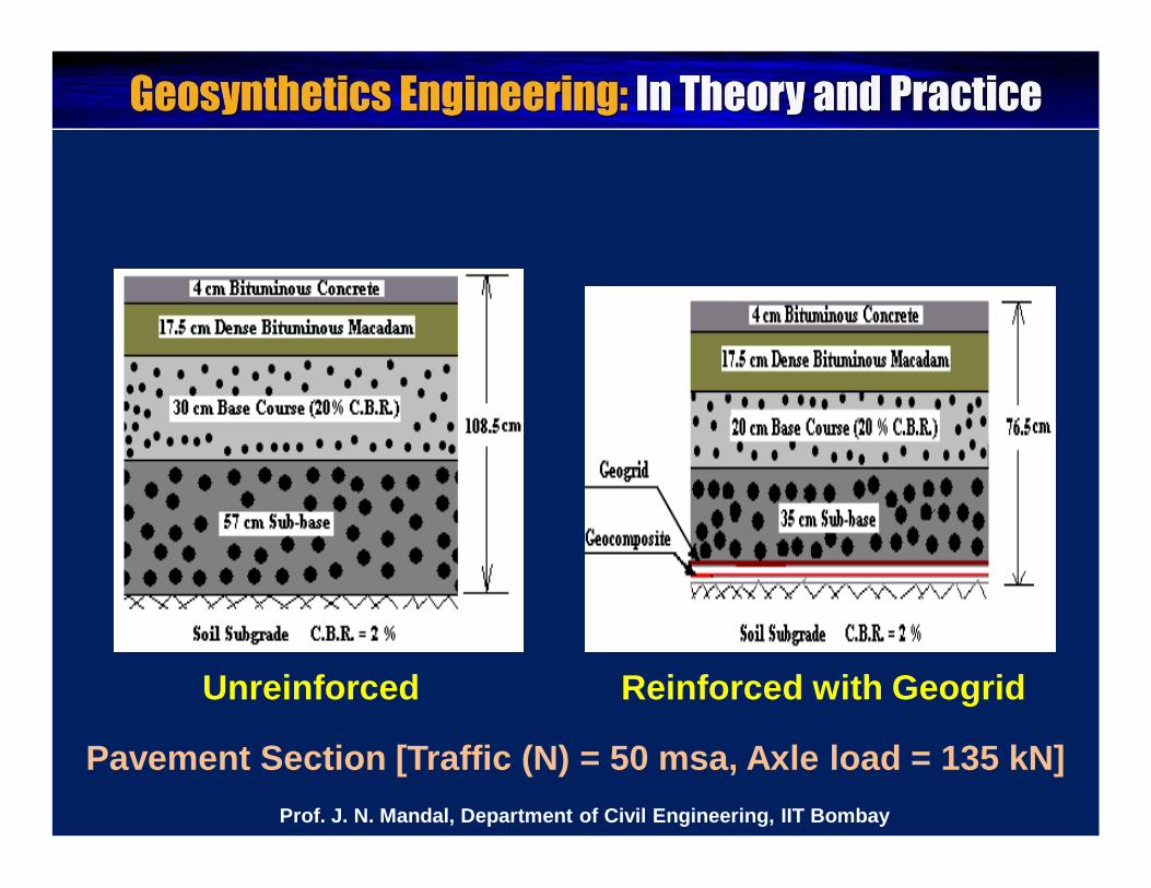
Pavement Section [Traffic (N) = 50 msa, Axle load = 135 kN]

Unreinforced Reinforced with Geogrid


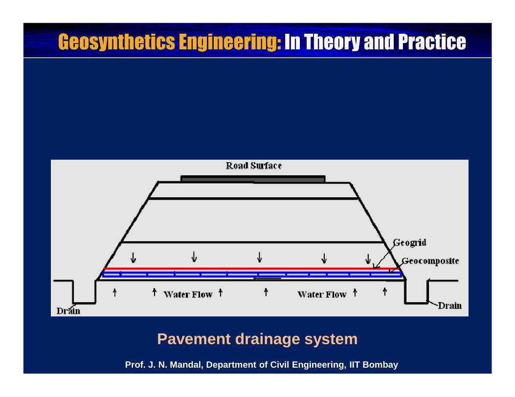
Pavement drainage systemProf. J. N. Mandal, Department of Civil Engineering, IIT Bombay

0

125

250

375

0 125 250 375 500 625

Equ

ival

ent r

einf

orce

d ba

se

thic

knes

s (m

m)

Nonreinforced base thickness (mm)

Geogrid at midpoint of base layer

Geogrid at bottom of base layer

Geogrid reinforced base course for paved highway (Carroll et al. 1987)

At 250 mm geogrid can be introduced either at the bottom or in the middle of the base course for specific geogrid


AASHTO (1993) Design Method for Flexible Pavement

Design problem: A flexible pavement for a road (2 laneseach direction) needs to be designed for 25-years life. Average sub-grade CBR = 2% Expected traffic: tandem axle 36 kips, 100,000/year. Noannual growth rate to be considered. Terminal serviceability, pt = 2.5

Reliability level (R) = 95%; standard deviation, So = 0.35 Asphalt layer coefficient (a1) = 0.40, base course layercoefficient, (a2) = 0.14, sub-base layer coefficient (a3) = 0.08. Drainage condition is “Good”; pavement is exposed tosaturation moisture more than 25% of the time.


Solution:

Without reinforcement:

Step 1: Determination of W18

(a) For tandem axle 36 kips, pt =2.5 and assumed SN of 6.0, the axle load equivalency factor = 1.38 (From Table I)

Hence, first year traffic estimate

= Expected traffic x axle load equivalency factor

= 100,000 x 1.38 = 138,000

W18 = predicted number of 18,000 lb equivalent single axleload (ESAL) applications


(b) For analysis period of 25 years and no growth,

traffic growth factor = 25 (From Table II)

Hence,

w’18 = Traffic growth factor x First year traffic estimate

= 25 x 138,000 = 3,450,000

Table I Axle load equivalency factors for flexible pavements,tandem axles and pt = 2.5 (AASTHO, 1993)

Axle load

(kips)

Axle load equivalency factor

Pavement Structural Number (SN)

1 2 3 4 5 624 0.231 0.273 0.315 0.292 0.260 0.24226 0.327 0.370 0.420 0.401 0.364 0.34228 0.451 0.493 0.548 0.534 0.495 0.47030 0.611 0.648 0.703 0.695 0.658 0.63332 0.813 0.843 0.889 0.887 0.857 0.83434 1.06 1.08 1.11 1.11 1.09 1.0836 1.38 1.38 1.38 1.38 1.38 1.3838 1.75 1.73 1.69 1.68 1.70 1.7340 2.21 2.16 2.06 2.03 2.08 2.14


Analysis period(years)

Traffic growth factor

Annual Growth Rate, Percent

No growth 2 4 5 6 7 8 10

15 15 17.29 20.02 21.58 23.28 25.13 27.15 31.77

20 20 24.30 29.78 33.07 36.79 41.00 45.76 57.27

25 25 32.03 41.65 47.73 54.86 63.25 73.11 98.35

30 30 40.57 56.08 66.44 79,06 94.46 113.28 164.49

35 35 49.99 73.65 90.32 111.43 138.24 172.32 271.02

Table II Traffic growth factor (AASTHO, 1993)


(c) Generally for most roadways, DD = 0.5

DD = a directional distribution factor

From Table III, DL = 0.90 (two lanes in each direction)

Hence, w18 = DD x DL x w’18

= 0.50 x 0.90 x 3,450,000

= 1,552,500


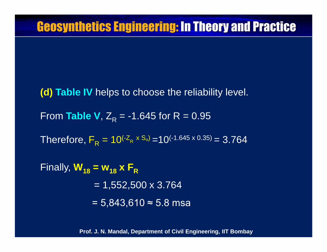
(d) Table IV helps to choose the reliability level.

From Table V, ZR = -1.645 for R = 0.95

Therefore, FR = 10(-ZR x So) =10(-1.645 x 0.35) = 3.764

Finally, W18 = w18 x FR

= 1,552,500 x 3.764

= 5,843,610 ≈ 5.8 msa


Number of Lanes in Each Direction

Percent of ESAL in Design Lane (DL)

1 1002 80-1003 60-804 50-75

Table III Lane Distribution Factor, DL (AASTHO, 1993)


Table IV Suggested Levels of Reliability (AASTHO, 1993)

Functional Classification

Recommended Level of Reliability (R)

Urban Rural

Interstate and Other Freeways 85-99.9 80-99.9

Principal Arterials 80-99 75-95

Collector 80-95 75-95

Local 50-80 50-80


Reliability (%) ZR

50 0.00060 -0.25370 -0.52485 -0.84190 -1.28295 -1.64599 -2.327

99.9 -3.090

Table V Standard normal deviate for different values ofreliability, R


Step 2: Determination of serviceability

Given pt =2.5; po = 4.2 (if not given)

po = Initial design serviceability index

∆PSI = po - pt = 4.2 - 2.5 = 1.7

Step 3: Determination of subgrade Resilient Modulus (MR)

MR (psi) = 1,500 x CBR = 1,500 x 2 = 3000 psi

MR (kPa) = 6.89 x 1500 x CBR= 6.89 x 1500 x 2= 20670 kPa


Step 4: Determination of Structural Number (SN)

Basic empirical equation for design of flexible pavement byAmerican Association of State Highway and Transportation(AASHTO, 1993) is as follows (in FPS units).

07.8)M(log32.2

1SN109440.0

5.12.4PSIlog

20.0)1SN(log36.9S.Z)W(log R10

19.5

10

10oR1810

Determine the structural number (SN) by trial and errormethod or use the design charts given.

Here, W18 = 5843610, ZR = -1.645, So = 0.35, ∆PSI = 1.7 and MR = 3000 psi

Therefore, SN = 6.16 Prof. J. N. Mandal, Department of Civil Engineering, IIT Bombay

Design chart of CBR vs. SN for 1 to 10 msa (R = 95 % and So= 0.35)


Step 5: Estimation of pavement thicknessFor unreinforced case,

SN = a1.D1 + a2.D2.m2 + a3.D3.m3

D1, D2 and D3 = thickness (in inches) of the surface, base and sub-base respectively

a1, a2, a3 = structural layer coefficients for the surface, base and sub-base respectively (The layer coefficients depend upon the resilient modulus of the material.)

m2, m3 = drainage coefficient for base course and sub-base course respectively

As SN value has already been determined in step 4, D1, D2and D3 can be obtained by trial and error.


(a) Generally, the typical layer coefficients used by AASTHOroad test are as follows:a1 = Asphalt concrete surface course = 0.40-0.44,a2 = Crushed stone base course = 0.10-0.14, anda3 = Sandy graved sub-base = 0.060-0.11

We obtain a1 = 0.40, a2 = 0.14, a3 = 0.08 (given)

(b) Drainage: Modified layer coefficients are used to accountfor the improved drainage conditions. The quality of drainageand recommended drainage coefficients can be obtainedfrom Tables VI and VII respectively.As the drainage condition is “Good” and pavement isexposed to saturation moisture more than 25% of the time,m2 = 1.0 and m3 = 1.0


Quality of Drainage Duration of Water Removal

Excellent 2 hours

Good 1 day

Fair 1 week

Poor 1 month

Very poor Water will not drain

Table VI Drainage Conditions (AASTHO, 1993)


Table VII Recommended mi Values (as per AASTHO, 1993)

Quality of

Drainage

Recommended mi ValuePercent of Time Pavement is Exposed to Moisture Levels Approaching Saturation<1% 1-5% 2-25% >25%

Excellent 1.40-1.35 1.35-1.30 1.30-1.20 1.20Good 1.35-1.25 1.25-1.15 1.15-1.00 1.0Fair 1.25-1.15 1.15-1.05 1.00-0.80 0.80Poor 1.15-1.05 1.05-0.80 0.80-0.60 0.60Very Poor 1.05-0.95 0.95-0.75 0.75-0.40 0.40


We have already calculated by trial and error, SN = 6.16

6.16 = 0.40.D1 + 0.14.D2.1+ 0.08. D3.1

or, 6.16 = 0.40 D1 + 0.14.D2 + 0.08 .D3

Assuming surface layer depth (D1) = 0.21 m

Assuming base course depth (D2) = 0.25 m

Hence, sub-base depth (D3) = 0.47 m

Total thickness = (0.21 + 0.25 + 0.47) = 0.93 m Prof. J. N. Mandal, Department of Civil Engineering, IIT Bombay

Step 6: Design for Reinforced Case

For reinforced case we know that,

SN = a1.D1 + a2.D2.m2 + (LCR).a3.D3.m3

(N.B. D1, D2 and D3 are in inches)

a1 = 0.40, a2 = 0.14, a3 = 0.08 (given)

m2 = 1.0 and m3 = 1.0

LCR value depends on CBR of subgrade and types ofreinforcement used.


Here, LCR = 1.4 for CBR = 2


Already calculated, SN = 6.16

6.16 = 0.40 x D1 + 0.14 x D2 x 1+1.4 x 0.08 x D3 x 1

or, 6.16 = 0.40 D1 + 0.14.D2 + 0.112.D3

Assuming surface Layer Depth (D1) = 0.21 m

Assuming base course Depth (D2) = 0.25 m

Hence, sub-base Course Depth (D3) = 0.33 m

Total thickness = (0.21 + 0.25 + 0.33) = 0.79 m


100depth subbase edunreinforc

depth subbasereinforced -depth subbaseedunreinforc Saving%

%57.281000.47

0.33-0.47Saving%

Step 7: Saving of sub-base course material (%)


Pavement Design without and with Geosynthetics (W18 = 5.8 msa)


Please let us hear from you

Any question?


Prof. J. N. Mandal

Department of civil engineering, IIT Bombay, Powai , Mumbai 400076, India. Tel.022-25767328email: [email protected]


geosynthetics engineering: in theory and … 23.pdf · geosynthetics engineering: in theory and...

Documents