geostatistical reservoir characterization of the canyon ... library/research/oil-gas/enhanced...
TRANSCRIPT
Topical Report Geostatistical Reservoir Characterization of the Canyon Formation, SACROC Unit, Permian Basin September, 2007 Performed by: Reinaldo J. Gonzalez and Scott R. Reeves Advanced Resources International, Inc. 11490 Westheimer Rd., Suite 520 Houston, TX 77077 Prepared for: U.S. Department of Energy Contract No. DE-FC26-04NT15514
SACROC GEOSTATISTICAL SP091407
i
Disclaimers
U.S. Department of Energy This report was prepared as an account of work sponsored by an agency of the United States Government. Neither the United States Government nor any agency thereof, nor any of their employees, makes any warranty, express or implied, or assumes any legal liability or responsibility for the accuracy, completeness, or usefulness of any information, apparatus, product, or process disclosed, or represents that its use would not infringe privately owned rights. Reference herein to any specific commercial product, process, or service by trade name, trademark, manufacturer, or otherwise does not necessarily constitute or imply its endorsement, recommendation, or favoring by the United States Government or any agency thereof. The views and opinions of authors expressed herein do not necessarily state or reflect those of the United States Government or any agency thereof.
Advanced Resources International, Inc.
The material in this Report is intended for general information only. Any use of this material in relation to any specific application should be based on independent examination and verification of its unrestricted applicability for such use and on a determination of suitability for the application by professionally qualified personnel. No license under any Advanced Resources International, Inc., patents or other proprietary interest is implied by the publication of this Report. Those making use of or relying upon the material assume all risks and liability arising from such use or reliance.
SACROC GEOSTATISTICAL SP091407
ii
Executive Summary
Accurate, high-resolution, three-dimensional (3D) reservoir characterization can provide substantial benefits for effective oilfield management. By doing so, the predictive reliability of reservoir flow models, which are routinely used as the basis for significant investment decisions designed to recover millions of barrels of oil, can be substantially improved. This is particularly true when Secondary Oil Recovery (SOR) or Enhanced Oil Recovery (EOR) operations are planned. If injectants such as water, hydrocarbon gasses, steam, CO2, etc. are to be used; an understanding of fluid migration paths can mean the difference between economic success and failure. SOR/EOR projects will increasingly take place in heterogeneous reservoirs where interwell complexity is high and difficult to understand. The industry therefore needs improved reservoir characterization approaches that are quicker, more accurate, and less expensive than today’s standard methods.
To achieve this objective, the Department of Energy (DOE) has been promoting some
studies with the goal of evaluating whether robust relationships between data at vastly different scales of measurement could be established using advanced pattern recognition (soft computing) methods. Advanced Resources International (ARI) has performed two of these projects with encouraging results showing the feasibility of establishing critical relationships between data at different measurement scales to create high-resolution reservoir characterization.
In this third study performed by ARI and also funded by the DOE, a model-based,
probabilistic clustering analysis procedure is successfully applied to generate a high-resolution reservoir characterization outcome. The approach was applied in the Pennsylvanian-Permian reef carbonates (Cisco and Canyon Formations) of a subregion of the SACROC Unit, Horseshoe Atoll, Permian Basin, Texas, and acknowledged as a highly complex carbonate reservoir.
A selected area within the SACROC Unit platform was used for this study. A two-step
“soft-computing” procedure was developed in the first stage of the project for efficiently generating core-scale porosity and permeability values (as well as rock types geologically consistent) at well locations where only gamma ray (GR) and neutron porosity logs (NPHI) were available. In this way, “core” parameter profiles, with high vertical resolution, could be generated for many wells which permitted to populate any well location with core-scale estimates of porosity and permeability (P&P) and rock types facilitating direct application of geostatistical methods to build 3D reservoir models.
This process provided a data set of twenty two (22) wells in the study area with foot-by-
foot profiles of P&P, and was considered to be sufficient information to characterize directly the reservoir distributions of P&P. Next, stochastic simulation algorithms were utilized to provide reservoir models of P&P in the selected study region with different levels of vertical resolution.
This report is focused on the application of geostatistical methods for the reservoir
characterization at SACROC. We present results derived from variogram analyses applied to P&P (actual and pseudo data), and rock types at well locations. These results were utilized to
SACROC GEOSTATISTICAL SP091407
iii
model the spatial variability of parameters P&P through variography studies using directly the vertical profiles of core P&P set on each subregion well. Once the corresponding models of spatial continuity of P&P were established, the stochastic simulation algorithm known as Sequential Gaussian Simulation (SGS) was utilized to generate the final reservoir models of porosity and permeability in the selected study area.
Different scales of variability were seen in variograms of core P&P in the reef-carbonate
depositional environment of SACROC. The vertical variogram analysis indicated spatial behaviors associated with geologic cyclicity; however, cyclicity could not be appreciated in the horizontal variogram analyses. Both variography studies, vertical and horizontal, conducted to variogram models using an isotropic nugget structure and two structures with geometric anisotropy reflecting an intermediate and a global scale. These different scales were mainly associated to complex patterns of sediment deposition of the reservoir, and constructional characteristics of the SACROC limestone reef (structural factors).
The P&P characterizations were developed in a grid that could work directly in the flow
simulator. In consequence, the geostatistical characterizations and posterior reservoir flow simulations were both conducted on the same Cartesian grid. A direct application of SGS algorithms to actual and estimate values of core P&P lead to 3D models of porosity and permeability that honored the raw data and honored quite closely the division of the carbonate section into "good" and "poor" reservoir quality (RQ) zones.
From the qualitative and quantitative point of views, a porosity model highly trustworthy
was developed with this combined methodology (average porosity of this heterogeneous model was 8.5%). On the other hand, a highly reliable permeability model was generated from the qualitative viewpoint (identification and characterization of geological trends and realistic heterogeneities); however, estimated permeability values were considered possibly undervalued (average horizontal permeability of the model was 2.74 mD). This fact is attributable to the smoothing effect inherent to algorithms based on Gaussian assumptions.
The direct application of conventional geostatistical algorithms in this work was favored
by the considerable quantity of information present on wells inside the studied region. This definitively was a consequence of the application of advanced pattern recognition techniques that provided likely rock types and reliable estimates of P&P (with high vertical resolution) at all well locations. Reciprocally, the utilization of geostatistical algorithms allowed the three-dimensional extension, of those results derived from the application of the clustering methodology, to the whole volume of the area under study. This “symbiotic” interaction between these two mathematical approaches strengthens their corresponding possibilities of applicability offering a significant advance over their individual uses, and other conventional methodologies.
This combined approach -application of advanced pattern recognition techniques and
geostatistical algorithms- has the potential of being successfully applied either on other subregions of SACROC or entirely on the whole SACROC unit.

SACROC GEOSTATISTICAL SP091407
iv
Table of Contents Disclaimers...................................................................................................................................... i
Executive Summary...................................................................................................................... ii
List of Tables ................................................................................................................................. v
List of Figures............................................................................................................................... vi
1.0 Introduction....................................................................................................................... 1
2.0 Geostatistical Approach ................................................................................................... 8
3.0 Stratigraphic Coordinate System .................................................................................... 9
4.0 Variogram Analysis ........................................................................................................ 11
4.1 Methodology ................................................................................................................. 11
4.2 SACROC Variography.................................................................................................. 13
4.3 Porosity Variography.................................................................................................... 16
4.4 Permeability Variography ............................................................................................ 21
4.5 Cross-Variogram Analysis............................................................................................ 27
4.6 Rock Type Variography ................................................................................................ 30
5.0 Grid Definition ................................................................................................................ 38
6.0 Sequential Gaussian Simulation .................................................................................... 40
6.1 Porosity Model.............................................................................................................. 41
6.2 Permeability Model....................................................................................................... 43
6.3 Results ........................................................................................................................... 47
6.4 Supplementary Considerations of Implementation....................................................... 52
7.0 Conclusions...................................................................................................................... 57
8.0 References........................................................................................................................ 59
9.0 List of Acronyms and Abbreviations ............................................................................ 60
SACROC GEOSTATISTICAL SP091407
v
List of Tables Table 1: Parameter Values for Horizontal Geometric Anisotropy of Normalized Porosity ....................... 19 Table 2: Correlation Coefficients for Different Window-Averaged Values............................................... 25 Table 3: Correlation Coefficients for 15 and 112 Foot Grid Blocks........................................................... 25 Table 4: Summary of Parameter Values Describing the Horizontal Geometric Anisotropy of Normalized
Permeability ................................................................................................................................... 27 Table 5: Reformulation of Original Rock Types ........................................................................................ 30 Table 6: Statistical Summary of Porosity Simulated Values ...................................................................... 42 Table 7: Statistical Summary Of Permeability Simulated Values .............................................................. 45
SACROC GEOSTATISTICAL SP091407
vi
List of Figures Figure 1: Pathway to 3D High-Resolution Reservoir Description................................................................ 2 Figure 2: Illustration of Different Scales of Measurement ........................................................................... 3 Figure 3: Schematic of the Two-Step “Soft-Computing” Procedure............................................................ 6 Figure 4: SACROC Field and Study Area (Test Site) .................................................................................. 7 Figure 5: Directional “Wedge” and Utilized Parameters for 2D Variogram Analysis. .............................. 16 Figure 6: Vertical Experimental Variogram of Normalized Porosity ......................................................... 17 Figure 7: Directional Experimental Variograms of Normalized Porosity .................................................. 18 Figure 8: Superimposed Anisotropy Ellipses Describing the Nested Scales of the Porosity Spatial
Variability ...................................................................................................................................... 20
Figure 9: Experimental and Model Variograms of Normalized Porosity at N0°E ..................................... 20
Figure 10: Experimental and Model Variograms of Normalized Porosity at N45°E ................................. 21 Figure 11: Experimental Vertical Variogram of Normalized Log10(K0).................................................... 22 Figure 12: Extended Vertical Variogram of Normalized Log10(K0) .......................................................... 22 Figure 13: Extended Vertical Variogram of the Normalized Porosity........................................................ 23 Figure 14: Vertical Experimental Variogram of Normalized Log10(K0) with a Theoretical Model Fit ..... 23 Figure 15: Directional Experimental Variograms of Normalized Log10(K0). ............................................ 24
Directions: 0°, 30°, 45°, 60°, 90°, 120°, 135°, and 150° ............................................................................ 24 Figure 16: Window Averaged Permeability (Logarithm) and Porosity...................................................... 26 Figure 17: Cross Vertical Experimental Variogram Between Normalized Porosity and Normalized
Log10(K0)....................................................................................................................................... 28 Figure 18: Cross Vertical Model Variogram Between Normalized Porosity and Normalized Log10(K0) .28 Figure 19: Eight Directional Experimental Cross Variograms of Normalized Porosity and Normalized
Log10(K0). ...................................................................................................................................... 29 Figure 20: Modeled Cross Variograms of Normalized Porosity and Normalized Log10(K0). ................... 30 Figure 21: Experimental Vertical Variograms of Regrouped Rock Types 1, 2, 3, 4 .................................. 31 Figure 22: Variogram Model of Regrouped Rock Type 2.......................................................................... 32 Figure 23: Variogram Model of Regrouped Rock Type 3.......................................................................... 32 Figure 24: Experimental Variograms of Original Rock Types 3, 5, and 10 (Good Limestone) ................. 33 Figure 25: Experimental Variograms of Original Rock Types 4, 6, and 9 (Shale)..................................... 33 Figure 26: Variogram Models Fit to Experimental Variograms of Original Modes 3, 5, and 10 (Good
Limestone) ..................................................................................................................................... 34
SACROC GEOSTATISTICAL SP091407
vii
Figure 27: Directional Experimental Variograms of Regrouped Rock Types 1, 2, 3, and 4. Directions 0°,
45°, 90° and 135° ........................................................................................................................... 35
Figure 28: Directional Experimental Variograms of Original Rock Type 3. Directions 0°, 45°, 90° and
135°................................................................................................................................................ 36
Figure 29: Directional Experimental Variograms of Original Rock Type 5. Directions 0°, 45°, 90° and
135°................................................................................................................................................ 36
Figure 30: Directional Experimental Variograms of Original Rock Type 10. Directions 0°, 45°, 90° and
135°................................................................................................................................................ 36 Figure 31: Study Area with Planned Cross-Well Surveys & CO2 Injection Pattern................................... 38 Figure 32: Study Area Location, SACROC Unit - Northern Platform ....................................................... 39 Figure 33: Four Different Realizations of Porosity Generated by SGS Algorithm .................................... 41 Figure 34: Wells with Porosity Values and Grid Frame (left), Geostatistical Porosity Model (right) ....... 42 Figure 35: Histogram of Porosity Simulated Values (“Average” Porosity Model) .................................... 43 Figure 36: Wells with Log10(K0) Values and Grid Frame (left), Geostatistical Model of Log10(K0) (right)
....................................................................................................................................................... 44 Figure 37: Wells with Permeability Values (K0) and Grid Frame (left), Geostatistical Permeability Model
(K0) (right)..................................................................................................................................... 44 Figure 38: Histogram of Permeability Simulated Values ........................................................................... 45 Figure 39: Simulated Values of Permeability vs. Simulated Values of Porosity: Logarithm of Permeability
(left), Permeability (right).............................................................................................................. 46 Figure 40: Location of Cross Sections A-A’, B-B’, and C-C’.................................................................... 47 Figure 41: Cross Section C-C’ (left) and Cross Section A-A’ (right) Showing Rock Types Probabilistic
Representation ............................................................................................................................... 48
Figure 42: Porosity and Permeability Cross Sections N° 20 and N° 11 ..................................................... 49
Figure 43: Magnified View of Cross Section N° 11 - Porosity at Left, Permeability at Right................... 50
Figure 44: Magnified View of Cross Section N° 20 - Porosity at Left, Permeability at Right................... 50
Figure 45: Permeability Indicator Maps, Cut-Off = 2.74 md, Cross Section N° 11 at Left (N-S), Cross
Section N° 20 at Right (E-W) ........................................................................................................ 50
Figure 46: XY Areal Sections N° 4, N° 22 and N° 45 of Porosity at Left, Permeability at Right.............. 51 Figure 47: Omnidirectional Experimental Variogram of Normalized Top Depth...................................... 53 Figure 48: Model Generated for Top Depth of the Canyon Reef ............................................................... 53 (depth in feet).............................................................................................................................................. 53

SACROC GEOSTATISTICAL SP091407
viii
Figure 49: Areal XY Section N°25 of the Porosity Model Displayed Using Graphic Tools of Simulator
IMEX (Porosity is in Fractions)..................................................................................................... 54
Figure 50: N-S Cross Section N° 16 of Porosity 3D Model ....................................................................... 55
Figure 51: E-W Cross Section N° 16 of Porosity 3D Model ...................................................................... 55 Figure 52: 3D General View of the Porosity Model (Porosity is in Fractions) .......................................... 56
SACROC GEOSTATISTICAL SP091407
1
1.0 Introduction
Accurate, high-resolution, three-dimensional (3D) reservoir characterization can provide substantial benefits for effective oilfield management. By doing so, the predictive reliability of reservoir flow models, which are routinely used as the basis for significant investment decisions designed to recover millions of barrels of oil, can be substantially improved. Even a small improvement in incremental oil recovery for high-value assets can result in important contributions to bottom-line profitability.
This is particularly true when Secondary Oil Recovery (SOR) or Enhanced Oil Recovery
(EOR) operations are planned. If injectants such as water, hydrocarbon gasses, steam, CO2, etc. are to be used; an understanding of fluid migration paths can mean the difference between economic success and failure. In these types of projects, injectant costs can be a significant part of operating expenses, and hence their optimized utility is critical.
SOR/EOR projects will increasingly take place in heterogeneous reservoirs where
interwell complexity is high and difficult to understand. Although reasonable reservoir characterization information often exists at the wellbore, the only economical way to sample the interwell region is with seismic methods. Surface reflection seismic has relatively low cost per unit volume of reservoir investigated, but the resolution of surface seismic data available today, particularly in the vertical dimension, is not sufficient to produce the kind of detailed reservoir description necessary for effective SOR/EOR optimization and planning.
Today’s standard practice for developing a 3D reservoir description is to use seismic
inversion techniques. These techniques make use of rock physics concepts to solve the inverse problem, i.e., to iteratively construct a likely geologic model and then upscale and compare its acoustic response to that actually observed in the field. This method suffers from the fact that rock physics relationships are not well understood, and the need to rely on porosity-permeability transforms to estimate permeability from porosity. Further, these methods require considerable resources to perform, and thus it is applied to only a small percentage of oil and gas producing assets.
Since the majority of fields do not utilize these technologies currently, many fields are
sub-optimally developed. The industry therefore needs an improved reservoir characterization approach that is quicker, more accurate, and less expensive than today’s standard methods. This will permit more reservoirs to be better characterized, allowing recoveries to be optimized and significantly adding to recoverable reserves.
A new approach to achieve this objective was first examined in a Department of Energy
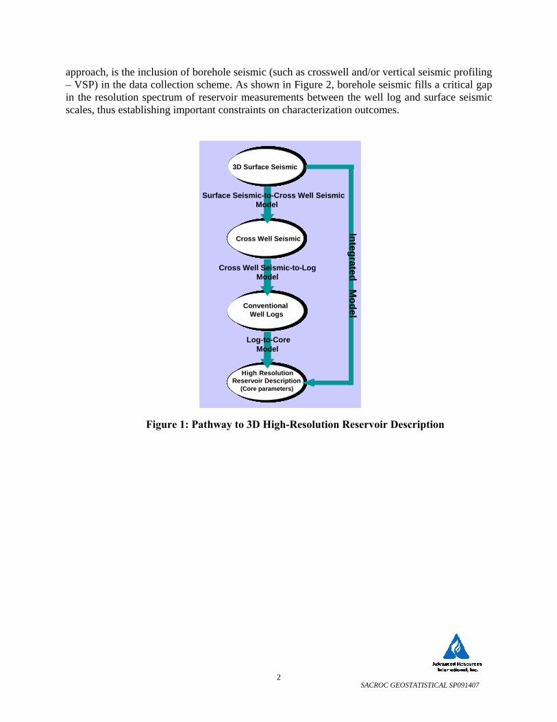
(DOE) study performed by Advanced Resources International (ARI) in 2000/20011. The goal of that study was to evaluate whether robust relationships between data at vastly different scales of measurement could be established using virtual intelligence (VI) methods. The proposed workflow required that three specific relationships be established through use of data-driven modeling methods, in that case artificial neural networks (ANN’s): core-to-log, log-to-crosswell seismic, and crosswell-to-surface seismic as shown in Figure 1. One of the key attributes of the
SACROC GEOSTATISTICAL SP091407
2
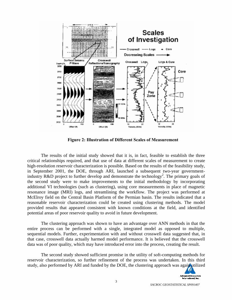
approach, is the inclusion of borehole seismic (such as crosswell and/or vertical seismic profiling – VSP) in the data collection scheme. As shown in Figure 2, borehole seismic fills a critical gap in the resolution spectrum of reservoir measurements between the well log and surface seismic scales, thus establishing important constraints on characterization outcomes.
Figure 1: Pathway to 3D High-Resolution Reservoir Description
Borehole Seismic
(X - Well, VSP)
Borehole Seismic
(X - Well, VSP)
Borehole Seismic
(X - Well, VSP)Cross Well SeismicBorehole Seismic
(X - Well, VSP)
Borehole Seismic
(X - Well, VSP)
Borehole Seismic
(X - Well, VSP)Cross Well Seismic
3 - D Surface Seismic3 -D Surface Seismic3 - D Surface Seismic3D Surface Seismic3 - D Surface Seismic3 -D Surface Seismic3 - D Surface Seismic3D Surface Seismic
Conventional Well LogsConventional Well LogsConventional Well LogsConventional Well Logs
Conventional Well LogsConventional Well LogsConventional Well LogsConventional Well Logs
High - Resolution
Reservoir Description
(Core, MRI, etc.)
High - Resolution
Reservoir Description
(Core, MRI, etc.)
High - Resolution
Reservoir Description
(Core, MRI, etc.)
High ResolutionReservoir Description
(Core parameters)
High - Resolution
Reservoir Description
(Core, MRI, etc.)
High - Resolution
Reservoir Description
(Core, MRI, etc.)
High - Resolution
Reservoir Description
(Core, MRI, etc.)
High ResolutionReservoir Description
(Core parameters)
Surface Seismic-to-Cross Well SeismicModel
Cross Well Seismic-to-LogModel
Log-to-CoreModel
Integrated Model
Borehole Seismic
(X - Well, VSP)
Borehole Seismic
(X - Well, VSP)
Borehole Seismic
(X - Well, VSP)Cross Well SeismicBorehole Seismic
(X - Well, VSP)
Borehole Seismic
(X - Well, VSP)
Borehole Seismic
(X - Well, VSP)Cross Well Seismic
3 - D Surface Seismic3 -D Surface Seismic3 - D Surface Seismic3D Surface Seismic3 - D Surface Seismic3 -D Surface Seismic3 - D Surface Seismic3D Surface Seismic
Conventional Well LogsConventional Well LogsConventional Well LogsConventional Well Logs
Conventional Well LogsConventional Well LogsConventional Well LogsConventional Well Logs
High - Resolution
Reservoir Description
(Core, MRI, etc.)
High - Resolution
Reservoir Description
(Core, MRI, etc.)
High - Resolution
Reservoir Description
(Core, MRI, etc.)
High ResolutionReservoir Description
(Core parameters)
High - Resolution
Reservoir Description
(Core, MRI, etc.)
High - Resolution
Reservoir Description
(Core, MRI, etc.)
High - Resolution
Reservoir Description
(Core, MRI, etc.)
High ResolutionReservoir Description
(Core parameters)
Surface Seismic-to-Cross Well SeismicModel
Cross Well Seismic-to-LogModel
Log-to-CoreModel
Integrated Model
SACROC GEOSTATISTICAL SP091407
3
Figure 2: Illustration of Different Scales of Measurement The results of the initial study showed that it is, in fact, feasible to establish the three
critical relationships required, and that use of data at different scales of measurement to create high-resolution reservoir characterization is possible. Based on the results of the feasibility study, in September 2001, the DOE, through ARI, launched a subsequent two-year government-industry R&D project to further develop and demonstrate the technology2. The primary goals of the second study were to make improvements to the initial methodology by incorporating additional VI technologies (such as clustering), using core measurements in place of magnetic resonance image (MRI) logs, and streamlining the workflow. The project was performed at McElroy field on the Central Basin Platform of the Permian basin. The results indicated that a reasonable reservoir characterization could be created using clustering methods. The model provided results that appeared consistent with known conditions at the field, and identified potential areas of poor reservoir quality to avoid in future development.
The clustering approach was shown to have an advantage over ANN methods in that the
entire process can be performed with a single, integrated model as opposed to multiple, sequential models. Further, experimentation with and without crosswell data suggested that, in that case, crosswell data actually harmed model performance. It is believed that the crosswell data was of poor quality, which may have introduced error into the process, creating the result.
The second study showed sufficient promise in the utility of soft-computing methods for
reservoir characterization, so further refinement of the process was undertaken. In this third study, also performed by ARI and funded by the DOE, the clustering approach was again utilized
SACROC GEOSTATISTICAL SP091407
4
to generate a high-resolution reservoir characterization outcome as the first step in an integrated Clustering/Geostatistical approach for 3D Reservoir Characterization. The entire study, the subject of a previous report3 and this report, was performed at the SACROC Unit, operated by Kinder Morgan (KMCO2), in the Permian basin of West Texas.
As discussed in the first topical report3, the heart of the original procedure was to create
three data-driven devices (or eventually an integrated one) capable of utilizing the raw data, as well as the clustering information, to relate
• Surface to crosswell seismic (specifically seismic attributes to crosswell traces). • Crosswell attributes (computed from crosswell traces) to geophysical log responses. • Geophysical logs to core permeability and porosity.
These data types should be explored and conditioned, individually and in combination,
using clustering techniques to identify patterns and commonalities in data. With these three “intelligent” devices or models (Figure 1), any surface seismic trace could be deconvolved from a low-resolution elastic waveform to a high-resolution representation of porosity and permeability (P&P), which would permit the development of a model capable of predicting core-scale porosity and permeability profiles even in locations where only 3D surface seismic data is available.
Due to successive postponements on the execution of crosswell survey and therefore the
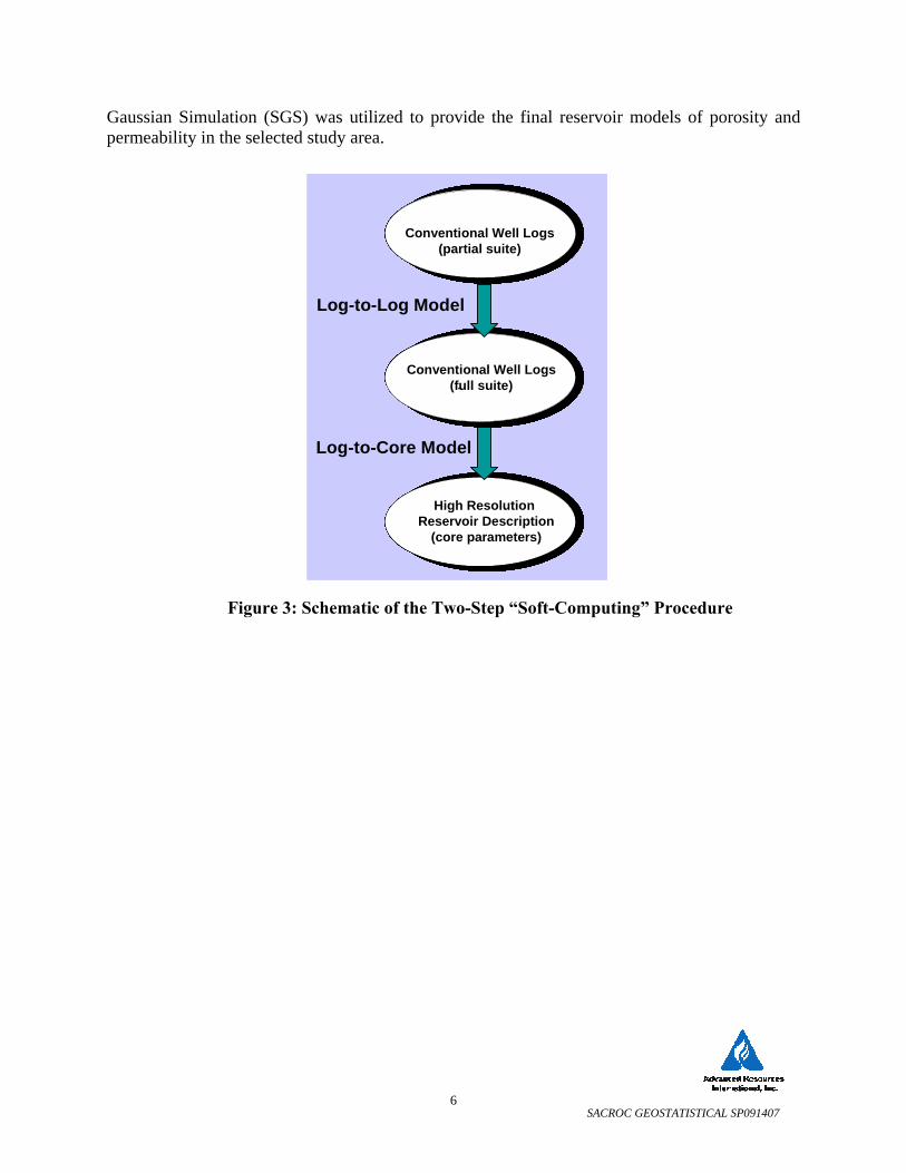
absence of crosswell data, the characterization process was commenced with the available information, consisting of core data, well logs information and 3D surface seismic data. As a product of these efforts, a two-step “soft-computing” procedure was developed capable of efficiently generating core-scale porosity and permeability values (as well as rock types geologically consistent) at well locations where only gamma ray (GR) and neutron porosity logs (NPHI) were available. These are the most common logs for wells in this reservoir. All detailed results are shown in the original topical report3. Because the suitable logs for the creation of a direct Log-to-Core “intelligent” device were not present at all wells, it was necessary to create another intelligence tool, a Log-to-Log model, to provide missing information. The ideal suite of well logs considered for the characterization tasks was constituted by bulk density (RHOB), delta time (DT), GR, and NPHI. Figure 3 illustrates schematically this two-step procedure. The validity of these soft-computing devices was checked using "holdout" wells3.
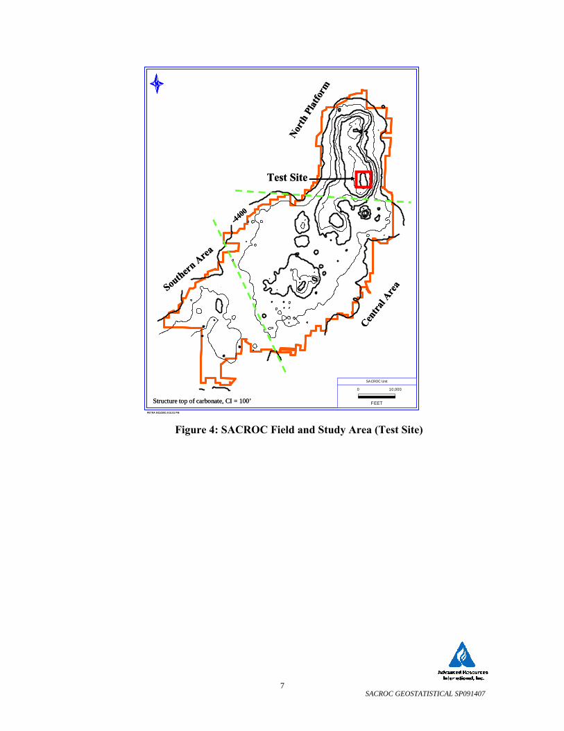
For the first stage of this project3, a study area of approximately 0.5 mi2 located in the
Northern Platform of the SACROC field was selected and is shown in Figure 4. The database consisted of 24 wells, 3 with whole core measurements of P&P through most of the section of interest, but there was no core sedimentology description, no mineralogy or petrography, and no seismic. Utilizing available well log and core data, we applied a probabilistic clustering procedure in order to:
• estimate profiles for RHOB and DT in wells that had only GR and NPHI logs; • estimate profiles for porosity and permeability in non-cored wells; • identify zones (electrofacies ~ flow units) with varying reservoir quality (RQ) based
on variations in P&P;
SACROC GEOSTATISTICAL SP091407
5
• evaluate (qualitatively) the degree to which the flow units could be correlated among wells;
• identify a vertical cyclicity that is semi-pervasive throughout the area of study and relate this cyclicity to published information concerning the seismic sequence stratigraphy of the area.
Clustering analyses indicated that the carbonate section can be divided into a suite of
closely-related flow units that have a "good" RQ (average porosity ~ 11-13 %) and into a suite of closely-related flow units that have a "poor" RQ (average porosity generally < 5 %). As interpreted from clustering analysis output, the contacts between these good and poor suites was generally rather sharp, as opposed to the generally gradational contacts that exist among the several flow units that comprise the good and poor suites. The relatively "sharp" contacts were interpreted to represent 3rd to 4th order sequence boundaries and they would likely act as significant barriers to vertical fluid flow3. We considered that this fact has important implications for enhanced recovery performance.
This two-step “soft-computing” procedure provided core-scale estimates of P&P and rock
type at well locations. In consequence, and with the aim of reservoir characterization for the study area in the SACROC Unit Platform to serve as a field demonstration, the data-driven procedure was utilized to populate the selected study area with pseudo core-scale profiles of porosity, permeability and rock types. This allowed the conditions for the application of geostatistical methods to characterize reservoirs to be improved. Legitimate models of the porosity and permeability distributions in the study area provided the basis of the second stage of this project. These models are designed to reveal the lithofacies distributions and depositional environments, providing genuine representations of permeability and porosity in concordance with the selected grid resolution for characterizing the study area.
This process provided a data set of twenty two (22) wells in the study area with foot-by-
foot profiles of P&P, and was considered to be sufficient information to characterize directly the reservoir distributions of P&P. Next, stochastic simulation algorithms were utilized to provide reservoir models of P&P in the selected study region with different levels of vertical resolution. This ability to generate reservoir parameter characterizations with a convenient vertical resolution is a beneficial tool for the efficient characterization of this complex reservoir.
With the incorporation of geostatistical tools into the characterization methodology, the
entire workflow turned evolved in to an integrated Clustering/Geostatistical approach for 3D Reservoir Characterization, which was successfully tested in the Pennsylvanian-Permian reef carbonates (Cisco and Canyon Formations) of the study area of the SACROC Unit, Horseshoe Atoll, Permian basin, Texas.
This report is focused on the application of geostatistical methods for the reservoir
characterization at SACROC. We present results derived from variogram analyses applied to P&P (actual and pseudo data), and rock types at well locations. These results were utilized to model the spatial variability of the parameters P&P. Once the corresponding models of spatial continuity of P&P were established, the stochastic simulation algorithm known as Sequential
SACROC GEOSTATISTICAL SP091407
6
Gaussian Simulation (SGS) was utilized to provide the final reservoir models of porosity and permeability in the selected study area.
Figure 3: Schematic of the Two-Step “Soft-Computing” Procedure
Log-to-Log Model
Log-to-Core Model
Borehole Seismic
(X - Well, VSP)
Borehole Seismic
(X - Well, VSP)
Borehole Seismic
(X - Well, VSP)Conventional Well Logs
(full suite)-
Conventional Well LogsConventional Well LogsConventional Well LogsHigh Resolution
Reservoir Description(core parameters)
3 - D Surface Seismic3 -D Surface Seismic3 - D Surface SeismicConventional Well Logs(partial suite)
Borehole Seismic
(X - Well, VSP)
Borehole Seismic
(X - Well, VSP)
Borehole Seismic
(X - Well, VSP)Conventional Well Logs
(full suite)-
Borehole Seismic
(X - Well, VSP)
Borehole Seismic
(X - Well, VSP)
Borehole Seismic
(X - Well, VSP)Conventional Well Logs
(full suite)-
Conventional Well LogsConventional Well LogsConventional Well LogsHigh Resolution
Reservoir Description(core parameters)
Conventional Well LogsConventional Well LogsConventional Well LogsHigh Resolution
Reservoir Description(core parameters)
3 - D Surface Seismic3 -D Surface Seismic3 - D Surface SeismicConventional Well Logs(partial suite)
3 - D Surface Seismic3 -D Surface Seismic3 - D Surface SeismicConventional Well Logs(partial suite)
SACROC GEOSTATISTICAL SP091407
7
Figure 4: SACROC Field and Study Area (Test Site)
SACROC Unit
FEET
0 10,000
PET RA 9/12/2001 8:31:51 PM
-4400
North
Plat
form
Centra
l Are
aSouthern
Area
Test Site
Structure top of carbonate, CI = 100’
SACROC Unit
FEET
0 10,000
PET RA 9/12/2001 8:31:51 PM
-4400
North
Plat
form
Centra
l Are
aSouthern
Area
Test Site
Structure top of carbonate, CI = 100’
SACROC GEOSTATISTICAL SP091407
8
2.0 Geostatistical Approach
In general terms, hybrid simulation approaches that combine two or more conditional simulation techniques are used in a geostatistical study. Because it is not realistic for a single geostatistical technique to describe all scales of heterogeneity present in a reservoir, a hybrid procedure attempts to take advantage of the best features of each simulation technique4,5,6.
A geostatistical reservoir characterization based on a hybrid approach typically begins
with building the reservoir architecture where the geometry of the units is established. Next, a geological model is determined and geobodies are populated with lithofacies, and finally the petrophysical model is generated and distributions of typical reservoir parameters are assigned to each facies.
Geostatistical simulation techniques are usually categorized in two types: pixel-based and
object-based methods4,7. Pixel-based methods are largely used to characterize reservoir parameters like porosity and permeability, but they are not designed to explicitly reproduce geometric shapes as their final goal. Yet, they can also be applied to model facies with unclear or undefined shapes.
Object-based methods are suitable to describe reservoirs with certain geometric features,
provided that adequate information (qualitative and/or quantitative) describing the geometry of reservoir bodies is available4,7. This method is frequently utilized for fluvial, deltaic and deep marine depositional environments, and when a limited number of wells with conditioning data exist. In these types of environment, the shape of most facies, such as channels, mouth bars, levees, and different types of shale, can be represented by discrete objects with well known geometric shapes. However, object-based modeling is less applicable to carbonate environments because most facies in a carbonate reservoir have experienced significant post-depositional processes (dissolution, re-precipitation, dolomitization, fracturing, etc). These processes have deteriorated the geometry of their shape, thus does not allow the utilization of known geometric objects and the estimation of their dimensions.
Geostatistical simulations of lithotypes are commonly used to create geological models
describing the heterogeneities of a reservoir. However it is difficult to assess the uncertainty of hydrocarbon-in-place correlated to facies proportions because the facies proportions are uncertain. Therefore, in the study area, variogram analysis was directly applied to the available data (22 wells with P&P profiles) to determine possible patterns of spatial variability of these parameters. With the derived variogram models, the SGS algorithm conditioned to the well data was used to generate multiple reservoir distributions of P&P at interwell locations. Corresponding average scenarios of P&P were generated from these characterizations and were utilized as input in the next step of reservoir simulation performance, and where the production data had to be honored.
SACROC GEOSTATISTICAL SP091407
9
3.0 Stratigraphic Coordinate System
An important consideration in most 3D geostatistical applications is related with the coordinates system. Due to complex geological processes, the SACROC anysotropy directions vary throughout the area with the local dips. For the variogram analysis and for the simulations, the data location coordinates were transformed to stratigraphic coordinates4. This coordinate transformation is commonly utilized for folded or variable thickness geologic bodies where principles of stratigraphy can be applied; however, for the study area of SACROC, stratigraphic conformity from the top to the bottom of the interval was assumed based on the small variability of its thickness (coefficient of variation is 0.075).
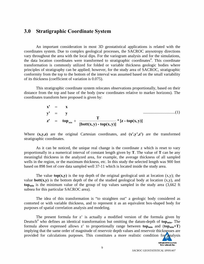
This stratigraphic coordinate system relocates observations proportionally, based on their
distance from the top and base of the body (new coordinates relative to marker horizons). The coordinates transform here proposed is given by:
y)]top(x,-[z*y)]top(x,-y)[bott(x,
T top z'
y y' x x'
min +=
==
................................(1)
Where (x,y,z) are the original Cartesian coordinates, and (x’,y’,z’) are the transformed stratigraphic coordinates.
As it can be noticed, the unique real change is the coordinate z which is reset to vary proportionally in a numerical interval of constant length given by T. The value of T can be any meaningful thickness in the analyzed area, for example, the average thickness of all sampled wells in the region, or the maximum thickness, etc. In this study the selected length was 900 feet based on 898 feet of core data sampled well 37-11 which is located inside the study area.
The value top(x,y) is the top depth of the original geological unit at location (x,y); the
value bott(x,y) is the bottom depth of the of the studied geological body at location (x,y), and topmin is the minimum value of the group of top values sampled in the study area (3,662 ft subsea for this particular SACROC area).
The idea of this transformation is “to straighten out" a geologic body considered as
contorted or with variable thickness, and to represent it as an equivalent box-shaped body for purposes of spatial correlation analysis and modeling.
The present formula for z’ is actually a modified version of the formula given by
Deutsch4 who defines an identical transformation but omitting the datum-depth of topmin. The formula above expressed allows z’ to proportionally range between topmin and (topmin+T) implying that the same order of magnitude of reservoir depth values and reservoir thicknesses are provided for calculations purposes. This constitutes a more realistic condition for analysis

SACROC GEOSTATISTICAL SP091407
10
purposes. All variogram analysis and simulations were performed in the stratigraphic system (x’,y’,z’), and the final results were back-transformed to the original Cartesian system.
SACROC GEOSTATISTICAL SP091407
11
4.0 Variogram Analysis
4.1 Methodology
Reservoir parameters are conceived as random variables varying continuously in space4,5,6,7,8. The basic geostatistical tool used to quantify the spatial variability of a reservoir parameter is the experimental semivariogram (hereafter variogram). The experimental variogram is used to identify the underlying spatial pattern and trends of reservoir variables, and reveals the randomness and the structured aspects of their spatial dispersion4,5,6,7,8. In essence, it is a plot which illustrates the way in which the dissimilarity between sample values is related to the separation distance and the direction between the sample values.
The traditional experimental semivariogram is described by the following equation4,5,6,8:
....................................(2) Where h
r is the lag, or separation vector, between two data points, )xz( i
r and )hxz( i
rr+ , h is the
module of vector hr
, and )hN(r
is the number of data pairs used in the summation (these data pairs qualify if they are separated a distance h along the direction of vector h
r). This calculation
is repeated for different values of h, and the plot of all ordered pairs (h))γ(h, ˆ provides the called experimental variogram, i.e., values of (h)γ̂ as a function of distance h (in the particular direction given by vector h
r) .
In general terms, it is expected that experimental variograms tend to level off at a “sill”
which theoretically should be equal to the empirical variance of the studied parameter data. The distance at which this stabilization occurs is referred to as the “range” of the variogram for an analyzed parameter. This range is conceived as the distance over which the sampling values cease to be spatially correlated4,5,6,8. Another important feature of experimental variograms is a discontinuity at the origin of the plot trend (non–zero intercept) known as the “nugget effect”. It is considered a random component attributable primarily to local variations occurring at scales smaller than the sampling interval.
An underlying assumption in a variogram study is that the parameter under analysis
satisfies a statistical concept known as “stationarity” which basically implies that any subset of the data has the same statistical description as any other subset4,5,6,8; in other words, they share similar characteristics such as mean and standard deviation for the property studied. This is an assumption that can be quite acceptable for data which comes from reservoirs that were subject to the same geological processes. Consequently, the sample values and predictions must be from
[ ]2)hN(
1 iii xz()hxz(
)h2N(1(h)γ ∑
=
−+=r
rrrr )ˆ
SACROC GEOSTATISTICAL SP091407
12
the same region of stationarity, in this case the reservoir, where statistical properties of the predicted phenomena are kept across space.
For geostatistical simulation purposes, similarity or spatial correlation measurements
(variogram values) are necessary for all distances and at any possible direction (within a neighborhood of the un-sampled location). However, in any study variogram values are available for specific distances and for only few directions. This fact obligates the interpolation of the variogram values for any distance h and along any possible direction, motivating the consideration of adjusting mathematical functions to the experimental variogram values capable of providing these similarity measurements for any spatial situation of the parameter.
The definitive spatial pattern of reservoir parameters for characterization purposes using
stochastic simulation algorithms is established when authorized mathematical functions are fitted to the experimental variogram obtained from the data (the mathematical condition is known as the positive definite condition)4,5,6,8. This variogram model provides the spatial correlation between parameter samples in terms of the distance and the direction between samples, and reflects the continuity and spatial variability of the studied reservoir parameter. The variogram model is the main input required by the simulation procedure SGS which produces equiprobable characterizations of reservoir parameters constrained by the data.
The more commonly used models of variogram are the exponential, spherical, Gaussian,
power models, hole effect models (cyclic), and the pure nugget effect4,5,6,8. Equations for all these models can be found in references 4, 5, 6, and 8. The spherical model can be considered as the variogram resulting from a wide variety of natural processes, and is the most popular model utilized by practitioners in tasks of stochastic reservoir characterization. This work was not an exception. Spherical models were adjusted to all analyzed experimental variograms.
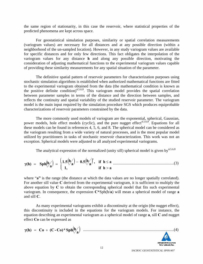
The analytical expression of the normalized (unity sill) spherical model is given by4,5,6,8
( ) ( ) ( )⎪⎩
⎪⎨⎧
>≤−==
ah if 1,ah if,a
h 0.5 ah 1.5 a
hSph γ(h)3
.............................................................(3)
where “a” is the range (the distance at which the data values are no longer spatially correlated). For another sill value C derived from the experimental variogram, it is sufficient to multiply the above equation by C to obtain the corresponding spherical model that fits such experimental variogram. In consequence, the expression C*Sph(h/a) will mean a spherical model of range a and sill C.
As many experimental variograms exhibit a discontinuity at the origin (the nugget effect), this discontinuity is included in the equations for the variogram models. For instance, the equation describing an experimental variogram as a spherical model of range a, sill C and nugget effect Co can be expressed as
( ) ahSph *Co)-(C Co γ(h) += ...........................................................................................(4)
SACROC GEOSTATISTICAL SP091407
13
where the value (Co-C) can be referred as a relative sill.
Since the positive definite condition on authorized mathematical functions holds for any linear combination of the models, a variogram model can also be a linear combination of two or more of the authorized models, each model having different values for its parameters4,5,6,8. The equations 3 and 4 are for isotropic variogram models or unidirectional. But, it is well known that within a studied reservoir, anisotropic behavior of any of its parameters, i.e. the change of the pattern of spatial variability with directionality is encountered.
Anisotropy in geostatistical analysis is often distinguished between geometric and zonal
anisotropy4,5,6,8. In geometric anisotropy, it is assumed that directional variograms have same shapes and same sill values, but different ranges are expected for different directions. In zonal anisotropy, it is understood that the sill value is a function of the direction. Mixed situations in which both sill and range values are a function of direction are also often found. This kind of anisotropy can be identified in a stratified phenomenon with a spatial variability through a layer drastically different from the variability between layers4. More details about anisotropy types associated with particular geological environments can be found in references 4 and 9.
4.2 SACROC Variography
For the variogram analysis of SACROC, actual values and pseudo values of core porosity, core permeability and rock types were utilized to calculate corresponding experimental variograms. In order to calculate the variograms of P&P and rock types, a stratigraphic or conformal transformation of vertical coordinates was carried out first to compare samples from similar stratigraphic horizons and to avoid typical differences resulting from horizontal slicing based on the original coordinate system. This kind of “unrolling” of the structure allows comparison of sample values at the same “stratigraphic horizon” when the experimental variogram is calculated. Comparisons of samples under this premise are geologically consistent because it can be expected that reservoir parameter values at the same “stratigraphic horizon” have more depositional similarities4. In consequence, resulting experimental variograms can better reveal the “hidden” spatial behavior of the variable under analysis.
Due to the size of the study area, and the significant number of wells included in the area
that have foot by foot profiles of porosity and permeability, and due to practical considerations related with the task of flow simulation (data availability, simulation objectives, grid definition, software, etc.), it was decided to characterize directly the distribution of P&P without the consideration of the rock type parameter as a possible guide. In addition, the origin of the foot-by-foot P&P pseudo values at well locations is narrowly tied to the corresponding foot-by-foot mode or rock type values at the same well locations, so this also favors a direct and less elaborate approach. Therefore, direct data of P&P was utilized for the variogram analysis and in the application of the SGS algorithm.
SACROC GEOSTATISTICAL SP091407
14
An alternative approach commonly used when facies or rock type descriptions are available at well locations is to model a spatial distribution of facies using adequate geostatistical algorithms, and later to fill these spatial “entities” with porosity, permeability, and water saturation values following the corresponding spatial behavior (variogram model) of each parameter in each rock type. Although this approach was not utilized to simplify the reservoir simulation task, indicator variogram analyses of rock types and variography studies of P&P for each rock type was performed in order to complement the global variography of P&P.
The use of Gaussian techniques (SGS algorithm) requires the fulfillment by the variable
of certain theoretical conditions. Generally, a prior transform of the available data to the congenial normal/Gaussian distribution data is performed for subsequent geostatistical analysis (variography and simulation tasks)4,5,6. This transformation automatically sets the sill value to 1 (its theoretical value). In this work, this transformation was executed by using the normal score transform4,5,6 provided by the software here utilized. This software was the Stanford Geostatistical Earth Modeling Software10 (SGEMS), and the Geostatistical Software Library5 (GSLIB) which are public domain software both provided by Stanford University.
SGEMS10 and GSLIB5 are software for 3D geostatistical modeling that implements some
classical geostatistics algorithms, as well as additional developments made at Stanford University. The geostatistical routines includes Kriging, Cokriging, Sequential Gaussian Simulation, Sequential Indicator Simulation, Multi-variate Sequential Gaussian and Indicator Simulation, Multiple-point Statistics Simulation, and other geostatistical tools for basic statistics, variography, post simulation analysis, etc. In particular, SGEMS10 was used to compute the experimental variograms of normalized porosity values, normalized permeability measurements (log10), and rock-types in both the vertical and horizontal directions. In addition, it was also utilized to fit spherical variogram models to the experimental ones, as long as there was adequate data to estimate the experimental variogram in the considered direction and for the considered variable.
In summary, the parameters describing the spatial correlation (nugget effect, sill, number
of structures, types of structures, and ranges) were obtained graphically by plotting the experimental variogram against intersample distances and then fitting corresponding theoretical models. Knowledge about the reservoir and team expertise and interpretation were used to obtain the corresponding models that matched empirical variograms.
The nugget effect value and general structure of the models were obtained from vertical
variograms and were extended to horizontal (areal) variograms. Directional horizontal variograms were constructed in eight directions under the assumption that the stratigraphic transformation of coordinates produces the effect of sample pairs belong to the same bedding plane or stratigraphic horizon. These directional variograms describe the relationship between data pairs oriented in a specified direction, and they are used to determine whether the spatially distributed data are anisotropic. If spatial correlations are independent of directionality, it is indicative that reservoir data has an isotropic spatial behavior4,5,6,7,8.
As mentioned, the range represents the maximum distance of spatial correlation, and it
can vary in different directions. The minimum and maximum ranges obtained from the
SACROC GEOSTATISTICAL SP091407
15
directional variograms should correspond to the anisotropy axes of spatial continuity (assuming that geometric anisotropy4,5,6,7,8 exists), and in planes parallel to bedding.
Anisotropy ellipses are typically constructed by plotting the range versus the direction
vector for each data set4,5,6,7,8. We used the variogram analysis option of software SGEMS10 to calculate the experimental variograms. In this software (and in GSLIB5), one, two or three-dimensional variogram analysis can be executed.
The one-dimensional (1D) analysis compares the points linearly, and needs three
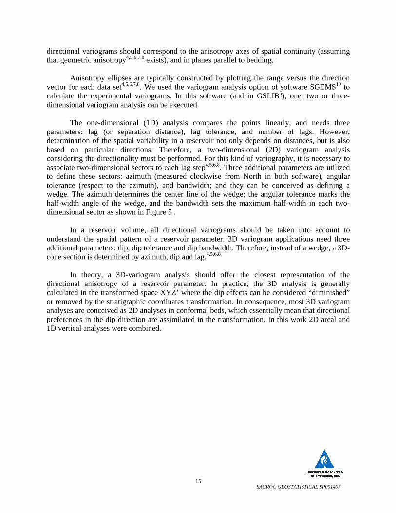
parameters: lag (or separation distance), lag tolerance, and number of lags. However, determination of the spatial variability in a reservoir not only depends on distances, but is also based on particular directions. Therefore, a two-dimensional (2D) variogram analysis considering the directionality must be performed. For this kind of variography, it is necessary to associate two-dimensional sectors to each lag step4,5,6,8. Three additional parameters are utilized to define these sectors: azimuth (measured clockwise from North in both software), angular tolerance (respect to the azimuth), and bandwidth; and they can be conceived as defining a wedge. The azimuth determines the center line of the wedge; the angular tolerance marks the half-width angle of the wedge, and the bandwidth sets the maximum half-width in each two-dimensional sector as shown in Figure 5 .
In a reservoir volume, all directional variograms should be taken into account to
understand the spatial pattern of a reservoir parameter. 3D variogram applications need three additional parameters: dip, dip tolerance and dip bandwidth. Therefore, instead of a wedge, a 3D-cone section is determined by azimuth, dip and lag.4,5,6,8
In theory, a 3D-variogram analysis should offer the closest representation of the
directional anisotropy of a reservoir parameter. In practice, the 3D analysis is generally calculated in the transformed space XYZ’ where the dip effects can be considered “diminished” or removed by the stratigraphic coordinates transformation. In consequence, most 3D variogram analyses are conceived as 2D analyses in conformal beds, which essentially mean that directional preferences in the dip direction are assimilated in the transformation. In this work 2D areal and 1D vertical analyses were combined.
SACROC GEOSTATISTICAL SP091407
16
Figure 5: Directional “Wedge” and Utilized Parameters for 2D Variogram Analysis.
4.3 Porosity Variography
Modeling the spatial relationship of a reservoir attribute is one of the most important tasks in constructing reservoir characterization using geostatistical methodology. Multiple scales of heterogeneity can generally be found to a degree in all depositional settings. In the reef-carbonate depositional environment of SACROC, different scales of variability can be seen in variograms of porosity, and these different scales of variability are modeled using nested variograms (linear combinations).
Porosity values at well locations (actual measurements and pseudo data) were initially
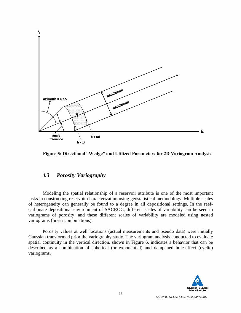
Gaussian transformed prior the variography study. The variogram analysis conducted to evaluate spatial continuity in the vertical direction, shown in Figure 6, indicates a behavior that can be described as a combination of spherical (or exponential) and dampened hole-effect (cyclic) variograms.
bandwidth
bandwidth
angletolerance
h - tol
h + tol
h
N
E
azimuth = 67.5°bandwidth
bandwidth
angletolerance
h - tol
h + tol
h
N
E
azimuth = 67.5°
SACROC GEOSTATISTICAL SP091407
17
Figure 6: Vertical Experimental Variogram of Normalized Porosity
A hole-effect variogram is associated to geologic cyclicity. Because geological processes can repeat over geologic time leading to cyclic repetition of facies and petrophysical properties, cyclic behavior can appear in experimental variograms4,7. The experimental variogram can alternate from positive correlations to negative correlations at a length scale directly linked to the geologic cycles. In SACROC, the cyclicity effect in the vertical direction can be associated with the carbonate buildups. Relative sea level “rise and fall” occurred quickly and repeatedly, providing a variety of depositional environments and facies repeating in geological time.
However, this dampened hole-effect structure only applies in the vertical direction as
seen in Figure 7 where other experimental variograms of the normalized porosity representing horizontal variability in several directions are simultaneously shown. Due to this and because both types of empirical variograms, vertical and horizontal, reach the unity sill, the experimental variogram in the vertical direction was modeled as a combination of a nugget effect component and two nested structures conceived as spherical models of spatial variability (hole effect variogram model was not considered). Figure 6 also shows the nested variogram model (solid line) fit to the vertical experimental variogram of normalized porosity. The analytical expression of this model is given by4,5,6,8
( ) ( ) 230
hSph *0.35 20hSph *0.55 0.1 γ(h) ++= ................................................................(5)
The vertical variogram model, shown in Figure 6 superimposed on to the experimental
variogram, illustrates the correlation structures of the data, and indicates that depositional environments and facies are primarily correlated at a shorter separation distance of 20 feet and more globally correlated at a larger correlation scale of 230 feet. This first range of 20 feet is the half of an apparent period of 40 feet (geological cycles are not perfectly constant) shown on the dampened cyclic variations of the experimental variogram trajectory as separation distances

SACROC GEOSTATISTICAL SP091407
18
increase. This behavior can also be observed on experimental variograms of different rock types, and particularly coincided with the range found for rock types 2 and 3 (see section 4.6) when the vertical variography of rock types was developed for a more simplified classification of only four groups of rock (instead of the original classification of ten types).
Figure 7: Directional Experimental Variograms of Normalized Porosity
Figure 7 depicts eight superimposed experimental variograms of normalized porosity in the directions 0°, 30°, 45°, 60°, 90°, 120°, 135°, and 150°, and where angles are measured clockwise from the axis North-South (0°). These horizontal variograms exhibit high nugget values, but they are not used in the model variogram because a high nugget value in the variogram model can cause the simulated parameter to be noisy or irregular which is a behavior that does not reflect reality. For these experimental horizontal variograms, it is difficult to define a variogram value at short lag distances due to the lack of parameter samples between 0 and 400 feet, and possibly other data anomalies4,5,6,8. In consequence, the nugget effect value is derived from the vertical variography since, in theory, the horizontal and vertical variograms should share the same nugget value4,5,6,8. So it is common practice to consider the vertical variogram for the nugget estimation purposes, since vertical variograms are generally calculated from abundant sampled data and can reflect short-scale variability more accurately.
As it can be seen, these experimental variograms showed very similar behaviors at the
first four lag steps (basic lag unit is 400 feet) which made elucidating the horizontal anisotropy of porosity difficult. We believe that geological characteristics of SACROC, the “smoothed” feature of possible extreme values of the pseudo porosity data, and the relatively small size of the study area (only permitting a limited manifestation of the horizontal spatial variability), explain the similarity of the spatial pattern of these directional variograms. The smoothed character of extreme porosity values is due to their origin (values obtained by using probabilistic clustering methods based on Gaussian models), and the normalization condition requested for any parameter prior the application of the SGS algorithm.

SACROC GEOSTATISTICAL SP091407
19
However, based on the nested structures modeled for the vertical variogram, the analysis
and modeling (individual and jointly) of all directional variograms, and geological knowledge of the reservoir, a model of geometric anisotropy was adopted to describe the horizontal spatial variability of (normalized) porosity for this study area. The horizontal model is represented by an isotropic nugget structure and two structures with geometric anisotropy reflecting an intermediate and a global scale. Variance values (sill, relative sill values, and nugget effect) of horizontal models honor those values derived from the vertical variography.
The geometric anisotropy of a petroleum reservoir can be conceived in terms of ellipses
(or ellipsoids) established by a single angle identifying the “major” and “minor” horizontal directions of continuity. For an ellipsoid, the vertical direction is perpendicular to the plane constituted by the two horizontal directions of continuity. Dip effects have been assimilated in the transformation of original coordinates to stratigraphic coordinates, so 3D variogram analyses are conceived as 2D analyses in conformal beds for practical purposes. The lengths of both ellipses semi-axis are identified with the ranges on the major and minor directions of continuity.
The final model for the horizontal variability of porosity variograms is summarized in
Table 1.
Table 1: Parameter Values for Horizontal Geometric Anisotropy of Normalized Porosity Geometric Anisotropy
Main Direction
Major Range (ft.)
Minor Range (ft)
Anisotropy Coefficient Scale
Structure 1 N45°E 480 460 0.96 Intermediate Structure 2 N0°E 1880 1070 0.57 Global
This model can be conceived as two superimposed ellipses. One ellipse representing the
global pattern of spatial variability with main axis aligned to the North-South direction and major and minor ranges of 1880 feet and 1070 feet respectively. The major scale reflects spatial variability aligned in the direction of the main structural trend of the reservoir and is named Structure 2 in Table 1. This greater variogram range along the direction of the structural axis can be explained by the characteristics of the SACROC limestone reef. Aside from pinnacle development in some areas at low sea-level stands, the reef generally had a low mound shape with gently dipping flanks. It is about 25 miles long (north-south) and from 4 to 7 miles wide (east-west), located along the eastern flank of the giant Horseshoe Atoll.
The intermediate scale of spatial variability is represented by a second ellipse with minor
and major ranges of 460 ft and 480 ft respectively (Structure 1 in Table 1), and is aligned to the direction N45°E as seen in Figure 8. In general terms, most directional variograms could be modeled with an identical first range (first structure) around 470 feet. This first structure reflecting the intermediate scale of variability tends to be more isotropic and it can be associated to complex patterns of depositional setting of sediments that provided later opportunities for erosion and diagenesis. The equation representing the variogram model4,5,6,8 at the direction of major continuity N0°E of the second or global structure is given by

SACROC GEOSTATISTICAL SP091407
20
( ) ( ) 1880hSph *0.35 470
hSph *0.55 0.1 γ(h) ++= ............................................................(6)
Figure 8: Superimposed Anisotropy Ellipses Describing the Nested Scales of the
Porosity Spatial Variability
Experimental variogram and its respective fit model can be seen in Figure 9.
Figure 9: Experimental and Model Variograms of Normalized Porosity at N0°E
Likewise, the analytical expression of the variogram model4,5,6,8 at the direction of major
continuity N45°E of the first or intermediate structure is given by
( ) ( ) 1530hSph *0.35 480
hSph *0.55 0.1 γ(h) ++= ............................................................(7)
E
N
45°
E
N
45°
SACROC GEOSTATISTICAL SP091407
21
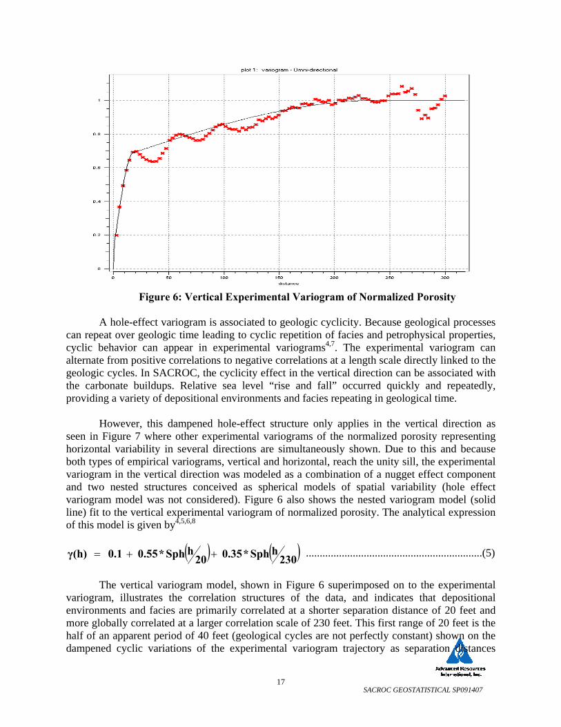
Experimental variogram and its corresponding fit model can be seen in Figure 10.
Figure 10: Experimental and Model Variograms of Normalized Porosity at N45°E
4.4 Permeability Variography
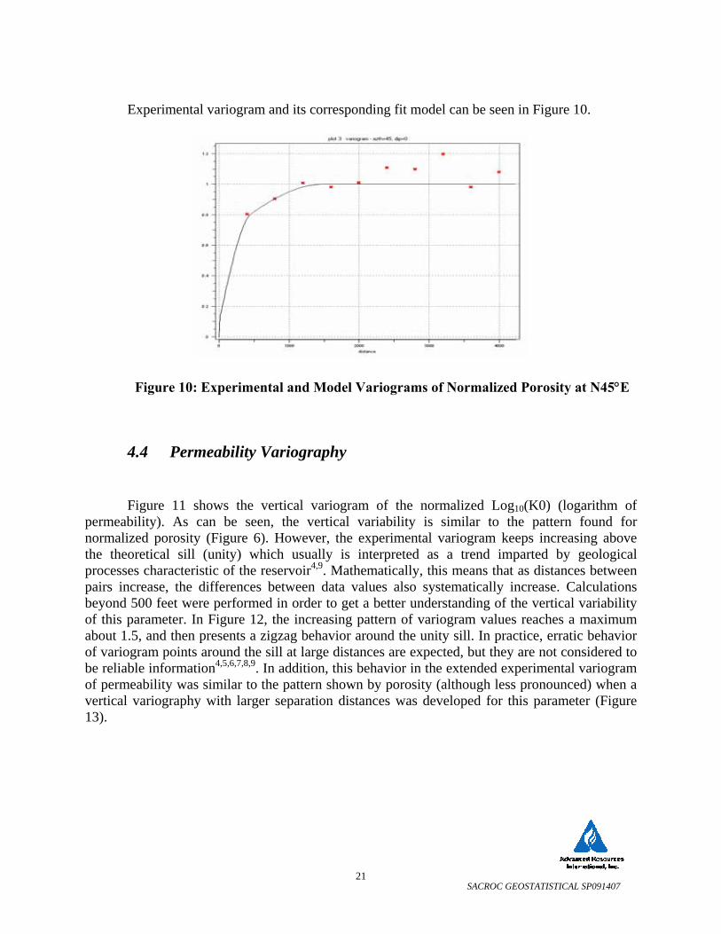
Figure 11 shows the vertical variogram of the normalized Log10(K0) (logarithm of permeability). As can be seen, the vertical variability is similar to the pattern found for normalized porosity (Figure 6). However, the experimental variogram keeps increasing above the theoretical sill (unity) which usually is interpreted as a trend imparted by geological processes characteristic of the reservoir4,9. Mathematically, this means that as distances between pairs increase, the differences between data values also systematically increase. Calculations beyond 500 feet were performed in order to get a better understanding of the vertical variability of this parameter. In Figure 12, the increasing pattern of variogram values reaches a maximum about 1.5, and then presents a zigzag behavior around the unity sill. In practice, erratic behavior of variogram points around the sill at large distances are expected, but they are not considered to be reliable information4,5,6,7,8,9. In addition, this behavior in the extended experimental variogram of permeability was similar to the pattern shown by porosity (although less pronounced) when a vertical variography with larger separation distances was developed for this parameter (Figure 13).

SACROC GEOSTATISTICAL SP091407
22
Figure 11: Experimental Vertical Variogram of Normalized Log10(K0)
Figure 12: Extended Vertical Variogram of Normalized Log10(K0)
SACROC GEOSTATISTICAL SP091407
23
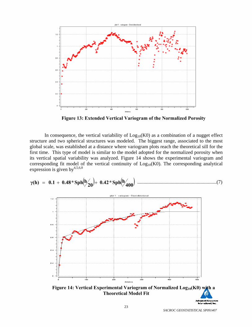
Figure 13: Extended Vertical Variogram of the Normalized Porosity
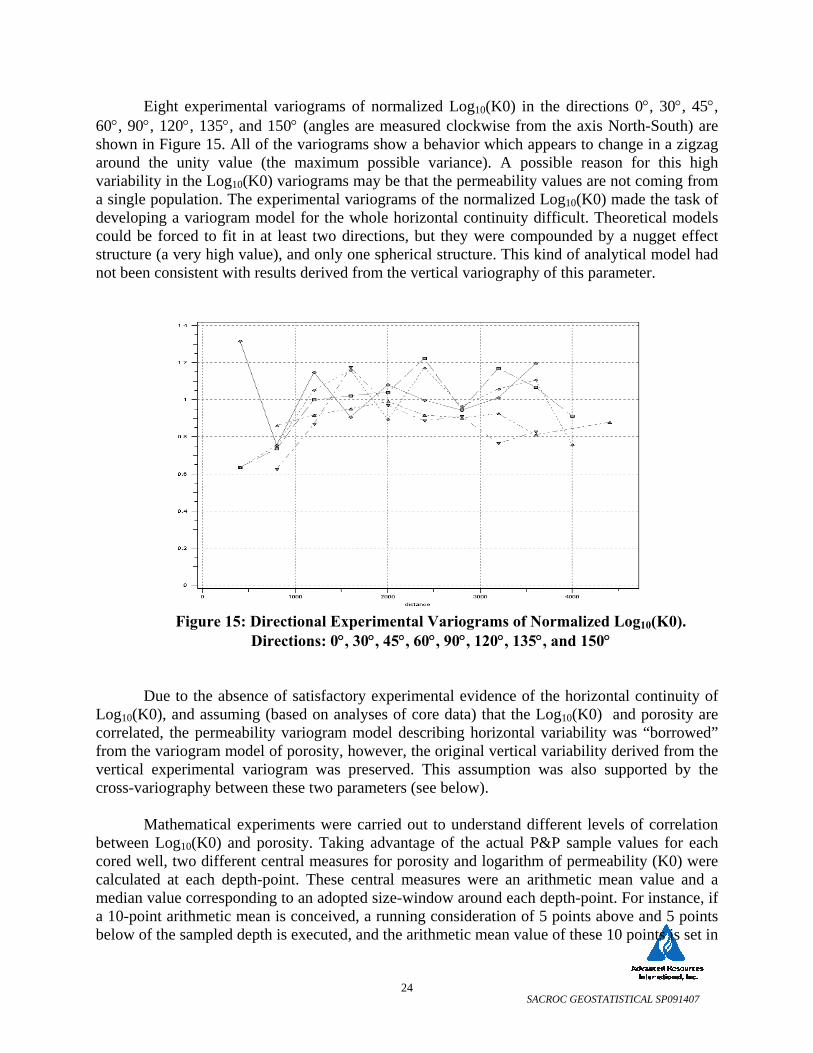
In consequence, the vertical variability of Log10(K0) as a combination of a nugget effect
structure and two spherical structures was modeled. The biggest range, associated to the most global scale, was established at a distance where variogram plots reach the theoretical sill for the first time. This type of model is similar to the model adopted for the normalized porosity when its vertical spatial variability was analyzed. Figure 14 shows the experimental variogram and corresponding fit model of the vertical continuity of Log10(K0). The corresponding analytical expression is given by4,5,6,8
( ) ( ) 400hSph *0.42 20
hSph *0.48 0.1 γ(h) ++= ................................................................(7)
Figure 14: Vertical Experimental Variogram of Normalized Log10(K0) with a Theoretical Model Fit
SACROC GEOSTATISTICAL SP091407
24
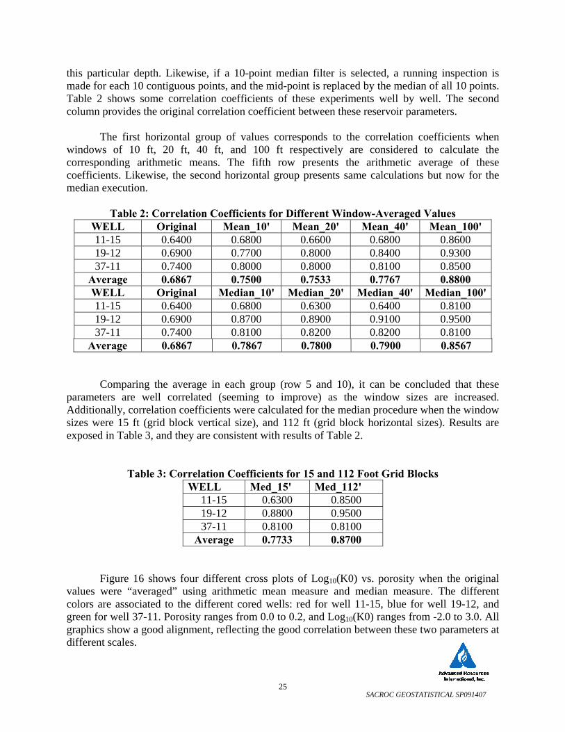
Eight experimental variograms of normalized Log10(K0) in the directions 0°, 30°, 45°, 60°, 90°, 120°, 135°, and 150° (angles are measured clockwise from the axis North-South) are shown in Figure 15. All of the variograms show a behavior which appears to change in a zigzag around the unity value (the maximum possible variance). A possible reason for this high variability in the Log10(K0) variograms may be that the permeability values are not coming from a single population. The experimental variograms of the normalized Log10(K0) made the task of developing a variogram model for the whole horizontal continuity difficult. Theoretical models could be forced to fit in at least two directions, but they were compounded by a nugget effect structure (a very high value), and only one spherical structure. This kind of analytical model had not been consistent with results derived from the vertical variography of this parameter.
Figure 15: Directional Experimental Variograms of Normalized Log10(K0). Directions: 0°, 30°, 45°, 60°, 90°, 120°, 135°, and 150°
Due to the absence of satisfactory experimental evidence of the horizontal continuity of
Log10(K0), and assuming (based on analyses of core data) that the Log10(K0) and porosity are correlated, the permeability variogram model describing horizontal variability was “borrowed” from the variogram model of porosity, however, the original vertical variability derived from the vertical experimental variogram was preserved. This assumption was also supported by the cross-variography between these two parameters (see below).
Mathematical experiments were carried out to understand different levels of correlation
between Log10(K0) and porosity. Taking advantage of the actual P&P sample values for each cored well, two different central measures for porosity and logarithm of permeability (K0) were calculated at each depth-point. These central measures were an arithmetic mean value and a median value corresponding to an adopted size-window around each depth-point. For instance, if a 10-point arithmetic mean is conceived, a running consideration of 5 points above and 5 points below of the sampled depth is executed, and the arithmetic mean value of these 10 points is set in
SACROC GEOSTATISTICAL SP091407
25
this particular depth. Likewise, if a 10-point median filter is selected, a running inspection is made for each 10 contiguous points, and the mid-point is replaced by the median of all 10 points. Table 2 shows some correlation coefficients of these experiments well by well. The second column provides the original correlation coefficient between these reservoir parameters.
The first horizontal group of values corresponds to the correlation coefficients when
windows of 10 ft, 20 ft, 40 ft, and 100 ft respectively are considered to calculate the corresponding arithmetic means. The fifth row presents the arithmetic average of these coefficients. Likewise, the second horizontal group presents same calculations but now for the median execution.
Table 2: Correlation Coefficients for Different Window-Averaged Values
WELL Original Mean_10' Mean_20' Mean_40' Mean_100' 11-15 0.6400 0.6800 0.6600 0.6800 0.8600 19-12 0.6900 0.7700 0.8000 0.8400 0.9300 37-11 0.7400 0.8000 0.8000 0.8100 0.8500
Average 0.6867 0.7500 0.7533 0.7767 0.8800 WELL Original Median_10' Median_20' Median_40' Median_100'11-15 0.6400 0.6800 0.6300 0.6400 0.8100 19-12 0.6900 0.8700 0.8900 0.9100 0.9500 37-11 0.7400 0.8100 0.8200 0.8200 0.8100
Average 0.6867 0.7867 0.7800 0.7900 0.8567
Comparing the average in each group (row 5 and 10), it can be concluded that these parameters are well correlated (seeming to improve) as the window sizes are increased. Additionally, correlation coefficients were calculated for the median procedure when the window sizes were 15 ft (grid block vertical size), and 112 ft (grid block horizontal sizes). Results are exposed in Table 3, and they are consistent with results of Table 2.
Table 3: Correlation Coefficients for 15 and 112 Foot Grid Blocks WELL Med_15' Med_112'
11-15 0.6300 0.8500 19-12 0.8800 0.9500 37-11 0.8100 0.8100
Average 0.7733 0.8700
Figure 16 shows four different cross plots of Log10(K0) vs. porosity when the original values were “averaged” using arithmetic mean measure and median measure. The different colors are associated to the different cored wells: red for well 11-15, blue for well 19-12, and green for well 37-11. Porosity ranges from 0.0 to 0.2, and Log10(K0) ranges from -2.0 to 3.0. All graphics show a good alignment, reflecting the good correlation between these two parameters at different scales.

SACROC GEOSTATISTICAL SP091407
26
Returning to the variogram analysis, when both vertical models (porosity and permeability) are compared, both models present a first range of 20 feet (intermediate scale) although different global scale ranges. The identification between the first ranges permits the use directly of the same geometric anisotropy of porosity for the first structure of permeability. For the second global scale, the ratio between corresponding global ranges (permeability-range/porosity-range) was calculated to utilize this proportionality in determining ranges for the horizontal variability of permeability data relative to the equivalent porosity data. This factor is approximately 1.74, and resultant variogram models for permeability were assumed similar to the porosity variogram models, but with global scale range augmented by a factor of 1.74. The same anisotropy ellipses of directionality were assumed. For the horizontal variogram models of normalized permeability, variance values are equal to those derived from the vertical variography.
Figure 16: Window Averaged Permeability (Logarithm) and Porosity
The final model for the horizontal variability of permeability variograms is summarized
on Table 4.
0 0.05 0.1 0.15 0.2
-2
-1
0
1
2
Median 100’porosity
Log 1
0(K
0)
0 0.05 0.1 0.15 0.2
-2
-1
0
1
2
3
Average 10’
porosity
porosity
Log 1
0(K
0)
0 0.05 0.1 0.15 0.2
-2
-1
0
1
2
Average 100’porosity
Log 1
0(K
0)
0 0.05 0.1 0.15 0.2
-2
-1
0
1
2
3
Median 10’
Log 1
0(K
0)
0 0.05 0.1 0.15 0.2
-2
-1
0
1
2
Median 100’porosity
Log 1
0(K
0)
0 0.05 0.1 0.15 0.2
-2
-1
0
1
2
Median 100’0 0.05 0.1 0.15 0.2
-2
-1
0
1
2
Median 100’porosity
Log 1
0(K
0)
0 0.05 0.1 0.15 0.2
-2
-1
0
1
2
3
Average 10’
porosity
porosity
Log 1
0(K
0)
0 0.05 0.1 0.15 0.2
-2
-1
0
1
2
Average 100’porosity
Log 1
0(K
0)
0 0.05 0.1 0.15 0.2
-2
-1
0
1
2
3
Median 10’
Log 1
0(K
0)
0 0.05 0.1 0.15 0.2
-2
-1
0
1
2
3
Average 10’
porosity
porosity
Log 1
0(K
0)
0 0.05 0.1 0.15 0.2
-2
-1
0
1
2
3
Average 10’0 0.05 0.1 0.15 0.2
-2
-1
0
1
2
3
Average 10’
porosity
porosity
Log 1
0(K
0)
0 0.05 0.1 0.15 0.2
-2
-1
0
1
2
Average 100’porosity
Log 1
0(K
0)
0 0.05 0.1 0.15 0.2
-2
-1
0
1
2
Average 100’0 0.05 0.1 0.15 0.2
-2
-1
0
1
2
Average 100’porosity
Log 1
0(K
0)
0 0.05 0.1 0.15 0.2
-2
-1
0
1
2
3
Median 10’
Log 1
0(K
0)
0 0.05 0.1 0.15 0.2
-2
-1
0
1
2
3
Median 10’0 0.05 0.1 0.15 0.2
-2
-1
0
1
2
3
Median 10’
Log 1
0(K
0)
SACROC GEOSTATISTICAL SP091407
27
Table 4: Summary of Parameter Values Describing the Horizontal Geometric Anisotropy of Normalized Permeability
Geometric Anisotropy
Main Direction
Major Range (ft.)
Minor Range (ft)
Anisotropy Coefficient Scale
Structure 1 N45°E 480 460 0.96 Intermediate Structure 2 N0°E 3270 1860 0.57 Global
4.5 Cross-Variogram Analysis
Application of Gaussian algorithms to simulate a primary variable guided by a secondary correlated variable can require a model of the crossed spatial variability between both parameters. As mentioned previously, we assumed that the logarithm of permeability is correlated to porosity, and this fact is also used to characterize the distribution of permeability in the study area of SACROC. In consequence, a cross variography study was developed between normalized porosity and normalized logarithm of permeability in order to determine possible patterns of crossed continuity between these parameters.
Figures 17 and 18 illustrate the vertical cross variability between normalized porosity and
normalized permeability (Log10). Figure 17 presents the experimental variogram, and shows a very similar variability to the patterns previously found for normalized Log10(K0) and for normalized porosity (Figures 12 and 13 respectively). Again, this experimental variogram increased above the theoretical sill (unity) ratifying the similar trend found in the vertical variography of these parameters when they were analyzed individually. Following previous variogram models as guidelines, the crossed vertical variability between porosity and Log10(K0) was modeled as a combination of a nugget effect structure and two spherical structures. The global scale range (corresponding to the second structure) was fixed at the distance where variogram plots reached the theoretical sill for the first time. Figure 17 shows the experimental crossed variogram (vertical) with the corresponding model of continuity fit to the data. The analytical expression is given by4,5,6,8
( ) ( ) 375hSph *0.425 20
hSph *0.475 0.1 γ(h) ++= ............................................................(8)
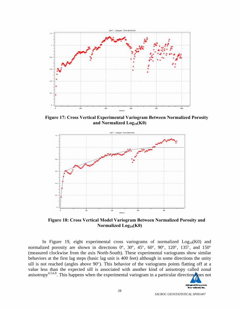
SACROC GEOSTATISTICAL SP091407
28
Figure 17: Cross Vertical Experimental Variogram Between Normalized Porosity and Normalized Log10(K0)
Figure 18: Cross Vertical Model Variogram Between Normalized Porosity and Normalized Log10(K0)
In Figure 19, eight experimental cross variograms of normalized Log10(K0) and normalized porosity are shown in directions 0°, 30°, 45°, 60°, 90°, 120°, 135°, and 150° (measured clockwise from the axis North-South). These experimental variograms show similar behaviors at the first lag steps (basic lag unit is 400 feet) although in some directions the unity sill is not reached (angles above 90°). This behavior of the variograms points flatting off at a value less than the expected sill is associated with another kind of anisotropy called zonal anisotropy4,5,6,8. This happens when the experimental variogram in a particular direction does not
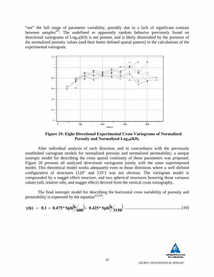
SACROC GEOSTATISTICAL SP091407
29
“see” the full range of parameter variability, possibly due to a lack of significant contrast between samples4,9. The undefined or apparently random behavior previously found on directional variograms of Log10(K0) is not present, and is likely diminished by the presence of the normalized porosity values (and their better defined spatial pattern) in the calculations of the experimental variogram.
Figure 19: Eight Directional Experimental Cross Variograms of Normalized Porosity and Normalized Log10(K0).
After individual analysis of each direction, and in concordance with the previously
established variogram models for normalized porosity and normalized permeability, a unique isotropic model for describing the cross spatial continuity of these parameters was proposed. Figure 20 presents all analyzed directional variograms jointly with the same superimposed model. This theoretical model works adequately even in those directions where a well defined configuration of structures (120° and 135°) was not obvious. The variogram model is compounded by a nugget effect structure, and two spherical structures honoring those variance values (sill, relative sills, and nugget effect) derived from the vertical cross variography.
The final isotropic model for describing the horizontal cross variability of porosity and
permeability is expressed by the equation4,5,6,8.
( ) ( ) 3150hSph *0.425 600
hSph *0.475 0.1 γ(h) ++= ......................................................(10)
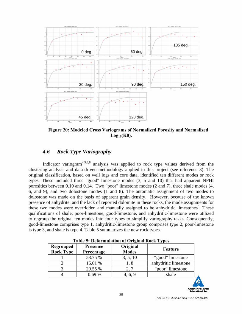
SACROC GEOSTATISTICAL SP091407
30
Figure 20: Modeled Cross Variograms of Normalized Porosity and Normalized Log10(K0).
4.6 Rock Type Variography
Indicator variogram4,5,6,8 analysis was applied to rock type values derived from the clustering analysis and data-driven methodology applied in this project (see reference 3). The original classification, based on well logs and core data, identified ten different modes or rock types. These included three "good" limestone modes (3, 5 and 10) that had apparent NPHI porosities between 0.10 and 0.14. Two "poor" limestone modes (2 and 7), three shale modes (4, 6, and 9), and two dolostone modes (1 and 8). The automatic assignment of two modes to dolostone was made on the basis of apparent grain density. However, because of the known presence of anhydrite, and the lack of reported dolomite in these rocks, the mode assignments for these two modes were overridden and manually assigned to be anhydritic limestones3. These qualifications of shale, poor-limestone, good-limestone, and anhydritic-limestone were utilized to regroup the original ten modes into four types to simplify variography tasks. Consequently, good-limestone comprises type 1, anhydritic-limestone group comprises type 2, poor-limestone is type 3, and shale is type 4. Table 5 summarizes the new rock types.
Table 5: Reformulation of Original Rock Types Regrouped Rock Type
Presence Percentage
Original Modes Feature
1 53.75 % 3, 5, 10 “good” limestone 2 16.01 % 1, 8 anhydritic limestone 3 29.55 % 2, 7 “poor” limestone 4 0.69 % 4, 6, 9 shale
0 deg.
30 deg.
45 deg.
60 deg.
90 deg.
120 deg.
135 deg.
150 deg.
0 deg.
30 deg.
45 deg.
60 deg.
90 deg.
120 deg.
135 deg.
150 deg.
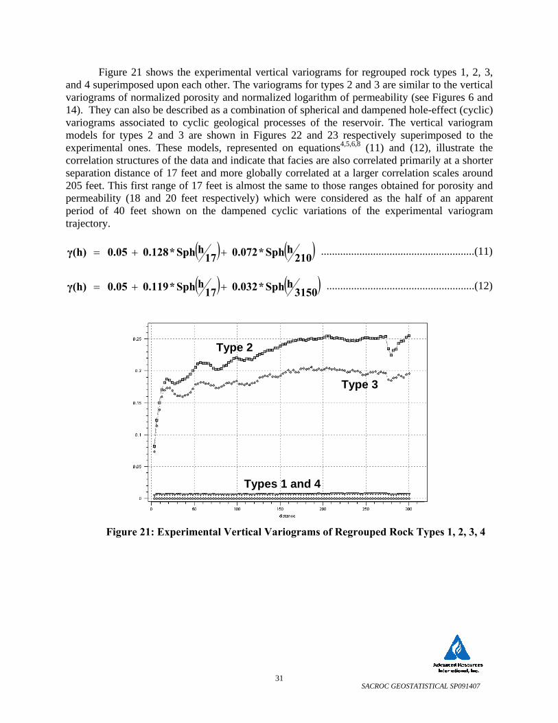
SACROC GEOSTATISTICAL SP091407
31
Figure 21 shows the experimental vertical variograms for regrouped rock types 1, 2, 3, and 4 superimposed upon each other. The variograms for types 2 and 3 are similar to the vertical variograms of normalized porosity and normalized logarithm of permeability (see Figures 6 and 14). They can also be described as a combination of spherical and dampened hole-effect (cyclic) variograms associated to cyclic geological processes of the reservoir. The vertical variogram models for types 2 and 3 are shown in Figures 22 and 23 respectively superimposed to the experimental ones. These models, represented on equations4,5,6,8 (11) and (12), illustrate the correlation structures of the data and indicate that facies are also correlated primarily at a shorter separation distance of 17 feet and more globally correlated at a larger correlation scales around 205 feet. This first range of 17 feet is almost the same to those ranges obtained for porosity and permeability (18 and 20 feet respectively) which were considered as the half of an apparent period of 40 feet shown on the dampened cyclic variations of the experimental variogram trajectory.
( ) ( ) 210
hSph *0.072 17hSph *0.128 0.05 γ(h) ++= ........................................................(11)
( ) ( ) 3150
hSph *0.032 17hSph *0.119 0.05 γ(h) ++= ......................................................(12)
Figure 21: Experimental Vertical Variograms of Regrouped Rock Types 1, 2, 3, 4
Type 2
Type 3
Types 1 and 4
Type 2
Type 3
Types 1 and 4
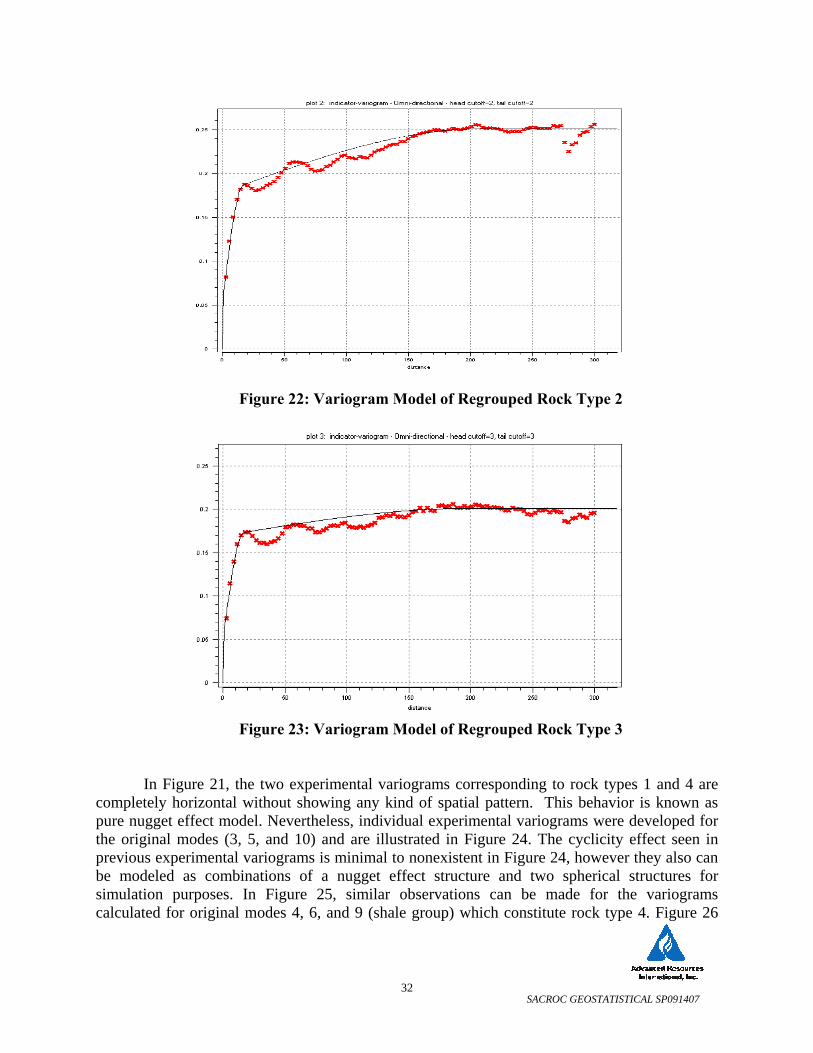
SACROC GEOSTATISTICAL SP091407
32
Figure 22: Variogram Model of Regrouped Rock Type 2
Figure 23: Variogram Model of Regrouped Rock Type 3
In Figure 21, the two experimental variograms corresponding to rock types 1 and 4 are
completely horizontal without showing any kind of spatial pattern. This behavior is known as pure nugget effect model. Nevertheless, individual experimental variograms were developed for the original modes (3, 5, and 10) and are illustrated in Figure 24. The cyclicity effect seen in previous experimental variograms is minimal to nonexistent in Figure 24, however they also can be modeled as combinations of a nugget effect structure and two spherical structures for simulation purposes. In Figure 25, similar observations can be made for the variograms calculated for original modes 4, 6, and 9 (shale group) which constitute rock type 4. Figure 26
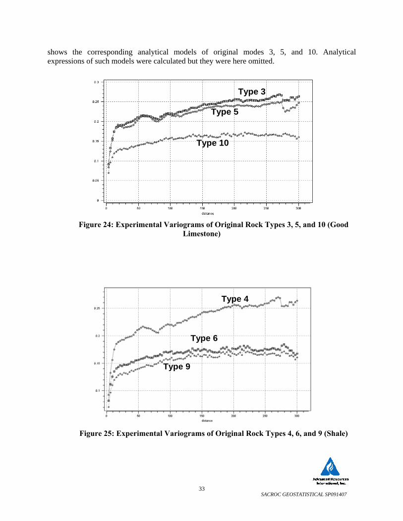
SACROC GEOSTATISTICAL SP091407
33
shows the corresponding analytical models of original modes 3, 5, and 10. Analytical expressions of such models were calculated but they were here omitted.
Figure 24: Experimental Variograms of Original Rock Types 3, 5, and 10 (Good
Limestone)
Figure 25: Experimental Variograms of Original Rock Types 4, 6, and 9 (Shale)
Type 3
Type 10
Type 5
Type 3
Type 10
Type 5
Type 4
Type 9
Type 6
Type 4
Type 9
Type 6

SACROC GEOSTATISTICAL SP091407
34
Figure 26: Variogram Models Fit to Experimental Variograms of Original Modes 3, 5, and 10 (Good Limestone)
Figure 27 depicts horizontal experimental variograms of all regrouped rock types at
directions 0°, 45°, 90°, and 135° (clockwise measured from North-South axis). Three groups of plots are clearly visible. The first group of plots correspond to rock types 1 and 4, and similar to the vertical case, show very little structure at each direction. The second group of plots has the highest variance values, and is associated exclusively to rock type 2. These variograms are very similar in each direction and could be modeled utilizing a unique isotropic model in concordance with the variance values, number, and kind of structures derived from the corresponding vertical variography. Below, the horizontal isotropic model4,5,6,8 proposed for type 2:
( ) ( ) 1680hSph *0.072 385
hSph *0.128 0.05 γ(h) ++= ...................................................(13)
The third recognizable group of plots of intermediate variance values are associated with
rock type 3. These also present similarities which would allow using a unique isotropic model guided by results of the corresponding vertical variography for this rock type. The analytical expression is given by4,5,6,8
( ) ( ) 1830hSph *0.072 860
hSph *0.119 0.05 γ(h) ++= ....................................................(14)
Type 10
Type 3 Type 5
Type 10Type 10
Type 3 Type 5Type 3Type 3 Type 5Type 5
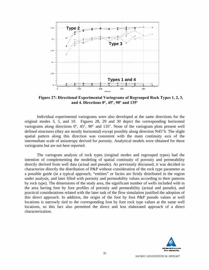
SACROC GEOSTATISTICAL SP091407
35
Figure 27: Directional Experimental Variograms of Regrouped Rock Types 1, 2, 3, and 4. Directions 0°, 45°, 90° and 135°
Individual experimental variograms were also developed at the same directions for the original modes 3, 5, and 10. Figures 28, 29 and 30 depict the corresponding horizontal variograms along directions 0°, 45°, 90° and 135°. None of the variogram plots present well defined structures (they are mostly horizontal) except possibly along direction N45°S. The slight spatial pattern along this direction was consistent with the main continuity axis of the intermediate scale of anisotropy derived for porosity. Analytical models were obtained for these variograms but are not here reported.
The variogram analysis of rock types (original modes and regrouped types) had the
intention of complementing the modeling of spatial continuity of porosity and permeability directly derived from well data (actual and pseudo). As previously discussed, it was decided to characterize directly the distribution of P&P without consideration of the rock type parameter as a possible guide (in a typical approach, “entities” or facies are firstly distributed in the region under analysis, and later filled with porosity and permeability values according to their patterns by rock type). The dimensions of the study area, the significant number of wells included with in the area having foot by foot profiles of porosity and permeability (actual and pseudo), and practical considerations related with the later task of the flow simulation justified the adoption of this direct approach. In addition, the origin of the foot by foot P&P pseudo values at well locations is narrowly tied to the corresponding foot by foot rock type values at the same well locations, so this fact also permitted the direct and less elaborated approach of a direct characterization.
Types 1 and 4
Type 2
Type 3
Types 1 and 4
Type 2
Type 3
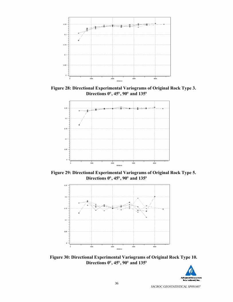
SACROC GEOSTATISTICAL SP091407
36
Figure 28: Directional Experimental Variograms of Original Rock Type 3.
Directions 0°, 45°, 90° and 135°
Figure 29: Directional Experimental Variograms of Original Rock Type 5.
Directions 0°, 45°, 90° and 135° Figure 30: Directional Experimental Variograms of Original Rock Type 10.
Directions 0°, 45°, 90° and 135°
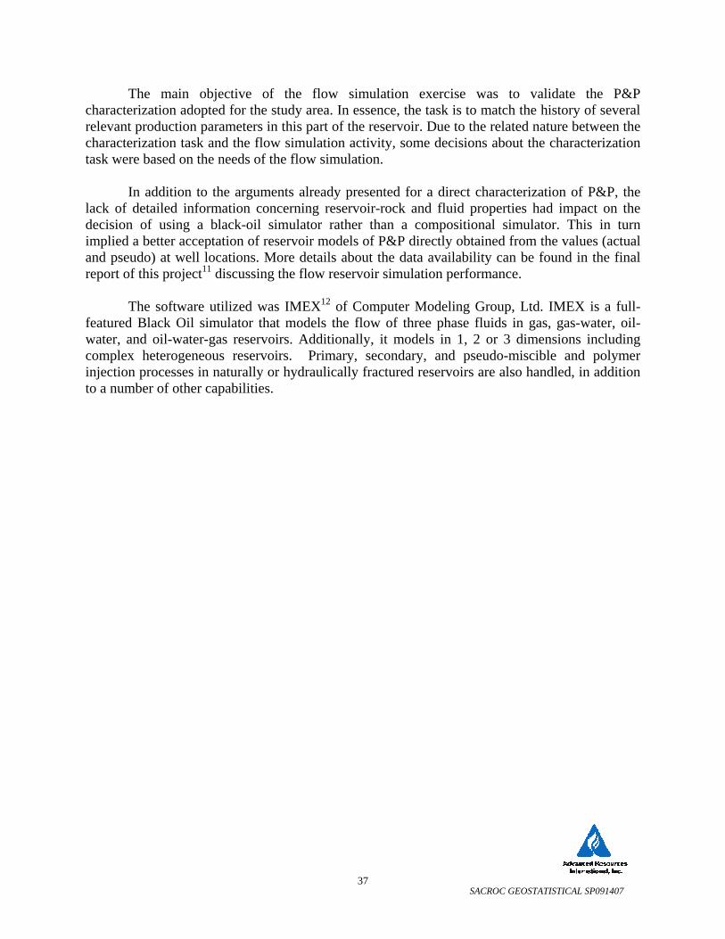
SACROC GEOSTATISTICAL SP091407
37
The main objective of the flow simulation exercise was to validate the P&P characterization adopted for the study area. In essence, the task is to match the history of several relevant production parameters in this part of the reservoir. Due to the related nature between the characterization task and the flow simulation activity, some decisions about the characterization task were based on the needs of the flow simulation.
In addition to the arguments already presented for a direct characterization of P&P, the
lack of detailed information concerning reservoir-rock and fluid properties had impact on the decision of using a black-oil simulator rather than a compositional simulator. This in turn implied a better acceptation of reservoir models of P&P directly obtained from the values (actual and pseudo) at well locations. More details about the data availability can be found in the final report of this project11 discussing the flow reservoir simulation performance.
The software utilized was IMEX12 of Computer Modeling Group, Ltd. IMEX is a full-
featured Black Oil simulator that models the flow of three phase fluids in gas, gas-water, oil-water, and oil-water-gas reservoirs. Additionally, it models in 1, 2 or 3 dimensions including complex heterogeneous reservoirs. Primary, secondary, and pseudo-miscible and polymer injection processes in naturally or hydraulically fractured reservoirs are also handled, in addition to a number of other capabilities.
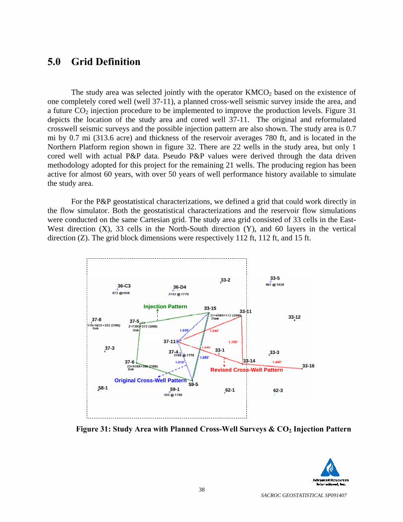
SACROC GEOSTATISTICAL SP091407
38
5.0 Grid Definition
The study area was selected jointly with the operator KMCO2 based on the existence of one completely cored well (well 37-11), a planned cross-well seismic survey inside the area, and a future CO2 injection procedure to be implemented to improve the production levels. Figure 31 depicts the location of the study area and cored well 37-11. The original and reformulated crosswell seismic surveys and the possible injection pattern are also shown. The study area is 0.7 mi by 0.7 mi (313.6 acre) and thickness of the reservoir averages 780 ft, and is located in the Northern Platform region shown in figure 32. There are 22 wells in the study area, but only 1 cored well with actual P&P data. Pseudo P&P values were derived through the data driven methodology adopted for this project for the remaining 21 wells. The producing region has been active for almost 60 years, with over 50 years of well performance history available to simulate the study area.
For the P&P geostatistical characterizations, we defined a grid that could work directly in
the flow simulator. Both the geostatistical characterizations and the reservoir flow simulations were conducted on the same Cartesian grid. The study area grid consisted of 33 cells in the East-West direction (X), 33 cells in the North-South direction (Y), and 60 layers in the vertical direction (Z). The grid block dimensions were respectively 112 ft, 112 ft, and 15 ft.
Figure 31: Study Area with Planned Cross-Well Surveys & CO2 Injection Pattern
Revised Cross-Well Pattern
Original Cross-Well Pattern
Injection Pattern
37-11
59-5
33-15
37-5
37-6
33-11
37-4 33-1
33-14
33-337-3
37-8
36-D436-C333-2
59-1 62-1 62-3
33-5
33-12
58-1
33-16Revised Cross-Well Pattern
Original Cross-Well Pattern
Injection Pattern
37-11
59-5
33-15
37-5
37-6
33-11
37-4 33-1
33-14
33-337-3
37-8
36-D436-C333-2
59-1 62-1 62-3
33-5
33-12
58-1
33-16Revised Cross-Well Pattern
Original Cross-Well Pattern
Injection Pattern
37-11
59-5
33-15
37-5
37-6
33-11
37-4 33-1
33-14
33-337-3
37-8
36-D436-C333-2
59-1 62-1 62-3
33-5
33-12
58-1
33-16
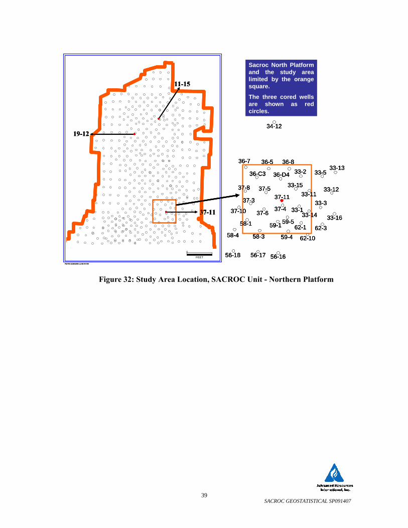
SACROC GEOSTATISTICAL SP091407
39
Figure 32: Study Area Location, SACROC Unit - Northern Platform
37-11
11-15
FEET
0
PETRA 2/28/2006 11:08:44 AM
19-12
Sacroc North Platform and the study area limited by the orange square.
The three cored wells are shown as red circles.
37-11
33-1
33-1133-12
33-13
33-14
33-15
33-16
33-2
33-3
33-5
34-12
36-536-7 36-8
36-C3 36-D4
37-10
37-337-4
37-5
37-6
37-8
56-1656-1756-18
58-1
58-358-4
59-1
59-4
59-562-1
62-10
62-3
37-11
11-15
FEET
0
PETRA 2/28/2006 11:08:44 AM
19-12
37-11
11-15
FEET
0
PETRA 2/28/2006 11:08:44 AM
19-12
Sacroc North Platform and the study area limited by the orange square.
The three cored wells are shown as red circles.
37-11
33-1
33-1133-12
33-13
33-14
33-15
33-16
33-2
33-3
33-5
34-12
36-536-7 36-8
36-C3 36-D4
37-10
37-337-4
37-5
37-6
37-8
56-1656-1756-18
58-1
58-358-4
59-1
59-4
59-562-1
62-10
62-3
37-11
33-1
33-1133-12
33-13
33-14
33-15
33-16
33-2
33-3
33-5
34-12
36-536-7 36-8
36-C3 36-D4
37-10
37-337-4
37-5
37-6
37-8
56-1656-1756-18
58-1
58-358-4
59-1
59-4
59-562-1
62-10
62-3
SACROC GEOSTATISTICAL SP091407
40
6.0 Sequential Gaussian Simulation
The goal of a geostatistical study is to provide the spatial distribution of the main reservoir parameters for simulating fluid flow and predicting performance of oil reservoirs. This information is used as the input data in the simulator. The purpose of the history matching study in a small region of the SACROC Unit is to validate the methodology for reservoir characterization developed in this project. The objective of the geostatistical simulation task was to represent the spatial distribution of porosity and permeability in the study area as a part of the combined procedure of characterization (data-driven/geostatistic) implemented in this project.
Calculations were carried out using the same reservoir volume as used for the fluid flow
simulation study and the same grid definition. For both porosity and permeability, the Sequential Gaussian Simulation technique was applied to interpolate data and to obtain multiple equiprobable realizations. Sequential Gaussian Simulation is the most popular and straightforward algorithm to generate possible spatial representations of a reservoir parameter. Simulation is executed sequentially using the conditional cumulative distribution function derived by solving a kriging system4,5,6,8. Kriging is a group of linear regression techniques to estimate a parameter value at an unsampled location (grid block) as a linear combination of the available samples in or near the grid block, such that the estimate has minimum error-variance4,5,6,8. More detailed information about Kriging methodologies can be found in references 4, 5, 6, and 8.
In addition, in the SGS algorithm, previously simulated points can be incorporated as
conditioning data. The number of conditioning data points (actual and simulated) included in the simulation of the reservoir parameter at any grid block is defined by a neighborhood search. The capacity to generate multiple representations is achieved by establishing different random paths for each realization. A random path is a sequence of unique visits to all grid locations that need to be provided with a simulated value. Since there are many possible combinations of visiting the grid, is possible to create different data configurations in each realization. Consequently, the algorithm is obligated to solve different kriging systems, and the resulting multiple images of the reservoir property will be different, although being statistically equiprobable4,5,6,8.
The simulation technique produces several possible realizations, and each realization
generally reproduces the characteristics of the input variable. Each simulated realization can be designed to honor (or not to honor) the constraining well data depending on the particular case study. The SGS procedure relies upon the multi-gaussian framework and generally requires a prior transformation of the information (from the raw set of samples to the Gaussian space) as well as a subsequent back transformation of the Gaussian simulated results to the original scale of data.
The utilized software was the Stanford Geostatistical Earth Modeling Software
(SGEMS)10 which is software for 3D geostatistical modeling that implements several classical geostatistics algorithms, as well as additional developments made at Stanford University. Its geostatistical routines includes Kriging, Cokriging, Sequential Gaussian Simulation, Sequential
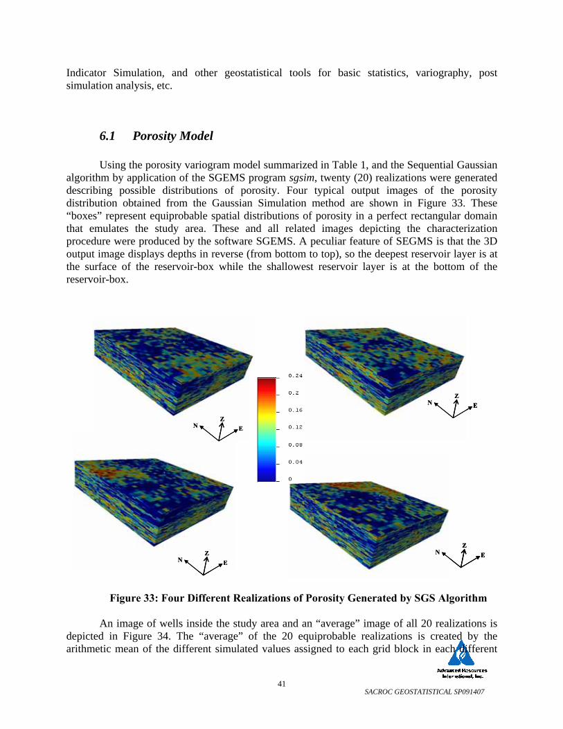
SACROC GEOSTATISTICAL SP091407
41
Indicator Simulation, and other geostatistical tools for basic statistics, variography, post simulation analysis, etc.
6.1 Porosity Model
Using the porosity variogram model summarized in Table 1, and the Sequential Gaussian algorithm by application of the SGEMS program sgsim, twenty (20) realizations were generated describing possible distributions of porosity. Four typical output images of the porosity distribution obtained from the Gaussian Simulation method are shown in Figure 33. These “boxes” represent equiprobable spatial distributions of porosity in a perfect rectangular domain that emulates the study area. These and all related images depicting the characterization procedure were produced by the software SGEMS. A peculiar feature of SEGMS is that the 3D output image displays depths in reverse (from bottom to top), so the deepest reservoir layer is at the surface of the reservoir-box while the shallowest reservoir layer is at the bottom of the reservoir-box.
Figure 33: Four Different Realizations of Porosity Generated by SGS Algorithm
An image of wells inside the study area and an “average” image of all 20 realizations is
depicted in Figure 34. The “average” of the 20 equiprobable realizations is created by the arithmetic mean of the different simulated values assigned to each grid block in each different
N EZ
N EZ N E
Z
N EZ
N EZ
N EZ
N EZ
N EZ N E
ZN E
Z
N EZ
N EZ
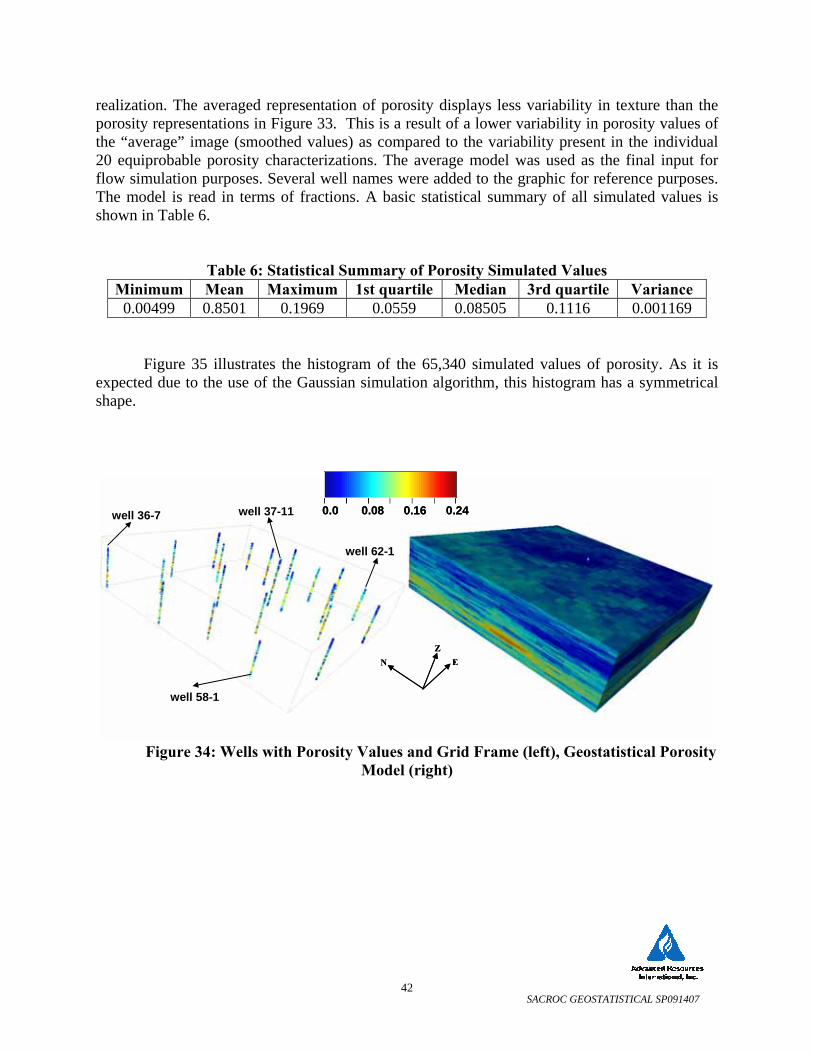
SACROC GEOSTATISTICAL SP091407
42
realization. The averaged representation of porosity displays less variability in texture than the porosity representations in Figure 33. This is a result of a lower variability in porosity values of the “average” image (smoothed values) as compared to the variability present in the individual 20 equiprobable porosity characterizations. The average model was used as the final input for flow simulation purposes. Several well names were added to the graphic for reference purposes. The model is read in terms of fractions. A basic statistical summary of all simulated values is shown in Table 6.
Table 6: Statistical Summary of Porosity Simulated Values Minimum Mean Maximum 1st quartile Median 3rd quartile Variance
0.00499 0.8501 0.1969 0.0559 0.08505 0.1116 0.001169
Figure 35 illustrates the histogram of the 65,340 simulated values of porosity. As it is expected due to the use of the Gaussian simulation algorithm, this histogram has a symmetrical shape.
Figure 34: Wells with Porosity Values and Grid Frame (left), Geostatistical Porosity Model (right)
EZ
N
well 37-11
well 62-1
well 36-7
well 58-1
0.0 0.08 0.16 0.24
EZ
N EZ
N
well 37-11
well 62-1
well 36-7
well 58-1
0.0 0.08 0.16 0.240.0 0.08 0.16 0.24

SACROC GEOSTATISTICAL SP091407
43
Figure 35: Histogram of Porosity Simulated Values (“Average” Porosity Model)
6.2 Permeability Model Based on the assumed correlation between porosity and logarithm of permeability, the
Sequential Gaussian algorithm was adopted again to simulate the logarithm of permeability now supplemented by the model adopted for porosity in the study area as parameter guide. For cosimulation tasks, SGEMS10 provides the program cosgsim which allows simulating a Gaussian variable accounting for secondary information. As discussed in SGEMS manual10, the program cosgsim permits a selection of either solving a full cokriging system, or only retaining the co-located secondary datum at each location and assuming one of two Markov models that present different considerations about the existing crossed correlation between parameters4,5,6,8,10. The approach used in this study was to utilize the dependence of the secondary variable on the primary variable, limited only to the co-located primary variable, with the cross-variogram proportional to the variogram of the primary variable. This option also requires a correlation coefficient value between the variable to be simulated (primary) and the variable used as guide (secondary). Based on the window averaged analysis developed between logarithm of permeability and porosity (Table 1.5), a value of 0.725 was adopted when 20 different realizations of logarithm of permeability were generated.
Figure 36 shows the averaged model of logarithm of permeability jointly the wells
located in the study area and their corresponding values of logarithm of permeability. As a final model of permeability, each value of Log10(K0) was back-transformed by using the exponential function (with base 10) given by f(x) = 10x. In Figure 37, the final model of permeability and wells with their corresponding values of original permeability is shown. This permeability model
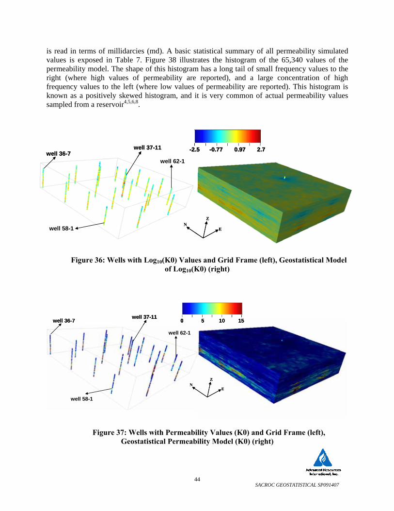
SACROC GEOSTATISTICAL SP091407
44
is read in terms of millidarcies (md). A basic statistical summary of all permeability simulated values is exposed in Table 7. Figure 38 illustrates the histogram of the 65,340 values of the permeability model. The shape of this histogram has a long tail of small frequency values to the right (where high values of permeability are reported), and a large concentration of high frequency values to the left (where low values of permeability are reported). This histogram is known as a positively skewed histogram, and it is very common of actual permeability values sampled from a reservoir4,5,6,8.
Figure 36: Wells with Log10(K0) Values and Grid Frame (left), Geostatistical Model
of Log10(K0) (right)
Figure 37: Wells with Permeability Values (K0) and Grid Frame (left),
Geostatistical Permeability Model (K0) (right)
Z
EN
well 37-11
well 62-1well 36-7
well 58-1
-2.5 -0.77 0.97 2.7
Z
EN
Z
EN
well 37-11
well 62-1well 36-7
well 58-1
-2.5 -0.77 0.97 2.7-2.5 -0.77 0.97 2.7
Z
EN
well 37-11
well 62-1
well 36-7
well 58-1
0 5 10 15
Z
EN
Z
EN
well 37-11
well 62-1
well 36-7
well 58-1
0 5 10 150 5 10 15

SACROC GEOSTATISTICAL SP091407
45
Figure 38: Histogram of Permeability Simulated Values
Table 7: Statistical Summary Of Permeability Simulated Values Minimum Mean Maximum 1st quartile Median 3rd quartile Variance
0.05835 2.7438 70.9235 1.2954 2.1131 3.4973 5.020
Figure 39 is a crossplot of simulated values of permeability vs. simulated values of porosity. On the left is the logarithm of permeability and on the right is the direct permeability. As can be seen in both graphics, the good alignment of simulated values demonstrates the expected correlation between these parameters. The corresponding correlation coefficients obtained from both crossplots are 0.77 for Log10(K0), and 0.67 for K0. Thus, the cosimulation algorithm generated an improved correlation coefficient value (0.77) in comparison with the value originally proposed (0.725), but is still of an equivalent magnitude to those correlation coefficient values found when logarithm of permeability and porosity were crossed for different window averaged samples (see Table 2). The value of 0.67 is obtained directly from the back transformed permeability model. It is a significant value when compared to the original correlation coefficients calculated for core porosity and permeability data sampled foot by foot (0.20, 0.12, and 0.21 for well 11-15, well 19-12, and well 37-11 respectively). However, these correlation values were considered of limited usefulness due to the origin of the data (foot by foot sampled data) if compared with the support volume of the grid blocks (112’ x 112’ x 15’) where simulated values are assigned. Additionally, they were directly calculated without any consideration of the logarithmic relation frequently found between these two parameters.
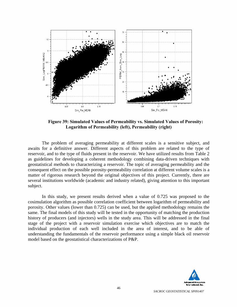
SACROC GEOSTATISTICAL SP091407
46
Figure 39: Simulated Values of Permeability vs. Simulated Values of Porosity: Logarithm of Permeability (left), Permeability (right)
The problem of averaging permeability at different scales is a sensitive subject, and
awaits for a definitive answer. Different aspects of this problem are related to the type of reservoir, and to the type of fluids present in the reservoir. We have utilized results from Table 2 as guidelines for developing a coherent methodology combining data-driven techniques with geostatistical methods to characterizing a reservoir. The topic of averaging permeability and the consequent effect on the possible porosity-permeability correlation at different volume scales is a matter of rigorous research beyond the original objectives of this project. Currently, there are several institutions worldwide (academic and industry related), giving attention to this important subject.
In this study, we present results derived when a value of 0.725 was proposed to the
cosimulation algorithm as possible correlation coefficient between logarithm of permeability and porosity. Other values (lower than 0.725) can be used, but the applied methodology remains the same. The final models of this study will be tested in the opportunity of matching the production history of producers (and injectors) wells in the study area. This will be addressed in the final stage of the project with a reservoir simulation exercise which objectives are to match the individual production of each well included in the area of interest, and to be able of understanding the fundamentals of the reservoir performance using a simple black oil reservoir model based on the geostatistical characterizations of P&P.
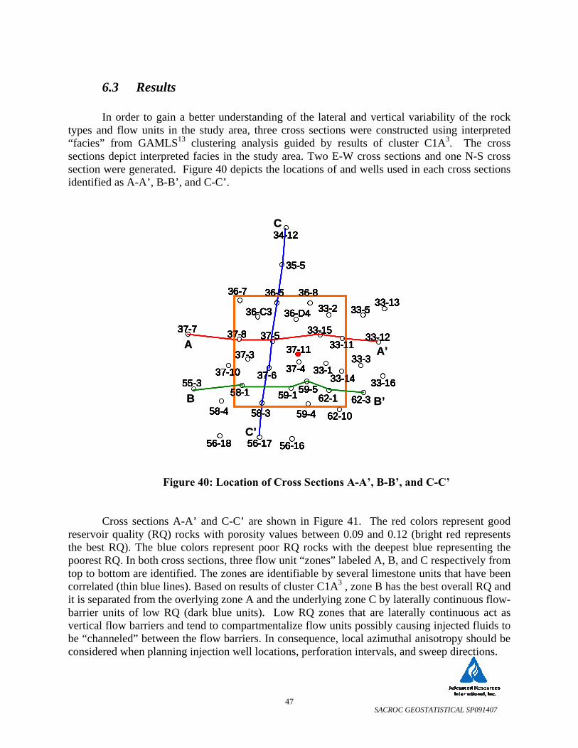
SACROC GEOSTATISTICAL SP091407
47
6.3 Results
In order to gain a better understanding of the lateral and vertical variability of the rock types and flow units in the study area, three cross sections were constructed using interpreted “facies” from GAMLS13 clustering analysis guided by results of cluster C1A3. The cross sections depict interpreted facies in the study area. Two E-W cross sections and one N-S cross section were generated. Figure 40 depicts the locations of and wells used in each cross sections identified as A-A’, B-B’, and C-C’.
Figure 40: Location of Cross Sections A-A’, B-B’, and C-C’
Cross sections A-A’ and C-C’ are shown in Figure 41. The red colors represent good
reservoir quality (RQ) rocks with porosity values between 0.09 and 0.12 (bright red represents the best RQ). The blue colors represent poor RQ rocks with the deepest blue representing the poorest RQ. In both cross sections, three flow unit “zones” labeled A, B, and C respectively from top to bottom are identified. The zones are identifiable by several limestone units that have been correlated (thin blue lines). Based on results of cluster C1A3 , zone B has the best overall RQ and it is separated from the overlying zone A and the underlying zone C by laterally continuous flow-barrier units of low RQ (dark blue units). Low RQ zones that are laterally continuous act as vertical flow barriers and tend to compartmentalize flow units possibly causing injected fluids to be “channeled” between the flow barriers. In consequence, local azimuthal anisotropy should be considered when planning injection well locations, perforation intervals, and sweep directions.
37-11
33-1
33-1133-12
33-13
33-14
33-15
33-16
33-2
33-3
33-5
34-12
36-536-7 36-8
36-C3 36-D4
37-10
37-337-4
37-5
37-6
37-8
56-1656-1756-18
58-1
58-358-459-1
59-4
59-562-1
62-10
62-3
35-5
37-7
37-11
33-1
33-1133-12
33-13
33-14
33-15
33-16
33-2
33-3
33-5
34-12
36-536-7 36-8
36-C3 36-D4
37-10
37-337-4
37-5
37-6
37-8
56-1656-1756-18
58-1
58-358-459-1
59-4
59-562-1
62-10
62-3
35-5
37-7
55-3
37-11
33-1
33-1133-12
33-13
33-14
33-15
33-16
33-2
33-3
33-5
34-12
36-536-7 36-8
36-C3 36-D4
37-10
37-337-4
37-5
37-6
37-8
56-1656-1756-18
58-1
58-358-459-1
59-4
59-562-1
62-10
62-3
35-5
37-7
37-11
33-1
33-1133-12
33-13
33-14
33-15
33-16
33-2
33-3
33-5
34-12
36-536-7 36-8
36-C3 36-D4
37-10
37-337-4
37-5
37-6
37-8
56-1656-1756-18
58-1
58-358-459-1
59-4
59-562-1
62-10
62-3
35-5
37-7
55-3
A A’
B B’
C
C’
37-11
33-1
33-1133-12
33-13
33-14
33-15
33-16
33-2
33-3
33-5
34-12
36-536-7 36-8
36-C3 36-D4
37-10
37-337-4
37-5
37-6
37-8
56-1656-1756-18
58-1
58-358-459-1
59-4
59-562-1
62-10
62-3
35-5
37-7
37-11
33-1
33-1133-12
33-13
33-14
33-15
33-16
33-2
33-3
33-5
34-12
36-536-7 36-8
36-C3 36-D4
37-10
37-337-4
37-5
37-6
37-8
56-1656-1756-18
58-1
58-358-459-1
59-4
59-562-1
62-10
62-3
35-5
37-7
55-3
37-11
33-1
33-1133-12
33-13
33-14
33-15
33-16
33-2
33-3
33-5
34-12
36-536-7 36-8
36-C3 36-D4
37-10
37-337-4
37-5
37-6
37-8
56-1656-1756-18
58-1
58-358-459-1
59-4
59-562-1
62-10
62-3
35-5
37-7
37-11
33-1
33-1133-12
33-13
33-14
33-15
33-16
33-2
33-3
33-5
34-12
36-536-7 36-8
36-C3 36-D4
37-10
37-337-4
37-5
37-6
37-8
56-1656-1756-18
58-1
58-358-459-1
59-4
59-562-1
62-10
62-3
35-5
37-7
55-3
A A’
B B’
C
C’

SACROC GEOSTATISTICAL SP091407
48
The cross sections in Figure 41 can be used to analyze the lateral continuity of zones A, B, and C. In cross section C-C’, the individual zones from well to well are quite similar. This is particularly evident in zone B where better RQ units are predominant. This can be related to the pattern of deposition of SACROC sediments which were controlled by a structural axis with dominant N-S trend. This setting also explains why in E-W cross section A-A’ it is more difficult to find stratigraphic similarity between the same zones of different wells or among the individual flow units within the zones. In cross section B-B’ (here omitted), approximate positions of the zones A, B, and C were easily found at well 59-1 but, in general, the zones and the individual flow units within the zones are less well-defined in this southern part of the study area3. The complete groups of wells included in both cross sections are analyzed in reference 3.
Figure 41: Cross Section C-C’ (left) and Cross Section A-A’ (right) Showing Rock
Types Probabilistic Representation Figure 42, depicts two cross sections of the porosity model (left) and the permeability
model (right) across the study area. The model cross sections are the cross section N° 20 (E-W, approximate A-A’ location), and the cross section N° 11 (N-S, approximate C-C’ location). Scale for porosity is in fractions and permeability in millidarcies (md).
low por & low perm flow barriers
low por & low perm flow barriers
low por & low perm flow barriers
low por & low perm flow barriers
low por & low perm flow barriers
low por & low perm flow barriers
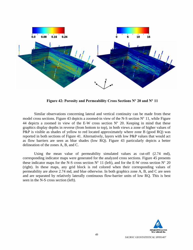
SACROC GEOSTATISTICAL SP091407
49
Figure 42: Porosity and Permeability Cross Sections N° 20 and N° 11
Similar observations concerning lateral and vertical continuity can be made from these
model cross sections. Figure 43 depicts a zoomed-in view of the N-S section N° 11, while Figure 44 depicts a zoomed in view of the E-W cross section N° 20. Keeping in mind that these graphics display depths in reverse (from bottom to top), in both views a zone of higher values of P&P is visible as shades of yellow to red located approximately where zone B (good RQ) was reported in both sections of Figure 41. Alternatively, layers with low P&P values that would act as flow barriers are seen as blue shades (low RQ). Figure 43 particularly depicts a better delineation of the zones A, B, and C.
Using the mean value of permeability simulated values as cut-off (2.74 md),
corresponding indicator maps were generated for the analyzed cross sections. Figure 45 presents these indicator maps for the N-S cross section N° 11 (left), and for the E-W cross section N° 20 (right). In these maps, any grid block is red colored when their corresponding values of permeability are above 2.74 md, and blue otherwise. In both graphics zone A, B, and C are seen and are separated by relatively laterally continuous flow-barrier units of low RQ. This is best seen in the N-S cross section (left).
Z
EN
0 5 10 150.0 0.08 0.16 0.24
Z
EN
Z
EN
0 5 10 150 5 10 150.0 0.08 0.16 0.240.0 0.08 0.16 0.24
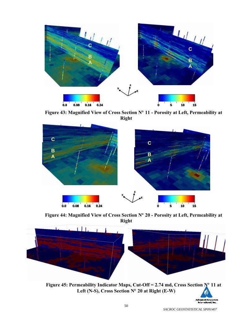
SACROC GEOSTATISTICAL SP091407
50
Figure 43: Magnified View of Cross Section N° 11 - Porosity at Left, Permeability at
Right
Figure 44: Magnified View of Cross Section N° 20 - Porosity at Left, Permeability at
Right
Figure 45: Permeability Indicator Maps, Cut-Off = 2.74 md, Cross Section N° 11 at Left (N-S), Cross Section N° 20 at Right (E-W)
0 5 10 150.0 0.08 0.16 0.24
Z
EN
0 5 10 150 5 10 150.0 0.08 0.16 0.240.0 0.08 0.16 0.24
Z
EN
Z
EN
C B A
C B A
0 5 10 150.0 0.08 0.16 0.24
Z
EN
0 5 10 150 5 10 150.0 0.08 0.16 0.240.0 0.08 0.16 0.24
Z
EN
Z
EN
C B A
C B A
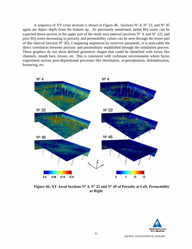
SACROC GEOSTATISTICAL SP091407
51
A sequence of XY cross sections is shown in Figure 46. Sections N° 4, N° 22, and N° 45 again are depict depth from the bottom up. As previously mentioned, better RQ zones can be expected down-section in the upper part of the study area interval (sections N° 4, and N° 22), and poor RQ zones decreasing in porosity and permeability values can be seen through the lower part of this interval (section N° 45). Comparing sequences by reservoir parameter, it is noticeable the direct correlation between porosity and permeability established through the simulation process. These graphics do not show defined geometric shapes that could be identified with facies like channels, mouth bars, levees, etc. This is consistent with carbonate environments where facies experiment serious post-depositional processes like dissolution, re-precipitation, dolomitization, fracturing, etc.
Figure 46: XY Areal Sections N° 4, N° 22 and N° 45 of Porosity at Left, Permeability at Right
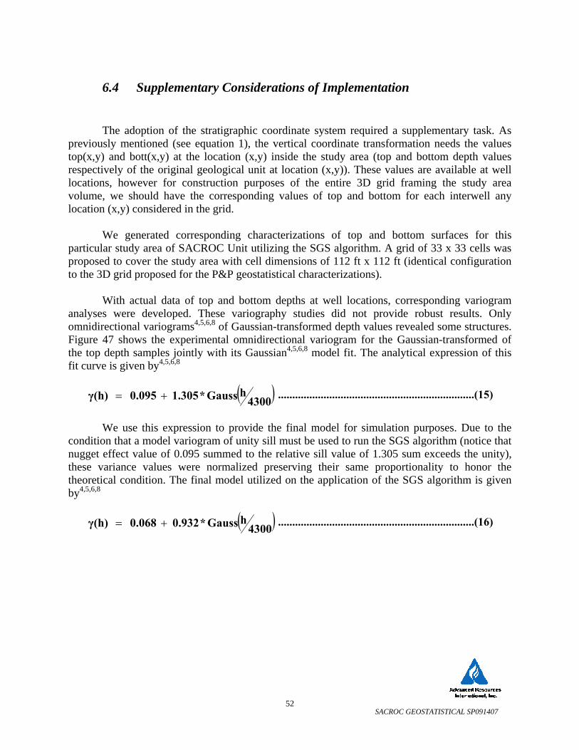
SACROC GEOSTATISTICAL SP091407
52
6.4 Supplementary Considerations of Implementation
The adoption of the stratigraphic coordinate system required a supplementary task. As previously mentioned (see equation 1), the vertical coordinate transformation needs the values top(x,y) and bott(x,y) at the location (x,y) inside the study area (top and bottom depth values respectively of the original geological unit at location (x,y)). These values are available at well locations, however for construction purposes of the entire 3D grid framing the study area volume, we should have the corresponding values of top and bottom for each interwell any location (x,y) considered in the grid.
We generated corresponding characterizations of top and bottom surfaces for this
particular study area of SACROC Unit utilizing the SGS algorithm. A grid of 33 x 33 cells was proposed to cover the study area with cell dimensions of 112 ft x 112 ft (identical configuration to the 3D grid proposed for the P&P geostatistical characterizations).
With actual data of top and bottom depths at well locations, corresponding variogram
analyses were developed. These variography studies did not provide robust results. Only omnidirectional variograms4,5,6,8 of Gaussian-transformed depth values revealed some structures. Figure 47 shows the experimental omnidirectional variogram for the Gaussian-transformed of the top depth samples jointly with its Gaussian4,5,6,8 model fit. The analytical expression of this fit curve is given by4,5,6,8
( ) 4300hGauss *1.305 0.095 γ(h) += .....................................................................(15)
We use this expression to provide the final model for simulation purposes. Due to the
condition that a model variogram of unity sill must be used to run the SGS algorithm (notice that nugget effect value of 0.095 summed to the relative sill value of 1.305 sum exceeds the unity), these variance values were normalized preserving their same proportionality to honor the theoretical condition. The final model utilized on the application of the SGS algorithm is given by4,5,6,8
( ) 4300hGauss *0.932 0.068 γ(h) += .....................................................................(16)
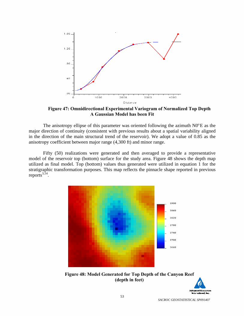
SACROC GEOSTATISTICAL SP091407
53
Figure 47: Omnidirectional Experimental Variogram of Normalized Top Depth A Gaussian Model has been Fit
The anisotropy ellipse of this parameter was oriented following the azimuth N0°E as the
major direction of continuity (consistent with previous results about a spatial variability aligned in the direction of the main structural trend of the reservoir). We adopt a value of 0.85 as the anisotropy coefficient between major range (4,300 ft) and minor range.
Fifty (50) realizations were generated and then averaged to provide a representative
model of the reservoir top (bottom) surface for the study area. Figure 48 shows the depth map utilized as final model. Top (bottom) values thus generated were utilized in equation 1 for the stratigraphic transformation purposes. This map reflects the pinnacle shape reported in previous reports3,14.
Figure 48: Model Generated for Top Depth of the Canyon Reef (depth in feet)
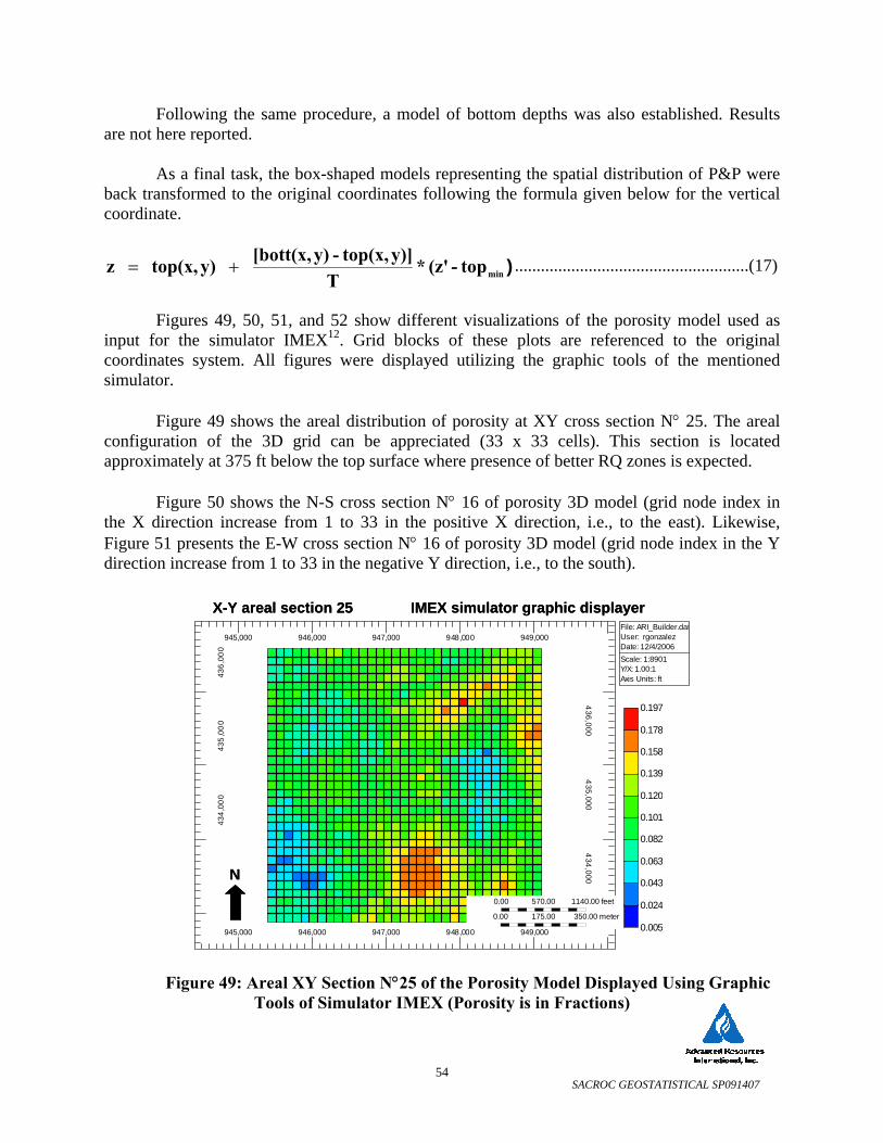
SACROC GEOSTATISTICAL SP091407
54
Following the same procedure, a model of bottom depths was also established. Results are not here reported.
As a final task, the box-shaped models representing the spatial distribution of P&P were
back transformed to the original coordinates following the formula given below for the vertical coordinate.
)mintop - (z'*T
y)]top(x, - y)[bott(x, y)top(x, z += ......................................................(17)
Figures 49, 50, 51, and 52 show different visualizations of the porosity model used as
input for the simulator IMEX12. Grid blocks of these plots are referenced to the original coordinates system. All figures were displayed utilizing the graphic tools of the mentioned simulator.
Figure 49 shows the areal distribution of porosity at XY cross section N° 25. The areal
configuration of the 3D grid can be appreciated (33 x 33 cells). This section is located approximately at 375 ft below the top surface where presence of better RQ zones is expected.
Figure 50 shows the N-S cross section N° 16 of porosity 3D model (grid node index in
the X direction increase from 1 to 33 in the positive X direction, i.e., to the east). Likewise, Figure 51 presents the E-W cross section N° 16 of porosity 3D model (grid node index in the Y direction increase from 1 to 33 in the negative Y direction, i.e., to the south).
Figure 49: Areal XY Section N°25 of the Porosity Model Displayed Using Graphic Tools of Simulator IMEX (Porosity is in Fractions)
945,000 946,000 947,000 948,000 949,000
945,000 946,000 947,000 948,000 949,000
434
,000
435,
000
436
,000
434,000
435,000
436,000
0.00 570.00 1140.00 feet
0.00 175.00 350.00 meters
File: ARI_Builder.datUser: rgonzalezDate: 12/4/2006Scale: 1:8901Y/X: 1.00:1Axis Units: ft
0.005
0.024
0.043
0.063
0.082
0.101
0.120
0.139
0.158
0.178
0.197
N
X-Y areal section 25 IMEX simulator graphic displayer
945,000 946,000 947,000 948,000 949,000
945,000 946,000 947,000 948,000 949,000
434
,000
435,
000
436
,000
434,000
435,000
436,000
0.00 570.00 1140.00 feet
0.00 175.00 350.00 meters
File: ARI_Builder.datUser: rgonzalezDate: 12/4/2006Scale: 1:8901Y/X: 1.00:1Axis Units: ft
0.005
0.024
0.043
0.063
0.082
0.101
0.120
0.139
0.158
0.178
0.197
NN
X-Y areal section 25 IMEX simulator graphic displayer
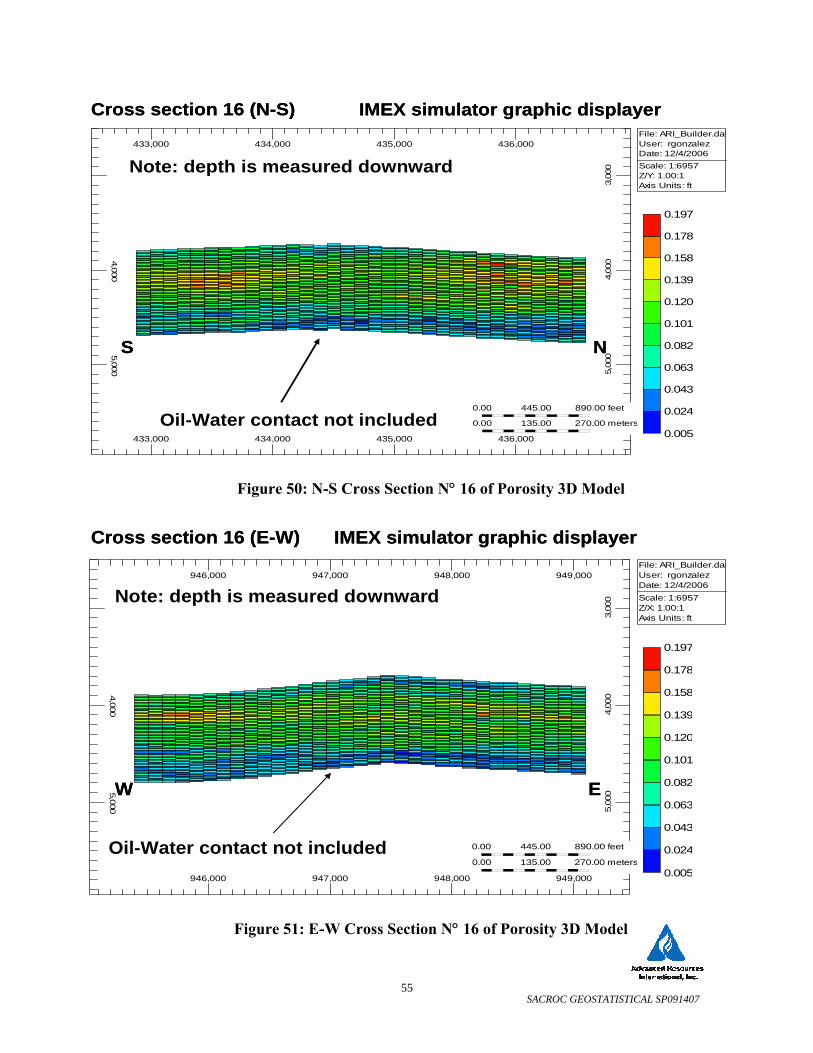
SACROC GEOSTATISTICAL SP091407
55
Figure 50: N-S Cross Section N° 16 of Porosity 3D Model
Figure 51: E-W Cross Section N° 16 of Porosity 3D Model
946,000 947,000 948,000 949,000
946,000 947,000 948,000 949,000
4,0005,000
3,00
04,
000
5,00
0
0.00 445.00 890.00 feet
0.00 135.00 270.00 meters
File: ARI_Builder.datUser: rgonzalezDate: 12/4/2006Scale: 1:6957Z/X: 1.00:1Axis Units: ft
0.005
0.024
0.043
0.063
0.082
0.101
0.120
0.139
0.158
0.178
0.197
Cross section 16 (E-W)
Oil-Water contact not included
Note: depth is measured downward
EW
IMEX simulator graphic displayer
946,000 947,000 948,000 949,000
946,000 947,000 948,000 949,000
4,0005,000
3,00
04,
000
5,00
0
0.00 445.00 890.00 feet
0.00 135.00 270.00 meters
File: ARI_Builder.datUser: rgonzalezDate: 12/4/2006Scale: 1:6957Z/X: 1.00:1Axis Units: ft
0.005
0.024
0.043
0.063
0.082
0.101
0.120
0.139
0.158
0.178
0.197
Cross section 16 (E-W)
Oil-Water contact not included
Note: depth is measured downward
EW EW
IMEX simulator graphic displayer
433,000 434,000 435,000 436,000
433,000 434,000 435,000 436,000
4,0005,000
3,00
04,
000
5,00
0
0.00 445.00 890.00 feet
0.00 135.00 270.00 meters
File: ARI_Builder.datUser: rgonzalezDate: 12/4/2006Scale: 1:6957Z/Y: 1.00:1Axis Units: ft
0.005
0.024
0.043
0.063
0.082
0.101
0.120
0.139
0.158
0.178
0.197
Cross section 16 (N-S)
Oil-Water contact not included
Note: depth is measured downward
NS
IMEX simulator graphic displayer
433,000 434,000 435,000 436,000
433,000 434,000 435,000 436,000
4,0005,000
3,00
04,
000
5,00
0
0.00 445.00 890.00 feet
0.00 135.00 270.00 meters
File: ARI_Builder.datUser: rgonzalezDate: 12/4/2006Scale: 1:6957Z/Y: 1.00:1Axis Units: ft
0.005
0.024
0.043
0.063
0.082
0.101
0.120
0.139
0.158
0.178
0.197
Cross section 16 (N-S)
Oil-Water contact not included
Note: depth is measured downward
NS NS
IMEX simulator graphic displayer
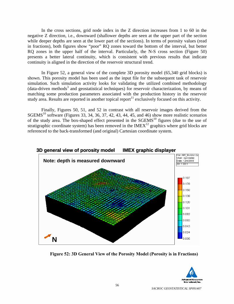
SACROC GEOSTATISTICAL SP091407
56
In the cross sections, grid node index in the Z direction increases from 1 to 60 in the negative Z direction, i.e., downward (shallower depths are seen at the upper part of the section while deeper depths are seen at the lower part of the sections). In terms of porosity values (read in fractions), both figures show “poor” RQ zones toward the bottom of the interval, but better RQ zones in the upper half of the interval. Particularly, the N-S cross section (Figure 50) presents a better lateral continuity, which is consistent with previous results that indicate continuity is aligned in the direction of the reservoir structural trend.
In Figure 52, a general view of the complete 3D porosity model (65,340 grid blocks) is
shown. This porosity model has been used as the input file for the subsequent task of reservoir simulation. Such simulation activity looks for validating the utilized combined methodology (data-driven methods3 and geostatistical techniques) for reservoir characterization, by means of matching some production parameters associated with the production history in the reservoir study area. Results are reported in another topical report11 exclusively focused on this activity.
Finally, Figures 50, 51, and 52 in contrast with all reservoir images derived from the
SGEMS10 software (Figures 33, 34, 36, 37, 42, 43, 44, 45, and 46) show more realistic scenarios of the study area. The box-shaped effect presented in the SGEMS10 figures (due to the use of stratigraphic coordinate system) has been removed in the IMEX12 graphics where grid blocks are referenced to the back-transformed (and original) Cartesian coordinate system.
Figure 52: 3D General View of the Porosity Model (Porosity is in Fractions)
N
3D general view of porosity model
Note: depth is measured downward
IMEX graphic displayer
N
3D general view of porosity model
Note: depth is measured downward
IMEX graphic displayer
SACROC GEOSTATISTICAL SP091407
57
7.0 Conclusions
1. An integrated Clustering/Geostatistical approach for 3D Reservoir Characterization has been tested successfully in the Pennsylvanian-Permian reef carbonates (Cisco and Canyon Formations) of a subregion of the SACROC Unit, Horseshoe Atoll, Permian Basin, Texas.
2. The integrated Clustering/Geostatistical approach was successfully tested in a relevant area of the
SACROC Unit Platform. This approach was constituted by a two-step pattern recognition procedure (soft-computing) combined with the application of geostatistical algorithms. The soft-computing procedure permitted the efficient generation of core-scale P&P profiles and rock types at well locations where no core data existed populating this way all wells inside the studied area. These core-scale estimates of P&P and rock types facilitated direct application of geostatistical methods to build 3D reservoir models.
3. Variography studies could be performed using directly the vertical profiles of core porosity and
permeability set on each region well (both actual core data, and estimated values of porosity and permeability by soft-computing clustering methods). These variogram analyses were utilized to describe patterns of spatial variability of these reservoir parameters.
4. Different scales of variability can be seen in variograms of core porosity and permeability (actual and
estimated values) in the reef-carbonate depositional environment of SACROC. 5. The variogram analysis conducted to evaluate spatial continuity of core porosity and permeability (actual
and estimated values) in the vertical direction indicated spatial behaviors associated with geologic cyclicity. Cyclicity could not be appreciated in horizontal variograms.
6. Both variography studies, vertical and horizontal, conducted to variogram models using an isotropic nugget
structure and two structures with geometric anisotropy reflecting an intermediate and a global scale. These different scales were mainly associated to complex patterns of sediment deposition of the reservoir, and constructional characteristics of the SACROC limestone reef (structural factors).
7. Variogram analysis of rock types (derived by the application of the soft-computing methodology) aided to
model the spatial continuity of core porosity and permeability (actual and estimated values). These “lithologic” controls helped to elucidate spatial patterns where direct variograms of P&P were failing.
8. The porosity and permeability characterizations were developed in a grid that could work directly in the
flow simulator. In consequence, the geostatistical characterizations and posterior reservoir flow simulations were both conducted on the same Cartesian grid.
9. A direct application of SGS algorithms to actual and estimate values of core porosity and permeability lead
to 3D models of porosity and permeability that honored the raw data and honored quite closely the division of the carbonate section into "good" and "poor" RQ zones.
10. From the qualitative and quantitative point of views, a porosity model highly trustworthy was developed
with this combined methodology (average porosity of this heterogeneous model was 8.5%). 11. A highly reliable permeability model was generated from the qualitative viewpoint (identification and
characterization of geological trends and realistic heterogeneities); however, estimated permeability values were considered possibly undervalued (average horizontal permeability of this characterization was 2.74 mD). This fact is attributable to the smoothing effect inherent to those utilized algorithms based on Gaussian assumptions.
12. The direct application of conventional geostatistical algorithms in this work was favored by the
considerable quantity of information present on wells inside the studied region. This definitively was a
SACROC GEOSTATISTICAL SP091407
58
consequence of the application of advanced pattern recognition techniques that provided likely rock types and reliable estimates of P&P (with high vertical resolution) at all well locations.
13. Reciprocally, the utilization of geostatistical algorithms allowed the three-dimensional extension, of those
results derived from the application of the clustering methodology, to the whole volume of the area under study. This “symbiotic” interaction between these two mathematical approaches strengthens their corresponding possibilities of applicability offering a significant advance over their individual uses, and other conventional methodologies.
14. This combined approach -application of advanced pattern recognition techniques and geostatistical
algorithms- has the potential of being applied successfully either on other subregions of SACROC or entirely on the whole SACROC unit. Besides, both mathematical approaches can make use of the seismic data (either individually or jointly), where the existence and quality of this type of information allows it. Besides, we do believe that this combined approach can be applied successfully to other reservoir types under a minimum of proper conditions of information availability.
SACROC GEOSTATISTICAL SP091407
59
8.0 References
1. Reeves, S.R., Mohaghegh, S.D., Fairborn, J.W., and Luca, G.: “Feasibility Assessment of a New Approach for Integrating Multiscale Data for High-Resolution Reservoir Characterization”, paper SPE 77795 presented at the SPE Annual Technical Conference and Exhibition, San Antonio, Texas, Sept. 29 - Oct.2, 2002
2. Steen, J.W., and Reeves, S.R.: “Development, Testing and Validation of a Neural Model to Predict Porosity and Permeability from Well Logs, Grayburg Formation, McElroy Field, West Texas”, Topical Report, U.S. Department of Energy, Contract Number DE-FC26-01BC15357, July 2003.
3. González, R.J., Reeves, S.R., and Eslinger, E.: “Predicting Porosity and Permeability for the Canyon Formation, SACROC Unit (Kelly-Snyder Field), Using the Geologic Analysis via Maximum Likelihood System”, Topical Report for U.S. Department of Energy, Contract Number DE-FC26-04NT15514, September, 2007.
4. Deutsch, C.V.: “Geostatistical Reservoir Modeling”, first edition, Oxford University Press, 2002.
5. Deutsch, C.V., and Journel, A.G.: “GSLIB. Geostatistical Software Library and User’s Guide”, second edition, Oxford University Press, 1998.
6. Goovaerts, P.: “Geostatistics for Natural Resources Evaluation”, first edition, Oxford University Press, 1997.
7. Yarus, J.M. and Chambers, R.L.: “Practical Geostatistics—An Armchair Overview for Petroleum Reservoir Engineers”. JPT (November 2006) 78.
8. Isaaks, E.H., and Srivastava, R.M.: “An Introduction to Applied Geostatistics”, first edition, Oxford University Press, 1989.
9. Gringarten, E., and Deutsch, C.V.: “Variogram Interpretation and Modeling”, Mathematical Geology, Vol. 33, Number 4, 2001.
10. Remy, N.: “SGEMS: The Stanford Geostatistical Earth Modeling Software. User’s Manual”, http://sgems.sourceforge.net/doc/sgems_manual.pdf, May 2004.
11. Schepers, K., Gonzalez, R.J., and Reeves, S.R.: “Reservoir Simulation of the Canyon Formation, SACROC Unit (Kelly-Snyder Field), Topical Report prepared for U.S. Department of Energy, Contract Number DE-FC26-04NT15514, September 2007.
12. “IMEX. Advanced Oil/Gas Reservoir Simulator. 2007 User’s Guide”, Computer Modelling Group Ltd., 2007.
13. Eslinger, E.: “GAMLS (Geologic Analysis via Maximum Likelihood System). User’s Manual”, ericgeoscience.com, Eric Geoscience, Inc., 2000.
14. Raines, M., Dobitz, J.K., and Wehner, S.C.: “A Review of the Pennsylvanian SACROC Unit”, paper presented at West Texas Geological Society Fall Symposium, Midland, TX, Oct. 24-25, 2001.
SACROC GEOSTATISTICAL SP091407
60
9.0 List of Acronyms and Abbreviations bott(x,y) = bottom depth at location (x,y) DT = delta time GR = gamma ray Gauss = Gaussian variogram model K0 = permeability along master orientation lineK90 = permeability at 90 degrees from K0 line KV = vertical permeability NPHI = neutron porosity P&P = porosity and permeability RHOB = bulk density RQ = reservoir quality Sph = spherical variogram model T = any meaningful thickness of the reservoir top(x,y) = top depth at location (x,y) topmin = minimum value of sampled top values
γ(h) = variogram model (x’,y’,z’) = transformed stratigraphic coordinates