geospatial technologies to improve urban energy …...geospatial technologies to improve urban...

Remote Sens. 2011, 3, 1380-1405; doi:10.3390/rs3071380

Remote Sensing ISSN 2072-4292

www.mdpi.com/journal/remotesensing

Article

Geospatial Technologies to Improve Urban Energy Efficiency

Geoffrey J. Hay 1,*, Christopher Kyle

1, Bharanidharan Hemachandran

1, Gang Chen

1,

Mir Mustafizur Rahman 1, Tak S. Fung

2 and Joseph L. Arvai

3,4

1 Foothills Facility for Remote Sensing and GIScience, Department of Geography, University of

Calgary, 2500 University Drive N.W., Calgary, AB T2N 1N4, Canada;

E-Mails: [email protected] (C.D.K.); [email protected] (B.H.);

[email protected] (G.C.); [email protected] (M.M.R.) 2 Information Technologies, University of Calgary, 2500 University Drive N.W., Calgary,

AB T2N 1N4, Canada; E-Mail: [email protected] 3 Institute for Sustainable Energy, Environment, and Economy & Haskayne School of Business,

University of Calgary, 2500 University Drive N.W., Calgary, AB T2N 1N4, Canada;

E-Mail: [email protected] 4 Decision Research, 1201 Oak Street, Eugene, OR 97401, USA

* Author to whom correspondence should be addressed; E-Mail: [email protected]

Tel.: +1-403-220-4768; Fax: +1-403-282-6561.

Received: 1 May 2011; in revised form: 23 June 2011 / Accepted: 27 June 2011 /

Published: 5 July 2011

Abstract: The HEAT (Home Energy Assessment Technologies) pilot project is a FREE

Geoweb mapping service, designed to empower the urban energy efficiency movement by

allowing residents to visualize the amount and location of waste heat leaving their homes

and communities as easily as clicking on their house in Google Maps. HEAT incorporates

Geospatial solutions for residential waste heat monitoring using Geographic Object-Based

Image Analysis (GEOBIA) and Canadian built Thermal Airborne Broadband Imager

technology (TABI-320) to provide users with timely, in-depth, easy to use,

location-specific waste-heat information; as well as opportunities to save their money and

reduce their green-house-gas emissions. We first report on the HEAT Phase I pilot project

which evaluates 368 residences in the Brentwood community of Calgary, Alberta, Canada,

and describe the development and implementation of interactive waste heat maps, energy

use models, a Hot Spot tool able to view the 6+ hottest locations on each home and a new

HEAT Score for inter-city waste heat comparisons. We then describe current challenges,

lessons learned and new solutions as we begin Phase II and scale from 368 to 300,000+

OPEN ACCESS

Remote Sens. 2011, 3

1381

homes with the newly developed TABI-1800. Specifically, we introduce a new

object-based mosaicing strategy, an adaptation of Emissivity Modulation to correct for

emissivity differences, a new Thermal Urban Road Normalization (TURN) technique to

correct for scene-wide microclimatic variation. We also describe a new Carbon Score and

opportunities to update city cadastral errors with automatically defined thermal

house objects.

Keywords: urban energy efficiency; geospatial; TABI; GEOBIA; thermal imaging; waste

heat; Geoweb; Google Maps; hot spots; TURN; emissivity modulation; HEAT Score

1. Introduction

In Canada, buildings account for 35% of all emitted green house gasses (GHG), use 33% of

Canada‘s total energy production and consume 50% of Canada‘s natural resources, of which the

majority is used for space and water heating. Space heating provides one of the best opportunities for

energy cost savings; however, the most cited obstacle to energy efficiency improvements is a lack of

interest [1]. This is little surprise when one considers what does energy efficiency really look like?

Where is it located, and how do residents know that their home (not the energy saving devices inside)

is energy efficient?

It has recently been shown that effective feedback increases public awareness and helps to

significantly reduce energy consumption [2]. This is increasingly supported by numerous

commercially available energy monitoring devices [3], and a recent letter to the President of the

United States by a consortium of 47 industrial partners requesting that his Administration adopt policy

to provide every American household actionable information on their energy use [4]. From a remote

sensing perspective, one method to improve energy efficiency is to use a thermal sensor to identify

temperature anomalies, i.e., ‗Hot Spots‘ in existing infrastructure where ‗waste heat‘ is leaving the

system and to correct for them. Thermal infrared (TIR) remote sensing or Thermography has been

used since World War II to provide valuable tactical and environmental surveillance information,

animal counts, wild-fire spotting, electrical power line surveys, aid in search and rescue operations and

recently to help track pandemic flu. When combined with an airborne and or satellite platform, its uses

also include: (i) land cover classifications; (ii) urban heat island analysis; (iii) residential heat

loss/waste heat mapping; and (iv) roof moisture surveys [5-7] of which the latter is becoming an

increasingly useful and important tool in the multi-billion dollar (USA) roof maintenance industry

[8,9]. In 2000, the total infrared imaging systems market generated revenues of $1.82 billion and by

2008 it was predicted to reach $2.82 billion. Airborne systems accounted for 89.8% of this market in

2000, and were predicted to account for 83.3% of the market by 2008. In 2000, commercial airborne

TIR imaging systems generated revenues of $17.5 million, and were estimated to reach $34.2 million

by 2008 [10].

In winter 2000 and 2007, the London Borough of Haringey conducted aerial TIR heat loss surveys

to provide residents with an idea of the energy efficiency of their homes. In 2001, the city of


1382

Aberdeen, Scotland, conducted a similar project, as did Exeter in 2009. In the 2007 and 2009 surveys,

the thermal data were published online as very simple temperature maps, with almost no opportunity

for user interaction or feedback [11]. Additionally, the 2007 heat loss survey suffered from serious

calibration problems due in-part to: (i) the scene being captured on film (as many 100s of TIR air

photos) then being scanned, digitized, geocorrected and mosaiced; and (ii) the scene being acquired

over multiple dates, with temperatures changing between flights lines. This resulted in the City

Council claiming a refund for their project costs, as the resulting heat maps were unusable [12].

Since this time, there have been significant advances in TIR technology [7], and in open-source

web-based technologies that incorporate both geographic and non-spatial information [13].

Collectively, these web-enabled technologies are referred to as the Geospatial web or the Geoweb

[14]. Most critical to its success are advances in Open Geospatial Consortium (OGC) and Digital

Earth standards [15], powerful virtual globe software popularized by Google Earth, Microsoft‘s Bing

Maps and NASA World Wind, along with more recent tools such as the PYXIS Digital Earth

Reference Model, which form a common data structure to formalize the Geoweb, where ‗… location is

used to organize and integrate the flow of information for rapid knowledge creation and evidence

based decision making…‘ [16], ultimately resulting in new geospatial intelligence (i.e., content in

geospatial context) [17]. From a remote sensing perspective, Geoweb platforms that build on high

resolution imagery and maps also provide a powerful platform for visual accuracy assessment, which

is an important step towards improving remote sensing science [13]. Examples range from Ushahidi

for crisis response [18], to the Web Fire Mapper which integrates remote sensing and GIS technologies

to deliver global MODIS hot spot/fire locations [19].

With the goal to improve urban energy efficiency by integrating geospatial technologies that

provide effective user feedback, we report on the HEAT (Home Energy Assessment Technologies)

Phase I pilot project. HEAT is a FREE Geoweb mapping service, designed to help residents improve

their home energy efficiency by visualizing the amount and location of waste heat leaving their

residences and communities as easily as clicking on their house in Google Maps. HEAT incorporates

Geospatial solutions for residential waste heat monitoring using Geographic Object Based Image

Analysis (GEOBIA) [20], Canadian built TABI (Thermal Airborne Broadband Imager) technology and

a web delivery system using Google Maps as the front-end. A back-end geospatial information system

provides users with timely, in-depth, easy to use, location-specific waste-heat information; as well as

opportunities to save their money and reduce their green house gas (GHG) emissions. The mission of

HEAT is ‗…to show what urban energy efficiency looks like, where it is located, what it costs and

what to do about it. We believe that if people could see the waste heat they generate and if they knew

how much it ‗cost‘ (financially and to the environment), that they would want to take action. We want

to show them how. Ultimately, our vision is to empower the urban energy efficiency movement by

providing free, accurate and regularly updated waste heat solutions for the world…‘.

To develop this vision, the following sections provide details on (2.1) the Phase I study area and

preprocessing of the TABI 320 data, including (2.2) emissivity and (2.3) geometric corrections. This is

followed by (3.0) the Methods section which describes (3.1) the HEAT platform design, and (3.2) the

methods used to provide the HEAT user experience—including HEAT Maps, fuel tables, energy use

models, a Hot Spot detection tool, and a new HEAT Score (Sections 3.2.1–3.4). We then describe

current challenges, lessons learned and new solutions in the (4.0) Discussion section, as we begin


1383

Phase II and prepare to use the TABI-1800 to scale from 368 to 300,000+ homes. Specific topics

include: (4.1) TABI limitations and solutions for large area TIR urban imaging, (4.2) a new

object-based mosaicing (OBM) strategy, (4.3) an application of Emissivity Modulation to correct for

scene-wide emissivity differences, (4.4) a new Thermal Urban Road Normalization (TURN) technique

to correct for scene-wide microclimatic variation, (4.5) challenges with HEAT and Carbon Scores, and

(4.6) opportunities to update city cadastral errors with automatically defined GEOBIA thermal house

objects. We then summarize our findings in (5.0) the Conclusion section.

2. Study Area and Data Preprocessing

2.1. Study Site and TABI-320 Data

The HEAT Phase I pilot is located in the Brentwood community of Calgary, Alberta Canada where

it includes 368 residential buildings built between 1961 and 1965, suggesting that they are likely

candidates for energy saving renovations. A corresponding 600 × 2,000 pixel TABI-320 geometrically

corrected (two flight-line) mosaic (Figure 1), with a 1.0 m spatial resolution and a 0.1 C thermal

resolution was acquired at 1,000 m (above ground level) under clear night-time skies by ITRES

Research Limited on 24 July 2006 at 04:00—Mountain Standard Time (MST). The TABI-320 is a

pushbroom thermal infrared sensor sensitive to the 8 μm–12 μm range of the electromagnetic spectrum

that produces an image 320 pixels wide [21]. This sensor also contains flight information that is later

used to geo- and ortho-correction imagery to a nominal spatial resolution of (+/−) 2 pixels.

Figure 1. This image provides an overview of the full TABI 320 (two flight-line) mosaic

of the Brentwood Community (at 1.0 m and 0.1 C resolutions) (A). The red box in (A)

represents the entire zoomed section shown in (B). The red-box in (B) provides further

details as found in (C). Dark (cold) rectangular objects represent homes and garages,

surrounded by white (hot) roads and (warm) grey yards. Vehicles are also visible in the

street as small dark rectangles.

A B C


1384

Due to the relatively small size of this study area, and the favorable climatic conditions at the time

of data acquisition, no atmospheric corrections were applied; however, we note that Section 4

describes a number of new climate and flight-line normalization procedures under development for a

larger, full City of Calgary TABI-1800 data acquisition (25 km × 35 km).

2.2. Emissivity Corrections

Once acquired, the TABI image was pre-processed by ITRES to a general emissivity () of 0.94 and

provided for our analysis. TIR sensors generally record apparent radiant temperature rather than true

kinetic temperature. To obtain ‗true‘ temperature the data needs to be corrected for (); which is

defined as the ratio between the actual radiance emitted by the object and the blackbody radiance at

the same temperature [22]. Essentially, () is a measure of a material‘s ability to radiate absorbed

energy. Once received from ITRES, the imagery were converted to raw values, and an () of 0.91 was

applied to correct the dataset to the (general) kinetic temperature of asphalt shingles [23]; which

constitute 100% of the roof type in this study area (Section 4.5). As a result, temperature values

displayed for each roof represent their true (kinetic) temperatures values (±0.1 C), from which a

number of different waste heat attributes are calculated (Section 3.2). We define waste heat as any

house/roof temperature greater than the nominal ambient air temperature recorded at the time of

thermal data acquisition, which in this case was provided by ITRES as 0 C. If a different ambient

temperature value were recorded, waste heat would simply be calculated as defined in Equation (1),

and used in the corresponding maps and models (Section 3).

Waste Heat = House Temperature − Ambient Temperature (1)

Waste heat represents (expensive) heated air that is leaving a home, instead of remaining to heat the

living envelope. It typically escapes through poorly insulated doors, windows, walls, ceilings,

ductwork and electrical fixtures (i.e., pot lights). This is costly to the home owner, generates

considerably more GHG emissions than necessary, and is invisible to the human eye.

2.3. Geometric Corrections

A July 2006, 30 cm color (RGB) orthophoto mosaic was also used in conjunction with (2007) City

of Calgary cadastral polygons (i.e., homes, land parcels and roads) to geocorrect the TIR image to a

1.0 m spatial resolution [root mean square error (RMSE) < 1.207]. This was based on: (i) selecting 286

ground control points; (ii) applying a Nearest Neighbor interpolation with a 4th-order polynomial

warping; and (iii) visually checking the resulting image for consistency. We note that prior to

geocorrection, the cadastral polygons were also overlaid on the RGB image, revealing an exact visual

fit, which suggested that they had been created by the city from the same dataset. Attribute data related

to house age, area, and construction type were also provided as part of the cadastral dataset. In general,

the original TIR image well matched the provided polygons, except in areas along the mosaic seam

where the shapes of numerous houses appeared to be cut, or portions were missing. Correcting for

these required the (previously mentioned) high-order polynomial warping. To ensure that the fit

between vectors and raster data was consistent during image processing we developed: (i) shape

checking metrics to evaluate raster vs. vector object ‗fit‘ (see Section 3.3); and (ii) an object-centric


1385

approach to improve the mosaic process (see Section 4.2).

We also note that the entire project has been developed to work with the TABI data as the sole data

source. This is in the event that it is not possible to obtain corresponding cadastral polygons and their

associated attribute data (e.g., age, building type, etc.). However, if cadastral data are available, then

both can be incorporated into the image-processing workflow (Section 3.1) to produce an enhanced

product (Section 3.3).

3. Methods

In this section we describe: (i) the HEAT Geoweb architecture; (ii) the user experience and system

functionality; and (iii) provide details for generating Hot Spots and HEAT Scores. It is important to

note that as part of the Phase I development, we have developed the HEAT Geoweb service to work

with a large city dataset; however, due to the relatively small size of the Brentwood study site, we have

generated our own Brentwood ‗pseudo‘ city and (North, Central and South) community boundaries

(which follow roads). Additionally, due to the multi-partner investments and commercial potential of

this project, certain methodological details have been withheld.

3.1. Platform Design

The HEAT Geoweb architecture was developed in-house and is based on OGC standards and

includes: (i) an image processing pipeline; (ii) a geospatial database; (iii) a web server platform

capable of running server side scripting languages; and (iv) an AJAX supported web browser. Figure 2

illustrates the overall layout and interconnections from the initial image processing, to the end users

mobile device or AJAX supporting web browser.

Home owners are able to connect to the HEAT web site which pulls data from a secured web server

running custom CGI scripts written in Python. These python scripts parse the end-user‘s requests and

retrieve the relevant information from the PostgreSQL/PostGIS database which has previously been

filled with image processing results. Once the requested data are returned from the database, they are

passed back to the end user by the python scripts. This geospatial information is then displayed on the

HEAT web site where home owners can interact with it and further evaluate their house, community

and city in detail (see Section 3.2).

Figure 2. Overview of the HEAT processing pipeline.


1386

A combination of PostgreSQL and PostGIS provide the geospatial database backend to the HEAT

web service. PostgreSQL is an object-relational database management system (ORDBMS). PostGIS

provides support for geographic objects to the PostgreSQL. Open source geospatial libraries (such as

GDAL/OGR for raster and vector file handling, and PROJ.4 for coordinate system conversion) are

used within the image processing pipeline. Image processing is conducted using ENVI and IDL

(Environment for Visualizing Images and Interactive Data Language—Remote Sensing and image

analysis software), with feature extraction based on a combination of in-house and commercial

GEOBIA software (i.e., eCognition and ENVI-EX). GEOBIA combines segmentation, spatial, spectral

and geographic information extraction along with analyst experience derived from image-objects in

order to model geographic entities [20]. Image-objects are groups of pixels in the image that represent

meaningful objects in the scene (i.e., a house, streets, etc.). Apache web server provides a secure,

efficient and extensible HTTP service. Python, a server side scripting language is used to serve the

requests from the user back to the web browser. The Google Maps API on a web browser serves as the

user interface for the system. The Google Maps API provides an application programming interface

for using Google Maps on any website. Interaction with a Google Map is sent to the server for

processing. Python processes the requests and sends back the response in JSON format. JASON

(JavaScript Object Notation) is a lightweight data-interchange format. Javascripts on the browser

interpret and displays the response back to the user interface. Except for ENVI, IDL and eCognition all

other software used is free and open source [24]. Though we note that GDL [25], a GNU version of

IDL is freely available, as are numerous segmentation software, both online [26], and as described by

Neubert et al. [27].

3.2. The HEAT User Experience

Based on location-aware web services and high resolution airborne TIR imagery, the HEAT pilot

project provides a host of interactive tools for advanced spatial decision making, that are applicable

through a range of scales from the individual home owner, the community, to an entire city. To

achieve this, the HEAT graphical user interface (GUI) is developed based on the Landscape Ecology

principles of Hierarchy Theory [28] that recognize the relationships and flows of multiple components

through scale. Thus, at any one time, two or three levels of residential information can be visible to the

user to simultaneously provide an urban and a community geo-spatial context. To understand how

these tools may be used, the following sections describe a typical user experience with: (i) HEAT

Maps; (ii) Energy Use Models; (iii) Hot Spots; and (iv) the HEAT Score.

3.2.1. HEAT Maps

When a user first enters the HEAT Maps page (Figure 3(A–E)) they are met with a graphical

interface composed of images, maps, and statistics. Figure 3(A) shows an image of the City of

Calgary. Figure 3(B) depicts the city HEAT Score which represents a measure of the overall waste

heat of all homes in the city (Section 3.4). Figure 3(C) describes: (i) the total number of homes in the

pseudo ‗city‘; (ii) the total heated area; (iii) the CO2e (Carbon Dioxide equivalent) generated using a

specific fuel type for space heating (in this case electricity from coal), along with (iv) the estimated

yearly cost for the entire community. This is followed by (v) the estimated yearly savings ($), (vi) the


1387

estimated reduction in CO2e if the city were able to implement methods to reduce the waste heat of all

its homes for a specific fuel type (Section 3.2.4), and (vii) a histogram of the number of homes divided

into 10 natural temperature breaks (Section 3.2.2).

Figure 3. The HEAT Maps page illustrates (A) an image of the city, (B) the city HEAT

Score, (C) City statistics, (D) Community statistics and (E) a smooth interpolated City

Heat Map that models the overall residential waste-heat distribution within the city.

As a user mouses over the different communities (Figure 3(D)), the corresponding statistics are also

updated for the respective community. These are based on the average roof-top temperature for each

home within a specific community, and include information on the hottest and coldest homes, as well

as the homes with the greatest temperature variability. Figure 3(E) illustrates a smooth interpolated

City Heat Map that models the overall residential waste-heat distribution of the Brentwood ‗pseudo‘

city. Interpolation is based on Kriging the average roof temperature for each home in the city, and is


1388

presented only to provide a quick visual summary of the entire ‗city‘ (within the red-rectangle) ranging

from hot areas (red) to cool areas (blue). Kriging is a geospatial technique that generates an estimated

surface from a scattered set of points, and is synonymous with ‗optimal prediction‘ in space using

observations taken at known nearby locations [29].

3.2.2. Community HEAT Maps

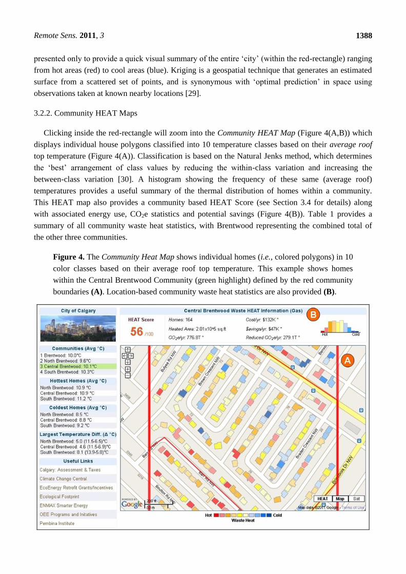
Clicking inside the red-rectangle will zoom into the Community HEAT Map (Figure 4(A,B)) which

displays individual house polygons classified into 10 temperature classes based on their average roof

top temperature (Figure 4(A)). Classification is based on the Natural Jenks method, which determines

the ‗best‘ arrangement of class values by reducing the within-class variation and increasing the

between-class variation [30]. A histogram showing the frequency of these same (average roof)

temperatures provides a useful summary of the thermal distribution of homes within a community.

This HEAT map also provides a community based HEAT Score (see Section 3.4 for details) along

with associated energy use, CO2e statistics and potential savings (Figure 4(B)). Table 1 provides a

summary of all community waste heat statistics, with Brentwood representing the combined total of

the other three communities.

Figure 4. The Community Heat Map shows individual homes (i.e., colored polygons) in 10

color classes based on their average roof top temperature. This example shows homes

within the Central Brentwood Community (green highlight) defined by the red community

boundaries (A). Location-based community waste heat statistics are also provided (B).


1389

Table 1. Summary of Community Waste Heat Statistics.

Community No of

Houses

Heated Area

(105 sq.ft)

CO2e

(T)

Reduced

CO2e (T)

Cost/yr

($103 CAD)

Savings/yr

($103 CAD)

Histogram

(house temp C

distribution)

Brentwood

(total of all

communities)

368 4.41 1704.1 620.6 288.6 105.1

North

Brentwood 95 1.17 452.1 199.5 76.6 33.8

Central

Brentwood 164 2.01 776.7 279.1 131.5 47.3

South

Brentwood 109 1.23 475.2 142.0 80.8 24.1

3.2.3. Home HEAT Maps

Clicking on a classified house polygon in the Community HEAT Map will display the

corresponding Home HEAT Map (Figure 5(A–G)). This map provides a detailed TABI waste heat

signature for a specific home, with roof temperatures automatically shown when moused over

(Figure 5(A)). In this example, the three hottest roof top locations (referred to as Hot Spots) are

automatically defined and represented as three colored circles (Figure 5(B)), with their accompanying

color-coded temperature values (Figure 5(C)). By clicking on the arrows [located at (Figure 5(C))] the

top 6 Hot Spots, their temperature values and locations will be cycled through, allowing the user to

visualize them within a house-context. In total, 6 interior, and 6 exterior (i.e., roof-edge) Hot Spots are

calculated for each home, but only the top three Hot Spots are shown at a time. This allows a home

owner to evaluate whether a Hot Spot represents the chimney, vent or some other roof object or area

of interest.

Our experience has shown that exterior roof Hot Spots typically correspond to heat escaping from

the doors and windows beneath them or from problem roof areas. These can be confirmed by clicking

on the Street View icon (Figure 5(D)). When, clicked, the residential heat map divides to allow the

corresponding Google Street View image to appear on its right hand side (Figure 5(E)). Users can then

zoom and pan around the Street View image which provides visual evidence of Hot Spot locations.

Alternatively, users can move their location in the residential heat map (Figure 5(F)), which

automatically updates their Street View perspective. In this example, a cursory visual comparison of

the Hot Spots (Figure 5(B)) and the Street View image (Figure 5(E)) reveals that waste heat is

escaping between the main home structure and the smaller front addition. To further evaluate this

scene, the user can also click on the ‗Sat‘ button (bottom middle of Figure 5) and view the house

polygons overlaid on the corresponding Google satellite or aerial imagery (not shown), rather than in

their current map view.


1390

Figure 5. The Home Heat Map provides a thermal image of an individual home showing:

(A) the moused-over roof temperature, (B) three Hot Spots and (C) their associated

temperatures, (D) the Google Street View icon linked to (E) the corresponding house

Street View. (F) shows the map location of the evaluated house. (G) defines the Fuel

Table, the associated fuel sources, the heating costs/day ($) and the resulting CO2e (kg).

Visual analysis of the Hot Spot locations (B) compared to the Street View image (E) reveal

that heat is escaping between the main home structure and the smaller addition

(front right).

3.2.4. The Fuel Table

In the Fuel Table (Figure 5(G)), the ($) cost per day of heating the home, along with estimated

CO2e (kg) for different geographically relevant fuel types (i.e., gas, oil, wind and hydro electricity,

etc.) are also modeled. These values are calculated based on (three years of) sample house data which

consists of the above-ground living area of the home, the natural gas (and electricity) used for space

heating per month, and the age and construction type of the home. Combined with Canmet Energy

models developed for the City of Calgary [31], these data are used to model the cost and quantity of

energy required for space heating all study site houses per day—weighted by their area and age (based

on City cadastral data). The Green House Gas emissions per day for CO2e are calculated based on this

home energy use model, and on CO2e coefficients provided from a recent Canadian energy mapping

study [1]. This study provides the CO2e coefficients generated for natural gas, and electricity from


1391

coal. In the absence of GHG coefficients for other fuel sources, the CO2e coefficient for oil is

calculated as a factor of the GHG coefficient of gas, and the CO2e coefficient of electricity from

renewable resources is calculated as a factor of the GHG coefficient of electricity from coal. In this

example (Figure 5(G)), electricity generated from coal is highlighted in green. When double clicked,

the view moves from the HEAT Score tab, to the $avings Tab, revealing the Annual Home Energy Use

Model (Figure 6(A–F)).

3.2.5. The Annual Home Energy Use Model

Based on sample house data (described in Section 3.2.4) and a specific local fuel type selected by

the user (Figure 6(A)), the Annual Home Energy Use Model provides a yearly estimate of the money

saved (Figure 6(B)) and the reduced CO2e (Figure 6(C)) if a home owner lowered their waste heat

(after correcting for the roof material emissivity—Section 2.2), from the maximum (Figure 6(D)), to

the minimum (Figure 6(E)) roof temperature (as defined for their house in the Home HEAT

Map—Figure 5). In this example (Electricity from Coal), it is estimated that a home owner could save

$522 and reduce their annual CO2e contribution by 10.2 tons, if they reduced their waste heat from

11.9 C to 8.8 C.

As previously indicated, all house temperature measurements above the ambient air temperature are

considered as waste heat. For this energy use model, the target waste heat temperature is not based on

reaching the ambient temperature, which would only be the case if the home had a perfectly insulated

living envelope and well performing attic ventilation (Section 4.6), or if the home‘s heating systems

were completely turned off for an extended period of time. Instead, our objective is to have users apply

energy efficiency enhancements (defined in the E-Tips tab—Figure 6(F)) to bring the maximum roof

top temperature, to the existing minimum temperature. Conceptually this is a reasonable expectation,

as the minimum roof temperature has already been reached at one or more roof locations (Figure

5(C)). Savings are calculated as the difference between the actual cost (assumed to be based on the

maximum roof top temperature) and the cost calculated as a function of the observed minimum roof

top temperature (Equation (2)).

Savings = Total Cost − (Total Cost ×

Minimum roof temperature/Maximum roof top temperature) (2)

Similarly, CO2e reductions are calculated as the difference between the emission, and the CO2e

emission calculated as a function of the minimum observed roof top temperature (Equation (3)).

CO2e Reductions = Total CO2e − (Total CO2e ×

Minimum roof temperature/Maximum roof top temperature) (3)

In the E-Tips tab (Figure 6(F)), energy efficiency information to assist in this goal will be provided

such as sealing obvious draught areas, improving living-envelop insulation, and improving the energy

efficiency of windows and doors, etc. More specialized information related to locally available HVAC

(Heating, Ventilating, and Air Conditioning) systems and service providers, alternative energy

sources—both off the grid (i.e., geothermal, wind, solar, tide, etc.)—and from (green) energy

providers, to NetZero construction [32] and LEED (Leadership in Energy and Environmental Design)

[33] certification for new and existing construction will also be provided.


1392

Figure 6. The $avings tab illustrates (A), the Annual Home Energy Use Model which

provides a yearly estimate of (B), the money saved and (C), the resulting CO2e reductions

if a home owner is able to reduce their waste heat from (D), the maximum to (E), the

minimum roof temperature based on energy efficiency information located in E-Tips (F).

3.3. Generating Hot Spots

The process of generating Hot Spot locations and statistics for individual houses begins with the

input of either thermal raster imagery alone, or both raster and vector data (Figure 7(1–6)). Thermal

imagery (Figure 7(1a)) is always required as an input, as it is the primary temperature source being

evaluated. The optional vector data represents building footprints (Figure 7(1b)), which if available, is

very useful. Without access to city cadastral polygons, GEOBIA feature extraction algorithms are used

to define individual house objects for the entire scene (Figure 7(2a)). In the case of both cadastral and

geobia objects (Figure 7(3)), or geobia objects only, a maximum of 12 Hot Spots are extracted—6

inside the roof envelope, and 6 along its 1 pixel wide perimeter—(Figure 7(5)), along with their related

geo-spatial statistics (Figure 7(6)). Conversely, with the use of cadastral house polygons, the Hot Spot

algorithms go through an iterative process (Figure 7(4)) of refining each GEOBIA object based on its

fit to its corresponding pre-existing house polygon, before identifying Hot Spots. This iterative

refinement procedure was initially created to ensure a strong visual agreement between GEOBIA and

cadastral house ‗objects‘ (typically > 80%) due to the high-order polynomial warping required during

geocorrection of the original TABI-320 image (Section 2).


1393

Figure 7. The Hot Spot processing flow-diagram, showing paths for both raster and vector data.

When large discrepancies are detected between the geobia defined houses and the cadastral houses

the resulting objects are flagged for further investigation and manual verification by an analyst. Along

with this flag, many other statistics are calculated for all geobia houses, which may further be used in

KDD (Knowledge Discovery from Databases) and data mining [34]. Figure 8(A) illustrates a 79.4%

agreement between the GEOBIA roof object (center green) derived from the TIR image, and the

corresponding City polygon (center red) derived from a manually digitized color aerial

ortho-photo-mosaic. Figure 8(B) shows the Hot Spots (red dots) constrained within the GEOBIA

object boundaries, and (Figure 8(C)) shows three corresponding circular Hot Spots located on a

colorized waste heat image (blue is cold, red is hot). The minimum distance between Hot Spot

locations is pre-defined by an analyst (i.e., 2–4 pixels apart), so that a clustering effect does not

visually occur in the image; which due to the limited number of Hot Spots able to be shown at a single

time (i.e., 3 out of 6), could result in other more spatially distributed (and useful) Hot Spot locations

being missed.

Figure 8. An example of (A) the fit between geobia (green) and cadastral (red) house

objects, (B) their associated Hot Spots (red dots), and (C) how these Hot Spots appear on

the thermal image. Hot Spot are thermally ranked from hottest to coldest (red, orange,

yellow), and displayed three at a time (see Figure 5(B)).


1394

3.4. The HEAT Score Algorithm

Numeracy—the ability to reason with numbers and other mathematical concepts—is applied in

decision support and risk analysis assessments, where either hard, or easy to evaluate attributes are

provided to users, to examine their influence on user preferences [35]. The rule of thumb from

numerous studies is essentially, ‗…that numbers matter…‘ and that when given a choice, ―…subjects

typically prefer larger numbers, than smaller numbers...‖ (see Section 4.5 for details). In a related

Geoweb example, the Walk Score website (www.walkscore.com/) provides a walk ability measure for

‗any‘ North American home address based on a number of estimated factors, such as distance to

schools, shopping, healthcare, etc. Results show that this single Walk Score value (defined out of 100)

also has important implications for the real-estate market, where one point of Walk Score is worth up

to $3,000 of property value to that home [36].

In order to meaningfully compare the waste heat of one or more houses with all other houses in the

city, we have developed a normalized HEAT Score based on the z-score or standardized score [37]. A

standard score indicates how many standard deviations an observed value, (in this case the average

roof top temperature), is above or below the population mean. For our HEAT Score, this represents the

average of all the average roof top temperatures in the city. Similarly, our population represents all the

houses in the city, or more specifically all the houses in the Brentwood community dataset. Based on

the standard score formula (Equation (4)) the HEAT Score is calculated as shown in Equations (5)

and (6):

[z-score = (x − μ)/σ] (4)

x is the average roof top temperature to be standardized, μ is the average of all the average roof top

temperatures in the city, and σ is the standard deviation of the average roof top temperatures in the

city. Z-scores follow a standard normal distribution; consequently 99.98 percent of the values will lie

between −3.49 and 3.49. In our case, this z-score is proportionately converted to a scale from 0 to 100,

to represents the HEAT Score for every home.

HEAT Score = (z-score of an item − (−3.5))/(3.5 − (−3.5) × 100) (5)

HEAT Score = (z-score + 3.5)/7 × 100 (6)

In Equations (5) and (6), the value of 3.5 is used instead of 3.49 to provide a buffer so that we can

include 0.02% (100–99.98) of the values which might occur in this distribution. By using this HEAT

score an individual can compare their house, with any other house in any part of the city. In simple

terms, if the HEAT Score for a home is 91% it would indicate that ―…this home wastes more HEAT

than 91% of the other homes in this city‖. Associated with each HEAT Score would also be a relative

descriptor, which for 91% would state ―…Very High Waste HEAT…‖ Additional examples are shown

in Table 2. The City HEAT Score is calculated based on the average HEAT Score of all houses in the

City (see Figure 3), while the Community HEAT Scores are calculated based on the average HEAT

Score for all the houses in each community (see Figure 4).


1395

Table 2. HEAT Score ranges and relative descriptors.

Heat Score Relative Descriptor

90–100 Very high

75–89 High

50–74 Moderately High

25–49 Moderately Low

10–24 Low

0–9 Very Low

4. Discussion—Challenges, Lessons, Solutions

In this section we discuss critical challenges we still face, lessons learned, and briefly describe

proposed solutions that we are currently working on for Phase II of the HEAT project, as we scale

from 368 to 300,000+ homes and begin using TABI-1800 data. Specifically we will: (i) discuss

Phase I limitations with the TABI-320 for large urban areas, and propose a TABI-1800 solution; (ii)

introduce a new Object-Based Mosaic algorithm that solves the problem of bifurcated roof/house

objects along the mosaic seam; (iii) propose Emissivity Modulation to convert the image to true

temperatures; (iv) introduce Thermal Urban Road Normalization (TURN), a new object-based method

to correct for local climatic variability during data acquisition; (v) discuss concerns with the HEAT

Scores and describe how to implement a Carbon Score; and (vi) provide an example where errors in

the City‘s cadastral database could be corrected from a combination of GEOBIA (feature detection)

and TABI data.

4.1. TABI Acquisition Limitations and Solutions

The small footprint of the TABI-320 makes it well suited for narrow-width long-transect data

acquisitions such as along transmission- and pipe-lines, but impractical for acquiring large area urban

datasets. For example, to image the entire city of Calgary (24 × 35 km) 160 flight lines would need to

be collected over 15 days at a cost of $150K+ (CAD: based on a 2009 ITRES acquisition quote).

Additionally, serious thermal calibration problems would undoubtedly arise due to weather differences

over such a long acquisition time (see Haringey TIR acquisition in Section 1). To overcome these

challenges, we suggest that the solution for future large-area high-resolution urban thermography data

acquisitions will be found with the new TABI-1800 [38].

The TABI-1800 has a swath width of 1,800 pixels, and ability to collect up to 175 km2 per hour at

1.0 m spatial resolution. This is three to five times larger and faster than most other airborne TIR

sensors. The TABI-1800 calculates radiometrically calibrated and geo-referenced data when in the air

and uses diffraction-limited optics to ensure spatial independence of each pixel to avoid smearing

between pixels. The Stirling Cycle cooled MCT (mercury cadmium telluride) detectors are four times

faster than the non-cooled ones used in most TIR sensors, thus allowing for the rapid detection of

much weaker thermal signals (i.e., thermal resolution 0.05 C), while diminishing thermal drift as

compared to bolometer-based systems [38]. We note that on 31 March 2011 (between 24:00 and 4:45

hrs MST), twenty three 35 km long flight lines were acquired by the TABI-1800 over the City of


1396

Calgary Alberta in its maiden acquisition. The resulting dataset were acquired at a 70 cm spatial

resolution in just over 4.5 hrs total flight time on a single fuel tank (Navajo platform), at about ¼ the

cost of the TABI-320. No other TIR system currently exists like this anywhere in the world. Lessons

learned from working with the TABI-320 in Phase I of the HEAT project will be applied to this new

dataset in Phase II, to create evidence based geoinformation to facilitate enhanced energy efficiency

decisions for some 300,000+ Calgary homes, with plans to apply worldwide.

4.2. Object-Based Mosaicing (OBM)

The TABI-320 scene is composed of two flight lines that are mosaiced with a 30% overlap between

each flight line [39]. Due to geometric and radiometric variations (in this case primarily from

microclimatic thermal variability) during different acquisition times, similar objects may have

different spectral characteristics within and between flight lines [40]. In the TABI-320 dataset, this

temporal difference is most apparent where the mosaic seam divides one or more house objects,

resulting in different temperatures for each portion of the affected house; which in turn incorrectly

biases temperature based statistics (Table 2). In the recently collected TABI-1800 dataset there are 23

flight lines, (each 35 km long), sampling a city of 300K+ homes. Thus, potential exists for many

thousands of roof objects to be affected, and incorrectly assessed. To mitigate this condition, we

propose a new GEOBIA method referred to as Object-Based Mosaicing (OBM) (Figure 9) and

describe the pseudo code to incorporate only whole roofs within the mosaic process. In all cases we

assume that each flight line has previously been geometrically corrected by the data provider with a

spatial error of ±2 pixels (or less).

4.2.1. OBM Pseudo Code

In the case where cadastral polygons exist, each flight needs to be geometrically corrected to the

corresponding roof-top polygons.

In the case where only thermal data exists, object-based feature detection will be applied to each

flight line (separately) to extract roof-top polygons.

A suitable sized buffer around each roof [e.g., 2–3 times the reported geometric correction error (in

pixels)] needs to be generated to compensate for unresolved local geometric errors between

flight lines.

For two adjacent flight lines, the overlap between each flight line will be defined, from which a

linear center mosaic line will be defined (yellow line in Figure 9).

The buffered roofs that are divided by the flight line will be identified.

Based on the proximity of each bifurcated roof to the center of its flight line (so as to reduce radial

displacement effects) the center mosaic line will be joined around defined roof buffers (red line

Figure 9), and used to mosaic adjacent datasets together.

This process is then applied to the next adjacent flight line and repeated until all flight lines

are mosaiced.


1397

Figure 9. A graphic of two flight lines (pink and blue), with a 30% overlap (purple) are

shown along with an example of the resulting object-based mosaic line (red) derived from

a joining of the initial mosaic line (yellow) and the buffered (blue) roof-top objects (grey).

4.3. Emissivity Modulation (EM)—Correcting for Emissivity

Defining Hot Spots does not require the TABI data to be converted to true temperatures, because

we search only within a single roof object, and we assume that based on its 1.0 m spatial resolution in

comparison to the (much smaller) sized objects typically found on a roof (e.g., vents), that the roof

material is essentially homogenous. Thus any difference in roof temperature is due to thermal

conductance from the (lower) living envelope. However, if the spatial resolution of the TABI data

were closer to 0.25 m then individual pixels would be more representative of (plastic and metal) vents

and other objects found on the roof; which would require solving the emissivity for each material type.

In the Phase I situation, spatial scale (considered as pixel size) reduces the thermal complexity of roof

materials. However, if we develop energy models based on differences between the maximum and

minimum roof temperatures for each roof, and we compare those results with different roofs to create a

HEAT Score, then we need to first correct for different roof materials.


1398

Early attempts have been made to quantify the impact of emissivity on estimating the true kinetic

temperature from remote sensing imagery. The simplest method used by researchers was to integrate

the thermal data with the corresponding land use data [41,42]. Similarly, Savelvev and Sugumaran

[43] collected ground truth data (i.e., radiant temperature) of objects with known emissivity, which

were then integrated with Planck‘s Law [44] to develop an empirical regression model for calculating

the true kinetic temperature of image pixels. Recently, the Emissivity Modulation technique [45] was

proposed to perform spatial enhancement and emissivity correction of ASTER (90 m) thermal bands

using a higher resolution optical image (ASTER 15 m). For this study, we propose to apply the

Emissivity Modulation technique to the 1.0 m TABI-320 using a 1.0 m RGB airphoto (resampled from

our existing 30 cm RGB airphoto). To the best of our knowledge this has never been applied to such

an H-res dataset. This method is expected to increase accuracy in the computation of kinetic

temperature, improve the relationship between image values and air temperature, and better enable the

observation of microscale temperature patterns [45]. If successful, we will also apply this procedure to

the new TABI-1800 dataset.

4.4. Thermal Urban Road Normalization (TURN)—Correcting for Local Climatic Variability

Thermal remote sensing is strongly influenced by local microclimatic variability [46] of which the

main components are wind, precipitation, and humidity. (i) Surface winds increase convective heat

loss from ground objects and make them cooler [47]. (ii) Precipitation forces objects to cool down and

to achieve a uniform temperature state [48], and (iii) as the humidity increases, ground targets appear

to be cooler [46]. Thus, objects of similar thermal state but placed in varied microclimatic conditions

will exhibit different temperature measurements from thermal remote sensors.

The importance of modeling local climatic variability to reveal surface temperature is described by

Voogt and Oke [5] and others [46,49]. However, to the best of our knowledge, we have found no urban

thermal study that considers the influence of local climatic variability on remote sensor observation.

This may be explained because local climate variables differ dramatically within very small

spatio-temporal scales. Consequently, it is difficult to develop models to predict such variations.

Additionally, in the past the availability of high-resolution TIR data for large urban areas has been

limited [50]. In the case of airborne TIR imagery, the ambient sensed temperature also naturally

changes during, and between flight line acquisitions, resulting in mosaiced images with different

temperatures for the same (overlapping) scene components, making detailed analysis non-trivial (see

Section 4.2).

In an effort to minimize the effects of local microclimatic variability from different flight paths, we

briefly introduce the Thermal Urban Road Normalization (TURN) algorithm, which is based on the

idea of pseudo invariant features, such as roads or highways (i.e., concrete, gravel, tar) which during

TIR acquisition are expected to be at a constant scene temperature (see roads in Figure 1). Thus, any

variation observed in (average) road temperature throughout the scene is assumed to be the effect of

local climate variation; which we suggest is a valid assumption for acquisitions late at night, or early in

the morning in northern winter climates. Essentially the TURN model will calculate deviations from

average road temperatures and will then adjust the temperature of the entire image, based on an

interpolation of mean-deviation temperatures between roads.


1399

4.4.1 TURN Pseudo Code

The pseudo code for creating TURN is described as follows:

Begin by isolating roads of a common material type either from an available GIS road layer, or

using GEOBIA methods to segment and define specific road types in the TIR image.

A 1.5 m buffer will then be created around each side of the road center (thus 3.0 m total diameter)

to remove sidewalks, parked vehicles, curb side drains etc., or in the case of segmented roads, the

mathematical morphology function erosion can be applied until a 3.0 m road skeleton remains.

The remaining road object will then be emissivity corrected for material types (i.e., concrete,

gravel, tar) to generate a ‗kinetic‘ or ‗true‘ temperature ‗road‘ object.

A random sample will extract 20% of these ‗true‘ road pixels for an accuracy assessment, while the

mean of the remaining (80%) road pixels will be calculated.

The mean temperature deviation per unit temperature for each ‗true-road‘ pixel will then

be calculated.

The mean deviation will be interpolated over the entire image using three different interpolation

methods: (i) Ordinary Kriging; (ii) Inverse Distance Weighting; and (ii) Splines.

The temperature of all scene pixels will then be adjusted with the mean deviation values.

An accuracy assessment will be performed for the three interpolation methods separately using the

extracted (20%) road pixels. It is expected that the model will generate average road temperatures

for each road pixel. Any deviation from the average temperature will be considered as an error

(due to microclimatic variation).

The RMSE will then be calculated for each interpolation method, and their accuracies will

be compared.

The resulting normalized image with the lowest RMSE and most visually meaningful results will

then be used for further analysis.

4.5 HEAT and Carbon Scores

A concern with the current HEAT Score is that intuitively, higher scores are generally considered

‗better‘ than lower scores (Section 3.4). In its current state, the higher the HEAT Score, the greater the

waste heat generated by the home. However, we do not want to ‗celebrate‘, ‗support‘ or ‗promote‘

high waste heat, but rather the opposite. Unfortunately, a simple reversal of the algorithm, where a low

wasteheat score represents a high HEAT Score, does not make sense. Furthermore, as currently

calculated, the HEAT score cannot be used to compare houses in different cities. In order to allow for

intra-city waste heat competitions, this will need to be solved, but as we currently do not have

additional data, this is relegated to future work. In the meantime we are currently developing a

‗Carbon Score‘. This is based on the Fuel Table (Section 3.2.4) calculations for each home, which are

weighted by livable house area, and the estimated CO2e (kg) from the fuel type used [1,31]. Similar to

the existing Community and City HEAT maps, we will also generate classified Carbon Maps to

spatially model ‗carbon‘ distribution associated with home/community/city energy usage.


1400

4.6. Updating Cadastral Errors with GEOBIA and Thermal Imagery

The automated GEOBIA approach to house extraction from the TABI-320 data has shown

unexpected positive results by automatically ‗flagging‘ houses with house boundary digitizing errors

from the city cadastral vector dataset (on the order of 6%). If this error relationship holds valid for the

entire 300,000+ homes located in Calgary, this represents a potential of some 18,000+ home

boundaries incorrectly recorded within the official cadastral record. The probability that the same kind

of errors exist in other cities is also high. Thus, potential exists for this thermal-based house boundary

information to be provided as a commercial product to interested municipalities. At present this

relationship has not been verified over a larger sample, however, our intention is to further examine

this in the TABI-1800 scene, and to evaluate interest from the city for related geoinformation products.

In the Brentwood dataset, these 6% digitizing errors have been verified using the HEAT Google Street

View functionality (see Figure 5) which allows for individual homes to be viewed from multiple

angles, not just from a plan-view as in the Google satellite or aerial photography. For example, in

Figure 10 a thermal sub-image (Figure 10(A)) reveals that a house and garage (in blue and green) are

two separate entities, adjacent to a central ‗hot‘ area (in red). In (Figure 10(B)) the cadastral house

polygon defines both of these structures as a single house vector. Since the cadastral polygon is larger

than the average size of the neighboring polygons, and does not perfectly agree with the area of the

GEOBIA house object, it was automatically flagged for further visual analysis (see Section 3.3).

(Figure 10(C)) Shows a corresponding 30 cm air photograph sub-image of the scene which visually

appears to correlate with the cadastral polygon (Figure 10(B)); however a Google Street View

perspective of this garage and house combination (Figure 10(D)), reveals that this manually drawn

cadastral polygon is incorrect (as it failed to distinguish the temporary roof), but that the separate

thermal house and garage structures (Figure 10(A)) are indeed correct.

5. Conclusion

With the primary goal to improve urban energy efficiency by developing geospatial technologies

that provide effective user feedback, the HEAT pilot project is a FREE Geoweb mapping service

designed to allow residents to visualize the amount, location and cost of waste heat leaving their

homes and communities as easily as clicking on their house in Google Maps. HEAT incorporates

geospatial solutions for residential waste heat monitoring using Geographic Object-Based Image

Analysis (GEOBIA) and Canadian built Thermal Broadband Airborne Imager (TABI) technology to

provide users with timely, in-depth, easy to use, location-specific waste-heat information; as well as

opportunities to save their money and reduce their green house gas emissions. In this paper, we

describe the HEAT Phase I pilot project which evaluates 368 residences in the Brentwood community

of Calgary, Alberta, Canada. This FREE service: (i) defines the 6+ hottest locations on each home, and

relates them to windows, doors, roofing, and/or insulation solutions from local service providers; (ii)

automatically links each home to Google Street View to confirm Hot Spot locations; (iii) provides

green house gas and space-heating estimates for different fuel types for each home; (iv) identifies the

hottest homes in each community; and (v) provides a HEAT Score for comparative analysis and

monitoring at the house, community and city scales. We also discuss lessons learned from Phase I as

we prepare to scale to 300,000+ homes (in Phase II) with the newly developed TABI-1800.


1401

Specifically, we introduce a new object-based mosaicing strategy, an adaptation of Emissivity

Modulation to correct for emissivity differences, a new Thermal Urban Road Normalization (TURN)

technique to correct for scene-wide microclimatic variation, and describe a new Carbon Score. We

also show that a combination and TABI and GEOBIA feature detection could be used to update (a

possible 18,000+) incorrect house polygons that potentially exist within the City Cadastral dataset.

Figure 10. A house and garage are shown as two separate entities in a TABI-320

sub-image (1.0 m) (A), while the cadastral house polygon (B) defines them as a single

house vector. (C) shows a corresponding air photograph (30 cm) of the scene which

visually correlates with the cadastral polygon; however a Google Street View perspective

(D), reveals that this cadastral polygon is incorrectly drawn, and that the thermal

information is correct.


1402

Since these free energy-efficiency decision support tools provide information at the house,

community and city scale, they may also: (i) provide service agencies evidence of successfully

implementing energy retrofit programs; and (ii) opportunities to promote national and international

intra- and inter-city waste heat competitions. Additionally (iii) renovation contractors may find these

tools useful for identifying neighborhoods for marketing energy efficiency upgrades, or (iv) residential

service providers offering energy efficiency solutions. (v) Construction companies could also use these

results to verify the energy-efficiency quality of their homes, and (iv) real estate agents, could use

them to assist energy conscious clients. Law enforcement agencies may also be able to (v) use this

spatial intelligence for identifying energy theft, and (vi) illegal grow-ops. Additional uses may be

found by (vii) municipal planners looking to identify the ‗best‘ communities to focus energy efficiency

incentives upon, and (viii) to support Government and municipal Energy Efficiency and Ecological

Footprint programs.

HEATs mission is to show what urban energy efficiency looks like, where it is located, what it

costs, and what to do about it. We believe that if people could see the waste heat they generate and if

they knew how much it cost (from a $$ and environmental perspective), that they would want to take

action. We want to show them how. Ultimately, our vision is to empower the urban energy efficiency

movement by providing free, accurate and regularly updated TIR waste heat solutions for the world.

To evaluate the current version of HEAT, please login to (http://www.wasteheat.ca) as beta, with the

password beta (no italics).

Acknowledgements

Geoffrey Hay acknowledges critical support from The Institute for Sustainable Energy,

Environment and Economy (www.iseee.ca), ITRES Research Limited (www.itres.com), the City of

Calgary (www.calgary.ca), the Urban Alliance (www.urban-alliance.ca), the UofC Foothills Facility

for Remote Sensing and GIScience (www.ucalgary.ca/f3gisci), the University of Calgary–ARTS

Information Technologies Team (http://arts.ucalgary.ca/it/), The Tecterra GECKO program

(www.tecterra.com) and NSERC (www.nserc.ca). We also acknowledge an Alberta Informatics Circle

of Research Excellence (iCore) PhD Scholarship awarded to Gang Chen, and a University of Calgary

Faculty Graduate Research Scholarship and a Geography Excellence Award provided to Mir

Mustafizur Rahman. We also thank Ryan Powers for his early HEAT research contributions. The

opinions expressed here are those of the authors, and may not reflect the views of their funding

agencies.

References

1. CUI. Energy Mapping Study; Canadian Urban Institute: Toronto, ON, Canada, 19 December

2008; p. 92. Available online: http://www.calgary.ca/docgallery/BU/planning/pdf/plan_it/

energy_mapping_study.pdf (accessed on 1 April 2011).

2. Darby, S. The Effectiveness of Feedback on Energy Consumption; Report published by

Environmental Change Institute; University of Oxford: Oxford, UK, 2006. Available online:

http://www.eci.ox.ac.uk/research/energy/downloads/smart-metering-report.pdf (accessed on 1

April 2011).


1403

3. Marsden, G. Beyond Your Utility Meter: Three Energy Monitors for Your Toolbox. Home Power

August/September 2010, 138, 54-58.

4. Google. A Letter to the President of the United States; 2010. Available online:

https://sites.google.com/site/obamaenergyletter/home/ (accessed on 5 July 2011).

5. Voogt, J.A.; Oke, T.R. Thermal remote sensing of urban climates. Remote Sens. Environ. 2003,

86, 370-384.

6. Allinson, D. Evaluation of Aerial Thermography to Discriminate Loft Insulation in Residential

Housing. Ph.D. Thesis, University of Nottingham, Nottingham, UK, 2007. Available online:

http://etheses.nottingham.ac.uk/284/ (accessed on 1 April 2011).

7. Weng, Q. Thermal infrared remote sensing for urban climate and environmental studies: Methods,

applications, and trends. ISPRS J. Photogramm. Remote Sens. 2009, 64, 335-344.

8. Stockton, G.R. Aerial infrared Thermagraphy. Cadalyst September 2004, 21, 47-53.

9. Jensen, J.R. Thermal Infrared Remote Sensing. In Remote Sensing of the Environment: An Earth

Resource Perspective; Chapter 8; Prentice Hall: Upper Saddle River, NJ, USA, 2007; pp. 249-290.

10. Frost & Sullivan. US Commercial and Military Infrared Imaging System Markets; Report

A020-Pub.8; 2001.

11. Hay, G.J.; Hemachandran, B.; Kyle, C.D. HEAT (Home Energy Assessment Technologies):

Residential waste heat monitoring, Google Maps and airborne thermal imagery. GIM Int. 2010, 3,

13-15.

12. Council Claims Back Cash after ‘Heat Map’ Fails; 13 May 2010. Available online:

http://www.portsmouth.co.uk/news/local/east-hampshire/council_claims_back_cash_after_heat_

map_fails_1_1251057 (accessed on 30 January 2011).

13. Clark, M.L; Aide, T.M. Virtual Interpretation of Earth Web-Interface Tool (VIEW-IT) for

Collecting Land-Use/Land-Cover Reference Data. Remote Sens. 2011, 3, 601-620.

14. Geoweb. Available online: http://www.Geowebconference.org/ (accessed on 1 April 2011).

15. Digital Earth. Available online: http://en.wikipedia.org/wiki/Digital_Earth (accessed on 1 April

2011).

16. Pyxisinnovation. Available online: http://www.pyxisinnovation.com/ (accessed on 1 April 2011).

17. Hay, G.J.; Blaschke, T. Forward: Special Issue on Geographic Object-Based Image Analysis

(GEOBIA). Photogramm. Eng. Remote Sensing 2010, 76, 121-122.

18. Ushahidi. Available online: http://vimeo.com/ushahidi (accessed on 1 April 2011).

19. Firemap. Available online: http://firefly.geog.umd.edu/firemap/ (accessed on 1 April 2011).

20. Hay, G.J.; G. Castilla. Geographic Object-Based Image Analysis (GEOBIA): A new name for a

new discipline? In Object-Based Image Analysis: Spatial Concepts For Knowledge-Driven Remote

Sensing Applications; Blaschke, T., Lang, S., Hay, G.J., Eds; Chapter 1.4; Springer-Verlag: Berlin,

Germany, 2008; pp. 75-89.

21. TABI-320. Available online: http://www.itres.com/products/imagers/tabi320 (accessed on 1 April

2011).

22. Jacob, F.; Francois, P.; Schmugge, T.; Vermote, E.; French, A.; Ogawa, K. Comparison of Land

Surface Emissivity and Radiomatric Temperature Derived from MODIS and ASTER. Remote

Sens. Environ. 2004, 90, 137-152.


1404

23. Parker, D.S.; McIlvaine, J.E.R.; Barkaszi, S.F.; Beal, D.J.; Anello, M.T. Laboratory Testing of the

Reflectance Properties of Roofing Material; FSEC-CR-670-00; Florida Solar Energy Center:

Cocoa, FL, USA, 2000.

24. Steiniger, S.; Hay, G.J. Free and Open Source Geographic Information Tools for Landscape

Ecology: A Review. Ecol. Inf. 2009, 4, 183-195.

25. GNU Data Language. Available online: http://gnudatalanguage.sourceforge.net/ (accessed on 21

June 2011).

26. Segmentation Evaluation. Available online: http://www.ioer.de/segmentation-evaluation/

index.html (accessed on 21 June2011).

27. Neubert, M.; Herold, H.; Meinel, G. Assessing image segmentation quality—Concepts, methods

and application. In Object-Based Image Analysis: Spatial Concepts for Knowledge-Driven

Remote Sensing Applications; Blaschke, T., Hay, G., Lang, S., Eds.; Lecture Notes in

Geoinformation & Cartography; Springer: Berlin, Germany, 2008; pp. 769-784.

28. Allen, T.F.H.; Starr, T.B. Hierarchy Perspective for Ecological Complexity; University of

Chicago Press: Chicago, IL, USA, 1982; p. 310.

29. Cressie, N. The Origins of Kriging. Math. Geology 1990, 22, 239-252.

30. Jenks, G.F. The Data Model Concept in Statistical Mapping. Int. Yearbook Cartogr. 1967, 7,

186-190.

31. The Urban Archetypes Project. Community Case Study: The City of Calgary; Canmet ENERGY

Cat. No. M154-15/3-2009 E-PDF; CanmetENERGY: Ottawa, ON, Canada, 2009; p 10. Available

online: http://canmetenergy-canmetenergie.nrcan-rncan.gc.ca/eng/publications.html?Cat.%20

No.%20M154-15/3-2009E-PDF%20%28On-line%29%20%20%20ISBN%20978-1-100-11950-2

(accessed on 1 April 2011).

32. NetZero Buildings. Available online: http://en.wikipedia.org/wiki/Zero-energy_building

(accessed on 1 April 2011).

33. LEED. Available online: http://en.wikipedia.org/wiki/Leadership_in_Energy_and_

Environmental_Design (accessed on 1 April 2011).

34. Piatetsky-Shapiro, G. Knowledge Discovery in Real Databases: A Report on the IJCAI-89

Workshop. AI Magazine 1991, 11, 68-70.

35. Wilson, R.S.; Arvai, J.L. When Less is More: How Affect Influences Preferences When

Comparing Low and High-risk Options. J. Risk Res. 2006, 9, 165-178.

36. Walkscore value. Available online: http://blog.walkscore.com/2009/08/new-study-shows-one-

point-of-walk-score-worth-up-to-3000/ (accessed on 31 March 2011).

37. Z-score. Available online: http://en.wikipedia.org/wiki/Standard_score (accessed on 1 April 2011).

38. TABI-1800 Product Information. Available online: http://www.itres.com/products/imagers/

tabi1800/ (accessed on 1 April 2011).

39. Afek, Y.; Brand, A. Mosaicking of Orthorectified Aerial Images. Photogramm. Eng. Remote

Sensing 1998, 64, 115-125.

40. Tuominen, S.; Pekkarinen, A. Local radiometric correction of digital aerial photographs for multi

source forest inventory. Remote Sens. Environ. 2004, 89, 78-82.


1405

41. Balling, R.C.; Brazell, S.W. High Resolution Surface Temperature Patterns in a Complex Urban

Terrain. Photogramm. Eng. Remote Sensing 1988, 54, 1289-1293.

42. Weng, Q. A Remote Sensing-Gis Evaluation of Urban Expansion and Its Impact on Surface

Temperature in the Zhujiang Delta, China. Int. J. Remote Sens. 2001, 22, 1999-2014.

43. Savelyev, A.; Sugumaran, R. Surface Temperature Mapping of the University of Northern Iowa

Campus Using High Resolution Thermal Infrared Aerial Imageries. Sensors 2008, 8, 5055-5068.

44. Rybicki, G.B.; Lightman, A.P. Radiative Process in Astrophysics; John Wiley and Sons: New

York, NY, USA, 1979.

45. Nicole, J.E. An Emissivity Modulation Method for Spatial Enhancement of Thermal Satellite

Images in Urban Heat Island Analysis. Photgramm. Eng. Remote Sensing 2009, 75, 1-10.

46. Hartz, D.A.; Prashad, L.; Golden, J.; Brazel, A.J. Linking Satellite Images and Hand Held Infrared

Thermography to Observe Neighborhood Climate Conditions. Remote Sens. Environ. 2006, 104,

190-200.

47. Santamouris, M.; Papanikolaou, N.; Livada, I.; Koronakis, I.; Georgakis, A.; Assimakopoulos,

D.N. On the Impact of Urban Climate on the Energy Consumption of Buildings. Solar Energy

2001, 70, 201-216.

48. Giannini, A.; Saravanan, R.; Chang, P. Oceanic Forcing on Sahel Rainfall on Interannual to

Interdecade Time Scales. Science 2003, 302, 1027-1030.

49. Weng, Q.; Lu, D. A Sub-Pixel Analysis of Urbanization Effect on Land Surface Temperature and

Its Interplay with Impervious Surface and Vegetation Coverage in Indianapolis, United States.

Int. J. Appl. Earth Obs. Geoinf. 2008, 10, 68-83.

50. Pu, R.; Gong, P.; Michishita, R.; Sasagawa, T. Assessment of Multi-Resolution and Multi-Sensor

Data for Urban Surface Temperature Retrieval. Remote Sens. Environ. 2006, 104, 211-225.

© 2011 by the authors; licensee MDPI, Basel, Switzerland. This article is an open access article

distributed under the terms and conditions of the Creative Commons Attribution license

(http://creativecommons.org/licenses/by/3.0/).

geospatial technologies to improve urban energy …...geospatial technologies to improve urban...

Documents