geos: geodesic image segmentation - microsoft.com geodesic image segmentation antonio criminisi,...

GeoS: Geodesic Image Segmentation

Antonio Criminisi, Toby Sharp, and Andrew Blake

Microsoft Research, Cambridge, UK

Abstract. This paper presents GeoS, a new algorithm for the efficientsegmentation of n-dimensional image and video data.

The segmentation problem is cast as approximate energy minimiza-tion in a conditional random field. A new, parallel filtering operatorbuilt upon efficient geodesic distance computation is used to propose aset of spatially smooth, contrast-sensitive segmentation hypotheses. Aneconomical search algorithm finds the solution with minimum energywithin a sensible and highly restricted subset of all possible labellings.

Advantages include: i) computational efficiency with high segmentationaccuracy; ii) the ability to estimate an approximation to the posterior oversegmentations; iii) the ability to handle generally complex energy models.Comparison with max-flow indicates up to 60 times greater computationalefficiency as well as greater memory efficiency.

GeoS is validated quantitatively and qualitatively by thorough com-parative experiments on existing and novel ground-truth data. Numerousresults on interactive and automatic segmentation of photographs, videoand volumetric medical image data are presented.

1 Introduction

The problem of image and video segmentation has received tremendous attentionthroughout the history of computer vision with excellent recent results beingachieved both interactively [1,2] and automatically [3]. However, state of the arttechniques are not fast enough for real-time processing of high resolution images(e.g. > 2Mpix). This paper describes a new, efficient algorithm for the accuratesegmentation of n-dimensional, high-resolution images and videos.

Like many vision tasks, the segmentation problem is usually cast as energyminimization in a Conditional Random Field (CRF) [1,2,4,6,7]. This encouragesspatial-smoothness and contrast-sensitivity of the final segmentation. The sameframework is employed here; but in contrast to graph cut-based approaches herethe segmentation is obtained as the labeling corresponding to the energy min-imum (MAP solution) found within a restricted, sensible subset of all possiblesegmentations. Such a solution will be shown to be smooth and edge aligned. Thesegmentation posterior over the selected subspace can also be estimated, thusenabling principled uncertainty analysis (see also [5]). Quantitative comparisonswith ground truth will demonstrate segmentation accuracy equal or superior

D. Forsyth, P. Torr, and A. Zisserman (Eds.): ECCV 2008, Part I, LNCS 5302, pp. 99–112, 2008.c© Springer-Verlag Berlin Heidelberg 2008

100 A. Criminisi, T. Sharp, and A. Blake

to that of the global minimum as found by min-cut/max-flow1. Restricting thesearch space to a small, sensible one accounts for the computational efficiency.

Similar to the work of Bai et al. in [9], we also use geodesic transforms toencourage spatial regularization and contrast-sensitivity. However, GeoS differsfrom [9] in a number of ways: i) The technique in [9] assumes given user strokesand imposes an implicit connectivity prior which forces each region to be con-nected to one such stroke2. In contrast, our geodesic filter acts on the energyunaries (not the user strokes). This allows GeoS to generate segmentations withno topological restrictions. ii) GeoS is not specific to interactive segmentationand can be applied to automatic segmentation as well as other tasks such asdenoising, stereo and panoramic stitching. iii) GeoS presents a clear energy tobe minimized. This allows quantitative comparisons with other energy-basedapproaches such as GrabCut [2]. Finally, iv) Despite the complexity of bothalgorithms being optimally linear in the number of pixels, GeoS, thanks to itscontiguous memory access and parallelism is much faster than [9] in practice.

Efficient segmentation via energy minimization has also been the focus of thedual-primal technique in [10] and the logarithmic α-expansion scheme in [11]. Inspatio-temporal MRFs efficiency may be gained by either reusing the graph flowor the search trees [12,13]. Instead, the efficiency of GeoS stems from its opti-mized memory access and its ability to exploit the power of modern multi-corearchitectures. In contrast, graph-cut does not lend itself to easy parallelization.

Finally, unlike graph-cut, our approximate minimization algorithm is not re-stricted to a specific family of energies. This enables us to experiment with moresophisticated models, like those containing global constraints.

2 Background on Distance Transforms

This section presents background on geodesic distances and related algorithms.

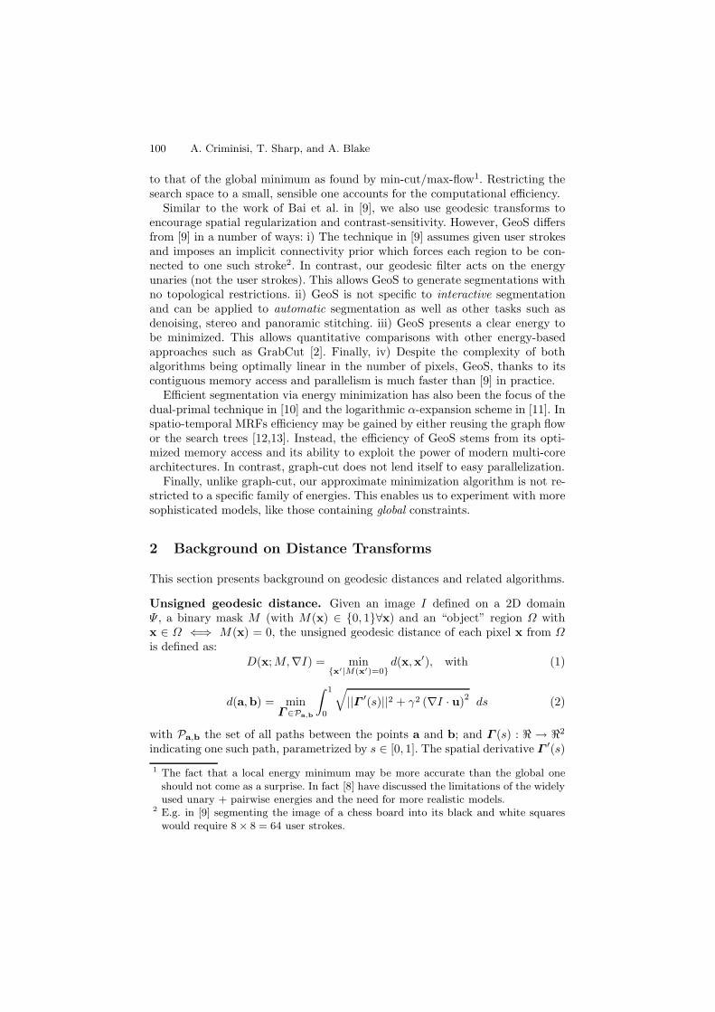
Unsigned geodesic distance. Given an image I defined on a 2D domainΨ , a binary mask M (with M(x) ∈ {0, 1}∀x) and an “object” region Ω withx ∈ Ω ⇐⇒ M(x) = 0, the unsigned geodesic distance of each pixel x from Ωis defined as:

D(x; M,∇I) = min{x′|M(x′)=0}

d(x,x′), with (1)

d(a,b) = minΓ ∈Pa,b

∫ 1

0

√||Γ ′(s)||2 + γ2 (∇I · u)2 ds (2)

with Pa,b the set of all paths between the points a and b; and Γ (s) : � → �2

indicating one such path, parametrized by s ∈ [0, 1]. The spatial derivative Γ ′(s)

1 The fact that a local energy minimum may be more accurate than the global oneshould not come as a surprise. In fact [8] have discussed the limitations of the widelyused unary + pairwise energies and the need for more realistic models.

2 E.g. in [9] segmenting the image of a chess board into its black and white squareswould require 8 × 8 = 64 user strokes.

GeoS: Geodesic Image Segmentation 101

Fig. 1. O(N) geodesic distance transform algorithms. (a) Original image, I ; (b)Input mask M with “object” Ω. (c) Distance D(x; M,∇I) from Ω (with γ = 0 in (1));(d) Geodesic distance from object (γ > 0) computed with the raster scan algorithmin [18] (two complete raster-scan passes suffice). Note the large jump in the distance Din correspondence with strong edges. (e) Different stages of front propagation of thealgorithm in [19], eventually leading to a geodesic distance similar to the one in (d).

is Γ ′(s) = ∂Γ (s)/∂s. Also, the unit vector u = Γ ′(s)/||Γ ′(s)|| is tangent to thedirection of the path. The factor γ weighs the contribution of the image gradientversus the spatial distances. Equation (1) generalizes the conventional Euclideandistance; in fact, D reduces to the Euclidean path length for γ = 0.

Distance transform algorithms. Excellent surveys of techniques for com-puting non-geodesic distance transforms may be found in [14,15]. There, twomain kinds of algorithms are described: raster-scan and wave-front propagation.Raster-scan algorithms are based on kernel operations applied sequentially overthe image in multiple passes [16]. Instead, wave-front algorithms such as FastMarching Methods (FMM) [17] are based on the iterative propagation of a pixelfront with velocity F .

Geodesic versions of both kinds of algorithms may be found in [18] and [19],respectively. An illustration is shown in fig. 1. Both the Toivanen and Yatziv al-gorithms produce approximations to the actual distance and both have optimalcomplexity O(N) (with N the number of pixels). However, this does not meanthat they are equally fast in practice. In fact, FMM requires accessing image lo-cations far from each other in memory. Thus, the limited memory bandwidth ofmodern computers limits the speed of execution of such algorithms much morethan their modest computational burden. In contrast, Toivanen’s technique (em-ployed here) accesses the image memory in contiguous blocks, thus minimizingsuch delays. This yields speed up factors of at least one order of magnitudecompared to [19]. Algorithmic details are presented in the Appendix.

3 Geodesic, Symmetric Morphology

This section introduces a new filtering operator which constitutes the basis ofour segmentation process. The filter builds upon efficient distance transforms.

Geodesic morphology. The two most basic morphological operations – erosionand dilation – are usually defined in terms of binary structured elements actingon binary images. However, it is possible to redefine those operations as functionsof real-valued image distances, as follows. Equation (1) leads to the followingdefinition of the signed geodesic distance from the object boundary:


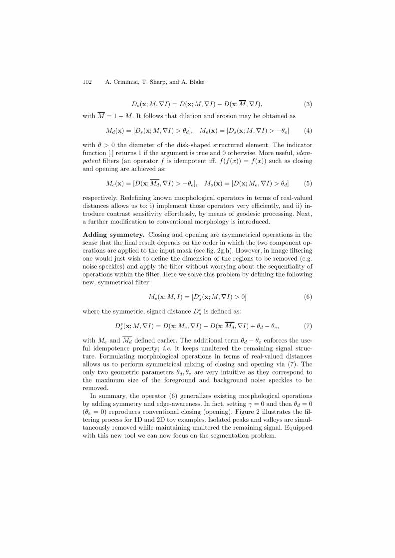
Ds(x; M,∇I) = D(x; M,∇I) − D(x; M,∇I), (3)

with M = 1 − M . It follows that dilation and erosion may be obtained as

Md(x) = [Ds(x; M,∇I) > θd], Me(x) = [Ds(x; M,∇I) > −θe] (4)

with θ > 0 the diameter of the disk-shaped structured element. The indicatorfunction [.] returns 1 if the argument is true and 0 otherwise. More useful, idem-potent filters (an operator f is idempotent iff. f(f(x)) = f(x)) such as closingand opening are achieved as:

Mc(x) = [D(x; Md,∇I) > −θe], Mo(x) = [D(x; Me,∇I) > θd] (5)

respectively. Redefining known morphological operators in terms of real-valueddistances allows us to: i) implement those operators very efficiently, and ii) in-troduce contrast sensitivity effortlessly, by means of geodesic processing. Next,a further modification to conventional morphology is introduced.

Adding symmetry. Closing and opening are asymmetrical operations in thesense that the final result depends on the order in which the two component op-erations are applied to the input mask (see fig. 2g,h). However, in image filteringone would just wish to define the dimension of the regions to be removed (e.g.noise speckles) and apply the filter without worrying about the sequentiality ofoperations within the filter. Here we solve this problem by defining the followingnew, symmetrical filter:

Ms(x; M, I) = [Dss(x; M,∇I) > 0] (6)

where the symmetric, signed distance Dss is defined as:

Dss(x; M,∇I) = D(x; Me,∇I) − D(x; Md,∇I) + θd − θe, (7)

with Me and Md defined earlier. The additional term θd − θe enforces the use-ful idempotence property; i.e. it keeps unaltered the remaining signal struc-ture. Formulating morphological operations in terms of real-valued distancesallows us to perform symmetrical mixing of closing and opening via (7). Theonly two geometric parameters θd, θe are very intuitive as they correspond tothe maximum size of the foreground and background noise speckles to beremoved.

In summary, the operator (6) generalizes existing morphological operationsby adding symmetry and edge-awareness. In fact, setting γ = 0 and then θd = 0(θe = 0) reproduces conventional closing (opening). Figure 2 illustrates the fil-tering process for 1D and 2D toy examples. Isolated peaks and valleys are simul-taneously removed while maintaining unaltered the remaining signal. Equippedwith this new tool we can now focus on the segmentation problem.


Fig. 2. Symmetric filtering in 1D and 2D. (a) Input, binary 1D signal M . (b) Theinitial signed distance Ds. (c) The two further unsigned distances for selected valuesof θd, θe. (d) The final signed distance Ds

s. (e) The filtered mask Ms(x;M). Some ofthe peaks and valleys of M(x) have been removed while maintaining the integrity ofthe remaining signal. For simplicity of explanation here no image gradient is used. Nowlet’s look at a 2D example. (f) Original 2D mask M , (g) mask after closing, (h) afteropening, (i) resulting mask Ms after our symmetric filtering. (j) The distance Ds(x)for the input 2D mask in (f). (k) The final distance Ds

s(x) for θd = 10 and θe = 11.The intersection of Ds

s(x) with the xy plane through 0 results in the filtered mask Ms

shown in (i). The parameters θd and θe are fixed in all (f,...,i).

4 Segmentation Via Restricted Energy Minimization

The binary segmentation problem addressed here is cast as minimizing an energyof type

E(z, α) = U(z, α) + λV (z, α) (8)

with z the image data and α the per-pixel labeling, with αn ∈ {Fg, Bg}. Thesubscript n indexes the pixels and Fg (Bg) indicates foreground (background).The unary potential U is defined as the sum of pixel-wise likelihoods of the formU(z, α) = −∑

n log p(zn|αn); and the data-dependent pairwise term is V (z, α) =−∑

m,n∈N [αn = αm] exp (−|zn − zm|/η). Here we use 8-neighborhood cliques N .Flux may also be incorporated in (8) as a further unary term.

Sub-modular energies of the form (8) can be minimized exactly by min-cut.However, in image segmentation, finding the global minimum of such energymakes sense only provided that the energy model correctly captures the statisticsof natural images. Recent work has shown that this is often not the case [8]. It hasbeen observed that often local energy minima correspond to segmentations whichare more accurate (compared to ground truth) than that yielded by the globalminimum. Thus, a technique that can find good local minima efficiently becomesvaluable. This section describes such an approximate and efficient technique.Later we will also show how such algorithm can be applied to energy models ofa more general nature than the one in (8).


Fig. 3. Filter behaviour in the presence of weak unaries. (a) Input unaries(green for Fg and red for Bg), with large uncertain areas (in grey). (b) Magnitude ofgradient of input image. (c) Computed segmentation boundary (white curve) for asmall value of θd = θe. (d) As in (c) but for large θ. Larger values of θ yield smoothersegmentation boundaries in the presence of weak edges and/or weak unaries. In con-trast, strong gradients “lock” the segmentation in place.

Key to our algorithm is the minimization of the energy in (8) by efficientsearch of the solution α∗ over a restricted, parametrized 2D manifold of all pos-sible segmentations. Let us define θ = (θd, θe) ∈ S, with S ⊂ R

2. As describedearlier, given a value of θ the geodesic operator (6) has the property of remov-ing isolated regions (with dimensions < θ) from foreground and background inbinary images. Therefore, if we can adapt our filter to work on real-valued unar-ies, then for different values of θ different levels of spatial smoothness would beobtained and thus different energy values. The segmentation we are after is

α∗ = α(θ∗), with θ∗ = arg minθ∈S

E(z, α(θ)).

Next we focus on the details of the GeoS algorithm.

Segmentation proposals. In a binary segmentation problem, given the real-valued log likelihood ratio: L(x) = log p(zn(x)|αn(x) = Fg) − log p(zn(x)|αn(x) =Bg) we redefine the mask M(x) ∈ [0, 1] as a log-odds map M(x) = σ(L(x)) withσ(.) the sigmoid transformation σ(L) = 1/(1 + exp(−L/μ)) 3. The distance (1)then becomes:

D(x; M,∇I) = minx′∈Ψ

(d(x,x′) + νM(x′)) (9)

with d(.) as in (2). ν (trained discriminatively) establishes the mapping betweenthe unary beliefs and the spatial distances. Different segmentations are achievedfor different values of θ via (6). Please refer to [20] for related work on (nongeodesic) generalized distance transforms.

Figure 3 illustrates the effect of applying our filter (6) to weak, real-valuedunaries. Larger values of θ not only tend to remove isolated islands (as illustratedearlier) but also produce smoother segmentation boundaries, in the presence ofweak contrast and/or uncertain unaries. Furthermore, strong edges “lock” thesegmentation in place. In summary, our filter produces segmentations which aresmooth, edge-aligned and agree with the unaries. Thus the filter is ideally suitedto be used for the generation of plausible segmentation hypotheses.3 In all experiments in this paper the value of μ is fixed to μ = 5.


Energy minimization. We now search for the value θ∗ corresponding tothe lowest energy EGeoS = E(z, α(θ∗)). For each value of θ the segmentationoperation in (6) requires 4 unsigned distance transforms. Thus, a naıve exhaus-tive search for Nd × Ne values of θ would require 4 Nd Ne distance computa-tions. However, it is easy to show that by pre-computing distances the load isreduced to only 2 + Nd + Ne operations 4, with an associated memory over-head. All of the above distance transforms are independent of each other andcan be computed in parallel on appropriate hardware. Therefore, in a machinewith Nc processors (cores) the total time T taken to run exhaustive search isT = (2 + (Nd + Ne)/Nc) t, with t the unit time required for each unsigned dis-tance transform (9). An economical gradient descent optimization strategy mayalso be employed here. Comparative efficiency results are presented in section 5.

Selecting the search space. An important question at this point is howto choose the search space S. As discussed earlier, θ are intuitive parameterswhich represent the maximum size of the regions to be removed. Therefore, Smust depend on the image resolution and on the spatial extent of noisy regionswithin the unary signal. Unless otherwise stated, for the approximately VGA-sized images used in this paper we have fixed S = {5, 6, ..., 15} × {5, 6, ..., 15}(and thus Nd = Ne = 10).

Estimating the segmentation posterior. Computing the full CRF poste-rior p(α) = 1/Zp exp (−E(α)/σp) is impractical [5]. However, importance sam-pling [21] allows us to approximate p(α) with its Monte Carlo mean p(α). Theproposal distribution q(α) can be computed as q(α) = 1/Zq exp (−E(α(θ))/σq),∀θ ∈ S (and q(α) = 0 ∀θ /∈ S). Then pq

N (α) = 1/n∑n

i=1 p(α(Θi))/q(α(Θi)),with the N samples Θi generated from a uniform prior over S. Since S is a small,quantized 2D space, in practice Θi are generated deterministically by exploringthe entire S. The parameters σq , σp are trained discriminatively from hundredsof manually-labelled trimaps (e.g. fig. 4d). The estimated CRF posterior pq

N (α)is used in fig. 4c”’,d”’ to compute the segmentation mean α =

∫α αpq

N (α)dαand the associated variance Λα. In interactive video segmentation, the quantityΛα may for instance be used to detect unstable segmentations and ask the userto improve the appearance models by adding more strokes. Proposals sampledfrom S may also be fused together via QPBO [22].

Exploring more complex energy models. In contrast to graph-cut, here theenergy and its minimization algorithm are decoupled. This fact is advantageoussince now the choice of class of energies is no longer dominated by considerationsof tractability. Our technique can thus be applied to more complex energy modelsthan the one in (8). As an example, below we consider energies containing globalterms:

E(z, α) = U(z, α) + λV (z, α) + κG(z, α) (10)

The global soft constraint G cannot be written as a sum of unary and pairwiseterms [23,24]. G captures global properties of image regions and can be used,

4 The distance Ds need be computed only once per image as it does not depend on θ.


e.g. to encourage constraints on areas, global appearance, shape or context. Forexample in [23] G = G(h1, h2) is defined as a divergence between region his-tograms hi. General energy models of this kind have not been used much in theliterature because of the lack of appropriate optimization techniques [25]. How-ever, their usefulness is clear, and finding even approximate, efficient solutionsis important. Results of this kind are presented in the next section.

5 Results and Applications

This section validates GeoS with respect to accuracy and efficiency. Qualitativeand quantitative results on interactive and automatic image and video segmen-tation are presented.

Interactive image segmentation. Figure 4 shows a first example of interac-tive segmentation on a difficult standard test image showing camouflage [26]. Theenergy is defined as in (8). In this and all interactive segmentation examples, theunaries (fig. 4c) are obtained by: i) computing histograms over the RGB spacequantized into 323 bins from the user provided strokes, and ii) evaluating the Fgand Bg likelihoods on all image pixels. As expected the GeoS MAP segmentationin fig. 4c’ looks like a version of the unaries but with higher spatial smoothnessof labels. The GeoS solution is very similar to the min-cut one (fig. 4c”). Thesegmentation mean α and variance are also computed. The mean image α canbe thought of as an automatically computed trimap.

Computational efficiency. Here we compare the run times of GeoS and min-cut. For min-cut we use the public implementation in [28] and also our ownimplementation which has been optimized for grid graphs. GeoS has been imple-mented using SSE2 assembly instructions, exploiting cache efficiency and multi-threading for optimal performance. The data-level parallelism (SSE2) is madepossible by noting that four of the five terms in the equation in fig. 12 are inde-pendent of the current scan-line. All experiments are run on an Intel Core2 Duodesktop with 3GB RAM and 2 × 2.6GHz CPU cores.

Figure 5 plots the run time curves obtained when segmenting the “llama” im-age as a function of image size. Both min-cut curves show a slightly “superlinear”behavior, while GeoS is linear. On a 1600 × 1200 image GeoS (Nc = 4, Nd =Ne = 10) produces a 12-fold speed-up with respect to min-cut. On-line videosegmentation may be achieved by gradient descent because of the high temporalcorrelation of the energy in consecutive frames (cf. fig.5c, denoted “g.d.”). Using2 steps of gradient descent on 2 × 2 grids (typical values) produces a 21-foldspeed-up. Geos’ efficiency gain increases non-linearly for larger resolutions. Forinstance, on a 25Mpix image the GeoS (Nc = 4, Nd = Ne = 10) produces a33-fold speed-up and gradient-descent GeoS a 60-fold speed-up with respect tomin-cut. Finally, while min-cut’s run times depend on the quality of the unaries(the more uncertain, the slower the minimization) GeoS has a fixed running cost,thus making its behaviour more predictable.


Fig. 4. GeoS v min-cut for interactive segmentation. (a) Input image.(b) userprovided Fg and Bg strokes, (c) corresponding unaries (green for Fg, red for Bg andgrey for uncertain). (d) ground truth segmentation (zoomed). (e) energy E(α(θ)),with the computed minimum marked in red. (f) The distance Ds

s corresponding tothe optimum θ∗. (g) The proposal distribution q(α(θ)). (c’,d’) Resulting GeoS MAPsegmentation α∗ and corresponding Fg layer. (c”,d”) Min-cut segmentation on thesame energy. (c”’) GeoS mean segmentation α, see text. Uncertain pixels are shownin grey. (d”’) corresponding GeoS variance (dark for high variance).

Fig. 5. Run time comparisons. (a) Run times for min-cut and GeoS for varyingimage size. Circles indicate our measurements. Associated uncertainties have been es-timated by assuming Gaussian noise on the measurements [27]. Min-cut [28] fails torun on images larger than 1600 × 1200, thus yielding larger uncertainty for higher res-olutions. (b) as in (a), zoomed into the highlighted region. Min-cut shows a slightlysuperlinear behaviour while GeoS is linear with a small slope. For large resolutionsGeoS can be up to 60 times faster than min-cut. (c) Run-times for 1600× 1200 resolu-tion. Even for relatively low resolution images GeoS is considerably faster than min-cut.Identical energies are used for all four algorithms compared in this figure.


Fig. 6. Interactive image segmentation. (a) Original test images: “sponge”, “per-son” and “flower” from the standard test database in [8] (approx. VGA sized); (b)unaries computed from the user scribbles provided in [8]; (c) GeoS segmentations. (d)min-cut segmentations for the same energy as in (c), corresponding to a single iter-ation of GrabCut [26]. More iterations as in [26] help reduce the amount of manualinteraction. (e) Percentage of differently classified pixels, see text.

When comparing GeoS with the algorithm in [29], GeoS yielded a roughly 30-fold speed-up factor while avoiding connectivity issues. Besides, the algorithmin [9,29] is designed for interactive segmentation only.

Segmentation accuracy. Figure 6 presents segmentation results on the stan-dard test images used in [8]. To quantify the difference in segmentation qualitybetween min-cut and GeoS we could use the relative difference between theminimum energy found, i.e. δ(EGeoS , Emin) = (EGeoS − Emin)/Emin, as in [8].However, this is not a good measure since adding a constant term ΔE to theenergy would not change the output segmentation while it would affect δ. Thusδ can be made very small by choosing a very large Δ. Here we chose to comparethe GeoS and min-cut segmentations to each other and to the manually labelledground truth by counting the number of differently classified pixels.

Results for the four example images encountered so far are reported in fig. 6e.In each case the optimum value of λ (learned discriminatively for min-cut) wasused. The min-cut and GeoS results are very close visually and quantitatively,with the number of differently labelled pixels well below 1% of the image area.The largest difference is for the “llama” image where the furry outline makesboth solutions equally likely. All segmentations are also very close to the groundtruth. The three GeoS segmentations in fig. 6c were obtained in < 10ms each(to be compared with the much larger timings reported in [8]).

Contrast sensitivity. In fig. 7 contrast-sensitivity enables thin protrusions tobe segmented correctly, despite the absence of flux in the energy. Contrast isespecially important with weaker unaries such as shown in fig. 3 and fig. 8. Infig. 8b,b’, using patches to compute stereo likelihoods [3] causes their misalign-ment with respect to the foreground boundary. Using γ > 0 in GeoS encourages


Fig. 7. The effect of contrast on thin structures. (a) Two input images. (b) unar-ies (from user strokes); (c) GeoS mean segmentation with no contrast. The smoothnessprior makes thin protrusions (e.g. the sheep legs or the planes missiles) uncertain (grey).(d) GeoS mean segmentation with contrast enabled. Now the contrast-sensitive pair-wise term correctly pulls the aeroplane and sheep thin protrusions in the foreground.(e) GeoS MAP segmentation for the contrast-sensitive energy in (d).

Fig. 8. Segmentation results in the presence of weak, stereo unaries. (a,a’)Frames from two stereo videos. (b,b’) Stereo likelihoods, with large uncertain areas (ingrey). (c,c’) GeoS segmentation, with no contrast sensitivity. (d,d’) As in (c,c’) butwith contrast sensitivity. Now the segmentation accurately follows the person’s outline.

Fig. 9. Exploiting global constraints. (a) Original test image; (b) user providedFg and Bg strokes; (c) corresponding unaries; (d) min-cut segmentation with κ = 0;The circular traffic sign is missed out. (e) GeoS segmentation on same energy as in(d); (f) GeoS segmentation on energy with global constraint G = |AreaFg/Area− 0.7|.

the segmentation to follow the person’s silhouette correctly (fig. 8d,d’). Next weexperiment with more complex energies, containing global terms.

Exploiting global energy constraints. The example in fig. 9 shows the ef-fect of the global constraint G in (10). Energies of the kind in (10) cannot beminimized by min-cut. In the segmentations in fig. 9d,e (where κ = 0) thecircular weight limit sign is missed. This problem is corrected in fig. 9f whichuses the energy (10) (with k > 0). The additional global term G is defined


as G = |AreaFg/Area − 0.7| to encourage the Fg region to cover about 70%of the image area. Similar results are obtained on this image by imposing softconstraints on global statistics of appearance or shape (see also [30]).

Segmenting n-dimensional data. Geodesic transforms and thus GeoS caneasily be extended to more than 2 dimensions. Figure 10 shows an exampleof segmentation of the space-time volume defined by a time-lapse video of agrowing flower. Figure 11 shows segmentation of 3D MRI data. In each casebrush strokes applied in two frames suffice to define good unaries. Individualorgans are highlighted in fig. 11 by repeated segmentation (see also [31]).

Fig. 10. Batch, space-time segmentation of video. (a) Three frames of a time-lapse video of a growing flower. (b, c, d) Three views of the segmented “video-cube”.GeoS segmentation is achieved directly in the space-time volume of the video.

Fig. 11. Segmentation of 3D, medical data. (a) Some of the 294 512× 512 inputgrey-scale slices from a patient’s torso. (b,c,d) GeoS segmentation results. Bones, heartand aorta have been accurately separated from the remaining soft tissue, directly inthe 3D volume. Different organs have been coloured to aid visual inspection.

Fig. 12. Efficient geodesic distance transform. See appendix.


6 Conclusion

This paper has presented GeoS, a new algorithm for the efficient segmentationof n-D images and videos. The key contribution is an approximate energy mini-mization technique which finds the segmentation solution by economical searchwithin a restricted space. Such space is populated by good, spatially-smooth,contrast-sensitive solution hypotheses generated by our new, efficient geodesicoperator. The algorithm’s reduced search space, contiguous memory access andintrinsic parallelism account for its efficiency even for high resolution data.

Extensive comparisons between GeoS and min-cut show comparable accuracy;with GeoS running many times faster and being able to handle more generalenergies.

References

1. Boykov, J., Jolly, M.P.: Interactive graph cuts for optimal boundary and regionsegmentation of objects in n-D images. In: IEEE ICCV (2001)

2. Rother, C., Kolmogorov, V., Blake, A.: Grabcut: Interactive foreground extractionusing iterated graph cuts. In: ACM Trans. on Graphics (SIGGRAPH) (2004)

3. Kolmogorov, V., Criminisi, A., Blake, A., Cross, G., Rother, C.: Bilayer segmen-tation of binocular stereo video. In: IEEE CVPR (2005)

4. Criminisi, A., Cross, G., Blake, A., Kolmogorov, V.: Bilayer segmentation of livevideo. In: IEEE CVPR (2006)

5. Kohli, P., Torr, P.H.S.: Measuring uncertainty in Graph Cut solutions. In: ECCV(2006)

6. Kolmogorov, V., Zabih, R.: Multi-camera scene reconstruction via graph cuts. In:ECCV (2002)

7. Sinop, A.K., Grady, L.: A seeded image segmentation framework unifying graphcuts and random walker which yields a new algorithm. In: IEEE ICCV (2007)

8. Szeliski, R., Zabih, R., Scharstein, D., Veksler, O., Kolmogorov, V., Agarwala, A.,Tappen, M., Rother, C.: A comparative study of energy minimization methods formarkov random fields. In: ECCV (2006)

9. Bai, X., Sapiro, G.: A geodesic framework for fast interactive image and videosegmentation and matting. In: IEEE ICCV (2007)

10. Komodakis, N., Tziritas, G., Paragios, N.: Fast, approximately optimal solutionsfor single and dynamic MRFs. In: IEEE CVPR (2007)

11. Lempitsky, V., Rother, C., Blake, A.: Logcut - efficient graph cut optimization formarkov random fields. In: IEEE ICCV, Rio (2007)

12. Juan, O., Boykov, J.: Active graph cuts. In: IEEE CVPR (2006)13. Kohli, P., Torr, P.: Dynamic graph cuts for efficient inference in markov random

fields. PAMI (2007)14. Fabbri, R., Costa, L., Torrelli, J., Bruno, O.: 2d euclidean distance transform al-

gorithms: A comparative survey. ACM Computing Surveys 40 (2008)15. Jones, M., Baerentzen, J., Sramek, M.: 3d distance fields: a survey of techniques

and applications. IEEE Trans. on Visualization and Computer Graphics 12 (2006)16. Borgefors, G.: Distance transformations in digital images. Computer Vision,

Graphics and Image Processing (1986)17. Sethian, J.A.: Fast marching methods. SIAM Rev. 41 (1999)


18. Toivanen, P.J.: New geodesic distance transforms for gray-scale images. PatternRecognition Letters 17, 437–450 (1996)

19. Yatziv, L., Bartesaghi, A., Sapiro, G.: O(n) implementation of the fast marchingalgorithm. Journal of Computational Physics 212, 393–399 (2006)

20. Felzenszwalb, P.F., Huttenlocher, D.P.: Pictorial structures for object recognition.IJCV 61 (2005)

21. Ripley, B.D.: Stochastic Simulation. Wiley and Sons, Chichester (1987)22. Rother, C., Kolmogorov, V., Lempitsky, V.T., Szummer, M.: Optimizing binary

MRFs via extended roof duality. In: IEEE CVPR (2007)23. Rother, C., Kolmogorov, V., Minka, T., Blake, A.: Cosegmentation of image pairs

by histogram matching - incor. a global constraint into MRFs. In: CVPR (2006)24. Kolmogorov, V., Boykov, J., Rother, C.: Applications of parametric maxflow in

computer vision. In: IEEE ICCV, Rio (2007)25. Kolmogorov, V., Zabih, R.: What energy functions can be minimized via graph

cuts? IEEE Trans. PAMI 26 (2004)26. Blake, A., Rother, C., Brown, M., Perez, P., Torr, P.: Interactive image segmenta-

tion using an adaptive GMMRF model. In: ECCV (2004)27. Bishop, C.M.: Pattern Recognition and machine Learning. Springer, Heidelberg

(2006)28. http://www.adastral.ucl.ac.uk/∼vladkolm29. Bai, X., Sapiro, G.: A geodesic framework for fast interactive image and video

segmentation and matting. Technical Report 2185, Institute of Mathematics andIts Applications, Univ. Minnesota Preprint Series(2008)

30. Cremers, D., Osher, S.J., Soatto, S.: Kernel density estimation and intrinsic align-ment for shape priors in level set segmentation. IJCV 69 (2006)

31. Yatziv, L., Sapiro, G.: Fast image and video colorization using chrominance blend-ing. IEEE Trans. on Image Processing 15 (2006)

Appendix – Fast Geodesic Distance Transform

Given a map M(x) ∈ [0, 1], in the forward pass the map is scanned with a 3× 3kernel from the top-left to the bottom-right corner and the intermediate functionC(x) is iteratively constructed as illustrated in fig. 12. The north-west, north,north-east and west components of the image gradient ∇I are used. The ρ1 andρ2 local distances are usually set to ρ1 = 1 and ρ2 =

√2. In the backward pass

the algorithm proceeds from the bottom-right to the top-left corner and appliesthe backward kernel to C(x) to produce the final distance D(x) (cf. fig. 1).Larger kernels produce better approximations to the exact distance.

http://www.adastral.ucl.ac.uk/~vladkolm

geos: geodesic image segmentation - microsoft.com geodesic image segmentation antonio criminisi,...

Documents