Mesh R-CNN

Georgia Gkioxari Jitendra Malik Justin Johnson

Facebook AI Research (FAIR)

Abstract

Rapid advances in 2D perception have led to systemsthat accurately detect objects in real-world images. How-ever, these systems make predictions in 2D, ignoring the 3Dstructure of the world. Concurrently, advances in 3D shapeprediction have mostly focused on synthetic benchmarksand isolated objects. We unify advances in these two areas.We propose a system that detects objects in real-world im-ages and produces a triangle mesh giving the full 3D shapeof each detected object. Our system, called Mesh R-CNN,augments Mask R-CNN with a mesh prediction branch thatoutputs meshes with varying topological structure by firstpredicting coarse voxel representations which are convertedto meshes and refined with a graph convolution network op-erating over the mesh’s vertices and edges. We validateour mesh prediction branch on ShapeNet, where we out-perform prior work on single-image shape prediction. Wethen deploy our full Mesh R-CNN system on Pix3D, wherewe jointly detect objects and predict their 3D shapes.

1. IntroductionThe last few years have seen rapid advances in 2D ob-

ject recognition. We can now build systems that accuratelyrecognize objects [19, 30, 55, 61], localize them with 2Dbounding boxes [13, 47] or masks [18], and predict 2D key-point positions [3, 18, 65] in cluttered, real-world images.Despite their impressive performance, these systems ignoreone critical fact: that the world and the objects within it are3D and extend beyond the XY image plane.

At the same time, there have been significant advances in3D shape understanding with deep networks. A menagerieof network architectures have been developed for differ-ent 3D shape representations, such as voxels [5], point-clouds [8], and meshes [69]; each representation carriesits own benefits and drawbacks. However, this diverse andcreative set of techniques has primarily been developed onsynthetic benchmarks such as ShapeNet [4] consisting ofrendered objects in isolation, which are dramatically lesscomplex than natural-image benchmarks used for 2D objectrecognition like ImageNet [52] and COCO [37].

We believe that the time is ripe for these hitherto dis-

Input Image 2D Recognition

3D Meshes 3D Voxels

Figure 1. Mesh R-CNN takes an input image, predicts objectinstances in that image and infers their 3D shape. To capture di-versity in geometries and topologies, it first predicts coarse voxelswhich are refined for accurate mesh predictions.

tinct research directions to be combined. We should striveto build systems that (like current methods for 2D percep-tion) can operate on unconstrained real-world images withmany objects, occlusion, and diverse lighting conditions butthat (like current methods for 3D shape prediction) do notignore the rich 3D structure of the world.

In this paper we take an initial step toward this goal. Wedraw on state-of-the-art methods for 2D perception and 3Dshape prediction to build a system which inputs a real-worldRGB image, detects the objects in the image, and outputs acategory label, segmentation mask, and a 3D triangle meshgiving the full 3D shape of each detected object.

Our method, called Mesh R-CNN, builds on the state-of-the-art Mask R-CNN [18] system for 2D recognition, aug-menting it with a mesh prediction branch that outputs high-resolution triangle meshes.

Our predicted meshes must be able to capture the 3Dstructure of diverse, real-world objects. Predicted meshesshould therefore dynamically vary their complexity, topol-ogy, and geometry in response to varying visual stimuli.However, prior work on mesh prediction with deep net-works [23, 57, 69] has been constrained to deform from

1

arX

iv:1

906.

0273

9v1

[cs

.CV

] 6

Jun

201

9

Figure 2. Example predictions from Mesh R-CNN on Pix3D. Us-ing initial voxel predictions allows our outputs to vary in topology;converting these predictions to meshes and refining them allows usto capture fine structures like tabletops and chair legs.

fixed mesh templates, limiting them to fixed mesh topolo-gies. As shown in Figure 1, we overcome this limitationby utilizing multiple 3D shape representations: we first pre-dict coarse voxelized object representations, which are con-verted to meshes and refined to give highly accurate meshpredictions. As shown in Figure 2, this hybrid approach al-lows Mesh R-CNN to output meshes of arbitrary topologywhile also capturing fine object structures.

We benchmark our approach on two datasets. First,we evaluate our mesh prediction branch on ShapeNet [4],where our hybrid approach of voxel prediction and meshrefinement outperforms prior work by a large margin. Sec-ond, we deploy our full Mesh R-CNN system on the recentPix3D dataset [60] which aligns 395 models of IKEA fur-niture to real-world images featuring diverse scenes, clut-ter, and occlusion. To date Pix3D has primarily beenused to evalute shape predictions for models trained onShapeNet, using perfectly cropped, unoccluded image seg-ments [41, 60, 73], or synthetic rendered images of Pix3Dmodels [76]. In contrast, using Mesh R-CNN we are thefirst to train a system on Pix3D which can jointly detect ob-jects of all categories and estimate their full 3D shape.

2. Related WorkOur system inputs a single RGB image and outputs a set

of detected object instances, with a triangle mesh for eachobject. Our work is most directly related to recent advancesin 2D object recognition and 3D shape prediction. We alsodraw more broadly from work on other 3D perception tasks.2D Object Recognition Methods for 2D object recogni-tion vary both in the type of information predicted per ob-ject, and in the overall system architecture. Object de-tectors output per-object bounding boxes and category la-bels [12, 13, 36, 38, 46, 47]; Mask R-CNN [18] additionallyoutputs instance segmentation masks. Our method extendsthis line of work to output a full 3D mesh per object.Single-View Shape Prediction Recent approaches use avariety of shape representations for single-image 3D recon-struction. Some methods predict the orientation [10, 20] or

3D pose [31, 44, 66] of known shapes. Other approachespredict novel 3D shapes as sets of 3D points [8, 34],patches [15, 70], or geometric primitives [9, 64, 67]; othersuse deep networks to model signed distance functions [42].These methods can flexibly represent complex shapes, butrely on post-processing to extract watertight mesh outputs.

Some methods predict regular voxel grids [5, 71, 72];while intuitive, scaling to high-resolution outputs requirescomplex octree [50, 62] or nested shape architectures [49].

Others directly output triangle meshes, but are con-strained to deform from fixed [56, 57, 69] or retrieved meshtemplates [51], limiting the topologies they can represent.

Our approach uses a hybrid of voxel prediction and meshdeformation, enabling high-resolution output shapes thatcan flexibly represent arbitrary topologies.

Some methods reconstruct 3D shapes without 3D anno-tations [23, 25, 48, 68, 75]. This is an important direction,but at present we consider only the fully supervised casedue to the success of strong supervision for 2D perception.Multi-View Shape Prediction There is a broad line of workon multi-view reconstruction of objects and scenes, fromclassical binocular stereo [17, 53] to using shape priors [1,2, 6, 21] and modern learning techniques [24, 26, 54]. Inthis work, we focus on single-image shape reconstruction.3D Inputs Our method inputs 2D images and predicts se-mantic labels and 3D shapes. Due to the increasing avail-abilty of depth sensors, there has been growing interest inmethods predicting semantic labels from 3D inputs such asRGB-D images [16, 58] and pointclouds [14, 32, 45, 59,63]. We anticipate that incorporating 3D inputs into ourmethod could improve the fidelity of our shape predictions.Datasets Advances in 2D perception have been driven bylarge-scale annotated datasets such as ImageNet [52] andCOCO [37]. Datasets for 3D shape prediction have laggedtheir 2D counterparts due to the difficulty of collecting 3Dannotations. ShapeNet [4] is a large-scale dataset of CADmodels which are rendered to give synthetic images. TheIKEA dataset [33] aligns CAD models of IKEA objects toreal-world images; Pix3D [60] extends this idea to a largerset of images and models. Pascal3D [74] aligns CAD mod-els to real-world images, but it is unsuitable for shape recon-struction since its train and test sets share the same small setof models. KITTI [11] annotates outdoor street scenes with3D bounding boxes, but does not provide shape annotations.

3. MethodOur goal is to design a system that inputs a single image,

detects all objects, and outputs a category label, boundingbox, segmentation mask and 3D triangle mesh for each de-tected object. Our system must be able to handle clutteredreal-world images, and must be trainable end-to-end. Ouroutput meshes should not be constrained to a fixed topol-

Figure 3. System overview of Mesh R-CNN. We augment Mask R-CNN with 3D shape inference. The voxel branch predicts a coarseshape for each detected object which is further deformed with a sequence of refinement stages in the mesh refinement branch.

ogy in order to accommodate a wide variety of complexreal-world objects. We accomplish these goals by marryingstate-of-the-art 2D perception with 3D shape prediction.

Specifically, we build on Mask R-CNN [18], a state-of-the-art 2D perception system. Mask R-CNN is an end-to-end region-based object detector. It inputs a single RGBimage and outputs a bounding box, category label, and seg-mentation mask for each detected object. The image isfirst passed through a backbone network (e.g. ResNet-50-FPN [35]); next a region proposal network (RPN) [47]gives object proposals which are processed with object clas-sification and mask prediction branches.

Part of Mask R-CNN’s success is due to RoIAlignwhich extracts region features from image features whilemaintaining alignment between the input image and fea-tures used in the final prediction branches. We aim to main-tain similar feature alignment when predicting 3D shapes.

We infer 3D shapes with a novel mesh predictor, com-prising a voxel branch and a mesh refinement branch. Thevoxel branch first estimates a coarse 3D voxelization of anobject, which is converted to an initial triangle mesh. Themesh refinement branch then adjusts the vertex positions ofthis initial mesh using a sequence of graph convolution lay-ers operating over the edges of the mesh.

The voxel branch and mesh refinement branch are ho-mologous to the existing box and mask branches of Mask R-CNN. All take as input image-aligned features correspond-ing to RPN proposals. The voxel and mesh losses, describedin detail below, are added to the box and mask losses and thewhole system is trained end-to-end. The output is a set ofboxes along with their predicted object scores, masks and3D shapes. We call our system Mesh R-CNN, which is il-lustrated in Figure 3.

We now describe our mesh predictor, consisting of thevoxel branch and mesh refinement branch, along with itsassociated losses in detail.

3.1. Mesh Predictor

At the core of our system is a mesh predictor which re-ceives convolutional features aligned to an object’s bound-ing box and predicts a triangle mesh giving the object’s full3D shape. Like Mask R-CNN, we maintain correspondencebetween the input image and features used at all stages ofprocessing via region- and vertex-specific alignment opera-tors (RoIAlign and VertAlign). Our goal is to captureinstance-specific 3D shapes of all objects in an image. Thus,each predicted mesh must have instance-specific topology(genus, number of vertices, faces, connected components)and geometry (vertex positions).

We predict varying mesh topologies by deploying a se-quence of shape inference operations. First, the voxelbranch makes bottom-up voxelized predictions of each ob-ject’s shape, similar to Mask R-CNN’s mask branch. Thesepredictions are converted into meshes and adjusted by themesh refinement head, giving our final predicted meshes.

The output of the mesh predictor is a triangle mesh T =(V, F ) for each object. V = {vi ∈ R3} is the set of vertexpositions and F ⊆V×V×V is a set of triangular faces.

3.1.1 Voxel Branch

The voxel branch predicts a grid of voxel occupancy proba-bilities giving the course 3D shape of each detected object.It can be seen as a 3D analogue of Mask R-CNN’s mask pre-diction branch: rather than predicting a M ×M grid givingthe object’s shape in the image plane, we instead predict aG×G×G grid giving the object’s full 3D shape.

Like Mask R-CNN, we maintain correspondence be-tween input features and predicted voxels by applying asmall fully-convolutional network [39] to the input featuremap resulting from RoIAlign. This network produces afeature map with G channels giving a column of voxel oc-cupancy scores for each position in the input.

World Space Prediction Space

K-1

KImage plane

ZXY

Znear

Zfar

Figure 4. Predicting voxel occupancies aligned to the image planerequires an irregularly-shaped voxel grid. We achieve this effectby making voxel predictions in a space that is transformed bythe camera’s (known) intrinsic matrix K. Applying K−1 trans-forms our predictions back to world space. This results in frustum-shaped voxels in world space.

Maintaining pixelwise correspondence between the im-age and our predictions is complex in 3D since objects be-come smaller as they recede from the camera. As shown inFigure 4, we account for this by using the camera’s (known)intrinsic matrix to predict frustum-shaped voxels.Cubify: Voxel to Mesh The voxel branch produces a 3Dgrid of occupancy probabilities giving the coarse shape ofan object. In order to predict more fine-grained 3D shapes,we wish to convert these voxel predictions into a trianglemesh which can be passed to the mesh refinement branch.

We bridge this gap with an operation called cubify. Itinputs voxel occupancy probabilities and a threshold for bi-narizing voxel occupancy. Each occupied voxel is replacedwith a cuboid triangle mesh with 8 vertices, 18 edges, and12 faces. Shared vertices and edges between adjacent occu-pied voxels are merged, and shared interior faces are elim-inated. This results in a watertight mesh whose topologydepends on the voxel predictions.

Cubify must be efficient and batched. This is nottrivial and we provide technical implementation details ofhow we achieve this in Appendix A. Alternatively march-ing cubes [40] could extract an isosurface from the voxelgrid, but is significantly more complex.Voxel Loss The voxel branch is trained to minimize thebinary cross-entropy between predicted voxel occupancyprobabilities and true voxel occupancies.

3.1.2 Mesh Refinement Branch

The cubified mesh from the voxel branch only provides acoarse 3D shape, and it cannot accurately model fine struc-tures like chair legs. The mesh refinement branch processesthis initial cubified mesh, refining its vertex positions witha sequence of refinement stages. Similar to [69], each re-finement stage consists of three operations: vertex align-ment, which extracts image features for vertices; graph con-volution, which propagates information along mesh edges;and vertex refinement, which updates vertex positions. Eachlayer of the network maintains a 3D position vi and a fea-ture vector fi for each mesh vertex.

Vertex Alignment yields an image-aligned feature vectorfor each mesh vertex1. We use the camera’s intrinsic matrixto project each vertex onto the image plane. Given a featuremap, we compute a bilinearly interpolated image feature ateach projected vertex position [22].

In the first stage of the mesh refinement branch,VertAlign outputs an initial feature vector for each ver-tex. In subsequent stages, the VertAlign output is con-catenated with the vertex feature from the previous stage.Graph Convolution [29] propagates information alongmesh edges. Given input vertex features {fi} it computesupdated features f ′i = ReLU

(W0fi +

∑j∈N (i)W1fj

)where N (i) gives the i-th vertex’s neighbors in the mesh,and W0 and W1 are learned weight matrices. Each stage ofthe mesh refinement branch uses several graph convolutionlayers to aggregate information over local mesh regions.Vertex Refinement computes updated vertex positionsv′i = vi + tanh(Wvert [fi; vi]) where Wvert is a learnedweight matrix. This updates the mesh geometry, keeping itstopology fixed. Each stage of the mesh refinement branchterminates with vertex refinement, producing an intermedi-ate mesh output which is further refined by the next stage.Mesh Losses Defining losses that operate natively on trian-gle meshes is challenging, so we instead use loss functionsdefined over a finite set of points. We represent a mesh witha pointcloud by densely sampling its surface. Consequently,a pointcloud loss approximates a loss over shapes.

Similar to [57], we use a differentiable mesh samplingoperation to sample points (and their normal vectors) uni-formly from the surface of a mesh. To this end, we im-plement an efficient batched sampler; see Appendix B fordetails. We use this operation to sample a pointcloud P gt

from the ground-truth mesh, and a pointcloud P i from eachintermediate mesh prediction from our model.

Given two pointclouds P , Q with normal vectors, letΛP,Q = {(p, arg minq ‖p − q‖) : p ∈ P} be the set ofpairs (p, q) such that q is the nearest neighbor of p inQ, andlet up be the unit normal to point p. The chamfer distancebetween pointclouds P and Q is given by

Lcham(P,Q) = |P |−1∑

(p,q)∈ΛP,Q

‖p− q‖2 + |Q|−1∑

(q,p)∈ΛQ,P

‖q − p‖2 (1)

and the (absolute) normal distance is given by

Lnorm(P,Q) = −|P |−1∑

(p,q)∈ΛP,Q

|up · uq | − |Q|−1∑

(q,p)∈ΛQ,P

|uq · up|. (2)

The chamfer and normal distances penalize mismatchedpositions and normals between two pointclouds, but min-imizing these distances alone results in degenerate meshes(see Figure 5). High-quality mesh predictions require addi-tional shape regularizers: To this end we use an edge lossLedge(V,E) = 1

|E|∑

(v,v′)∈E ‖v− v′‖2 where E ⊆ V × V

1 Vertex alignment is called perceptual feature pooling in [69]

are the edges of the predicted mesh. Alternatively, a Lapla-cian loss [7] also imposes smoothness constraints.

The mesh loss of the i-th stage is a weighted sum ofLcham(P i, P gt), Lnorm(P i, P gt) and Ledge(V

i, Ei). Themesh refinement branch is trained to minimize the mean ofthese losses across all refinement stages.

4. ExperimentsWe benchmark our mesh predictor on ShapeNet [4],

where we compare with state-of-the-art approaches. Wethen evaluate our full Mesh R-CNN for the task of 3D shapeprediction in the wild on the challenging Pix3D dataset [60].

4.1. ShapeNet

ShapeNet [4] provides a collection of 3D shapes, repre-sented as textured CAD models organized into semantic cat-egories following WordNet [43], and has been widely usedas a benchmark for 3D shape prediction. We use the subsetof ShapeNetCore.v1 and rendered images from [5]. Eachmesh is rendered from up to 24 random viewpoints, givingRGB images of size 137× 137. We use the train / test splitsprovided by [69], which allocate 35,011 models (840,189images) to train and 8,757 models (210,051 images) to test;models used in train and test are disjoint. We reserve 5% ofthe training models as a validation set.

The task on this dataset is to input a single RGB imageof a rendered ShapeNet model on a blank background, andoutput a 3D mesh for the object in the camera coordinatesystem. During training the system is supervised with pairsof images and meshes.Evaluation We adopt evaluation metrics used in recentwork [56, 57, 69]. We sample 10k points uniformly at ran-dom from the surface of predicted and ground-truth meshes,and use them to compute Chamfer distance (Equation 1),Normal consistency, (one minus Equation 2), and F1τ atvarious distance thresholds τ , which is the harmonic meanof the precision at τ (fraction of predicted points within τ ofa ground-truth point) and the recall at τ (fraction of ground-truth points within τ of a predicted point). Lower is betterfor Chamfer distance; higher is better for all other metrics.

With the exception of normal consistency, these metricsdepend on the absolute scale of the meshes. In Table 1 wefollow [69] and rescale by a factor of 0.57; for all otherresults we follow [8] and rescale so the longest edge of theground-truth mesh’s bounding box has length 10.Implementation Details Our backbone feature extractor isResNet-50 pretrained on ImageNet. Since images depict asingle object, the voxel branch receives the entire conv5 3feature map, bilinearly resized to 24 × 24, and predicts a48 × 48 × 48 voxel grid. The VertAlign operator con-catenates features from conv2 3, conv3 4, conv4 6,and conv5 3 before projecting to a vector of dimension

Chamfer (↓) F1τ (↑) F12τ (↑)N3MR [25] 2.629 33.80 47.723D-R2N2 [5] 1.445 39.01 54.62PSG [8] 0.593 48.58 69.78Pixel2Mesh [69]† 0.591 59.72 74.19MVD [56] - 66.39 -GEOMetrics [57] - 67.37 -Pixel2Mesh [69]‡ 0.444 68.94 80.75Ours (Best) 0.284 75.83 86.63Ours (Pretty) 0.366 70.70 82.59

Table 1. Single-image shape reconstruction results on ShapeNet,using the evaluation protocol from [69]. For [69], † are resultsreported in their paper and ‡ is the model released by the authors.

128. The mesh refinement branch has three stages, eachwith six graph convolution layers (of dimension 128) or-ganized into three residual blocks. We train for 25 epochsusing Adam [27] with learning rate 10−4 and 32 images perbatch on 8 Tesla V100 GPUs. We set the cubify thresh-old to 0.2 and weight the losses with λvoxel = 1, λcham = 1,λnorm = 0, and λedge = 0.5.Baselines We compare with previously published methodsfor single-image shape prediction. N3MR [25] is a weaklysupervised approach that fits a mesh via a differentiable ren-derer without 3D supervision. 3D-R2N2 [5] and MVD [56]output voxel predictions. PSG [8] predicts point-clouds.Appendix D additionally compares with OccNet [42].

Pixel2Mesh [69] predicts meshes by deforming and sub-dividing an initial ellipsoid. GEOMetrics [57] extends [69]with adaptive face subdivision. Both are trained to mini-mize Chamfer distances; however [69] computes it usingpredicted mesh vertices, while [57] uses points sampled uni-formly from predicted meshes. We adopt the latter as it bet-ter matches test-time evaluation. Unlike ours, these meth-ods can only predict connected meshes of genus zero.

The training recipe and backbone architecture varyamong prior work. Therefore for a fair comparison with ourmethod we also compare against several ablated versions ofour model (see Appendix C for exact details):

• Voxel-Only: A version of our method that terminateswith the cubified meshes from the voxel branch.

• Pixel2Mesh+: We reimplement Pixel2Mesh [69]; weoutperform their original model due to a deeper back-bone, better training recipe, and minimizing Chamfer onsampled rather than vertex positions.

• Sphere-Init: Similar to Pixel2Mesh+, but initializes froma high-resolution sphere mesh, performing three stagesof vertex refinement without subdivision.

• Ours (light): Uses a smaller nonresidual mesh refinementbranch with three graph convolution layers per stage. Wewill adopt this lightweight design on Pix3D.

Voxel-Only is essentially a version of our method thatomits the mesh refinement branch, while Pixel2Mesh+ andSphere-Init omit the voxel prediction branch.

Full Test Set Holes Test SetChamfer(↓) Normal F10.1 F10.3 F10.5 |V | |F | Chamfer(↓) Normal F10.1 F10.3 F10.5 |V | |F |

Pixel2Mesh [69]‡ 0.205 0.736 33.7 80.9 91.7 2466±0 4928±0 0.272 0.689 31.5 75.9 87.9 2466±0 4928±0Voxel-Only 0.916 0.595 7.7 33.1 54.9 1987±936 3975±1876 0.760 0.592 8.2 35.7 59.5 2433±925 4877±1856

Bes

t

Sphere-Init 0.132 0.711 38.3 86.5 95.1 2562±0 5120±0 0.138 0.705 40.0 85.4 94.3 2562±0 5120±0Pixel2Mesh+ 0.132 0.707 38.3 86.6 95.1 2562±0 5120±0 0.137 0.696 39.3 85.5 94.4 2562±0 5120±0Ours (light) 0.133 0.725 39.2 86.8 95.1 1894±925 3791±1855 0.130 0.723 41.6 86.7 94.8 2273±899 4560±1805Ours 0.133 0.729 38.8 86.6 95.1 1899±928 3800±1861 0.130 0.725 41.7 86.7 94.9 2291±903 4595±1814

Pret

ty

Sphere-Init 0.175 0.718 34.5 82.2 92.9 2562±0 5120±0 0.186 0.684 34.4 80.2 91.7 2562±0 5120±0Pixel2Mesh+ 0.175 0.727 34.9 82.3 92.9 2562±0 5120±0 0.196 0.685 34.4 79.9 91.4 2562±0 5120±0Ours (light) 0.176 0.699 34.8 82.4 93.1 1891±924 3785±1853 0.178 0.688 36.3 82.0 92.4 2281±895 4576±1798Ours 0.171 0.713 35.1 82.6 93.2 1896±928 3795±1861 0.171 0.700 37.1 82.4 92.7 2292±902 4598±1812

Table 2. We report results both on the full ShapeNet test set (left), as well as a subset of the test set consisting of meshes with visibleholes (right). We compare our full model with several ablated version: Voxel-Only omits the mesh refinement head, while Sphere-Init andPixel2Mesh+ omit the voxel head. We show results both for Best models which optimize for metrics, as well as Pretty models that strikea balance between shape metrics and mesh quality (see Figure 5); these two categories of models should not be compared. We also reportthe number of vertices |V | and faces |F | in predicted meshes (mean±std). ‡ refers to the released model by the authors.

Input Image Without Ledge(best)

With Ledge(pretty)

Figure 5. Training without the edge length regularizer Ledgeresults in degenerate predicted meshes that have many overlap-ping faces. Adding Ledge eliminates this degeneracy but results inworse agreement with the ground-truth as measured by standardmetrics such as Chamfer distance.

Best vs Pretty As previously noted in [69] (Section 4.1),standard metrics for shape reconstruction are not well-correlated with mesh quality. Figure 5 shows that mod-els trained without shape regularizers give meshes that arepreferred by metrics despite being highly degenerate, withirregularly-sized faces and many self-intersections. Thesedegenerate meshes would be difficult to texture, and maynot be useful for downstream applications.

Due to the strong effect of shape regularizers on bothmesh quality and quantitative metrics, we suggest onlyquantitatively comparing methods trained with the sameshape regularizers. We thus train two versions of all ourShapeNet models: a Best version with λedge = 0 to serve asan upper bound on quantitative performance, and a Prettyversion that strikes a balance between quantitative perfor-mance and mesh quality by setting λedge = 0.5.Comparison with Prior Work Table 1 compars our Prettyand Best models with prior work on shape prediction froma single image. We use the evaluation protocol from [69],

Imag

ePi

xel2

Mes

h+O

urs

Figure 6. Pixel2Mesh+ predicts meshes by deforming an initialsphere, so it cannot properly model objects with holes. In contrastour method can model objects with arbitrary topologies.

using a 0.57 mesh scaling factor and threshold value τ =10−4 on squared Euclidean distances. For Pixel2Mesh, weprovide the performance reported in their paper [69] as wellas the performance of their open-source pretrained model.Table 1 shows that we outperform prior work by a widemargin, validating the design of our mesh predictor.Ablation Study Fairly comparing with prior work is chal-lenging due to differences in backbone networks, losses,and shape regularizers. For a controlled evaluation, we ab-late variants using the same backbone and training recipe,shown in Table 2. ShapeNet is dominated by simple ob-jects of genus zero. Therefore we evaluate both on the en-tire test set and on a subset consisting of objects with one ormore holes (Holes Test Set) 2. In this evaluation we removethe ad-hoc scaling factor of 0.57, and we rescale meshes sothe longest edge of the ground-truth mesh’s bounding boxhas length 10, following [8]. We compare the open-source

2We annotated 3075 test set models and flagged whether they containedholes. This resulted in 17% (or 534) of the models being flagged. SeeAppendix F for more details and examples.

Pix3D S1 APbox APmask APmesh chair sofa table bed desk bkcs wrdrb tool misc |V | |F |Voxel-Only 93.7 87.1 6.8 0.1 3.6 4.6 3.1 2.0 38.0 7.9 0.0 1.8 2354±706 4717±1423

Pixel2Mesh+ 91.9 86.8 40.4 29.9 63.3 42.9 39.6 33.6 42.2 47.1 36.9 27.7 2562±0 5120±0

Sphere-Init 92.1 88.2 40.5 33.3 61.9 46.2 40.2 31.0 47.6 34.4 45.5 24.0 2562±0 5120±0

Mesh R-CNN (ours) 92.5 87.5 55.4 48.3 76.4 68.0 51.5 47.2 71.3 60.1 43.9 31.7 2367±698 4743±1406

# test instances 2440 2440 2440 1129 398 398 205 148 79 53 11 19

Pix3D S2

Voxel-Only 66.4 62.8 4.9 0.0 0.0 2.1 1.4 1.5 18.2 0.2 21.0 0.0 2346±630 4702±1269

Pixel2Mesh+ 67.1 60.8 23.7 22.4 69.4 13.0 42.5 8.6 26.7 1.1 29.6 0.0 2562±0 5120±0

Sphere-Init 65.9 61.3 24.8 24.6 73.3 13.6 40.2 5.7 31.2 1.5 33.2 0.0 2562±0 5120±0

Mesh R-CNN (ours) 66.4 60.9 28.7 36.6 80.1 26.5 42.8 15.6 32.4 1.8 22.5 0.0 2358±633 4726±1274

# test instances 2368 2368 2368 778 506 398 219 205 85 135 22 20

Table 3. Performance on Pix3D S1 & S2. We report mean APbox, APmask and APmesh, as well as per category APmesh. All AP performancesare in %. The Voxel-Only baseline outputs the cubified voxel predictions. The Sphere-Init and Pixel2Mesh+ baselines deform an initialsphere and thus are limited to making predictions homeomorphic to spheres. Our Mesh R-CNN is flexible and can capture arbitrarytopologies. We outperform the baselines consistently while predicting meshes with fewer number of vertices and faces.

CNN init # refine steps APbox APmask APmesh

COCO 3 92.5 87.5 55.4IN 3 91.8 85.5 52.9

COCO 2 92.0 86.9 54.5COCO 1 92.7 87.8 52.4

Table 4. Ablations of Mesh R-CNN on Pix3D.

Pixel2Mesh model against our ablations in this evaluationsetting. Pixel2Mesh+ (our reimplementation of [69]) sig-nificantly outperforms the original due to an improved train-ing recipe and deeper backbone.

We draw several conclusions from Table 2: (a) On theFull Test Set, our full model and Pixel2Mesh+ perform onpar. However, on the Holes Test Set, our model dominatesas it is able to predict topologically diverse shapes whilePixel2Mesh+ is restricted to make predictions homeomor-phic to spheres, and cannot model holes or disconnectedcomponents (see Figure 6). This discrepancy is quantita-tively more salient on Pix3D (Section 4.2) as it containsmore complex shapes. (b) Sphere-Init and Pixel2Mesh+

perform similarly overall (both Best and Pretty), suggest-ing that mesh subdivision may be unnecessary for strongquantitative performance. (c) The deeper residual meshrefinement architecture (inspired by [69]) performs on-parwith the lighter non-residual architecture, motivating ouruse of the latter on Pix3D. (d) Voxel-Only performs poorlycompared to methods that predict meshes, demonstratingthat mesh predictions better capture fine object structure.(e) Each Best model outperforms its corresponding Prettymodel; this is expected since Best is an upper bound onquantitative performance.

4.2. Pix3D

We now turn to Pix3D [60], which consists of 10069real-world images and 395 unique 3D models. Here the taskis to jointly detect and predict 3D shapes for known objectcategories. Pix3D does not provide standard train/test splits,so we prepare two splits of our own.

Our first split, S1, randomly allocates 7500 images fortraining and 2500 for testing. Despite the small num-ber of unique object models compared to ShapeNet, S1 ischallenging since the same model can appear with varyingappearance (e.g. color, texture), in different orientations,under different lighting conditions, in different contexts,and with varying occlusion. This is a stark contrast withShapeNet, where objects appear against blank backgrounds.

Our second split, S2, is even more challenging: we en-sure that the 3D models appearing in the train and test setsare disjoint. Success on this split requires generalizationnot only to the variations present in S1, but also to novel 3Dshapes of known categories: for example a model may seekitchen chairs during training but must recognize armchairsduring testing. This split is possible due to Pix3D’s uniqueannotation structure, and poses interesting challenges forboth 2D recognition and 3D shape prediction.Evaluation We adopt metrics inspired by those used for 2Drecognition: APbox, APmask and APmesh. The first two arestandard metrics used for evaluating COCO object detectionand instance segmentation at intersection-over-union (IoU)0.5. APmesh evalutes 3D shape prediction: it is the meanarea under the per-category precision-recall curves for F10.3

at 0.53. Pix3D is not exhaustively annotated, so for evalua-tion we only consider predictions with box IoU > 0.3 witha ground-truth region. This avoids penalizing the model forcorrect predictions corresponding to unannotated objects.

We compare predicted and ground-truth meshes in thecamera coordinate system. Our model assumes known cam-era intrinsics for VertAlign. Mesh R-CNN predicts ob-ject positions in the image plane, but it cannot resolve thefundamental scale / depth ambiguity along the Z-axis. Dur-ing evaluation we therefore match the depth extent (Znearand Zfar) of our predictions to the ground-truth shape. Fu-ture work might predict depth extents based on shape priors.

3A mesh prediction is considered a true-positive if its predicted label iscorrect, it is not a duplicate detection, and its F10.3 > 0.5

Figure 7. Examples of Mesh R-CNN predictions on Pix3D. Mesh R-CNN detects multiple objects per image, reconstructs fine details suchas chair legs, and predicts varying and complex mesh topologies for objects with holes such as bookcases and tables.

Pix3D S1 gt APbox APmask APmesh chair sofa table bed desk bkcs wrdrb tool misc Chamfer (↓) Normal F10.1 F10.3 F10.5

Voxel-Only 100.0 90.7 6.7 0.0 2.8 3.9 1.1 1.1 36.7 12.1 2.3 0.6 1.28 0.57 9.9 37.3 56.1Pixel2Mesh+ 100.0 92.0 35.1 22.4 55.6 42.2 32.6 32.5 44.6 38.6 29.1 18.4 1.30 0.70 16.4 51.0 68.4Sphere-Init 100.0 92.4 33.4 23.7 52.0 41.6 34.9 26.4 42.0 32.9 33.2 13.8 1.30 0.69 16.8 51.4 68.8Mesh R-CNN (ours) 100.0 92.1 49.1 38.8 67.0 63.4 38.9 47.2 78.3 53.7 33.2 21.1 1.11 0.71 18.7 56.4 73.5

Table 5. Performance on Pix3D S1 on ground-truth regions. In addition to the mean APbox, APmask, APmesh, and per category APmesh wereport Chamfer distance, Normal consistency and F1 scores.

Implementation details We use ResNet-50-FPN [35] asthe backbone CNN; the box and mask branches are identi-cal to Mask R-CNN. The voxel branch resembles the maskbranch, but the pooling resolution is decreased to 12 (vs. 14for masks) due to memory constraints giving 24× 24× 24voxel predictions. We adopt the lightweight design for themesh refinement branch from Section 4.1. We train for12 epochs with a batch size of 64 per image on 8 TeslaV100 GPUs (two images per GPU). We use SGD with mo-mentum, linearly increasing the learning rate from 0.002 to0.02 over the first 1K iterations, then decaying by a fac-tor of 10 at 8K and 10K iterations. We initialize from amodel pretrained for instance segmentation on COCO. Weset the cubify threshold to 0.2 and the loss weights toλvoxel = 3.0, λcham = 1.0, λnorm = 0.1 and λedge = 0.5 anduse weight decay 10−4; detection loss weights are identicalto Mask R-CNN.Comparison to Baselines As discussed in Section 1, weare the first to tackle joint detection and shape inference inthe wild on Pix3D. To validate our approach we comparewith ablated versions of Mesh R-CNN, replacing our fullmesh predictor with Voxel-Only, Pixel2Mesh+, and Sphere-Init branches (see Section 4.1). All baselines otherwise usethe same architecture and training recipe.

Table 3 (top) shows the performance on S1. We observethat: (a) Mesh R-CNN outperforms all baselines, improvingover the next-best by 14.9% APmesh overall and across mostcategories; Tool and Misc4 have very few test-set instances(11 and 19 respectively), so their AP is noisy. (b) MeshR-CNN shows large gains vs. Sphere-Init for objects withcomplex shapes such as bookcase (+23.7%), table (+21.8%)and chair (+15.0%). (c) Voxel-Only performs very poorly– this is expected due to its coarse predictions.

Table 3 (bottom) shows the performance on the morechallenging S2 split. Here we observe: (a) The overall per-

4Misc consists of objects such as fire hydrant, picture frame, vase, etc.

formance on 2D recognition (APbox , APmask ) drops signifi-cantly compared to S1, signifying the difficulty of recogniz-ing novel shapes in the wild. (b) Mesh R-CNN outperformsall baselines for shape prediction for all categories excepttool. (c) Absolute performance on wardrobe and misc issmall for all methods due to significant shape disparity be-tween models in train and test.

Table 4 compares pretraining on COCO vs ImageNet,and compares different architectures for the mesh predictor.COCO vs ImageNet initialization significantly improves 2Drecognition (APmask 87.5 vs. 85.5) and 3D shape predic-tion (APmesh 55.4 vs. 52.9). Shape prediction is signifi-cantly degraded when using only one mesh refinement stage(APmesh 55.4 vs. 52.4).

In Table 5 we evaluate our trained models using ground-truth object regions, thus assuming perfect bounding-box detection. Absolute performance on shape recon-struction (Chamfer, Normal, etc.) is significantly lowerthan on ShapeNet, demonstrating the difficulty of Pix3D.APmesh drops by a few points for all models compared toTable 3 (top), possibly because tight object regions, devoidof context, are not ideal for 3D shape prediction, which canbe amplified when training on imperfect region proposals.

Figures 2 and 7 show example predictions from MeshR-CNN. Our method can detect multiple objects per im-age, reconstruct fine details such as chair legs, and predictvarying and complex mesh topologies for objects with holessuch as bookcases and desks.

DiscussionWe propose Mesh R-CNN, a novel system for joint 2D

perception and 3D shape inference. We validate our ap-proach on ShapeNet and show its merits on Pix3D. MeshR-CNN is a first attempt at 3D shape prediction in the wild.Despite the lack of large supervised data, e.g. compared toCOCO, Mesh R-CNN shows promising results.

Acknowledgements We would like to thank Kaiming He,Piotr Dollar, Leonidas Guibas, Manolis Savva and ShubhamTulsiani for valuable discussions. We would also like tothank Lars Mescheder and Thibault Groueix for their help.

Appendix

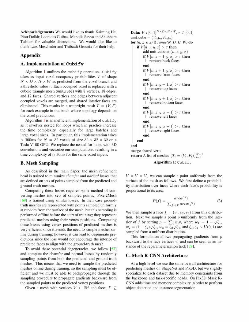
A. Implementation of CubifyAlgorithm 1 outlines the cubify operation. Cubify

takes as input voxel occupancy probabilities V of shapeN × D × H ×W as predicted from the voxel branch anda threshold value τ . Each occupied voxel is replaced with acuboid triangle mesh (unit cube) with 8 vertices, 18 edges,and 12 faces. Shared vertices and edges between adjacentoccupied voxels are merged, and shared interior faces areeliminated. This results in a watertight mesh T = (V, F )for each example in the batch whose topology depends onthe voxel predictions.

Algorithm 1 is an inefficient implementation of cubifyas it involves nested for loops which in practice increasethe time complexity, especially for large batches andlarge voxel sizes. In particular, this implementation takes> 300ms for N = 32 voxels of size 32 × 32 × 32 on aTesla V100 GPU. We replace the nested for loops with 3Dconvolutions and vectorize our computations, resulting in atime complexity of ≈ 30ms for the same voxel inputs.

B. Mesh SamplingAs described in the main paper, the mesh refinement

head is trained to minimize chamfer and normal losses thatare defined on sets of points sampled from the predicted andground-truth meshes.

Computing these losses requires some method of con-verting meshes into sets of sampled points. Pixel2Mesh[69] is trained using similar losses. In their case ground-truth meshes are represented with points sampled uniformlyat random from the surface of the mesh, but this sampling isperformed offline before the start of training; they representpredicted meshes using their vertex positions. Computingthese losses using vertex positions of predicted meshes isvery efficient since it avoids the need to sample meshes on-line during training; however it can lead to degenerate pre-dictions since the loss would not encourage the interior ofpredicted faces to align with the ground-truth mesh.

To avoid these potential degeneracies, we follow [57]and compute the chamfer and normal losses by randomlysampling points from both the predicted and ground-truthmeshes. This means that we need to sample the predictedmeshes online during training, so the sampling must be ef-ficient and we must be able to backpropagate through thesampling procedure to propagate gradients backward fromthe sampled points to the predicted vertex positions.

Given a mesh with vertices V ⊂ R3 and faces F ⊆

Data: V : [0, 1]N×D×H×W , τ ∈ [0, 1]unit cube = (Vcube, Fcube)for (n, z, y, x) ∈ range(N, D, H, W) do

if V [n, z, y, x] > τ thenadd unit cube at (n, z, y, x)if V [n, z − 1, y, x] > τ then

remove back facesendif V [n, z + 1, y, x] > τ then

remove front facesendif V [n, z, y − 1, x] > τ then

remove top facesendif V [n, z, y + 1, x] > τ then

remove bottom facesendif V [n, z, y, x− 1] > τ then

remove left facesendif V [n, z, y, x+ 1] > τ then

remove right facesend

endendmerge shared vertsreturn A list of meshes {Ti = (Vi, Fi)}N−1i=0

Algorithm 1: Cubify

V × V × V , we can sample a point uniformly from thesurface of the mesh as follows. We first define a probabil-ity distribution over faces where each face’s probability isproportional to its area:

P (f) =area(f)∑

f ′∈F area(f ′)(3)

We then sample a face f = (v1, v2, v3) from this distribu-tion. Next we sample a point p uniformly from the inte-rior of f by setting p =

∑i wivi where w1 = 1 −

√ξ1,

w2 = (1− ξ2)√ξ1, w3 = ξ2

√ξ1, and ξ1, ξ2 ∼ U(0, 1) are

sampled from a uniform distribution.This formulation allows propagating gradients from p

backward to the face vertices vi and can be seen as an in-stance of the reparameterization trick [28].

C. Mesh R-CNN ArchitectureAt a high level we use the same overall architecture for

predicting meshes on ShapeNet and Pix3D, but we slightlyspecialize to each dataset due to memory constraints fromthe backbone and task-specific heads. On Pix3D Mask R-CNN adds time and memory complexity in order to performobject detection and instance segmentation.

Index Inputs Operation Output shape(1) Input conv2 3 features 35× 35× 256(2) Input conv3 4 features 18× 18× 512(3) Input conv4 6 features 9× 9× 1024(4) Input conv5 3 features 5× 5× 2048(5) Input Input vertex features |V | × 128(6) Input Input vertex positions |V | × 3(7) (1), (6) VertAlign |V | × 256(8) (2), (6) VertAlign |V | × 512(9) (3), (6) VertAlign |V | × 1024

(10) (4), (6) VertAlign |V | × 2048(11) (7),(8),(9),(10) Concatenate |V | × 3840(12) (11) Linear(3840→ 128) |V | × 128(13) (5), (6), (12) Concatenate |V | × 259(14) (13) ResGraphConv(259→ 128) |V | × 128(15) (14) 2× ResGraphConv(128→ 128) |V | × 128(16) (15) GraphConv(128→ 3) |V | × 3(17) (16) Tanh |V | × 3(18) (6), (17) Addition |V | × 3

Table 6. Architecture for a single residual mesh refinement stageon ShapeNet. For ShapeNet we follow [69] and use residualblocks of graph convolutions: ResGraphConv(D1 → D2) con-sists of two graph convolution layers (each preceeded by ReLU)and an additive skip connection, with a linear projection if the in-put and output dimensions are different. The output of the refine-ment stage are the vertex features (15) and the updated vertex po-sitions (18). The first refinement stage does not take input vertexfeatures (5), so for this stage (13) only concatenates (6) and (12).

Index Inputs Operation Output shape(1) Input Image 137× 137× 3(2) (1) ResNet-50 conv2 3 35× 35× 256(3) (2) ResNet-50 conv3 4 18× 18× 512(4) (3) ResNet-50 conv4 6 9× 9× 1024(5) (4) ResNet-50 conv5 3 5× 5× 2048(6) (5) Bilinear interpolation 24× 24× 2048(7) (6) Voxel Branch 48× 48× 48(8) (7) cubify |V | × 3, |F | × 3(9) (2), (3), (4), (5), (8) Refinement Stage 1 |V | × 3, |F | × 3

(10) (2), (3), (4), (5), (9) Refinement Stage 2 |V | × 3, |F | × 3(11) (2), (3), (4), (5), (10) Refinement Stage 3 |V | × 3, |F | × 3

Table 7. Overall architecture for our ShapeNet model. Since wedo not predict bounding boxes or masks, we feed the conv5 3features from the whole image into the voxel branch. The archi-tecture for the refinement stage is shown in Table 6, and the archi-tecture for the voxel branch is shown in Table 9.

ShapeNet. The overall architecture of our ShapeNet modelis shown in Table 7; the architecture of the voxel branch isshown in Table 9.

We consider two different architectures for the mesh re-finement network on ShapeNet. Our full model as wellas our Pixel2Mesh+ and Sphere-Init baselines use meshrefinement stages with three residual blocks of two graphconvolutions each, similar to [69]; the architecture of thesestages is shown in Table 6. We also consider a shallowerlightweight design which uses only three graph convolutionlayers per stage, omitting residual connections and insteadconcatenating the input vertex positions before each graphconvolution layer. The architecture of this lightweight de-sign is shown in Table 8.

Index Inputs Operation Output shape(1) Input conv2 3 features 35× 35× 256(2) Input conv3 4 features 18× 18× 512(3) Input conv4 6 features 9× 9× 1024(4) Input conv5 3 features 5× 5× 2048(5) Input Input vertex features |V | × 128(6) Input Input vertex positions |V | × 3(7) (1), (6) VertAlign |V | × 256(8) (2), (6) VertAlign |V | × 512(9) (3), (6) VertAlign |V | × 1024(10) (4), (6) VertAlign |V | × 2048(11) (7),(8),(9),(10) Concatenate |V | × 3840(12) (11) Linear(3840→ 128) |V | × 128(13) (5), (6), (12) Concatenate |V | × 259(14) (13) GraphConv(259→ 128) |V | × 128(15) (6), (14) Concatenate |V | × 131(16) (15) GraphConv(131→ 128) |V | × 128(17) (6), (16) Concatenate |V | × 131(18) (17) GraphConv(131→ 128) |V | × 128(19) (18) Linear(128→ 3) |V | × 3(20) (19) Tanh |V | × 3(21) (6), (20) Addition |V | × 3

Table 8. Architecture for the nonresidual mesh refinement stageuse in the lightweight version of our ShapeNet models. EachGraphConv operation is followed by ReLU. The output of thestage are the vertex features (18) and updated vertex positions (21).The first refinement stage does not take input vertex features (5),so for this stage (13) only concatenates (6) and (12).

Index Inputs Operation Output shape(1) Input Image features V/2× V/2×D(2) (1) Conv(D → 256, 3× 3), ReLU V/2× V/2× 256(3) (2) Conv(256→ 256, 3× 3), ReLU V/2× V/2× 256(4) (3) TConv(256→ 256, 2× 2, 2), ReLU V × V × 256(5) (4) Conv(256→ V, 1× 1) V × V × V

Table 9. Architecture of our voxel prediction branch. ForShapeNet we use V = 48 and for Pix3D we use V = 24. TConvis a transpose convolution with stride 2.

As shown in Table 2, we found that these two archi-tectures perform similarly on ShapeNet even though thelightweight design uses half as many graph convolution lay-ers per stage. We therefore use the nonresidual design forour Pix3D models.Pix3D. The overall architecture of our full Mesh R-CNNsystem on Pix3D is shown in Table 10. The backbone,RPN, box branch, and mask branch are identical to Mask R-CNN [18]. The voxel branch is the same as in the ShapeNetmodels (see Table 9), except that we predict voxels at alower resolution (48×48×48 for ShapeNet vs. 24×24×24for Pix3D) due to memory constraints. Table 11 showsthe exact architecture of the mesh refinement stages for ourPix3D models.Baselines. The Voxel-Only baseline is identical to the fullmodel, except that it omits all mesh refinement branchesand terminates with the mesh resulting from cubify. OnShapeNet, the Voxel-Only baseline is trained with a batchsize of 64 (vs. a batch size of 32 for our full model); onPix3D it uses the same training recipe as our full model.

Index Inputs Operation Output shape(1) Input Input Image H ×W × 3(2) (1) Backbone: ResNet-50-FPN h× w × 256(3) (2) RPN h× w ×A× 4(4) (2),(3) RoIAlign 14× 14× 256(5) (4) Box branch: 2× downsample, Flatten, Linear(7 ∗ 7 ∗ 256→ 1024), Linear(1024→ 5C) C × 5(6) (4) Mask branch: 4× Conv(256→ 256, 3× 3), TConv(256→ 256, 2× 2, 2), Conv(256→ C, 1× 1) 28× 28× C(7) (2), (3) RoIAlign 12× 12× 256(8) (7) Voxel Branch 24× 24× 24(9) (8) cubify |V | × 3, |F | × 3

(10) (7), (9) Refinement Stage 1 |V | × 3, |F | × 3(11) (7), (10) Refinement Stage 2 |V | × 3, |F | × 3(12) (7), (11) Refinement Stage 3 |V | × 3, |F | × 3

Table 10. Overall architecture of Mesh R-CNN on Pix3D. The backbone, RPN, box, and mask branches are identical to Mask R-CNN.The RPN produces a bounding box prediction for each of the A anchors at each spatial location in the input feature map; a subset ofthese candidate boxes are processed by the other branches, but here we show only the shapes resulting from processing a single box forthe subsequent task-specific heads. Here C is the number of categories (10 = 9 + background for Pix3D); the box branch producesper-category bounding boxes and classification scores, while the mask branch produces per-category segmentation masks. TConv is atranspose convolution with stride 2. We use a ReLU nonlinearity between all Linear, Conv, and TConv operations. The architecture fo thevoxel branch is shown in Table 9, and the architecture of the refinement stages is shown in Table 11.

Index Inputs Operation Output shape(1) Input Backbone features h× w × 256(2) Input Input vertex features |V | × 128(3) Input Input vertex positions |V | × 3(4) (1), (3) VertAlign |V | × 256(5) (2), (3), (4) Concatenate |V | × 387(6) (5) GraphConv(387→ 128) |V | × 128(7) (3), (6) Concatenate |V | × 131(8) (7) GraphConv(131→ 128) |V | × 128(9) (3), (8) Concatenate |V | × 131

(10) (9) GraphConv(131→ 128) |V | × 128(11) (3), (10) Concatenate |V | × 131(12) (11) Linear(131→ 3) |V | × 3(13) (12) Tanh |V | × 3(14) (3), (13) Addition |V | × 3

Table 11. Architecture for a single mesh refinement stage onPix3D.

The Pixel2Mesh+ is our reimplementation of [69]. Thisbaseline omits the voxel branch; instead all images use anidentical inital mesh. The initial mesh is a level-2 icospherewith 162 vertices, 320 faces, and 480 edges which resultsfrom applying two face subdivision operations to a regu-lar icosahedron and projecting all resulting vertices onto asphere. For the Pixel2Mesh+ baseline, the mesh refinementstages are the same as our full model, except that we applya face subdivision operation prior to VertAlign in refine-ment stages 2 and 3.

Like Pixel2Mesh+, the Sphere-Init baseline omits thevoxel branch and uses an identical initial sphere mesh for allimages. However unlike Pixel2Mesh+ the initial mesh is alevel-4 icosphere with 2562 vertices, 5120 faces, and 7680edges which results from applying four face subdivivisonoperations to a regular icosahedron. Due to this large initialmesh, the mesh refinement stages are identical to our fullmodel, and do not use mesh subdivision.

Chamfer(↓) Normal F10.1 F10.3 F10.5 |V | |F |OccNet [42] 0.264 0.789 33.4 80.5 91.3 2499±60 4995±120

Bes

t Ours (light) 0.135 0.725 38.9 86.7 95.0 1978±951 3958±1906Ours 0.139 0.728 38.3 86.3 94.9 1985±960 3971±1924

Pret

ty Ours (light) 0.185 0.696 34.3 82.0 92.8 1976±956 3954±1916Ours 0.180 0.709 34.6 82.2 93.0 1982±961 3967±1926

Table 12. Comparison between our method and Occpancy Net-works (OccNet) [42] on ShapeNet. We use the same evaluationmetrics and setup as Table 2.

Pixel2Mesh+ and Sphere-Init both predict meshes withthe same number of vertices and faces, and with identicaltopologies; the only difference between them is whether allsubdivision operations are performed before the mesh re-finement branch (Sphere-Init) or whether mesh refinementis interleaved with mesh subdivision (Pixel2Mesh+). OnShapeNet, the Pixel2Mesh+ and Sphere-Init baselines aretrained with a batch size of 96; on Pix3D they use the sametraining recipe as our full model.

D. Comparison with Occupancy NetworksOccupancy Networks [42] (OccNet) also predict 2D

meshes with neural networks. Rather than outputing a meshdirectly from the neural network as in our approach, theytrain a neural network to compute a signed distance betweena query point in 3D space and the object boundary. At test-time a 3D mesh can be extracted from a set of query points.Like our approach, OccNets can also predict meshes withvarying topolgy per input instance.

Table 12 compares our approach with OccNet on theShapeNet test set. We obtained test-set predictions for Oc-cNet from the authors. Our method and OccNet are trainedon slightly different splits of the ShapeNet dataset, so we

Pixel2Mesh+ Mesh R-CNN

Figure 8. Qualitative comparisons between Pixel2Mesh+ andMesh R-CNN on Pix3D. Each row shows the same example forPixel2Mesh+ (first three columns) and Mesh R-CNN (last threecolumns), respectively. For each method, we show the input im-age along with the predicted 2D mask (chair, bookcase, table, bed)and box (in green) superimposed. We show the 3D mesh renderedon the input image and an additional view of the 3D mesh.

compare our methods on the intersection of our respectivetest splits. From Table 12 we see that OccNets achievehigher normal consistency than our approach; however boththe Best and Pretty versions of our model outperform Occ-Nets on all other metrics.

E. Pix3D: Visualizations and ComparisonsFigure 8 shows qualitative comparisons between

Pixel2Mesh+ and Mesh R-CNN. Pixel2Mesh+ is limitedto making predictions homeomorphic to spheres and thuscannot capture varying topologies, e.g. holes. In addi-tion, Pixel2Mesh+ has a hard time capturing high curva-tures, such as sharp table tops and legs. This is due to thelarge deformations required when starting from a sphere,which are not encouraged by the shape regularizers. On theother hand, Mesh R-CNN initializes its shapes with cubifiedvoxel predictions resulting in better initial shape represen-tations which require less drastic deformations.

F. ShapeNet Holes test setWe construct the ShapeNet Holes Test set by selecting

models from the ShapeNet test set that have visible holes

from any viewpoint. Figure 9 shows several input imagesfor randomly selected models from this subset. This test setis very challenging – many objects have small holes result-ing from thin structures; and some objects have holes whichare not visible from all viewpoints.

References[1] S. Y. Bao, M. Chandraker, Y. Lin, and S. Savarese. Dense

object reconstruction with semantic priors. In CVPR, 2013.2

[2] V. Blanz and T. Vetter. A morphable model for the synthesisof 3d faces. In SIGGRAPH, 1999. 2

[3] Z. Cao, T. Simon, S.-E. Wei, and Y. Sheikh. Realtimemulti-person 2D pose estimation using part affinity fields. InCVPR, 2017. 1

[4] A. X. Chang, T. A. Funkhouser, L. J. Guibas, P. Hanrahan,Q. Huang, Z. Li, S. Savarese, M. Savva, S. Song, H. Su,J. Xiao, L. Yi, and F. Yu. Shapenet: An information-rich 3dmodel repository. In CoRR 1512.03012, 2015. 1, 2, 5

[5] C. B. Choy, D. Xu, J. Gwak, K. Chen, and S. Savarese. 3D-R2N2: A unified approach for single and multi-view 3d ob-ject reconstruction. In ECCV, 2016. 1, 2, 5

[6] A. Dame, V. A. Prisacariu, C. Y. Ren, and I. Reid. Densereconstruction using 3d object shape priors. In CVPR, 2013.2

[7] M. Desbrun, M. Meyer, P. Schroder, and A. H. Barr. Im-plicit fairing of irregular meshes using diffusion and curva-ture flow. In SIGGRAPH, 1999. 5

[8] H. Fan, H. Su, and L. J. Guibas. A point set generation net-work for 3d object reconstruction from a single image. InCVPR, 2017. 1, 2, 5, 6

[9] S. Fidler, S. Dickinson, and R. Urtasun. 3d object detec-tion and viewpoint estimation with a deformable 3d cuboidmodel. In NeurIPS, 2012. 2

[10] D. F. Fouhey, A. Gupta, and M. Hebert. Data-driven 3Dprimitives for single image understanding. In ICCV, 2013. 2

[11] A. Geiger, P. Lenz, C. Stiller, and R. Urtasun. Vision meetsrobotics: The kitti dataset. In IJRR, 2013. 2

[12] R. Girshick. Fast R-CNN. In ICCV, 2015. 2[13] R. Girshick, J. Donahue, T. Darrell, and J. Malik. Rich fea-

ture hierarchies for accurate object detection and semanticsegmentation. In CVPR, 2014. 1, 2

[14] B. Graham, M. Engelcke, and L. van der Maaten. 3d se-mantic segmentation with submanifold sparse convolutionalnetworks. In CVPR, 2018. 2

[15] T. Groueix, M. Fisher, V. G. Kim, B. C. Russell, andM. Aubry. A papier-mache approach to learning 3d surfacegeneration. In CVPR, 2018. 2

[16] S. Gupta, R. Girshick, P. Arbelaez, and J. Malik. Learningrich features from rgb-d images for object detection and seg-mentatio. In ECCV, 2014. 2

[17] R. Hartley and A. Zisserman. Multiple view geometry incomputer vision. Cambridge university press, 2003. 2

[18] K. He, G. Gkioxari, P. Dollar, and R. Girshick. Mask R-CNN. In ICCV, 2017. 1, 2, 3, 10

Figure 9. Example input images for randomly selected models from the the Holes Test Set on ShapeNet. For each model we show threedifferent input images showing the model from different viewpoints. This set is extremely challenging – some models may have very smallholes (such as the holes in the back of the chair in the left model of the first row, or the holes on the underside of the table on the rightmodel of row 2), and some models may have holes which are not visible in all input images (such as the green chair in the middle of thefourth row, or the gray desk on the right of the ninth row).

[19] K. He, X. Zhang, S. Ren, and J. Sun. Deep residual learningfor image recognition. In CVPR, 2016. 1

[20] D. Hoiem, A. A. Efros, and M. Hebert. Geometric contextfrom a single image. In ICCV, 2005. 2

[21] C. Hne, N. Savinov, and M. Pollefeys. Class specific 3d ob-

ject shape priors using surface normals. In CVPR, 2014. 2[22] M. Jaderberg, K. Simonyan, A. Zisserman, et al. Spatial

transformer networks. In NeurIPS, 2015. 4[23] A. Kanazawa, S. Tulsiani, A. A. Efros, and J. Malik. Learn-

ing category-specific mesh reconstruction from image col-

lections. In ECCV, 2018. 1, 2[24] A. Kar, C. Hane, and J. Malik. Learning a multi-view stereo

machine. In NeurIPS, 2017. 2[25] H. Kato, Y. Ushiku, and T. Harada. Neural 3D mesh renderer.

In CVPR, 2018. 2, 5[26] A. Kendall, H. Martirosyan, S. Dasgupta, P. Henry,

R. Kennedy, A. Bachrach, and A. Bry. End-to-end learn-ing of geometry and context for deep stereo regression. InICCV, 2017. 2

[27] D. P. Kingma and J. Ba. Adam: A method for stochasticoptimization. In ICLR, 2015. 5

[28] D. P. Kingma and M. Welling. Auto-encoding variationalbayes. In ICLR, 2014. 9

[29] T. N. Kipf and M. Welling. Semi-supervised classificationwith graph convolutional networks. In ICLR, 2017. 4

[30] A. Krizhevsky, I. Sutskever, and G. Hinton. ImageNetclassification with deep convolutional neural networks. InNeurIPS, 2012. 1

[31] A. Kundu, Y. Li, and J. M. Rehg. 3d-rcnn: Instance-level3d object reconstruction via render-and-compare. In CVPR,2018. 2

[32] Y. Li, R. Bu, M. Sun, W. Wu, X. Di, and B. Chen. Pointcnn:Convolution on x-transformed points. In NeurIPS, 2018. 2

[33] J. J. Lim, H. Pirsiavash, and A. Torralba. Parsing IKEA Ob-jects: Fine Pose Estimation. In ICCV, 2013. 2

[34] C.-H. Lin, C. Kong, and S. Lucey. Learning efficient pointcloud generation for dense 3d object reconstruction. In AAAI,2018. 2

[35] T.-Y. Lin, P. Dollar, R. Girshick, K. He, B. Hariharan, andS. Belongie. Feature pyramid networks for object detection.In CVPR, 2017. 3, 8

[36] T.-Y. Lin, P. Goyal, R. Girshick, K. He, and P. Dollar. Focalloss for dense object detection. In ICCV, 2017. 2

[37] T.-Y. Lin, M. Maire, S. Belongie, J. Hays, P. Perona, D. Ra-manan, P. Dollr, and C. L. Zitnick. Microsoft COCO: Com-mon objects in context. ECCV, 2014. 1, 2

[38] W. Liu, D. Anguelov, D. Erhan, C. Szegedy, and S. Reed.SSD: Single shot multibox detector. In ECCV, 2016. 2

[39] J. Long, E. Shelhamer, and T. Darrell. Fully convolutionalnetworks for semantic segmentation. In CVPR, 2015. 3

[40] W. E. Lorensen and H. E. Cline. Marching cubes: A highresolution 3d surface construction algorithm. In SIGGRAPH.ACM, 1987. 4

[41] P. Mandikal, N. Murthy, M. Agarwal, and R. V. Babu. 3d-lmnet: Latent embedding matching for accurate and diverse3d point cloud reconstruction from a single image. In BMVC,2018. 2

[42] L. Mescheder, M. Oechsle, M. Niemeyer, S. Nowozin, andA. Geiger. Occupancy networks: Learning 3d reconstructionin function space. In CVPR, 2019. 2, 5, 11

[43] G. A. Miller. Wordnet: A lexical database for english. InCommun. ACM, 1995. 5

[44] G. Pavlakos, X. Zhou, A. Chan, K. G. Derpanis, and K. Dani-ilidis. 6-dof object pose from semantic keypoints. In ICRA,2017. 2

[45] C. R. Qi, L. Yi, H. Su, and L. J. Guibas. Pointnet++: Deephierarchical feature learning on point sets in a metric space.In NeurIPS, 2017. 2

[46] J. Redmon, S. Divvala, R. Girshick, and A. Farhadi. Youonly look once: Unified, real-time object detection. InCVPR, 2016. 2

[47] S. Ren, K. He, R. Girshick, and J. Sun. Faster R-CNN: To-wards real-time object detection with region proposal net-works. In NeurIPS, 2015. 1, 2, 3

[48] D. J. Rezende, S. A. Eslami, S. Mohamed, P. Battaglia,M. Jaderberg, and N. Heess. Unsupervised learning of 3dstructure from images. In NeurIPS, 2016. 2

[49] S. R. Richter and S. Roth. Matryoshka networks: Predicting3d geometry via nested shape layers. In CVPR, 2018. 2

[50] G. Riegler, A. Osman Ulusoy, and A. Geiger. Octnet: Learn-ing deep 3d representations at high resolutions. In CVPR,2017. 2

[51] J. Rock, T. Gupta, J. Thorsen, J. Gwak, D. Shin, andD. Hoiem. Completing 3d object shape from one depth im-age. In CVPR, 2015. 2

[52] O. Russakovsky, J. Deng, H. Su, J. Krause, S. Satheesh,S. Ma, Z. Huang, A. Karpathy, A. Khosla, M. Bernstein,A. C. Berg, and L. Fei-Fei. ImageNet Large Scale VisualRecognition Challenge. IJCV, 2015. 1, 2

[53] D. Scharstein and R. Szeliski. A taxonomy and evaluation ofdense two-frame stereo correspondence algorithms. IJCV,2002. 2

[54] T. Schmidt, R. Newcombe, and D. Fox. Self-supervised vi-sual descriptor learning for dense correspondence. In IEEERobotics and Automation Letters, 2017. 2

[55] K. Simonyan and A. Zisserman. Very deep convolutionalnetworks for large-scale image recognition. In ICLR, 2015.1

[56] E. Smith, S. Fujimoto, and D. Meger. Multi-view silhouetteand depth decomposition for high resolution 3d object repre-sentation. In NeurIPS, 2018. 2, 5

[57] E. J. Smith, S. Fujimoto, A. Romero, and D. Meger. GE-OMetrics: Exploiting geometric structure for graph-encodedobjects. In ICML, 2019. 1, 2, 4, 5, 9

[58] S. Song and J. Xiao. Deep Sliding Shapes for amodal 3Dobject detection in RGB-D images. In CVPR, 2016. 2

[59] H. Su, V. Jampani, D. Sun, S. Maji, E. Kalogerakis, M.-H.Yang, and J. Kautz. SPLATNet: Sparse lattice networks forpoint cloud processing. In CVPR, 2018. 2

[60] X. Sun, J. Wu, X. Zhang, Z. Zhang, C. Zhang, T. Xue, J. B.Tenenbaum, and W. T. Freeman. Pix3d: Dataset and methodsfor single-image 3d shape modeling. In CVPR, 2018. 2, 5, 7

[61] C. Szegedy, W. Liu, Y. Jia, P. Sermanet, S. Reed,D. Anguelov, D. Erhan, V. Vanhoucke, and A. Rabinovich.Going deeper with convolutions. In CVPR, 2015. 1

[62] M. Tatarchenko, A. Dosovitskiy, and T. Brox. Octree gen-erating networks: Efficient convolutional architectures forhigh-resolution 3d outputs. In ICCV, 2017. 2

[63] M. Tatarchenko, J. Park, V. Koltun, and Q.-Y. Zhou. Tangentconvolutions for dense prediction in 3d. In CVPR, 2018. 2

[64] Y. Tian, A. Luo, X. Sun, K. Ellis, W. T. Freeman, J. B. Tenen-baum, and J. Wu. Learning to infer and execute 3d shapeprograms. In ICLR, 2019. 2

[65] A. Toshev and C. Szegedy. Deeppose: Human pose estima-tion via deep neural networks. In CVPR, 2014. 1

[66] S. Tulsiani and J. Malik. Viewpoints and keypoints. InCVPR, 2015. 2

[67] S. Tulsiani, H. Su, L. J. Guibas, A. A. Efros, and J. Malik.Learning shape abstractions by assembling volumetric prim-itives. In CVPR, 2017. 2

[68] S. Tulsiani, T. Zhou, A. A. Efros, and J. Malik. Multi-viewsupervision for single-view reconstruction via differentiableray consistency. In CVPR, 2017. 2

[69] N. Wang, Y. Zhang, Z. Li, Y. Fu, W. Liu, and Y.-G. Jiang.Pixel2Mesh: Generating 3D mesh models from single RGBimages. In ECCV, 2018. 1, 2, 4, 5, 6, 7, 9, 10, 11

[70] P.-S. Wang, C.-Y. Sun, Y. Liu, and X. Tong. Adaptive O-CNN: a patch-based deep representation of 3d shapes. InSIGGRAPH Asia, 2018. 2

[71] J. Wu, Y. Wang, T. Xue, X. Sun, B. Freeman, and J. Tenen-baum. Marrnet: 3d shape reconstruction via 2.5 d sketches.In NeurIPS, 2017. 2

[72] J. Wu, C. Zhang, T. Xue, B. Freeman, and J. Tenenbaum.Learning a probabilistic latent space of object shapes via 3dgenerative-adversarial modeling. In NeurIPS, 2016. 2

[73] J. Wu, C. Zhang, X. Zhang, Z. Zhang, W. T. Freeman, andJ. B. Tenenbaum. Learning 3D Shape Priors for Shape Com-pletion and Reconstruction. In ECCV, 2018. 2

[74] Y. Xiang, R. Mottaghi, and S. Savarese. Beyond pascal: Abenchmark for 3d object detection in the wild. In WACV,2014. 2

[75] X. Yan, J. Yang, E. Yumer, Y. Guo, and H. Lee. Perspectivetransformer nets: Learning single-view 3d object reconstruc-tion without 3d supervision. In NeurIPS, 2016. 2

[76] X. Zhang, Z. Zhang, C. Zhang, J. B. Tenenbaum, W. T. Free-man, and J. Wu. Learning to Reconstruct Shapes from Un-seen Classes. In NeurIPS, 2018. 2