minerals

Article

Geophysical Field Data Interpolation UsingStochastic Partial Differential Equations for GoldExploration in Dayaoshan, Guangxi, China

Zhenwei Guo 1,2,3 , Xiangping Hu 4,* , Jianxin Liu 1,2,3 , Chunming Liu 1,2,3

and Jianping Xiao 1,2,3

1 Key Laboratory of Metallogenic Prediction of Nonferrous Metals and Geological Environment Monitoring,Central South University, Ministry of Education, Changsha 410083, China; guozhenwei@csu.edu.cn (Z.G.);ljx6666@126.com (J.L.); liuchunming@csu.edu.cn (C.L.); jpxiao@csu.edu.cn (J.X.)

2 Hunan Key Laboratory of Nonferrous Resources and Geological Hazard Exploration,Changsha 410083, China

3 School of Geosciences and Info-physics, Central South University, Changsha 410083, China4 Department of Energy and Process Engineering, Norwegian University of Science and Technology,

7491 Trondheim, Norway* Correspondence: xiangping.hu@ntnu.no; Tel.: +47-4505-2012

Received: 25 November 2018; Accepted: 21 December 2018; Published: 26 December 2018 �����������������

Abstract: In a geophysical survey, one of the main challenges is to estimate the physical parameterusing limited geophysical field data with noise. Geophysical datasets are measured with sparsesampling in a survey. However, the limited data constrain the geophysical interpretation.Traditionally, the field data has been interpolated using mathematical algorithm. In many cases,the estimated field data uncertainties are required to determine which earth models are consistent withthe observations. A model-based data-estimation method can provide precise information for imagingand interpretation. The approach used in this paper is based on a stochastic partial differentialequation, and it is employed to predict the geophysical data. With this statistical model-basedapproach, the sparse sample from a survey is used to estimate the underlying spatial surface, and itis assumed that the predicted geophysical data have the same probability density function as theobserved data. Furthermore, this method can return the uncertainties of the prediction. Both thesynthetic data and the gold mineral exploration field data cases illustrate that this approach leads tobetter results than traditional methods.

Keywords: statistical model-based; SPDE; data prediction; gold exploration

1. Introduction

Data acquisition and processing are important for geophysical surveys. For data acquisition,the measurement is from sparse sampling in a geophysical exploration. A large amount of geologyand geophysics details are lost because of the sparse measurements grid. Geophysical dense datacould provide a quality interpretation for the mineral or hydrocarbon explorations. One way to fill inthe details is by using more field measurements. However, this might not be a good option since itincreases expenses dramatically.

In order to describe an accurate grid for geophysical data, interpolation provides one of thesolutions. The interpolated data are usually based on the measured data. One of the most commonlyused interpolation methods is the natural neighbor interpolation method [1,2], which only considersthe data that is closed to the measured location. Kriging grid [3] is proposed, by Hansen, to improvethe gridding of lineated potential field data [4]. The minimum curvature gridding method has been

Minerals 2019, 9, 14; doi:10.3390/min9010014 www.mdpi.com/journal/minerals

Minerals 2019, 9, 14 2 of 12

introduced to produce a smooth surface for more than thirty years [5–7]. This method generatesa surface that is as smooth as possible to honor the data as closely as possible. Although this approachis relatively easy to apply, the produced mapping with a large uncertainty of interpolated valuesdepends on a few samples.

Another approach reconstructs the geophysical data sets by statistically modeling the data insteadof interpolating each data set in isolation. The inverse interpolation method considers the reconstructionof interest data by statistical modeling [8,9]. Guo et al. [10] have reconstructed the gridding ofgeophysical data by using the inverse interpolation method. Kay and Dimitrakopoulos [11] summarizedand compared these methods to evaluate the interpolation techniques. However, these methodshave only considered the linear relationship between the data, and they cannot return the qualitymeasurements of the interpolation. The interpolated data does not consider the uncertainty.Lindgren et al. [12] introduced a method to predict the data based on stochastic partial differentialequations (SPDEs) and this method has been successfully applied in many areas.

The SPDE approach links Gaussian random field and Gaussian Markov random field.Theoretically, the stationary solution of the SPDE investigated by Lindgren et al. [12] is a Gaussianrandom field with known theoretically properties. Computationally, the Gaussian random field isrepresented by a Gaussian Markov random field. Since the Gaussian Markov random fields processmany computational merits, they are commonly used in many situations [12,13]. Hu et al. [14–16]have extended this method to the multivariate setting, and this might be useful for potentialfuture research. Furthermore, Lindgren and Rue [17] have introduced the R-INLA software forthe Bayesian spatial modeling and inference. For more information about the Gaussian random field,Gaussian Markov random field, and Matérn covariance function, see Lindgren et al. [12], Rue andHeld [13], and Hu et al. [18] for example. Guo et al. [19,20] have applied this statistical approachto magnetic data prediction. To analyze the datasets with this statistical approach, the first and thecrucial step is to estimate the relevant parameters in the SPDE using the Bayesian approach with thegiven datasets.

In this study, we improved the interpolated induced polarization dataset by using the statisticalmodel. Additionally, induced polarization datasets are able to provide precise information for theimaging and interpretation. Based on the statistical model, we give a field data case for testing theSPDE method. In addition, the uncertainty with each predicted value is obtained and analyzed directlywith the statistical model.

2. Models and Methods

Datasets for magnetic fields are typical spatial datasets, and these kinds of datasets attract hugeattention in geophysics, geostatistics, and spatial statistics. In this section, one commonly usedstatistical approach is chosen and discussed for statistical model construction and then used to analyzethe magnetic field.

This kind of statistical model was initially introduced by Lindgren et al. [12], and the mainpurpose of this approach is to construct a computationally efficient statistical model for buildinga Gaussian field based on the numerical solution from a given stochastic partial differential equation(SPDE). They have shown that the stationary solution x(u) of the following SPDE is a Gaussian randomfield with known theoretical properties.

(a2 − ∆

) b2 x(u) = ω(u)/τ, u ∈ Rd, b > 0 (1)

ω(u) is a spatial white noise process with standard deviation 1 for driving Equation (1).The parameter b is the smoothness parameter with integer value, and it is used to control thesmoothness of the Gaussian random field. The parameter a is the scale parameter which, together with

Minerals 2019, 9, 14 3 of 12

the smoothness parameter b, controls the correlation range. The parameter τ is the precision parameter,and it controls the variance of the random field. ∆ is the standard Laplacian in Rd with definition

∆ =d

∑i=1

∂2

∂x2i

(2)

The stationary solution x(u) obtained by Equation (1) has been well-defined and well-studied.For instance, with b = 2, the stationary solution x(u) of Equation (1) is a Gaussian random fieldwith a well-known covariance function, which is called Matérn covariance function in the spatialstatistics literature. In this paper, this suggestion is adopted, and hence, we fixed b = 2 and onlyestimate the precision parameter τ and the scaling parameter a. This is recommended in manyexisting literatures [12,14–17] since it is well-known that the smoothness parameter is hard to estimatedirectly [21–23].

When we use Equation (1) for geophysics data, all the data are used to estimate the latent process,and the latent process has known properties. However, using this method, we need to assume thatthe latent process has the Gaussian distribution or that it can be transformed to have the Gaussiandistribution. Fortunately, many geophysics data have such properties, and we can reconstruct theunderlying surface using the SPDE approach. One of the main advantages of this approach is thata statistical model can be established. Therefore, it gives the possibility to do full statistical analysison the datasets, such as interpolation, uncertainty analysis, and prediction. Another advantage isthat this method is computationally efficient as pointed out by Lindgren et al. [12] due to the Markovproperty [13]. Figure 1 shows a continuous Gaussian field (Figure 1a) which was approximated bya Gaussian Markov field (Figure 1b).

Minerals 2018, 8, x FOR PEER REVIEW 3 of 13

The stationary solution x(u) obtained by Equation (1) has been well-defined and well-studied. For instance, with b = 2, the stationary solution x(u) of Equation (1) is a Gaussian random field with a well-known covariance function, which is called Matérn covariance function in the spatial statistics literature. In this paper, this suggestion is adopted, and hence, we fixed b = 2 and only estimate the precision parameter τ and the scaling parameter a. This is recommended in many existing literatures [12,14–17] since it is well-known that the smoothness parameter is hard to estimate directly [21–23].

When we use Equation (1) for geophysics data, all the data are used to estimate the latent process, and the latent process has known properties. However, using this method, we need to assume that the latent process has the Gaussian distribution or that it can be transformed to have the Gaussian distribution. Fortunately, many geophysics data have such properties, and we can reconstruct the underlying surface using the SPDE approach. One of the main advantages of this approach is that a statistical model can be established. Therefore, it gives the possibility to do full statistical analysis on the datasets, such as interpolation, uncertainty analysis, and prediction. Another advantage is that this method is computationally efficient as pointed out by Lindgren et al. [12] due to the Markov property [13]. Figure 1 shows a continuous Gaussian field (Figure 1a) which was approximated by a Gaussian Markov field (Figure 1b).

In this paper, we will use this approach to do the interpolation with the estimated parameters, followed by the uncertainty analysis of the prediction. Another important point is that the covariance matrix obtained from the statistical model will give information about the covariance structure between each paired observation, and this information could be used as or partly used as guidance for sampling.

(a) (b)

Figure 1. A continuous Gaussian field (a) was approximated by a Gaussian Markov field(b).

Let us denote our sample as y, and the latent process as x with unknown parameters in Equation (1). In order to estimate the parameters, the Bayesian approach is used. The well-known Bayesian formula has the following form

( ) ( )( )

, ,,

| ,y x

yx y

π θπ θ

π θ= (3)

Where x is the latent Gaussian random field, y is the sample, and 𝜃 = 𝑎, 𝜏 contains the parameters in Equation (1). Hu et al. [14] derived the posterior distribution for the parameters conditioning on the given samples

( )( ) ( )( ) ( )( ) ( ) ( ) ( )1 1log | Const. log log | |2 2

Tc c c cy Q Qπ θ π θ θ μ θ θ μ θ= + − + (4)

where 𝑄 = 𝑄 + 𝐶 𝑄 𝐶 , 𝜇 = 𝑄 ∙ 𝐶 ∙ 𝑄 ∙ 𝑦 , and 𝐶 = 𝐴, 𝑋 . The A is a matrix used to link the samples and the latent field, X is a matrix used for cooperating the covariates if presented, and Qn is the inverse of the covariance matrix of the nugget effect [14].Using Equation (4), together with the

Figure 1. A continuous Gaussian field (a) was approximated by a Gaussian Markov field (b).

In this paper, we will use this approach to do the interpolation with the estimated parameters,followed by the uncertainty analysis of the prediction. Another important point is that the covariancematrix obtained from the statistical model will give information about the covariance structure betweeneach paired observation, and this information could be used as or partly used as guidance for sampling.

Let us denote our sample as y, and the latent process as x with unknown parameters in Equation (1).In order to estimate the parameters, the Bayesian approach is used. The well-known Bayesian formulahas the following form

π(y, θ) =π(y, x, θ)

π(x|y, θ)(3)

Where x is the latent Gaussian random field, y is the sample, and θ = {a, τ} contains theparameters in Equation (1). Hu et al. [14] derived the posterior distribution for the parametersconditioning on the given samples

log(π(θ|y)) = Const. + log(π(θ))− 12

log(|Qc(θ)|) +12

µTc (θ)Qc(θ)µc(θ) (4)

Minerals 2019, 9, 14 4 of 12

where Qc = Q + CTQnC, µc = Qc·CT ·Qn·y, and C = [A, X]. The A is a matrix used to link the samplesand the latent field, X is a matrix used for cooperating the covariates if presented, and Qn is the inverseof the covariance matrix of the nugget effect [14].Using Equation (4), together with the given sample,all the parameters in θ can be estimated by maximizing this posterior distribution.Hu et al. [14,15]have proved that this estimation approach is valid for both the univariate and multivariate Gaussianrandom fields. We point out that the samples can be at random places, and they do not need to be ona regular grid. However, it is common to use A matrix to map the data to the regular grid or to thetriangular mesh [21]. In this paper, we build an A matrix to map the data to a regular grid. After weobtain the latent process, we can do interpolation at any location.

3. Results

3.1. Synthetic Data Example

In this section, we show one synthetic data example using the SPDE approach discussed above.The main purpose of this section is to illustrate how the SPDE approach works and how to use thisapproach in practice. In order to do this, we first predefine all the parameter values and conducta simulation using the SPDE approach with these parameters. Then, we generate one sample and usethe sample to estimate the parameters using Equation (4). To mimic the real situation, a white noisewith zero mean and standard deviation 0.01 is added to the sample.

With the method described in Section 2, we can estimate the parameters from the noisy data.The results are given in Table 1 and Figure 2. From Table 1 and Figure 2, we can see that the values ofthe estimated parameters and the true parameters are almost the same, and the true field (Figure 2a)and the estimated filed (Figure 2b) are almost identical. Actually, it is difficult to distinguish thedifference between the two figures. Thus, we plot the samples and the estimated values of the samples,and we see that they follow the y = x line (Figure 3a). This example shows that the statistical modelworks properly, and it produces accurate results. Furthermore, we do the cross-validation (CV) test onthis synthetic example using the standard CV approach by leaving 10% of the sample out. This 10% ofthe sample is chosen randomly to avoid any sampling bias. This means that we only use 90% of thesample to estimate the parameter, and the chosen 10% of the sample is predicted using the estimatedparameters. In such a way, we can validate our statistical model again. The result is shown in Figure 3b.From this figure, we can conclude that the model works since the predicted values against the observedvalues follow the y = x line (Figure 3b).

Table 1. The results of the parameters from the synthetic data.

Parameter a τ b

True value 0.5 0.7 2Estimated value 0.484 0.699 fixed

Minerals 2018, 8, x FOR PEER REVIEW 4 of 13

given sample, all the parameters in θ can be estimated by maximizing this posterior distribution.Hu et al. [14,15] have proved that this estimation approach is valid for both the univariate and multivariate Gaussian random fields. We point out that the samples can be at random places, and they do not need to be on a regular grid. However, it is common to use A matrix to map the data to the regular grid or to the triangular mesh [21]. In this paper, we build an A matrix to map the data to a regular grid. After we obtain the latent process, we can do interpolation at any location.

3. Results

3.1. Synthetic Data Example

In this section, we show one synthetic data example using the SPDE approach discussed above. The main purpose of this section is to illustrate how the SPDE approach works and how to use this approach in practice. In order to do this, we first predefine all the parameter values and conduct a simulation using the SPDE approach with these parameters. Then, we generate one sample and use the sample to estimate the parameters using Equation (4). To mimic the real situation, a white noise with zero mean and standard deviation 0.01 is added to the sample.

With the method described in Section 2, we can estimate the parameters from the noisy data. The results are given in Table 1 and Figure 2. From Table 1 and Figure 2, we can see that the values of the estimated parameters and the true parameters are almost the same, and the true field (Figure 2a) and the estimated filed (Figure 2b) are almost identical. Actually, it is difficult to distinguish the difference between the two figures. Thus, we plot the samples and the estimated values of the samples, and we see that they follow the y = x line (Figure 3a). This example shows that the statistical model works properly, and it produces accurate results. Furthermore, we do the cross-validation (CV) test on this synthetic example using the standard CV approach by leaving 10% of the sample out. This 10% of the sample is chosen randomly to avoid any sampling bias. This means that we only use 90% of the sample to estimate the parameter, and the chosen 10% of the sample is predicted using the estimated parameters. In such a way, we can validate our statistical model again. The result is shown in Figure 3b. From this figure, we can conclude that the model works since the predicted values against the observed values follow the y = x line (Figure 3b).

(a) (b)

Figure 2. The true field (a), the estimated field (b). The true field is simulated with a = 0.5, τ = 0.7 and b = 2.

Table 1. The results of the parameters from the synthetic data.

Parameter a τ b

True value 0.5 0.7 2

Estimated value 0.484 0.699 fixed

Figure 2. The true field (a), the estimated field (b). The true field is simulated with a = 0.5, τ = 0.7 and b = 2.

Minerals 2019, 9, 14 5 of 12Minerals 2018, 8, x FOR PEER REVIEW 5 of 13

(a) (b)

Figure 3. The samples against the estimated values.

3.2. Case of Gold Exploration

A gold deposit is located in the northwest of Dayaoshan, in Guangxi, China. The investigation field has identified several potential play types in Cambrian, Devonian, Cretaceous, Tertiary, and Quaternary. The main stratum is Cambrian. At present, a main fault F1 in the northwest direction passes through the southeast corner of the investigation area. Fault F1 is related to the mineralization of the field, but from the current disclosure, the continuity of the ore body is not as strong as a large gold deposit. It is preliminarily analyzed that the fault is likely to be a mineral fluid channel, but not a main ore-bearing structure. Combining the distribution of mineral bodies, it is presumed that the main ore-bearing structure of the mine is near the east–west direction. Therefore, the main propose is to detect the structure in the east-west direction in this geophysical investigation. The topographic map is shown in Figure 4. The blue dots are the locations of the data acquisition in the field work.

Figure 4. The measurement location on the topographic map.

In order to describe the large scale of geoelectric information, the field data should be measured as densely as possible. Because of the complex environment and civilization effects, the induced polarization data were lacking in of some locations. The measurement grid was 100 × 20 m2. The distance of the neighbor line was 100 m, which was coarse to the gold deposit.

Figure 3. The samples against the estimated values.

3.2. Case of Gold Exploration

A gold deposit is located in the northwest of Dayaoshan, in Guangxi, China. The investigationfield has identified several potential play types in Cambrian, Devonian, Cretaceous, Tertiary,and Quaternary. The main stratum is Cambrian. At present, a main fault F1 in the northwest directionpasses through the southeast corner of the investigation area. Fault F1 is related to the mineralizationof the field, but from the current disclosure, the continuity of the ore body is not as strong as a largegold deposit. It is preliminarily analyzed that the fault is likely to be a mineral fluid channel, but nota main ore-bearing structure. Combining the distribution of mineral bodies, it is presumed that themain ore-bearing structure of the mine is near the east–west direction. Therefore, the main propose isto detect the structure in the east-west direction in this geophysical investigation. The topographicmap is shown in Figure 4. The blue dots are the locations of the data acquisition in the field work.

Minerals 2018, 8, x FOR PEER REVIEW 5 of 13

(a) (b)

Figure 3. The samples against the estimated values.

3.2. Case of Gold Exploration

A gold deposit is located in the northwest of Dayaoshan, in Guangxi, China. The investigation field has identified several potential play types in Cambrian, Devonian, Cretaceous, Tertiary, and Quaternary. The main stratum is Cambrian. At present, a main fault F1 in the northwest direction passes through the southeast corner of the investigation area. Fault F1 is related to the mineralization of the field, but from the current disclosure, the continuity of the ore body is not as strong as a large gold deposit. It is preliminarily analyzed that the fault is likely to be a mineral fluid channel, but not a main ore-bearing structure. Combining the distribution of mineral bodies, it is presumed that the main ore-bearing structure of the mine is near the east–west direction. Therefore, the main propose is to detect the structure in the east-west direction in this geophysical investigation. The topographic map is shown in Figure 4. The blue dots are the locations of the data acquisition in the field work.

Figure 4. The measurement location on the topographic map.

In order to describe the large scale of geoelectric information, the field data should be measured as densely as possible. Because of the complex environment and civilization effects, the induced polarization data were lacking in of some locations. The measurement grid was 100 × 20 m2. The distance of the neighbor line was 100 m, which was coarse to the gold deposit.

Figure 4. The measurement location on the topographic map.

In order to describe the large scale of geoelectric information, the field data should be measuredas densely as possible. Because of the complex environment and civilization effects, the inducedpolarization data were lacking in of some locations. The measurement grid was 100 × 20 m2.The distance of the neighbor line was 100 m, which was coarse to the gold deposit.

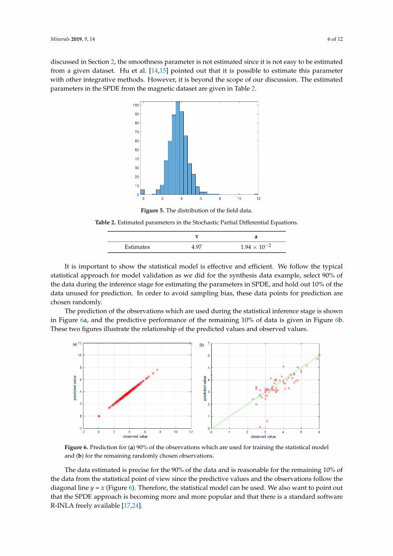
Here, we estimate the induced polarization field data with the SPDE model. Figure 5 shows thedistribution of the induced polarization field data, which follows the Gaussian distribution. As we

Minerals 2019, 9, 14 6 of 12

discussed in Section 2, the smoothness parameter is not estimated since it is not easy to be estimatedfrom a given dataset. Hu et al. [14,15] pointed out that it is possible to estimate this parameterwith other integrative methods. However, it is beyond the scope of our discussion. The estimatedparameters in the SPDE from the magnetic dataset are given in Table 2.

Minerals 2018, 8, x FOR PEER REVIEW 6 of 13

Here, we estimate the induced polarization field data with the SPDE model. Figure 5 shows the distribution of the induced polarization field data, which follows the Gaussian distribution. As we discussed in Section 2, the smoothness parameter is not estimated since it is not easy to be estimated from a given dataset. Hu et al. [14,15] pointed out that it is possible to estimate this parameter with other integrative methods. However, it is beyond the scope of our discussion. The estimated parameters in the SPDE from the magnetic dataset are given in Table 2.

Figure 5. The distribution of the field data.

Table 2. Estimated parameters in the Stochastic Partial Differential Equations.

τ a

Estimates 4.97 1.94 × 10−2

It is important to show the statistical model is effective and efficient. We follow the typical statistical approach for model validation as we did for the synthesis data example, select 90% of the data during the inference stage for estimating the parameters in SPDE, and hold out 10% of the data unused for prediction. In order to avoid sampling bias, these data points for prediction are chosen randomly.

The prediction of the observations which are used during the statistical inference stage is shown in Figure 6a, and the predictive performance of the remaining 10% of data is given in Figure 6b. These two figures illustrate the relationship of the predicted values and observed values.

The data estimated is precise for the 90% of the data and is reasonable for the remaining 10% of the data from the statistical point of view since the predictive values and the observations follow the diagonal line y = x (Figure 6). Therefore, the statistical model can be used. We also want to point out that the SPDE approach is becoming more and more popular and that there is a standard software R-INLA freely available [17,24].

Figure 7shows the prediction results of the induced polarization data. The contour map is plotted by the prediction field data. The data cover the full map and extend the area outside of the investigation field. A dense data matrix is expressed by the blue points located on the contour map. The high value of the induced polarization data is the interested area of the gold metallogenic prediction area. The warm color anomaly represents the high value of mine abnormality.

Figure 5. The distribution of the field data.

Table 2. Estimated parameters in the Stochastic Partial Differential Equations.

τ a

Estimates 4.97 1.94 × 10−2

It is important to show the statistical model is effective and efficient. We follow the typicalstatistical approach for model validation as we did for the synthesis data example, select 90% ofthe data during the inference stage for estimating the parameters in SPDE, and hold out 10% of thedata unused for prediction. In order to avoid sampling bias, these data points for prediction arechosen randomly.

The prediction of the observations which are used during the statistical inference stage is shownin Figure 6a, and the predictive performance of the remaining 10% of data is given in Figure 6b.These two figures illustrate the relationship of the predicted values and observed values.Minerals 2018, 8, x FOR PEER REVIEW 7 of 13

Figure 6. Prediction for (a) 90% of the observations which are used for training the statistical model and (b) for the remaining randomly chosen observations.

Figure 7. The SPDE prediction contour map of induced polarization data. The red and black symbols are the logging well with and without gold mine, respectively.

We mark three anomaly zones. Here, we take the IP1 anomaly zone as the example. The IP 1 anomaly zone location is fixed to the geological structure zone, which is presumed to be caused by the near-east-direction fault. The reason for the IP 1 anomaly zone is due to the carbonaceous rocks and metal sulfides around the fracture zone. Based on the regional situation of the ore field, the ore-control structure is the near-east–west direction. The shallow buried area is mainly quartz vein type gold deposit and fracture zone type gold deposit. Because the gold deposit is related to the carbonaceous material, metal sulfide, solicitation, etc., the IP 1 anomaly zone is of interest in future exploration work. We have drilled several wells for this exploration. In Figure 6, the red symbols are the wells with gold mines, such as ZK32601, ZK30401, ZK30403, ZK30701, and ZK30706. The blacks have not discovered the gold, which are ZK30802 and ZK30804.

Figure 6. Prediction for (a) 90% of the observations which are used for training the statistical modeland (b) for the remaining randomly chosen observations.

The data estimated is precise for the 90% of the data and is reasonable for the remaining 10% ofthe data from the statistical point of view since the predictive values and the observations follow thediagonal line y = x (Figure 6). Therefore, the statistical model can be used. We also want to point outthat the SPDE approach is becoming more and more popular and that there is a standard softwareR-INLA freely available [17,24].

Minerals 2019, 9, 14 7 of 12

Figure 7 shows the prediction results of the induced polarization data. The contour map is plottedby the prediction field data. The data cover the full map and extend the area outside of the investigationfield. A dense data matrix is expressed by the blue points located on the contour map. The highvalue of the induced polarization data is the interested area of the gold metallogenic prediction area.The warm color anomaly represents the high value of mine abnormality.

Minerals 2018, 8, x FOR PEER REVIEW 7 of 13

Figure 6. Prediction for (a) 90% of the observations which are used for training the statistical model and (b) for the remaining randomly chosen observations.

Figure 7. The SPDE prediction contour map of induced polarization data. The red and black symbols are the logging well with and without gold mine, respectively.

We mark three anomaly zones. Here, we take the IP1 anomaly zone as the example. The IP 1 anomaly zone location is fixed to the geological structure zone, which is presumed to be caused by the near-east-direction fault. The reason for the IP 1 anomaly zone is due to the carbonaceous rocks and metal sulfides around the fracture zone. Based on the regional situation of the ore field, the ore-control structure is the near-east–west direction. The shallow buried area is mainly quartz vein type gold deposit and fracture zone type gold deposit. Because the gold deposit is related to the carbonaceous material, metal sulfide, solicitation, etc., the IP 1 anomaly zone is of interest in future exploration work. We have drilled several wells for this exploration. In Figure 6, the red symbols are the wells with gold mines, such as ZK32601, ZK30401, ZK30403, ZK30701, and ZK30706. The blacks have not discovered the gold, which are ZK30802 and ZK30804.

Figure 7. The SPDE prediction contour map of induced polarization data. The red and black symbolsare the logging well with and without gold mine, respectively.

We mark three anomaly zones. Here, we take the IP1 anomaly zone as the example. The IP 1anomaly zone location is fixed to the geological structure zone, which is presumed to be caused by thenear-east-direction fault. The reason for the IP 1 anomaly zone is due to the carbonaceous rocks andmetal sulfides around the fracture zone. Based on the regional situation of the ore field, the ore-controlstructure is the near-east–west direction. The shallow buried area is mainly quartz vein type golddeposit and fracture zone type gold deposit. Because the gold deposit is related to the carbonaceousmaterial, metal sulfide, solicitation, etc., the IP 1 anomaly zone is of interest in future exploration work.We have drilled several wells for this exploration. In Figure 6, the red symbols are the wells with goldmines, such as ZK32601, ZK30401, ZK30403, ZK30701, and ZK30706. The blacks have not discoveredthe gold, which are ZK30802 and ZK30804.

4. Discussion

The field data is predicted by the SPDE model. The prediction method is also employed by theinterpolation method. We compare the common interpolation methods: for instance, the naturalneighbor interpolation [1,2], the nearest neighbor interpolation, the minimum curvature griddingmethod [5–7], and the Kriging method [3]. The same geophysical field data are employed to map thecontour in different interpolation method.

Figures show the interpolation contour map in natural neighbor interpolation (Figure 8),the nearest neighbor interpolation (Figure 9), the minimum curvature gridding method (Figure 10),and the Kriging interpolation method (Figure 11). The natural neighbor interpolation method predictsfield data that does not cover the full map. Only one anomaly is located at the northwesterninvestigation area. The result is similar to the minimum curvature and Kriging interpolation methods.All figures are not as smooth as the SPDE model contour map.

Minerals 2019, 9, 14 8 of 12

Minerals 2018, 8, x FOR PEER REVIEW 8 of 13

4. Discussion

The field data is predicted by the SPDE model. The prediction method is also employed by the interpolation method. We compare the common interpolation methods: for instance, the natural neighbor interpolation [1,2], the nearest neighbor interpolation, the minimum curvature gridding method [5–7], and the Kriging method [3]. The same geophysical field data are employed to map the contour in different interpolation method.

Figures show the interpolation contour map in natural neighbor interpolation (Figure 8), the nearest neighbor interpolation (Figure 9), the minimum curvature gridding method (Figure 10), and the Kriging interpolation method (Figure 11). The natural neighbor interpolation method predicts field data that does not cover the full map. Only one anomaly is located at the northwestern investigation area. The result is similar to the minimum curvature and Kriging interpolation methods. All figures are not as smooth as the SPDE model contour map.

Figure 8. The natural neighbor interpolation contour map. The red and black symbols are the logging well with and without gold mine, respectively.

Figure 9. The nearest neighbor interpolation contour map. The red and black symbols are the logging well with and without gold mine, respectively.

Figure 8. The natural neighbor interpolation contour map. The red and black symbols are the loggingwell with and without gold mine, respectively.

Minerals 2018, 8, x FOR PEER REVIEW 8 of 13

4. Discussion

The field data is predicted by the SPDE model. The prediction method is also employed by the interpolation method. We compare the common interpolation methods: for instance, the natural neighbor interpolation [1,2], the nearest neighbor interpolation, the minimum curvature gridding method [5–7], and the Kriging method [3]. The same geophysical field data are employed to map the contour in different interpolation method.

Figures show the interpolation contour map in natural neighbor interpolation (Figure 8), the nearest neighbor interpolation (Figure 9), the minimum curvature gridding method (Figure 10), and the Kriging interpolation method (Figure 11). The natural neighbor interpolation method predicts field data that does not cover the full map. Only one anomaly is located at the northwestern investigation area. The result is similar to the minimum curvature and Kriging interpolation methods. All figures are not as smooth as the SPDE model contour map.

Figure 8. The natural neighbor interpolation contour map. The red and black symbols are the logging well with and without gold mine, respectively.

Figure 9. The nearest neighbor interpolation contour map. The red and black symbols are the logging well with and without gold mine, respectively.

Figure 9. The nearest neighbor interpolation contour map. The red and black symbols are the loggingwell with and without gold mine, respectively.

Compared to these interpolation methods, the SPDE model-based prediction method can providenot only the contour map but also the uncertainty analysis. Our current implementation of the SPDEapproach is fast even without optimizing the code due to the Markov properties as pointed out byLindgren et al. [12]. Furthermore, the SPDE approach not only does the interpolation but also computesmany other quantities, such as the uncertainty of the prediction, the Hessian matrix of the parameters,and so on. These quantities are also useful for our future analysis. In order to illustrate this, we holdout 10% of our sample and use only 90% of the sample to estimate the parameters. This 10% of samplesare chosen randomly to avoid sampling bias, and this is a common practice in statistical analysis.The estimated parameters are used in the SPDE model to predict the remaining 10% as what wehave done in the synthetic example. The results are shown in Figure 12. From this figure, we cansee that the predicted data are near the observed data since the blue circles (predictions)are closeto the black crosses (observations). The prediction data are bounded by a 95% confidence interval,which are shown as red curves in Figure 12, and we can see that almost all the observations are insidethe confidence interval.

From the borehole data analysis, the anomaly IP1 has been separated into two parts. The lowerIP area (<3) in the IP1 area has been drilled by two wells: ZK30802 and ZK30804. Unfortunately, we

Minerals 2019, 9, 14 9 of 12

did not find any gold ore body or mineralization. In the Figures 6, 7 and 10, the SPDE, natural neighbor,and Kriging methods provided low IP anomalies. Compared to the natural neighbor and Kriging methods,the SPDE (Figure 6) showed more details. Because the owner only drilled in the IP1 area, the other twoanomalies IP2 and IP3 have not been verified by the drilling wells. Figure 13 shows the borehole resultsof the drilled seven wells in IP1 area. The deepest well, ZK30701, has been drilled 347.4 m.Minerals 2018, 8, x FOR PEER REVIEW 9 of 13

Figure 10. The minimum curvature interpolation contour map. The red and black symbols are the logging well with and without gold mine, respectively.

Figure 11. The Kriging interpolation contour map. The red and black symbols are the logging well with and without gold mine, respectively.

Compared to these interpolation methods, the SPDE model-based prediction method can provide not only the contour map but also the uncertainty analysis. Our current implementation of the SPDE approach is fast even without optimizing the code due to the Markov properties as pointed out by Lindgren et al. [12]. Furthermore, the SPDE approach not only does the interpolation but also computes many other quantities, such as the uncertainty of the prediction, the Hessian matrix of the parameters, and so on. These quantities are also useful for our future analysis. In order to illustrate this, we hold out 10% of our sample and use only 90% of the sample to estimate the parameters. This 10% of samples are chosen randomly to avoid sampling bias, and this is a common practice in statistical analysis. The estimated parameters are used in the SPDE model to predict the remaining 10% as what we have done in the synthetic example. The results are shown in Figure 12. From this figure, we can see that the predicted data are near the observed data since the blue circles (predictions)are close to the black crosses (observations). The prediction data are bounded by a 95% confidence interval, which are shown as red curves in Figure 12, and we can see that almost all the observations are inside the confidence interval.

From the borehole data analysis, the anomaly IP1 has been separated into two parts. The lower IP area (<3) in the IP1 area has been drilled by two wells: ZK30802 and ZK30804. Unfortunately, we did not find any gold ore body or mineralization. In the Figures 6, 7 and 10, the SPDE, natural

Figure 10. The minimum curvature interpolation contour map. The red and black symbols are thelogging well with and without gold mine, respectively.

Minerals 2018, 8, x FOR PEER REVIEW 9 of 13

Figure 10. The minimum curvature interpolation contour map. The red and black symbols are the logging well with and without gold mine, respectively.

Figure 11. The Kriging interpolation contour map. The red and black symbols are the logging well with and without gold mine, respectively.

Compared to these interpolation methods, the SPDE model-based prediction method can provide not only the contour map but also the uncertainty analysis. Our current implementation of the SPDE approach is fast even without optimizing the code due to the Markov properties as pointed out by Lindgren et al. [12]. Furthermore, the SPDE approach not only does the interpolation but also computes many other quantities, such as the uncertainty of the prediction, the Hessian matrix of the parameters, and so on. These quantities are also useful for our future analysis. In order to illustrate this, we hold out 10% of our sample and use only 90% of the sample to estimate the parameters. This 10% of samples are chosen randomly to avoid sampling bias, and this is a common practice in statistical analysis. The estimated parameters are used in the SPDE model to predict the remaining 10% as what we have done in the synthetic example. The results are shown in Figure 12. From this figure, we can see that the predicted data are near the observed data since the blue circles (predictions)are close to the black crosses (observations). The prediction data are bounded by a 95% confidence interval, which are shown as red curves in Figure 12, and we can see that almost all the observations are inside the confidence interval.

From the borehole data analysis, the anomaly IP1 has been separated into two parts. The lower IP area (<3) in the IP1 area has been drilled by two wells: ZK30802 and ZK30804. Unfortunately, we did not find any gold ore body or mineralization. In the Figures 6, 7 and 10, the SPDE, natural

Figure 11. The Kriging interpolation contour map. The red and black symbols are the logging wellwith and without gold mine, respectively.

Minerals 2018, 8, x FOR PEER REVIEW 10 of 13

neighbor, and Kriging methods provided low IP anomalies. Compared to the natural neighbor and Kriging methods, the SPDE (Figure 6) showed more details. Because the owner only drilled in the IP1 area, the other two anomalies IP2 and IP3 have not been verified by the drilling wells. Figure 13shows the borehole results of the drilled seven wells in IP1 area. The deepest well, ZK30701, has been drilled 347.4 m.

Figure 12. The uncertainty of the SPDE model-based prediction.

Figure 12. The uncertainty of the SPDE model-based prediction.

Minerals 2019, 9, 14 10 of 12Minerals 2018, 8, x FOR PEER REVIEW 11 of 13

Figure 13. Drilling well data. The red color illustrates the gold ore body, and the purple color illustrates the gold mineralization.

Figure 13. Drilling well data. The red color illustrates the gold ore body, and the purple color illustratesthe gold mineralization.

Minerals 2019, 9, 14 11 of 12

5. Conclusions and Future Work

The statistical model-based SPDE approach has been applied to predict the induced polarizationfield dataset. This approach constructs a statistical spatial model for geophysical dataset. Using thisapproach, the field data can be reconstructed and interpolated efficiently. The SPDE model can utilizethe information from the dataset and return precise delineation of IP anomalies. The reason is thatthe statistical model considers the relationship among different data locations, and the modeledrelationship fulfills the first law of geography which states “Everything is related to everything else,but near things are more related than distant things” [25]. The effectiveness and efficiency have beenapproved by the synthetic example. Then, we tested the method by a real field data case for the goldmineral exploration. The predicted values are quite close to the observed data. Compared to the naturalneighbor interpolation, the nearest neighbor interpolation, the minimum curvature interpolation, andKriging interpolation methods, the SPDE model-based method provided the smoothest and mostaccurate map. The borehole data have verified that the SPDE method gives more useful detailedinformation. The SPDE model-based method can provide the uncertainty of the prediction, and theuncertainty of the prediction is also obtained from the statistical model to help us in further research.In addition, we, in this paper, have fixed the value of parameter b. In practice, we can change thisparameter to control the smoothness, as discussed in Lindgren et al. [12], and we retain this part forour future work.

Currently, we only considered a simple SPDE in constructing the model. One direction of ourfuture work is to extend the statistical model to complex settings and to construct advanced statisticalmodels. Deeper statistical analysis can also be used, but this might go far beyond the scope of thispaper, and this is another direction of future work. In general, this approach might give us a new viewof how to use the available dataset, and we are trying to use and integrate the proposed method to beapplied in geology in the future.

Author Contributions: Conceptualization, Z.G. and X.H.; methodology, X.H.; software, X.H.; validation, Z.G.,X.H., and J.X.; formal analysis, Z.G. and X.H.; investigation, C.L.; data curation, C.L.; writing—original draftpreparation, Z.G. and X.H.; writing—review and editing, Z.G., X.H., and J.X.; visualization, J.L.; supervision, J.L.;funding acquisition, J.L., and J.X.

Funding: This research was funded by the National Natural Science Foundation of China grant number 41804073;41604080. The author has the financial support of The International Postdoctoral Exchange Fellowship Program.Project funded by China Postdoctoral Science Foundation grant number 2017M622607.

Acknowledgments: We thank the Longsheng Mining Co., Ltd. for allowing us to publish the results.We appreciate the jobs done by the colleagues on the data acquisition.

Conflicts of Interest: The authors declare no conflict of interest.

References

1. Sibson, R. A brief description of natural neighbor interpolation. In Interpreting Multivariate Data; Barnett, V.,Ed.; John Wiley: Chichester, UK, 1981; Chapter 2; pp. 21–36.

2. Watson, D. Contouring: A Guide to the Analysis and Display of Spatial Data; Elsevier: New York, NY, USA, 2013;Volume 10, ISBN 0080402860.

3. Cressie, N. The origins of kriging. Math. Geol. 1990, 22, 239–252. [CrossRef]4. Hansen, R. Interpretive gridding by anisotropic Kriging. Geophysics 1993, 58, 1491–1497. [CrossRef]5. Briggs, I.C. Machine contouring using minimum curvature. Geophysics 1974, 39, 39–48. [CrossRef]6. Swain, C.J. A FORTRAN IV program for interpolating irregularly spaced data using the difference equations

for minimum curvature. Comput. Geosci. 1976, 1, 231–240. [CrossRef]7. Webring, M. MINC: A Gridding Program Based on Minimum Curvature; Open-File Report; U.S. Geological

Survey: New York, NY, USA, 1981; pp. 81–1224.8. Claerbout, J.F. Multidimensional recursive filters via a helix. Geophysics 1998, 63, 1532–1541. [CrossRef]9. Claerbout, J.F.; Fomel, S. Image Estimation by Example: Geophysical Soundings Image Construction:

Multidimensional Autoregression; Stanford University: Stanford, CA, USA, 2008.

Minerals 2019, 9, 14 12 of 12

10. Guo, L.; Meng, X.; Shi, L. Gridding aeromagnetic data using inverse interpolation. Geophys. J. Int.2012, 189, 1353–1360. [CrossRef]

11. Kay, M.; Dimitrakopoulos, R. Integrated interpolation methods for geophysical data: Applications to mineralexploration. Nat. Resour. Res. 2000, 9, 53–64. [CrossRef]

12. Lindgren, F.; Rue, H.; Lindström, J. An explicit link between Gaussian fields and Gaussian Markov randomfields: The stochastic partial differential equation approach. J. R. Stat. Soc. 2011, 73, 423–498. [CrossRef]

13. Rue, H.; Held, L. Gaussian Markov Random Fields: Theory and Applications; CRC Press: Boca Raton, FL, USA, 2005.14. Hu, X.; Simpson, D.; Lindgren, F.; Rue, H. Multivariate Gaussian random fields using systems of stochastic

partial differential equations. arXiv, 2013; arXiv:1307.1379.15. Hu, X.; Lindgren, F.; Simpson, D.; Rue, H. Multivariate Gaussian random fields with oscillating covariance

functions using systems of stochastic partial differential equations. arXiv, 2013; arXiv:1307.1384.16. Hu, X.; Steinsland, I.; Simpson, D.; Martino, S.; Rue, H. Spatial modelling of temperature and humidity using

systems of stochastic partial differential equations. arXiv, 2013; arXiv:1307.1402.17. Lindgren, F.; Rue, H. Bayesian spatial modelling with R-INLA. J. Stat. Softw. 2015, 63, 1–25. [CrossRef]18. Hu, X.; Steinsland, I. Spatial modeling with system of stochastic partial differential equations.

Wiley Interdiscip. Rev. Comput. Stat. 2016, 8, 112–125. [CrossRef]19. Guo, Z.; Hu, X.; Dong, H. Model Based Interpolation for Magnetic Field Anomaly Analysis. In Proceedings

of the 75th EAGE Conference & Exhibition incorporating SPE EUROPEC, London, UK, 10–13 June 2013.20. Guo, Z.; Hu, X.; Liu, J. Modeling magnetic field data using Stochastic Partial Differential Equations.

In Proceedings of the Fourth international Conference on Engineering Geophysics Proceedings, Al Ain, UAE,9–12 October 2017.

21. Diggle, P.J.; Tawn, J.A.; Moyeed, R.A. Model based geostatistics. J. R. Stat. Soc. Ser. C Appl. Stat.1998, 47, 299–350. [CrossRef]

22. Cressie, N. Statistics for Spatial Data, Revised Edition. In Wiley Series in Probability and Mathematical Statistics;John Wiley & Sons, Inc.: Toronto, ON, Canada, 2015.

23. Stein, M.L. Interpolation of Spatial Data: Some Theory for Kriging; Springer Science & Business Media: NewYork, NY, USA, 2012.

24. Rue, H.; Riebler, A.; Sørbye, S.; Illian, J.; Simpson, D.; Lindgren, F. Bayesian computing with INLA: A review.Ann. Rev. Stat. Its Appl. 2017, 4, 395–421. [CrossRef]

25. Toler, W.R. A Computer Movie Simulating Urban Growth in the Detroit Region. Econ. Geogr. 1970, 2, 234–340.[CrossRef]

© 2018 by the authors. Licensee MDPI, Basel, Switzerland. This article is an open accessarticle distributed under the terms and conditions of the Creative Commons Attribution(CC BY) license (http://creativecommons.org/licenses/by/4.0/).