GEOMORPHIC AND STRUCTURAL EVOLUTION OF RELAY RAMPS DURING

NORMAL FAULT INTERACTION AND LINKAGE

AN ABSTRACT SUBMITTED ON THE THIRD DAY OF AUGUST, 2016 TO THE

DEPARTMENT OF EARTH AND ENVIRONMENTAL SCIENCES IN PARTIAL

FULFILLMENT OF THE REQUIREMENTS OF THE SCHOOL OF SCIENCE AND

ENGINEERING OF TULANE UNIVERSITY FOR THE DEGREE OF

DOCTOR OF PHILOSOPHY

BY

Michael C. Hopkins

APPROVED:

Nancye H. Dawers (Ph.D. Director)

_____________________________

Nicole M. Gasparini, Ph.D.

Brent M. Goehring, Ph.D.

_____________________________

Sean Bemis, Ph.D. (External Member)

ABSTRACT

Geomorphic features such as fluvial channels and shorelines can act as tape recorders of

accumulated tectonic deformation. Because these features can survive in a landscape for

up to105 years, the deformation represents tectonic activity over timescales longer than

earthquake cycles but shorter than geological timescales. Deformed landscape features

can be used to understand the impact of changing tectonic rates on landscape evolution

(given information on the tectonic processes involved). Conversely, we can take

advantage of how a landscape is expected to evolve and utilize those deviations to

explore details of tectonic processes that do not manifest over short timescales (i.e. single

earthquakes). Fault slip rate is expected to increase within the overlapping region of two

en echelon normal faults, but how increasing slip rate affects the landscape is poorly

understood (as discussed in Chapter 1). Additionally, details of this tectonic process that

occur over geomorphic timescales are not clearly understood. Chapter 2 of this

dissertation explores the impact of fault slip rate increase on fluvial channels during

normal fault interaction and linkage. Results of this work show that the landscape

responds by increasing channel slope and decreasing channel width before fault segments

link. Channel width only shows sustained decreases when a threshold channel slope of

about 0.05 is exceeded. In Chapter 3 vertically deformed lacustrine shorelines are

mapped along linked faults through the former overlap zones. These results show that

despite the presence of linking structures between faults, portions of the former

overlapping tips remain active post-linkage for 104 years. Chapter 4 investigates the

effect of fault length, spacing, and overlap on the area of relay ramps that drains parallel

to fault strike. Twenty-seven sites are examined and results show that for fault lengths

below 15 km most of the relay ramp area drains parallel to fault strike, whereas fault

lengths >15 km no particular drainage geometry is favored. Data on the overlap/spacing

ratio are biased to <2 for faults above ~15 km length. This bias is an inherent

characteristic because faults that define low overlap/spacing ratio relays do not link

rapidly and are, therefore, preserved within the landscape along large mature fault

systems. The results of this dissertation show that, while faults are mechanically

interacting, relay ramps are dynamic features that have significant impacts on landscape

evolution. Following complete linkage between segments, the relays do not behave as

passive structures and can actively deform over significant (>104 years) timescales.

Finally, the structural geometry of relay ramps impacts long-term morphodynamics and

channel network topology, which directly influences basin sedimentary architecture in

extensional basins.

GEOMORPHIC AND STRUCTURAL EVOLUTION OF RELAY RAMPS DURING

NORMAL FAULT INTERACTION AND LINKAGE

A DISSERTATION SUBMITTED ON THE THIRD DAY OF AUGUST, 2016 TO THE

DEPARTMENT OF EARTH AND ENVIRONMENTAL SCIENCES IN PARTIAL

FULFILLMENT OF THE REQUIREMENTS OF THE SCHOOL OF SCIENCE AND

ENGINEERING OF TULANE UNIVERSITY FOR THE DEGREE OF

DOCTOR OF PHILOSOPHY

BY

Michael C. Hopkins

APPROVED:

Nancye H. Dawers, Ph.D. (Director)

_____________________________

Nicole M. Gasparini, Ph.D.

Brent M. Goehring, Ph.D.

_____________________________

Sean Bemis, Ph.D. (External Member)

© Copyright by Michael C. Hopkins, 2016

All Rights Reserved

ii

ACKNOWLEDGMENTS

I would like to first acknowledge my adviser Nancye Dawers. I thank her for

supervising my dissertation research and for always being supportive during my Ph.D. I

thank my dissertation committee, Nicole Gasparini, Brent Goehring, and Sean Bemis for

their thoughtful comments and feedback. Reviewers Alexander Densmore, Alexander

Whittaker, Juliet Crider, Andrew Meigs, and one anonymous reviewer are thanked for

their comments, suggestions and feedback on the submitted manuscripts. Stacy Davies of

Roaring Springs Ranch, Frenchglen, OR, is thanked for giving access to ranch property to

make field observations for the work presented in Chapter 3.

Glenn Fisher, Heather Hoey, Jordan Adams and Matthew Dixon are thanked for

their assistance with field work and technical advice. I also want to thank all of the

friends I have made within the Department of Earth & Environmental Sciences at Tulane.

I could not have finished this work without them. Funding for this work was provided by

the American Chemical Society – Petroleum Research Fund (PRF-50833-ND8).

Summer support during part of this work was also provided by Schlumberger.

This dissertation is dedicated to my parents, Trudy A. Landry and Michael T.

Hopkins, for their unwavering support of my educational pursuits.

iii

TABLE OF CONTENTS

ACKNOWLEDGEMENTS……………………………………………………………….ii

LIST OF TABLES.....…………………………………………………………………….iv

LIST OF FIGURES……………………………………………………………………….v

CHAPTER

1. INTRODUCTION………………………………………………………………...1

2. CHANGES IN BEDROCK CHANNEL MORPHOLOGY DRIVEN BY

DISPLACEMENT RATE INCREASE DURING NORMAL FAULT

INTERACTION AND LINKAGE…..……………………………………………………9

3. VERTICAL DEFORMATION OF LACUSTRINE SHORELINES

ALONG BREACHED RELAY RAMPS, CATLOW VALLEY FAULT,

SOUTHEASTERN OREGON, USA………………………….…………………….......47

4. THE ROLE OF FAULT SCALE, SPACING AND OVERLAP IN

CONTROLLING RELAY RAMP CATCHMENT GEOMETRY……………………...80

Appendix

A. HEC-RAS MODELING……………………………………………................111

B. BASIN & RANGE SITE MAPS…....………………………………................117

BIBLIOGRAPHY………………………………………………………………………123

iv

LIST OF TABLES

4.1 Measurements and errors of fault length, overlap, spacing, ramp catchment area

and relay ramp area for study sites

A.1 HEC-RAS model parameters

v

LISIT OF FIGURES

1.1 Schematic block diagram of three faults illustrating the relay ramps, a schematic

map view of the Coulomb stress field following a slip event on a single fault and

displacement profiles of three faults illustrating their displacement patterns during fault

interaction

2.1 Schematic relay ramp diagram showing relay catchment and associated faults

2.2 Displacement profiles for two interacting normal faults

2.3 Study sites location map

2.4 Field photographs of fluvial channels

2.5 Unlinked and partially breached ramp 1 fault cut-off plots

2.6 Partially breached ramp 2 and fully breached ramp fault cut-off plots

2.7 Unlinked faults channel data

2.8 Partially breached ramp 1 and 2 channel data

2.9 Fully breached ramp channel data

2.10 Schmidt hammer data for channel knickpoints

2.11 Cartoon diagram illustrating fault displacement rate increase and accompanying

channel responses

3.1 Schematic block diagram of a linked pair of faults and the former relay ramp

3.2 Location map of Catlow Valley fault within the western Basin & Range

3.3 Locations of three breached relay ramps along Catlow Valley fault

3.4 Google Earth and field photograph of shorelines along the Catlow Valley

escarpment

vi

3.5 Block diagram illustrating shoreline terminology and maps illustrating how

shorelines were mapped

3.6 Shoreline map and elevation plots of shorelines along breached relay ramp ‘A’

3.7 Shoreline map and elevation plots of shorelines within ramp ‘A’

3.8 Shoreline map and elevation plots of shorelines along breached relay ramp ‘B’

3.9 Shoreline map and elevation plots of shorelines along breached relay ramp ‘C’

3.10 Google Earth imagery showing potential surface ruptures along Catlow Valley

fault and small faults within the upper portion of ramp ‘A’

3.11 Schematic line and block diagrams illustrating where deformation occurs on relay

breaching and adjacent structures following fault linkage

4.1 Block diagram illustrating relay ramp-parallel fluvial channels and ramp-

transverse channels

4.2 Study sites location map

4.3 Schematic block diagram and orthophoto of a relay ramp and associated

terminology

4.4 Orthophoto of normal fault tip mapped via GPS and remote sensing

4.5 Histograms of outboard fault length, spacing and overlap versus the number of

sites

4.6 Fault spacing versus overlap plot of this study and global dataset

4.7 Plot of outboard fault length versus down-ramp drained area (AFP) divided by

relay ramp area (AR)

4.8 Plot of outboard fault length versus fault overlap divided by fault spacing

vii

4.9 Schematic maps of scenarios by which relay fluvial systems may evolve as, or

transition, to a fault-transverse geometry

4.10 Google Earth images of scenarios depicted in Fig. 4.9

B1 Volcanic Tableland faults site maps

B2 Midway Hills faults site maps

B3 Palisade Mesa, Pearce and Buffalo Creek site maps

B4 Big Gulch, Blue Dome and Star Valley site maps

B5 Faults east of Abert Rim and Sheepshead Mountain fault site maps

B6 Catlow Valley and faults east of Summer Lake site maps

1

Chapter 1 Introduction

1.1 Motivation

Since the nineteenth century, understanding how landscapes evolve has been a

focus of geoscience research (Gilbert, 1877). One goal of geomorphological research is

to take a set of anomalous geomorphic observations in an actively deforming landscape

and tease out the tectonic processes that produced them (Burbank & Anderson, 2011).

Directly measuring tectonic processes is a time consuming, expensive, and highly site-

specific endeavor. One way to circumvent the challenge of directly measuring tectonic

processes is to utilize deformed landscape features (i.e., fluvial channels, terraces,

shorelines, etc.) to understand the tectonic perturbations that deformed the features.

Geomorphic features can act as a sort of tape recorder of the total accumulation of

tectonic deformation. Additionally, landscape features can record deformation over

timescales longer than a couple of earthquake cycles (103-10

5 years) and over large

spatial scales. With the advent of high-resolution elevation and imagery datasets, we can

make geomorphic observations readily and rapidly for large portions of Earth’s surface.

We can then utilize deviations in landscape form from what is expected in quiescent

environments to help tease out the tectonic perturbations that produced the anomalous

geomorphic signals over large swaths of Earth’s surface.

Over the last 25 years much attention has been given to understanding the

interplay between extensional tectonic geomorphology, normal fault evolution, and

stratigraphic architecture in rift basins (e.g., Gawthorpe & Hurst, 1993; Gawthorpe &

Leeder, 2000; Gupta et al., 1998; Dawers & Underhill, 2000; McLeod et al., 2002).

2

Normal fault growth has been well understood for several decades (e.g., Peacock &

Sanderson, 1991; Dawers et al., 1993; Cartwright et al., 1995, 1996; Childs et al., 1995;

Willemse, 1997; Cowie, 1998; Gupta & Scholz, 2000; Cowie & Roberts, 2001). More

recently, however, workers have sought to understand the impact extensional tectonics

has on an array of geomorphological processes and features such as fluvial incision

(Commins et al., 2005; Whittaker et al., 2007a, b, 2008; Kirby & Whipple, 2012)

drainage pattern and catchment evolution (Densmore et al., 2004; Cowie et al., 2006) and

scarp facet morphology (Topal et al., 2016). These studies are particularly useful

because they take advantage of a well-understood tectonic process and show how the

landscape responds. Interactions between geomorphological and tectonic processes

directly impact sedimentary transport and deposition, and therefore directly influence

both temporal and spatial patterns of synrift stratigraphy.

The over-arching goal of this dissertation is two-fold. Firstly, I take advantage of

a well-understood tectonic process - specifically the evolution of normal faults via fault

segment interaction and linkage - and investigate the impact this has on a landscape.

Secondly, I utilize geomorphic features to draw a clearer picture of extensional tectonic

processes on timescales longer than an earthquake cycle but shorter than geological

timescales. It is vital to have a clear picture of the influence of fault evolution (both

spatial and temporal) on geomorphological processes to fully realize the development of

stratigraphic sequences in extensional basins, many of which comprise important

hydrocarbon provinces.

3

1.2 Approach

Many insights into the structural and geomorphic evolution of normal faults can

be gleaned by focusing on so-called relay ramps. Relay ramps are structural features

between overlapping normal fault segments (Larsen, 1988) (Fig. 1.1a).

Relay ramps can provide sediment transport pathways from the eroding footwall block of

a fault array into the adjacent basin (Gawthorpe & Hurst, 1993; Gupta et al., 1999; Cowie

Fig. 1.1: (a) Block diagram of relay ramps along overlapping normal faults. (b) Map view of a single Andersonian normal fault with an illustration of how the surrounding Coulomb stress field changes following a slip event (Modified from Hodgkinson et al., 1996 & Cowie, 1998). (c) Map view and displacement profiles of three faults showing how zones of positive stress change affect displacement profiles and displacement rates on neighboring faults.

4

et al., 2006). Areas where faults overlap are generally topographically lower than the rest

of the fault array. Sediment transport systems can, therefore, exploit these lows and

utilize them as entry points into the hanging wall basin. When normal faults are in an

overlapping en echelon geometry they interact with one another such that they mutually

increase each other’s slip rate. When a single normal fault slips, stress in the surrounding

rock volume is reduced in some locations and increased in others (Fig. 1.1b). If a

segment is oriented such that a zone of positive stress change overlaps a neighboring

fault, slip on that segment makes slip more likely to occur on the neighbor (Fig. 1.1c)

(Cowie, 1998). Stress loading and reloading between neighboring faults initiates a

positive feedback, which ultimately increases the slip rate on portions of the overlapping

segments. Increases in slip rate, in this manner, lead to asymmetrical displacement

profiles with maxima that are skewed towards the overlap zone (Peacock & Sanderson,

1991; Willemse et al., 1996) (Fig. 1.1c).

The well-studied and predictable pattern of fault growth via segment interaction

and linkage provides a useful framework within which to study the geomorphological

response to faulting. Furthermore, by examining processes across of range of scales, we

can substitute space for time and use small fault arrays as the framework for

understanding the early landscape evolution in rifted terrains and large crustal scale fault

arrays for more mature tectonic landscapes. For example, studying the response of

fluvial channels that flow down relay ramps along small faults can provide insight into

the patterns of fluvial incision that reflect the landscape’s early evolution. Intermediate

length fault arrays provide insights into more evolved faults that are likely to have linked

segments, but may still be in the stage of localizing deformation on relay breaching

5

faults, which should have a signature in the landscape. Long fault arrays with large

segments, large total displacement and high slip rate exhibit footwall drainage catchments

that may vary in size and shape as parameters such as segment overlap and spacing

change. The research presented in this dissertation was carried out in order to address all

these issues.

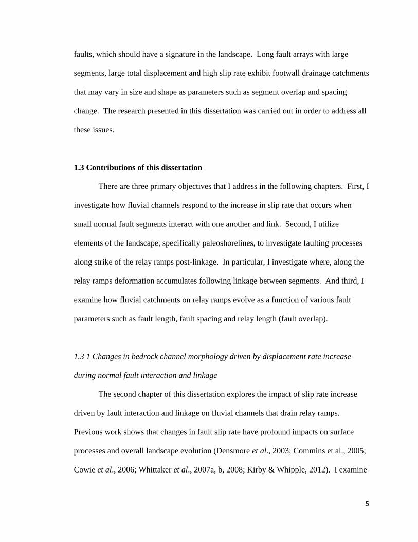
1.3 Contributions of this dissertation

There are three primary objectives that I address in the following chapters. First, I

investigate how fluvial channels respond to the increase in slip rate that occurs when

small normal fault segments interact with one another and link. Second, I utilize

elements of the landscape, specifically paleoshorelines, to investigate faulting processes

along strike of the relay ramps post-linkage. In particular, I investigate where, along the

relay ramps deformation accumulates following linkage between segments. And third, I

examine how fluvial catchments on relay ramps evolve as a function of various fault

parameters such as fault length, fault spacing and relay length (fault overlap).

1.3 1 Changes in bedrock channel morphology driven by displacement rate increase

during normal fault interaction and linkage

The second chapter of this dissertation explores the impact of slip rate increase

driven by fault interaction and linkage on fluvial channels that drain relay ramps.

Previous work shows that changes in fault slip rate have profound impacts on surface

processes and overall landscape evolution (Densmore et al., 2003; Commins et al., 2005;

Cowie et al., 2006; Whittaker et al., 2007a, b, 2008; Kirby & Whipple, 2012). I examine

6

four relay ramp sites in this chapter; the faults associated with each ramp are overall

small, immature, and in various stages of interaction and linkage. The sites include an

unlinked pair of faults, two ramps that may or may not be partially breached by a linking

structure and one site where the overlapping faults are fully linked. I collected channel

slope and cross-sections with a GPS receiver along the length of the channels at each site.

In addition, I measured fault throw along the faults that border the relay ramps. Because

these channels are not active, I used the cross-sectional data to model flow with HEC-

RAS, a one-dimensional open channel flow model, to extract measurements of channel

width, water depth, and bed shear stress. The results show that the channels at three of

these sites display distinct geomorphological responses to the increase in slip rate

associated with fault interaction and linkage. Specifically, the channels are steeper and

narrower when clear indications of fault interaction (indicated by the asymmetrical

displacement profiles, Fig. 1.1c) are present. Moreover these geomorphological

responses are present when evidence that the faults are in the process of linking is

ambiguous.

1.3.2 Vertical deformation of lacustrine shorelines along breached relay ramps, Catlow

Valley fault, southeastern Oregon, USA

The third chapter of this dissertation investigates the structural evolution of relay

ramps, focusing on the timescale over which relay-bounding fault tips remain active post-

fault linkage. The ultimate fate of a relay ramp (i.e., whether it simply subsides into the

basin post-fault linkage or actively deforms post-linkage) influences sediment transport

systems that traverse the ramp. As such, it is crucial to fully understand what structural

7

processes might influence these systems. Previous work implies that, following fault

linkage, the former fault tips become inactive (Peacock & Sanderson, 1991; Cartwright et

al., 1996; Cowie, 1998). Analog models suggest, however, that the fault tips of the

former segments remain active post-linkage (Hus et al., 2005), but it has not been

documented in nature. In this chapter I map well-preserved late Pleistocene lacustrine

paleoshorelines along three fully breached relay ramps within the Catlow Valley fault

system in southeastern Oregon. Paleoshorelines are horizontal datums that can give

indications of where fault displacement has accumulated along strike of the linked fault

segments. Results show that shoreline elevations deviate from average shoreline

elevation along strike of the relay ramps. These results also show that fault slip has not

localized on the linking structures, despite the presence of fully formed linking faults.

This observation demonstrates that relays are subject to active deformation following

complete fault linkage for up to 104 years. The implication is that fluvial systems can

still be affected by this deformation and can considerably influence sediment transport

pathways and depocenter locations in early synrift basins.

1.3.3 The role of fault scale, overlap and spacing in controlling extensional relay ramp

fluvial system geometry

The fourth and final chapter of this dissertation examines both the structural and

geomorphic characteristics on the evolution of fluvial catchments that drain relay ramp

surfaces, across a wide spectrum of spatial and temporal scales. In Chapter 2, the fluvial

systems that drain the ramps are oriented such that flow is parallel to fault strike.

Previous work suggests this is typical and is what to be expected in nature (Gawthorpe &

8

Hurst, 1993, Gupta et al., 1999); however, numerous examples exist where this is not the

case (Jackson & Leeder, 1994; Densmore et al., 2003; Athmer & Luthi, 2011; Duffy et

al., 2015). Instead of flowing parallel to fault strike, some relay channels flow across the

outboard fault scarp and bypass the ramp altogether (Fig. 1a). The purpose of this

chapter is to examine what structural parameters are associated with particular relay ramp

fluvial geometry. Twenty-seven sites are examined in the Basin and Range (including

sites discussed in Chapters 2 and 3), and the parameters measured are relay ramp area,

area of the relay ramp that drains parallel to fault strike, outboard fault length, ramp

width (i.e., fault spacing) and length (i.e., fault overlap). The results show that at

outboard fault lengths of less than ~15-20 km, a majority of the relay ramp area drains in

the direction that is parallel to fault strike. At fault lengths greater than ~20 km, there is

no association between fault length and fluvial geometry. High overlap/spacing ratios are

associated with relays along shorter (< 20 km long) outboard faults, whereas lower

overlap/spacing ratios are associated with relays along longer faults. Overlap/spacing

ratio and fault scale relationships suggest that lower overlap/spacing ratio relays may be

more common along longer outboard faults because they survive for longer periods of

time in the landscape.

9

Chapter 2

Changes in bedrock channel morphology driven by displacement rate increase

during normal fault interaction and linkage

This chapter was published in Basin Research.

HOPKINS, M.C. & DAWERS, N.H. (2015) Changes in bedrock channel morphology driven

by displacement rate increase during normal fault interaction and linkage. Basin

Research, 27, 43-59. doi: 10.1111/bre.12072.

2.1 Abstract

We attribute changes in the morphology of relay ramp channels (increased slope

and decreased width) to variations in displacement rate on ramp-adjacent normal faults.

We map the faults and fluvial channels associated with four sites in different stages of

fault interaction and linkage on the Volcanic Tableland, a middle Pleistocene ash-flow

tuff in east central California. Because these channels are inactive today, we estimate

downstream changes in channel width and depth using HEC-RAS, a one-dimensional

open channel flow model. Our results show that channel slope must be greater than about

0.05 before there are substantial decreases in width or substantial increases in depth.

Displacement rate increases during interaction between en echelon segments results in

the increases in channel slope and decreases in channel width. Moreover, our data show

that these changes begin to occur during the very early stages of fault interaction, well

before the fault geometry would indicate ongoing or imminent linkage.

10

2.2 Introduction

Changes in fluvial channel morphology have been widely used to infer changes in

rock uplift rate (Duvall et al., 2004), changes in fault activity (Commins et al., 2005;

Whittaker et al., 2007a, b, 2008; Kirby & Whipple, 2012), and to predict the evolution of

fluvial systems in response to fault interaction and linkage (Densmore et al., 2003; Cowie

et al., 2006). Fluvial channels that flow down relay ramps, i.e., the region between

overlapping normal fault segments, are highly sensitive to displacement rate changes and

deformation associated with fault interaction and linkage (Fig. 2.1).

Because relay ramps occur across an evolutionary spectrum, from simple fault overlaps

to deformed ramps that are breached by linking faults, they offer unique opportunities to

investigate patterns of bedrock channel incision, including progressive changes in

Fig. 2.1. Schematic block diagram of a relay ramp, adjacent faults and a fluvial channel that drains the relay ramp.

11

channel slope and width. Relay ramps are especially useful because temporal and spatial

changes in the rock uplift field occur in predictable ways. Our aim here is to examine a

set of small fluvial channels on relay ramps associated with normal fault segments in

different stages of fault interaction and linkage, located on the Volcanic Tableland of

northern Owens Valley in eastern California, USA. We describe the manner in which the

longitudinal profiles and channel widths evolve through various stages of relay

development, by placing these observations within the framework of fault array and relay

ramp evolution. The ultimate goal here is to examine changes in bedrock channel

morphology by using the temporal framework defined by the fault array evolution.

2.2.1 Rationale for this study & expected transient channel responses

The rationale for this study is that, by combining bedrock channel data with fault

displacement data from field sites in different stages of fault interaction and linkage, we

will be able to examine the bedrock channel response to increased slip rate associated

with fault evolution. We can take advantage of anomalies in the fault displacement

profiles to determine the degree of interaction between segments when evidence of a

definitive linking structure is lacking. Using the fault array and relay geometry as a

proxy for time facilitates comparison between channel morphology that is slightly

perturbed by faulting versus channel morphology that is strongly affected by fault

interaction and linkage.

Because of the increase in cumulative fault displacement across each stage of

relay evolution, we anticipate that increases in channel slope associated with the

increasing tilt of the ramp, and base level change associated with fault slip events, should

12

drive progressive incision of the channels. Understanding the controls on channel width

in bedrock channels remains an active area of research in geomorphology (Whipple,

2004; Finnegan et al., 2005; Wobus et al., 2006; Turowski et al., 2006; 2007). One

outstanding issue is how width adjusts when a channel experiences differential rock uplift

(e.g., Amos & Burbank, 2007; Yanites & Tucker, 2010). Examining relay ramp channels

in different stages of fault interaction and linkage allows us to substitute these stages as a

proxy for time, and examine how channel slope and width changes through time.

Commins et al. (2005), utilized bedrock channels to constrain the timing of the

displacement rate increase and found that channel morphology was affected enhanced

displacement rates. We take this a step further and examine the detailed channel

morphology changes to understand the fluvial response to fault interaction and linkage.

Such integrated studies of channel response and the faulting process have been, thus far,

under-utilized (Kirby & Whipple, 2012).

2.2.2 Using fault array and relay geometry as a proxy for time

Normal faults typically grow by the linking of en echelon segments to form larger

faults (e.g., Cartwright et al., 1995; Dawers & Anders, 1995). Cowie (1998) showed that

the en echelon geometry arises from patterns of stress change associated with fault slip.

Moreover, if en echelon faults are in an optimal geometry where zones of positive stress

change overlap, a positive feedback develops where slip on one fault reloads its neighbor,

making it more likely to fail (Cowie, 1998). Ultimately, this causes displacement rates to

increase on both fault segments (Fig. 2.2). This has been observed in both numerical

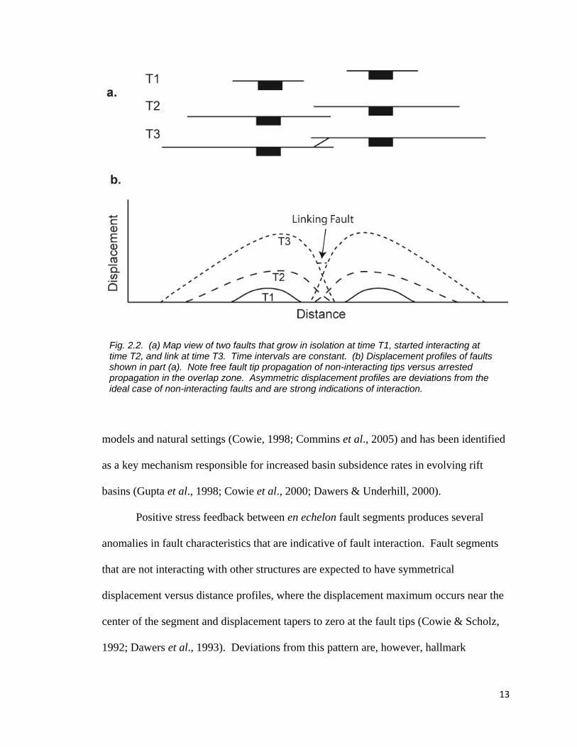
13

models and natural settings (Cowie, 1998; Commins et al., 2005) and has been identified

as a key mechanism responsible for increased basin subsidence rates in evolving rift

basins (Gupta et al., 1998; Cowie et al., 2000; Dawers & Underhill, 2000).

Positive stress feedback between en echelon fault segments produces several

anomalies in fault characteristics that are indicative of fault interaction. Fault segments

that are not interacting with other structures are expected to have symmetrical

displacement versus distance profiles, where the displacement maximum occurs near the

center of the segment and displacement tapers to zero at the fault tips (Cowie & Scholz,

1992; Dawers et al., 1993). Deviations from this pattern are, however, hallmark

Fig. 2.2. (a) Map view of two faults that grow in isolation at time T1, started interacting at time T2, and link at time T3. Time intervals are constant. (b) Displacement profiles of faults shown in part (a). Note free fault tip propagation of non-interacting tips versus arrested propagation in the overlap zone. Asymmetric displacement profiles are deviations from the ideal case of non-interacting faults and are strong indications of interaction.

14

indications of fault interaction (Willemse et al., 1996); these include asymmetrical

displacement profiles and steep displacement gradients on overlapping fault tips (Fig.

2.2).

Relay ramps are also recorders of the fault array evolution. As the segments

evolve, the ramps are initially little-deformed, but as displacement accrues and

displacement gradients on the interacting overlapping faults become steeper, the ramps

tend to tilt more steeply toward the mutual hanging wall (Peacock & Sanderson, 1991)

and slip events occur more frequently (Cowie, 1998). In addition, fault splays and small

faults begin to partially breach the ramp. At a later stage, a linking fault will transect the

relay, physically linking to the two segments (Peacock & Sanderson, 1991; Trudgill &

Cartwright, 1994).

Taken together, the nature of the relay ramps and the characteristics of fault

displacement patterns along the adjacent normal faults provide a temporal framework

within which to unravel patterns of bedrock channel evolution. In other words, relay

channel sites can be identified in terms of three developmental stages: a channel draining

a simple fault overlap with limited evidence of fault interaction, a channel on a partially

breached relay ramp that exhibits, for example, steep displacement gradients on the

overlapping faults, and finally a scenario in which a relay channel has clearly been

perturbed by a linking fault developed fully across the relay ramp.

2.3 Geological Setting

The study area is located in northern Owens Valley in east-central California, at

the western margin of the Basin and Range province. Owens Valley is a transtensional

15

basin located within the Eastern California Shear Zone (ECSZ), a zone of dextral shear

originating from differential motion of the Pacific plate relative to the North American

plate (Dokka & Travis, 1990a). Since 6-10 Ma, the ECSZ has accommodated

approximately 25% of the strike-slip motion along the plate boundary (Dokka & Travis,

1990b; Miller et al., 2001; Dixon et al., 2003).

Northern Owens Valley is, in part, defined by the Volcanic Tableland, which is

composed of the welded portion of the Upper Pleistocene Bishop Tuff. Emplacement of

the Bishop Tuff took place ca. 758.9 +/- 1.8 ka, as a result of a voluminous pyroclastic

eruption from Long Valley Caldera (Sarna-Wojcicki et al., 2000), located north-

northwest of the Tableland. The Bishop Tuff is a welded rhyolitic tuff and is roughly 150

meters thick on average (Gilbert, 1938). Lithologically, the Bishop Tuff is relativity

uniform but stratigraphic distinctions can be made on the degree of welding, types of

lithic fragments, and chemical variations in pumice and air fall deposits (Gilbert, 1938;

Bateman, 1965; Wilson & Hildreth, 1997).

The Tableland surface is characterized by joints and fumarole mounds, which are

abundant and probably formed soon after emplacement, a population of north-south

striking normal faults and an inactive stream network. The fault network and fluvial

channels formed since emplacement of the tuff and represent the deformational and

erosional history of the Tableland over the last ~760,000 years (Gilbert, 1938; Bateman,

1965; Pinter, 1995; Pinter & Keller, 1995). The channel patterns in plan-view show that

the stream network formed as a result of the evolving fault population geometry; trellis

patterns are evident and some channels are sourced from uplifted footwalls (Bateman,

16

1965; Pinter & Keller, 1995; Gilpin, 2003). Thus the area offers a unique opportunity for

investigating fault interaction and linkage and its impact on the landscape.

Most Tableland faults appear to be purely extensional, though some strike-slip

motion may be accommodated by the en echelon arrangement of some segments

(Bateman, 1965; Pinter, 1995); the individual fault segments we examine in this study

exhibit only normal slip. Because of relatively limited erosion across the upper surface

of the Tuff (Goethals et al., 2009), scarp height is a proxy for cumulative fault

displacement (Bateman, 1965, Dawers et al., 1993; Dawers & Anders, 1995; Pinter,

1995; Ferrill et al., 1999). The area of the Tableland examined in this study consists of

mostly en echelon arrangements of fault segments, with each segment being less than ~2

km in length (Fig. 2.3).

Most of the faults in the array discussed here dip to the west; however a few small

faults within the array are antithetic. The timing of fault initiation on the Volcanic

Tableland is unknown. While no historical surface rupturing earthquakes have originated

from a Tableland fault, surface fractures developed near some Tableland faults during the

1986 Chalfant Valley earthquake sequence (Lienkaemper et al., 1987). Some faults

within the population were active in the latest Pleistocene as evidenced by offset fluvial

terraces of the Owens River near the southern edge of the Tableland (Pinter et al., 1994).

The Tableland’s channels tend to be relatively small, with most being only a few meters

wide and less than 1 m deep (Fig. 2.4). These channels appear to have been created by

fluvial processes due to the abundance of features such as flutes, potholes, and plunge

pools. Channel flow appears to have followed the regional depositional slope of the ash-

flow sheet from northwest to southeast (Bateman, 1965; Pinter & Keller, 1995), but as

17

they interacted with the evolving fault population many channels were diverted by local

fault-related topography and channelized flow also developed on relay ramps.

Fig. 2.3. 1:12,000 Digital Orthophoto Quarter Quadrangle (DOQQ) showing field sites examined in this study, courtesy of the U.S. Geological Survey. The DOQQ is the northwest part of the Fish Slough 7.5’ (1:24,000) Quadrangle, Inyo County, California. Channel location and flow direction indicated by lines with arrows. Tick marks are on downthrown side of faults. Latitude and longitude of eastern and northern boundaries are noted.

18

The channels discussed here flow down relay ramps, and were locally sourced from the

fault array’s footwall and were mapped only to the base of the relay ramp.

The channels are not presently active but they are thought to have been active

several times since emplacement of the Bishop Tuff. The pre-Tahoe and Tahoe

glaciations are two time periods when the channels were likely active (Pinter & Keller,

1995); however this has not been definitively shown. Gilpin (2003) obtained cosmogenic

26Al and

10Be dates on a relay channel system just west of the sites studied here and

concluded that channel occupation dates from ~70 ka to ~300 ka. Though the history of

channel occupation is not completely known, what is important to our study is that the

Fig. 2.4. Photographs of Tableland bedrock channels. (a) ~ 1 m high relay ramp knickpoint, (b) imbricated clasts. Locations are noted in Fig. 2.3.

19

channel incision is coeval with Tableland fault evolution, and that channel morphology

here is driven by local faulting (Bateman, 1965; Pinter & Keller, 1995; Gilpin, 2003).

Subsequent to channel abandonment, we do not see evidence of widespread channel

modification by blanketing of aeolian deposits. Furthermore, our observations suggest

that hillslope processes have probably not significantly modified Tableland channels

subsequent to abandonment. We reach this conclusion based on the fact that the current

climate is dry, slopes are relatively low across the Tableland, and primary channel

features are preserved.

While we acknowledge the fact that the channel geometry can be modified by

fault displacement while the channels are inactive, what is important to note here is that

our primary interest is in the relative states of channel deformation. Because each site we

have chosen represents a discrete point in time relative to fault interaction and linkage,

we are only investigating the relative deformation associated with each stage. For

example, if we examine two sites in which one is clearly at a more advanced stage of

interaction/nearing linkage, we would expect the channel to be more deformed (i.e.,

higher slopes) due to increases in displacement rate. Although channel deformation may

very well occur while the channels are inactive, we expect deformation during these

inactive periods will be partitioned in such a way that channels on ramps at advanced

stages of interaction/linkage have experienced more deformation than ramps in earlier

stages. Furthermore, we see no evidence for post-abandonment activity within any of the

channels. We do not observe any vertical offset of fluvially abraded rock surfaces within

any channel at a location where we have interpreted a linking fault. This observation

20

suggests that post-abandonment surface rupturing fault activity on the linking structures

has not occurred.

2.4 Methods

Within our study area, we mapped the faults and fluvial channels associated with

four field sites, including one pair of unlinked en echelon faults and three relay ramps,

two of which are partially breached by a linking fault and one that is fully breached (Fig.

2.3). We chose these sites because they offer the opportunity to investigate the evolving

fault geometry and channel response across a temporal spectrum from unlinked to

completely linked faults. In addition, we focused on channels having similarly sized

drainage areas, which are given on Fig. 2.3. The drainage areas represent the total area

drained by each catchment upstream of its outlet and were calculated using a combination

10 m DEM and GPS points obtained in the field.

2.4.1 Field data

We mapped the faults and channels using a Trimble GeoXH-2008-3000 Series

handheld GPS receiver connected to an external antenna that is capable of 10 cm post-

processing vertical accuracy. Faults adjacent to each field site were mapped by walking

the crest and base of the fault scarps (i.e., the footwall and hanging wall cutoffs, see Fig.

2.1) through the fault relay zone. Channels were mapped along the thalweg, moving

upstream until geological evidence of channelized flow (e.g., evidence of thalweg or

channel banks) could no longer be discerned. We define our study channels as ‘bedrock’

if rock outcrops in the channel banks and bed or if channel cover is only a veneer. We

21

surveyed channel cross-sections perpendicular to the flow direction, at a spacing that

varies from about 10 to 100 m. Where channel morphology changes rapidly, we used

smaller cross-section spacing and used larger spacing where channel morphology

displays little variation.

Fault cutoff plots were generated by projecting field data points onto a line that

best represents average fault strike, as determined from aerial photographs. The average

strike of each fault was found by mapping it on aerial photographs using ESRI’s ArcGIS

software. We then found the slope-intercept form of the strike line by using UTM

northing and easting coordinates as ‘x’ and ‘y’ Cartesian coordinates. Because the

shortest distance between the strike line and any point along the cutoffs is a straight line,

we know the slope of that line is perpendicular to the mapped strike line. We can then

define the equation of a line that goes through any data point and the strike line. With

two equations we algebraically solved for the intersection of two lines; the coordinate

pair (expressed in UTM) is used as the projected coordinates. By projecting the cutoffs

onto an average fault strike, errors in the throw gradient that are associated with the

collection process (because they were not collected in a straight line) are reduced. The

result is a realistic visualization of the cutoff geometry. We generated fault throw plots

by subtracting the elevation of data points on the hanging wall cutoff from the elevation

of data points on the footwall cutoff, provided both points are within 1 m of each other

laterally. Error in fault throw plots should not be significant at 1 m increments.

Channel longitudinal profiles and channel slope were plotted directly from the

field data. Profiles were generated by plotting the elevation associated with each data

point and accumulating the straight-line distance between them. Profiles reflect channel

22

length because the channels do not meander and the data coverage is dense enough to

capture true channel length. Slope plots are 200 m running averages of slope calculated

in the upstream direction. Because we wanted to retain as much slope data from the

upstream and downstream ends of the channels as possible, while at the same time reduce

noise, we chose a 200 m window. By choosing at 200 m window, we reduced noise (i.e.,

larger windows did not significantly alter the slope plots) and we retained as much data

as possible.

To account for the possibility of lithological variation, we measured rock

competence with a Schmidt hammer. Rock strength should not vary much because all of

our sites are entirely within the Bishop Tuff, but knickpoints could be generated because

of local lithological variability related to degree of welding. We collected 15 Schmidt

hammer measurements from both the upstream and downstream sides of 7 knickpoints

and calculate the mean, maximum and minimum rebound values. Measurements were

collected on horizontal surfaces with the Schmidt hammer held vertically above the rock

surface. Care was taken to avoid measurements adjacent to joints and we only took

measurements on intact bedrock surfaces.

2.4.2 HEC-RAS models

In order to examine how channel morphology changes in the Tableland channels

we must have some way of objectively examining morphology that is free of

interpretation bias. Because the fluvial channels on the Tableland are no longer active,

we cannot directly measure channel width and depth, so we use HEC-RAS v.4.1.0, a

freely available one-dimensional open channel flow model developed by the U.S. Army

23

Corps of Engineers. We use HEC-RAS to model flow in our study channels and extract

measurements of depth, width and bed shear stress under different flow regimes and

discharge scenarios. We define depth here as the maximum water depth in the active

channel, width as the water width at the top of the flow, and shear stress as the product of

the unit weight of water, hydraulic radius and energy slope (U.S. Army Corps of

Engineers, Hydrological Engineering Center). Here, slope used by HEC-RAS is

calculated from the cross-section elevations. The advantage of HEC-RAS for this study

is that it offers an opportunity to unambiguously extract channel width and depth. It is

difficult to use our field data alone to define channel width and depth, especially because

the channels are not active. After processing the GPS data we imported channel cross-

sections into the model and set the necessary flow parameters. All cross-sections were

entered into HEC-RAS by inputting the distance and elevation associated with each GPS

point collected in each cross-section. Next, the lateral distance between each cross-

section is entered. To perform the flow models, HEC-RAS requires discharge,

Manning’s ‘n’, boundary conditions, a flow regime, and coefficients of fluid expansion

and contraction. For more details on HEC-RAS model equations, parameters used, and

data collection see Appendix A.

Once the channel geometry and flow parameters were selected we ran two flow

models for each channel: one at half-discharge and one at full-discharge (discharge does

not change downstream for each model, see Appendix A for full discussion). Full-

discharge is the largest amount of water that can be contained within all the cross-

sections associated with each channel. Half-discharge is simply half of the full discharge.

Values of width, depth and bed shear stress from both model runs are averaged between

24

the two runs and plotted. On Figs. 2.7, 2.8, and 2.9 the plotted lines show the average

values of width, depth, and bed shear stress and the bars show the range between full and

half discharge. We chose this method because it allows us to see where the modeled flow

is responding to changes in channel morphology rather than discharge.

2.4.3 Reference width

In order to make an assessment of how width changes in our study channels, we

include a reference width in Figs. 2.7, 2.8 & 2.9, which we obtained by using the width-

area scaling relationship. In the width-area relationship W = kAx, ‘W’ is channel width,

‘k’ is some coefficient, ‘A’ is drainage area, and ‘x’ is some power ranging from 0.3-0.5

(Hack, 1957; Whipple, 2004; Whittaker et al., 2007a). Although we make the

simplifying assumption that discharge is not changing downstream (which would mean

we hold drainage area ‘A’ in the width-area scaling relationship constant for a given site)

it is, nonetheless, instructive to have a reference with which to see how channel geometry

changes from what would be ‘expected’. To determine the reference width, we first set

‘x’ to 0.5 (see Whittaker et al., 2007a) and find the value of ‘k’ that best fits the width-

area relation for the unlinked faults channel. We plot the reference width line on the

same graph as the HEC-RAS model width and adjust the ‘k’ value until the difference

between the average model width and reference width is the smallest. We then take the

coefficient that results in the best match between the model and reference width and

apply it to the other three sites. Even though slope does increase in the downstream

direction for some portion of the channel reach at the unlinked faults, it has a negligible

influence on width. The average width of the channel where slope decreases downstream

25

is 5.61 m and with the addition of width measurements where slope increases

downstream, average width is 5.64 m. We took this approach because the unlinked faults

site is the most representative of quiescence.

2.5 Results

2.5.1 Fault data

For each fault we describe the general fault geometry, asymmetry in both cutoff

geometry and throw profiles, and the maxima. Upper plots in Figs. 2.5 and 2.6 illustrate

cutoff geometry of major ramp bounding faults and lower plots show throw versus

distance profiles for each fault.

2.5.1.1 Unlinked faults

The unlinked faults consist of two en echelon faults without evidence of a linking

fault (Fig. 2.5a-c). Based on the cutoff plots (Fig. 2.5b), the upper part of this ramp tilts

towards the inboard fault and the ramp as a whole has a fairly constant slope towards the

south. Note that there are two local maxima on the inboard fault displacement profile

(Fig. 2.5c), which suggests the inboard fault is actually composed of two linked, nearly

co-planar, segments. Throw maxima on the inboard and outboard faults do not exceed 15

m.

2.5.1.2 Partially breached ramp 1

The fault geometry at partially breached ramp 1 is more complex than at the

unlinked faults site. There are two primary faults, i.e., the inboard and outboard

segments, and two smaller faults (fault splays) that bifurcate from the outboard fault. A

noticeable change in strike of the outboard fault toward the inboard fault is an indication

26

that the faults are in the process of linking, so we call this relay ramp ‘partially’ breached.

Fig. 2.5. Fault cutoffs and throw profiles for the unlinked faults and faults near partially breached ramp 1. (a & d) Map view of relay ramps, their associated faults, and the channels that drain the relays, (b & e) projected fault cutoffs, (c & f) throw profiles. Note the slight inboard fault asymmetry and off centered throw maximum associated with inboard fault in ‘c’. Note that the inboard fault throw profile ‘f’ at partially breached ramp 1 is highly asymmetrical (the inboard fault is the continuation of outboard fault in Fig. 6d). Cumulative throw is shown for fault splays. Throw profile asymmetry with off-centered throw maxima are indications of fault interaction, therefore the unlinked faults are interacting but not linked; faults at partially breached ramp 1 are interpreted to be in the process of linking.

27

Cutoff data and the throw profiles show a highly asymmetric inboard fault (Fig. 2.5e &

f). The ramp tilts, in general, towards the inboard fault over its entire length. The slope

of the ramp towards the south is fairly constant from 0 to 500 m on the ‘x’ axis (Fig.

2.5e) but does increase slightly from 600-750 m. The throw maxima on these faults are

35 m on the outboard fault, ~60 m on the inboard fault and ~20 m on the fault splays

(note that only cumulative throw of the splays is shown).

2.5.1.3 Partially breached ramp 2

The cutoff plot (Fig. 2.6b) shows that the inboard fault is actually two faults that

are linked; however the throw profile (Fig. 2.6c) resembles that of a single fault, so we

show cumulative throw only. We apply the term partially breached here because of the

presence of a nascent linking fault, but the fault has not completely breached the ramp.

This ramp does not tilt toward either the inboard or outboard fault and the slope towards

the south is essentially constant. The faults associated with partially breached ramp 2

have throw maxima of ~35 m on the outboard fault, ~25 m on the inboard fault, and < 15

m on the breaching fault.

2.5.1.4 Fully breached ramp

At the site of the fully breached ramp, the inboard and outboard faults are clearly

linked by a single fault (fault labeled linking fault Fig. 2.6d). The outboard fault throw

profile is highly asymmetric (Fig. 2.6e); note that this fault is the continuation of the

inboard fault in Fig. 2.5e. The inboard fault throw profile here is slightly asymmetric

(Fig. 2.6f). The ramp does not consistently tilt toward either the inboard or outboard fault

and the slope of the ramp toward the hanging wall (south) is fairly uniform. Throw

28

maxima are ~45 m on the outboard fault, ~20 m on the inboard fault and < 10 m on the

linking fault.

29

2.5.2 Channel Data

2.5.2.1 Unlinked faults

The channel bed is predominantly alluvial with bedrock outcrops only at the

channel head and mouth. The channel profile at this site (Fig. 2.7a) contains a minor

convex reach ~250 m upstream of the channel mouth (see Figs. 2.5 and 2.6 for maps of

all channel planforms). The running average of channel slope is highest at the channel

outlet and decreases in the upstream direction to 500 m upstream of the mouth. In

general, slope increases from 500 m upstream of the outlet to the channel head (Fig.

2.7b). Channel width varies by about 3 m along the length of the channel, and the

channel contains two areas between 0 and 750 m upstream of the channel mouth where

width narrows below the reference width (Fig. 2.7c). Depth fluctuates considerably

through most of the channel reach but, moving upstream from the channel mouth, depth

does show an unambiguous decrease around 250 m and 750 m. (Fig. 2.7d). Bed shear

stress is less than 30 N/m2 (Fig. 2.7e) and shows no clear change in association with

changes in either depth or width. The only feature that bed shear stress appears to have

any correlation with is the increase in slope from 250-0 m upstream of the channel

mouth.

Fig. 2.6. Fault cutoff and throw profiles for partially breached ramp 2 and the fully breached ramp. (a & d) Map view of relay ramps, their associated faults and the channels that drain the relays, (b & e) projected fault cutoffs. (c & f) Throw profiles of faults associated with fully breached ramp. Faults at partially breached ramp 2 are interpreted to be at a more advanced stage of linkage than partially breached ramp 1 because of the presence of a fault that nearly breaches the entire relay ramp. The data gap in the throw profile on the outboard fault is due to a breaching fault. Note that the outboard fault here is a continuation of the inboard fault in Fig. 2.5f. Inboard and outboard faults are fully linked. Data gaps (solid lines) along the outboard fault throw profile of both ‘c’ and ‘f’ are related to breaching faults.

30

Fig. 2.7. Field data and HEC-RAS model results for the channel at the unlinked faults site. (a) Longitudinal. (b) 200 m running average of channel slope. (c) Channel width. (d) Depth. (e) Bed shear stress. A minor convex reach near the channel mouth is related to the incorporation of a small fault (see Fig. 5c). Slope decreases from a maximum of ~ 0.03 at the channel mouth to below 0.02 about 500 m upstream of the channel mouth. Moving upstream, slope increases through the rest of the channel reach. Trends in width, depth and bed shear stress do not consistently follow increase in slope.

31

2.5.2.2 Partially breached ramp 1

The channel profile at partially breached ramp 1 shows a prominent convex reach

from ~400 to ~750 m upstream of the channel mouth (Fig. 2.8a). Moving upstream, the

running average of channel slope dramatically increases at the downstream end of the

fault overlap zone and reaches a maximum of value of 0.09 about 500 m upstream of the

channel mouth (Fig. 2.8b). Channel width varies by ~4 m through the channel reach

(Fig. 2.8c). Substantial changes in width are noted from 0 to ~100 m upstream of the

channel mouth; however, these variations are not associated with any significant changes

in the profile or slope. Just downstream of the fault overlap zone, width narrows ~ 4 m

below the reference width and remains 3-4 m narrower than the reference width until

~750 m upstream of the channel mouth. Although width increases upstream of 750 m

above the channel mouth by 1-3 m, some width measurements are below the reference

width. Water depth fluctuates by about 0.15 m through the channel reach. There are

definite increases in depth associated with slope values above ~0.05 and width values

below the reference width (Fig. 2.8d). One large increase in depth associated with a

notable decease in slope is noted ~100 m upstream of the channel mouth. Bed shear

stress varies from ~10 to ~100 N/m2 and reaches a maximum near the maximum values

of slope and minimum width values (Fig. 2.8e). Bed shear stress increases through the

channel from 0 to ~400 m upstream of the channel mouth and, in general, decreases

upstream.

2.5.2.3 Partially breached ramp 2

Two profile convexities are evident in the channel profile from partially breached

ramp 2; one convexity is located about 300 m upstream of the channel mouth and the

32

33

second is located about 600 m upstream of the channel mouth (Fig. 2.8f). The

downstream convexity is located at the breaching fault (Fig. 2.8f). Although the fault

does not intersect the channel at the surface (its tip is located about only about 10 m

away) it is likely present at depth. The running average of slope reaches a maximum

value of ~0.08 in the downstream convex reach. The upstream convex reach also shows

elevated slope values, but they are not as high as in the downstream convex reach. In

general, most measurements of channel width fall below the reference width (Fig. 2.8h).

Channel width is highly variable at this site but two features are noteworthy. The lowest

width measurements fall ~4 m below the reference width in the vicinity of the highest

slope values. Channel width also falls below the reference width in the vicinity of the

second convex reach by 1-4 m. There are places where width varies significantly both

above and below the reference width, but it is worth mentioning that lower widths are

only sustained through the downstream convex reach. Upstream about 1000 m from the

channel mouth, width is highly variable both above and below the reference width.

Similar to width, depth is also highly variable (Fig. 2.8i). In general, depth appears to

decrease in the upstream direction. Shear stress is highly variable but higher values (>75

Fig. 2.8. Field data and HEC-RAS model results for channel at partially breached ramp 1 (a-e) and partially breached ramp 2 (f-j). (a) Longitudinal profile of channel at partially breached ramp 1. (b) 200 m running average of channel slope. (c) Channel width. (d) Depth. (e) Bed shear stress. (f) Longitudinal profile of channel at partially breached ramp 2. (g) 200 m running average of channel slope. (h) Channel width. (i) Depth. (j) Bed shear stress. Profile and slope plots for partially breached ramp 1 (a & b) show one broad convex reach with maximum slopes approaching 0.09, associated with substantial decreases in width below the reference width, increases in depth, and increases in bed shear stress. Profile and slope data for partially breached ramp 2 (f & g) show two convex reaches. The downstream convex reach has slope values approaching 0.08 and is associated with sustained decreases in width, increases in depth, and increases in shear stress. While decreases in width, increases in depth and increases in shear stress are noted through the upstream convex reach (slope maximum approaching 0.05) they are not as substantial, nor are they sustained.

34

N/m2) are noted in the vicinity of the two convex reaches (Fig. 2.8j). The highest shear

stress value (~175 N/m2) is associated with the linking fault.

2.5.2.4 Fully breached ramp

One profile convexity is present and is coincident with the linking fault in the

fully breached ramp (Fig. 2.9a). Two peaks in the running average of slope are obvious

(Fig. 2.9b): one is associated with the linking fault and the other, which is the highest

slope observed in this channel, is located within 100 m of the channel head. The slope

plot in Fig. 2.9b is noticeably different from Fig. 2.8b & g, in that there are two

‘plateaux’ (~400-600 m upstream of the channel mouth) in the slope profile of Fig. 2.9b.

Slope, in general, increases from the channel mouth and reaches a value of ~0.065 just

downstream of the linking fault. We attribute the decrease in in slope here to be related

to backtilting of the footwall of the linking fault. Moving in the upstream direction from

the linking fault, slope decreases then increases again to reach a maximum of ~0.075.

Most width measurements upstream of ~250 m above the channel mouth fall below the

reference width by 0.5-5 m. Decreases in width below the reference width in this channel

are associated with increases in slope. Water depth (Fig. 2.9d) shows a general decrease

in the upstream direction, but it is highly variable. Width also decreases below the

reference width through what we term ‘bedrock ridges’. Here, the channel is paralleled

on either side by elevated linear ridges of bedrock. There appears to be an association

between the bedrock ridges and lower width values. The ridges may represent a local

lithological variation within the Bishop Tuff because they are not laterally extensive, but

we cannot say for certain why these ridges exist. Shear stress is highly variable and

appears to increase from 0 to 400 m upstream of the channel mouth then seems to

35

Fig. 2.9. Field data and HEC-RAS model results for channel at fully breached ramp. (a) Longitudinal profile, (b) 200 m running average of channel slope. (c) Channel width. (d) Depth. (e) Bed shear stress. Profile and slope data (a & b) show a distinct convexity associated with the linking fault. Width, depth and shear stress do not appear to follow trends in slope. Except for distinct geometric changes associated with channel confinement due to the bedrock ridges (see text), elevated slope values alone do not appear to be associated with decreases in width below the reference width, increases in water depth, or increases in shear stress.

36

fluctuate, but the highest shear stress measurements are associated with the steepest

slopes and lowest width measurements (Fig. 2.9e).

2.5.3 Schmidt Hammer Data

We collected 210 Schmidt hammer rebound measurements on the downstream

and upstream sides of seven knickpoints in channels on partially breached ramp 1 and 2.

Figure 2.10 shows the maximum, mean and minimum values for rebound measurements.

There appears to be no difference (p = 0.06) in mean Schmidt hammer rebound values on

the downstream and upstream side of knickpoints (Fig. 2.10).

2.6 Interpretations

Our results indicate that channel morphology is substantially affected by

displacement rate increase during fault interaction and linkage. During the very earliest

stages of interaction, for example partially breached ramp 1, channel morphology appears

to respond by increasing slope, decreasing width, and increasing depth. Though we

Fig. 2.10. Mean, maximum and minimum rebound values of 210 Schmidt hammer measurements on the upstream and downstream sides of seven knickpoints. The knickpoints are located in channels at partially breached ramp 1 and 2.

37

interpret morphological changes in our study channels to be driven by displacement rate

increase, we also discuss the potential impact that climate fluctuations and lithological

variability have on our results. We do not attribute these changes to a manifestation of

progressive surface deformation of the ramp surface. We reach this conclusion because

changes in cutoff gradients, which are the best information we have on the three

dimensional orientation of the ramp surfaces, do not correlate with changes in channel

morphology.

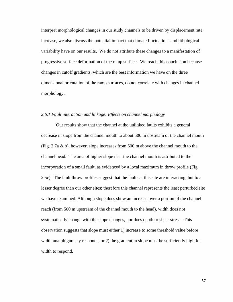
2.6.1 Fault interaction and linkage: Effects on channel morphology

Our results show that the channel at the unlinked faults exhibits a general

decrease in slope from the channel mouth to about 500 m upstream of the channel mouth

(Fig. 2.7a & b), however, slope increases from 500 m above the channel mouth to the

channel head. The area of higher slope near the channel mouth is attributed to the

incorporation of a small fault, as evidenced by a local maximum in throw profile (Fig.

2.5c). The fault throw profiles suggest that the faults at this site are interacting, but to a

lesser degree than our other sites; therefore this channel represents the least perturbed site

we have examined. Although slope does show an increase over a portion of the channel

reach (from 500 m upstream of the channel mouth to the head), width does not

systematically change with the slope changes, nor does depth or shear stress. This

observation suggests that slope must either 1) increase to some threshold value before

width unambiguously responds, or 2) the gradient in slope must be sufficiently high for

width to respond.

38

Our data on the channel morphology at partially breached ramp 1 show that slope

increases and reaches a maximum within the fault overlap zone (Fig. 2.8a). In addition,

width decreases, depth increases just downstream of the steepened reach, and shear stress

increases through the steepened portion of the channel (Figs. 2.8c-e). The fault throw

profiles show significant asymmetry indicating that the faults are interacting more

strongly than the unlinked en echelon faults (Fig. 2.5f) and may, in fact, be close to

linking. The peaks in slope and shear stress in this channel are spatially coincident with

maximum throw on the fault splays, and the region of increasing slope occurs over the

length of the splays. The perturbation in this channel is probably not related directly to

interaction between the inboard and outboard fault segments. We interpret the channel

perturbation to be related to the presence of the fault splays. It is not entirely clear

whether the fault splays are the future site of linkage between the inboard and outboard

segments. The presence and growth of the fault splays are probably heavily influenced

by interaction between the inboard and outboard fault, as evidenced by steep throw

gradients on the splays and a high throw maximum relative to the inboard and outboard

segments.

We observe two convex reaches in the channel at partially breached ramp 2. The

presence of a linking fault (see Fig. 2.6a) indicates that the faults at this site are at a later

stage of linkage than either the unlinked en echelon faults or partially breach ramp 1.

While two areas of elevated slope are noted in this channel, width, depth and shear stress

do not show a consistent response. If we examine the downstream area of elevated slope

we observe an unmistakable decrease in width (4 m below the reference width) a subtle

increase in depth and an increase in shear stress (Fig. 2.8g). However, if we examine the

39

upstream convex reach, decreases in width are not so clear-cut. While there are decreases

in width, they are not, overall, as substantial as the downstream convex reach, nor do all

width measurements fall below the reference width. This ambiguous response is

similarly noted in depth measurements. While shear stress does show a substantial

increase in the upstream convex reach, elevated shear stress values are not sustained

through this reach as they are in the downstream convex reach. These observations

suggest that there may be a threshold slope value beyond which there is an unmistakable

response. If we compare the results of partially breached ramp 1 and 2, both show that a

threshold slope value of ~0.05 is required before width and depth show a clear, persistent

response.

In the case of the fully breached relay, we see no evidence of channel profile

convexities except for the one clearly related to the linking fault; however, width and

depth are highly variable. Additionally, the highest slope values in the channel appear to

be confined to the upstream half of the channel (Fig. 2.9b). Based on the presence of a

completely through-going linking fault, we interpret this site to be the most advanced, in

terms of the fault evolution, of all the sites we examined. Because the fully breached

ramp has already experienced the increase in displacement rate associated with the onset

of fault interaction, this channel probably had the most time to adjust to the imposed

perturbation. In the same vein as our interpretations for the partially breached cases, we

expect that where slope is >0.05, width, depth and shear stress should show a clear

response (i.e., narrowing, deepening, and increasing respectively). However, there is not

a sharp response. Although there are clearly elevated slope values above 0.05, there are

not sustained decreases in width, increases in depth or increases in shear stress. The only

40

area where there are distinct and sustained decreases in width are where the channel is

flanked by the bedrock ridges. While elevated slope values are coincident with changes

in width, depth and shear stress, it appears that elevated values in both slope and the

gradient of slope may actually be important in causing spatially sustained and

unambiguous changes in channel geometry. In every case we examined, our data clearly

show that sustained changes in width, depth and shear stress, are associated with slope

values that must be above about 0.05 and that the gradient of slope must be sufficiently

high (see partially breached ramp 1 and 2 slope plots Fig. 2.8b/g for comparison to Fig.

2.9b).

Clearly, the values of width, depth and bed shear stress may not reflect the actual

values when these channels were active in the past. Nevertheless, the trends contained

within the HEC-RAS modeled data make physical sense. This is supported by Fig. 2.8

and 2.9 that show prominent convexities in the longitudinal profiles and field evidence of

channel confinement (i.e., bedrock ridges), where we expect width to decrease, depth to

increase and bed shear stress to increase.

2.6.2 Lithology and climate

We acknowledge that convexities in the longitudinal profile of a channel may be

generated by a number of factors including base level lowering due to other factors (i.e.,

climate induced base level lowering) or lithological variation (Phillips & Lutz, 2008). In

this section we discuss the effects lithology and climate have on our study. While we do

not see evidence suggesting lithological variation or climate-driven base level lowering

are important factors here, we do not wish to dismiss them outright.

41

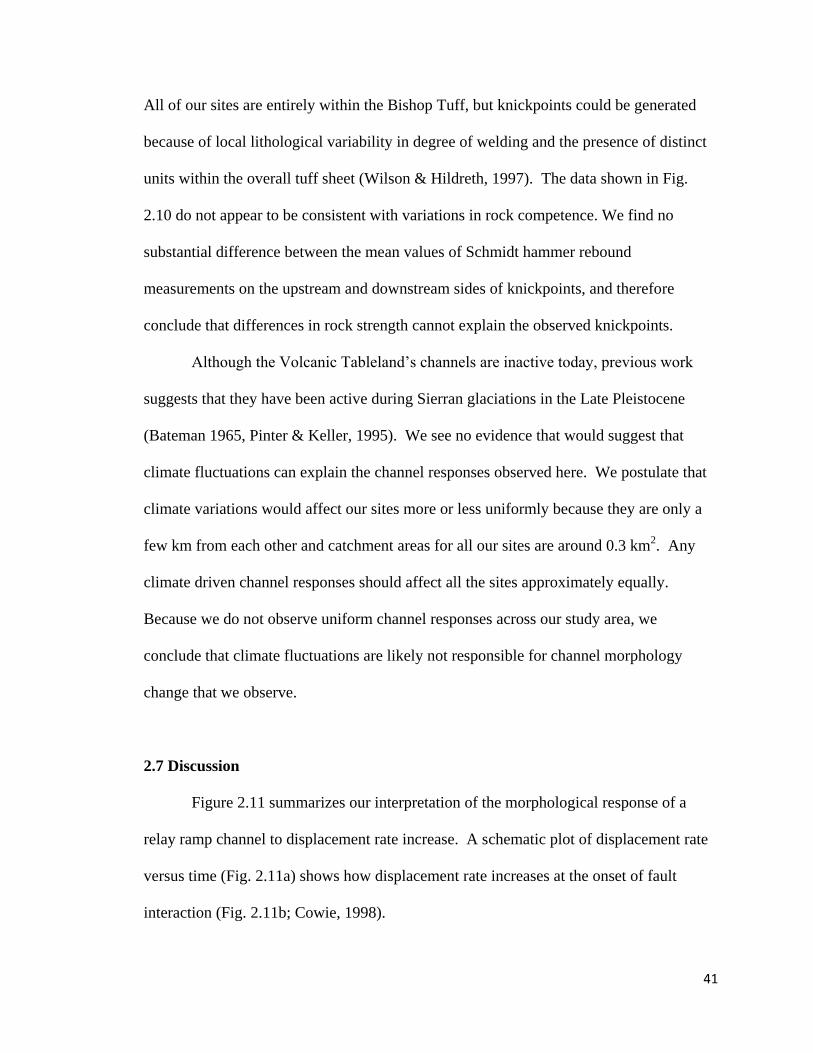
All of our sites are entirely within the Bishop Tuff, but knickpoints could be generated

because of local lithological variability in degree of welding and the presence of distinct

units within the overall tuff sheet (Wilson & Hildreth, 1997). The data shown in Fig.

2.10 do not appear to be consistent with variations in rock competence. We find no

substantial difference between the mean values of Schmidt hammer rebound

measurements on the upstream and downstream sides of knickpoints, and therefore

conclude that differences in rock strength cannot explain the observed knickpoints.

Although the Volcanic Tableland’s channels are inactive today, previous work

suggests that they have been active during Sierran glaciations in the Late Pleistocene

(Bateman 1965, Pinter & Keller, 1995). We see no evidence that would suggest that

climate fluctuations can explain the channel responses observed here. We postulate that

climate variations would affect our sites more or less uniformly because they are only a

few km from each other and catchment areas for all our sites are around 0.3 km2. Any

climate driven channel responses should affect all the sites approximately equally.

Because we do not observe uniform channel responses across our study area, we

conclude that climate fluctuations are likely not responsible for channel morphology

change that we observe.

2.7 Discussion

Figure 2.11 summarizes our interpretation of the morphological response of a

relay ramp channel to displacement rate increase. A schematic plot of displacement rate

versus time (Fig. 2.11a) shows how displacement rate increases at the onset of fault

interaction (Fig. 2.11b; Cowie, 1998).

42

The onset of fault interaction causes the channel profile, initially at equilibrium, to

deform (Fig. 2.11c) and as this interaction continues, channel deformation continues.

Following physical linkage, the channel profile regains a concave up form (except for the

convexity at the linking fault), but width and depth are still highly variable.

Fig. 2.11. Schematic cartoon showing the morphological evolution of a Tableland relay ramp channel. (a) Plot showing displacement rate before and after the onset of fault interaction. (b) Displacement vs. distance plots and schematic map of non-interacting fault segments and interacting fault segments. (c) Idealized channel slope and width plots illustrating how we interpret a relay ramp channel to respond to displacement rate increase associated with fault interaction. Pre-Interaction: Assumed equilibrium or near equilibrium conditions, predicted width assumes some width-drainage area relationship (i.e., W α A

x,

see text). During fault interaction slope responds to enhanced displacement rate by increasing within the overlap zone; compare with data in Fig. 2.8b & g. Our data show that width shows a clear and sustained response only in conjunction with slopes above ~0.05.

43

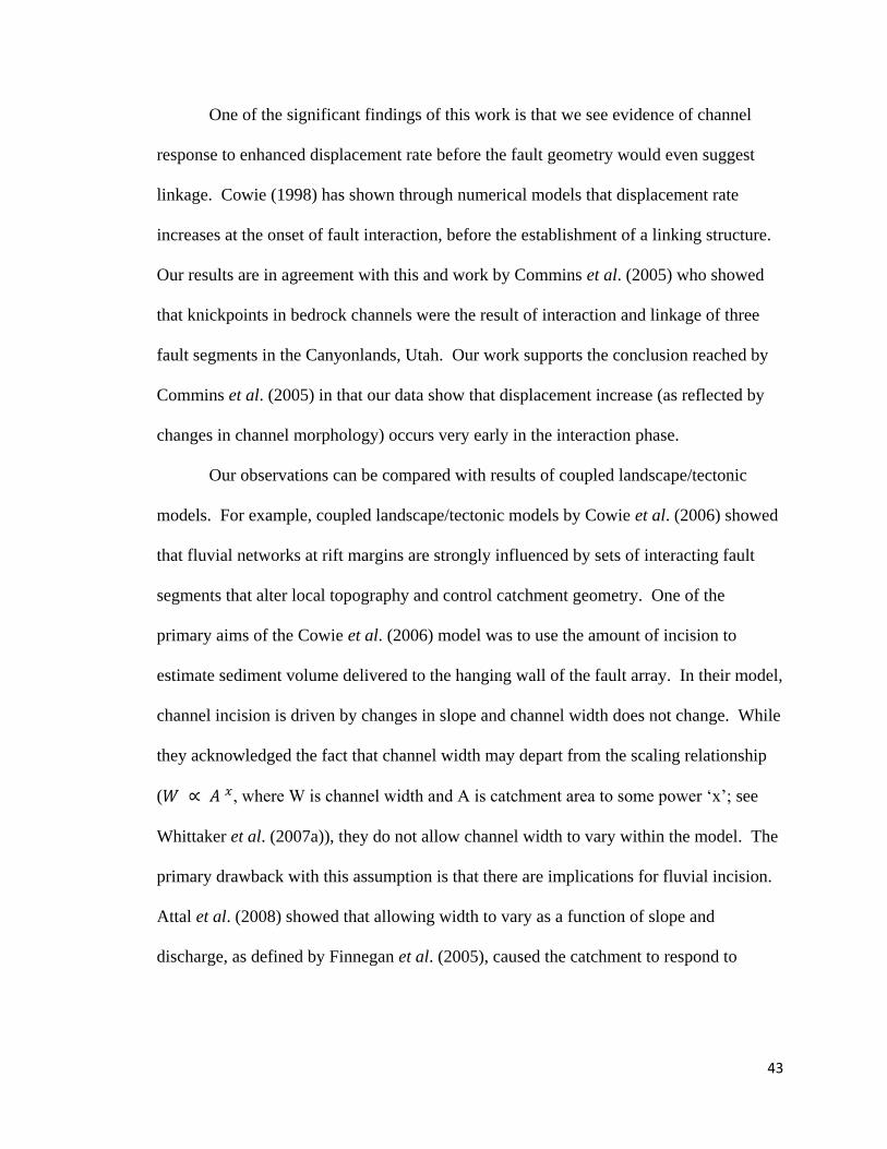
One of the significant findings of this work is that we see evidence of channel

response to enhanced displacement rate before the fault geometry would even suggest

linkage. Cowie (1998) has shown through numerical models that displacement rate

increases at the onset of fault interaction, before the establishment of a linking structure.

Our results are in agreement with this and work by Commins et al. (2005) who showed

that knickpoints in bedrock channels were the result of interaction and linkage of three

fault segments in the Canyonlands, Utah. Our work supports the conclusion reached by

Commins et al. (2005) in that our data show that displacement increase (as reflected by

changes in channel morphology) occurs very early in the interaction phase.

Our observations can be compared with results of coupled landscape/tectonic

models. For example, coupled landscape/tectonic models by Cowie et al. (2006) showed

that fluvial networks at rift margins are strongly influenced by sets of interacting fault

segments that alter local topography and control catchment geometry. One of the

primary aims of the Cowie et al. (2006) model was to use the amount of incision to

estimate sediment volume delivered to the hanging wall of the fault array. In their model,

channel incision is driven by changes in slope and channel width does not change. While

they acknowledged the fact that channel width may depart from the scaling relationship

(𝑊 ∝ 𝐴 𝑥, where W is channel width and A is catchment area to some power ‘x’; see

Whittaker et al. (2007a)), they do not allow channel width to vary within the model. The

primary drawback with this assumption is that there are implications for fluvial incision.

Attal et al. (2008) showed that allowing width to vary as a function of slope and

discharge, as defined by Finnegan et al. (2005), caused the catchment to respond to

44

changes in tectonic activity more rapidly than if width were tied to discharge (or drainage

area) alone.

Our results show that width and depth in channels near interacting fault segments

appear to show sustained decreases and increases, respectively, only when slope is above

about 0.05. This notion implies that bedrock channels may only show unambiguous

responses to differential rock uplift once a high enough gradient has been imparted on the

channel flowing across the uplift. The notion of a threshold is not new. Previous work

has suggested that, at relatively low uplift rates channel morphology can be insensitive to

change due to a threshold effect (Turowski et al., 2007). On the other hand, the existence

of this threshold means that at more rapid tectonic rates, information may be gleaned

about the tectonic uplift field in areas where transient slope perturbations are no longer

preserved, but narrowed channel reaches remain. Amos and Burbank (2007) observed

that fluvial channels narrowed in response to transient perturbations in the slope profile

generated by differential uplift. The channel slopes Amos and Burbank (2007) observed

were less than half of the 0.05 slope threshold that we observe on the Volcanic Tableland.

This discrepancy, however, makes physical sense because their channels were of

comparable size, but bedrock (our study) is more difficult for a channel to incise into than

alluvium (Amos and Burbank, 2007) and would, therefore, require higher slopes. The

magnitude of the observed slope threshold is no doubt highly site specific in that channel

size, bed cover, discharge and bedrock type will affect channel incision and, therefore,

would necessitate a different threshold slope.

The results discussed here have implications for studies that model relay ramp

catchment evolution along fault systems at crustal scales. One issue that remains poorly

45

understood in these systems is when relay catchments (such as the ones we study here)

transition from watersheds where the bulk of water and sediment is directed toward the

base of the ramp to those that bypass the ramp. Densmore et al. (2003) modeled relay

catchment evolution and concluded that competition between fault array evolution and

catchment erosion exerted a fundamental control on the evolution of the catchments.

Densmore et al. (2003) interpreted that headward erosion of catchments on the outboard

fault scarp controls whether relay catchments are ultimately captured. We suggest that

displacement rate increase is a plausible mechanism that can explain their observation. If

displacement rate increase causes the relay channel system to incise faster than

catchments on the outboard fault scarp can erode, then the relay drainage area will remain

relativity intact.

2.8 Conclusions

Displacement rate increase during normal fault interaction and linkage exerts a

clear control on bedrock channel morphology in channels that flow between en echelon

normal fault segments. Channel longitudinal profile convexities, increased channel

slope, decreased channel width, increased depth, and elevated bed shear stress are strong

indications that channels respond to enhanced displacement rates during the earliest

stages of fault interaction. Our data suggest that width only shows a clear and sustained

response below a reference width once slope increases above about 0.05. Furthermore,

the effects of the displacement rate increase appear to occur before the fault geometry

would indicate linkage, which is in agreement with previous observations (Commins et

al., 2005). Our work implies that coupled landscape/tectonic models of rift margins and

46

range front fault systems may underestimate the impact of displacement rate increase has

on the landscape. Displacement rate increase has profound morphological effects on

channels that flow between interacting en echelon normal fault segments and should be

carefully considered in future studies that aim to predict landscape evolution in response

to fault segment interaction and linkage.

47

Chapter 3

Vertical deformation of lacustrine shorelines along breached relay ramps, Catlow

Valley fault, southeastern Oregon, USA

This chapter was published in Tectonophysics

HOPKINS, M.C. & DAWERS, N.H. (2016) Vertical deformation of lacustrine shoreline

along breached relay ramps, Catlow Valley fault, southeastern Oregon, USA.

Tectonophysics, 674, 89-100, doi: 10.1016/j.tecto.2016.02.015

Abstract

Vertical deformation of pluvial lacustrine shorelines is attributed to slip along the Catlow

Valley fault, a segmented Basin and Range style normal fault in southeastern Oregon,

USA. The inner edges of shorelines are mapped along three breached relay ramps along

the fault to examine the effect of fault linkage on the distribution of slip. Shoreline inner

edges act as paleohorizontal datums so deviations in elevation from horizontal, outside of

a 2 m error window, are taken to be indications of fault slip. The sites chosen represent a

spectrum of linkage scenarios in that the throw on the linking fault compared to that on

the main fault adjacent to the linking fault varies from site to site. Results show that the

maturity of the linkage between segments (i.e., larger throw on the linking fault with

respect to the main fault) does not control the spatial distribution of shoreline

deformation. Patterns of shoreline deformation indicate that the outboard, linking, and/or

smaller ramp faults have slipped since the shorelines formed. Observations indicate that

displacement has not fully localized on the linking faults following complete linkage

between segments.

48

3.1 Introduction

Extensional faulting plays a role in driving large scale landscape morphology

change over the life time of a fault system (Cowie et al., 2006; Gawthorpe & Hurst,

1993; Gawthorpe & Leeder, 2000; Kirby & Whipple, 2012). In the last decade, work has

focused on particular landscape elements, such as fluvial channels, and how they can be

used to better understand processes such as changes in fault slip rate (e.g., Whittaker et

al., 2008, 2007a, b) and normal fault interaction and linkage (Commins et al., 2005;

Hopkins & Dawers, 2015; Whittaker & Walker, 2015). Geomorphic features are useful in

this respect because they can survive within the landscape for significant amounts of time

(~105 years) and can record changes in tectonic activity over these timescales.

Deformation over these intermediate, or geomorphic, timescales gives us an important

perspective because they are more representative of long term tectonics than single events

(Burbank & Anderson, 2011). This is especially true because tectonic processes that

control landscape evolution may not manifest on timescales of an earthquake cycle.

Here we use the deformation of pluvial lacustrine shorelines along the footwall

escarpment of a segmented normal fault as a proxy for fault slip, in order to test whether

en echelon fault tips remain active after segment linkage. Shorelines have previously

been used to study fault related deformation and rock uplift because they are useful

paleohorizontal datums (e.g., Anderson & Menking, 1994; Choi et al., 2008; Merritts &

Bull, 1989; Oldow & Singleton, 2008; Scott & Pinter, 2003; Yildirim et al., 2013). The

utility is that these datums serve a dual purpose, i.e., the ability to measure both the

vertical deformation along the fault and the spatial distribution of that deformation along

strike. We expect that if the overlapping portions of a linked pair of faults remained

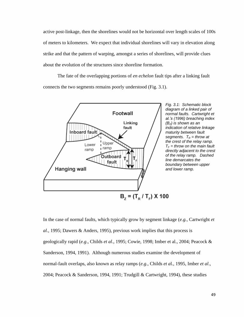
49

active post-linkage, then the shorelines would not be horizontal over length scales of 100s

of meters to kilometers. We expect that individual shorelines will vary in elevation along

strike and that the pattern of warping, amongst a series of shorelines, will provide clues

about the evolution of the structures since shoreline formation.

The fate of the overlapping portions of en echelon fault tips after a linking fault

connects the two segments remains poorly understood (Fig. 3.1).

In the case of normal faults, which typically grow by segment linkage (e.g., Cartwright et

al., 1995; Dawers & Anders, 1995), previous work implies that this process is

geologically rapid (e.g., Childs et al., 1995; Cowie, 1998; Imber et al., 2004; Peacock &

Sanderson, 1994, 1991). Although numerous studies examine the development of

normal-fault overlaps, also known as relay ramps (e.g., Childs et al., 1995, Imber et al.,

2004; Peacock & Sanderson, 1994, 1991; Trudgill & Cartwright, 1994), these studies

Fig. 3.1: Schematic block diagram of a linked pair of normal faults. Cartwright et al.’s (1996) breaching index (BZ) is shown as an indication of relative linkage maturity between fault segments. TR = throw at the crest of the relay ramp. TF = throw on the main fault directly adjacent to the crest of the relay ramp. Dashed line demarcates the boundary between upper and lower ramp.

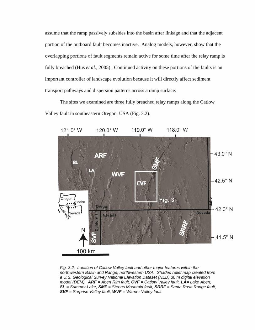
50

assume that the ramp passively subsides into the basin after linkage and that the adjacent

portion of the outboard fault becomes inactive. Analog models, however, show that the

overlapping portions of fault segments remain active for some time after the relay ramp is

fully breached (Hus et al., 2005). Continued activity on these portions of the faults is an

important controller of landscape evolution because it will directly affect sediment

transport pathways and dispersion patterns across a ramp surface.

The sites we examined are three fully breached relay ramps along the Catlow

Valley fault in southeastern Oregon, USA (Fig. 3.2).

Fig. 3.2: Location of Catlow Valley fault and other major features within the northwestern Basin and Range, northwestern USA. Shaded relief map created from a U.S. Geological Survey National Elevation Dataset (NED) 30 m digital elevation model (DEM). ARF = Abert Rim fault, CVF = Catlow Valley fault, LA= Lake Abert, SL = Summer Lake, SMF = Steens Mountain fault, SRRF = Santa Rosa Range fault, SVF = Surprise Valley fault, WVF = Warner Valley fault.

51

The ramps are footwall breached, meaning the linking fault extends from the inboard

fault tip to the outboard fault and breaks the upper portion of the ramp. This orientation

is the expected way a linking fault breaches a ramp based on numerical models (Crider &

Pollard, 1998). The sites we chose cover a range of linkage scenarios from a relatively

immature linkage to relatively mature one. Our purpose is to examine shoreline elevation

changes relative to segment linkage to investigate how the ramp deforms post-linkage

and where that deformation occurs within the relay ramps over geomorphic timescales.

3.2 Geological Setting

The study area is in the Catlow Valley located within the Basin and Range in

southeastern Oregon, USA (Fig. 3.2). The Catlow Valley fault is a ca. 65 km long, north-

south striking normal fault system (Fig. 3.3) that displaces lava flows associated with the

16.6 ± 0.02 Ma old Steens basalt (Hooper et al., 2002). The topographic expression of the

fault system is a steep escarpment, up to several hundred meters high. It is made up of at

least six linked segments; unfortunately there is no direct slip rate information on any of

these segments. Fault chronology is not directly known but we bracket fault initiation to

between 16.6 and approximately 10 Ma, using the age of the Steens basalt (Hooper et al.,

2002) and the onset of Basin and Range extension in southeastern Oregon (Scarberry et

al., 2010). A population of northwest striking faults, smaller in scale than the Catlow

Valley segments, is present but do not appear to have any structural control over the

Catlow segments. We interpret these faults as being related to the Brothers fault zone,

which is zone of distributed normal faults that are generally more pronounced northwest

of Catlow Valley (Scarberry et al., 2010; Weldon et al., 2002).

52

Fig. 3.3: Shaded relief map of Catlow Valley fault (based on the 10 m DEM), showing the maximum extent of Paleolakes Catlow and Alvord based on the highest late Pleistocene shorelines in the basins. The extent of Paleolake Alvord here is similar to previous interpretations of the late Pleistocene extent of that lake (Reheis, 1999; Reheis et al. 2014.

53

3.2.1 Paleolake Catlow and other Pleistocene northwestern Basin and Range pluvial

lakes

Pluvial lake shorelines are present along the Catlow Valley fault escarpment

(Vander Meulen et al., 1988); as many as seven can be observed in some locations but

not all are spatially extensive (Fig. 3.4).

These shorelines are evidence that a substantial lake (10s of km in width and length and

up to 50m deep) once occupied Catlow Valley in the geologically recent past. The

shorelines are prominent features along the Catlow escarpment (Fig. 3.4a), extending for

Fig. 3.4: (a) Google Earth perspective of relay ramp ‘A’ showing seven well preserved shorelines on the outboard fault scarp. Although seven shorelines are noted here they are not all spatially continuous along strike. Arrows point to individual shoreline inner edges. Field of view shown in Fig. 3.6a. (b) Field photograph showing a Catlow Valley shoreline. Note differences in color of terrace tread and terrace riser due the abundance of sand versus basalt boulders. The location of this photograph is south of relay ramp ‘C’, its location is noted in Fig. 3.3.

54

10s of km and are visible in aerial imagery and digital elevation models (DEMs). These

terraces are likely associated with the ultimate regression of Paleolake Catlow. Little

information exists on the paleolake and what work does exist only acknowledges the

presence of shorelines (Vander Meulen et al., 1988). Two key pieces of information

indicate that the shorelines formed during the last lake cycle regression. This is also why

the shorelines are appropriate features to use for this study. One, the shorelines are very

well preserved for long distances along the fault escarpment. If the shorelines have been

altered by hillslope processes, these will act over the entirety of the shorelines, and any

degradation in elevation is expected to be relatively uniform along the escarpment. Thus

elevation differences along a particular shoreline will reveal where more deformation has

accumulated (as reflected by shoreline warping). The second piece of information is the

fact that the shorelines are not superimposed over one another. The key observation here

is that if there were shorelines associated with older lake cycles we would expect to see

older, warped shorelines with younger, less deformed ones superimposed over them.

Because we do not observe this phenomenon, we conclude that the shorelines along the

Catlow Valley fault segments were formed during the ultimate lake cycle regression.

Other large pluvial lakes existed during the late Pleistocene in the northwestern

Basin and Range (Adams & Wesnousky, 1998; Carter et al., 2006; Ibarra et al., 2014;

Licciardi, 2001; Oldow & Singleton, 2008; Reheis et al, 2014). Catlow Valley is in close

proximity to Alvord Basin, located a few 10s of km to the east (Fig. 3.3). These two

fault-controlled basins share a common footwall, the Steens Mountain fault block, which

experienced late Pleistocene glaciations (Evans & Geisler, 2001). U-shaped valleys

created during these glaciations terminate in both basins, thus Paleolake Catlow would

55

have experienced climatological and hydrological conditions similar to that of late

Pleistocene Paleolake Alvord. Two sets of shorelines, known as the Serrano and Alvord

terraces, are recognized along the Steens Mountain fault escarpment in the Alvord basin.

The Alvord terraces are distinct in that the Serrano terraces are topographically higher,

more discontinuous, and channelized by fluvial erosion, whereas the Alvord terraces are

topographically lower, well-preserved, and have not been significantly degraded by

fluvial erosion (Oldow & Singleton, 2008). The Alvord terraces are thought to have

formed between 20 and 11 ka, whereas the Serrano terraces are thought to have formed

about 130-200 ka (Oldow & Singleton, 2008). The Catlow Valley shorelines are

probably of very similar age to the Alvord terraces and nearby Paleoakes Surprise and

Chewaucan (see Interpretations & Discussion).

A requirement for our study is that the shorelines must be younger than the

linking faults that breach the ramps. Although we have no direct age constraints on the

shorelines or faults, we argue that the linking faults must be significantly older than the

shorelines. We reach this conclusion based on two primary pieces of evidence. First,

normal faults arrange themselves into en echelon patterns and begin linking very early in

the evolution the fault system (Cowie, 1998) and Catlow Valley fault has likely evolved

over millions of years (Scarberry et al., 2010). Conversely, shorelines in Alvord Basin,

other nearby lacustrine basins, and Catlow Valley, date to the late Pleistocene (Reheis et

al., 2014). From this it is clear that the fault linkage events considerable predate

shoreline formation.

56

3.3 Data and Methods

High resolution 1 m digital orthophoto quarter quadrangles (DOQQs), a 10 m

digital elevation model (DEM) and field observations are utilized to map deformed

pluvial lacustrine shorelines along the Catlow Valley fault escarpment. The DOQQs and

DEM are products of the U.S. Geological Survey National Elevation Dataset (NED). The

geomorphic feature that we mapped is the slope break between the various terrace risers

and terrace treads, here termed inner edges (Fig. 3.5a). We chose this because the inner

edges give the best representation of paleohorizontal because there is a definable

relationship between the inner edges and the lake surface when the individual shorelines

formed (e.g., Adams & Wesnousky, 1998, Hare et al., 2001). The shorelines that are

mapped in this study are ones that are most continuous along fault strike and that can be

mapped on either side of the site of fault linkage along the breached relay ramps. It is

important to note that we are interested only in deviations of individual shorelines from

horizontal rather than changes in elevation between shorelines; interpretations based on

the latter would require assumptions about lake volume and a complete chronology.

Our field sites consist of three relay ramps that have been completely breached by

linking faults. The sites span a range of linkage scenarios from a relatively immature

linkage to mature ones. We characterize linkage maturity by utilizing Cartwright et al.’s

(1996) breaching index (BZ), which is the ratio of throw measured at the crest of a

breached relay ramp (TR) to throw on the adjacent fault (TF), multiplied by 100 (Fig. 3.1).

The purpose of BZ is to convey the relative stages of fault linkage evolution in a

segmented fault system. In other words, for breached relay ramps within the same fault

system, we can assign values of BZ and use it to discern the relative maturity of linkages

57

(Cartwright et al., 1996). This provides the ability to compare deformation patterns

across an evolutionary spectrum of breached relay ramps. To assess where the

deformation is accumulating geometrically, each relay ramp is divided into two regions,

upper and lower, based on the fault geometry. The division (Fig. 3.1) demarcates the

regions of the relay ramps that are bounded by the inboard and outboard segments

(lower) and the outboard and linking segments (upper).

We utilize ArcGIS v. 10.0 to display and analyze the DOQQs (Fig. 3.5b), the

DEM and the derivative maps (slope and curvature maps) generated from the DEM.

58

The shoreline inner edges are located and mapped using a combination of the DOQQs

and a curvature map. We use these two data types in conjunction with one another

because they offer the most straightforward and objective way of both identifying and

mapping the inner edges. The DOQQs are useful because terrace rises are darker in color

due to the abundance of basalt boulders, whereas treads are lighter in color due to the

presence of sandy material. We clearly see this distinction in our field observations (Fig.

3.4b). The curvature map is useful because we can classify the morphology of the

shorelines objectively based on the DEM. We classify the curvature map such that we

can display zero and negative curvature separately from positive curvature. Positive

curvature indicates a surface is concave up whereas negative curvature indicates a surface

is concave down. A curvature of zero indicates a flat surface (Fig. 3.5c). By displaying

the curvature in this manner we map the interface between positive and negative/zero

curvature, which is the shoreline inner edge. We then drape the curvature map over the

DOQQ to map shoreline inner edges. In areas where the curvature map and DOQQs

deviate on the position of the inner edge, we map it using the DOQQ because the

resolution is higher (1 m/pixel).

Shoreline inner edge elevation data are extracted from the DEM and plotted.

With regards to the elevation data, we make two considerations. First, we consider

Fig. 3.5: (a) Schematic block diagram of a flight of shorelines and their features. (b) 1 m/pixel Digital Orthophoto Quarter Quadrangle (DOQQ) of mapped shoreline inner edges (black lines). (c) Schematic cartoon of a shoreline in profile view. The shoreline features are indicated as well as areas of zero, negative and positive curvature. The interface between positive curvature and zero-negative curvature demarcates the shoreline inner edge and facilitates mapping. (d) Curvature map draped over the same DOQQ shown in part ‘b’. Note the interface between curvature classes coincides with our field observation of terrace treads and risers (sand vs. boulders) as noted in undraped DOQQ. In rare instances where curvature map and DOQQ disagree we mapped the features using the DOQQ because the resolution is higher. DOQQ courtesy of U.S. Geological Survey.

59

vertical deformation of these shorelines to be only minimum measurements, because

hillslope diffusion and mass wasting along the Catlow Valley fault escarpment has

presumably altered inner edge elevation. There is field evidence of talus above some

shorelines. In particular, we avoided mapping the uppermost shoreline, which is the most

heavily affected and obscured by this material. Although we have no way of knowing

how much they have been altered, we are confident that these processes should have

affected our study sites similarly. This is because the factors that would drive different

rates of erosional processes (i.e., slope morphology and climate) are presumed to not

change from site to site in our study area. With this in mind, although we may only

capture minimum values of vertical deformation, we still gain invaluable insight into

relative amounts of deformation between the field sites.

A second consideration is error. We use a 2 m error to account for the vertical

resolution of the DEM and vertical error related to the inner edge relationship to water

surface. Land cover in the study area is mostly grassland with some shrubs, and the

standard deviation of vertical accuracy for NED data for these two land cover classes is

1.55 m and 2.17 m, respectively (Gesch et al., 2014). Due to the fact the study area is

mostly grassland, we are confident that a 2 m error accounts for the vertical error in the

DEM. Another source of error that must be addressed is variability in the elevation of the

inner edge relative to the paleolake level. Previous work has shown that there is a

consistent difference between the elevation of inner edges and mean water level. For

example, Locke & Meyer (1994) show that for 105 modern inner edge elevation

measurements, the inner edges are, on average, 1.8 ± 0.3 m above mean lake level.

Similarly, Hare et al. (2001) found that inner edge elevation was on average 1.3 ± 0.4 m

60

higher than what those authors interpreted as paleolake level. A 2 m margin of error,

therefore, captures well shoreline elevation variability due to DEM vertical resolution and

geomorphic relationships. Other authors have also noted similar errors (~2 m) between

water level and constructional shoreline sedimentological features in both modern and

ancient shorelines (Adams & Wesnousky, 1998; Atwood, 1994). This lends support to

our use of a 2 m error and we are confident that potential geomorphic variability is

captured by this error.

Although we show several shorelines at similar elevations from different sites, we

make no attempt to correlate them to one another. Additionally, we do not map all of the

shorelines at all the sites. For this work we simply use the warping patterns (outside of a

2 m error) of individual shorelines as proxies of fault slip. Shorelines were excluded

because they cannot be mapped on both sides of the site of fault linkage or the shoreline

is discontinuous and cannot be objectively identified in remote sensing data.

The location of the fault trace with respect to the shorelines is not precisely

known at our sites. The shorelines likely meander between the footwall and hanging wall

of the fault, which makes mapping of the fault trace difficult. We can infer in some

locations that the fault trace lies between two adjacent shorelines if a topographically

higher shoreline is up warped and an adjacent, lower shoreline is down warped. Each

data plot is marked with lines with arrowheads showing where streams have incised into

the shorelines; these localized areas are not taken into consideration when describing the

shoreline deformation patterns.

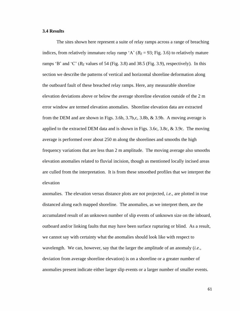
61

3.4 Results

The sites shown here represent a suite of relay ramps across a range of breaching

indices, from relatively immature relay ramp ‘A’ (BZ = 93; Fig. 3.6) to relatively mature

ramps ‘B’ and ‘C’ (BZ values of 54 (Fig. 3.8) and 38.5 (Fig. 3.9), respectively). In this

section we describe the patterns of vertical and horizontal shoreline deformation along

the outboard fault of these breached relay ramps. Here, any measurable shoreline

elevation deviations above or below the average shoreline elevation outside of the 2 m

error window are termed elevation anomalies. Shoreline elevation data are extracted

from the DEM and are shown in Figs. 3.6b, 3.7b,c, 3.8b, & 3.9b. A moving average is

applied to the extracted DEM data and is shown in Figs. 3.6c, 3.8c, & 3.9c. The moving

average is performed over about 250 m along the shorelines and smooths the high

frequency variations that are less than 2 m amplitude. The moving average also smooths

elevation anomalies related to fluvial incision, though as mentioned locally incised areas

are culled from the interpretation. It is from these smoothed profiles that we interpret the

elevation

anomalies. The elevation versus distance plots are not projected, i.e., are plotted in true

distanced along each mapped shoreline. The anomalies, as we interpret them, are the

accumulated result of an unknown number of slip events of unknown size on the inboard,

outboard and/or linking faults that may have been surface rupturing or blind. As a result,

we cannot say with certainty what the anomalies should look like with respect to

wavelength. We can, however, say that the larger the amplitude of an anomaly (i.e.,

deviation from average shoreline elevation) is on a shoreline or a greater number of

anomalies present indicate either larger slip events or a larger number of smaller events.

62

3.4.1 Relay Ramp ‘A’

Figure 4.6 shows the elevation profiles of the inner edges of four shorelines along

the most immature breached relay ramp (BZ = 93). The four shorelines are designated

A1, A2, A3, and A4. A1 is the lowest topographically and A4 is the highest. Variation

in shoreline inner edge elevation is most variable on the upper shorelines (A3 and A4;

Fig. 3.6). Shorelines A4 and A3 contain 4 elevation anomalies each that deviate as much

as 2 m from average shoreline elevation outside of the 2 m error window (Fig. 3.6c).

Shoreline A2 contains only 2 anomalies (< 2 m, but outside of the 2 m error) and

shoreline A1 contains no anomalies.

We do not see a ubiquitous pattern where up-warping on a shoreline is met with

spatially consistent down-warping on a topographically lower shoreline. We expected

that the fault trace would up-warp a shoreline on the footwall and down-warp a shoreline

on the hanging wall. However, it is difficult to find a surface expression of the fault trace

this way. The absence of this pattern indicates a complex trace expression (i.e., multiple

bifurcating and/or discontinuous splays) of the fault in the near-surface or, on the other

hand, that the fault is blind. Although there are areas locally within relay ramp ‘A’ where

up-versus down-warping patterns are associable between shorelines, this pattern is

sustained, vertically only through, at most, two shorelines. Most of the anomalies are

clustered within 2 km on either side of the site of fault linkage. There are noticeably

more anomalies (5 total) in shoreline elevation between the site of fault linkage and the

boundary between the upper and lower ramp. There are only 2 anomalies in the lower

ramp.

63

64

Figure 3.7a shows two shorelines, R1 and R2, located within relay ramp ‘A’ that

are therefore useful in addressing the tilting of the relay ramp. For the most part, the

shoreline inner edges do not vary in elevation outside of the 2 m error. The only area

where shoreline elevation change is significant outside of the error occurs between 0 and

100 m on the distance axis of Fig. 3.7b & c. The largest variation in inner edge elevation

is 4 ± 2 m. Based on the direction and amount of inner edge elevation change, the lower

shoreline, R1, is tilted an average of 1.8° toward 290° and the upper shoreline, R2, is

tilted an average of 6.4° towards 329°.

3.4.2 Relay Ramp ‘B’

Figure 3.8 shows the study site map and elevation plots of three shoreline inner

edges located along breached relay ramp ‘B’. Fault segments here are at a more advanced

stage of linkage, which is evidenced by the lower breaching index (BZ = 54). The three

shoreline inner edges mapped at ramp ‘B’ are labeled B1, B2 and B3; B1 is the lowest

topographically and B3 is the highest.

Fig. 3.6: (a) 1 m/pixel DOQQ of relay ramp ‘A’ showing the inboard, linking and outboard faults, and the shorelines that were mapped at this site. The black lines labeled A1-A4 are the mapped shoreline inner edges. (b) Elevation versus distance plots of the shoreline inner edges mapped at relay ramp ‘A’; the error is ± 2 m. Arrows indicate locations of fluvial incision into the shorelines. Values to the right of the plot are the maximum displacements (i.e., the highest elevation anywhere on the shoreline minus the lowest elevation anywhere on the shoreline). Note the dividing line between upper and lower ramp (black dashed line), the site of fault linkage (solid black line), and the contrast in shoreline deformation pattern. (c) Moving average profile of shoreline elevation. Blue box shows ± 2 m error, dashed line is the average elevation of the entire shoreline, ‘X’s show elevation anomalies (i.e., where the moving average deviates from average shoreline elevation by more than 2 m. DOQQ courtesy of U.S. Geological Survey. Also note the zone of more frequent shoreline elevation anomalies is located within 2 km on either side of the site of fault linkage.

65

Shorelines B1 and B3 each contain 2 anomalies, and shoreline B2 contains 1 anomaly

(Fig. 3.8c). There are not as many anomalies in shoreline elevation at ramp ‘B’ as there

are at ramp ‘A’. Three anomalies in shoreline elevation that occur along ramp ‘B’ appear

to be spatially coincident with one another (Fig. 3.8c), but there is no consistent up-

warping or down-

warping pattern. At least half of elevation anomalies are located within 2 km of the site

of fault linkage. None of the anomalies deviate more than 5 ± 2 m from average

shoreline elevation.

Fig. 3.7: (a) Map view of two shorelines (R1 & R2), which are present on relay ramp ‘A’. The location of the shorelines within the relay ramp is shown in Fig. 6. Numbers in white are distances in meters from zero on the x-axis in parts ‘b’ & ‘c’. (b and c) Elevation versus distance plots of shorelines R1 & R2. Shorelines are measurably tilted towards the north-northwest. Arrows in part ‘a’ show direction of greatest tilt and the amount of tilt is noted in degrees. Dashed line shows the average shoreline elevation. DOQQ courtesy of U.S.Geological Survey.

66

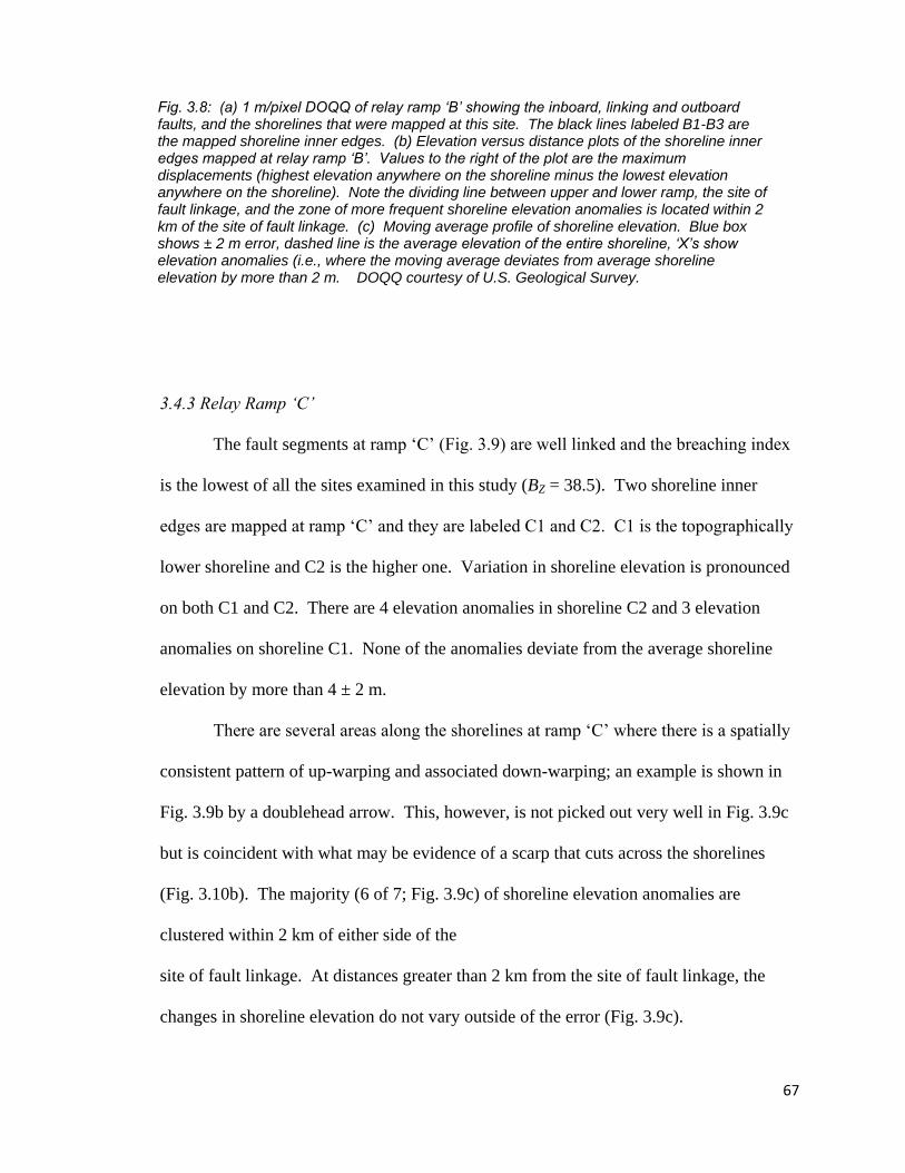
67

3.4.3 Relay Ramp ‘C’

The fault segments at ramp ‘C’ (Fig. 3.9) are well linked and the breaching index

is the lowest of all the sites examined in this study (BZ = 38.5). Two shoreline inner

edges are mapped at ramp ‘C’ and they are labeled C1 and C2. C1 is the topographically

lower shoreline and C2 is the higher one. Variation in shoreline elevation is pronounced

on both C1 and C2. There are 4 elevation anomalies in shoreline C2 and 3 elevation

anomalies on shoreline C1. None of the anomalies deviate from the average shoreline

elevation by more than 4 ± 2 m.

There are several areas along the shorelines at ramp ‘C’ where there is a spatially

consistent pattern of up-warping and associated down-warping; an example is shown in

Fig. 3.9b by a doublehead arrow. This, however, is not picked out very well in Fig. 3.9c

but is coincident with what may be evidence of a scarp that cuts across the shorelines

(Fig. 3.10b). The majority (6 of 7; Fig. 3.9c) of shoreline elevation anomalies are

clustered within 2 km of either side of the

site of fault linkage. At distances greater than 2 km from the site of fault linkage, the

changes in shoreline elevation do not vary outside of the error (Fig. 3.9c).

Fig. 3.8: (a) 1 m/pixel DOQQ of relay ramp ‘B’ showing the inboard, linking and outboard faults, and the shorelines that were mapped at this site. The black lines labeled B1-B3 are the mapped shoreline inner edges. (b) Elevation versus distance plots of the shoreline inner edges mapped at relay ramp ‘B’. Values to the right of the plot are the maximum displacements (highest elevation anywhere on the shoreline minus the lowest elevation anywhere on the shoreline). Note the dividing line between upper and lower ramp, the site of fault linkage, and the zone of more frequent shoreline elevation anomalies is located within 2 km of the site of fault linkage. (c) Moving average profile of shoreline elevation. Blue box shows ± 2 m error, dashed line is the average elevation of the entire shoreline, ‘X’s show elevation anomalies (i.e., where the moving average deviates from average shoreline elevation by more than 2 m. DOQQ courtesy of U.S. Geological Survey.

68

69

3.5 Interpretations & Discussion

Our results show that there is considerable variability in the elevation of

individual shoreline inner edges along the Catlow Valley fault. We attribute elevation

variability, outside of a 2 m error window, to slip on segments of the Catlow Valley fault

system since the shorelines formed. We do see features that we interpret to be surface

scarps (Fig. 3.10), this evidence is limited because the scarps are in close proximity to the

shorelines and have probably been degraded by hillslope processes. In addition, we

cannot discount the possibility of blind slip on portions or perhaps all of the fault

segments.

Although we interpret the majority of the deformation of individual shorelines to

be structurally controlled, we do not want to ignore other processes that may result in

variable shoreline elevation. In the following sections we discuss several issues that may

complicate our interpretations of the spatial distribution of deformation in relation to

relay ramp breaching. The focus is specifically on the shorelines and how they have been

geomorphologically modified since their formation. We will also focus on the surface

expression of the fault and how we reach the conclusion that fault slip is probably a

primary driver of shoreline elevation variability along fault strike. In order to do that,

Fig. 3.9: (a) 1 m/pixel DOQQ of relay ramp ‘C’ showing the inboard, linking and outboard faults, and the shorelines that were mapped at this site. The black lines labeled C1 & C2 are the mapped shoreline inner edges. (b) Elevation versus distance plots of the shoreline inner edges mapped at relay ramp ‘C’. Values to the right of the plot are the maximum displacement of the shorelines. Note the delineation of the upper and lower ramp (dashed black line) and the site of fault linkage (solid black line). Also note the zone of more frequent shoreline elevation anomalies is located within 2 km on either side of the site of fault linkage. (c) Moving average profile of shoreline elevation. Blue box shows ± 2 m error, dashed line is the average elevation of the entire shoreline, ‘X’s show elevation anomalies (i.e., where the moving average deviates from average shoreline elevation by more than 2 m. DOQQ courtesy of U.S. Geological Survey.

70

however, we first establish a time frame over which the deformation occurred, and within

that context discuss the implications for fault and ramp evolution.

3.5.1 Catlow Valley shoreline age and morphology

Fig. 3.10: (a & b) Google Earth views of features that cross-cut shorelines, which we have interpreted as potential scarps. (c) Small faults that breach the surface in the upper portion of relay ramp ‘A’ and small faults that splay off of the main outboard fault. Tick marks on downthrown side.

71

Although we have no direct age constraint on the shorelines in Catlow Valley, we

noted earlier that they are likely of similar age to the Alvord terraces, which have been

dated to between 11 and 20 ka (Oldow & Singleton, 2008), and not the much older 130-

200 ka Serrano terraces. Additionally, the number of shorelines present in Alvord Basin

(5) closely resembles the number of shorelines in Catlow Valley noted by previous

workers (Vander Meulen et al., 1988) and by the present study. This fact suggests that

the ultimate regression in both Paleolake Catlow and Paleolake Alvord was similar

enough to have produced nearly identical numbers of shorelines in both basins. Based on

this, we infer that the shorelines in Catlow Valley are of comparable age to those in

Alvord Basin. In addition, other nearby paleolakes share similar chronologies to Lake

Alvord, which further reinforces our inference. Paleolakes Chewaucan and Surprise were

located about 100 km west-northwest and southwest, respectively, of Catlow Valley.

Dated shorelines associated with the last lake cycle in Surprise Lake suggest the last

highstand was reached about 15 ka (Ibarra et al., 2014). Based on archeological

evidence, Surprise Lake was probably gone by about 6 ka (O’Connell & Inoway, 1994).

Shorelines ages associated with the ultimate late Pleistocene lake cycle of Lake

Chewaucan show that the lake reached highstand probably around 15 ka and entered an

overall decline thereafter (Licciardi, 2001; Negrini, 2002). Although each of these basins

experiences its own distinct hydrological response, the overall picture is that the basins

reached highstand around 10-20 ka. Following highstand the lakes regressed and likely

were gone by the early-mid Holocene. From this, we infer that the Catlow Valley

shorelines are of comparable age to other nearby lacustrine basins (i.e., they probably

formed sometime between 10 and 20 ka). Furthermore, based on this evidence we make

72

the assumption that the higher shorelines are probably older and the lower shorelines are

likely associated with the later stages of the overall late Pleistocene regression. Although

it is possible that the lake transgressed during the overall regression, this would not

greatly impact our interpretations because we are not looking at elevation between

shorelines. Instead, we are concerned with relative amounts of deformation along the

individual shorelines, as reflected by shoreline elevation anomalies along fault strike.

Where a group of shorelines show clustered anomalies suggests it is a site of localized

deformation over 103 - 10

4 years timescale.

Here we also consider whether the anomalies are an artifact of the methodology

or the result of modification by hillslope processes. First, it is difficult to attribute the

anomalies to the measurement methodology. If the observed elevation differences were a

result of the methodology the anomalies would not cluster in certain areas along the fault.

Geomorphic modification of the shoreline elevations is likely, especially with respect to

the inner edges experiencing hillslope diffusion, but we do not think it is the primary

controller of the patterns we observe. We reach this conclusion for two reasons: firstly,

the warping patterns are not randomly distributed along strike and, secondly, they are

associated with a particular structural geometry.

Another potential issue that we must address is whether the variability in

shoreline elevation is associated with lake processes. The first order control on shoreline

formation and elevation is of course associated with the volume of the lake when each

individual shoreline formed. These standstills in lake volume formed the wave cut

terraces that define the inner edges and risers. It has been shown that shoreline elevations

can be affected by lake feature parameters such as fetch, shoreline orientation, local

73

slope, and sediment supply (Reheis et al., 2014 and references therein). In the case of the

Catlow Valley study sites, all three sites are approximately west facing, the only

outcropping rock is basalt, and the fault escarpment is a few 100s m high at all three

locations. The only thing that is significantly different between sites is fetch (distance

that wind is blowing over water). Based on Fig. 3.3, fetch would have been largest over

sites ‘A’ and ‘B’, but these sites show no overwhelming difference in the height of

elevation anomalies than site ‘C’. Furthermore, if lake processes were responsible for the

elevation anomalies, the anomalies would be random, but they are not, they are clustered

with respect to the fault geometry. It is for this reason that we do not interpret the

elevation differences of the Catlow Valley shorelines to be explained primarily by this or

any other geomorphic mechanism.

3.5.2 Shoreline deformation patterns as surface expressions of the Catlow Valley fault

Although we are confident in our age inferences on the Catlow Valley shorelines,

we cannot constrain the geometry of the fault trace with respect to the shorelines. In

some cases there is evidence of where the fault trace is located based on the warping

patterns (Fig. 9), but the patterns are not laterally continuous. Therefore, any mapped

interpretation of the fault trace would be speculative. We do not make an attempt to map

the fault trace with respect to the shorelines because multiple shorelines are likely on both

the hanging wall and footwall of the fault. Additionally, because the trace is likely in

colluvium its geometry is likely complex, consisting of multiple splays that may have

slipped at different times. These complexities preclude any mapping of the trace

geometry using the shoreline deformation patterns. Nonetheless, the pattern of shoreline

74

deformation is valuable. While we cannot directly link the deformation to any single slip

event, anomalies in shoreline elevation from the average shoreline elevation are strong

indicators of slip.

Figures 4.10a & b show two locations where we have interpreted what may be

surface expressions of the fault trace. Although subdued, these features are not like

shorelines in that they are relatively short (100s of m) and appear to cross-cut one or

more shorelines. Because we do not observe cross-cutting shorelines along this

escarpment, we posit that these features may be fault scarps. This evidence, though

limited, and if correct, suggests the fault does have an expression of surface rupture since

ca. 10-20 ka. However, most evidence of surface rupture (i.e., fresh, intact scarps) has

likely been degraded or is simply difficult to observe in remote sensing data due to the

close proximity of the shorelines. One alternate possibility is that fault trace may simply

be higher on the escarpment (i.e., above the shorelines) and may not be discernable. We

cannot rule out the possibility that slip on the Catlow Valley segments has been

predominantly blind and no or relatively few surface-rupturing earthquakes have

occurred since the late Pleistocene. Blind slip could still be manifest by the warping of

the shorelines.

3.5.3 Along strike pattern of deformation: Implications for fault evolution over

geomorphic timescales

Here we discuss the along strike pattern of fault related deformation of the

Paleolake Catlow shorelines and discuss the implications for fault growth and evolution

over the geomorphic timescale. One of the most obvious features of the shoreline

75

elevation plots is that the largest number of anomalies occurs within about 2 km on either

side of the site of fault linkage at all 3 study sites. In relay ramp ‘A’ the shorelines show

significant elevation variability between 2 km and 4 km from the outboard fault tip (Fig.

3.6b & c). There are also fewer elevation anomalies in shoreline elevation from 0 to ~ 2

km along the distance axis of Fig. 3.9c. The majority of anomalies at ramp ‘B’ do not

appear clustered along strike like in ramps ‘A’ and ‘C’. One reason this may be is that

the faults that bound ramp ‘B’ are at a fairly high obliquity to one another. The obliquity

of the faults suggests that the inboard fault may have propagated toward the outboard

fault resulting in their linking. This would negate the need for initiation of an oblique

linking fault and small upper ramp faults would be unnecessary to localize a linking fault.

We argue that the reason there appears to be a 2 km length control on the

locations of anomalies is due to the fault geometry and the presence of smaller faults

within the ramp (Fig. 3.10c). Although the small faults are only observable on ramp ‘A’,

we are likely not observing faults that may have accrued blind slip. We expect that small

blind faults might also be present on ramp ‘B’ and ‘C’. The obliquity at of the faults at

ramp ‘B’, however, may preclude the development of small relay faults, which would

explain the lack of clustering of shoreline elevation anomalies. We posit that the upper

ramp is subjected to deformation mainly associated with the linking and outboard faults,

as well as any smaller faults present within the upper ramp. We can explain the observed

differences in shoreline deformation between the upper and lower ramp if we imagine

how slip is partitioned between the different structures (Fig. 3.11b & c).

If the outboard fault becomes inactive post linkage, the shorelines are expected to

passively

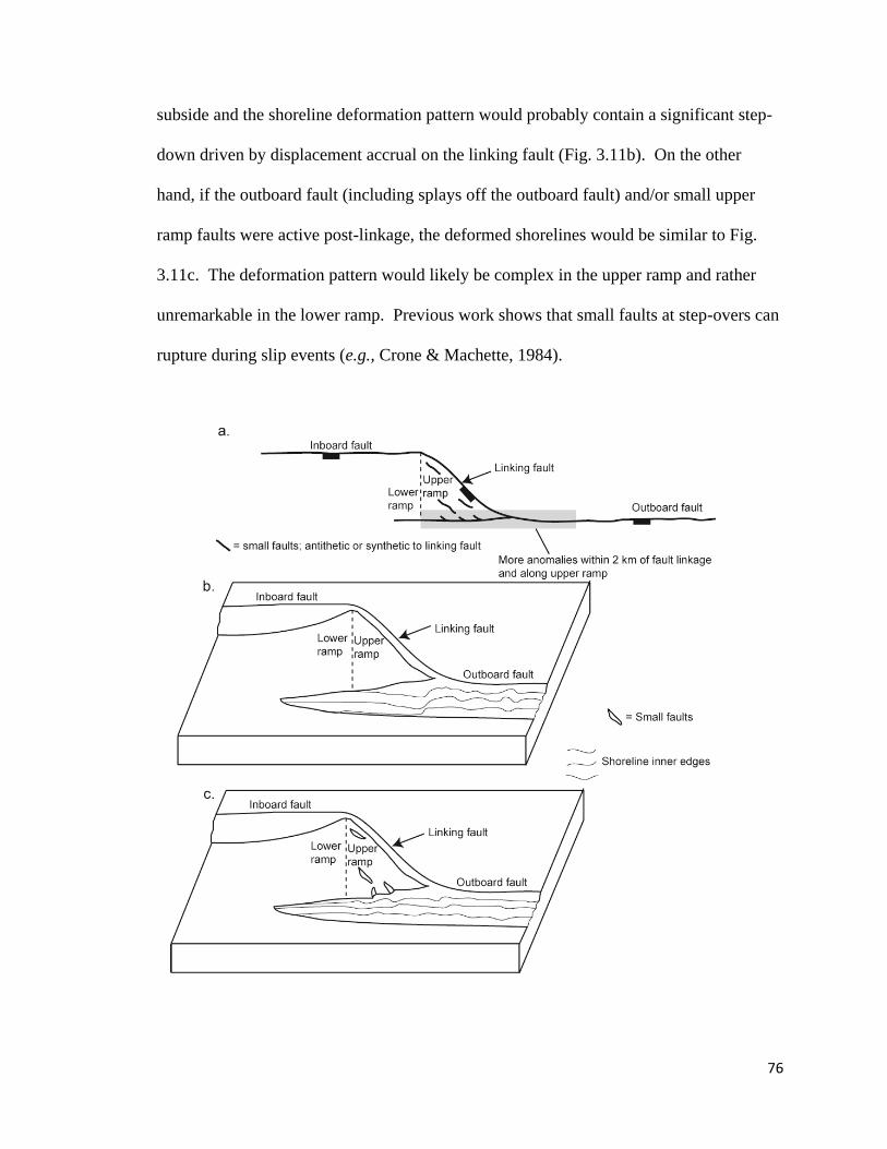
76

subside and the shoreline deformation pattern would probably contain a significant step-

down driven by displacement accrual on the linking fault (Fig. 3.11b). On the other

hand, if the outboard fault (including splays off the outboard fault) and/or small upper

ramp faults were active post-linkage, the deformed shorelines would be similar to Fig.

3.11c. The deformation pattern would likely be complex in the upper ramp and rather

unremarkable in the lower ramp. Previous work shows that small faults at step-overs can

rupture during slip events (e.g., Crone & Machette, 1984).

77

Therefore, slip on these faults, either synthetic or antithetic to the linking fault (Figs.

4.10c & 4.11) would lead to a complex pattern of shoreline warping within the upper

ramp. Because we do not observe the shorelines passively subsiding into the basin (as

illustrated in Fig. 3.11b) the most likely conclusion is that the outboard fault and/or small

ramp faults do remain active post-linkage. The linking, outboard, and smaller ramp faults

may not all slip during the same event(s). Our primary observation is that over

timescales of 103 - 10

4 years, deformation has not yet definitively localized on the linking

faults, despite the presence of well-established structures.

Our results also show that a relay ramp surface is highly dynamic and the way in

which the ramp surface deforms is complex. The deformed shorelines R1 and R2 at ramp

‘A’ indicate that the lower ramp appears to progressively tilt toward the hanging wall by

a few degrees. This degree of tilt is not unrealistic (Fossen & Rotevatn, 2016). Our

measurements of ramp tilt are located on the lower ramp and are not spatially extensive,

so we cannot say that the whole ramp surface is deforming in this manner. However, our

Fig. 3.11: (a) Schematic map view of a pair of normal faults (inboard and outboard) that are connected by a linking fault (rectangles on downthrown side) and the associated relay ramp. Small black lines are faults on the upper ramp that may be synthetic or antithetic to the linking fault. The majority of shoreline elevation anomalies are observed occur within about 2 km on either side of the site of fault linkage. (b) Block diagram of how shoreline deformation would be expected to look in the absence of activity on the outboard fault or any faults within the upper relay ramp (only the linking fault is active). Shorelines would passively subside and would be expected to contain a large step-down at the transition from the outboard-linking intersection to the inactive outboard tip (c) Block diagram of how shoreline deformation would be expected to look if the outboard fault, linking fault and small ramp faults (or any combination thereof) remained active post-linkage. Regardless of the combination, the deformation pattern suggests that slip has yet to localize on linking faults at all three study sites despite the presence of fully formed linking structures. If we consider a hypothetical earthquake, which nucleates on the outboard fault and propagates toward the relay, it may rupture the outboard segment, the linking segment, smaller faults on the ramp, or all of them. We interpret the differences in shoreline deformation patterns between the upper ramp and lower ramp, post-linkage, to be a result of earthquakes that may rupture some or all of those structures. The implication here is that following linkage, the outboard fault tip and structures within the former relay ramp itself remain active over geomorphic timescales.

78

data on the upper ramp (shoreline elevation anomalies) show that, at least over

geomorphic timescales, the ramp is not deforming coherently post-linkage.

Ultimately, we show that the geometry of the linking structure with respect to the

overlapping faults has an impact on how the ramp deforms. These observations

specifically apply to those relays that are footwall breached, which are expected to be

common based on numerical models of Crider and Pollard (1998). Furthermore, our data

add to the understanding of the progression of relay ramp deformation. Whereas we

know that the way in which a relay ramp initially deforms is dictated by how slip is

partitioned between uplift and subsidence on both faults (Ferrill & Morris, 2001), relay

ramps post-linkage had been thought to deform as passive structures, which rotate and

subside in response to slip on the now linked segments (Imber et al., 2004). Our data,

however, show that the ramps are not deforming as passive structures. Rather than

simply subsiding into the basin, the outboard fault tip and/or small faults within the upper

ramp continue to be active after fault linkage. In either case, this implies that over the

geomorphic timescale that we have examined, slip has yet to fully localize on the linking

structures, despite the presence of fully formed linking faults. Our observations indicate

that post-linkage relay ramp evolution is more complex than previously assumed.

3.6 Conclusions

In conclusion, we attribute deformation of lacustrine shorelines to slip along

segments of the Catlow Valley fault. We find that fault linkage maturity does not have a

significant effect on the vertical or horizontal distribution of deformation along breached

relay ramps. We do not observe a distinct difference in the overall pattern of deformation

79

that can be explained by a difference in maturity of the linking faults. Areas of numerous

shoreline elevation anomalies are indications that the linking, outboard, or small relay

ramp faults are likely active over the same time frame. Furthermore, our work shows that

the portion of the outboard fault that would be expected to be inactive after linkage

actually remains active for up to 104 years. This is evidenced by the presence of

anomalies in individual shoreline elevation along the outboard fault tip. Additionally,

this study shows that slip has yet to fully localize on the linking faults despite the

presence of fully formed breaching faults. Finally, these results show that relay ramps

are not passively deforming structures following fault linkage. Our work indicates that

the ramp continues to deform post-linkage, either along the portion of the outboard fault,

which previous studies had presumed to be inactive, or along small ramp faults.

80

Chapter 4

The role of fault scale, overlap and spacing in controlling extensional relay ramp

fluvial system geometry

Abstract

Differences in the geometry of fluvial systems that drain extensional relay ramps are

attributed to the scale of the ramp bounding fault segments, the spacing between

segments and the amount of overlap between segments. Previous conceptual models for

relay ramp geomorphological evolution have assumed that ramp fluvial catchments

develop on the ramp surfaces and flow parallel to fault strike into the adjacent basin.

Numerous examples exist in nature, however, that show that this is not ubiquitous. The

fundamental question of what drives this geomorphic difference has, to date, not been

fully addressed. We selected 27 relay ramps across the Basin and Range and mapped the

faults and ramp fluvial systems associated with each site. The sites represent a range of

fault scales, which we define by the total outboard fault length, and a range of spacing

and overlap values in order to better understand the structural controls on ramp fluvial

system geometry differences. Results show that outboard fault length less than about 15

km is a useful predictor for whether the majority of a relay ramp surface drains parallel to

fault strike or will traverse the outboard fault. High overlap/spacing ratios are associated

with relays along shorter (< 15 km long) outboard faults, whereas lower overlap/spacing

ratios are associated with relays along longer faults. The relationship between

overlap/spacing and fault scale suggest that lower overlap/spacing value relays may be

more common along longer outboard faults because they survive for longer periods of

81

time in the landscape. Our geomorphological observations can be used to predict synrift

depocenter locations along segmented faults, but it only appears to be applicable to short

(<15 km long) fault segments and in early rifting stages. At longer fault lengths, ramp

fluvial system geometry has no discernable relationship with from any specific structural

parameter.

4.1 Introduction

Relay ramps are structural features that occupy the area between overlapping

normal fault segments (Larsen, 1988). These features are commonly exploited by fluvial

systems that take advantage of the low points in topography and drain a part of the

footwall block. The fluvial systems, therefore, utilize the ramps as corridors for sediment

transport into the adjacent hanging wall basin (Gawthorpe & Hurst, 1993; Gupta et al.,

1999; Cowie et al., 2006; Elliot et al., 2012). The prevailing conceptual model for relay

ramp surface evolution holds that fluvial systems develop on the ramp and in the

immediate footwall, and are oriented such that flow is parallel to fault strike (i.e.,

Gawthorpe & Hurst, 1993; Fig 4.1a & b). However, there are examples of relay ramp

fluvial systems that are oriented such that the majority of the ramp area drains across the

outboard fault scarp (Fig. 4.1c). Fault-transverse fluvial systems have been previously

described by Jackson & Leeder (1994), Densmore et al. (2003) and Athmer & Luthi

(2011). The fundamental control on these different fluvial geometries, why they exist,

and what mechanisms are at play, has never been previously explored. This study

examines basic structural geometry (fault scale, fault spacing and overlap) and how they

are related to differences in fluvial system geometry.

82

Understanding the evolution of ramp surfaces and how they develop temporally

and spatially is of particular interest because of their role in governing sediment transport

in evolving continental rift basins. Predicting these synrift sediment transport pathways

and depositional patterns is useful because it is applicable to predicting various parts of

hydrocarbon systems.

In the traditional conceptual model (Gawthorpe & Hurst, 1993), a relay catchment is

geometrically controlled by the ramp adjacent faults and develops a large alluvial fan or

Fig. 4.1: Block diagrams of a relay ramp fluvial systems along an outboard fault that are: (a) shorter than 20 km and (b & c) longer than 20 km. These diagrams illustrate the hypothesized relay catchment geometries as a function of outboard fault length. These diagrams also illustrate how it is thought a fault-parallel dominated catchment may transition to a fault-transverse dominated catchment.

83

fan-delta at the toe of the ramp. Although there are examples of relay ramp-parallel

fluvial systems, it is far from a ubiquitous observation, as noted above.

The majority of previous work on relay ramp structure and evolution has focused

on controlling mechanisms of ramp orientation as a consequence of fault interaction and

linkage (e.g., Trudgill and Cartwright, 1994; Cartwright et al., 1996; Ferrill & Morris,

2001) and ramp bounding fault overlap and spacing geometry (Soliva et al., 2006; Long

& Imber, 2011; Fossen & Rotevatn, 2016). Previous studies have also sought to find the

interconnections between the structural development of rift basins through fault

interaction and linkage and synrift sedimentary architecture (Gupta et al., 1998; Dawers

& Underhill, 2000; McLeod et al., 2002; Cowie et al., 2006). What is lacking, however,

is that there has been no systematic examination of the controls on relay fluvial geometry,

in spite of the implications for rift basin stratigraphic architecture. We hypothesize that

particular structural parameters such as the outboard fault length, fault overlap and fault

spacing are the primary controls on these differences. To test this, we select a suite of

sites throughout the Basin and Range province, western North America, to evaluate

which structural parameter(s) is (are) associated with different ramp fluvial system

geometries.

4.2 Geological Setting

This study examines 27 sites located within the Basin and Range continental rift

system. The sites were chosen for a variety of reasons, the primary ones being good

exposure of the faults, intact fluvial networks on the relays, and scale of the faults.

Figure 4.2 shows the general location of each site and Appendix B (Figs. B1-B6) contains

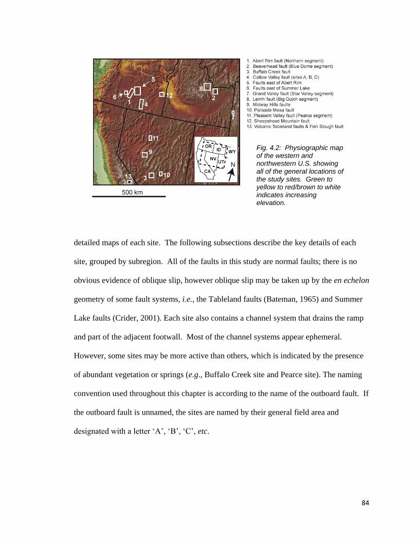
84

Fig. 4.2: Physiographic map of the western and northwestern U.S. showing all of the general locations of the study sites. Green to yellow to red/brown to white indicates increasing elevation.

detailed maps of each site. The following subsections describe the key details of each

site, grouped by subregion. All of the faults in this study are normal faults; there is no

obvious evidence of oblique slip, however oblique slip may be taken up by the en echelon

geometry of some fault systems, i.e., the Tableland faults (Bateman, 1965) and Summer

Lake faults (Crider, 2001). Each site also contains a channel system that drains the ramp

and part of the adjacent footwall. Most of the channel systems appear ephemeral.

However, some sites may be more active than others, which is indicated by the presence

of abundant vegetation or springs (e.g., Buffalo Creek site and Pearce site). The naming

convention used throughout this chapter is according to the name of the outboard fault. If

the outboard fault is unnamed, the sites are named by their general field area and

designated with a letter ‘A’, ‘B’, ‘C’, etc.

85

4.2.1 Western & Southwestern Basin & Range

4.2.1.1 Volcanic Tableland & Midway Hills

Five sites study sites are located on the Volcanic Tableland, which is located in

northern Owens Valley, California. The Tableland is the upper surface of the ~760 ka old

Bishop Tuff (Sarna-Wojcicki et al., 2000), which is a welded rhyolitic ash-flow tuff. The

surface of the Tuff is characterized by a distributed population of north-south striking

normal faults and a now inactive channel network (Gilbert, 1938; Bateman, 1965). The

channels are thought to have been active at various points in the late Pleistocene (ca 70-

300 ka - Gilpin, 2003). The ramp channels clearly formed in response to fault generated

topography (Fig. B1; Bateman 1965; Pinter & Keller, 1994). For more information on

the Volcanic Tableland, see the Geological Setting section of Chapter 2.

The Midway Hills faults (Fig. B2) are also a distributed population of north-south

striking normal faults, located in southwest Nevada just north of Tonopah. The faults

offset basalts that are of early Miocene to early Pliocene age and the faults thought to

have been active in the Quaternary (Sawyer, 1998, and references therein, Ludington et

al., 2005). The Midway Hills faults are generally short (<10 km) and tend to occur as

distributed segments or in groups of two or three, though some arrays contain more

segments. The timing of channel occupation is unknown, however it is probably not too

dissimilar from the Volcanic Tableland located <150 km to the southwest. The channels

are all locally sourced from the fault footwalls and formed in response to fault generated

topography.

4.2.1.2 Palisade Mesa fault, NV; Buffalo Creek fault, NV; Pearce fault, NV

86

The Palisade Mesa fault site is located along a north-south striking, roughly 20

km long, segmented normal fault within the southwestern Basin and Range. The fault

offsets early Oligocene to early Miocene aged rhyolite (Schell, 1981; Dohrenwend et al.,

1996; Ludington et al., 2005) and some scarps show evidence of late Pleistocene activity

(Dohrenwend et al., 1996). The Buffalo Creek fault site is located along a roughly 30 km

long segmented normal fault; Fig. B3 shows a close up aerial image of the site. The fault

offsets Tertiary to Cretaceous volcanics and plutonic rocks of the Desatoya Mountains

block (Willden & Speed, 1974; Dohrenwend et al., 1992; Lidke, 2000). There is an

extensive drainage system that is developed both in the interior of the relay ramp and

along the front of the Buffalo Creek range. The Pearce site is located along a segment of

the Pleasant Valley fault in north-central Nevada (Fig. B3). The Pearce site is located at

a step over between the Pearce and Tobin fault segments. The site is the location of the

1915 Pleasant Valley, Nevada earthquake, which ruptured portions of at least 4 segments

of the Pleasant Valley fault system (Wallace, 1984).

4.2.2 Northeastern Basin & Range

Figure B4 shows close up aerial imagery of the Grand Valley, Lemhi and

Beaverhead faults. The Star Valley site is located along a step-over of the Grand Valley

fault system. The Star Valley fault is about 40 km long. The fault shows evidence of late

Pleistocene to early Holocene activity in alluvial fans (Piety et al., 1992; McCalpin et al.,

2011).

The Big Gulch relay ramp is located along the Big Gulch and Warm Creek

segments of the Lemhi fault in eastern Idaho (Fig. B4). The Big Gulch segment is the

87

outboard fault in this relay ramp; it is the longest fault segment included in this study at

roughly 63 km long. Although previous literature names multiple segments within this

region (Crone & Haller, 1991), geometrically the segments appear to be continuous along

fault strike so they are combined for the purposes of this study. This relay ramp is also

the largest ramp in this study at over 100 km2.

The Blue Dome relay ramp is located at the southern end of the Beaverhead fault,

a segmented fault system also located in eastern Idaho. The two southern most segments

within the Beaverhead fault are the Nicholia and Blue Dome segments (Fig B4). The

Blue Dome segment forms the outboard fault of the ramp and is roughly 35 km long.

Sedimentary rocks of late Paleozoic and early Mesozoic age are exposed along the

majority of the ramp, and Quaternary rhyolite is exposed at the ramp toe (Reed et al.,

2012). The major range front segments (Blue Dome and Nicholia) show evidence of late

Quaternary activity (Skipp, 1985; Crone & Haller, 1991).

4.2.3 Northwestern Basin & Range

4.2.3.1 Summer Lake & Abert Rim

Seven sites are located within a population of northwest striking normal faults

east of Summer Lake and Abert Rim, Oregon. These faults are located at the

northwestern edge of Basin and Range extension (Crider, 2001). The two sites near

Summer Lake are located within basalt, of which the uppermost flows have been dated to

late Miocene time (6.3 ± 0.4 Ma - Diggles et al., 1990; Crider, 2001). The sites east of

Abert Rim are located within Miocene to Pliocene age rhyolites (Walker & MacLeod,

1991).

88

4.2.3.2 Sheepshead Mountain fault & Catlow Valley fault

The Sheepshead Mountain fault is a 17 km long fault (Fig. B5) and forms the

outboard fault segment of the Sheepshead Mountain relay ramp. The Sheepshead

Mountain fault offsets Miocene basalts and rhyolites that outcrop throughout the ramp

(Walker & MacLeod, 1991). Three sites are located along the Catlow Valley fault, a 65

km long segmented fault system in south-central Oregon, which displaces basalt flows

associated with the 16.6 ± 0.02 Ma old Steens basalt (Hooper et al., 2002) (Fig. B6).

Quaternary activity on the Sheepshead Mountain fault is suggested from air photo

reconnaissance but this evidence is limited (Personius et al., 2002). No definitive

evidence of Quaternary activity can be definitely shown on the Catlow Valley segments

because of paleolacustrine shoreline deposits along the escarpment; however it is

suggested on at least one segment and late Pleistocene lacustrine shorelines deviate

significantly from horizontal (Chapter 3; Hopkins & Dawers, 2016).

4.3 Methods

In order to understand how outboard fault length affects ramp fluvial system

geometry, we first define objective criteria to measure specific features. Below, each

metric is defined and how each one was measured is discussed. For this study,

measurements were made using either a handheld GPS device or were made remotely

using a 10 m digital elevation model (DEM) and 1 m digital orthophoto quarter

quadrangles (DOQQs). All feature measurement and data visualization was done in

ArcGIS version 10.0. Five parameters are measured at each site: outboard fault length,

89

the area of the ramp that drains in a direction parallel to fault strike (AFP), the total relay

ramp area (AR), fault spacing and fault overlap (Fig. 4.3). The outboard fault length is

defined as the length of the outboard fault of a relay ramp as measured from one fault tip

to the other. Fault overlap is measured along the center of the relay ramp and spacing is

distance between the faults as measured at the center of the overlap line (Fig. 4.3a & b).

The majority of measurements of outboard fault length, AFP and AR are made via

remote sensing mapping using DOQQs and a 10 m DEM. Measurements made in the

field are denoted in Table 4.1. However, one issue that greatly affects measurements of

OFL and AR is the location of the fault tips. A fault tip is defined as the point along a

fault where displacement becomes zero. However, displacement may not be zero at the

tip of a remotely imaged scarp as seen in both visible imagery or elevation data. These

problems introduce an unknown error in our measurements of fault length and ramp area

because we do not know how much of the visible scarp (in the DOQQ or DEM)

represents true fault length. By default, this also introduces an error in the overlap

measurements. We can constrain some of this uncertainty by including GPS located fault

tips and examining the differences between faults tips mapped in imagery (DOQQ) alone

and those located using GPS. The GPS device is a handheld Trimble GeoXM 2008

Series, which is capable of 1-3 m vertical and horizontal accuracy. Fault tips were

mapped using the handheld GPS by walking along the footwall of the fault until the

displacement between footwall and hanging wall was no longer visible in the field. A

total of 19 fault tips were located using GPS. In the majority of cases (14 of 19), the fault

length is under measured, in other words the visible scarp in the DOQQ is shorter than

the true fault length.

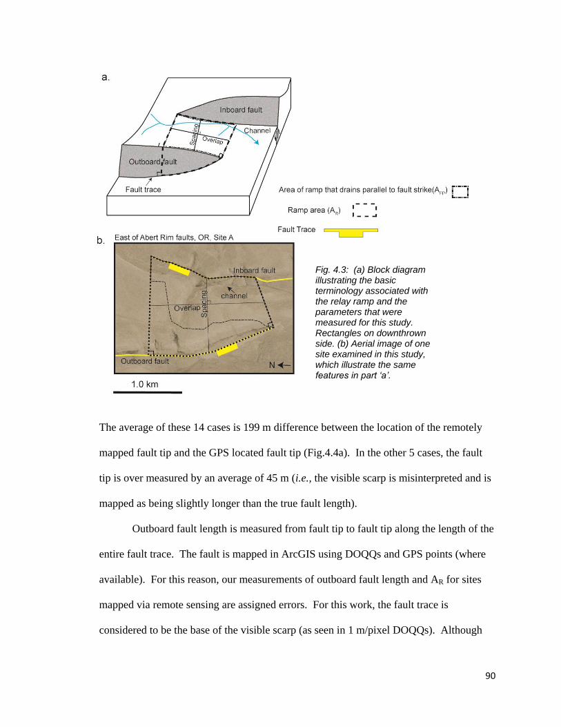
90

The average of these 14 cases is 199 m difference between the location of the remotely

mapped fault tip and the GPS located fault tip (Fig.4.4a). In the other 5 cases, the fault

tip is over measured by an average of 45 m (i.e., the visible scarp is misinterpreted and is

mapped as being slightly longer than the true fault length).

Outboard fault length is measured from fault tip to fault tip along the length of the

entire fault trace. The fault is mapped in ArcGIS using DOQQs and GPS points (where

available). For this reason, our measurements of outboard fault length and AR for sites

mapped via remote sensing are assigned errors. For this work, the fault trace is

considered to be the base of the visible scarp (as seen in 1 m/pixel DOQQs). Although

Fig. 4.3: (a) Block diagram illustrating the basic terminology associated with the relay ramp and the parameters that were measured for this study. Rectangles on downthrown side. (b) Aerial image of one site examined in this study, which illustrate the same features in part ‘a’.

91

this may not be representative of the true fault trace in all cases, it is a consistent means

of mapping the fault along its entire length. Note that the uncertainty in outboard fault

length is only applied where the fault tip is located using DOQQs. In the cases where the

fault tip(s) was located with GPS, no error in length is applied because it is negligible at

the scale shown in the data plots. The maximum uncertainty in fault length for any fault

is, therefore, + 0.398 km (199 m times 2) and – 0.09 km (45 m times 2).

AR is the total area of a relay ramp. AR is measured as the area of a polygon made

up of two lines extending perpendicular from the outboard fault to the inboard fault,

which are then connected to two lines drawn along the fault traces of the inboard and

outboard faults (Fig. 4.3a). The polygon is drawn using DOQQs and the area is measured

in ArcGIS. An example of a ramp area polygon (dashed line) is shown in Figure 4.3b.

Appendix B contains all the mapped relay ramp area polygons used in this study.

Once AR is measured, an uncertainty in the area is applied based on the uncertainty in the

fault tip location. Figure 4.4b shows a schematic illustration of how the uncertainty in

ramp area is derived. Based on the possible over and under estimates of fault tip

locations, we apply a positive and negative ramp area error to the measured areas (Table

4.1). The values of the positive and negative ramp area uncertainties are related to the

average values of under and over measurement of fault tip locations (Fig. 4.4b).

AFP is the area of a polygon that represents the area of the ramp that drains

parallel to fault strike and discharges at the ramp toe (Fig. 4.3a). AFP polygons are

manually mapped in ArcGIS with the aid of a 10 m contour map generated from the

DEM, the DOQQ imagery and ArcGIS’s hydrology tools.

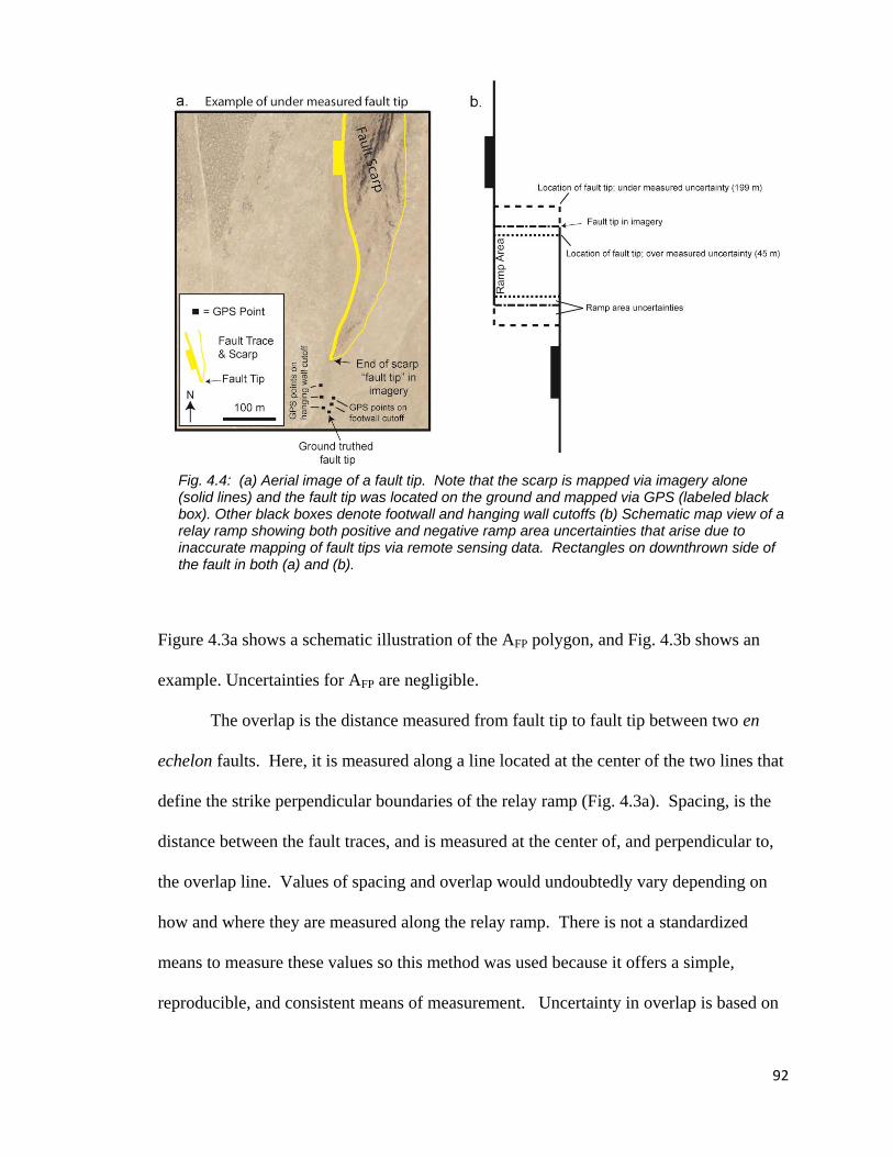
92

Figure 4.3a shows a schematic illustration of the AFP polygon, and Fig. 4.3b shows an

example. Uncertainties for AFP are negligible.

The overlap is the distance measured from fault tip to fault tip between two en

echelon faults. Here, it is measured along a line located at the center of the two lines that

define the strike perpendicular boundaries of the relay ramp (Fig. 4.3a). Spacing, is the

distance between the fault traces, and is measured at the center of, and perpendicular to,

the overlap line. Values of spacing and overlap would undoubtedly vary depending on

how and where they are measured along the relay ramp. There is not a standardized

means to measure these values so this method was used because it offers a simple,

reproducible, and consistent means of measurement. Uncertainty in overlap is based on

Fig. 4.4: (a) Aerial image of a fault tip. Note that the scarp is mapped via imagery alone (solid lines) and the fault tip was located on the ground and mapped via GPS (labeled black box). Other black boxes denote footwall and hanging wall cutoffs (b) Schematic map view of a relay ramp showing both positive and negative ramp area uncertainties that arise due to inaccurate mapping of fault tips via remote sensing data. Rectangles on downthrown side of the fault in both (a) and (b).

93

the uncertainties in fault tip location (Fig. 4.4). Uncertainty is for spacing is considered

negligible because it is measured from fault trace to fault trace, which is taken to be the

base of the visible scarps. Because these are easily located in imagery, uncertainty is not

significant.

Uncertainties for features mapped remotely were measured or calculated using

errors from other features. The error in overlap is taken as +0.397 or -0.0896 km. Note

that this is double the average uncertainty in fault tip under or over measurement because

relay overlap depends on the location of the fault tip. AR error is directly measured by

constructing two polygons, the width of which is equal to fault spacing and the lengths of

which are equal to the positive and negative uncertainty in overlap. AFP error is measured

by constructing two polygons in which the width is equal to fault spacing and the length

is the positive or negative overlap. To actually get AFP error, though, the area of the two

polygons is multiplied by the proportion of the ramp area that drains parallel to fault

strike. This ensures that the error in AFP is, in general, reflective of the proportion of the

ramp that drains parallel to fault strike. Positive and negative uncertainties in AFP/AR are

calculated by propagating the errors in AR and AFP using the following equation.

δA𝐶 = 𝐴𝐶√(𝛿𝐴𝑅

𝐴𝑅)2 + (

𝛿𝐴𝐹𝑃

𝐴𝐹𝑃)2

AFP = area of relay ramp that drains parallel to fault strike

AR = Area of the relay ramp

δAR = uncertainty in relay ramp area

δAFP = uncertainty in area of relay ramp that drains parallel to fault strike

94

Uncertainty in O/S is calculated by the following equation.

δ O/S = O/S√(𝛿𝑂

𝑂)2 + (

𝛿𝑆

𝑆)2

O = overlap

δO = uncertainty in overlap (+0.397 or -0.0896 km)

S = spacing

δS = uncertainty in spacing (here is set to zero)

Sites with variables that have negligible uncertainties are sites that were mapped wholly

or partially by GPS (denoted by * or **), or the uncertainty is assumed to be negligible

(as is the case with S measurements).

4.4 Results

4.4.1 Relationships between outboard fault length, overlap, spacing and AFP/AR

Table 4.1and Figs. 4.5-4.8 show the results of this work. Table 4.1 shows values

for all variables measured and the associated uncertainties for all measurements. Note

that uncertainties in Table 4.1 are either measurement error (as is the case for outboard

fault length) or errors that are computed using measurement errors of other variables.

The sites chosen for this study represent a spectrum of potential configurations of relay

ramps. Figure 4.5 shows histograms that show the number of faults or sites with a given

outboard fault length, fault spacing and fault overlap. Although half of the dataset

consists of sites that are small in terms of the outboard fault length, fault spacing and

fault overlap, this is not unexpected given the probability of encountering relatively small

faults versus larger faults (Bonnet et al., 2001).

95

The sites chosen for this study are a representative sample of relay ramp

geometries. To test this we compare the geometry of these sites to previous work.

Previous work on fault spacing and overlap (Soliva et al., 2006; Long & Imber 2011;

Fossen & Rotevatn, 2016) demonstrates a self-similar pattern (Fig. 4.6) over 8 orders of

magnitude with 2 orders of magnitude of scatter. The spacing and overlap relationship

for the sites studied here are within the observed scatter and fall along the same general

trend as previous work. Although sites were selected based on outboard fault length and

the presence of a relay catchment, they were not selected based on specific fault

geometries. In other words, the results of Fig. 4.6 serve as a check in that it demonstrates

that our sites are not exceptional relay ramp geometries and that they are a representative

sample across a range of outboard fault lengths. This fact gives us confidence that

observations within the data are not artificial or the result of particular fault geometries

that are preferentially favorable to the development of ramp catchments. This gives us

further confidence that any anomalies in ramp catchment geometry are due to structural

differences between sites.

The primary question this work aims to address is whether or not outboard fault

scale (reflected by its length – outboard fault length) is related to particular relay

catchment geometries. A convenient way of understanding ramp catchment geometry is

to use the ratio of fault-parallel flowing drainage area (AFP) to ramp area (AR). Figure 4.7

shows that outboard fault length of less than about 15 km are associated with AFP/AR

values generally higher than 0.5. This means that a majority of the ramp area is drained

by catchments that are fault-parallel in every case where the outboard fault is less than 15

km long. Outboard fault lengths longer than about 15 km, however, are associated with

96

AFP/AR values that range from near zero to about 0.8. Although there are significant

uncertainties with some sites, the key observation here is the apparent shift in

predictability of AFP/AR when outboard fault length increases above ~ 20 km.

Although sites were not selected based on specific relay geometries, there is a significant

disparity in the overlap/spacing ratio as the outboard fault gets larger. Figure 4.8 shows

that the overlap/spacing ratio of relay ramps with outboard faults less than about 15 km in

length are largely variable from less than 1 to nearly 5. For outboard faults that are

greater than 15 km, the overlap/spacing value for the relay ramps is less than 2 (Fig. 4.8).

Previous work shows that a global average overlap/spacing value (also referred to as

relay aspect ratio in other work) is 4.2 (Long & Imber, 2011). The average

overlap/spacing value for this study is 1.8 (Table 4.1). However, when faults longer than

15 km are excluded this average increases to 2.1. Figure 4.8 shows that at an outboard

fault length of 15 km or more, the relay ramps tend to be squarer in shape, whereas at

smaller outboard fault lengths, overlap/spacing ratio is unpredictable.

97

Fig. 4.5: (a) Histogram of outboard fault lengths versus number of faults, (b) histogram of fault spacing versus number of sites,(c) histogram of fault overlap versus number of sites.

98

Ta

ble

4.1

: T

ab

le o

f fa

ult, ca

tch

me

nt, a

nd

re

lay p

ara

me

ter

me

asu

rem

en

ts a

nd

err

ors

fo

r th

e 2

7 s

tudy s

ites. *

de

no

tes o

utb

oa

rd fa

ult le

ng

th

me

asu

red

usin

g 1

GP

S lo

ca

ted

fa

ult tip

. *

* d

en

ote

s o

utb

oa

rd fa

ult le

ng

th m

ea

sure

d u

sin

g b

oth

GP

S lo

ca

ted fa

ult tip

s. F

or

all

aste

risked

site

s r

ela

y a

rea

s a

re c

alc

ula

ted

usin

g G

PS

lo

ca

ted

fau

lt tip

s.

Lo

cati

on

Sit

e N

am

eO

utb

oard

fau

lt le

ng

th (

km

)R

am

p a

rea (

AR)

(km

2)

Fau

lt-p

ara

lle

l d

rain

ed

are

a (

AF

P)

(km

2)

AF

P/A

RO

ve

rlap

(O

) (k

m)

Sp

acin

g (

S)

(km

)O

ve

rlap

/Sp

acin

g

CA

Table

land f

aults

Site

A1.5

+0.1

99 -

0.0

45

0.2

30.1

90

.83

1.0

10.2

14.8

CA

Table

land f

aults

Site

B2.1

+0.1

99 -

0.0

45

0.1

70.1

10

.67

0.6

30.3

12.0

CA

Table

land f

aults

Site

C1.5

0.2

80.1

90

.68

1.0

60.2

64.2

CA

Table

land f

aults

Site

D2.1

+0.1

99 -

0.0

45

0.1

10.1

00

.88

0.3

90.2

71.5

CA

Fis

h S

lough f

ault

13 +

0.3

97 -

0.0

89

1.3

8 +

0.2

85 -

0.0

63

1.0

5 +

0.2

16 -

0.0

47

0.7

6 +

0.2

20

-0.0

49

1.8

14 +

0.3

97 -

0.0

89

0.8

42.2

+0.4

74 -

0.1

07

IDB

eaverh

ead f

ault

(Blu

e D

om

e s

egm

ent)

35.1

+0.3

97 -

0.0

89

65.7

+11.5

49 -

0.0

15

27.2

7 +

4.7

35 -

0.0

06

0.4

1 +

0.1

-0.0

00

110.8

99 +

0.3

97 -

0.0

89

6.3

11.7

+0.3

67 -

0.0

83

IDLem

hi f

ault

(Big

Gulc

h s

egm

ent)

63.3

+0.3

97 -

0.0

89

247 +

17.9

96 -

0.5

49

79.5

8 +

5.7

50 -

0.1

75

0.3

2 +

0.0

33

-0.0

01

13.7

61 +

0.3

97 -

0.0

89

13.7

81.0

+0.6

58 -

0.1

49

NV

Mid

way H

ills f

aults

Site

A4.8

+0.3

97 -

0.0

89

0.1

7 +

0.1

31 -

0.0

50

0.0

73 +

0.0

57 -

0.0

21

0.4

3 +

0.4

80

-0.1

85

0.6

11 +

0.3

97 -

0.0

89

0.4

51.4

+0.4

99 -

0.1

13

NV

Mid

way H

ills f

aults

Site

B3.6

+0.3

97 -

0.0

89

0.2

67 +

0.0

15 -

0.0

35

0.1

71 +

0.1

00 -

0.0

22

0.6

4 +

0.5

31

-0.1

20

0.4

240 +

0.3

97 -

0.0

89

0.4

01.0

6 +

0.3

03 -

0.0

68

NV

Mid

way H

ills f

aults

Site

C6.6

+0.3

97 -

0.0

89

0.4

77 +

0.2

15 -

0.0

51

0.2

69 +

0.1

21 -

0.0

28

0.5

6 +

0.3

59

-0.0

88

0.6

1 +

0.3

97 -

0.0

89

0.7

50.9

+0.0

63 -

0.0

14

NV

Mid

way H

ills f

aults

Site

D3.9

+0.3

97 -

0.0

89

0.7

08 +

0.2

83 -

0.0

94

0.4

72 +

0.1

87 -

0.0

62

0.6

6 +

0.3

71

-0.1

23

0.8

27 +

0.3

97 -

0.0

89

0.8

31.0

+0.0

68 -

0.0

15

NV

Ple

asant V

alle

y f

ault

(Pearc

e s

egm

ent)

29.7

+0.3

97 -

0.0

89

24.2

3 +

2.2

58-0

.820

0.2

1 +

0.0

22 -

0.0

07

0.0

1 +

0.0

01

-0.0

00

44.8

62 +

0.3

97 -

0.0

89

5.3

50.9

+0.6

84 -

0.1

54

NV

Buff

alo

Cre

ek

fault

36.1

+0.3

97 -

0.0

89

111.3

8 +

10.6

87 -

1.3

371.3

3 +

6.9

56 -

0.8

52

0.6

4 +

0.0

87

-0.0

10

7.4

46 +

0.3

97 -

0.0

89

15.0

00.5

+0.8

88 -

0.2

00

NV

Palis

ade M

esa f

ault

9.5

+0.3

97 -

0.0

89

0.2

5 +

0.2

11 -

0.6

66

0.1

95 +

0.1

60 -

0.0

50

0.7

8 +

0.8

87

-0.2

79

0.4

43 +

0.3

97 -

0.0

89

0.5

80.8

+0.9

93 -

0.2

24

OR

Catlo

w V

alle

y f

ault

Site

A20.7

+0.3

97 -

0.0

89

2.0

5 +

0.4

71 -

0.2

01

1.5

00 +

0.3

44 -

0.1

47

0.7

3 +

0.2

35

-0.1

00

1.5

35 +

0.3

97 -

0.0

89

1.3

91.1

+0.5

32 -

0.1

20

OR

Catlo

w V

alle

y f

ault

Site

B7.7

+0.3

97 -

0.0

89

0.2

31 +

0.3

28 -

0.0

84

0.1

86 +

0.2

64 -

0.6

80

.80

+1

.61

0 -0

.41

60.2

82 +0.3

97 -

0.0

89

0.8

20.3

+0.4

77 -

0.1

08

OR

Catlo

w V

alle

y f

ault

Site

C22.4

+0.3

97 -

0.0

89

0.9

19 +

0.4

93-0

.091

0.1

48 +

0.0

78 -

0.0

146

0.1

6 +

0.1

20

-0.0

22

1.0

08 +

0.3

97 -

0.0

89

0.9

11.1

+0.2

85 -

0.0

64

OR

Faults

east of

Abert

Rim

Site

A6.2

+0.3

97 -

0.0

89

1.8

6 +

0.3

92 -

0.1

18

1.0

8 +

0.2

27 -

0.0

68

0.5

8 +

0.1

72

-0.0

51

1.6

62 +

0.3

97 -

0.0

89

1.0

81.5

+0.4

85 -

0.1

09

OR

Faults

east of

Abert

Rim

Site

B5.3

+0.3

97 -

0.0

89

1.3

3 +

0.2

51 -

0.0

58

0.9

33 +

0.1

76 -

0.0

41

0.7

0 +

0.1

87

-0.0

43

2.2

35 +

0.3

97 -

0.0

89

0.6

03.7

+0.4

36 -

0.0

98

OR

Faults

east of

Abert

Rim

Site

C13.2

+0.3

97 -

0.0

89

0.9

19 +

0.2

59 -

0.0

70

0.7

68 +

0.2

16 -

0.0

59

0.8

3 +

0.3

30

-0.0

50

1.2

67 +

0.3

97 -

0.0

89

0.8

01.6

+0.0

74 -

0.0

17

OR

Faults

east of

Abert

Rim

Site

D7.2

+0.3

97 -

0.0

89

5.6

3 +

0.3

64 -

0.2

69

3.5

10 +

0.2

25 -

0.1

66

0.6

2 +

0.3

68

-0.0

26

4.1

73 +

0.3

97 -

0.0

89

1.3

13.2

+0.0

26 -

0.0

06

OR

Faults

east of

Abert

Rim

Site

E6.1

+0.1

99 -

0.0

45

3.9

11.6

80

.43

3.2

91.4

42.3

OR

Faults

east of

Sum

mer

Lake

Site

A3.6

+0.1

99 -

0.0

45

0.7

10.5

50

.77

1.3

80.5

22.7

OR

Faults

east of

Sum

mer

Lake

Site

B7.9

+0.1

99 -

0.0

45

2.6

51.5

30

.57

2.6

91.0

92.5

OR

Abert

Rim

fault

47.7

+0.1

99 -

0.0

45

6.5

75.5

80

.85

2.9

62.2

21.3

OR

Sheepshead M

ounta

in f

ault

17.5

+0.1

99 -

0.0

45

37.6

420.2

10

.54

8.2

14.6

91.7

WY

Gra

nd V

alle

y f

ault

(Sta

r V

alle

y s

egm

ent)

38.9

+0.3

97 -

0.0

89

30.8

1 +

1.0

06 -

1.2

70

9.6

8 +

0.3

1 -

0.3

93

0.3

1 +

0.0

14

-0.0

17

5.4

99 +0.3

97 -

0.0

89

5.8

20.9

+0.0

29 -

0.0

07

Ave

rag

e15.5

20.3

8.5

0.6

32.5

1.8

Me

dia

n7.7

1.3

0.7

0.6

1.5

0.8

1.5

Sta

nd

ard

De

via

tio

n16.2

51.8

20.4

0.2

3.4

3.9

1.1

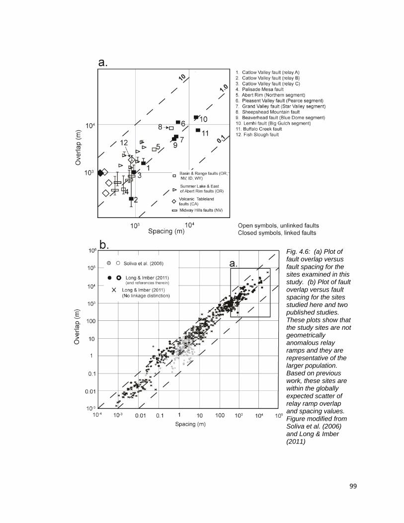
99

Fig. 4.6: (a) Plot of fault overlap versus fault spacing for the sites examined in this study. (b) Plot of fault overlap versus fault spacing for the sites studied here and two published studies. These plots show that the study sites are not geometrically anomalous relay ramps and they are representative of the larger population. Based on previous work, these sites are within the globally expected scatter of relay ramp overlap and spacing values. Figure modified from Soliva et al. (2006) and Long & Imber (2011)

100

4.5 Discussion

Fig. 4.7: Plot of outboard fault length versus relay ramp catchment area/relay ramp area (AFP/AR). High AFP/AR values indicate that a majority of the relay ramp area drains fault-parallel. Note that there appears to be a transition around 20 km which shows that fault-parallel catchments are dominant when outboard faults are less than 20 km. There is no relationship between catchment geometry and outboard fault length for sites along fault longer than about 20 km. Errors in AFP/AR

are the result of error propagation from fault length measurements.

Fig. 4.8: Plot of outboard fault length versus fault overlap/fault spacing. Results show that for outboard fault lengths of more than about 15 km, overlap/spacing ratio is less than 2. Values of overlap/spacing are unpredictable for outboard fault lengths less than 15 km. These results indicate that narrow relay ramps (overlap/spacing ratio > 2) do not tend to be present in the landscape along outboard faults. This data is interpreted to mean that narrower relays tend to breach more rapidly and therefore do not survive along larger, mature fault systems.

101

In Fig. 4.7, the most obvious feature in the data is the drastic spread of AFP/AR

values above outboard fault lengths of about 15 km. This physically means that the area

of the relay ramp that drains parallel to fault strike is the dominant fluvial network

geometry at the small scale (outboard fault length <15 km), but at the large scale

(outboard fault length >15 km) fault-transverse and fault-parallel geometries show no

scale dependence. The implication here is that there is a certain structural scale or ramp

geometry at which the draining direction for the majority of the ramp area is

unpredictable. The question is, why is there such a significant difference at the large

scale, and what does this mean for sedimentary deposition within a growing extensional

landscape?

In order to understand why AFP/AR values are so disparate at the large scale, we

first have to understand what drives the evolution of relay fluvial systems in general. In

the prevailing conceptual model, large fault-parallel catchments develop on ramp

surfaces as the faults grow and accumulate displacement (Gawthropre & Hurst, 1993).

From previous work we know that headwardly eroding catchments on outboard fault

escarpments can capture fault-parallel channels and reduce the overall ramp area that

drains toward the ramp toe (Densmore et al., 2003; Athmer & Luthi, 2011; Duffy et al.,

2014) (Fig. 4.1b & c). In essence, while not explicitly stated, earlier work has established

a mechanism (stream capture) by which relay catchment geometry may transition from a

fault-parallel dominated geometry to a fault-transverse dominated geometry. We propose

that this mechanism is the reason why AFP/AR values can become very small as outboard

fault length increases. This mechanism has been inferred for the relay fluvial system

evolution at the Blue Dome site along the Beaverhead fault, Idaho (Densmore et al.,

102

2003). The rationale is that as a given outboard fault grows in length and begins to

interact with its inboard neighbor, its displacement and displacement rate increase, which

in turn increases fluvial incision rates on the escarpment catchments. This makes capture

of the fault-parallel draining channels more likely at the larger scale (Fig. 4.1c), which

would explain the disparity in AFP/AR values. The fundamental control on whether a

scarp catchment will capture a fault-parallel channel, therefore, is the ability of the fault-

parallel channel to incise at the same rate or faster than the escarpment catchments.

Additionally, an important consideration may be the incision rate of the scarp catchments

relative to the rock uplift rate on the outboard fault. This would set the divide migration

rate on the scarp catchments and dictate if capture of a portion of AFP will occur.

Although stream capture of a fault-parallel catchment by a scarp catchment is the

mechanism by which we interpret our data, it is not the only possible mechanism.

Figures 4.9 and 4.10 show possible mechanisms by which ramp-transverse catchments

could evolve. Rather than a relay ramp catchment evolving as a fault-parallel geometry

and then transitioning to fault-transverse at a later time (as described in Fig. 4.9a & 4.10a,

Davis, 2005) for some sites the fault-transverse geometry may be the initial condition

(Fig. 4.9b & 4.10b). This is the interpreted mechanism by which relay ramp fluvial

systems evolved at the Pleasant Valley fault site (Jackson & Leeder, 1994), but it has not

been definitely shown. Regardless, our observations are still significant because they

predict which types of structural geometries would favor fault-transverse versus fault-

parallel fluvial geometries. A third possible way for fault-parallel cases to transition to a

fault-transverse geometry is shown in Fig. 4.9c & 4.10c. In this scenario, the fault-

parallel drained area has an outlet at the ramp toe, but at some point the fault tip

103

propagates passed the channel and it does not get redirected. The third scenario is the

least likely because en echelon faults do not typically propagate past one another very

much after fault initiation due to stress shadowing (Cowie, 1998; Gupta & Scholz, 2000;

Hus et al., 2005).

Fig. 4.9: Schematic map views of different scenarios in which a fault-transverse drainage may evolve. In case (a) an initially fault-parallel drainage is captured by a headwardly eroding scarp-front catchment and diverts a significant portion of the fault-parallel drained area over the outboard fault. In case (b) a fault-parallel drainage area never develops and scarp front catchments simply get larger and eventually drain the entirety of the relay ramp. In case (c) an initial fault-parallel drainage area becomes a fault-transverse drainage because the outboard fault propagates past the channel. In this case, the channel maintains flow across the fault and does not get deflected. Case (a) or case (b) seem to be likely mechanisms, however case (c), while theoretically possible, is unlikely. This unlikelihood is due to the fact that once faults attain an overlapping geometry propagation is generally arrested due to stress shadowing (Cowie, 1998).

104

Regardless of the structural and geomorphic mechanisms (capture vs. tip propagation)

responsible for channel geometry genesis or reorganization, we limit our scope to the

simple observation of over what fault scale(s) does this geomorphological transition

occur.

Future work is needed to discern which of these mechanisms is preferred or

encouraged under different scenarios (i.e., variable climate, rock type, structural

geometries, etc.). The most straightforward way to approach this is to utilize

geomorphological indicators to infer which mechanism is at work in a given scenario.

Recently, some workers have focused on the χ metric, which characterizes both the

topology and geometry of a channel network (Willett et al., 2014) and gives a measure of

the disequilibrium between adjacent watersheds. This is useful because differences in χ

Fig. 4.10: Google Earth images of three relay ramps that are interpreted to be analogous to scenarios outlined in Fig. 4.9.

105

between channel networks indicate that the drainage divide is not stable and one

watershed is in the process of capturing another. A detailed χ analysis of the sites

examined here could be useful in figuring out whether a site is one case or another (Fig.

4.9). In addition to χ, additional geomorphic indicators can be utilized to determine

which of the three mechanisms in Figs. 4.9 and 4.10 are responsible for the observed

relay channel geometry. One could examine channel profile convexities to determine if

capture has occurred (e.g., Davis, 2005). Additionally, one could examine the landscape

itself and look for evidence of abandoned/redirected channels (wind gaps) or other

features indicative of channel network reorganization. Whatever feature or metric is

utilized, they should be used in conjunction with one another to anchor any interpretation.

4.5.1 Overlap, spacing, outboard fault length and their relationship with relay ramp

shape

Recent work on relay ramp overlap and spacing relationships along en echelon

normal faults shows that the overall self-similarity of relay ramp fault overlap/spacing

ratio is demonstrable over 7-8 orders of magnitude with about 2 orders of magnitude

scatter (Soliva et al., 2006; Long & Imber, 2011; Childs et al., 2014; Fossen & Rotevatn,

2016). Indeed, our data fall within the predicted 2 orders of magnitude of scatter that is

seen in above-mentioned studies (Fig. 4.5). These studies also show that, globally, the

ratio of overlap to spacing for normal faults is somewhere between 2 and 5. Our goal

here is not to repeat previous work; rather it is important to note what previous work

omitted. One issue that cannot be readily assessed is the role of fault scale in the

overlap/spacing relationship. Previous workers have attempted to fit a power-law

106

relationship to overlap/spacing data (see Soliva et al., 2006). Although previous work

shows a self-similar relationship in overlap/spacing ratio (as discussed earlier), the scale

of the ramp bounding faults has never been included in this discussion. We posit that the

scatter in the overlap/spacing relationship can be explained by fault scale. Indeed, our

observations show that as the outboard fault gets longer the expected overlap/spacing

ratio is expected to decrease well below the global average (Fig. 4.8).

The observation that fault overlap/spacing ratio shows a scale dependency has

significant implications. For the most part, relay ramps along the largest faults that we

observe have overlap/spacing ratios of about < 2, whereas for outboard faults less than 15

km long, the ratio is highly variable. The question is, why is there relatively little scatter

in the ratio along the large faults? We know from previous work that spacing plays a

critical part in determining the degree of interaction between en echelon faults (e.g.,

Crider & Pollard, 1998; Cowie, 1998; Cowie & Roberts, 2001; Soliva et al., 2006). The

closer two en echelon faults are to one another, the greater the interaction between them,

which ultimately hastens the linking of the segments (Cowie, 1998). To put it another

way, larger spacing (for a given overlap) tends to promote longevity of the ramps, and

therefore ramp topography, in the landscape. Smaller faults (and smaller fault arrays)

would be expected to have more variable overlap/spacing ratios because they are less

mature, and hence more likely to have a wider spread of relay overlap/spacing ratios.

With time, however, as the faults and arrays grow and interact, the larger overlap/spacing

ratio relays are breached, and the outboard fault tip eventually may become inactive and

buried by hanging wall sediments, whereas lower overlap/spacing ratio ramps survive in

the landscape. Physically this makes sense because the faults along the wider relays (i.e.,

107

smaller overlap/spacing ratio) would not be expected to link as quickly as the narrower

(larger ratio) relays. If fault scale is taken into consideration, however, long (>15 km)

outboard faults appear to have overlap/spacing values biased towards about 1, because

they are the only ones that tend to resist breaching. Essentially, nature will tend to bias

the data such that relatively narrow relay ramps tend to not survive along mature

extensional faults.

The answer to the question of why overlap/spacing values are lower at larger fault

lengths may be related to the thickness of the brittle crust in the Basin and Range. The

maximum fault spacing above which faults do not interact is set by fault length and

displacement (Fossen & Rotevatn, 2016). Longer faults, therefore, can interact with one

another over larger spacing values than shorter faults can. All of the fault segments

examined here are interacting with a neighboring segment; this is evidenced by the ramp

geomorphology. In other words, the fluvial systems are obviously influenced by both

faults, not one or the other. While the relationship between fault length and maximum

interaction spacing is well defined over a broad range of scales (Fig. 4.5b, Soliva et al.,

2006; Long & Imber, 2011) there is a scale at which this relationship breaks down.

Soliva et al. (2006) show that overlapping faults that are vertically restricted have an

increasingly difficult time lengthening and propagating passed one another. Furthermore,

the faults do not link when their spacing is above a particular threshold. These

observations suggest that for relays defined by vertically restricted faults, there exists

some upper limit for overlap/spacing values at critical mechanical layer thickness and

fault length values. These observations may explain why the overlap/spacing data at

large outboard fault lengths at our study sites are skewed to less than the expected global

108

overlap/spacing value (Fig. 4.6). The largest faults we examined are large enough to cut

through the entire seismogenic thickness. This thickness controls the extent of patterns of

stress change and is likely to, therefore, control the relay geometry for the large faults.

However, this overlap/spacing-fault scale dependency is inevitably site specific because

it ultimately depends both on this layer thickness and fault length. In the Basin and

Range, seismogenic thickness is about 12-15 km (Stein & Barrientos, 1985; Doser, 1986;

Jackson & White, 1989). Note that this corresponds well to the fault length scale at

which we observe the transition in ramp catchment morphology.

4.5.2 Implications for rift basin stratigraphy and hydrocarbon exploration

This work shows that relay ramp overlap/spacing ratio and fault scale play a role

in governing geomorphological patterns in extensional basins. Previous work has

established that relay ramps are important features in terms of their impact on synrift

sedimentation (e.g., Gawthorpe & Hurst, 1993; Gupta et al., 1999) and their impact on

hydrocarbon systems (Fossen & Rotevatn, 2016, and references therein). The prevailing

conceptual model, however, is too simple because it does not consider the control

imparted by the fault geometry and how ramps evolve geomorphologically.

The results of this study show that at the smaller fault scale (< 15 km length) we

can reliably predict that more than half of the ramp area will drain parallel to fault strike

and towards the ramp toe. This indicates that early synrift sediment dispersal pathways

and depocenter locations should be predictable using the structural framework alone, at

least for smaller faults. The caveat, however, is whether there is a major axial fluvial

system that might redistribute the sedimentary deposits elsewhere in the basin. At larger

109

fault scales, interaction between initially isolated fault systems and basins could lead to a

fluctuation in base level as rifting matures from fluvial to lacustrine. Geomorphic

communication between initially isolated basins could also promote the development of

substantial axial drainage systems, which could redistribute sediment within and between

adjacent basins. Fluctuations in base level and interbasin processes illustrate the growing

complexities in predicating synrift geomorphological and sedimentological patterns at

larger fault lengths. What this means, unfortunately, and what we show here is that as

faults grow larger than 15 km in length, spatial and temporal synrift geomorphological

and sedimentation patterns are unpredictable.

These insights are valuable in regards to hydrocarbon exploration. Faulting

processes affect local rock permeability and seal potential near relay ramps; they can also

act either as fluid migration pathways or barriers to flow into overlying stratigraphic

sections. In long well-linked faults, breached relays can serve as reservoir compartments

(Fossen & Rotevatn, 2016). We have shown that the majority of relay ramps along faults

less than 15-20 km in length are expected to have sediment distribution pathways that

flow parallel to fault strike. Thus the early synrift spatial and temporal predictions of

certain hydrocarbon system variables (especially those related to source or reservoir) can

be made if certain information about the structural geometry is known.

4.6 Conclusion

The observations made in this work show that relay ramp catchment geometry is

associated with specific geometries of the ramp bounding faults. We show that there is a

predictable relationship between relay catchment geometry and fault scale when the

110

outboard fault is less than about 15-20 km long. This relationship, however, breaks down

at longer OFLs. We also show that fault O/S ratio exhibits scale dependence. Our

observations demonstrate that relays along outboard faults greater than about 20 km in

length are only associated with O/S ratios of less than 2. For relays along outboard faults

less than 15 km in length, O/S ratios fall between 1 and 5. These results suggest that

relay ramps are favored to persist in the landscape adjacent to long faults when O/S ratio

is sufficiently low, such that linkage between segments is inhibited. Thus, the relay

topography is preserved in the landscape along longer faults but only at smaller O/S

ratios. Larger O/S ratio relay ramps, however, are less likely to persist, which explains

why they are abundant along smaller, less mature fault systems. These observations are

significant because they allow us to make more reliable predictions of synrift sediment

transport systems, which impact the understanding of extensional landscapes in

continental rifts and synrift hydrocarbon systems. In other words, we can use the

geomorphological relationships observed here in relation to the structural geometry (at

least near shorter faults) to predict early synrift depositional patterns. Our observations,

and the relationships we have noted throughout this work, however, are most applicable

to the early synrift phase.

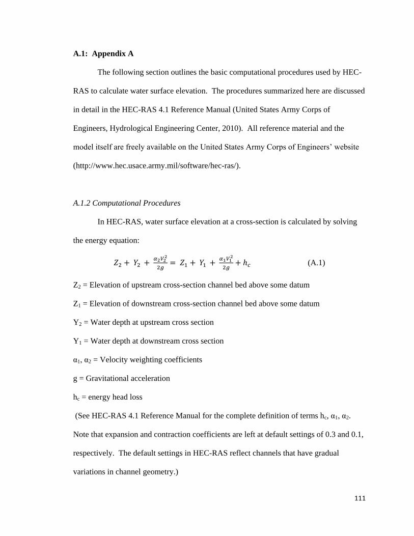
111

A.1: Appendix A

The following section outlines the basic computational procedures used by HEC-

RAS to calculate water surface elevation. The procedures summarized here are discussed

in detail in the HEC-RAS 4.1 Reference Manual (United States Army Corps of

Engineers, Hydrological Engineering Center, 2010). All reference material and the

model itself are freely available on the United States Army Corps of Engineers’ website

(http://www.hec.usace.army.mil/software/hec-ras/).

A.1.2 Computational Procedures

In HEC-RAS, water surface elevation at a cross-section is calculated by solving

the energy equation:

𝑍2 + 𝑌2 + 𝛼2𝑉2

2

2𝑔= 𝑍1 + 𝑌1 +

𝛼1𝑉12

2𝑔+ ℎ𝑐 (A.1)

Z2 = Elevation of upstream cross-section channel bed above some datum

Z1 = Elevation of downstream cross-section channel bed above some datum

Y2 = Water depth at upstream cross section

Y1 = Water depth at downstream cross section

α1, α2 = Velocity weighting coefficients

g = Gravitational acceleration

hc = energy head loss

(See HEC-RAS 4.1 Reference Manual for the complete definition of terms hc, α1, α2.

Note that expansion and contraction coefficients are left at default settings of 0.3 and 0.1,

respectively. The default settings in HEC-RAS reflect channels that have gradual

variations in channel geometry.)

112

In order to start the procedure to solve for Y2, HEC-RAS requires an initial downstream

water depth, Y1, which in our case is given as normal depth (flow is uniform and steady;

see Table 1 for other parameters used). HEC-RAS uses an iterative procedure where

water surface elevation is determined by balancing the energy equation. HEC-RAS uses

the normal depth condition to calculate a water depth at the most downstream cross-

section and uses this depth to compute water depth at the next upstream cross-section. In

order to balance the energy equation, HEC-RAS first approximates an upstream water

depth using the water depth calculated at the cross-section just downstream. HEC-RAS

assumes the water depth, but if the model cannot balance the energy equation within 20

iterations, the program issues a warning indicating it cannot balance the equation in the

subcritical regime and flags the cross-section. If mixed flow regime is selected (as in our

models), HEC-RAS returns to those cross sections and calculates the water depth using

the momentum equation, given by:

𝑄22𝛽2

𝑔𝐴2+ 𝐴2𝑌2 + (

𝐴1+𝐴2

2) 𝐿𝑆0 − (

𝐴1+𝐴2

2) 𝐿𝑆𝑓 =

𝑄12𝛽1

𝑔𝐴1+ 𝐴1𝑌1 (A.2)

Q2 = upstream discharge

Q1 = downstream discharge

β1,2 = momentum coefficient

A2 = wetted cross-sectional area of upstream cross-section

A1 = wetter cross-sectional area of downstream cross-section

𝑌1 = depth from water surface to centroid of cross-sectional area (downstream cross

section)

𝑌2= depth from water surface to centroid of cross-sectional area (upstream cross section)

L = distance between cross-sections

113

S0 = channel slope

𝑆𝑓 = friction slope

(See HEC-RAS 4.1 Reference Manual for complete definitions of terms).

In channels where the geometry changes rapidly (i.e., sudden changes in slope) the

momentum equation is used to calculate water depth. Because the energy equation is

only considered valid in gradually varied flows, HEC-RAS uses the momentum equation

to solve for water depth when the energy equation returns a water surface elevation at

critical depth. In the case of our study channels, by using the momentum equation to

calculate water depth, HEC-RAS has made the assumption that a hydraulic jump exists

between cross sections.

A.1.3 Model parameters

In order to run a model flow in HEC-RAS certain parameters must be defined or

given a numerical value. Table A.1 shows the parameters used.

Full

Discharge

(m3/s)

Half

Discharge

(m3/s)

Manning’s

n

Boundary

Condition

Flow

Regime

Unlinked

Faults

0.4 0.2 0.0445 Normal

Depth

Mixed

Partially

Breached

Ramp 1

0.15 0.075 0.0675 Normal

Depth

Mixed

Partially

Breached

Ramp 2

0.3 0.15 0.0675 Normal

Depth

Mixed

Fully

Breached

Ramp

0.15 0.075 0.0675 Normal

Depth

Mixed

Table A.1: List of parameters used in HEC-RAS models.

114

We set discharge for the channels by trial and error, as we have no data on discharge.

First, a discharge of about 1.0 m3/s is routed through the system and every cross-section

is inspected. If any cross-section overflows (i.e., any water is present outside of the

cross-section), then discharge is reduced by 0.1 m3/s and the procedure continues until a

discharge is reached that produces no overfilling. We define the largest discharge that

results in no overfilling as ‘full’ discharge. Once a ‘full’ discharge is determined, the

model is run and the values of channel width, water depth and bed shear stress are

extracted and saved. It should be noted that discharge does not change through the

channel reach. Next, the ‘full’ discharge for each channel is halved and the ‘half’

discharge is used to complete a second model run. Channel width, water depth and bed

shear stress values are extracted and saved from the half discharge model run.

In order to see how changes in discharge affect channel width, water depth and

bed shear stress, we show the range of values between full and half discharge. First, the

average values of width, depth and shear stress are calculated and plotted. The

differences between the average and full and half discharge are then plotted as vertical

bars, which denote the variability in values between model runs.

Figures 2.7, 2.8, and 2.9 show the results of the HEC-RAS models. We do not

know how discharge would vary in the real world along each channel reach so we choose

a single discharge to be run for the entire length of the system. With this in mind, the

utility of this analysis is obvious because we can examine how geometry changes through

a channel reach. We take this simplistic approach because we lack the appropriate

information to make discharge variations at each cross section. More specifically, we

115

lack detailed topographic data to make a determination of how much drainage area lies

upstream of a given cross-section.

We determine Manning’s roughness for each field site using guidelines set by the

U.S. Geological Survey (Arcement & Schneider, 1989). While roughness coefficients

were likely different when the channels were active in the past (i.e., changes in

vegetation), our values approximate general channel conditions (e.g., bed material and

channel planform) that have probably not changed very much. We set upstream and

downstream boundary conditions at normal depth, which is defined as the depth when

flow is uniform. In the absence of hydrological data, HEC-RAS limits the boundary

conditions to either normal depth or critical depth. In this case it is unrealistic to choose

critical depth. While we make the simplifying assumption that flow is steady and

uniform at the model endpoints (by assuming normal depth boundary condition), this

assumption is more justifiable. We cannot justify the use of critical depth here because

we observe no features, such as knickpoints, in our channels near the endpoints that

would suggest flow would be critical. An additional consideration we must make is

whether the flow regime is supercritical, subcritical, or mixed. Because we see evidence

of both in our channels (i.e., supercritical at knickpoints or knickzones and subcritical

between knickpoints), we chose mixed flow. The decision to use mixed flow is best in

the case of our study channels, because it gives HEC-RAS the latitude to make more

realistic determinations of water surface elevation.

We specifically do not consider width, depth and bed shear stress data points at

the model endpoints (the first and last cross-sections), because these data contain our

chosen boundary conditions. For this reason, the first and last cross-section in each

116

channel is not shown in the data set. The removed data points translate to about 50 m

from both the upstream and downstream ends of each channel.

117

B.1: Appendix B

This appendix is a compendium of field maps for the 27 sites examined in chapter

4. Each site map contains the mapped fault traces that form the relay ramp, an AR

polygon, an AFP polygon, a spacing line and an overlap line (see Methods section). The

site maps were made using Digital Orthophoto Quarter Quadrangles (DOQQs) and a 10

m digital elevation model (DEM). The surfaces shown in all of the maps are from the

DOQQs. All mapping was performed in ArcGIS v. 10.0. Values obtained for each of

these variables are collated in Table 4.1.

Fig. B1: Site maps of Volcanic Tableland relay ramps.

118

Fig. B2: Site maps of Midway Hills relay ramps.

119

Fig. B3: Site maps of Palisade Mesa, Pearce and Buffalo Creek relay ramps.

120

Fig. B4: Site maps of Big Gulch (Lemhi fault), Blue Dome (Beaverhead fault) and Star Valley (Grand Valley fault) relay ramps.

121

Fig. B5: Site maps of east of Abert Rim and Sheepshead Mountain relay ramps.

122

Fig. B6: Site maps of Catlow Valley relays (A,B,C), Abert Rim and east of Summer Lake relay ramps.

123

Bibliography

ADAMS, K. D., & WESNOUSKY, S. G. (1998) Shoreline processes and the age of the Lake

Lahontan highstand in the Jessup embayment, Nevada. Geol. Soc. Am. Bull., 110,

1318-1332.

AMOS, C.B. & BURBANK, D.W. (2007) Channel width response to differential uplift. J.

Geophys. Res., 112. F02010, doi: 10.1029/2006JF000672.

ANDERSON, R.S. & MENKING, K.M. (1994) The Quaternary marine terraces of Santa Cruz,

California: Evidence for coseismic uplift on two faults. GSA Bull., 106, 649-664.

ARCEMENT, G.J., & SCHNEIDER, V.R. (1989) Guide for selecting manning's roughness

coefficients for natural channels and flood plains. U.S. Geol.Surv. Water-Supply

Pap. 2339, U.S. Geological Survey. Reston, VA.

ATHMER, W. & LUTHI, S.M. (2011) The effect of relay ramps on sediment routes and

deposition: A review. Sed. Geology, 242, 1-17.

ATTAL, M., TUCKER, G.E., WHITTAKER, A.C., COWIE, P.A., & ROBERTS, G.P. (2008)

Modeling fluvial incision and transient landscape evolution: Influence of dynamic

channel adjustment. J. Geophys. Res., 113, F03013, doi: 10.1029/2007Jf000893

ATWOOD, G. (1994) Geomorphology applied to flooding problems of closed-basin

lakes…specifically Great Salt Lake, Utah. Geomorphology, 10, 197-219.

BATEMAN, P.C. (1965) Geology and tungsten mineralization of the Bishop District, CA,

U.S. Geol. Surv. Prof. Pap., 470 Reston, VA.

BONNET, E., BOUR, O., ODLING, N.E., DAVY, P., MAIN, I., COWIE, P. & BERKOWITZ, B.

(2001) Scaling of fracture systems in geological media. Reviews of Geophysics,

39, 347-383.

124

BURBANK, D.W. & ANDERSON, R.S. (2011) Tectonic Geomorphology, 2nd

Edition.

Blackwell Science, 274 pp.

CARTER, D.T., ELY, L.L., O’CONNOR, J.E. & FENTON, C.R. (2006) Late Pleistocene

outburst flooding from pluvial Lake Alvord into the Owyhee River, Oregon.

Geomorphology, 75, 346-367.

CARTWRIGHT, J.A., TRUDGILL, B.D. & MANSFIELD, C.S. (1995) Fault growth by segment

linkage: An explanation for scatter in maximum displacement and trace length

data from the Canyonlands grabens of SE Utah. J. Struct. Geol., 17, 1319-1326.

CARTWRIGHT, J.A., MANSFIELD, C. & TRUDGILL, B. (1996) The growth of normal faults by

segment linkage. from Buchanan, P.G. & Nieuwland, D.A. (eds), 1996) Modern

Developments in Structural Interpretation, Validation and Modelling, Geological

Society Special Publication No. 99, 163-177.

CHILDS, C., WATTERSON, J. & WALSH, J.J. (1995) Fault overlap zones within developing

normal fault systems. J. Geol. Society, 152, 535-549.

CHILDS, C., CONNEALLY, J., DELOGKOS, E., MANZOCCHI, T., NICOL, A., AISLING, S., &

WALSH, J. (2014) A relationship between relay ramp aspect ratio and normal drag:

abstract in Geometry and Growth of Normal Faults, Geol. Soc. London, 101-102.

CHOI, S.J., MERRITTS, D.J. & OTA, Y. (2008) Elevations and ages of marine terraces and

late Quaternary rock uplift in southeastern Korea. J. Geophys. Res., 113, B10403,

doi:10.1029/2007JB005260.

COMMINS, D., GUPTA, S. & CARTWRIGHT, J. (2005) Deformed streams reveal growth and

linkage of a normal fault array in the Canyonlands graben, Utah. Geology, 33,

645-648.

125

COWIE, P.A. & SCHOLZ, C.H. (1992) Physical explanation for the displacement-length

relationship of faults using a post-yield fracture mechanics model. J. Struct. Geol.,

14, 1133-1148.

COWIE, P.A. (1998) A healing-reloading feedback control on the growth rate of

seismogenic faults. J. Struct. Geol., 20, 1075-1087.

COWIE, P.A., GUPTA, S., & DAWERS, N.H. (2000) Implications of fault array evolution for

synrift depocentre development: Insights from a numerical fault growth model.

Basin Res., 12, 241-261.

COWIE, P. & ROBERTS, G.P. (2001) Constraining slip rates and spacings for active normal

faults: J. Struct. Geol., 23, 1901-1915.

COWIE, P.A., ATTAL, M., TUCKER, G.E., WHITTAKER, A.C., NAYLOR, M., GANAS, A. &

ROBERTS, G.P. (2006) Investigation of the surface process response to fault

interaction and linkage using a numerical modeling approach. Basin Res., 18,

231-266.

CRIDER, J.G. (2001) Oblique slip and the geometry of normal-fault linkage: mechanics

and a case study from the Basin and Range in Oregon: J. Struct. Geol., 23, 1997-

2009

CRIDER, J.G. & POLLARD, D.D. (1998) Fault linkage: three-dimensional mechanical

interaction between echelon normal faults: J. Geophys. Res., 103, 24373-24391.

CRONE, A.J. & MACHETTE, M.N. (1984) Surface faulting accompanying the Borah Peak

earthquake, central Idaho: Geology, 12, 664-667.

126

EVANS, J.G. & GEISLER, T.M. (2001) Geologic field-trip guide to Steens Mountain Loop

Road, Harney County, Oregon. U.S. Geol. Surv, Bureau of Land Management

Bull. 2183.

DAVIS, A.M. (2005) Geomorphological evolution of propagating fault tips in extensional

and compressional settings. Unpublished PhD thesis. Imperial College London,

United Kingdom

DAWERS, N.H., ANDERS, M.H. & SCHOLZ, C.H. (1993) Growth of normal faults:

displacement -length scaling. Geology, 21, 1107-1110.

DAWERS, N.H. & ANDERS, M.H. (1995) Displacement-length scaling and fault linkage. J.

Struct. Geol., 17, 607-614.

DAWERS, N.H., & UNDERHILL, J.R. (2000) The role of fault interaction and linkage in

controlling synrift stratigraphic sequences: Late Jurassic, Stratfjord East Area,

Northern North Sea. Am. Asso. of Petrol. Geo. Bull., 84, 45-64.

DENSMORE, A.L., DAWERS, N.H., GUPTA, S., ALLEN, P.A. & GILPIN, R. (2003) Landscape

evolution at extensional relay zones. J. Geophy. Res., 108, B5, doi:

10.1029/2001JB001741.

DENSMORE, A.L., DAWERS, N.H., GUPTA, S., GUIDON, R. & GOLDIN, T. (2004) Footwall

topographic development during continental extension. J. Geophy. Res., 109, doi:

10.1029/2003JF000115.

DIGGLES, M.F., CONRAD, J.E. & SOREGHAN, G.A. (1990) Geologic map of the Diablo

Mountain Wilderness Study Area, Oregon, U.S. Geol. Survey Map MF-2121,

scale 1:48,000.

127

DIXON, T.H., NORABUENA, E. & HOTALING, L. (2003) Paleoseismology and global

positioning system: earthquake-cycle effects and geodetic versus geologic fault

slip rates in the Eastern California Shear Zone. Geology, 31, 55-58.

DOHRENWEND, J.C., SCHELL, B.A., MENGES, C.M., MORING, B.C. & McKITTRICK, M.A.

(1996) Reconnaissance photogeologic map of young (Quaternary and late

Tertiary) faults in Nevada, in Analysis of Nevada’s metal-bearing mineral

resources: D.A. Singer (ed) Nevada Bureau of Mines and Geology Open-File

Report 96-2, 1 pl., scale 1:1,000,000.

DOHRENWEND, J.C., SCHELL, B.A. & MORING, B.C. (1992) Reconnaissance photogeologic

map of young faults in the Millett 1° by 2° quadrangle, Nevada: U.S. Geol. Survey

Miscellaneous Field Studies Map MF-2176, 1 sheet, scale 1:250,000.

DOKKA, R.K. & TRAVIS, C.J. (1990a) Late Cenozoic strike-slip faulting in the Mojave

Desert, California. Tectonics, 9, 311-340.

DOKKA, R.K. & TRAVIS, C.J. (1990b) Role of the eastern California shear zone in

accommodating Pacific-North American plate motion. Geophys. Res. Lett., 17,

1323-1326.

DOSER, D.I. (1986) Earthquake processes in the Rainbow Mountain-Fairview Peak-Dixie

Valley, Nevada region 1954-1959. J. Geophys. Res. 91, 12572-12586.

DUFFY, O.B., BROCKLEHURST, S.H., GAWTHORPE, R.L., LEEDER, E.L. & FINCH, E. (2015)

Controls on landscape and drainage evolution in regions of distributed normal

faulting: Perachora Peninsula, Corinth Rift, Central Greece: Basin Res., 27, 473-

494.

128

DUVALL, A., KIRBY, E. & BURBANK, D. (2004) Tectonic and lithologic controls on

bedrock channel profiles and processes in coastal California. J. Geophys. Res.,

109, F03002, doi: 10.1029/2003JF000086.

FERRILL, D.A., STAMATAKOS, J.A. & SIMS, D. (1999) Normal fault corrugation:

Implications for growth and seismicity of active normal faults. J. Struct. Geol.,

21, 1027-1038.

FERRILL, D.A. & MORRIS, A.P. (2001) Displacement gradient and deformation in normal

fault systems: J. Structural Geol., 23, 619-638.

FINNEGAN, N.J., ROE, G., MONTCOMERY, D.R., & HALLET, B. (2005) Controls on the

channel width of rivers: Implications for modeling fluvial incision of bedrock:

Geology, 33, 229-232.

FOSSEN, H. & ROTEVATN, A. (2016) Fault linkage and relay structures in extensional

settings – a review. Earth Science Reviews, doi: 10.1016/j.earscirev.2015.11.014.

GAWTHORPE, R.L. & HURST, J.M. (1993) Transfer zones in extensional basins: their

structural style and influence on drainage development and stratigraphy. J. Geol.

Soc. London, 150, 1137-1152.

GAWTHORPE, R.L. & LEEDER, M.R. (2000) Tectono-sedimentary evolution of active

extensional basins. Basin Res., 12, 195-218.

GESCH, D.B., OIMOEN, M.J. & EVANS, G.A. (2014) Accuracy assessment of the U.S.

Geological Survey National Elevation Dataset, and comparison with other large-

area elevation datasets – SRTM and ASTER. U.S. Geol. Surv. Open-File Report

2014-1008.

129

GILBERT, G.K. (1877) Geology of the Henry Mountains, U.S. Geol. Surv. Report, pp.

160.

GILBERT, C.M. (1938) Welded tuff in eastern California. Geol. Soc. Am. Bull., 49, 1829-

1862.

GILPIN, R. (2003) Interaction between stream development and propagating extensional

faults. Unpublished PhD Thesis, University of Edinburgh, Scotland.

GOETHALS, M.M., NIEDERMANN, S., HETZEL, R. & FENTON, C.R. (2009) Determining the

impact of faulting on the rate of erosion in a low-relief landscape: A case study

using in situ produced 21

Ne on active normal faults in the Bishop Tuff, California.

Geomorphology, 103, 401-413.

GUPTA, S., COWIE, P.A., DAWERS, N.H. & UNDERHILL, J.R. (1998) A mechanism to

explain rift-basin subsidence and stratigraphic patterns through fault-array

evolution. Geology, 26, 595-598.

GUPTA, S., UNDERHILL, J.R., SHARP, I. & GAWTHORPE, R.L. (1999) Role of fault

interactions in controlling synrift sediment dispersal patterns: Miocene, Abu

Alaqa Group, Suez Rift, Sinai, Egypt. Basin Res., 11, 167-189.

GUPTA, A. & SCHOLZ, C.H. (2000) A model of normal fault interaction based on

observation and theory. J. Structural Geol., 22, 865-879.

HACK, J.T. (1957) Studies of longitudinal stream profiles in Virginia and Maryland. U.S.

Geol. Surv. Prof. Pap., 294-B, Reston, VA.

HARE, L., FERGUSON, J. F., AIKEN, C. L. V. & OLDOW, J. S. (2001) Quantitative

characterization and elevation estimation of Lake Lahontan shoreline terraces

130

from high-resolution digital elevation models. J. Geophys. Res., 106, B11,

26761-26774.

HODGKINSON, K.M., STEIN, R.S. & KING, G.C.P. (1996) The 1954 Rainbow Mountain-

Fairview Peak- Dixie Valley earthquakes: A triggered normal faulting sequence.

J. Geophys. Res.,101, 25459-25471.

HOOPER, P. R., BINGER, G. B. & LEES, K. R. (2002) Ages of the Steens and Columbia

River flood basalts and their relationship to extension-related calc-alkalic

volcanism in eastern Oregon. GSA Bul., 114, 43-50.

HOPKINS, M.C. & DAWERS, N.H. (2015) Changes in bedrock channel morphology driven

by displacement rate increase during normal fault interaction and linkage. Basin

Res., 27, 43-59.

HUS, R., ACOELLA, V., FUNICIELLO, R., & DE BATIST, M. (2005) Sandbox models of relay

ramp structure and evolution. J. Struct. Geol., 27, 549-473.

IBARRA, D.E., EGGER, A.E., WEAVER, K.L., HARRIS, C.R. & MAHER, K. (2014) Rise and

fall of late Pleistocene pluvial lakes in response to reduced evaporation and

precipitation: Evidence from Lake Surprise, California. GSA Bull., 126, 1387-

1415.

IMBER, J., TUCKWELL, G.W., CHILDS, C., WALSH, J.J., MANZOCCHI, T., HEATH, A.E.,

BONSON, C.G. & STRAND, J. (2004) Three-dimensional distinct element modelling

of relay growth and breaching along normal faults. J. Struct. Geol., 26, 1897-

1911.

JACKSON, J. & LEEDER, M. (1994) Drainage systems and the development of normal

faults: an example from Pleasant Valley, Nevada: J. Struct. Geol., 16, 1041-1059.

131

JACKSON, J.A. & WHITE, N.J. (1989) Normal faulting in the upper continental crust:

observations from regions of active extension. J. Struct. Geol., 11, 15-36.

KIRBY, E., & WHIPPLE, K. X. (2012) Expression of active tectonics in erosional landscapes.

J. Struct. Geol., 44, 54-75.

LICCIARDI, J.M. (2001) Chronology of latest Pleistocene lake-level fluctuations in the

pluvial Lake Chewaucan basin, Oregon, USA. J. Quat. Sci., 16, 545-553.

LIDKE, D.J. (compiler) (2000) Fault number 1192, Buffalo Creek fault zone, in

Quaternary fault and fold database of the United States: U.S. Geol. Surv. website,

<http://earthquakes.usgs.gov/hazards/qfaults>

LIENKAEMPER, J.J., PEZZOPANE, S.K., CLARK, M.M., & RYMER, M.J. (1987) Fault

fractures formed in association with the 1986 Chalfant Valley, California,

earthquake sequence: Preliminary report. Bull. Seismol. Soc. Am., 77, 297-305.

LOCKE, W. W. & MEYER, G.A. (1994) A 12,000-year record of vertical deformation

across the Yellowstone caldera margin: The shorelines of Yellowstone Lake. J.

Geophys. Res., 99, B10, 20079-20094.

LONG, J.J. & IMBER, J. (2011) Geological controls on fault relay zone scaling: J. Struct.

Geol., 33, 1790-1800.

LUDINGTON, S., MORING, B.C., FLYNN, K.S. & HOPKINS, M.J. (2005) Preliminary

integrated databases for the United States – western states: California, Nevada,

Arizona, and Washington. U.S. Geological Survey Open File Report2005-1305.

McCALPIN, J.P., MACHETTE, M.N. & HALLER, K.M. (compilers) (2011) Fault number

726d, Grand Valley fault, Star Valley section, in Quaternary fault and fold

132

database of the United States: U.S. Geological Surv. website,

<http://earthquakes.usgs.gov/hazards/qfaults>

McLEOD, A.E., UNDERHILL, J.R., DAVIES, S.J. & DAWERS, N.H. (2002) The influence of

fault array evolution on synrift sedimentation patterns: Controls on deposition in

the Strathspey-Brent-Statfjord half graben, northern North Sea: AAPG Bull., 86,

1061-1093.

MERRITTS, D.J. & BULL, W.B. (1989) Interpreting Quaternary uplift rates at the

Mendocino triple junction, northern California, from uplifted marine terraces.

Geology, 17, 1020-1024.

MILLER, M.M., JOHNSON, D.J., DIXON, T.H. & DOKKA, R.K. (2001) Refined kinematics of

the Eastern California Shear Zone from GPS observations, 1993-1998. J.

Geophys. Res., 103, 2245-2263.

NEGRINI, R.M. (2002) Pluvial lake sizes in the northwestern Great Basin throughout the

Quaternary period. in Great Basin Aquatic Systems History, Hershler, R., Madsen

D.B., & Currey D.R, (eds). Smithsonian Contributions to the Earth Sciences No.

33, Smithsonian Press; Washington, DC.

O’CONNEL, J.F. & INOWAY, C.M. (1994) Surprise Valley projectile points and their

chronological implications. J. Calif. Great Basin Anthro., 16, 162.198.

OLDOW, J. S. & SINGLETON, E. S. (2008) Application of Terrestrial Laser Scanning in

determining the pattern of late Pleistocene and Holocene fault displacement from

the offset of pluvial lake shorelines in the Alvord extensional basin, northern

Great Basin, USA. Geosphere, 4, 536-563.

133

PEACOCK, D.C.P., & SANDERSON, D.J. (1991) Displacements, segment linkage and relay

ramps in normal fault zones. J. Struct. Geol., 13, 721-733.

PEACOCK, D.C.P. & SANDERSON, D.J. (1994) Geometry and development of relay ramps

in normal fault systems. AAPG Bull., 78, 147-165.

PERSONIUS, S.F. (compiler) (2002) Fault number 1800, Unnamed Sheepshead Mountains

fault, in Quaternary fault and fold database of the United States: U.S. Geol. Surv.

website, <http://earthquakes.usgs.gov/hazards/qfaults>

PEZZOPANE, S.K. & WELDON II, R.J. (1993) Tectonic role of active faulting in central

Oregon. Tectonics, 12, 1140-1169.

PHILLIPS, J.D. & LUTZ, J.D. (2008) Profile convexities in bedrock and alluvial streams.

Geomorphology, 102, 554-566.

PIETY, L.A., SULLIVAN, T.J. & ANDERS, M.H. (1992) Segmentation and paleoseismicity of

the Grand Valley fault, southeastern Idaho and western Wyoming. in Regional

geology of eastern Idaho and western Wyoming (eds) Paul Link, Mel Kuntz &

Lucian Platt, Geol. Society Am. Memoir, 179, 155-182.

PINTER, N. (1995) Faulting on the Volcanic Tableland, Owens Valley, California. J.

Geol., 103, 73-83.

PINTER, N. & KELLER, E.A. (1995) Geomorphological analysis of neotectonic

deformation, northern Owens Valley, California. Geol. Rund., 84, 200-212.

PINTER, N., KELLER, E.A., & WEST, R.B. (1994) Relative dating of terraces of the Owens

River, Northern Owens Valley, California, and correlation with moraines of the

Sierra Nevada. Quat. Res., 42, 266-276.

134

REED, S.L., LINK, P.K., STANFORD, L.R. & LONG, S.P. (2012) Geologic Map of Idaho,

Idaho Geological Surv., scale 1:750,000.

REHEIS, M.C., 1999. Extent of Pleistocene lakes in the western Great Basin. U.S. Geol.

Surv. Miscellaneous Field Studies Map MF-2323, scale 1:800,000.

Survey Miscellaneous Field Studies Map MF-2323, scale 1:800,000.

REHEIS, M.C., ADAMS, K.D., OVIATT, C.G. & BACON, S.N. (2014) Pluvial lakes in the

Great Basin of the western United States – a view from the outcrop. Quat. Sci.

Rev., 97, 33-57.

SARNA-WOJCICKI, A.M., PRINGLE, M.S. & WIJBRANS, J. (2000) New 40

Ar/39

Ar Age of the

Bishop Tuff from multiple sites and sediment rate calibration for the Matuyama-

Brunhes boundary. J. Geophys. Res., 105, 21431-21443.

SAWYER,T.L.(compiler) (1998) Fault number 1342, Midway Hills fault, in Quaternary

fault and fold database of the United States: U.S. Geol. Surv.

<http://earthquake.usgs.gov/hazards/qfaults>.

SCARBERRY, K. C., MEIGS, A. J. & GRUNDER, A. L. (2010) Faulting in a propagating

continental rift: Insight from the late Miocene structural development of the Abert

Rim fault, southern Oregon, USA. Tectonophysics, 488, 71-86.

SCHELL, B.A. (1981) Faults and lineaments in the MX Sitting Region, Nevada and Utah,

Volume I: Technical report to U.S. Department of [Defense] the Air Force,

Norton Air Force Base, California, under Contract FO4704-80-C-0006,

November 6, 1981, 77 p.

135

SCOTT, A.T. & PINTER, N. (2003) Extraction of coastal terraces and shoreline-angle

elevations from digital terrain models, Santa Cruz and Anacapa Islands,

California. Phys. Geography, 24, 271-294.

SOLIVA, R., BENEDICTO, A. & MAERTEN, L. ( 2006) Spacing and linkage of confined

normal faults: Importance of mechanical thickness: J. Geophys. Res., 111, doi:

10.1029/2004JB003507.

STEIN, R.S. & BARRIENTOS, S.E. (1985) Planar high-angle faulting in the Basin and

Range: geodetic analysis of the 1983 Borah Peak, Idaho, earthquake. J. Geophys.

Res., 90, 11355-11366.

TOPAL, S., KELLER, E., BUFE, A. & KOCYIGIT, A. (2016) Tectonic geomorphology of a

large normal fault: Aksehir fault, SW Turkey. Geomorphology. doi:

10.1016/j.geomorph.2016.01.014.

TRUDGILL, B. & CARTWRIGHT, J. (1994) Relay-ramp forms and normal-fault linkage,

Canyonlands National Park, Utah. Geol. Soc. Am. Bull., 106, 1143-1157.

TUROWSKI, J.M., LAGUE, D., CRAVE, A., & HOVIUS, N. (2006) Experimental channel

response to tectonic uplift. J. Geophys. Res., 111, doi: 10.1029/2005JF000306.

TUROWSKI, J.M., LAGUE, D., & HOVIUS, N. (2007) Cover effect in bedrock abrasion: A

new derivation and its implications for the modeling of bedrock channel

morphology. J. Geophys. Res., 112, doi: 10.1029/2006JF000697.

UNITED STATES ARMY CORPS OF ENGINEERS, HYDROLOGIC ENGINEERING CENTER (2010)

HEC-RAS River Analysis System: User’s Manual, Applications Guide, Hydraulic

Reference Manual. United States Army Corps of Engineers: Institute for Water

136

Resources, Davis, CA. http://www.hec.usace.army.mil/software/hec-ras/hecras-

document.html

VANDER MEULEN, D. B., GRISCOM, A., KING, H. D., VERCOUTERE, T. L. & MOYLE, P.R.

(1988) Mineral Resources of the Home Creek Wilderness Study Area Harney

County, Oregon. U.S. Geol. Surv. Bulletin 1740-C.

WALLACE, R.E. (1984) Fault scarps formed during the earthquakes of October 2, 1915 in

Pleasant Valley, Nevada, and some tectonic implications. Prof. Pap. U.S. Geol.

Surv. 1274A, 1-33.

WALKER, G.W. & MACLEOD, N.S. (1991) Geologic map of Oregon: U.S. Geol. Surv.,

scale 1:500,000.

WELDON, R.J., FLETCHER, D.K., WELDON, E.M., SCHARER, K.M. & McCRORY, P.A. (2002)

An update of Quaternary faults of central and eastern Oregon: U.S. Geol. Surv.

Open-File Report 02-301.

WHIPPLE, K.X. (2004) Bedrock rivers and the geomorphology of active orogens. Ann.

Rev. Earth and Planet. Sci., 32, 151-185.

WHITTAKER, A.C., COWIE, P.A., ATTAL, M., TUCKER, G.E. & ROBERTS, G.P. (2007a)

Bedrock channel adjustment to tectonic forcing: Implications for predicting river

incision rates. Geology, 35, 103-106.

WHITTAKER, A.C., COWIE, P.A., ATTAL, M., TUCKER, G.E., & ROBERTS, G.P. (2007b)

Contrasting transient and steady-state rivers crossing active normal faults: New

field observations from the central Apennines, Italy. Basin Res., 19, 529-556.

137

WHITTAKER, A.C., ATTAL, M., COWIE, P.A., TUCKER, G.E. & ROBERTS, G.P. (2008)

Decoding temporal and spatial patterns of fault uplift using transient river long

profiles. Geomorphology, 100, 506-526.

WHITTAKER, A.C. & WALKER, S.A. (2015) Geomorphic constraints on fault throw rates

and linkage times: Examples from the Northern Gulf of Evia, Greece. J.

Geophys. Res. Earth Surface. 120, 137-158.

WILLDEN, R. & SPEED, R.C. (1974) Geology and mineral deposits of Churchill County,

Nevada: Nevada Bureau of Mines and Geology Bulletin 83, 95 p.

WILLEMSE, E.J.M., POLLARD, D.D. & AYDIN, A. (1996) Three-dimensional analyses of

slip distributions on normal fault arrays with consequences for fault scaling. J.

Struct. Geol., 18, 295-309.

WILLEMSE, E.J.M. (1997) Segmented normal faults: Correspondence between three-

dimensional mechanical models and field data. J. Geophys. Res – Solid Earth,

102, 675-692.

WILLETT, S.D., MCCOY, S.W., PERRON, J.T., GOREN, L. & CHEN, C. (2014) Dynamic

reorganization of river basins. Science, 343, 1117-1126

WILSON, C.J.N., & HILDRETH, W. (1997) The Bishop Tuff: New insights from eruptive

stratigraphy. J. Geol., 105, 407-439.

WOBUS, C.W., TUCKER, G.E., & ANDERSON, R.S. (2006) Self-formed bedrock channels.

Geophys. Res. Lett., 33, doi: 10.1029/2006GL027182.

YANITES, B.J. & TUCKER, G.E. (2010) Controls and limits on bedrock channel geometry.

J. Geophys. Res., 115, F04019, doi: 10.1029/2009JF001601.

138

YILDIRIM, C., MELNICK, D., BALLATO, P., SCHILDGEN, T.F., ECHTLER, H., ERGINAL, A.E.,

GÜNEC KIYAK, N. & STRECKER, M.R. (2013) Differential uplift along the northern

margin of the Central Anatolian Plateau: inferences from marine terraces. Quart.

Sci. Rev., 81, 12-28.

139

Biography

Michael C. Hopkins was born May 2, 1986 in Biloxi, Mississippi. He is the youngest of

three children. His parents are Michael T. Hopkins and Trudy A. Landry, both are

natives of Biloxi. He graduated from Biloxi High School in 2004. Following high

school, he attended Mississippi Gulf Coast Community College for two years (2004-

2006) and spent one year at the University of South Alabama (2006-2007) before earning

a BS in geology from the University of Southern Mississippi in 2010. In 2010, he started

graduate work at Tulane University under Nancye H. Dawers and completed this Ph.D.

dissertation in 2016.