geometry optimization - university of york
TRANSCRIPT
Geometry OptimizationMatt ProbertCondensed Matter Dynamics GroupDepartment of Physics, University of York, U.K.http://www-users.york.ac.uk/~mijp1

Overview of lecture
n Background Theoryn Hellman-Feynman theoremn BFGS and other algorithms
n CASTEP detailsn Useful keywords for geometry optimizationn Variable cell – additional considerations

Background Theory
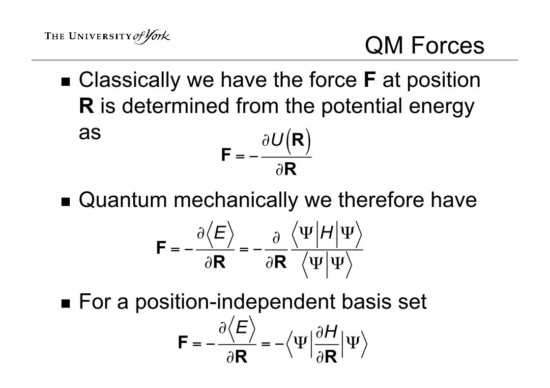
QM Forcesn Classically we have the force F at position R is determined from the potential energy as
n Quantum mechanically we therefore have
n For a position-independent basis set
F = −∂U R( )∂R
F = −∂ E∂R
= −∂∂R
Ψ H Ψ
Ψ Ψ
F = −∂ E∂R
= − Ψ∂H∂R
Ψ
Density Functional Theory (I)
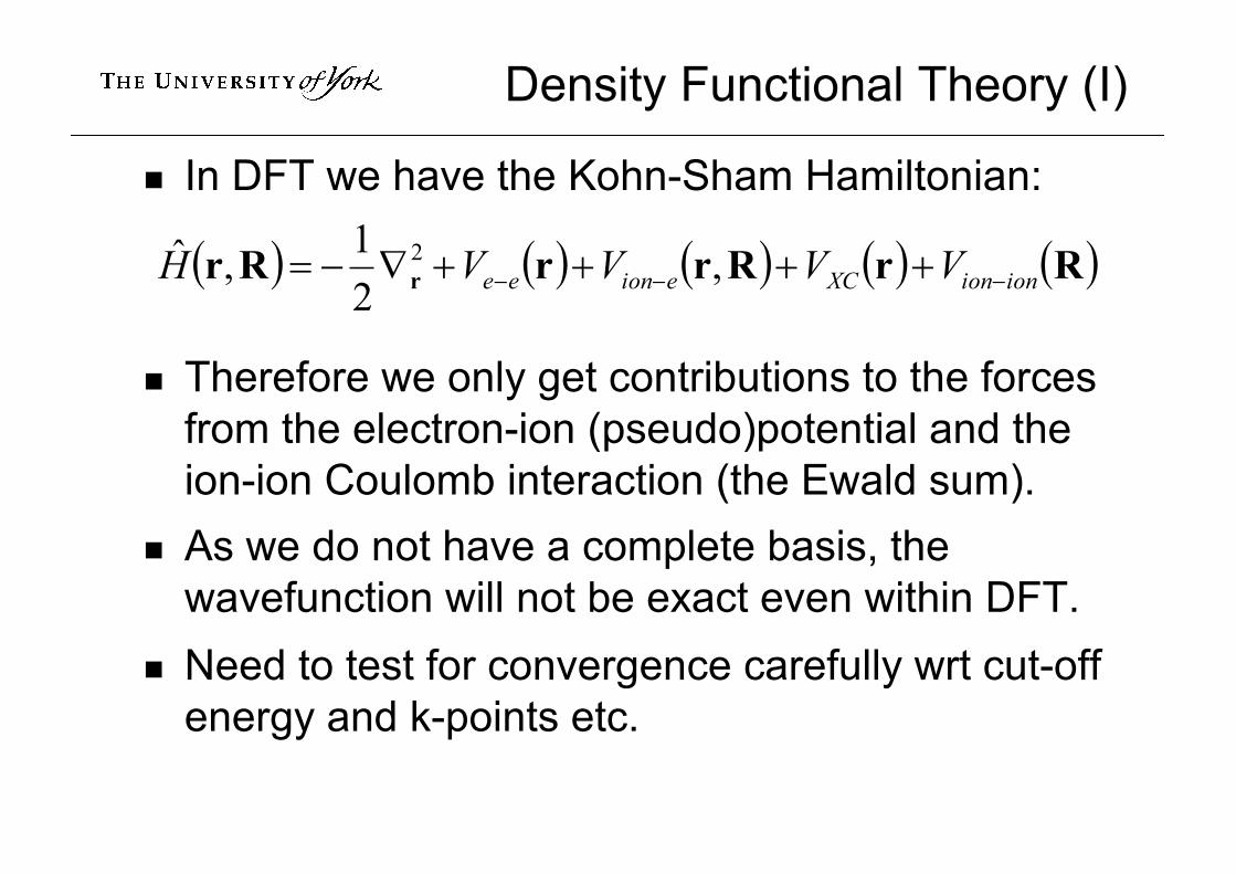
n In DFT we have the Kohn-Sham Hamiltonian:
n Therefore we only get contributions to the forces from the electron-ion (pseudo)potential and the ion-ion Coulomb interaction (the Ewald sum).
n As we do not have a complete basis, the wavefunction will not be exact even within DFT.
n Need to test for convergence carefully wrt cut-off energy and k-points etc.
( ) ( ) ( ) ( ) ( )RrRrrRr r ionionXCeionee VVVVH --- ++++Ñ-= ,21,ˆ 2

Density Functional Theory (II)
n With a variational minimization of the total energy, the energy and wavefunction will be correct to second order errors.n Forces are given by energy differences and
hence get some error cancellationn With a non-variational minimization
technique, such as density mixing, then no upper-bound guaranteed on true E0n So need good convergence if using non-
variational forces and stresses

Quality of Forces/Stresses
n Can only find a good structure if have reliable forces/stresses
n Stresses converge more slowly than energies as increase number of plane wavesn CONVERGENCE!
n Should also check degree of SCF convergenceelec_energy_tol (fine quality ≤ 10-6 eV/atom)
can also set elec_force_tol – useful with DM Stresses converge slower than forces!

How Does Geom Opt Work?n Electrons adjust instantly to position of ions
n Multi-dimensional potential energy surface and want to find global minimum
n Treat as an optimisation problemn Simplest approach is steepest descentsn More physical approach is damped MDn More sophisticated approaches are
conjugate gradients or BFGSn All of these can get stuck in local miniman Hence recent research in how best to find
global minimum
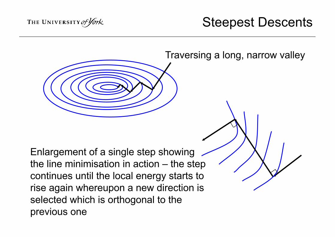
Steepest Descents
Traversing a long, narrow valley
Enlargement of a single step showing the line minimisation in action – the step continues until the local energy starts to rise again whereupon a new direction is selected which is orthogonal to the previous one

Damped MD
Over-dampedUnder-damped
Critically damped
x
t
• Move ions using velocities and forces• Need to add damping term ‘-gv’ to forces• Algorithm to set ‘optimal damping’ factor• Can also adjust dt for max. convergence• More efficient than Steepest Descents
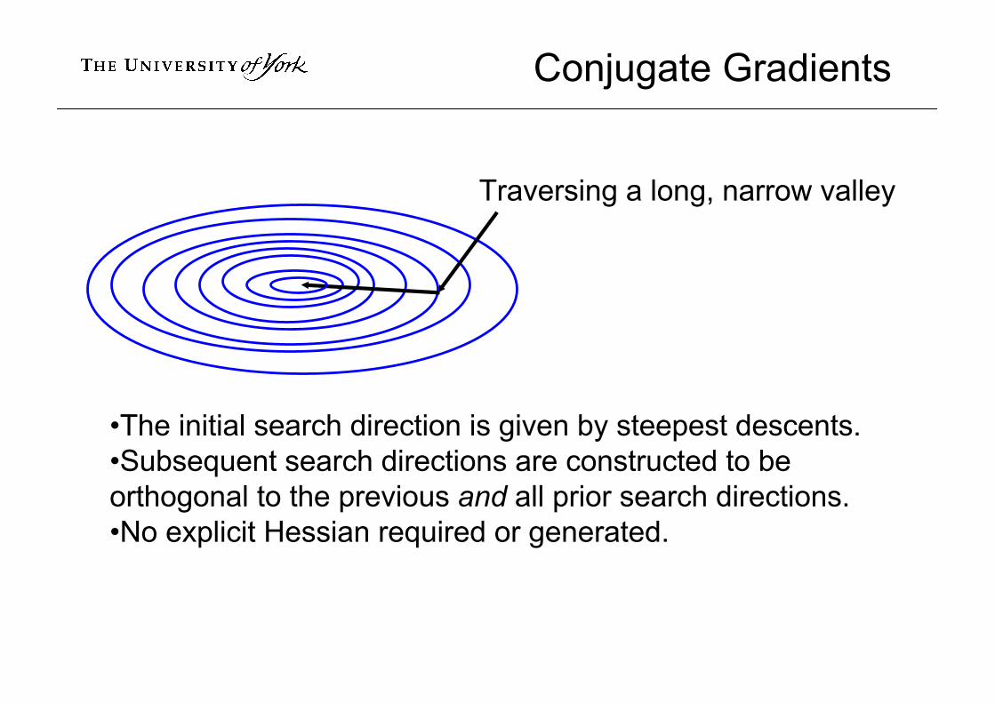
Conjugate Gradients
•The initial search direction is given by steepest descents.•Subsequent search directions are constructed to be orthogonal to the previous and all prior search directions.•No explicit Hessian required or generated.
Traversing a long, narrow valley

BFGS (I)n Basic idea:
n Energy surface around a minima is quadratic in small displacements and so is totally determined by the Hessian matrix A (the matrix of second derivatives of the energy):
n so if we knew A then could move from any nearby point to the minimum in 1 step!
( ) ( )minmin
2
1
2
1
2
11
2
21 XXAXX
A
-••-=
÷÷÷÷
ø
ö
çççç
è
æ
¶¶¶
¶¶¶
¶¶¶
¶¶¶
=
T
NNN
N
E
xxE
xxE
xxE
xxE
d
!

BFGS (II)
n The Problemn We do not know A a priorin Therefore we build up a progressively
improving approximation to A (or the inverse Hessian H=A-1) as we move the ions according to the BFGS (Broyden-Fletcher-Goldfarb-Shanno) algorithm.
n Also known as a quasi-Newton method.n Positions updated according to:
iii
iii
FHXXXX
=DD+=+ l1
CASTEP details

How to do it …
n Just puttask = Geometry Optimisation
in your .param filen Is that all?n What is going on behind the scenes?n What might go wrong?n What can you control?

Choice of Scheme
n geom_method = LBFGS (default)n variable ions and/or celln uses fractional ionic coordinates and strains as
basic variablesn improved estimates based analysis of approx. H built up over convergence path printed at end
n a “low memory” version of geom_method = BFGS which only stores a limited number of updates and not full Hessian

Choice of Schemen geom_method = TPSD
n Very low memory requirementsn No line search and no history
n Ought to be a lot worse than (L)BFGS but we have a smart preconditioner & so not so bad
n Much better than (L)BFGS with constraintsn Much better if start a long way from the harmonic
regionn Can use geom_tpsd_iterchange to switch to
BFGS after given number of TPSD stepsn Can use geom_tpsd_init_stepsize to
control size of initial step

(L)BFGS in CASTEP
§ Trial step performed (default) if geom_use_linmin=true
§ A quadratic system has optimal l=1§ Exact line minimisation has F.DX=0§ Line step only performed if predicted |ltrial-lline| > geom_linmin_tol
No restriction on the value of l as long as does not cause too large an ionic displacement or change in lattice parameters – big advantage of doing a ‘line step’
iii
iii
FHXXXX
=DD+=+ l1
F.DX
l0 1
start
trial
best

Geometry Convergence
n Will continue for geom_max_iter steps (default=30) unless converged:geom_energy_tol (default=2*105 eV/atom)
for geom_convergence_win steps Changing ions:geom_force_tol (default =0.05 eV/Å)geom_disp_tol (default=0.001 Å)Changing cell:geom_stress_tol (default=0.1 GPa)

Variable cell calculations

Variable cell calculations
n If can calculate internal stress then can use this to adjust the cell parameters
n Convention: Pext+ s = 0 at equilibriumn i.e. P>0 = compression, Pint=1/3 Tr(s)n Look for a state of minimum enthalpy
n H=E+PextVn With BFGS we use an augmented Hessian
n Work in space of “fractional positions and strains” with “fractional forces and stresses”
n Then possible to mix cell & ion terms
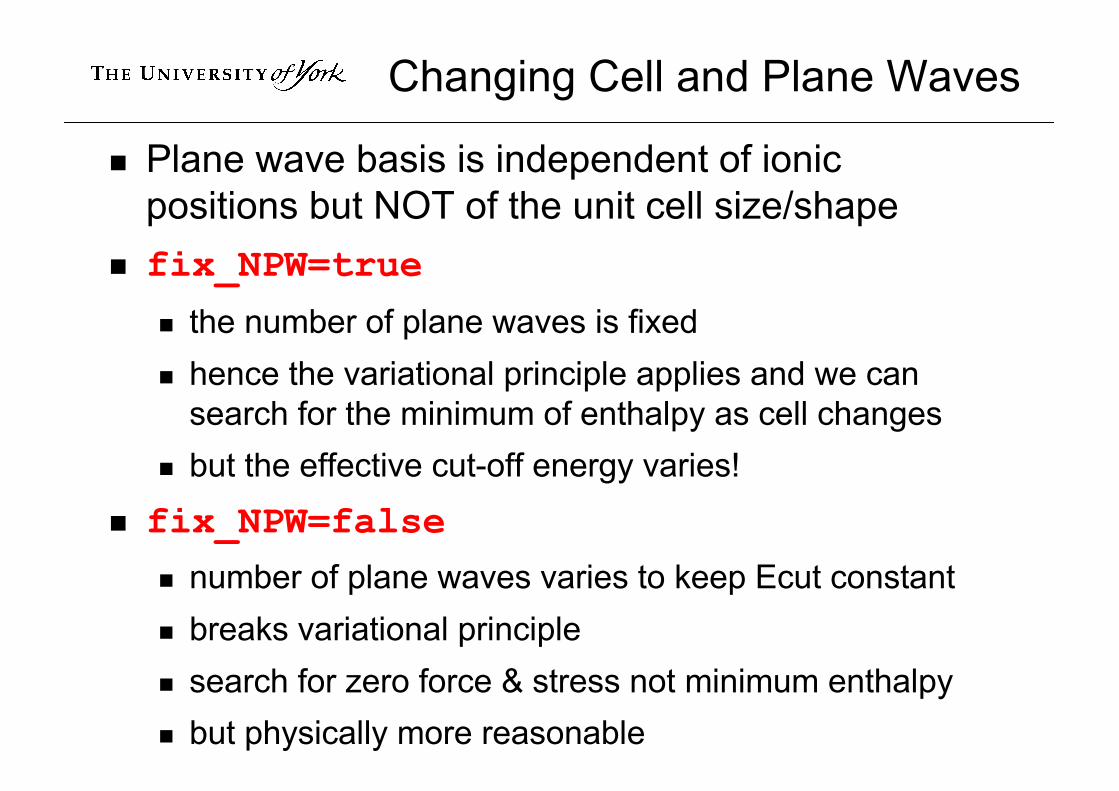
Changing Cell and Plane Waves
n Plane wave basis is independent of ionic positions but NOT of the unit cell size/shape
n fix_NPW=true
n the number of plane waves is fixedn hence the variational principle applies and we can
search for the minimum of enthalpy as cell changesn but the effective cut-off energy varies!
n fix_NPW=falsen number of plane waves varies to keep Ecut constantn breaks variational principlen search for zero force & stress not minimum enthalpyn but physically more reasonable

Finite Basis Set Correction
n Change unit cell at constant cut_off_energy :n changes number of plane-wavesn change in total energy due to variational principlen hence difficult to compare results at different cell sizes.
n Use the Finite Basis Set Correctionn finite_basis_corr = automatic/manual/nonen calculates the total energy finite_basis_npoints
times with finite_basis_spacing change to cut_off_energy at fixed cell
n hence calculates and prints basis_de_dlogen CASTEP can then use this to correct the total energy and
stress at nearby cell sizes


.cell file keywords
fix_all_ions (default = false)fix_all_cell (default = false)fix_com (default = NOT fix_all_ions)symmetry_generatesnap_to_symmetry
%block external_pressure[units]Pxx Pxy Pxz
Pyy PyzPzz
%endblock external_pressureHence hydrostatic P is Pxx=Pyy=Pzz=P and Pxy=Pxz=Pyz=0

Cell Constraints
%block cell_constraints
|a| |b| |c|
a b g%endblock cell_constraints
n Any length (angle) can be held constant (=0), or tied to one or both of the others (=same)n e.g. cell optimisation of 2D structures or
keeping subset of symmetry etcn also fix_vol (= false by default)

Simple Hexagonal cell with symmetry on.
CASTEP constrained-cell optimisation with fix_vol=true
c/a values in good agreement with expt
fix_vol in action

The .geom file
n Records the final configuration after each step:10
-7.93316351E+000 -7.85316331E+000 <-- E
0.00000000E+000 5.13126785E+000 5.13126785E+000 <-- h
5.13126785E+000 0.00000000E+000 5.13126785E+000 <-- h
5.13126785E+000 5.13126785E+000 0.00000000E+000 <-- h
-3.56997760E-003 0.00000000E+000 -3.33783917E-013 <-- S
0.00000000E+000 -3.56997760E-003 8.32597229E-013 <-- S
-3.33783917E-013 8.32597229E-013 5.93008591E-004 <-- S
Si 1 0.00000000E+000 0.00000000E+000 0.00000000E+000 <-- R
Si 2 7.56877069E+000 2.52292356E+000 7.56877069E+000 <-- R
Si 1 -5.22300739E-003 6.43530285E-003 -1.71774942E-003 <-- F
Si 2 5.22300739E-003 -6.43530285E-003 1.71774942E-003 <-- F
n Uses Cartesian coordinates and atomic units throughoutn Designed for other analysis programs, visualisation tools,
etc.

Visualization
n Final geom “trajectory” can be visualized using jmol – just drag & drop .geom file
n Or can add write_cell_structure=true or write_cif_structure=true to output final structure in cell/cif format
n Or can use utilities such as geom2xyz to convert .geom file to .xyz format for visualization by many packages

Ionic Constraints
n Can specify any arbitrary number of linear constraints on the atomic coordinates, up to the number of degrees of freedom. n E.g. fixing an atom, constraining an atom to
move in a line or plane, fixing the relative positions of pairs of atoms, fixing the centre of mass of the system, etc.
n Non-linear constraintsn Much more difficult to apply and specify in
general, e.g. fixing a bond lengthn Only supported by Delocalised Internals
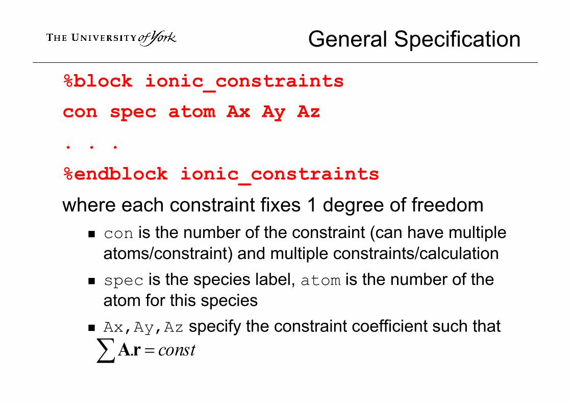
General Specification
%block ionic_constraints
con spec atom Ax Ay Az
. . .
%endblock ionic_constraints
where each constraint fixes 1 degree of freedomn con is the number of the constraint (can have multiple
atoms/constraint) and multiple constraints/calculationn spec is the species label, atom is the number of the
atom for this speciesn Ax,Ay,Az specify the constraint coefficient such thatå = constrA.

Example Linear ConstraintsGeneral format:%block ionic_constraints
1 Si 1 0 0 1
%endblock ionic_constraints
fixes the z-coordinate of the 1st Si atom
Shortcut for fixing 1 or more atoms:%block ionic_constraints
fix: Si 1
%endblock ionic_constraints
Can also do things like fix: all unfix: Hto fix all atoms except H etc.

Summary
Summary
n Need accurate forces and stressesn Pre-requisite for many property calculations
n e.g. phonons, NMR, etc.n Can do optimisation of ions and/or cell
n (L)BFGS or TPSD with Cartesian coordsn Can also for fixed cell use
n BFGS with Cartesian or delocalised internal coordinates, or
n damped MD or FIRE with Cartesians
Useful Referencesn SJ Clark, MD Segall, CJ Pickard, PJ Hasnip, MIJ Probert,
K Refson and MC Payne, “First principles methods using CASTEP”, Zeitschrift für Kristallographie 220, 567 (2005)
n BG Pfrommer, M Cote, SG Louie and ML Cohen “Relaxation of crystals with the quasi-Newton method”, J.Comput. Phys. 131, 233 (1997)
n MIJ Probert, “Improved algorithm for geometry optimisation using damped molecular dynamics”, J. Comput. Phys. 191, 130 (2003)
n E Bitzek, P Koskinen, F Gahler, M Moseler and P Gumbsch, “Structural relaxation made simple” Phys. Rev. Lett. 97 17021 (2006)
n J Andzelm, RD King-Smith, and G Fitzgerald, “Geometry optimization of solids using delocalized internal coordinates”, Chem. Phys. Lett. 335 321 (2001)