Geometry and the Quantum

Alain Connes

March 8, 2017

Contents

1 Introduction 21.1 The spectral point of view . . . . . . . . . . . . . . . . . . . . . . . . . . . . . . . . 21.2 Gravity coupled with matter . . . . . . . . . . . . . . . . . . . . . . . . . . . . . . . 31.3 Possible relevance for Quantum Gravity . . . . . . . . . . . . . . . . . . . . . . . . . 3

2 Prelude: the discrete and the continuum 42.1 Grothendieck’s solution: Topos . . . . . . . . . . . . . . . . . . . . . . . . . . . . . 52.2 Riemann . . . . . . . . . . . . . . . . . . . . . . . . . . . . . . . . . . . . . . . . . . 52.3 The quantum and variability . . . . . . . . . . . . . . . . . . . . . . . . . . . . . . . 8

3 The spectral paradigm 113.1 Why Spectral . . . . . . . . . . . . . . . . . . . . . . . . . . . . . . . . . . . . . . . 123.2 The line element . . . . . . . . . . . . . . . . . . . . . . . . . . . . . . . . . . . . . 143.3 The bonus from non-commutativity . . . . . . . . . . . . . . . . . . . . . . . . . . . 153.4 The notion of manifold . . . . . . . . . . . . . . . . . . . . . . . . . . . . . . . . . . 173.5 Real structure . . . . . . . . . . . . . . . . . . . . . . . . . . . . . . . . . . . . . . . 183.6 The inner fluctuations of the metric . . . . . . . . . . . . . . . . . . . . . . . . . . . 20

4 Quanta of Geometry 224.1 The K-theory higher Heisenberg equation; Spheres . . . . . . . . . . . . . . . . . . 23

4.1.1 One-sided higher Heisenberg equation . . . . . . . . . . . . . . . . . . . . . . 234.1.2 Quantization of volume . . . . . . . . . . . . . . . . . . . . . . . . . . . . . . 234.1.3 Disjoint Quanta . . . . . . . . . . . . . . . . . . . . . . . . . . . . . . . . . . 26

4.2 The KO-theory higher Heisenberg equation . . . . . . . . . . . . . . . . . . . . . . 284.3 Emerging Geometry . . . . . . . . . . . . . . . . . . . . . . . . . . . . . . . . . . . 31

4.3.1 Dimension . . . . . . . . . . . . . . . . . . . . . . . . . . . . . . . . . . . . . 314.3.2 Quantization of volume . . . . . . . . . . . . . . . . . . . . . . . . . . . . . . 32

4.4 Final remarks . . . . . . . . . . . . . . . . . . . . . . . . . . . . . . . . . . . . . . . 32

5 Appendix 33

1

arX

iv:1

703.

0247

0v1

[he

p-th

] 7

Mar

201

7

1 Introduction

The ideas of noncommutative geometry are deeply rooted in both physics, with the predominantinfluence of the discovery of Quantum Mechanics, and in mathematics where it emerged fromthe great variety of examples of “noncommutative spaces” i.e. of geometric spaces which are bestencoded algebraically by a noncommutative algebra.

It is an honor to present an overview of the state of the art of the interplay of noncommutativegeometry with physics on the occasion of the celebration of the centenary of Hilbert’s work on thefoundations of physics. Indeed, the ideas which I will explain, those of noncommutative geometry(NCG) in relation to our model of space-time, owe a lot to Hilbert and this is so in two respects.First of course by the fundamental role of Hilbert space in the formalism of Quantum Mechanics asformalized by von Neumann, see §1.1. But also because, as explained in details in [32, 38], one canconsider Hilbert to be the first person to have speculated about a unified theory of electromagnetismand gravitation, we come to this point soon in §1.2.

1.1 The spectral point of view

At the beginning of the eighties, motivated by the exploration of the many new spaces whose alge-braic incarnation is noncommutative, I introduced a new paradigm, of spectral nature, for geometricspaces. It is based on the Hilbert space formalism of Quantum Mechanics and on mathematicalideas coming from K-theory and index theory. A geometry is given by a “spectral triple” (A,H, D)which consists of an involutive algebra A concretely represented as an algebra of operators in aHilbert space H and of a (generally unbounded) self-adjoint operator D acting on the same Hilbertspace H. The main conceptual motivation came from the work of Atiyah and Singer on the indextheorem and their realization that the Hilbert space formalism was the proper setting for “abstractelliptic operators” [1].

To fix ideas: a compact spin Riemannian manifold is encoded as a spectral triple by letting thealgebra of functions act in the Hilbert space of spinors while the Dirac operator D plays the role ofthe inverse line element, as we shall amply explain below. But the key examples that showed, veryearly on, that the relevance of this new paradigm went far beyond the framework of Riemanniangeometry comprised duals of discrete groups, leaf spaces of foliations and deformations of ordinaryspaces such as the noncommutative tori which were themselves a prime example of noncommutativegeometric spaces as shown in [29].

In the middle of the eighties it became clear that the new paradigm of geometry, because of itsflexibility, provided a new perspective on the geometric interpretation of the detailed structure ofthe Standard model and of the Brout-Englert-Higgs mechanism. Over the years this new pointof view has been considerably refined and is now able to account for the extremely complicatedLagrangian of Einstein gravity coupled to the standard model of particle physics. It is obtainedfrom the spectral action developed in our joint work with A. Chamseddine in [13]. The spectralaction is the only natural additive spectral invariant of a noncommutative geometry.

The noncommutative geometry dictated by physics is the product of the ordinary 4-dimensionalcontinuum by a finite noncommutative geometry which appears naturally from the classificationof finite geometries of KO-dimension equal to 6 modulo 8 (cf. [16, 19]). The compatibility ofthe model with the measured value of the Higgs mass was demonstrated in [21] due to the rolein the renormalization of the scalar field already present in [20]. In [22, 23], with Chamseddine

2

and Mukhanov, we gave the conceptual explanation of the finite noncommutative geometry fromClifford algebras and obtained a higher form of the Heisenberg commutation relations between pand q, whose irreducible Hilbert space representations correspond to 4-dimensional spin geometries.The role of p is played by the Dirac operator and the role of q by the Feynman slash of coordinatesusing Clifford algebras. The proof that all spin geometries are obtained relies on deep results ofimmersion theory and ramified coverings of the sphere. The volume of the 4-dimensional geometryis automatically quantized by the index theorem; and the spectral model, taking into account theinner automorphisms due to the noncommutative nature of the Clifford algebras, gives Einsteingravity coupled with a slight extension of the standard model, which is a Pati-Salam model. Thismodel was shown in our joint work with A. Chamseddine and W. van Suijlekom [25, 26] to yieldunification of coupling constants.

1.2 Gravity coupled with matter

As explained in detail in [32], one can consider Hilbert as the first to have fancied a unified theory ofelectromagnetism and gravitation. According to [32], in the course of pursuing this agenda, Hilbertreversed his original idea of founding all of physics on electrodynamics, instead treating the gravi-tational field equations as more fundamental. We have, in our investigations with Ali Chamseddineof the fine structure of space-time which is revealed by the Brout-Englert-Higgs mechanism, fol-lowed a parallel path: the starting point was that the NCG framework for geometry, by allowingto treat the discrete and the continuum on the same footing gives a clear geometric meaning to theBrout-Englert-Higgs sector of the Standard Model, as the signal of a discrete (but finite) componentof the geometry of space-time appearing as a fine structure which refines the usual 4-dimensionalcontinuum.

The action principle however was at the beginning of the theory still of traditional form (see [28]).In our joint work with Ali Chamseddine [13] we understood that instead of imitating the traditionalform of the Yang-Mills action, one could obtain the full package of the Einstein-Hilbert action1

of gravity coupled with matter by a fundamental spectral principle. In the language of NCG thisprinciple asserts that the action only depends upon the “line element” i.e. the inverse2 of the operatorD. It follows then from elementary considerations of additivity for disjoint unions of spaces thatit must be of the form Tr(f(D/Λ)) where f is a function and Λ is a parameter having the samedimension (that of an energy) as the inverse line element D.

1.3 Possible relevance for Quantum Gravity

It will by now be clear to the reader that the point of view adopted in this essay is to try tounderstand from a mathematical perspective, how the perplexing combination of the Einstein-Hilbert action coupled with matter, with all the subtleties such as the Brout-Englert-Higgs sector,the V-A and the see-saw mechanisms etc.. can emerge from a simple geometric model. The newtool is the spectral paradigm and the new outcome is that geometry does emerge on the stage whereQuantum Mechanics happens, i.e. Hilbert space and linear operators.

1There is a well-known “priority episode” between Hilbert and Einstein which is discussed in great detail in [32,38]and whose outcome, called the Einstein-Hilbert action, plays a key role in our approach

2In the orthogonal complement of its kernel

3

The idea that group representations as operators in Hilbert space are relevant to physics is ofcourse very familiar to every particle theorist since the work of Wigner and Bargmann. That theformalism of operators in Hilbert space encompasses the variable geometries which underly gravityis the leitmotiv of our approach.

In order to estimate the potential relevance of this approach to Quantum Gravity, one first needsto understand the physics underlying the problem of Quantum Gravity. There is an excellentarticle for this purpose: the paper [47] explains how the problem arises when one tries to apply theperturbative method (which is so successful in quantum field theory) to the Lagrangian of gravitycoupled with matter. Quoting from [47]: “Quantization of gravity is inevitable because part of themetric depends upon the other fields whose quantum nature has been well established”.

Two main points are that the presence of the other fields forces one, due to renormalization, to addhigher derivative terms of the metric to the Lagrangian and this in turns introduces at the quantumlevel an inherent instability that would make the universe blow up. This instability is instantlyfatal to an interacting quantum field theory. Moreover primordial inflation prevents one from fixingthe problem by discretizing space at a very small length scale. What our approach permits isto develop a “particle picture” for geometry; and a careful reading of the present paper shouldhopefully convince the reader that this particle picture stays very close to the inner workings of theStandard Model coupled to gravity. For now the picture is limited to the “one-particle” descriptionand there are deep purely mathematical reasons to develop the many particles picture. The mainone is that the root of the one-particle picture, described by spectral triples, is KO-homology andthe dual topological KO-theory (see §3.4). The duality between the two theories is the originof the quanta of geometry given by irreducible representations of the higher Heisenberg relationdescribed in §4 below. As already mentioned in [27], algebraic K-theory, which is a vast refinementof the topological theory, is begging for the development of a dual theory and one should expectprofound relations between this dual theory and the theory of interacting quanta of geometry. As aconcrete point of departure, note that the deepest results on the topology of diffeomorphism groupsof manifolds are given by the Waldhausen algebraic K-theory of spaces and we refer to [33] for aunifying picture of algebraic K-theory. For this paper, we now we discuss in depth the problem ofthe co-existence of the discrete and the continuum in geometry.

Acknowledgement. I am grateful to Joseph Kouneiher and Jeremy Butterfield for their help inthe elaboration of this paper.

2 Prelude: the discrete and the continuum

In this preliminary section we shall discuss two solutions of the mathematical problem of treatingthe continuous and the discrete in a unified manner. We first briefly present Grothendieck’s solution:the notion of a topos which allowed him to treat in a unified manner ordinary topological spacesand the combinatorial structures arising in the world of arithmetic. We continue with a text ofGrothendieck on Riemann as a prelude for a re-reading of Riemann’s inaugural lecture. We thenexplain how the quantum formalism provides another solution to the coexistence of discrete andcontinuous variables.

4

2.1 Grothendieck’s solution: Topos

Grothendieck’s solution to the problem of treating the continuous and the discrete in a unifiedmanner is the notion of a Topos. It does reconcile the usual idea of a topological space with that ofa discrete combinatorial diagram. One does not concentrate on the space X itself, with its pointsetc... but rather on the ability of X to define a variable set Zx depending on x ∈ X. When X isan ordinary topological space such a “variable set” indexed by X is simply a sheaf of sets on X.But this continues to make sense starting from an abstract combinatorial diagram! In short the keyidea here is the idea of replacing X by its role as a parameter space

“Space X → Category of variable sets with parameter in X”

The abstract categories of such “sets depending on parameters” fulfill almost all properties ofthe category of sets, except the axiom of the excluded middle, and encode in a faithful manner atopological space X through the category of sheaves of sets on X. This new idea is amazing in itssimplicity, its connection with logics and the richness of the new class of spaces that it uncovers. InGrothendieck’s own words (see “Recoltes et Semailles” [35,39]) one can sense his amazement :

“Le “principe nouveau” qui restait a trouver, pour consommer les epousailles promisespar des fees propices, ce n’etait autre aussi que ce “lit” spacieux qui manquait aux futursepoux, sans que personne jusque-la s’en soit seulement apercu. . .

Ce “lit a deux places” est apparu (comme par un coup de baguette magique. . .) avecl’idee du topos. Cette idee englobe, dans une intuition topologique commune, aussi bienles traditionnels espaces (topologiques), incarnant le monde de la grandeur continue, queles (soi-disant) “espaces” (ou “varietes”) des geometres algebristes abstraits impenitents,ainsi que d’innombrables autres types de structures, qui jusque-la avaient semble riveesirremediablement au “monde arithmetique” des agregats “discontinus” ou “discrets”.

I would like to stress a key point of Grothendieck’s idea of topos by using a metaphor. From hispoint of view, one understands a geometric space not by directly staring at it: no, the space remainsat the back of the stage as a hidden schemer which governs the variability of every object at thefront of the stage which is occupied by the usual suspects such as “abelian groups” for instance. Butonce one studies these usual suspects in their new environment one finds that their fine propertiesreveal, from their relations with ordinary abelian groups, the cohomology of the hidden parameterspace. Here the word “ordinary” means “independent of the parameter” and thus ordinary setsform part of the new set theory. This makes sense because a Grothendieck topos admits a uniquemorphism to the topos of sets.

2.2 Riemann

In the prelude of “Recoltes et Semailles” [35], Alexandre Grothendieck makes the following pointson the search for relevant geometric models for physics and on Riemann’s lecture on the foundationsof geometry: (see Appendix §5 for the English translation)

“Il doit y avoir deja quinze ou vingt ans, en feuilletant le modeste volume constituantl’œuvre complete de Riemann, j’avais ete frappe par une remarque de lui “en passant”.

5

Il y fait observer qu’il se pourrait bien que la structure ultime de l’espace soit “discrete”,et que les representations “continues” que nous nous en faisons constituent peut-etreune simplification (excessive peut-etre, a la longue. . .) d’une realite plus complexe ; quepour l’esprit humain, “le continu” etait plus aise a saisir que “le discontinu”, et qu’ilnous sert, par suite, comme une “approximation” pour apprehender le discontinu.

C’est la une remarque d’une penetration surprenante dans la bouche d’un mathematicien,a un moment ou le modele euclidien de l’espace physique n’avait jamais encore ete misen cause ; au sens strictement logique, c’est plutot le discontinu qui, traditionnellement,a servi comme mode d’approche technique vers le continu.

Les developpements en mathematique des dernieres decennies ont d’ailleurs montre unesymbiose bien plus intime entre structures continues et discontinues, qu’on ne l’imaginaitencore dans la premiere moitie de ce siecle. Toujours est-il que de trouver un modele“satisfaisant” (ou, au besoin, un ensemble de tels modeles, se “raccordant” de faconaussi satisfaisante que possible. . .), que celui-ci soit “continu”, “discret” ou de nature“mixte” – un tel travail mettra en jeu surement une grande imagination conceptuelle, etun flair consomme pour apprehender et mettre a jour des structures mathematiques detype nouveau.

Ce genre d’imagination ou de “flair” me semble chose rare, non seulement parmi lesphysiciens (ou Einstein et Schrodinger semblent avoir ete parmi les rares exceptions),mais meme parmi les mathematiciens (et la je parle en pleine connaissance de cause).

Pour resumer, je prevois que le renouvellement attendu (s’il doit encore venir. . .) vien-dra plutot d’un mathematicien dans l’ame, bien informe des grands problemes de laphysique, que d’un physicien. Mais surtout, il y faudra un homme ayant “l’ouverturephilosophique” pour saisir le nœud du probleme. Celui-ci n’est nullement de naturetechnique, mais bien un probleme fondamental de “philosophie de la nature”.

After reading the above text of Grothendieck, let us go to the relevant part of Riemann’s Habilita-tion lecture on the foundations of geometry and explain why his great insight is, together with theadvent of quantum mechanics, the best prelude to the new paradigm of spectral triples, the basicgeometric concept in NCG.

“Wenn aber eine solche Unabhangigkeit der Korper vom Ort nicht stattfindet, so kannman aus den Massverhaltnissen im Grossen nicht auf die im Unendlichkleinen schliessen;es kann dann in jedem Punkte das Krummungsmass in drei Richtungen einen beliebi-gen Werth haben, wenn nur die ganze Krummung jedes messbaren Raumtheils nichtmerklich von Null verschieden ist; noch complicirtere Verhaltnisse konnen eintreten,wenn die vorausgesetzte Darstellbarkeit eines Linienelements durch die Quadratwurzelaus einem Differentialausdruck zweiten Grades nicht stattfindet. Nun scheinen aber dieempirischen Begriffe, in welchen die raumlichen Massbestimmungen gegrundet sind, derBegriff des festen Korpers und des Lichtstrahls, im Unendlichkleinen ihre Gultigkeit zuverlieren; es ist also sehr wohl denkbar, dass die Massverhaltnisse des Raumes im Un-endlichkleinen den Voraussetzungen der Geometrie nicht gemass sind, und dies wurdeman in der That annehmen mussen, sobald sich dadurch die Erscheinungen auf ein-fachere Weise erklaren liessen.

6

Die Frage uber die Gultigkeit der Voraussetzungen der Geometrie im Unendlichkleinenhangt zusammen mit der Frage nach dem innern Grunde der Massverhaltnisse desRaumes. Bei dieser Frage, welche wohl noch zur Lehre vom Raume gerechnet wer-den darf, kommt die obige Bemerkung zur Anwendung, dass bei einer discreten Mannig-faltigkeit das Princip der Massverhaltnisse schon in dem Begriffe dieser Mannigfaltigkeitenthalten ist, bei einer stetigen aber anders woher hinzukommen muss. Es muss alsoentweder das dem Raume zu Grunde liegende Wirkliche eine discrete Mannigfaltigkeitbilden, oder der Grund der Massverhaltnisse ausserhalb, in darauf wirkenden bindenenKraften, gesucht werden.

Die Entscheidung dieser Fragen kann nur gefunden werden, indem man von der bish-erigen durch die Erfahrung bewahrten Auffassung der Erscheinungen, wozu Newton denGrund gelegt, ausgeht und diese durch Thatsachen, die sich aus ihr nicht erklaren lassen,getrieben allmahlich umarbeitet; solche Untersuchungen, welche, wie die hier gefuhrte,von allgemeinen Begriffen ausgehen, konnen nur dazu dienen, dass diese Arbeit nichtdurch die Beschranktheit der Begriffe gehindert und der Fortschritt im Erkennen desZusammenhangs der Dinge nicht durch uberlieferte Vorurtheile gehemmt wird.

Es fuhrt dies hinuber in das Gebiet einer andern Wissenschaft, in das Gebiet der Physik,welches wohl die Natur der heutigen Veranlassung nicht zu betreten erlaubt”.

This can be translated as follows:“But if the independence of bodies from position is not fulfilled, we cannot draw conclusions from

metric relations of the large, to those of the infinitely small; in that case the curvature at eachpoint may have an arbitrary value in three directions, provided that the total curvature of everymeasurable portion of space does not differ sensibly from zero. Still more complicated relations mayexist if we no longer assume that the line element is expressible as the square root of a quadraticdifferential. Now it seems that the empirical notions on which the metric determinations of spaceare based, the notion of solid body and of ray of light, cease to be valid for the infinitely small. Weare therefore quite free to assume that the metric relations of space in the infinitely small do notcomply with the hypotheses of geometry; and we ought in fact to do this, if we can thereby obtaina simpler explanation of phenomena.

The question of the validity of the hypotheses of geometry in the infinitely small is tied up withthe question of the origin of the metric relations of space. In this last question, which we may stillregard as belonging to the doctrine of space, is found the application of the remark made above; thatin a discrete manifold, the origin of its metric relations is given intrinsically, while in a continuousmanifold, this origin must come from outside. Either therefore the reality which underlies spacemust form a discrete manifold, or we must seek the origin of its metric relations outside it, in thebinding forces which act upon it.

The answer to these questions can only be obtained by starting from the conception of phenomenawhich has hitherto been justified by experiments, and which Newton assumed as a foundation,and by making in this conception the successive changes required by facts which it cannot explain.Researches starting from general notions, like the investigation we have just made, can only be usefulin preventing this work from being hampered by too narrow views, and progress in knowledge ofthe interdependence of things from being prevented by traditional prejudices.

7

This leads us into the domain of another science, of physics, into which the object of this workdoes not allow us to enter today.”

2.3 The quantum and variability

The originality of the quantum world (in which we actually live) as compared to its classical ap-proximation, is already manifest at the experimental level by the “imaginative randomness” of theresults of experiments in the microscopic world. In order to appreciate this point consider the prob-lem of manufacturing a random number generator in such a way that even if an attacker happensto know the full details of the system the chance of reproducing the outcome is zero. This problemwas solved concretely by Bruno Sanguinetti, Anthony Martin, Hugo Zbinden, and Nicolas Gisinfrom the Group of Applied Physics, University of Geneva (see [34]). They invented : “A genera-tor of random numbers of quantum origin using technology compatible with consumer and portableelectronics and whose simplicity and performance will make the widespread use of quantum randomnumbers a reality, with an important impact on information security.”

Figure 1: The device uses the light emitted by a LED to produce a random number based on thequantum randomness of which cells of the camera are reached by emitted photons. This figure istaken from [34].

This inherent randomness of the quantum world is not totally arbitrary since when the observablequantities that one measures happen to commute the usual classical intuition does apply. We owe toWerner Heisenberg the discovery3 that the order of terms does matter when one deals with physicalquantities which pertain to microscopic systems. We shall come back later in §3.3 to the meaning ofthis fact but for now we retain that when manipulating the observables quantities for a microscopicsystem, the order of terms in a product plays a crucial role.

3which he did while he was in the Island of Helgoland trying to recover from hay fever away from pollen sources

8

Figure 2: Birdseye view, Helgoland, Germany, between 1890 and 1900. Image available from theUnited States Library of Congress’s Prints and Photographs division, digital ID ppmsca.00573.

The commutativity of Cartesian coordinates does not hold in the algebra of coordinates on thephase space of a microscopic system. What Heisenberg discovered was that quantum observablesobey the rules of matrix mechanics and this led von Neumann to formalize quantum mechanics interms of operators on Hilbert space. Let us explain now why this formalism actually provides amathematical notion of “real variable” which allows for the coexistence of continuous and discretevariables. Let us first display the defect of the classical notion. In the classical formulation of realvariables as maps from a set X to the real numbers R, the set X has to be uncountable if somevariable has continuous range. But then for any other variable with countable range some of themultiplicities are infinite. This means that discrete and continuous variables cannot coexist in thisclassical formalism.

Fortunately everything is fine and this problem of treating continuous and discrete variables onthe same footing is completely solved using the formalism of quantum mechanics which providesanother solution and treats directly the notion of real variable. The key replacement is

“Real Variable → Self Adjoint Operator in Hilbert space”

All the usual attributes of real variables such as their range, the number of times a real numberis reached as a value of the variable etc... have a perfect analogue in the quantum mechanicalsetting. The range is the spectrum of the operator, and the spectral multiplicity gives the numberof times a real number is reached. It is very comforting for instance that one can compose anymeasurable (Borel) map h : R→ R with any self-adjoint operator H so that h(H) makes sense andhas the expected property of the composed real variable. In the early times of quantum mechanics,physicists had a clear intuition of this analogy between operators in Hilbert space (which they calledq-numbers) and variables. Note that the choice of Hilbert space is irrelevant here since all separableinfinite dimensional Hilbert spaces are isomorphic.

9

Classical Quantum

Real variable Self-adjointf : X → R operator in Hilbert space

Possible values Spectrum ofof the variable the operator

Algebraic operations Algebra of operatorson functions in Hilbert space

In fact it is the uniqueness of the separable infinite dimensional Hilbert space that cures theabove problem of coexistence of discrete and continuous variables: L2[0, 1] is the same as `2(N),and variables with continuous range (such as the operator of multiplication by x ∈ [0, 1]) coexisthappily with variables with countable range (such as the operator of multiplication by 1/n, n ∈ N),but they do not commute!

It is only because one drops commutativity that variables with continuous range can coexist withvariables with countable range. The only new fact is that they do not commute, and the realsubtlety is in their algebraic relations.

What is surprising is that the new set-up immediately provides a natural home for the “infinitesimalvariables”: and here the distinction between “variables” and numbers (in many ways this is wherethe point of view of Newton is more efficient than that of Leibniz) is essential. It is worth quotingNewton’s definition of variables and of infinitesimals, as opposed to Leibniz:

“In a certain problem, a variable is the quantity that takes an infinite number of valueswhich are quite determined by this problem and are arranged in a definite order”

“A variable is called infinitesimal if among its particular values one can be found suchthat this value itself and all following it are smaller in absolute value than an arbitrarygiven number”

Indeed it is perfectly possible for an operator to be “smaller than epsilon for any epsilon” withoutbeing zero. This happens when the norm of the restriction of the operator to subspaces of finitecodimension tends to zero when these subspaces decrease (under the natural filtration by inclusion).The corresponding operators are called “compact” and they share with naive infinitesimals all theexpected algebraic properties.

10

Classical Quantum

Infinitesimal Compactvariable operator in Hilbert space

Infinitesimal of µn(T ) of size n−α

order α when n→∞

Integral of

∫−T = coefficient of

function∫f(x)dx log(Λ) in TrΛ(T)

Indeed they form a two-sided ideal of the algebra of bounded operators in Hilbert space and theonly property of the naive infinitesimal calculus that needs to be dropped is the commutativity.

The calculus of infinitesimals fits perfectly into the operator formalism of quantum mechanicswhere compact operators play the role of infinitesimals, with order governed by the rate of decay ofthe characteristic values, and where the logarithmic divergences familiar in physics give the substi-tute for integration of infinitesimals of order one, in the form of the Dixmier trace and Wodzicki’s

residue. We refer to [28] for a detailed description of the new integral

∫−.

3 The spectral paradigm

Before we start the “inward bound” trip [42] to very small distances, it is worth explaining how thespectral point of view helps also when dealing with issues connected to large astronomical distances.

The simple question “Where are we?” does not have such a simple answer since giving our coor-dinates in a specific chart is not an invariant manner of describing our position. We refer to Figure3 for one attempt at an approximate answer.

In fact it is not obvious how to solve two mathematical questions which naturally arise in thiscontext:

1. Can one specify a geometric space in an invariant manner?

2. Can one specify a point of a geometric space in an invariant manner?

11

Figure 3: The pioneer 4 probe, picture from NASA : 668774 main pioneer plaque.

3.1 Why Spectral

Given a compact Riemannian space one obtains a slew of geometric invariants of the space byconsidering the spectrum of natural operators such as the Laplacian. The obtained list of numbersis a bit like a scale associated to the space as made clear by Mark Kac in his famous paper4 “Can onehear the shape of a drum?”. It is well known however since a famous one page paper5 of John Milnorthat the spectrum of operators, such as the Laplacian, does not suffice to characterize a compactRiemannian space. But it turns out that the missing information is encoded by the relative positionof two abelian algebras of operators in Hilbert space. Due to a theorem of von Neumann, the algebraof multiplication by all measurable bounded functions acts in Hilbert space in a unique manner,independent of the geometry one starts with. Its relative position with respect to the other abelianalgebra given by all functions of the Laplacian suffices to recover the full geometry, provided oneknows the spectrum of the Laplacian. For some reason which has to do with the inverse problem,it is better to work with the Dirac operator; and as we shall explain now, this gives a guess for anew incarnation of the “line element”. The Riemannian paradigm is based on the Taylor expansionin local coordinates of the square of the line element, and in order to measure the distance betweentwo points one minimizes the length of a path joining the two points as in Figure 4

d(a, b) = Inf

∫γ

√gµ ν dxµ dxν (1)

4Kac, Mark (1966), ”Can one hear the shape of a drum?”, American Mathematical Monthly 73 (4, part 2): 1–235Milnor, John (1964), ”Eigenvalues of the Laplace operator on certain manifolds”, Proceedings of the National

Academy of Sciences of the United States of America 51

12

Figure 4: Geodesic Figure 5: Delambre and Mechain

Great efforts were done at the time of the French revolution in order to obtain a sensible unificationof the various units of length that were in use across the country. It was decided (by Louis XVI,under the advice of Lavoisier) to take, as a unit, the length L such that 4 × 106L would be thecircumference of the earth. After using as a preliminary reduction the computation of angles fromastronomical observations to reduce the actual measurement to a smaller portion of meridian, ateam was sent out in 1792 to make the precise measurement of the distance between Dunkerquein the north of France and Barcelona in Spain; see Figure 5. This measurement6 resulted in anincarnation of L as a concrete platinum bar that was kept in Pavillon de Breuteuil near Paris. Iremember learning in school this definition of the “meter”.

However it turned out that in the 1930’s, physicists were able to decide that the above choice ofL was no good. Not only because it would seem totally unpractical if we would for instance try totransmit its definition to a far distant star, but for a more pragmatic reason, they observed that theconcrete platinum bar defining L actually had a non-constant length! This observation was doneby comparing it with a specific wave length of Krypton.

Figure 6: Meter → Wave length, the 13th CGPM (1967) uses hyperfine levels of Cesium (C133).Adaptation of original found at hyperphysics.phy-astr.gsu.edu

6I refer the reader to [3] for a very interesting and more detailed account of the story of the measurement performedby Delambre and Mechain

13

Then it took some time until they decided to take the obvious step: to replace L by the wavelengthof a specific atomic transition (the chosen one is called 2S1/2 of Cesium 133), as was done in 1967.

More precisely, this hyperfine transition is used to define the second as the duration of 9 192 631770 periods of the radiation corresponding to the transition between the two hyperfine levels of theground state of the cesium 133 atom.

Moreover the speed of light is set to the value of 299792458 meters/second, which thus defines themeter as the length of the path travelled by light in vacuum during a time interval of 1/299 792458 of a second, i.e. the meter is

9192631770

299792458=

656616555

21413747∼ 30.6633

times the wavelength of the hyperfine transition of Cesium (which is of the order of 3.26cm).What is manifest with this new choice of L is that one now has a chance to be able to communicate

our “unit of length” with aliens without telling them to come to Paris etc... Probably in fact thisissue should motivate us to choose a chemical element such as hydrogen which is far more commonin the universe than Cesium. One striking advantage of the new choice of L is that it is no longer“localized” (as it was before near Paris) and is available anywhere using the constancy of the spectralproperties of atoms. It will serve us as a motivation for our spectral paradigm.

3.2 The line element

The presence of the square root in (1) is the witness of Riemann’s prescription for the square of theline element as ds2 = gµ ν dx

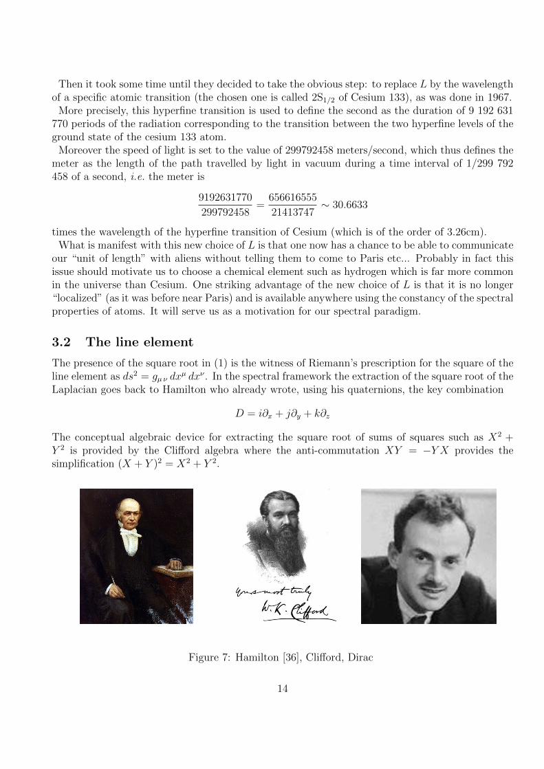
µ dxν . In the spectral framework the extraction of the square root of theLaplacian goes back to Hamilton who already wrote, using his quaternions, the key combination

D = i∂x + j∂y + k∂z

The conceptual algebraic device for extracting the square root of sums of squares such as X2 +Y 2 is provided by the Clifford algebra where the anti-commutation XY = −Y X provides thesimplification (X + Y )2 = X2 + Y 2.

Figure 7: Hamilton [36], Clifford, Dirac

14

P. Dirac showed how to extract the square root of the Laplacian in order to obtain a relativisticform of the Schrodinger equation. For curved spaces Atiyah and Singer devised a general formulafor the Dirac operator on a spin Riemannian manifold and this provides us with our prescription:the line element is the propagator

ds = D−1

(where one takes the value 0 on the kernel). This allows us to measure distances and (1) becomes

d(a, b) = Sup |f(a)− f(b)|, f such that ‖[D, f ]‖ ≤ 1. (2)

which gives the same answer as (1) and is a “Kantorovich dual” of the usual formula. But we nowhave the possibility to define and measure distances without the need of paths joining two pointsas in (1). And indeed one finds plenty of examples of totally disconnected spaces in which thenew formula (2) makes sense and gives sensible results while (1) would not, due to the absence ofconnected arcs.

Figure 8: Line Element

The link of this new definition of distances (and hence of geometry) with the quantum worldappears in many ways: first the “line element” ought to be an “infinitesimal”. This indeed fitssince in a compact Riemannian spin manifold the above operator ds is compact i.e. infinitesimalas explained in §2.3. But there are two more facts which help us to appreciate the relevance ofthe new concept: both are displayed in Figure 8. In the upper part the directed line is a commoningredient of Feynman diagrams, it represents the internal legs of fermionic diagrams and is calledthe “fermion propagator”. Physically it represents a very tiny interval in which the interactiontakes place. Mathematically it is our “ds” (modulo a bit of agility in understanding the physicslanguage and in particular the need to pass from the Minkowski signature to the Euclidean one).The lower part of Figure 8 displays an even more important feature: the above fermionic propagatorundergoes quantum corrections due to its role in quantum field theory and we can interpret thesecorrections as quantum corrections to the geometry!

3.3 The bonus from non-commutativity

In algebra the commutativity assumption often appears as a welcome simplification which makesmany algebraic manipulations much easier. But in fact we should realize that our use of the writtenlanguage makes us perfectly familiar with non-commutativity. The advantage, as far as meaningis concerned, of paying attention to the order of terms, becomes clear when considering anagrams

15

i.e. writings which become equal when “abelianized” but nevertheless have quite different meaningswhen the order of terms is respected. Here is a recent anagram which can be found in “Anagrammespour lire dans les pensees” by Raphael Enthoven and Jacques Perry-Salkow,

“ondes gravitationnelles”

“le vent d’orages lointains”

When we permit ourselves to commute the various letters involved in each of these phrases wefind the same result:

a2de3gi2l2n3o2rs2t2v

This shows that in projecting a phrase in the commutative world one looses an enormous amountof information encoded by non-commutativity. Natural languages respect non-commutativity anda phrase is a much more informative datum than its commutative algebraic shadow.

Here are two more key features of the noncommutative world:

1. Non-commuting discrete variables of the simplest kind generate continuous variables.

2. A noncommutative algebra possesses inner automorphisms.

We always think of variables through their representations as operators in Hilbert space as explainedin §2.3 and since the product of two self-adjoint operators is not self-adjoint unless they commute,one deals with algebras A which are ∗-algebras i.e. which are endowed with an antilinear involutionwhich obeys the rule (xy)∗ = y∗x∗ for any x, y ∈ A. The simplest noncommutative algebra of thiskind is M2(C) the algebra of 2× 2 matrices

a =

(a11 a12

a21 a22

), b =

(b11 b12

b21 b22

), ab =

(a11b11 + a12b21 a11b12 + a12b22

a21b11 + a22b21 a21b12 + a22b22

)and the antilinear involution is given using the complex conjugation z 7→ z by the conjugatetranspose, i.e.

a∗ =

(a11 a21

a12 a22

)This algebra M2(C) only represents discrete variables taking at most two values but as soon as oneadjoins another non-commuting variable Y , such that Y = Y ∗ and Y 2 = 1 one generates all matrixvalued functions on the two-sphere.

To be more precise, write the above generic matrix in the form a = a11e11 +a12e12 +a21e21 +a22e22

where the eij ∈ M2(C), and the coefficients aij ∈ C are complex numbers. Then using algebra onecan write Y = y11e11 + y12e12 + y21e21 + y22e22 where the yij are no longer complex numbers butcommute with M2(C). For instance y11 = e11Y e11 + e21Y e12. One imposes the additional conditionthat the trace of Y is zero, i.e. that y11 + y22 = 0. It is then an exercise using the relations Y = Y ∗

and Y 2 = 1, to show that the C∗-algebra generated by the yij is the algebra C(S2) of continuousfunctions on the two sphere S2. It contains of course plenty of “continuous variables” and thetraditional sup norm of complex valued functions is

Supx∈S2|f(x)| = Supπ‖π(f)‖

16

where in the right hand side π runs through all Hilbert space representations (compatible with theinvolution ∗) of the above relations. One obtains all continuous functions by completion and thusone keeps inside the algebra C(S2) the nicer smooth functions such as those algebraically obtainedfrom the yij. The sphere itself is recovered as the Spectrum of the algebra, and the points of thesphere are the characters i.e. the morphisms of involutive algebras to C.

This is a prototype example of how a connected space (here the two sphere S2) can spring out ofthe discrete (here M2(C) and the two valued variable Y ) due to non-commutativity. Note also thecompatibility of the two notions of spectrum. Indeed for f in the commutative algebra generatedby the yij, the spectrum of the operator π(f) is the image by the corresponding function on S2 ofthe support of the representation π which is a closed subset of the spectrum of the algebra. To putthis in a suggestive manner: what happens is that the geometric space S2 appeared in a spectralmanner and from familiar players of the quantum world: the algebra M2(C), for instance, is familiarfrom spin systems.

There is another great bonus from non-commutativity: the natural algebra which springs out ofthe non-commuting M2(C) and Y discussed above is not the algebra generated by the yij but thealgebra generated by M2(C) and Y . It contains the former but is larger and gives the algebraC(S2,M2(C)) of matrix valued continuous functions on the two sphere. If we take the subalgebraof smooth functions A = C∞(S2,M2(C)) (which is canonically obtained inside C(S2,M2(C)) byapplying the smooth functional calculus to the generators) and one looks at its automorphismgroup7, one finds that it fits in an exact sequence

1→ Int(A)→ Aut(A)→ Out(A)→ 1.

Such an exact sequence exists for any non-commutative ∗-algebra, the inner automorphisms Int(A)are those of the form x 7→ uxu∗ where u ∈ A is a unitary element i.e. fulfills uu∗ = u∗u = 1. Thenice general fact is that these automorphisms always form a normal subgroup of the group Aut(A)and the quotient group Out(A) is called the group of outer automorphisms of A. Now when onecomputes these groups in our example i.e. for A = C∞(S2,M2(C)), one finds that the group Out(A)is the group of diffeomorphisms Diff(S2) while Int(A) is the group of smooth maps from S2 to theLie group PSU(2) whose Lie algebra is su(2). Thus we witness in this example the marriage of thegauge group of gravity i.e. the diffeomorphism group, with the gauge group of matter i.e. here ofan su(2)-gauge theory.

3.4 The notion of manifold

The notion of spectral geometry has deep roots in pure mathematics. They have to do with theunderstanding of the notion of (smooth) manifold. While this notion is simple to define in termsof local charts i.e. by glueing together open pieces of finite dimensional vector spaces, it is muchmore difficult and instructive to arrive at a global understanding. To be specific we now discuss thenotion of a compact oriented smooth manifold.

What one does is to detect global properties of the underlying space with the goal of characterizingmanifolds. At first one only looks at the space up to homotopy. The broader category of “manifolds”that one first obtains is that of “Poincare complexes” i.e. of CW complexes X which satisfy Poincareduality with respect to the fundamental homology class with coefficients in Z. It is important to

7Compatible with the ∗-operation.

17

take into account the fundamental group π1(X), and to assume Poincare duality with arbitrary localcoefficients. In the simply connected case, a result of Spivak [46] shows the existence (and uniquenessup to stable fiber homotopy equivalence) of a spherical fibration, called the Spivak normal bundlep : E → X. Such a fibration satisfies the covering homotopy property and each fiber p−1(x) has thehomotopy type of a sphere. At this point one is still very far from dealing with a manifold and theobstruction to obtain a smooth manifold in the given homotopy type is roughly the same as thatof finding a vector bundle whose associated spherical fibration is p : E → X. This follows from thework of Novikov and Browder at the beginning of the 1960’s. There are important nuances betweenpiecewise linear (PL) and smooth but they do not affect the 4-dimensional case in which we areinterested.

The first key root of the notion of “spectral geometry” is a result of D. Sullivan (see [40], epilogue)that a PL-bundle is the same thing (modulo the usual “small-print” qualifications at the prime2, [44]) as a spherical fibration together with a KO-orientation. What we retain is that the keyproperty of a “manifold” is not Poincare duality in ordinary homology but is Poincare duality inthe finer theory called KO-homology. To understand how much finer that theory is, it is enough tostate that the fundamental class [X] ∈ KO∗(X) contains all the information about the Pontrjaginclasses of the manifold and these are not at all determined by its homotopy type: in the simplyconnected case only the signature class is fixed by the homotopy type.

Here comes now the second crucial root of the notion of spectral geometry from pure mathematics.In their work on the index theorem, Atiyah and Singer understood that operators in Hilbert spaceprovide the right realization for KO-homology cycles [1, 45]. Their original idea was developedby Brown-Douglas-Fillmore, Voiculescu, Mischenko and acquired its definitive form in the work ofKasparov at the end of the 1970’s. The great new tool is bivariant Kasparov theory, but as far asK-homology cycles are concerned8 the right notion is already in Atiyah’s paper [1]: A K-homologycycle on a compact space X is given by a representation of the algebra C(X) (of continuous functionson X) in a Hilbert space H, together with a Fredholm operator F acting in the same Hilbert spacefulfilling some simple compatibility condition (of commutation modulo compact operators) withthe action of C(X). One striking feature of this representation of K-homology cycles is that thedefinition does not make any use of the commutativity of the algebra C(X).

At the beginning of the 1980’s, motivated by numerous examples of noncommutative spaces arisingnaturally in geometry from foliations or in physics from the Brillouin zone in the work of Bellissardon the quantum Hall effect, I realized that specifying an unbounded representative of the Fredholmoperator gave the right framework for spectral geometry. The corresponding K-homology cycle onlyretains the stable information and is insensitive to deformations while the unbounded representativeencodes the metric aspect. These are the deep mathematical reasons which are the roots of thenotion of spectral triple.

3.5 Real structure

The additional structure on a K-homology cycle that upgrades it into a KO-homology cycle is givenby requiring a real structure [30], i.e. an antilinear unitary operator J acting in H which plays thesame role and has the same algebraic properties as the charge conjugation operator in physics.

• In physics J is the charge conjugation operator.

8The nuance between K and KO is important and gives rise to the real structure discussed in the next section

18

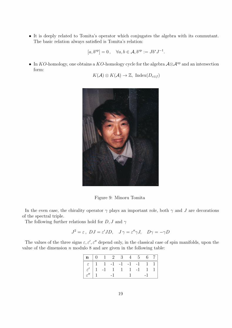
• It is deeply related to Tomita’s operator which conjugates the algebra with its commutant.The basic relation always satisfied is Tomita’s relation:

[a, bop] = 0 , ∀a, b ∈ A, bop := Jb∗J−1.

• InKO-homology, one obtains aKO-homology cycle for the algebraA⊗Aop and an intersectionform:

K(A)⊗K(A)→ Z, Index(De⊗f )

Figure 9: Minoru Tomita

In the even case, the chirality operator γ plays an important role, both γ and J are decorationsof the spectral triple.

The following further relations hold for D, J and γ

J2 = ε , DJ = ε′JD, J γ = ε′′γJ, Dγ = −γD

The values of the three signs ε, ε′, ε′′ depend only, in the classical case of spin manifolds, upon thevalue of the dimension n modulo 8 and are given in the following table:

n 0 1 2 3 4 5 6 7

ε 1 1 -1 -1 -1 -1 1 1ε′ 1 -1 1 1 1 -1 1 1ε′′ 1 -1 1 -1

19

In the classical case of spin manifolds there is a relation between the metric (or spectral) dimensiongiven by the rate of growth of the spectrum of D and the integer modulo 8 which appears in theabove table. For more general spaces, however, the two notions of dimension (the dimension modulo8 is called the “KO-dimension” because of its origin in K-theory) become independent, since thereare spaces F of metric dimension 0 but of arbitrary KO-dimension.

The search to identify the structure of the noncommutative space followed the bottom-up approachwhere the known spectrum of the fermionic particles was used to determine the geometric data thatdefines the space.

This bottom-up approach involved an interesting interplay with experiments. While at first theexperimental evidence of neutrino oscillations contradicted the first attempt, it was realized severalyears later9 in 2006 (see [19]), that the obstruction to getting neutrino oscillations was naturallyeliminated by dropping the equality between the metric dimension of space-time (which is equalto 4 as far as we know) and its KO-dimension which is only defined modulo 8. When the latteris set equal to 2 modulo 8 (using the freedom to adjust the geometry of the finite space encodingthe fine structure of space-time) everything works fine: the neutrino oscillations are there as wellas the see-saw mechanism which appears for free as an unexpected bonus. Incidentally, this alsosolved the fermion doubling problem by allowing a simultaneous Weyl-Majorana condition on thefermions to halve the degrees of freedom.

3.6 The inner fluctuations of the metric

In our joint work with A. Chamseddine and W. van Suijlekom [24], we obtained a conceptualunderstanding of the role of the gauge bosons in physics as the inner fluctuations of the metric. Iwill describe this result here in a non-technical manner.

In order to comply with Riemann’s requirement that the inverse line element D embodies theforces of nature, it is evidently important that we do not separate artificially the gravitational partfrom the gauge part, and that D encapsulates both forces in a unified manner. In the traditionalgeometrization of physics, the gravitational part specifies the metric while the gauge part corre-sponds to a connection on a principal bundle. In the NCG framework, D encapsulates both forcesin a unified manner and the gauge bosons appear as inner fluctuations of the metric but form aninseparable part of the latter. Ignoring at first the important nuance coming from the real structureJ , the inner fluctuations of the metric were first defined as the transformation

D 7→ D + A, A =∑

aj[D, bj], aj, bj ∈ A, A = A∗

which imitates the way classical gauge bosons appear as matrix-valued one-forms in the usualframework. The really important facts were that the spectral action applied to D + A delivers theEinstein-Yang-Mills action which combines gravity with matter in a natural manner, and that thegauge invariance becomes transparent at this level since an inner fluctuation coming from a gaugepotential of the form A = u[D, u∗] where u is a unitary element (i.e. uu∗ = u∗u = 1) simply resultsin a unitary conjugation D 7→ uDu∗ which does not change the spectral action.

An equally important fact which emerged very early on, is that as soon as one considers the productof an ordinary geometric space by a finite space of the simplest nature, such as two points, the inner

9This crucial step was taken independently by John Barrett

20

fluctuations generate the Higgs field and the spectral action gives the desired quartic potentialunderlying the Brout-Englert-Higgs mechanism. The inverse line element DF for the finite spaceF is given by the Yukawa coupling matrix which thus acquires geometric meaning as encoding thegeometry of F .

What we discovered in our joint work with A. Chamseddine and W. van Suijlekom [24] is thatthe inner fluctuations arise in fact from the action on metrics (i.e. the D) of a canonical semigroupPert(A) which only depends upon the algebra A and extends the unitary group. The semigroup isdefined as the self-conjugate elements:

Pert(A) := {A =∑

aj ⊗ bopj ∈ A⊗Aop |

∑ajbj = 1, θ(A) = A}

where θ is the antilinear automorphism of the algebra A⊗Aop given by

θ :∑

aj ⊗ bopj 7→

∑b∗j ⊗ a

∗opj .

The composition law in Pert(A) is the product in the algebra A⊗Aop. The action of this semigroupPert(A) on the metrics is given, for A =

∑aj ⊗ bop

j by

D 7→ D′ =AD =∑

ajDbj.

Moreover, the transitivity of inner fluctuations results fromA′(AD) =(A′A)D.

What is remarkable is that it allows one to obtain the inner fluctuations in the real case (see§3.5), i.e. in the presence of the anti-unitary involution J , without having to make the “order one”hypothesis. To do this one uses instead of the algebra A the finer one given by B = A⊗ A wherethe conjugate algebra A acts in Hilbert space using JaJ−1 for a ∈ A. The commutation of theactions of A and of A in Hilbert space ensure that B acts. One then simply defines a semigrouphomomorphism µ : Pert(A)→ Pert(B) by

A ∈ A⊗Aop 7→ µ(A) = A⊗ A ∈(A⊗ A

)⊗(A⊗ A

)op

.

This gives the inner fluctuations in the real case and they take the form

D 7→ D′ := D + A(1) + A(1) + A(2)

where, with A =∑aj ⊗ bop

j as above

A(1) =∑i

ai [D, bi]

A(1) =∑i

ai

[D, bi

], ai = JaiJ

−1, bi = JbiJ−1

A(2) =∑i,j

aiaj

[[D, bj] , bi

]=∑i,j

ai

[A(1), bi

].

The new quadratic term A(2) vanishes when the order 1 condition is fulfilled but not in general.This conceptual understanding of the inner fluctuations allowed us, with A. Chamseddine and W.van Suijlekom [24–26] to determine the inner fluctuations for the natural extension of the StandardModel obtained from the classification of irreducible finite geometries of KO-dimension 6 of [16,17].This gives a Pati-Salam extension of the Standard model and we showed in [25,26] that it yields anatural unification of couplings.

21

4 Quanta of Geometry

The above extension of the Standard Model obtained from the classification of irreducible finitegeometries of KO-dimension 6 is based on the finite dimensional algebra M2(H) ⊕M4(C). Whilethis algebra occurred as one of the simplest in the classification of [16, 17], its choice remainedmotivated by the bottom-up approach that we had followed all along up to that point. For instancethere was no conceptual explanation for the difference of the real dimensions: 16 for M2(H) and 32for M4(C).

This state of the theory changed drastically in our joint work with A. Chamseddine and S.Mukhanov [22, 23] where the above finite dimensional algebra M2(H) ⊕ M4(C) appeared unex-pectedly from a completely different motivation. The framework is the same, “spectral geometries”and the question is how to encode all spin Riemannian 4-manifolds in an operator theoretic manner.The key new idea is that since spectral triples only quantize the fundamental KO-homology classone should look at the same time for the quantization of the dual KO-theory class.

A hint of this idea can be understood easily in the one dimensional case, i.e. for the geometry ofthe circle. It is an exercise to prove that for unitary representations of the relations

UU∗ = U∗U = 1, D = D∗, U∗[D,U ] = 1 (3)

with D unbounded self-adjoint playing as above the role of the inverse line element, one has10

1. ds infinitesimal ⇒∫−|ds| ∈ N.

2. The formula d(a, b) = Sup {|f(a) − f(b)| | ‖[D, f ]‖ ≤ 1} gives the standard distance on thespectrum of U which is the unit circle in C.

3. Let M be a dimension 1 compact Riemannian manifold, (A,H, D) the associated spectraltriple. Then a solution U ∈ A of the equation U∗[D,U ] = 1 exists if and only if the length|M | ∈ 2πN.

One may understand the relations (3) as representations of a group which is a close relative of theHeisenberg group and this would lead one to group representations: but this theme would stay faraway from our goal which is 4-dimensional geometries – and which was achieved in [22,23]. What wehave discovered is a higher geometric analogue of the Heisenberg commutation relations [p, q] = i~.The role of the momentum p is played by the Dirac operator, as amply discussed above. The roleof the position variable q in the higher analogue of [p, q] = i~ was the most difficult to uncover,and another hint was given in §3.3 where the 2-sphere appeared from very simple non-commutingdiscrete variables. The general idea of [22, 23] is to encode the analogue of the position variableq in the same way as the Dirac operator encodes the components of the momenta, just using theFeynman slash. As explained below there are two levels. In the first, which is discussed in §4.1, thequantization is done for the K-theory class, and this justifies the terminology of K-theory higherHeisenberg equation. However, geometrically, the only solutions are disjoint unions of spheres ofunit volume. To reach arbitrary compact oriented spin 4-manifolds, one needs the KO-theoryrefinement. This is treated in §4.2.

10we refer to [28] for the meaning of the integral symbol

22

4.1 The K-theory higher Heisenberg equation; Spheres

Let us first rewrite the description of the algebra of §3.3, which was presented as

M2(C) ? Y, Y = Y ∗, Y 2 = 1, < Y >= 0.

As explained in §3.3 one can represent its elements as matrices with entries in the commutant ofM2(C)

Y =

(y11 y12

y21 y22

), Y =

(t zz∗ −t

)where the second form is deduced from the relations. We can rewrite the result in terms of 3 gammamatrices ΓA, 0 ≤ A ≤ 2,

Γ0 =

(1 00 −1

), Γ1 =

(0 11 0

), Γ2 =

(0 i−i 0

).

which fulfill:{ΓA,ΓB} = 2 δAB, (ΓA)∗ = ΓA

and Y now takes the simple form:

Y = Y AΓA, Y 2 = 1, Y ∗ = Y.

4.1.1 One-sided higher Heisenberg equation

This suggests the following extension for arbitrary even n. We let Y ∈ A⊗ C+ be of the Feynmanslashed form:

Y = Y AΓA, YA ∈ A, Y 2 = 1, Y ∗ = Y. (4)

Here C+ ⊂Ms(C), s = 2n/2, is an irreducible representation of the Clifford algebra on n+ 1 gammamatrices ΓA, 0 ≤ A ≤ n

ΓA ∈ C+, {ΓA,ΓB} = 2 δAB, (ΓA)∗ = ΓA.

The one-sided higher analogue of the Heisenberg commutation relations is

1

n!〈Y [D, Y ]n〉 = γ (5)

where the notation 〈T 〉 means the normalized trace of T = Tij with respect to the above matrixalgebra Ms(C) (1/s times the sum of the s diagonal terms Tii).

4.1.2 Quantization of volume

For even n, equation (5), together with the hypothesis that the eigenvalues of D grow as in dimensionn (i.e. that ds is an infinitesimal of order 1/n) imply that the volume, expressed as the leading termin the Weyl asymptotic formula for counting eigenvalues of the operator D, is quantized by beingequal to the index pairing of the operator D with the K-theory class of A defined by (note that sis even)

[e− 1/2] := [e]− s/2[1A] ∈ K0(A), e = (1 + Y )/2.

23

To understand this result, we need to recall that the integral pairing between K-homology andK-theory is computed by the pairing of the Chern characters in cyclic theory according to thediagram:

K −Theory

Ch∗

��

oo // K −Homology

Ch∗

����HC∗ oo // HC∗

While the Chern character from K-homology to cyclic cohomology is difficult, its counterpart fromK-theory to cyclic homology can be explained succinctly as follows. Given a unital (not assumedcommutative) algebra A, the (b, B)-bicomplex is obtained from the (b, B) bicomplex:

A := A/C1, Cn(A) := A⊗A⊗ · · · ⊗ A

b(a0 ⊗ · · · ⊗ an) := a0a1 ⊗ · · · ⊗ an − a0 ⊗ a1a2 ⊗ · · · ⊗ an + · · ·+(−1)n−1a0 ⊗ · · · ⊗ an−1an + (−1)nana0 ⊗ · · · ⊗ an−1

B(a0 ⊗ · · · ⊗ an) :=n∑0

(−1)nj1⊗ aj ⊗ aj+1 ⊗ · · · ⊗ aj−1.

The operations (b, B) fulfillb2 = 0, B2 = 0, bB = −Bb

and an even (resp. odd) cycle c = (cn) is given by its components cn ∈ Cn(A) for n even (resp.odd) which fulfill

Bcn + bcn+2 = 0 , ∀n even (resp. odd). (6)

The Chern character of an idempotent e ∈ A, e2 = e, is then given by the cycle with componentsCh0(e) = e ∈ A = C0(A) and for k > 0

Ch2k(e) = λk × (e− 1

2)⊗ e⊗ e⊗ · · · ⊗ e ∈ C2k(A).

One has

b(e− 1

2)⊗ e⊗ e⊗ · · · ⊗ e =

1

2(1⊗ e⊗ e⊗ · · · ⊗ e)

B(e− 1

2)⊗ e⊗ e⊗ · · · ⊗ e = B(e⊗ e⊗ e⊗ · · · ⊗ e)

= (2k + 1) (1⊗ e⊗ e⊗ · · · ⊗ e) .Thus one can choose the λk so that (2k + 1)λk + 1

2λk+1 = 0

BCh2k(e) + bCh2k+2(e) = 0

and one gets a cycle Ch∗(e) in the (b, B)-bicomplex which gives the Chen character in K-theory.In general the idempotent e does not belong to A but to matrices Ms(A) and the next step is to

pass to matrices. To do this one considers partial trace maps

tr : Cn(Ms(A))→ Cn(A).

24

One definestr : Ms(A)⊗Ms(A)⊗ · · · ⊗Ms(A)→ A⊗A⊗ · · · ⊗ A

as the linear map such that:

tr ((a0 ⊗ µ0)⊗ (a1 ⊗ µ1)⊗ · · · ⊗ (am ⊗ µm)) = Trace(µ0 · · ·µm) a0 ⊗ a1 ⊗ · · · ⊗ am

where Trace is the ordinary trace of matrices. Let us denote by ιk the operation which inserts a 1in a tensor at the k-th place. So for instance

ι0(a0 ⊗ a1 ⊗ · · · ⊗ am) = 1⊗ a0 ⊗ a1 ⊗ · · · ⊗ am

One has tr ◦ ιk = ιk ◦ tr since (taking k = 0 for instance)

tr ◦ ι0 ((a0 ⊗ µ0)⊗ (a1 ⊗ µ1)⊗ · · · ⊗ (am ⊗ µm)) =

= tr ((1⊗ 1)⊗ (a0 ⊗ µ0)⊗ (a1 ⊗ µ1)⊗ · · · ⊗ (am ⊗ µm))

= Trace(1µ0 · · ·µm)1⊗ a0 ⊗ a1 ⊗ · · · ⊗ am =

= ι0 (tr ((a0 ⊗ µ0)⊗ (a1 ⊗ µ1)⊗ · · · ⊗ (am ⊗ µm))) .

Thus the map tr induces a map tr : Cn(Ms(A))→ Cn(A) and one checks that this map is compatiblewith the operations (b, B). For an idempotent e ∈Ms(A) the components of its Chern character inC∗(A) are given by tr(Ch2k(e)). Thus they are

Ch2k(e) = λk × tr

((e− 1

2)⊗ e⊗ e⊗ · · · ⊗ e

), k > 0.

Moreover this formula still holds for k = 0 when replacing e by [e− 1/2]:

Ch2k([e− 1/2]) = λk × tr

((e− 1

2)⊗ e⊗ e⊗ · · · ⊗ e

), ∀k ≥ 0.

Using Y = 2e− 1 and the construction of the Cm(A) one thus gets, for m = 2k even,

Chm([e− 1/2]) = 2−(m+1)λktr (Y ⊗ Y ⊗ Y ⊗ · · · ⊗ Y ) ∈ Cm(A). (7)

The fundamental fact which is behind the quantization of the volume is, for Y fulfilling (4), thevanishing of all the lower components

Chm([e− 1/2]) = 0, ∀m < n. (8)

This follows because for a product P of an odd number 2k+1 < n+1 of ΓA, the trace of P vanishessince one can still find a Γ = ΓX which anti-commutes with the ΓA’s involved in P and thus

P = Γ2P = −ΓPΓ⇒ Trace(P ) = 0.

It follows from (8) that the component Chn([e− 1/2]) is a Hochschild cycle and that for any cyclicn-cocycle φn the pairing < φn, e > is the same as < I(φn),Chn(e) > where I(φn) is the Hochschildclass of φn. This applies to the cyclic n-cocycle φn which is the Chern character φn in K-homology

25

of the spectral triple (A,H, D) with grading γ where A is the algebra generated by the componentsY A of Y . One then uses the following formula for the Hochschild class τ of the Chern character φnin K-homology of the spectral triple (A,H, D), up to normalization:11

τ(a0, a1, . . . , an) =

∫−γa0[D, a1] · · · [D, an]D−n, ∀aj ∈ A.

This follows from the local index formula of Connes-Moscovici [31]. But in fact, one does not needthe technical hypothesis since, when the lower components of the operator theoretic Chern characterall vanish, one can use the non-local index formula in cyclic cohomology and the determination inthe book [28] of the Hochschild class of the index cyclic cocycle. We refer to [2] for an optimalformulation of the result. Moreover since D commutes with the algebra Ms(C) one has

τ ◦ tr(y0, y1, . . . , yn) = s

∫−γ 〈y0[D, y1] · · · [D, yn]〉D−n, ∀yj ∈Ms(A)

so that with Y = 2e− 1, one gets

< τ,Chn([e− 1/2]) >= s

∫−γ 〈Y [D, Y ]n〉D−n

and, up to normalization, equation (5) thus implies∫−D−n =

∫−γ2D−n =

1

n!

∫−γ 〈Y [D, Y ]n〉D−n =

1

n!s< τ,Chn([e− 1/2]) >∈ 1

n!sZ :

which is the quantization of the volume.

4.1.3 Disjoint Quanta

We recall that given a smooth compact oriented spin manifold M , the associated spectral triple(A,H, D) is given by the action in the Hilbert space H = L2(M,S) of L2-spinors of the algebraA = C∞(M) of smooth functions on M , and the Dirac operator D which in local coordinates is ofthe form

D = γµ(

∂

∂xµ+ ωµ

)where γµ = eµaγ

a and ωµ is the spin-connection

Theorem 4.1. Let M be a spin Riemannian manifold of even dimension n and (A,H, D) theassociated spectral triple. Then a solution of the one-sided equation (5) exists if and only if M de-composes as the disjoint sum of spheres of unit volume. On each of these irreducible components theunit volume condition is the only constraint on the Riemannian metric which is otherwise arbitraryfor each component.

11we refer to [28] for the meaning of the integral symbol

26

Figure 10: Collection of tiny spheres

Equation (4) shows that a solution Y gives a map Y : M → Sn from the manifold M to then-sphere. Let us compute the left hand side of (5). The normalized trace of the product of n + 1Gamma matrices is the totally antisymmetric tensor

〈ΓAΓB · · ·ΓL〉 = in/2εAB...L, A,B, . . . , L ∈ {1, . . . , n+ 1}.

One has

[D, Y ] = γµ∂Y A

∂xµΓA = ∇Y AΓA

where we let ∇f be the Clifford multiplication by the gradient of f . Thus one gets at any x ∈ Mthe equality

〈Y [D, Y ] · · · [D, Y ]〉 = in/2εAB...LYA∇Y B · · · ∇Y L.

Given n operators Tj ∈ C in an algebra C the multiple commutator

[T1, . . . , Tn] :=∑

ε(σ)Tσ(1) · · ·Tσ(n)

(where σ runs through all permutations of {1, . . . , n}) is a multilinear totally antisymmetric functionof the Tj ∈ C. In particular, if the Ti = ajiSj are linear combinations of n elements Sj ∈ C one gets

[T1, . . . , Tn] = Det(aji )[S1, . . . , Sn]. (9)

For fixed A, and x ∈M the sum over the other indices

εAB...LYA∇Y B · · · ∇Y L = (−1)AY A[∇Y 1,∇Y 2, . . . ,∇Y n+1]

27

where all other indices are 6= A. At x ∈M one has∇Y j = γµ∂µYj and by (9) the multi-commutator

(with ∇Y A missing) gives

[∇Y 1,∇Y 2, . . . ,∇Y n+1] = εµν...λ∂µY1 · · · ∂λY n+1[γ1, . . . , γn].

Since γµ = eµaγa and in/2[γ1, . . . , γn] = n!γ one thus gets

〈Y [D, Y ] · · · [D, Y ]〉 = n!γDet(eαa )ω

whereω = εAB...LY

A∂1YB · · · ∂nY L

so that ωdx1 ∧ · · · ∧ dxn is the pullback Y #(ρ) by the map Y : M → Sn of the rotation invariantvolume form ρ on the unit sphere Sn given by

ρ =1

n!εAB...LY

AdY B ∧ · · · ∧ dY L.

Thus, using the inverse vierbein, the one-sided equation (5) is equivalent to

det(eaµ)dx1 ∧ · · · ∧ dxn = Y #(ρ).

This equation implies that the Jacobian of the map Y : M → Sn cannot vanish anywhere, andhence that the map Y is a covering.

It would seem at this point that only disconnected geometries fit in this framework. But this wouldbe to ignore an essential piece of structure of the NCG framework, which allows one to refine (5).Namely: the real structure J , an antilinear isometry in the Hilbert space H which is the algebraiccounterpart of charge conjugation.

4.2 The KO-theory higher Heisenberg equation

We now take into account the real structure J and this gives the refinement from K to KO. Onereplaces (4) by (with summation on indices A and κ ∈ {±1})

Y = Y Aκ ΓA,κ, Y

4 = 1, Y ∗Y = 1, (10)

The Hilbert space splits according to the spectrum of Y 2 as a direct sum H = H(+)⊕H(−)

Y = Y+ ⊕ Y−, Y 2± = ±1, Y ∗± = ±Y±, Y± = Y A

± ΓA,±.

For κ ∈ {±1} the ΓA,κ fulfill in H(κ) the Clifford relations

{ΓA,κ,ΓB,κ} = 2κ δAB, (ΓA,κ)∗ = κΓA,κ.

The compatibility with J is given by the relations:

JY 2 = −Y 2J, [Y, JY J−1] = 0

28

Let C± = C(ΓA,±) be the algebra generated over R by the ΓA,κ. In H(+), C+ commutes withC ′− = JC−J

−1 to take into account the relation [Y, JY J−1] = 0. We thus view Y as a smoothsection:

Y = Y+ ⊕ Y− ∈ C∞(M,C+ ⊕ C−)

This leads us to refine the quantization condition by taking J into account as the two-sided equation

1

n!〈Z [D,Z]n〉 = γ, Z = 2EJEJ−1 − 1, [D, Y 2] = 0, (11)

where E is the spectral projection E+ ⊕ E− of the unitary Y = Y+ ⊕ Y− ∈ C∞(M,C+ ⊕ C−).

E = E+ ⊕ E− =1

2(1 + Y+)⊕ 1

2(1 + iY−)

It turns out that in dimension n = 4, the irreducible pieces give :

C+ = M2(H), C− = M4(C)

which give the algebraic constituents of the Standard Model exactly in the form of our previouswork. This can be seen using the following table:

p− q Cliffp,q(R) p− q Cliffp,q(R)mod 8 n = p+ q mod 8 n = p+ q

0 M(2n/2,R) 1 Mu(R)⊕Mu(R)u = 2(n−1)/2

2 M(2n/2,R) 3 M(2(n−1)/2,C)

4 M(2(n−2)/2,H) 5 Mv(H)⊕Mv(H)v = 2(n−3)/2

6 M(2(n−2)/2,H) 7 M(2(n−1)/2,C)

Indeed in dimension n = 4 one needs n + 1 = 5 gamma matrices, and the irreducible pieces of theClifford algebras Cliffp,q(R) are M2(H) for (p, q) = (5, 0) and M4(C) for (p, q) = (0, 5). Moreover inthe 4-dimensional case one has, in the Hilbert space H(+), by the detailed calculation of [23],⟨

Z [D,Z]4⟩

+=

1

2

⟨Y+ [D, Y+]4

⟩+

1

2

⟨Y ′−[D, Y ′−

]4⟩,

where Y ′− = iJY−J−1. One now gets two maps Y± : M → Sn while (11) becomes, up to normaliza-

tiondet(eaµ)dx1 ∧ · · · ∧ dxn = Y #

+ (ρ) + Y #− (ρ), (12)

29

where Y #± (ρ) is the pull back of the volume form ρ of the sphere.

For an n-dimensional smooth compact manifold we let D(M) be the set of pairs of smooth mapsφ± : M → Sn such that the differential form

φ#+(ρ) + φ#

−(ρ) = ω

does not vanish anywhere on M (ρ is the standard volume form on the sphere Sn).

Definition 4.2. Let M be an n-dimensional oriented smooth compact manifold

qM := {deg(φ+) + deg(φ−) | (φ+, φ−) ∈ D(M)}

where deg(φ) is the topological degree of φ.

Theorem 4.3. (i) Let M be a compact oriented spin Riemannian manifold of dimension 4. Then asolution of (12) exists if and only if the volume of M is quantized to belong to the invariant qM ⊂ Z.(ii) Let M be a smooth connected oriented compact spin 4-manifold. Then qM contains all integersm ≥ 5.

The invariant qM makes sense in any dimension. For n = 2, 3, and any M , it contains all sufficientlylarge integers. The case n = 4 is more difficult; but we showed in [23] that for any Spin manifold itcontains all integers m > 4. This uses fine results on the existence of ramified covers of the sphereand on immersion theory going back to Smale, Milnor and Poenaru. By a result of M. Iori, R.Piergallini [37], any orientable closed (connected) smooth 4-manifold is a simple 5-fold cover of S4

branched over a smooth surface (meaning that the covering map can be assumed to be smooth).The key lemma12 which allows one to then rely on immersion theory and apply the fundamentalresult of Poenaru [43] (on the existence of an immersion in Rn of any open parallelizable n-manifold)is the following:

Lemma 4.4. Let φ : M → S4 be a smooth map such that φ#(α)(x) ≥ 0 ∀x ∈M and let R = {x ∈M | φ#(α)(x) = 0}. Then there exists a map φ′ such that φ#(α) +φ′#(α) does not vanish anywhereif and only if there exists an immersion f : V → R4 of a neighborhood V of R. Moreover if thiscondition is fulfilled one can choose φ′ to be of degree 0.

The spin condition on the 4-manifold allows one to prove that the neighborhood V is parallelizable.By a result of A. Haefliger, the spin condition is equivalent to the vanishing of the second Stiefel-Whitney class w2 of the tangent bundle. In the converse direction, Jean-Claude Sikorav and BrunoSevennec found the following obstruction which implies for instance that D(CP 2) = ∅. Let M be anoriented compact smooth 4-dimensional manifold, then, with w2 the second Stiefel-Whitney classof the tangent bundle,

D(M) 6= ∅ =⇒ w22 = 0

Indeed if D(M) 6= ∅ one has a cover of M by two open sets on which the tangent bundle is stablytrivialized. Thus the above product of two Stiefel-Whitney classes vanishes.

12I am indebted to Simon Donaldson for his generous help in finding this key result

30

Figure 11: Ramified cover of the sphere

4.3 Emerging Geometry

Theorem 4.3 shows how 4-dimensional spin geometries arise from irreducible representations ofsimple algebraic relations. There is no restriction to fix the Hilbert space H as well as the actions ofthe Clifford algebras C± and of J and γ. The remaining indeterminate operators are D and Y . Theyfulfill equation (11). The geometry appears from the joint spectrum of the Y A

± and is a 4-dimensionalimmersed submanifold in the 8-dimensional product S4×S4. Thus this suggests taking the operatorsY,D as being the correct variables for a first shot at a theory of quantum gravity. In the sequelthe algebraic relations between Y±, D, J , C±, γ are assumed to hold. As we have seen above acompact spin 4-dimensional manifold M appears as immersed by a map (Y+, Y−) : M → S4 × S4.An interesting question which comes in this respect is whether, given a compact spin 4-dimensionalmanifold M , one can find a map (Y+, Y−) : M → S4 × S4 which embeds M as a submanifold ofS4× S4. One has the strong Whitney embedding theorem: M4 ⊂ R4×R4 ⊂ S4× S4 so there is noa-priori obstruction to expect an embedding rather than an immersion. It is worthwhile to mentionthat a generic immersion would in fact suffice to reconstruct the manifold. Next, in general, if onestarts from a representation of the algebraic relations, there are two natural questions:

A): Is it true that the joint spectrum of the Y A+ and Y B

− is of dimension 4 while one has 8 variables?

B): Is it true that the volume∫−D−4 remains quantized?

4.3.1 Dimension

The reason why A) holds in the case of classical manifolds is that in that case the joint spectrumof the Y A and Y ′B is the subset of S4 × S4 which is the image of the manifold M by the mapx ∈M 7→ (Y (x), Y ′(x)) and thus its dimension is at most 4.

31

The reason why A) holds in general is because of the assumed boundedness of the commutators[D, Y ] and [D, Y ′] together with the commutativity [Y, Y ′] = 0 (order zero condition) and the factthat the spectrum of D grows like in dimension 4.

4.3.2 Quantization of volume

The reason why B) holds in the general case is that the results of §4.1.2 apply separately to Y+ andY ′−. This gives, up to a normalization constant c4 6= 0, the integrality∫

−γ⟨Y+ [D, Y+]4

⟩D−4 = c4 < [D], [e− 1/2] >∈ c4 Z∫

−γ⟨Y ′−[D, Y ′−

]4⟩D−4 = c4 < [D], [e′ − 1/2] >∈ c4 Z.

Thus the equality ⟨Z [D,Z]4

⟩+

=1

2

⟨Y+ [D, Y+]4

⟩+

1

2

⟨Y ′−[D, Y ′−

]4⟩.

together with equation (11) gives in H(+),

1

2

⟨Y+ [D, Y+]4

⟩+

1

2

⟨Y ′−[D, Y ′−

]4⟩= 4!γ

and one gets from γ2 = 1:

Theorem 4.5. In any operator representation of the two sided equation (11) in which the spectrumof D grows as in dimension 4 the volume (the leading term of the Weyl asymptotic formula) isquantized, (up to a normalization constant c > 0)∫

−D−4 ∈ cN.

This quantization of the volume implies that the bothersome cosmological leading term of thespectral action is now quantized; and thus it no longer appears in the differential variation of thespectral action. Thus and provided one understands better how to reinstate all the fine details ofthe finite geometry (the one encoded by the Clifford algebras) the variation of the spectral actionwill reproduce the Einstein equations coupled with matter.

4.4 Final remarks

Finally, we briefly discuss a few important points which would require more work of clarification ifone wants to get a bit closer to the goal of unification at the “pre-quantum” level, best describedin Einstein’s words (see H. Nicolai, Cern Courier, January 2017) as follows:

“Roughly but truthfully, one might say: we not only want to understand how nature works, butwe are also after the perhaps utopian and presumptuous goal of understanding why nature is theway it is and not otherwise.”

32

1. All our discussion of geometry takes place in the Euclidean signature. Physics takes placein the Minkowski signature. The Wick rotation plays a key role in giving a mathematicalmeaning to the Feynman integral in QFT for flat space-time but becomes problematic forcurved space-time. But following Hawking and Gibbons one can investigate the EuclideanFeynman integral over compact 4-manifolds implementing a cobordism between two fixed 3-geometries. Two interesting points occur if one uses the above spectral approach. First thenew boundary terms, involving the extrinsic curvature of the boundary, which Hawking andGibbons had to add to the Einstein action, pop up automatically from the spectral action:as shown in [18]. Second, in the functional integral, the kinetic term of the Weyl term (i.e.the “dilaton”) has the wrong sign. In our formalism the higher Heisenberg equation fixes thevolume form and automatically freezes the dilaton.

2. The number of generations is not predicted by the above theory. The need to have thismultiplicity in the representation of the finite algebra AF might be related to the discussionof §3.4 in the following way. For non-simply connected spaces the Poincare duality KO-fundamental class should take into account the fundamental group. We skipped over thispoint in §3.4; and in the non-simply connected case one needs to twist the fundamental KO-homology class by flat bundles. It is conceivable that the generations appear from such a twistby a 3-dimensional representation. This could be a good motivation to extend the classicaltreatment of flat bundles (i.e. of representations of the fundamental group) to the general caseof noncommutative spaces.

5 Appendix

Here is a possible translation of the second quote of Grothendieck:It must be already fifteen or twenty years ago that, leafing through the modest volume constitut-

ing the complete works of Riemann, I was struck by a remark of his “in passing”. He pointed outthat it could well be that the ultimate structure of space is discrete, while the continuous represen-tations that we make of it constitute perhaps a simplification (perhaps excessive, in the long run...) of a more complex reality; That for the human mind, “the continuous” was easier to graspthan “the discontinuous”, and that it serves us, therefore, as an “approximation” to apprehend thediscontinuous.

This is a remark of a surprising penetration in the mouth of a mathematician, at a time whenthe Euclidean model of physical space had never yet been questioned; in the strictly logical sense,it is rather the discontinuous which traditionally served as a mode of technical approach to thecontinuous.

Mathematical developments of recent decades have, moreover, shown a much more intimate sym-biosis between continuous and discontinuous structures than was imagined, even in the first half ofthis century.

In any case finding a “satisfactory” model (or, if necessary, a set of such models, “satisfactorilyconnecting” to each other) of “continuous”,“discrete” or of “mixed” nature - such work will surelyinvolve a great conceptual imagination, and a consummate flair for apprehending and unveiling newtype mathematical structures.

This kind of imagination or “flair” seems rare to me, not only among physicists (where Einstein

33

and Schrodinger seem to have been among the rare exceptions), but even among mathematicians(and here I speak with full knowledge).

To summarize I predict that the expected renewal (if it must yet come) will come from a math-ematician in soul well informed about the great problems of physics, rather than from a physicist.But above all, it will take a man with “philosophical openness” to grasp the crux of the problem.This is by no means a technical one but rather a fundamental problem of natural philosophy.”

References

[1] M. Atiyah Global theory of elliptic operators. 1970 Proc. Internat. Conf. on Functional Analysisand Related Topics (Tokyo, 1969) pp. 2130 Univ. of Tokyo Press, Tokyo

[2] A. Carey, A. Rennie, F. Sukochev, D. Zanin, Universal measurability and the Hochschild classof the Chern character. J. Spectr. Theory 6 (2016), no. 1, 1–41.

[3] http://acces.ens-lyon.fr/clea/lunap/Triangulation/TriangCompl1.html

[4] A. Chamseddine, A. Connes, Universal formula for noncommutative geometry actions: unifi-cation of gravity and the Standard Model, Phys. Rev. Lett. 77, 486804871 (1996).

[5] A. Chamseddine, A. Connes, The Spectral action principle, Comm. Math. Phys. Vol.186 (1997),731–750.

[6] A. Chamseddine, A. Connes, Scale invariance in the spectral action, J. Math. Phys. 47 (2006),N.6, 063504, 19 pp.

[7] A. Chamseddine, A. Connes, Inner fluctuations of the spectral action, J. Geom. Phys. 57 (2006),N.1, 1–21.

[8] A. Chamseddine, A. Connes, Why the Standard Model, hep-th 0706.3688.

[9] A. Chamseddine, A. Connes, A dress for SM the beggar, hep-th 0706.3690.

[10] A. Chamseddine, A. Connes, Quantum gravity boundary terms from the spectral action ofnoncommutative space, Phys. Rev. Letter LE11230, hep-th 0705.1786.

[11] A. Chamseddine, A. Connes, M. Marcolli, Gravity and the standard model with neutrino mixing,hep-th/0610241.

[12] A. Chamseddine, A. Connes, Universal formula for noncommutative geometry actions: unifi-cation of gravity and the Standard Model, Phys. Rev. Lett. 77, 486804871 (1996).

[13] A. Chamseddine, A. Connes, The Spectral action principle, Comm. Math. Phys. Vol.186 (1997),731–750.

[14] A. Chamseddine, A. Connes, Scale invariance in the spectral action, J. Math. Phys. 47 (2006),N.6, 063504, 19 pp.

34

[15] A. Chamseddine, A. Connes, Inner fluctuations of the spectral action, J. Geom. Phys. 57 (2006),N.1, 1–21.

[16] A. Chamseddine, A. Connes, Why the Standard Model?, hep-th 0706.3688.

[17] A. Chamseddine, A. Connes, A dress for SM the beggar, hep-th 0706.3690.

[18] A. Chamseddine, A. Connes, Quantum gravity boundary terms from the spectral action ofnoncommutative space, Phys. Rev. Letter LE11230, hep-th 0705.1786.

[19] A. Chamseddine, A. Connes, M. Marcolli, Gravity and the standard model with neutrino mixing,hep-th/0610241.

[20] A. Chamseddine and A. Connes, Noncommutative Geometry as a framework for unification ofall fundamental interactions including gravity. Fortsch. Phys. 58 (2010) 553.

[21] A. Chamseddine and A. Connes, Resilience of the Spectral Standard Model, JHEP, 1209 (2012)104.

[22] A. Chamseddine, A. Connes and V. Mukhanov, Quanta of Geometry: Noncommutative Aspects,Phys. Rev. Lett. 114 (2015)

[23] A. Chamseddine, A. Connes and V. Mukhanov, Geometry and the Quantum: Basics, JHEP12 (2014) 098.

[24] A. Chamseddine, A. Connes and W. D. van Suijlekom, Inner Fluctuations in NoncommutativeGeometry without the First Order Condition. Jour. Geom. Phys. 73 (2013) 222.

[25] A. Chamseddine, A. Connes and W. D. van Suijlekom, Beyond the Spectral Standard Model:Emergence of Pati-Salam Unification. JHEP 11 (2013) 132.

[26] A. Chamseddine, A. Connes and W. D. van Suijlekom, Grand Unification in the Spectral Pati-Salam models. JHEP 2511 (2015) 011.

[27] A. Connes, Lecon inaugurale au College de France. 11 Janvier 1985.http://www.alainconnes.org/docs/lecollege.pdf

[28] A. Connes, Noncommutative geometry, Academic Press (1994).

[29] A. Connes. C∗-algebres et geometrie differentielle. C.R. Acad. Sci. Paris Ser. A-B 290 (1980),A599-A604.

[30] A. Connes. Noncommutative geometry and reality. Journal of Mathematical Physics 36, 6194(1998)

[31] A. Connes, H. Moscovici, The local index formula in noncommutative geometry, GAFA, Vol. 5(1995), 174–243.

[32] L. Corry David Hilbert and the axiomatization of physics. Springer-Science + Business-MediaB.V. (2004).

35

[33] B. Dundas, T. Goodwillie, R. McCarthy, The local structure of algebraic K-theory. Algebra andApplications, 18. Springer-Verlag London, Ltd., London, 2013.

[34] N. Gisin, A. Martin, B. Sanguinetti, H. Zbinden, Quantum random number generation on amobile phone, Phys. Rev. X 4, 031056 (2014)

[35] A. Grothendieck, Recoltes et Semailles.

[36] T. Hankins, Sir William Rowan Hamilton. Johns Hopkins University Press, Baltimore, Md.,1980.

[37] M. Iori, R. Piergallini, 4-manifolds as covers of the 4-sphere branched over non-singular sur-faces. Geometry and Topology, 6 (2002) 393–401.

[38] J. Kouneiher, J. Stachel, Einstein and Hilbert. In this volume.

[39] C. MacLarty, Grothendieck on foundations for the rebirth of geometry. In this volume.

[40] J. Milnor, J. Stasheff, Characteristic classes. Annals of Mathematics Studies, No. 76. PrincetonUniversity Press, Princeton, N. J.; University of Tokyo Press, Tokyo, 1974.

[41] J. Moser, On the volume elements on a manifold. Trans. Amer. Math. Soc. 120 1965 286–294.

[42] A. Pais, Inward Bound: Of Matter and Forces in the Physical World. Oxford University Press(1986)

[43] V. Poenaru, Sur la theorie des immersions. Topology 1 (1962) 81–100.

[44] P. H. Siegel Witt Spaces: A Geometric Cycle Theory for KO-Homology at Odd Primes. Amer-ican Journal of Mathematics Vol. 105, No. 5 (Oct., 1983), pp. 1067–1105

[45] I. Singer Future extensions of index theory and elliptic operators Prospects in mathematics.Ann. of Math. Studies 70. Princeton Univ. Press (1971), 171–185.

[46] M. Spivak Spaces satisfying Poincare duality. Topology 6 1967 77–101.

[47] R. P. Woodard How far are we from the quantum theory of gravity? Rep. Progr. Phys. 72(2009), no. 12, 126002, 42 pp. 81V17 (83C45)

36