geometry and mechanics - core.ac.uk vascular blood ﬂow with the purpose of designing predictive...

For multiple-author papers: Contact author designated by * Presenting author designated by underscore

Geometry and Mechanics Session Organizers: Kai-Uwe BLETZINGER (TU Munich), Fehmi CIRAK (University of Cambridge) Keynote Lecture Modeling and computation of patient-specific vascular fluid-structure interaction using Isogeometric Analysis Yuri BAZILEVS*, Victor M. CALO, Thomas J. R. HUGHES (University of Texas at Austin), Yongie ZHANG (Carnegie Mellon University) Keynote Lecture Optimal shapes of mechanically motivated surfaces Kai-Uwe BLETZINGER*, Matthias FIRL, Johannes LINHARD, Roland WÜCHNER (TU Munich) Subdivision shells for nonsmooth and branching geometries Quan LONG, Fehmi CIRAK* (University of Cambridge) Water landing analyses with explicit finite element method John T. WANG (NASA Langley Research Center) On a geometrically exact contact description for shells: From linear approximations for shells to high-order FEM Alexander KONYUKHOV, Karl SCHWEIZERHOF* (University of Karlsruhe)

Proceedings of the 6th International Conference onComputation of Shell and Spatial Structures

IASS-IACM 2008: ”Spanning Nano to Mega”28-31 May, 2008, Cornell University, Ithaca, NY, USA

John F. ABEL and J. Robert COOKE (eds.)

Modeling and computation of patient-specific vascularfluid-structure interaction using Isogeometric Analysis

Yuri Bazilevs∗, Victor M. Calo, Thomas J.R. Hughes, and Yongie Zhang

*Institute for Computational Engineering and Sciences (ICES)The University of Texas at Austin201 E. 24th street, Austin, TX 78712, [email protected]

1 Introduction

Cardiovascular disease is the number one killer of men and women in the US and is the primary cause ofcongestive heart failure (CHF), which afflicts over 4.7 million Americans. There are 550,000 new cases ofCHF reported annually. Cardiovascular disease produces a number of physiological changes to the tissuesof the cardiovascular system (e.g., loss of elasticity of the arteries as in arteriosclerosis, ischemic damageand cardiomyopathies). These change the hemodynamics of the cardiovascular system with potentiallydisastrous consequences. The geometric and physical complexity of the human cardiovascular system andthe limited possibility to perform experiments and measurement opened doors for computational analysisof vascular blood flow with the purpose of designing predictive tools for treatment planning or evaluationof assist devices for individual patients. The concept of patient-specific cardiovascular modeling was firstestablished in Taylor et al. [1], where real-life geometries were used to simulate blood flow. In thelast decade, the computational technology has experienced further advances, which includes simulatingmore complicated geometries corresponding to larger and larger portions of the cardiovascular system,accounting for arterial wall elasticity, heart valves, and growth and remodeling of arterial tissue.

Recently, Isogeometric Analysis has emerged as a new computational technology and as an alternativeto the standard finite element method (see Hughes et al. [2]). Isogeometric analysis improves uponfinite elements in the areas of geometric modeling and solution representation. The first instantiationof isogeometric analysis was based upon Non-Uniform Rational B-Splines (NURBS), although otheralternatives, such as subdivision and T-Splines, are possible and are currently under investigation. Despiteits recent emergence, NURBS-based isogeometric analysis has already been applied to many areas ofcontemporary interest in computational mechanics. These include: fluids and turbulence, solids andthin structures, fluid-structure interaction and, recently, phase-field modeling. Improved geometry andsolution approximation properties of NURBS functions has led to superior performance of the isogeometricapproach in comparison to standard finite elements in these applications.

In this paper, isogeometric analysis is applied to fluid-structure interaction (FSI) problems with

1

6th International Conference on Computation of Shell and Spatial Structures IASS/IACM 2008, Ithaca

particular emphasis on arterial modeling and blood flow. It is believed that the ability of NURBS toaccurately represent smooth exact geometries, that are natural for arterial systems, but unattainablein the faceted finite-element representation, and the high order of approximation of NURBS, renderfluid and structural computations more physiologically realistic. This work adopts the ALE framework.The arterial wall is treated as a nonlinear hyperelastic solid in the Lagrangian description governed bythe equations of elastodynamics. Blood is assumed to be a Newtonian viscous fluid governed by theincompressible Navier-Stokes equations written in the arbitrary Lagrangian-Eulerian form. The fluidvelocity is set equal to the velocity of the solid at the fluid-solid interface. The coupled FSI problem iswritten in a variational form such that the stress compatibility condition at the fluid-solid interface isenforced weakly. Because our aim in this work is to obtain a robust isogeometric analysis formulation forfluid-structure interaction, we opted for a monolithic approach to solving the coupled equation systemthat we further developed in Bazilevs et al. [3].

The paper is organized as follows. In Section 2 we present and make an assessment of the solidmodel describing the behavior of arterial wall tissue. In Section 3 we present results of the fluid-structureinteraction calculation of a patient-specific abdominal aortic aneurysm.

2 Investigation of the solid model for a range of physiological stresses

(a) (b)

Figure 1: (a) Setup for a uniaxial stress state. (b) Equilibrium on a cylinder with imposed internalpressure.

The arterial wall is modeled as a hyperelastic solid for which the elastic potential ψ is given by (seeSimo and Hughes [4])

ψ =1

2µs(trC − 3) +

1

2κs(

1

2(J2

− 1) − lnJ), (1)

where C = FTF, F = J−1/3

F, F is the deformation gradient and J is its determinant, and µs and κs arethe shear and bulk moduli, respectively. We examine the behavior of the material model (1) on a simplestate of uniaxial stress. We consider a bar with an applied stress in the x-direction, denoted by σ, andzero stress in the the orthogonal directions, as illustrated in Figure 1(a).

The relevant values of σ corresponding to the physiologically-realistic range of intramural pressure areobtained using the following analysis. We approximate the arterial cross-section as a hollow cylinder. LetRi and Ro denote its inner and outer radii. We also assume that a pressure of magnitude p0 is appliedat the inner wall of the cylinder, as shown in Figure 1(b). We assume an approximately constant stateof stress through the thickness. From force equilibrium considerations it follows that

2Rip0 = 2σt (2)

2


0 0.05 0.1 0.15 0.2 0.25 0.3 0.35 0.4 0.450

1000

1500

2000

2500

533

800

Strain: (lx−l

0x)/l

x

Cau

chy

stre

ss (

mm

Hg)

Physiological stress range due to intramural pressure

Tangent modulus at zero stress: 4.14x106 dyn/cm2 or 3.11x103 mmHg

Tangent modulus at physiological stress:6.00x106 dyn/cm2 or 4.50x103 mmHg

Figure 2: Cauchy stress plotted against strain. Physiological range of stresses and strains due to intra-mural pressure are indicated by dashed lines.

where t = Ro −Ri is the thickness of the arterial wall. Solving for σ, we get

σ = p0Ri/t. (3)

Assuming µs = 1.43 × 106 dyn/(cm2) and κs = 1.38 × 107 dyn/(cm2), a thickness-to-radius ratio of15%, and p0 varying from 80 mmHg to 120 mmHg, we get the physiologically-realistic stress rangingfrom approximately 530 mmHg to 800 mmHg. The stress-strain curve is plotted in Figure 2. Notethat the stress-strain curve exhibits a superlinear behavior throughout the range of loadings considered,showing stiffening with deformation. Also note that for the physiological range of stresses the deviationfrom linearized stress-strain relationship is not significant. Obviously, significant improvements are pos-sible. However, the present model is both qualitatively and quantitatively reasonable for the followingapplication.

3 Flow in a patient-specific abdominal aortic aneurysm

We present results of the fluid-structure interaction calculation of a patient-specific abdominal aorticaneurysm. Patient-specific geometry is obtained from 64-slice CT angiography courtesy of T. Kvamsdaland J.H. Kaspersen of SINTEF, Norway. The computational mesh, consists of 44892 quadratic NURBSelements. Two quadratic NURBS elements and four C1-continuous basis functions are used for through-thickness resolution of the arterial wall. A periodic flow waveform, with period T = 1.05 s, is applied atthe inlet of the aorta, while resistance boundary conditions are applied at all outlets. The solid is fixedat the inlet and at all outlets. Material and flow rate data, as well as resistance values are taken fromFigueroa et al. [5]. We compute with the time-varying inflow boundary condition until periodic-in-timeresponse is attained. This usually takes four or five cycles.

Figure 3 shows snapshots of the velocity field plotted on the moving domain at various times duringthe heart cycle. The flow field is quite complex and fully three-dimensional, especially in diastole. Figure4(a) shows the magnitude of the wall shear stress (i.e., the tangential component of the fluid (or solid)traction vector) averaged over a cycle. Note that the wall shear stress is significantly lower in the aneurysmregion than in the upper portion of the aorta and at branches. Also note the smoothness of the stresscontours due to the NURBS representation of the geometry and solution fields. Figure 4(b) shows theoscillatory shear index (OSI), which is a measure of variability of the wall shear stress over a heart beat.In contrast to the wall shear stress, OSI is largest in the aneurysm region, especially along the posteriorwall, suggesting that wall shear stress is highly oscillatory there due to the recirculating flow. Low time-averaged wall shear stress in combination with high shear stress temporal oscillations are indicators of

3


(a) t = 4/25 T (b) t = 10/25 T

Figure 3: Flow in a patient-specific abdominal aorta with aneurysm. Large frame: fluid velocity vectorscolored by their magnitude and detail of the top portion of the artery. Left small frame: volume renderingof the velocity magnitude. Right small frame: fluid velocity isosurfaces.

(a) (b)

Figure 4: Flow in a patient-specific abdominal aorta with aneurysm. (a) Magnitude of wall shear stressaveraged over a cycle plotted in three different views. (b) Oscillatory shear index (OSI) plotted in threedifferent views.

the regions of high probability of occurrence of atherosclerotic disease.

References

[1] Taylor CA, Hughes TJR, Zarins CK. Finite element modeling of blood flow in arteries Computer

Methods in Applied Mechanics and Engineering 1998; 158:155–196.

[2] Hughes TJR, Cottrell JA, Bazilevs Y. Isogeometric analysis: CAD, finite elements, NURBS, ex-act geometry, and mesh refinement Computer Methods in Applied Mechanics and Engineering 2005;194:4135–4195.

[3] Bazilevs Y, Calo VM, Hughes TJR, Zhang Y. A fully-integrated approach to fluid-structure interactionanalysis Computational Mechanics 2008; Submitted

[4] Simo JC and Hughes TJR. Computational Inelasticity Springer-Verlag, 1998.

[5] Figueroa A, Vignon-Clementel IE, Jansen KE, Hughes TJR, Taylor CA. A coupled momentum methodfor modeling blood flow in three-dimensional deformable arteries Computer Methods in Applied Me-

chanics and Engineering 2006; 195:5685–5706.

4

Proceedings of the 6th International Conference on

Computation of Shell and Spatial Structures IASS-IACM 2008: “Spanning Nano to Mega”

28-31 May 2008, Cornell University, Ithaca, NY, USA John F. ABEL and J. Robert COOKE (eds.)

1

Optimal shapes of mechanically motivated surfaces Kai-Uwe BLETZINGER*, Matthias FIRL, Johannes LINHARD and Roland WÜCHNER

*Lehrstuhl für Statik, Technische Universität München Arcisstr. 21, D-80333 München, Germany [email protected]

Abstract Subject of this contribution is form finding of “optimal” structural shapes with regard to the load carrying behaviour of surface structures under certain load cases. In general, those optimal shapes prefer a membrane state of stress to transfer loading. Bending is omitted as much as possible. It will be focused on two different disciplines and related numerical approaches which deal with solutions of the mentioned task: form finding of pre-stressed membranes and general shape optimization. As design is an inverse problem both approaches share similar problematic properties as e.g. indeterminate in-plane location of surface discretization or necessary regularization and filtering of sensitivity and other data. As it will turn out, those remedies found for the very special methods of membrane design can be abstracted and transferred to general optimization procedures. That merges into elegant, numerical shape optimal design techniques which combine advantages of both approaches and allow for effective and efficient shape optimization of free formed surfaces, directly on the finite element mesh and for a large number of variables. Typical applications are, for example, membrane design, free form architecture and structural engineering, and metal sheet design.

1. Form finding of surface structures with membrane action The geometry of membrane structures is defined by “form finding” as the equilibrium shape of given surface and edge cable stresses σ and additional surface loading q.

Figure 1: Form finding of membrane

The equilibrium surface can be identified as actual (deformed) configuration, which has to fulfil the equilibrium condition governed by the principle of virtual work:

( ) 0 =⋅−=− ∫∫4342144 344 21

external

a

ernalint

a

dada:tw uqxu δ

∂δ∂δ σ (1)

6th International Conference on Computation of Shell and Spatial Structures IASS-IACM 2008, Ithaca

The total virtual work δw can be separated into two parts: The internal work resulting from the given internal Cauchy stresses σ and the derivatives of virtual displacements δu with respect to the material points x of the equilibrium surface, and the external virtual work due to the virtual displacements of the external loading q. At this point, no restrictions concerning the load case are made and even deformation dependent loads (e.g. pressure loads) can be consistently considered. The integration domain is the area a of the final surface. Thickness t is assumed to be constant during deformation.

Eq. (1) might be transformed by standard pull back operation to the reference configuration:

( ) ( )( ) 0 1 =⋅⋅⋅==− ∫∫ −−−

dA:dettda:twA

Tbackpull

aint FFσFFF

xuσ δ

∂δ∂δ (2)

Integration domain is now the area A of the known reference configuration. F is the deformation gradient.

Note: The shape is defined by equilibrium of given stress fields. As no material law is defined stress is independent from strain. As a consequence standard application of discretization results in singular, non-linear systems of equations. That is the typical property of an inverse problem. It might be graphically explained by the fact that discretization nodes can be moved around on the corresponding equilibrium surface without resistance while still maintaining a valid discretization of the sought-after surface, i.e. Eq. (1) is always fulfilled. To overcome this problem, many different strategies were developed over the years. In the following, a method which is consistently derived from nonlinear continuum mechanics is presented.

Figure 2: Alternative surface discretization: “Floating” mesh for hypar-like membrane structure

2.1 Regularization of inverse problem First, the Cauchy stress tensor σ is expressed by the 2nd Piola-Kirchhoff stress tensor S. We get from Eq. (2):

( )( ) ( ) 0 1 =⋅=⋅⋅⋅=− ∫∫ −− dA:tdA:dettwAA

Tint FSFFFσFFF δδδ (3)

Since the intensity of Cauchy surface stress is given, Piola Kirchhoff stresses are a function of deformation.

Second, now, the intensity of Piola Kirchhoff surface stress is prescribed by S with respect to the choice of a suitable reference configuration. Consequently, Cauchy stresses are now a function of deformation and we solve a similar but slightly different problem which, however, is not singular anymore:

( ) 0 =⋅=−=− ∫ dA:ˆtwJA

int FSF δδδ (4)

The original problem might be regularized by adding some portion of Eq. (4) to Eq. (3), weighted by homotopy factor λ which might be chosen appropriately:

2


( ) 0 1 =−−−=− intintint www~ δλδλδ (5)

Choice of λ = 1 might be interpreted as the generalized force density method.

2.2 Updated reference strategy, URS Solution of Eq. (5) might be used as “updated” reference configuration for a next solution. Subsequently applied the procedure will converge to a solution of the original problem, Eq. (2). That holds for the extreme case of λ = 1 also. Additional considerations are necessary for anisotropic pre-stresses or special boundary conditions.

2.3 Examples of pre-stressed surfaces applying URS

Figure 3: Five point tent; given surface stress and edge cable pre-stress

Figure 4: Form finding of an air supported cushion; prescribed surface stress and internal pressure

Figure 5: Form finding of compression dome under snow loading and fixed edges (λmax refers to additional

means of mesh control indicating anisotropic stress fields at the solution)

3. Shape optimization Alternatively to form finding, most general shape optimal design procedures are defined by minimization of an objective f (e.g. strain energy, weight etc.) with respect to design variables s subject to constraints g and h:

( )( )( )

⎪⎩

⎪⎨

⎧

≤≤=≤

→ul

),(h),(g

.t.smin),(fsss

ssxssx

ssx 00

(6)

Geometry x is a function of design variables s. The most general situation is defined by directly identifying coordinates of the FE mesh as design variables. As a consequence that formulation must be regularized with respect to in-plane and out-of-plane design modification, again because of inverse problem characteristics.

3


3.1 In-plane Regularization Except for discretization errors objective functions f are independent from surface discretization. That is the same phenomenon as shown in Fig. (2). As a consequence the optimization problem must be regularized for in-plane modification of surface discretization. That can be done in abstract notation by adding a stabilizing term

( ) ( ) ( )( ) minJfsf~ →+= sPs (7)

to the objective function. The variation of functional J is related to geometrical modification tangential to the structural surface, refer to Eq. (4). J is defined by an artificial surface stress field used to generate a smooth mesh. P is a projection operator which is defined by the surface normal n and which determines the tangential action of design modification.

3.2 Out-of-plane Regularization To prevent mesh dependent results when directly using finite element coordinates as design variables additional filter methods are applied. Consider response f at node m. Then, the sensitivity of f with respect to a design variable s is computed by:

∑

∑

=

= ∂∂

⋅=

∂∂

n

ip

i

n

ip

im

DsfD

sf

1

1 (8)

piD is the value of filter function of order p at node i which is defined inside a given, mesh independent filter

radius. The most simple choice of a filter is a linear decreasing, radial hat function (p = 1).

3.3 Example A bend cantilever made of a thin (metal) sheet is loaded as shown, Fig. 6. Shape is modified to maximize stiffness. A filter radius as large as the width of support is used. The model consists of appr. 5.000 shape variables. The optimal shape (most right) is reached after 19 iteration steps.

Figure 6: Shape optimization of cantilever shell.

References [1] Bletzinger K-U, Wüchner R, Daoud F, Camprubí N. Computational methods for form finding and

optimization of shells and membranes. Comp. Methods Appl. Mech. Engrg. 2005; 194: 3438-3452. [2] Bletzinger K-U, Firl M, Daoud F. Approximation of Derivatives in Semi-Analytical Structural

Optimization. In proc. of III. European Conference on Computational Mechanics, C.A. Mota Soares et.al. (eds), Lisbon Portugal, 2006.

[3] Linhard J, Wüchner R., Bletzinger K-U. “Upgrading” membranes to shells—The CEG rotation free shell element and its application in structural analysis. Finite Elements in Analysis and Design 2007; 44: 63– 74.

[4] Wüchner R, Bletzinger K-U. Stress-adapted numerical form finding of pre-stressed surfaces by the updated reference strategy. Int. J. Numer. Methods Engrg. 2005; 64: 143-166.

4




Subdivision shells for nonsmooth and branching geometries

Quan LONG* and Fehmi CIRAK

*Department of Engineering, University of Cambridge Trumpington Street , Cambridge CB2 1PZ , UK [email protected], http://www-g.eng.cam.ac.uk/csml/

Abstract In [2, 3, 4] we had introduced the iso-geometric subdivision elements for discretising thin-shell energy functionals that require smooth shape functions. In the present work we have extended the subdivision elements to shells with non-smooth reference configurations and shells with intersections. Furthermore, the new elements simplify the enforcement of displacement, rotation, traction and moment boundary conditions. In our original approach we had used ghost nodes at the boundaries that were not suitable for enforcing some combinations of boundary conditions. The extended elements rely on new type of subdivision stencils, which allow to control the smooth surface normals in addition to the surface positions [1]. A new discrete parameterisation technique has been developed for obtaining shape functions from the schemes with normal control. The versatility of the newly developed elements will be demonstrated with a number of test cases, including the pinching of a square tube subjected two diametrically opposite forces.

Figure 1: Pinched square tube: three snapshots at successively increasing load levels.

References [1] H. Biermann, A. Levin and D Zorin. “Piecewise smooth subdivision surfaces with normal control”.

Siggraph, Computer Graphics Proceedings., 2000. [2] F. Cirak, M. Ortiz and P. Schröder. “Subdivision surfaces: A new paradigm for thin-shell finite-element

analysis”. Int. J. Numer. Methods Engrg. , Vol. 47, 2039–2072, 2000. [3] F. Cirak and M. Ortiz. “Fully C1-conforming subdivision elements for finite deformation thin-shell

analysis”. Int. J. Numer. Methods Engrg. , Vol. 51, 813–833, 2001. [4] F. Cirak, M.J. Scott, E K Antonsson, M. Ortiz and P. Schröder. “Integrated modeling, finiteelement

analysis, and engineering design for thin-shell structures using subdivision”. CAD, Vol. 32, 137–148, 2002.




1

Water landing analyses with explicit finite element method John T. WANG

NASA Langley Research Center MS 188E, Hampton, VA 23681 [email protected]

Abstract A study of using an explicit nonlinear dynamic finite element code for simulating the water landing of a space capsule was performed. The space capsule was modeled with Lagrangian shell elements; the water and air modeled with Eulerian solid elements. An Arbitrary Lagrangian Eulerian (ALE) solver and a penalty coupling method were used for predicting the fluid and structure interaction forces and water diving characteristics and depths. The space capsule was first assumed to be rigid, so the numerical results could be correlated with classical von Karman and Wagner solutions. Then, the bottom portion of the rigid capsule was changed to a flexible shell for water impact analyses. For small pitch angle cases, the maximum deceleration from the flexible capsule model was found to be significantly greater than the maximum deceleration obtained from the corresponding rigid model. For large pitch angle cases, the difference between the maximum deceleration of the flexible model and that of its corresponding rigid model is small. Test data of Apollo space capsules with a flexible heat shield qualitatively support the findings presented in this paper.

1. Introduction Water landing was used exclusively for the final phase of returning the Apollo space capsule to the Earth. Most of the analytical solutions published in the Apollo reports were based on the von Karman approach, and the space capsule was considered to be a rigid body. However, some Apollo water landing test data showed that for certain impact orientations, the bottom-structure’s flexibility had a significant effect on the maximum accelerations at the center of gravity (CG) of the space capsule. For these cases, the predictions based on the rigid body spacecraft often underestimated the actual structural responses (Benson [1]).

The flexible bottom structure of the space capsule is a heat shield that may be made of stiffened or sandwich panels with nonuniform thicknesses. Closed form solutions for a flexible capsule water landing can be difficult to obtain. Recent advancements in the high speed computing technology for large-scale analyses and the development of the advanced explicit nonlinear dynamic finite element method provide a powerful capability for solving the fluid and flexible structure interaction (hydroelastic) problems. Explicit nonlinear dynamic finite element codes with an Arbitrary Lagrangian Eulerian (ALE) solver (Belytschko et al. [2]) for modeling water landing impact are currently available in commercial codes such as LS-DYNA® (Hallquist [3]).

This paper provides the results from a preliminary study of using LS-DYNA® for simulating a conceptual space capsule water landing. The objective of this preliminary study is to demonstrate that the numerical results obtained are reasonable and can be used to adequately assess the water landing characteristics of various design configurations. This paper first compares the rigid body results with classical solutions using the von Karman and Wagner approaches. Next, the numerical results of a flexible capsule model are compared with published Apollo water landing test data. Lastly, the water diving characteristics and penetration depths for the capsule landing with large pitch angle and high horizontal velocity are investigated.

2. Finite Element Model of a Conceptual Space Capsule An early conceptual design of an Apollo-like space capsule for future space exploration was modeled. A representative finite element (FE) model is shown in Figure 1. The capsule was discretized with 4-node quad


2

Flexible Bottom Portion

Rigid Upper Portion

Figure 2: The flexible capsule model containing a flexible bottom portion and a rigid upper portion.

shell elements. The nominal edge length of the capsule shell elements in the impact area is about 3.0 in. Coarser meshes were used for the other areas. The air and water were discretized with 8-node solid elements with an ALE multi-material element formulation (Hallquist [3]). In the interaction region where the capsule enters the water as shown in Figure 1, the ALE solid element size, 2.4 in. x 2.4 in. x1.2 in, is finer than the other regions. This mesh size was found to be sufficient for producing adequate results (Wang and Lyle [4]). Note that the mesh of the capsule is immersed in the Eulerian water and air meshes, but the fluid nodes and structure nodes do not need to be coincident.

Figure 1 shows the local coordinate system (fixed on the capsule) that was used for the output of all the CG acceleration results in this paper. The local coordinate system is attached to and rotates with the vehicle. These results can be compared directly with experimental results without coordinate transformations. The pitch angle, θ, is measured from the water surface. VV and VH denote the positive directions of vertical and horizontal landing velocities, respectively.

In this study, air was modeled as a vacuum and water was modeled as a null hydrodynamic material. An equation of state (EOS) was used to compute the water pressure under impact force. The explicit finite element code, LS-DYNA®, and an ALE solver were used to analyze the model shown in Figure 1. A penalty method was used to determine the fluid-structure interaction forces (contact forces) between the capsule and the water.

3. Analysis Results for Rigid and Flexible Capsule Models

Water landing analysis results for both rigid and flexible capsule models are presented in this section. For the rigid model, the entire capsule was assumed to be a rigid body. The flexible capsule model has a flexible bottom portion and a rigid upper portion as shown in Figure 2. The flexible bottom portion was modeled with linear elastic shell elements. These capsule models impacted the water with various pitch angles. The vertical landing velocity (VV) was assumed to be 25 ft/s; the horizontal velocity (VH) was assumed to be 0 ft/s. A paper describing the Apollo water impact (Benson [1]) shows that the interaction, between water and a flexible bottom structure (heat shield), can generate greater impact forces than that of a rigid capsule resulting in larger CG acceleration levels for low pitch angle landings.

The maximum accelerations as a function of pitch angle for both the rigid model and the flexible model are plotted in Figure 3. For the rigid model, the maximum accelerations for 0, 10, and 15-degree pitch angles are around 15 g and for 30 and 40-degree pitch angles are below 5 g. The von Karman (Hirano et al. [5]) and Wagner (Miloh [6]) solutions for the 0-degree pitch angles are also shown in the figure. Note that the maximum X-acceleration for the 0-degree pitch angle case is bounded by the closed form solutions based on the von Karman and Wagner approaches, thus indicating that the analyses performed can produce satisfactory results. For the flexible model at low pitch angles (< 20 degrees), the maximum accelerations are significantly greater than those predicted by the rigid model. However, the difference between the maximum accelerations from the

θ VH

Z

VV

Y Air Region

Water Region

X

Figure 1: Finite element model showing the local coordinate system at the CG with positive vertical velocity (VV) and positive horizontal velocity (VH).

Interaction Region


3

flexible and the rigid models diminishes as the pitch angle increases. These predicted results for the flexible model agree with those in the Apollo reports.

The maximum Y-rotational accelerations as a function of pitch angles for both models are plotted in Figure 4. For low pitch angles, greater Y-rotational accelerations were predicted for the flexible model than for the rigid model. The maximum Y-rotational accelerations predicted for the flexible model at pitch angles greater than 20 degrees are similar to those predicted for the rigid model.

Three significantly different Apollo diving characteristics, associated with the Regions I, II, and III of the landing profile, were reported (Benson [1]). Apollo test reports (Benson [1] and Wood [7]) indicated that landing scenarios within the Regions II and III could produce greater diving depths than that of the Region I; therefore, the water diving characteristics of the rigid capsule model with Regions II and III landing scenarios were examined here.

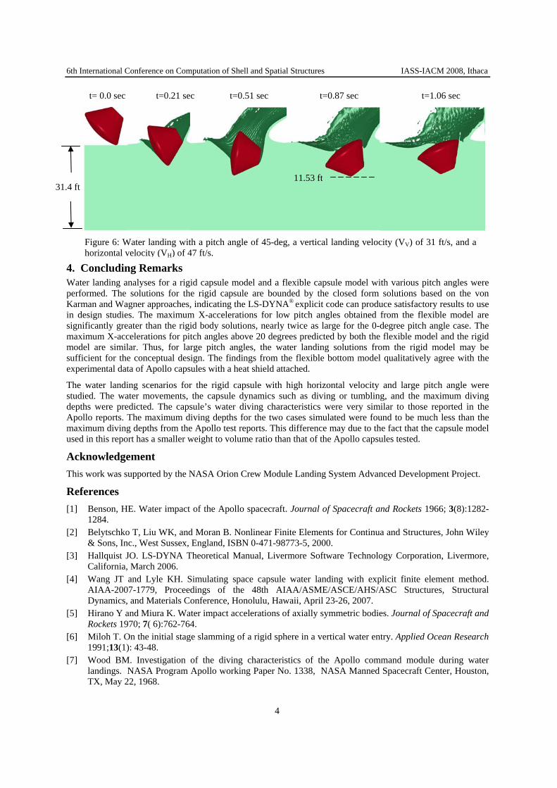
For the Region II landing scenario, the capsule impacted the water with a pitch angle of 40 degrees, a vertical landing velocity (VV) of 35 ft/s, and a horizontal velocity (VH) of 30 ft/s. Figure 5 shows the dynamic motions of the capsule and the water movement. The front half of the water block was removed to reveal the detailed dynamic motions of the capsule and the water. The buoyancy force for the capsule, due to the gravity induced pressure gradient in the water, was modeled in the analysis. For the Region III landing scenario, the capsule impacted the water with a pitch angle of 45 degrees, a vertical landing velocity (VV) of 31 ft/s, and a horizontal velocity (VH) of 47 ft/s. The capsule trips at its lower edge and rotates clockwise as shown in Figure 6, which may cause significant impact pressures on the conical sidewall and top deck. The maximum diving depths of the rigid capsule with the Regions II and III landing scenarios are 11.01 ft and 11.53 ft, respectively. These depths are less than those, around 18.0 ft, reported from the Apollo capsule tests for the same landing scenarios. The shallower diving depths predicted from the rigid capsule model may be due to the fact that its weight to volume ratio is about 60% of that of the Apollo capsules tested.

-20

0

20

40

60

80

0 10 20 30 40 50

Max

imum

Y-R

otat

iona

l Acc

eler

atio

n, ra

d/se

c2

Pitch Angle, deg

Flexible Model

Rigid Model

Figure 4: Maximum Y-rotational acceleration as a function of pitch angle.

Figure 3: Maximum X-acceleration as a function of pitch angle.

-35

-30

-25

-20

-15

-10

-5

0

-10 0 10 20 30 40 50

Max

imum

X-A

ccel

erat

ion,

g

Pitch Angle, deg

Rigid Model

von Karman Solution

Wagner SolutionFlexible Model

Figure 5: Water landing with a pitch angle of 40-deg, a vertical landing velocity (VV) of 35 ft/s, and a horizontal velocity (VH) of 30 ft/s.

21.4 ft 11.01ft

t= 0.0 sec t=0.24 sec t=0.52 sec t=0.80 sec t=1.20 sec


4

4. Concluding Remarks Water landing analyses for a rigid capsule model and a flexible capsule model with various pitch angles were performed. The solutions for the rigid capsule are bounded by the closed form solutions based on the von Karman and Wagner approaches, indicating the LS-DYNA® explicit code can produce satisfactory results to use in design studies. The maximum X-accelerations for low pitch angles obtained from the flexible model are significantly greater than the rigid body solutions, nearly twice as large for the 0-degree pitch angle case. The maximum X-accelerations for pitch angles above 20 degrees predicted by both the flexible model and the rigid model are similar. Thus, for large pitch angles, the water landing solutions from the rigid model may be sufficient for the conceptual design. The findings from the flexible bottom model qualitatively agree with the experimental data of Apollo capsules with a heat shield attached.

The water landing scenarios for the rigid capsule with high horizontal velocity and large pitch angle were studied. The water movements, the capsule dynamics such as diving or tumbling, and the maximum diving depths were predicted. The capsule’s water diving characteristics were very similar to those reported in the Apollo reports. The maximum diving depths for the two cases simulated were found to be much less than the maximum diving depths from the Apollo test reports. This difference may due to the fact that the capsule model used in this report has a smaller weight to volume ratio than that of the Apollo capsules tested.

Acknowledgement This work was supported by the NASA Orion Crew Module Landing System Advanced Development Project.

References [1] Benson, HE. Water impact of the Apollo spacecraft. Journal of Spacecraft and Rockets 1966; 3(8):1282-

1284. [2] Belytschko T, Liu WK, and Moran B. Nonlinear Finite Elements for Continua and Structures, John Wiley

& Sons, Inc., West Sussex, England, ISBN 0-471-98773-5, 2000. [3] Hallquist JO. LS-DYNA Theoretical Manual, Livermore Software Technology Corporation, Livermore,

California, March 2006. [4] Wang JT and Lyle KH. Simulating space capsule water landing with explicit finite element method.

AIAA-2007-1779, Proceedings of the 48th AIAA/ASME/ASCE/AHS/ASC Structures, Structural Dynamics, and Materials Conference, Honolulu, Hawaii, April 23-26, 2007.

[5] Hirano Y and Miura K. Water impact accelerations of axially symmetric bodies. Journal of Spacecraft and Rockets 1970; 7( 6):762-764.

[6] Miloh T. On the initial stage slamming of a rigid sphere in a vertical water entry. Applied Ocean Research 1991;13(1): 43-48.

[7] Wood BM. Investigation of the diving characteristics of the Apollo command module during water landings. NASA Program Apollo working Paper No. 1338, NASA Manned Spacecraft Center, Houston, TX, May 22, 1968.

Figure 6: Water landing with a pitch angle of 45-deg, a vertical landing velocity (VV) of 31 ft/s, and a horizontal velocity (VH) of 47 ft/s.

t= 0.0 sec t=0.21 sec t=0.51 sec t=0.87 sec t=1.06 sec

31.4 ft 11.53 ft




On a geometrically exact contact description for shells: from linear approximations for shells to high-order FEM Alexander KONYUKHOV, Karl SCHWEIZERHOF

University of Karlsruhe, Institute of Mechanics D-76128, Karlsruhe, Kaiserstrasse 12, Karlsruhe, Germany {Konyukhov, Schweizerhof}@ifm.uni-karlsruhe.de

Abstract Current computational models for shells allow effectively to describe the behavior of thin-walled structures

made of materials incorporating various non-linear constitutive relations independent of the order of approximation of shells. However, in combination with contact, new problems arise due to the remaining geometrical discontinuities of the normal vectors on element boundaries. This led to the development of smoothing techniques for contact interfaces based on covering the linear mesh with other surface approximations possessing the required smoothness on the element boundaries. The main difficulty is then a contact description including the correct kinematics and tangent matrices with regard to the new smooth surfaces. The covariant description developed during the recent years allows to enforce the exact kinematics point-wisely on contact surfaces with arbitrary approximation following then the exact geometry of the surfaces together with the formulation of tangent matrices in a covariant explicit form. Various examples starting with bi-linear and bi-quadratic solid-shells elements and finally with hierarchically constructed high order finite elements are chosen to show the efficiency of the proposed approach.

1. Introduction Modern computational models for shells cover many aspects in numerical modeling of real engineering

structures. Thus, the effectiveness of e.g. the solid-shell elements with different locking free formulations including EAS, ANS approaches, see e.g. for bilinear finite elements in Hauptmann et.al. [1], and for biquadrate FE in Hauptmann et.al. [2] has been verified for various cases of geometry and loading. Rank et.al. in [3] systematically applied the high order finite element technique in order to model shell structures with an exact geometry (via the, so-called, blending function method). In order to deal with arising discontinuity on element boundaries when the linear finite elements are used, in due course, in computational contact mechanics various smoothing techniques have been developed based on covering the linear mesh with other surface approximations possessing the required smoothness on the element boundaries, see the overview in Wriggers [4] and in Laursen [5]. In order to describe contact interactions between arbitrarily shaped bodies including various geometrical situations such as surface-to-surface, surface-to-curved line etc. a unified geometrical description fully based on the geometrical properties of those features, a, so-called, covariant approach has been developed recently, see Konyukhov and Schweizerhof [6], [7]. The approach is based on the description of all necessary parameters for contact in the specially defined coordinate system invoked by the corresponding closest point projection (CPP) procedure:

min),(),( 2121 →−= ξξρξξ srF (1)

where is vector of the slave contact point and is its projection onto the contact surface. The projection leads to a spatial curvilinear coordinate system defined by surface tangent vectors and the normal:

sr ),( 21 ξξρ

21

212211 n ; ;

ρρρρ

ξρρ

ξρρ

××

=∂∂

=∂∂

= for (2) nr 321321 ),(),,( ξξξρξξξ +=

1


One of the fundamental results achieved within the developing description is the solvability problem of the CPP procedure for surfaces of arbitrary geometry considered in Konyukhov and Schweizerhof [8]. Based on these results it is possible to construct the projection domains for arbitrary surfaces for which the projection exists and is unique. It has been shown that for arbitrary surfaces the CPP procedure should be generalized and should include projections not only onto surfaces, but also to edges and to points.

An extensive application of the differential geometry of surfaces is necessary then a) to formulate a weak form; b) to formulate various known methods to enforce contact conditions (penalty, augmented Lagrange multiplier, full Lagrange multiplier and Mortar methods); c) to consider linearization procedures in the form of covariant derivatives. Such a methodological procedure is then following the intrinsic surface geometry exactly and is thus independent of the following approximation of the contact surfaces.

2. Contact kinematics As natural measures of normal contact interaction representing the non-frictional case the third coordinate is taken, and the rate of the first two convective coordinates is taken as a measure of the tangential interaction representing the frictional case. A formulation in rate form allows then successfully to exploit the kinematical analogy for covariant derivatives as well as to formulate frictional forces with regard to the elasto-plastic analogy. Some further parameters for the isotropic frictional case are summarized in the Table 1:

3ξ21,ξξ &&

Deformation measures for normal direction 3ξ

for tangential traction 2,1 , =∆ iiξ

Rate of deformation for normal direction nv)v( s3 ⋅−=ξ&

for tangential direction 2,1, ,v)v( s =⋅−= jiρa iijjξ&

Constitutive equations for tangent traction vector R from a slave surface represented in metrics of the master surface

2,1, ,nR ss =+= jiρTN ii

normal traction 3ξε &NN −=

tangential traction (sticking) 3)( ξξε && stk

ki

jstk

kijijT

sti ThTa

dtdT

−Γ+−=

tangential traction (sliding) lk

kl

jij

T

sli

a

aN

dtdT

ξξ

ξµ

&&

&−=

where TN εε , are normal resp. tangential penalty parameters, are components of the metrics resp. the curvature tensor and are Christoffel symbols for the contact surface.

ki

ij ha ,kijΓ

Table 1: Summary of contact kinematics

The real tangential tractions are computed via the standard return-mapping scheme. The covariant formulation for the isotropic case can be generalized via the principle of maximum dissipation into coupled anisotropy including adhesion and friction, see Konyukhov and Schweizerhof [9], [10].

The weak form is obtained taking into account the pointwise equilibrium on the contact area. The contact integral is represented then as integral over the slave area as ss

(3) ∫∫ +=ss S

si

iS

sc dsTdsNW δξδξδ 3

The linearization of the integral (3) is fully taken in the metrics of the master surface and is expressed in explicit covariant form via the corresponding convective coordinates and force components, see in [6], [7].

2


3. Incorporation of a nonlinear approximation of the boundary It is shown within the covariant description; see [6], [7], [9], that all tangent matrices formulated in explicit

form contain a geometry approximation operator . This leads to a straightforward implementation of the derived algorithm with regards to any approximation of the geometry. In the case of application of high order FEM in combination with the blending function method as well as in the case of an iso-geometrical finite element approach the corresponding geometry approximation operator

is a non-linear operator with respect to the nodal (resp. knot) vector . In this case this operator should be additionally linearized as

),(A(x) 21 ξξρ sr−=

),(),A(x, 2121 ξξρξξ sr−= x

. (4) ),DA(0,...),DA(0,),A(0,),x,A(),( 2121212121 ξξξξξξξξδξξδδρ =++==− sr

Thus, in the case of a nonlinear approximation of the boundary all contact matrices will be computed following the pattern for linear approximation but with the corresponding linearized matrix , see [10]. ),DA(0, 21 ξξ

4. Numerical examples The simple deep-drawing problem in Fig. 1 is chosen to show the result of smoothing considering different order of the finite element approximation. The strip is modeled, first, with bi-linear solid shell elements. The solution though converging leads to a highly oscillatory behavior of the “control displacement-thickness strain” curve, Fig. 1 b). The application of bi-quadratic finite elements leads to almost perfect elimination of the oscillations.

a)

b) c)

Figure 2: Deep drawing of a strip. a) – finite element model and thickness strain-control displacement curve for: b) bi-linear finite elements, c) bi-quadratic finite elements.

Another numerical example is aimed to show an application of the contact description to high order finite elements. The classical Hertz problem is modeled first with a completely linear finite element mesh, see Fig. 2 a). Afterwards, a few elements on the contact boundary are modified into, so-called, Contact Layer finite elements, Fig. 2 b). These elements are constructed as anisotropically p-refined elements with an exact representation of the boundary via the blending function method, see details in [10]. A good correlation with the Hertz solution is found even in cases where the contact zone lays inside the single finite element, Fig. 2c).

3


a) b)

c)

Figure 2: FE model for the Hertz problem. a) – initial bi-linear mesh; b) six elements are modified into Contact Layer finite elements; c) contact pressure vs. contact radius, contact zone is inside a single element.

References [1] Hauptmann R., Schweizerhof K., Doll S. Extension of the solid-shell concept for application to large

elastic and large elastoplastic deformations. International Journal for Numerical Methods in Engineering 2000; 49:1121-1141.

[2] Hauptmann, R., Doll S., Harnau M., Schweizerhof K. “Solid-Shell” Elements with Linear and Quadratic Shape Functions at Large Deformations with Nearly Incompressible Materials. Computers & Structures 2001; 79:1671-1685.

[3] Rank E., Duester A., Nuebel V., Preusch K., Bruhns O.T. High order finite elements for shells. Computer Methods in Applied Mechanics and Engineering 2005; 194:2494-2512.

[4] Wriggers P. Computational Contact Mechanics. (2nd edn). Springer, 2006. [5] Laursen T.A. Computational Contact and Impact Mechanics. Springer, 2002. [6] Konyukhov A., Schweizerhof K. Contact formulation via a velocity description allowing efficiency

improvements in frictionless contact analysis. Computational Mechanics 2004; 33: 165-173. [7] Konyukhov A., Schweizerhof K. Covariant description for frictional contact problems. Computational

Mechanics 2005; 35: 190-213. [8] Konyukhov A., Schweizerhof K. On the solvability of closest point projection procedures in contact

analysis: Analysis and solution strategy for surfaces of arbitrary geometry. Computer Methods in Applied Mechanics and Engineering 2008: doi:10.1016/j.cma.2008.02.09.

[9] Konyukhov A., Schweizerhof K. Covariant description of contact interfaces considering anisotropy for adhesion and friction. Computer Methods in Applied Mechanics and Engineering 2006; Part 1 – 196(1-3):103—117; Part 2 – 196(1-3) 289-303.

[10] Konyukhov A., Schweizerhof K. Incorporation of contact for high order finite elements in covariant form. Computer Methods in Applied Mechanics and Engineering 2008 (accepted for publication).

4

geometry and mechanics - core.ac.uk vascular blood ﬂow with the purpose of designing predictive...

Documents