geometric phase in quantum theory - theor.physics.muni.cz

Faculty of ScienceMASARYK UNIVERSITY

Diploma Thesis

Geometric phase in quantumtheory

Brno, 2006 Ales Navrat

I declare that I have worked out the diploma thesis indepen-dently and I have mentioned all literature sources I used.

Brno, January 2006

I would like to thank Tomas Tyc, M.S., PhD for leading of mydiploma thesis, the provided literature, and the time he devotedto me.

Contents

1 Introduction 11.1 A guide through this work . . . . . . . . . . . . . . . . . . . . . . . 11.2 Motivational example . . . . . . . . . . . . . . . . . . . . . . . . . . 2

2 Geometric phases in physics 62.1 Berry phase . . . . . . . . . . . . . . . . . . . . . . . . . . . . . . . 72.2 Berry phase in the degenerate case . . . . . . . . . . . . . . . . . . 102.3 Aharonov-Anandan phase . . . . . . . . . . . . . . . . . . . . . . . 11

3 Experiments and applications 153.1 Photons in an optical fibre . . . . . . . . . . . . . . . . . . . . . . . 163.2 Geometric phase and Aharonov-Bohm effect . . . . . . . . . . . . . 193.3 Three-level systems in interferometery . . . . . . . . . . . . . . . . 213.4 Applications . . . . . . . . . . . . . . . . . . . . . . . . . . . . . . . 24

4 Geometrical interpretation 264.1 Holonomy interpretations of the geometric phase . . . . . . . . . . . 264.2 Degenerate case . . . . . . . . . . . . . . . . . . . . . . . . . . . . . 314.3 Structure of the parameter space . . . . . . . . . . . . . . . . . . . 334.4 More on the Berry’s phase . . . . . . . . . . . . . . . . . . . . . . . 354.5 The non-adiabatic case . . . . . . . . . . . . . . . . . . . . . . . . . 36

5 Simple examples 405.1 The adiabatic nondegenerate case . . . . . . . . . . . . . . . . . . . 405.2 The adiabatic degenerate case . . . . . . . . . . . . . . . . . . . . . 415.3 The nonadiabatic case . . . . . . . . . . . . . . . . . . . . . . . . . 42

6 Conclusion 44

iii

Chapter 1

Introduction

1.1 A guide through this work

Although the concept of geometric phase came originally from the quantumtheory, the similar phenomenon can be found also in the classical physics.In the beginning, I give an example of such the phenomenon, namely theone, arising from the motion of the globe. It should serve for having later abetter insight into the original problem in quantum physics and, especially,one should see how it is closely related to the geometry.

Two different approaches to geometric phases are defined in the secondchapter. The original Berry phase for the cyclic adiabatic evolutions and theAharonov-Anandan phase for the general cyclic evolutions of the physicalsystems. The basic properties and connections between are briefly sketchedand the formalism is illustrated on the well-known example, namely theoccurance of an electron in a rotating magnetic field is discussed.

Some experiments manifesting the presence of a geometric phase factor(and important to my mind) are listed in the third chapter. Namely, thecase of photons in a helically coiled optical fibre, the geometric phase inthe Aharonov-Bohm effect and the geometric phase of three-level systems ininterferometry is analyzed. To conclude this chapter, the (possible) applica-tions are briefly discussed.

The rich mathematical tool is applied in the fifth chapter and the geomet-ric phase is interpreted as arising from the holonomy in some bundle. Thisgeometrical interpretation brings a new point of view. Especially the meaningof the adjective ”geometrical” is clear, but moreover, the other properties of

1

CHAPTER 1. INTRODUCTION 2

the geometric phase are easy to be shown. The classification theorem is alsobriefly discussed. The adiabatic case is discussed in detail to get calculationuseful formulae.

The last chapter is devoted to simple examples of the formalism intro-duced in the previous chapter.

1.2 Motivational example

Geometrical phases arise due to a phenomenon which can be describedroughly as ”a global change without any local change”. For better under-standing, the following example of the motion of the globe is especially illus-trative.

We consider that the globe rotates with a constant angular velocity ωbut that the direction of the vector of angular velocity ω(t) varies in time.Moreover we assume that this change of the direction is slow with respectto ω. To be more precise, assume that the change is such that the vector ofangular velocity rotates slowly with an angular velocity Ω around the z axisof a coordinate system, which is fixed in the outer space and which has theorigin in the center of the globe. The vector ω(t) remains in the xy-plane.Then we can write:

ω(t) = ω · (cos Ωt, sin Ωt, 0)T .

We now choose a moving coordinate system (x, y, z), in which the directionof ω(t) is fixed in x-direction and the axes y and z remain ”in the samedirection”, i.e. parallel, with respect to the globe. Rigorously, they areparallelly transported with respect to the globe, i.e. the infinitesimal changeof the unit vectors y and z in every point is perpendicular to the globe. Thenthe equations of motion dr

dt= ω × r have a simple form

d

dt

xyz

=

0 Ω 0

−Ω 0 −ω0 ω 0

xyz

.

The matrix is obviously singular and has one real eigenvalue 0 with a corre-sponding eigenvector given by c(t) · (1, 0, Ω

ω)T . This means nothing else but

that in the so called adiabatic limit,i.e. Ωω→ 0, the point (1, 0, 0)T , i.e. the

north pole, is a stationary point. Thus we have proved that if the variation


of direction of angular velocity is small enough, the position of the rotationaxis with respect to the body is fixed, which is referred to as an adiabatictheorem for the rigid body motion.

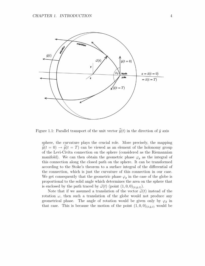
Let us now assume that the vector of angular velocity is slowly changing,for example in such a way as it is depicted in the picture 1.1. It meansthat in the beginning (t = 0) we have (x, y, z) = (x, y, z). Then the vectorω(t) moves along a meridian then along the equator and then along anothermeridian until it comes back to the starting point (t = T ). According tothe adiabatic theorem, the rotation axis traces the same closed path. Itmeans that after the circuit, the globe will be in the same state x = x upto a rotation in the yz-plane. It is now easy to compute the angle of thisrotation.

One could guess that the angle equals∫ T0ω(t)dt at first glance. But a

bit properer treatment shows that it is not the truth. It holds only in thecoordinate system (x, y, z). The angle of the rotation with respect to this

system after the time T is really ϕd =∫ T0ω(t)dt = ωT . But the system

(x, y, z) in the time t = T does not coincide with the system (x, y, z), whichis fixed in the outer space (in t = 0 they coincide). As the angular velocity is

moving on the sphere, the unit vector x is still normal to the sphere and theunit vectors y, z are still the tangent vectors and they remain parallel (doesnot rotate around the x axis). In the words of differential geometry: they areparallelly transported along the closed path. Because of the curvature of thesphere (that represents the globe), there will be a nonzero angle ϕg betweenthe axis y (or z equivalently) in t = 0 and t = T (or equivalently between

the vectors y(t = 0) and y(t = T )). One can see this in figure 1.1. The resultis: Although the axis of rotation comes back to the starting point after thetime T , the globe is not in the same position. The final position differs fromthe original about the angle ϕ in the yz-plane which can be computed as thesum of two angles ϕ = ϕd + ϕg. I will call these angles phases in analogywith the quantum case. ”Phase” is used meaning just ”angle” for whateverpossible argument of sin(·) or cos(·) or exp(·). The first angle (phase) ϕdarise due to the angular velocity ω and the second angle (phase) ϕg arise dueto the parallel transport on the sphere. Therefore the former can be called”dynamical phase” and the latter ”geometric phase”.

In the following, I will focus on the latter. The adjective ”geometric”is apposite, because it is the geometry of the space on which the motionis fixed that determines the factor ϕg. Generally, as in our case of the


Figure 1.1: Parallel transport of the unit vector y(t) in the direction of y axis

sphere, the curvature plays the crucial role. More precisely, the mappingy(t = 0) → y(t = T ) can be viewed as an element of the holonomy groupof the Levi-Civita connection on the sphere (considered as the Riemannianmanifold). We can then obtain the geometric phase ϕg as the integral ofthis connection along the closed path on the sphere. It can be transformedaccording to the Stoke’s theorem to a surface integral of the differential ofthe connection, which is just the curvature of this connection in our case.We get consequently that the geometric phase ϕg in the case of the globe isproportional to the solid angle which determines the area on the sphere thatis enclosed by the path traced by ω(t) (point (1, 0, 0)(x,y,z)).

Note that if we assumed a translation of the vector ω(t) instead of therotation ω, then such a translation of the globe would not produce anygeometrical phase. The angle of rotation would be given only by ϕd inthat case. This is because the motion of the point (1, 0, 0)(x,y,z) would be


fixed to the flat subspace. This is really the curvature of the sphere which isresponsible for the geometric phase.

I would like to mention that the rotation of Foucault pendulum can also beexplained by such a holonomy. In this example, the vector which determinesthe direction of oscillating and which is tangent to the sphere (Earth) isparallelly transported.

In these classical examples, ”no local change” means that the tangentvector remains locally parallel during the whole evolution and ”the globalchange” is the angle ϕg between the starting and the final vector. Thiscan be explained by the holonomy of the natural connection on the tangentbundle of sphere.

Nearly the same situation occurs in quantum physics. Here a systempicks up a geometric phase after a cyclic evolution. This is again given bythe holonomy of a connection in a certain bundle.

Chapter 2

Geometric phases in physics

In this chapter, I introduce two different approaches to the so called geometricphase. The first part is dedicated the original derivation of Berry [2], whichpoints out that a system which evolves cyclically under an adiabatic conditionpicks up an additional phase factor which turns out to be geometrical innature. The Berry’s concept is then shown on an example. A generalizationto the degenerate case, done by Wilczek and Zee [5], is treated in the secondpart. Because of the special adiabatic condition, Aharonov and Anandan [3]tried to remove this condition and to generalize the occurance of the phaseto evolutions that have to fulfill only the cyclic condition. This is introducedin the second part. Each part contains a general derivation of the ideas, I donot specialize in the geometrical meaning.

Before starting with the Berry phase, I should mention that, in fact,the first geometric phase was introduced by Pancharatnam already in 1956[1]. In this article about the interference of polarized light, he defines aphase difference of two nonorthogonal polarization states. According to[1], two states are said to be ”in phase” if the intensity of the superposedstate is maximal. The phase difference is then the phase shift which hasto be applied to one of the states in order to be in this relation with thesecond. Further, Pancharatnam points out that this phase has a geometricalmeaning, which arises from the fact that the relation ”to be in phase” is nottransitive. Namely, let us consider three mutually nonorthogonal states ofpolarization, which are represented by three points A,B,C on the Poincaresphere (Poincare sphere is a well-known representation for the manifold ofpure polarization states of a plane electromagnetic wave [1]). If the statesare arranged such that A and B are ”in phase” and B and C are ”in phase”,

6

CHAPTER 2. GEOMETRIC PHASES IN PHYSICS 7

then, in general, the states corresponding to the points A and C are not”‘in phase”. Pancharatnam also calculated the extend to which these lasttwo states are ”out of phase” and showed that this ”phase difference” equalsone half the solid angle on the Poincare sphere determined by the sphericaltriangle ABC obtained by joining the vertices A,B and C by great circle arcs(geodesic arcs) on the sphere.

The results of Pancharatnam has been later interpreted in the contextof all two-level quantum systems, for which the space of pure state densitymatrices is again the sphere S2. The representation is determined by theobvious identification SU(2)/U(1) = SO(3)/SO(2) = S2. For the three-levelsystems, there exists a generalization of the Poincare sphere representation[4]. In that case, the coset space SU(3)/U(2) is represented by a simplyconnected region in S7.

2.1 Berry phase

In 1984, Berry published a paper [2] in which he considers cyclic evolutionsof systems under special, so called adiabatic, conditions. He finds that acyclic evolution of a wave function yields the original state plus a phaseshift, and this phase shift is a sum of a dynamical phase and a geometric (ortopological, or Berry) phase shift. Berry points out the geometrical characterof this phase is not negligible. The phase is gauge invariant and therefore cannot be gauged out as was earlier supposed. Many articles has been alreadywritten to this subject and, consequently, the so-called Berry phase is nowwell established, both theoretically as experimentally.

The original point of view of Berry is ”dynamical”. By this I mean thathe starts with a Hamiltonian H that describes the quantum system in ques-tion. Further he considers that the Hamiltonian depends on a multidimen-sional real parameter x which parametrizes the environment of the system.Then the time evolution of the system is determined by the time dependentSchrodinger equation

H(x(t))|ψ(t)〉 = i∂

∂t|ψ(t)〉

We can choose a basis of eigenstates |n(x(t))〉 corresponding to the energiesEn, i.e. such that

H(x(t))|n(x(t))〉 = En(x(t))|n(x(t))〉


is fulfilled. In the moment, we assume that the energy spectrum of H isdiscrete, that the eigenvalues are not degenerated and that no level crossingoccurs during the evolution. Moreover, suppose that the environment andtherefore x(t) is adiabatically varied. It means that the changes are slow intime with respect to the characteristic time scale of the system (given by thePlanck’s constant divided by the energy difference of two neighboring energylevels). Then the adiabatic theorem holds and thus, when the system startsin the n-th energy eigenstate, i.e. |ψ(0)〉 = |n(x(0))〉, the system will beover the whole evolution at the n-th energy level. But, in general, the statevector gains a phase factor, i.e. |ψ(t)〉 = eiφn |n(x(t))〉. At first sight, onewould guess that the phase factor equals θn(t) = −1

∫ t0En(τ)dτ but the point

is that the Schrodinger equation allows an additional phase factor γn(t), i.e.φn = θn+γn. The former is now called the dynamical phase and the latter thegeometric phase (notice the similarity to the motivational example). Puttingthis to the Schrodinger equation we get the following condition for γn:

∂

∂t|n(x)〉 + i

d

dtγn(t)|n(x)〉 = 0

or equivalently in a nice form

d

dtγn(t) = i〈n(x)| ∂

∂t|n(x)〉 = i〈n|∇|n〉dx

dt.

Now, when we are given a cyclic evolution, described by a closed curveC : t → x(t) with x(T ) = x(0), then the Berry phase for such an evolutionis given by the following simple expression

γn(C) = i

∮C

〈n(x)|∇|n(x)〉dx.

From this, one can easily see that the Berry phase depends on the geometryof the parameter space (and on the loop C therein). That is why Berrycalled this phase factor ”geometric phase”. Now, geometric phase is used asa universal notion for various generalizations of the original Berry’s phase.

Let me briefly show how the Berry phase emerges in the concrete example.Namely, in the famous and important example when a spin- 1

2particle occurs

in a magnetic field. I will proceed along the lines of [18]. Consider that

the spin- 12

particle is moving in an external magnetic field B which rotatesadiabatically (slowly) under an angle θ around z-axis as it is depicted in 2.1.Then the magnetic field is given by


Figure 2.1:

B(t) = B0

sin θ cos(ωt)

sin θ sin(ωt)cos θ

where ω is the angular frequency of the rotation and B0 = | B(t)|. Whenthe field rotates slowly enough and the expected value of the spin was in thedirection of field, then the spin of the particle will follow the direction ofthe field and an eigenstate of the Hamiltonian H(0) stays for all times t aneigenstate of H(t). The interaction Hamiltonian for this system in the rest

frame is given by H(t) = µ B · σ, where σ are Pauli matrices and µ = 12em

is the magnetic dipole moment connected with the spin. When we now usethe explicit form of B we get two normalized eigenstates of H(t)

|n+(t)〉 =

(cos θ

2

eiωt sin θ2

), |n−(t)〉 =

( − sin θ2

eiωt cos θ2

)

with the corresponding energy eigenvalues E± = ±µB0. A calculation of∇|n±(t)〉 in the spherical coordinates B0, θ, φ(t) = ωt leads to rather simpleexpressions

〈n+|∇|n+〉 = isin2( θ

2)

B0 sin θ, 〈n−|∇|n−〉 = i

cos2( θ2)

B0 sin θ


The curve C in parameter space (which is now sphere) is given by C : B0 =const., θ = const., φ ∈ [0, 2π]. Thus the Berry phase in this example equals

γ±(C) = i

∮C

〈n±|∇|n±〉B0 sin θdφ = −π(1 ∓ cos θ).

This is nothing else but the half of the solid angle enclosed by the path Cand so we get the final expression

γ±(C) = ∓1

2Ω(C).

We see that whereas the dynamical phase (which is now given by ±µB0T )

depends on the period T of the rotation, the geometrical phase depends onlyon the special geometry of the problem.

2.2 Berry phase in the degenerate case

A generalization for the degenerate Hamiltonians was done by Wilczekand Zee [5]. From the comments above, one can deduce that the termi〈n(x)|∇|n(x)〉 plays a role of a gauge potential in a U(1) gauge field. Thisalso shows that the Berry phase is a gauge invariant object and it is not pos-sible to remove it by a certain choice of the basis states of the Hamiltonian.The direct generalization leads to non-abelian gauge field U(n). Supposethat we are given a family of Hamiltonians H(x) depending continuously onparameters x that has a n-times degenerate level for each value of x. Bya simple renormalization of the energies, we can suppose that these levelsare at E = 0. The degenerate levels are mapped back onto themselves byadiabatic development and this mapping is nontrivial in general. To showthis, choose an arbitrary smooth set of bases |na(t)〉 for the various spaces ofdegenerate levels, so that

H(x(t))|na(t)〉 = 0

Let the solutions |ma(t)〉 of the Schrodinger equation with the initial condi-tion |ma(0)〉 = |na(0)〉 are given by

|ma(t)〉 = Uab(t)|nb(t)〉.


Writing this equation, we have assumed the adiabatic evolution and our taskis to determine U(t). We demand that the |ma(t)〉 remains normalized andthis leads to the equation

(U−1U)ab = −〈na|nb〉 ≡ Aab

and this anti-Hermitian matrix Aab plays the role of a gauge potential. Thenthe desired mapping given by a closed path in the parameter space has theform

U = Pe∮Aµdxµ

where P is the path ordering operator and xµ are coordinates in the param-eter space. This is known as the Wilson loop.

2.3 Aharonov-Anandan phase

In 1987, Aharonov and Anandan [3] considered cyclic evolutions that arenot restricted by an adiabatic condition and purposed an generalization ofBerry’s phase. This generalization is very important, because the adiabaticcondition is never exactly fulfilled for real evolutions. In the adiabatic ap-proximation, Aharonov and Anandan phase then tends to the Berry phase ifthe parameters are chosen accordingly.

The appearance of Aharonov and Anandan phase (and other phases andrelated phenomena) can be explained in terms of quantum mechanics. Thecrucial role plays the fact that in quantum physics the physical state of asystem is only determined up to a phase. The physical states are thereforein a bijective correspondence with points in the projective Hilbert space, i.e.with the pure-state density matrices. But usually, it is better to computein Hilbert space and then pass to the projective space. This is due to thefact that the geometry of Hilbert space (and the computation therein) issimpler. The interplay between the Hilbert space and its projective space isresponsible for the phenomena that I discuss here.

According to Aharonov and Anandan, I show the existence of a phaseassociated with cyclic evolution, which is universal in the sense that it isthe same for the infinite number of possible motions along the curves inthe Hilbert space H which project to a given closed curve in the projectiveHilbert space P of rays of H. Moreover, it is the same for all the possibleHamiltonians H(t) which propagate the state along these curves.


The question is, what phase factor eiΦ (which can have observable con-sequences) that the initial and the final state vector of a cyclic evolutionmay be related by. Suppose that the normalized state |ψ(t)〉 ∈ H evolvesaccording to the Schrodinger equation

H(t)|ψ(t)〉 = i∂

∂t|ψ(t)〉,

such that the evolution is cyclic, i.e. |ψ(T )〉 = eiΦ|ψ(0)〉. Let Π : H → P bethe projection map defined by

Π(|ψ〉) = |ψ′〉 : |ψ′〉 = c|ψ〉, c is a complex number.

Then |ψ(t)〉 defines a curve C : [0, T ] → H with C ≡ Π(C) being a closedcurve in P. Conversely given any such curve C, we can define a Hamil-tonian function H(t) so that the Schrodinger equation is satisfied for thecorresponding normalized |ψ(t)〉. Now define

|ψ(t)〉 = e−if(t)|ψ(t)〉

such that f(T )−f(0) = Φ. Then |ψ(t)〉 is exactly cyclic, i.e. |ψ(T )〉 = |ψ(0)〉,and from Schrodinger equation,

−dfdt

=1

〈ψ(t)|H|ψ(t)〉 − 〈ψ(t)|i d

dt|ψ(t)〉.

Hence, if we remove the dynamical part from the phase Φ by defining

β ≡ Φ +1

∫ T

0

〈ψ(t)|H|ψ(t)〉dt,

it follows from the above equation that

β =

∫ T

0

〈ψ|i ddt|ψ〉dt.

This is the final expression for the Aharonov-Anandan phase. Clearly, thesame |ψ(t)〉 can be chosen for every curve C for which Π(C) = C, byappropriate choice of f(t). Hence such β, as defined above, is independentof the total phase Φ and Hamiltonian H for a given closed curve C. Indeed,from the last expression, β is independent of the parameter t of C, and is


uniquely defined up to 2πn (n = integer). Hence eiβ is a geometric propertyof the unparameterized image of C in P only and therefore can be viewedas the second (or third) example of a geometric phase. Moreover, it is auniversal phase in a certain sense (as we will see later).

Now, I will prove along the lines in [3] that in the adiabatic approx-imation, the phase found by Aharonov and Anandan tends to the phasefound by Berry. Consider therefore a slowly varying Hamiltonian H(t), withH(t)|n(t)〉 = En(t)|n(t)〉, for a complete set |n(t)〉. If we set

|ψ(t)〉 =∑n

an(t)e− i

∫Endt|n(t)〉,

then by using the Schrodinger equation and by differentiating the eigenvectorequation, we obtain

am = −am〈m|m〉 −∑n =m

an〈m|H|n〉En −Em

ei

∫(Em−En)dt,

where the dot denotes time derivative. In the adiabatic limit, we can furthersuppose that ∑

m=n

∣∣∣∣∣ 〈m|H|n〉(En − Em)2

∣∣∣∣∣ 1

holds and that the system starts in an eigenstate, i.e. an(0) = δmn. Then thelast term in the above expression of am is negligible and the system wouldtherefore continue as an eigenstate of H(t). In this approximation, we get

am(t) = e−∫ 〈m|m〉dtam(0).

Thus for a cyclic adiabatic evolution, this yields the phase i∫ T0〈m|m〉dt,

which is independent of the chosen |m(t)〉 and which is the phase found byBerry.

Berry regarded this phase as a consequence of geometrical properties ofthe parameter space of which H is a function. But this phase is the same asAharonov-Anandan phase β, when we approximate |ψ(t)〉 by |m(t)〉 and β,as defined, does not depend on any approximation and the expression β =∫ T0〈ψ|i d

dt|ψ〉dt is exactly valid. Moreover, |ψ(t)〉 need not be an eigenstate

of H(t), unlike in the adiabatic case of Berry. It is neither necessary norsufficient to go around a closed curve in parameter space in order to have a


cyclic evolution, with the associated geometric phase β. For these reasons,β is regarded as a geometric phase associated with a closed curve in theprojective Hilbert space and not the parameter space, even in the special caseconsidered by Berry. But given a cyclic evolution, a Hamiltonian H(t) whichgenerates this evolution can be found so that the adiabatic approximationis valid. Then β can be computed with the use of the expression given byBerry in terms of the eigenstates of this Hamiltonian.

Chapter 3

Experiments and applications

It seems to be impossible to measure the phase change |ψ〉 → eiϕ|ψ〉 at firstsight, because the normalized vectors |ψ〉 and eiϕ|ψ〉 represent the same stateof a physical system and hence the results of any measurement performedon them are the same. But, similarly to the wave optics, we can make somekind of an interference measurement. It means that some part of the physicalsystem in question can serve as a reference phase. The other part on whichthe phase shift is performed is then recombined with the first one to form aninterference pattern. This pattern is obviously different for different valuesof the phase shift ϕ.

The second task is to separate somehow the geometric phase from thistotal phase ϕ. Many of such experiments which measure the geometricphase shift have been already proposed and done. The Berry’s phase can bedemonstrated in experiments with photons by variation of the propagationdirection. It is the case of the coiled optical fibre [6] or the Mach-Zehnderinterferometer [7] for example. Other experiments with photons use variationof polarization to show up the Pancharatnam phase.

Another class of experiments are the experiments with neutrons. Neu-trons are fermions which are not sensitive to any electric field and hencethey are easy to handle. There are two groups of experiments with neutronsacquiring a geometric phase: neutron polarimeters and neutron interferome-ters. To the former, the experiment of Bitter and Dubbers belongs [8], wherethe effect of the Berry phase was first shown for fermions. To the latter, theexperiment of Hasegawa, Zawisky, Rauch and Ioffe [9] belongs for example.Other relevant experiments are these of nuclear magnetic resonance, nuclearquadrupole resonance or atom interferometer.

15

CHAPTER 3. EXPERIMENTS AND APPLICATIONS 16

3.1 Photons in an optical fibre

This was the first experiment to confirm the prediction of Berry. It waspurposed by R.Y. Chiao and Y.S. Wu [10] in 1986 and this year yet realizedby A. Tomita and R.Y. Chiao [6]. The photon’s spin vector, which pointseither along the direction in which it is travelling or in the opposite direction,can be easily turned by changing the direction of travel. In [10] and [6], it isdone with a coiled optical fibre. Let me introduce this experiment.

We assume that the light propagates inside the fibre in a single mode andits path is parametrized by the optical path length τ . Adiabatic conditionis the conservation of the helicity which says, in other words, that at eachpoint τ , the photon’s spin state |k(τ), σ〉 satisfies

s · k(τ)|k(τ), σ〉 = σ|k(τ), σ〉,

where k(τ) is the direction of propagation of the photon at τ and σ = ±1is its helicity quantum number. Formally, it is identical to the problemconsidered in the previous chapter for a spin s in an adiabatically changingmagnetic field B(t), gs · B(t)| B(t), ms〉 = E| B(t), ms〉, where g is relatedto the gyromagnetic ratio and ms is the component of the spin along thedirection of B(t). Now we extend the results from this case to the case ofphoton.

Suppose that the fibre is wounded in such a way that the vector k tracesout a closed curve, e.g. it is hellicaly shaped. In this case, we can use thederivation of Berry to determine the geometrical phase gained during thepath through the fibre. Now, the parameter space is the momentum spacek and the adiabatic invariant property is the helicity. Berry’s formula forthe photon is very similar to that for electrons. It only differs in a factor 1

2

which is a consequence of the difference of spins of photons and electrons.

γσ = −σΩ(C).

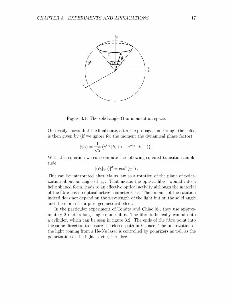
The solid angle Ω(C) is determined by the curve C that the k-vector tracesout in momentum space (figure 3.1). Now, let us consider a linearly polarizedlight which is a superposition of the helicity eigenstates

|ψi〉 =1√2(|k,+〉 + |k,−〉).


Figure 3.1: The solid angle Ω in momentum space.

One easily shows that the final state, after the propagation through the helix,is then given by (if we ignore for the moment the dynamical phase factor)

|ψf〉 =1√2

(eiγ+ |k,+〉 + e−iγ+ |k,−〉) .

With this equation we can compute the following squared transition ampli-tude

|〈ψi|ψf〉|2 = cos2 (γ+) .

This can be interpreted after Malus law as a rotation of the plane of polar-ization about an angle of γ+. That means the optical fibre, wound into ahelix shaped form, leads to an effective optical activity although the materialof the fibre has no optical active characteristics. The amount of the rotationindeed does not depend on the wavelength of the light but on the solid angleand therefore it is a pure geometrical effect.

In the particular experiment of Tomita and Chiao [6], they use approx-imately 2 meters long single-mode fibre. The fibre is helically wound ontoa cylinder, which can be seen in figure 3.2. The ends of the fibre point intothe same direction to ensure the closed path in k-space. The polarization ofthe light coming from a He-Ne laser is controlled by polarizers as well as thepolarization of the light leaving the fibre.


Figure 3.2: Experimental setup for measuring of the Berry’s phase in a helicaloptical fibre [6]

The experiment consists of two major parts. The first one is to use a fibrewitch is wound with a constant pitch angle θ. The Berry formula reads as

γσ(C) = −2πσ(1 − cos θ) = −2πσ(1 − p

s),

where s is the length of the fibre and p is the length of the cylinder. Thisequation was experimentally verified.

For the second part of the experiment, they used nonuniform woundhelical fibres, i.e. with the pitch angle θ dependent on a parameter τ . Thenthe solid angle of the closed curve C, traced out in momentum space, is givenby

Ω(C) =

∫ 2π

0

(1 − cos θ(τ)) dτ

and the Berry phase is γσ = −σΩ(C), which is again related to an opticalrotation which is measured. The measurements then verify these theoreticalpredictions.

Note that these optical effects could be explained in principle entirelyclassically in terms of Maxwell equations with the appropriate boundaryconditions. When the mutually orthogonal triad of vectors k, E and B willadiabatically propagate by parallel transport inside a wound fibre, it wouldlead to the above results. The problem is in that the classical theory fails forlow photon number, whereas the quantum theory still holds. Fundamentally,it is the the Bose nature of the photon which allows the appearance of these


optical manifestations of Berry phase on a classical level. These effects canbe therefore considered as topological features of classical Maxwell theorywhich arise in quantum mechanics, but survive the correspondence-principlelimit ( → 0) into the classical level.

3.2 Geometric phase and Aharonov-Bohm ef-

fect

In 1959, Y. Aharonov and D. Bohm demonstrated that the vector potentialhas more physical significance that had been previously thought [11]. Theysend two beams of electrons past a long tightly wound solenoid along bothsides (as in 3.3 depicted). It is well-known that the magnetic field of the

Figure 3.3: Measurement of the Aharonov-Bohm effect.

solenoid is very simple: it is uniform inside (and parallel to) the solenoid,and zero outside. Although the electrons occur only in the region whereB = 0, the change of interference pattern, observed when the beams arerecombined, manifests a phase difference of electrons. This phase differencearise due to the key fact that the vector potential A is nonzero outside thesolenoid.

When we choose a Coulomb gauge (i.e. ∇ · A = 0), the vector poten-tial outside the solenoid equals A = Φ

2πrφ, where Φ is the magnetic flux,

and r and φ (the azimuthal unit vector) are defined by setting the axis of


the solenoid as the axis of a cylindrical coordinate system (see figure 3.3).Aharonov and Bohm realized that the presence of the nonzero vector poten-tial fundamentally changed the behavior of the wave function. Space, for thewave function, is no longer simply connected and the integrals

∮A · dr are

path dependent. It is precisely the difference of such integrals between thetwo different paths around the solenoid that give rise to the Aharonov-Bohmeffect observed as a shift of the interference fringes.

Now, following [2], I show how this effect may be seen in terms of ageometric phase. The splitting and recombination of the beam of electronscan be viewed in such a way that the electrons goes backwards in time alongone path and returns along the other path to its original state at the sametime. It defines a circuit C around the solenoid. Let the physical (quantal)system, described by |n(R)〉, consist of an electron (or electrons), with acharge e, which is in a box that is centered in R and lies outside the solenoid.In the case of A = 0, the Hamiltonian for an electron depends on the positionof electron r and has a form of H(p, r−R). The corresponding wavefunctionsare ψn(r − R) with energies En independent of R. Now, when A = 0, thestates |n(R)〉 satisfy the eigenequation

H (p− eA(r), r − R) |n(R)〉 = En|n(R)〉.

One can verify that the exact solutions (in the coordinate representation) ofthis equation are obtained by multiplying ψn by an appropriate phase factoras follows:

〈r|n(R)〉 = eie

∫ rR A(r′)·dr′ψn(r −R).

Since the solenoid is not inside the box, the integral in this equation isindependent of the path from R to r. When we transport the system (box)round the circuit C, the system |n(R)〉 acquires a geometric phase factor.This factor can be calculated using the Berry’s formula from previous chapterand using

〈n(R)|∇Rn(R)〉 =∫ ∫ ∫

d3rψn(r − R)(− ie

A(R)ψn(r − R) + ∇Rψn(r − R)

)= − ie

A(R),

where the simplification is a consequence of the normalization of the wave-functions ψn. And finally, the Berry phase is given by

γn(C) =e

∮C

A(R) · dR =eΦ

.


The final line follows from the Stokes theorem. This result agrees with thatobtained in [11]. It is independent of n and also of C if this winds once andonly once round the solenoid. It is also obvious that C can be taken suchthat R is two-dimensional.

It means that the parameter space of the HamiltonianH is in fact R2. Butthis space is locally flat against the previous example, where the parameterspace was a sphere S2, which is obviously curved. One can not in any caseuse the Berry’s solid angle formula and it seems so that the geometric phaseshould be zero, although it is not the truth as we have computed. This”mystery” is the same as the ”mystery” of the Aharonov-Bohm effect-theelectron occurs in a field with B = 0 but nevertheless, it gains a phase factor.The core of this ”mystery” is in that the Hamiltonian has a singular point inr = 0. Thus the parameter space is R

2 \ 0 which is not simply connectedand the path integrals

∮A(R)·dR occuring in the expression of the geometric

phase are nonzero for the paths which enclose the singularity and hence thegeometric phase is nonzero. There is no problem to consider R ∈ R3. In thiscase, the singularity becomes a singular line l (representing the solenoid) andthus the parameter space is R3 \ l. The solenoid even need not to be longtight but can have the shape of a torus T . In this case, the parameter spacewould be R3 \ T and the geometric phase would be the same of course.This is due to the fact that the geometric phase depends on the fundamentalgroup of parameter space only and π1(R

2\0) = π1(R3\l) = π1(R

3\T).In this example, the topology (rather than geometry) of the parameter spaceplays the crucial role.

3.3 Three-level systems in interferometery

The two preceding examples give a possibility of measurement of the geo-metric phase for a photon and for an electron respectively. These examplesare rather different in that the geometric phase arises in a different way, as Inoted. But in both cases, it is the (abelian) Berry phase. We can view thisobviously as the (universal) Aharonov-Anandan phase. It means to considerthis geometric phase only as a functional of the closed curve in appropriate(projective) Hilbert space and do not matter what Hamiltonian produced thecurve. Such a purely kinematic derivation is done in [25]. In that point ofview, both of the foregoing geometric phases arise in the evolution of U(1)-invariant states - the states of the Poincare sphere (S2 ∼= SU(2)/U(1)) and


states of R2 respectively.Now, I will briefly discuss the example of a three-level system, where

the states are U(2)-invariant. An example of such a system can be thesystem of three photons |ψ〉. A general SU(3) transformation is then realizedby a three-level interferometer. It is a sequence of several beam splitters.Since every beam splitter corresponds to a SU(2) transformation, such aconstruction is possible (every element of SU(3) can be obviously decomposedas a product of several elements of SUij(2), i, j ∈ 1, 2, 3). The SU(3)transformations that produce the same physical state form a group that isisomorphic to U(2). This group can be obtained as the stability group of|ψ〉 up to a phase [21]. Therefore, the space of states can be identified withSU(3)/U(2) and the states are obviously U(2)-invariant.

When we use the purely kinematical approach of [25], the geometric phaseassociated with a, generally open, curve C in SU(3)/U(2) is given as follows

ϕg[C](= β) = ϕtot[C] − ϕdyn[C],

where, of course, the total phase and the dynamical phase are defined tobe ϕtot[C] := arg〈ψ(s1)|ψ(s2)〉 and ϕdyn[C] := Im

∫ s2s1ds〈ψ(s), ψ(s)〉 respec-

tively. The C ∈ SU(3) is an arbitrary lift of the curve C and s1 ≤ s ≤ s2

is its parametrization. It can be shown that two points in the state spaceSU(3)/U(2) can be connected by a unique arc for which the geometric phaseis zero. Such a curve is called a geodetic arc [25]. Now, consider (for exam-ple) three arbitrary state vectors |ψ1〉, |ψ2〉, |ψ3〉 which we connect by geodeticarcs. It turns out that the geometric phase associated with such geodetic tri-angle is given simply by ϕg = 〈ψ1|ψ2〉〈ψ2|ψ3〉〈ψ3|ψ1〉, which is known as theBargmann invariant.

A nice experiment, manifesting a geometric phase of a system of threephotons, was proposed in [12]. Therein, an optical scheme is introducedto produce and detect an abelian geometric phase shift which arises fromsuch transformation along a geodesic triangle. The scheme employs a three-channel optical interferometer and four experimentally adjustable parame-ters. The SU(3) transformation is realized by a sequence of unitary trans-formations given by optical elements inside the three-channel interferome-ter. The space of output states of the interferometer can be identified withSU(3)/U(2). This space is a generalization of the Poincare sphere [4].

Such experiment is particularly interesting, because there is a big dif-ference against the two previous experiments, where the curves were gen-erated by a Hamiltonian and the parameter was time t. In this case, the


curve is parametrized by an evolution parameter s, which is a function ofthe adjustable parameters of the interferometer. We can adjust these pa-rameters such that the output state evolves cyclically along the geodesictriangle ψ(1) → ψ(2) → ψ(3) → eiϕgψ(1) in the (four-dimensional) state spaceSU(3)/U(2) (figure 3.4). The geometric phase ϕg associated to this trian-

Figure 3.4: By adjusting the parameters of the interferometer, the output state inthe geometric space can be made to evolve along geodesic paths, from one vertexto the next, until the triangle is closed.

gle is given by the appropriate Bargmann invariant. Thus, it can be easilycomputed as a function of adjustable parameters of interferometer ([12]).

A key technical challenge is measuring of the geometric phase ϕg, becauseone must have a reference state with which to interfere the output state.The input state is bad choice because it contains a dynamical phase dueto evolution through the interferometer. However, this optical phase canbe eliminated through the use of a counterpropagating beam. The concreteexperimental setup is described in [12]. Two beams, orthogonally polarized,are propagating through the interferometer at the same time in the oppositedirections and in the output they interfere. The interference pattern thengives the relative phase difference 2ϕg, which should confirm the theoreticalprediction.


3.4 Applications

As I have already mentioned, the experiment with a coiled optical fibre canbe understood with classical Maxwell equations. The other two experimentscan be also, in fact, explained by a classical physics. Nevertheless, in 1991Kwiat and Chiao [13] did an experiment with entangled photons, where thequantal character of the phase was confirmed.

By Schrodinger, entanglement was denoted as a fundamental concept ofquantum mechanics. The approach of Berry phase can by applied to theentanglement and then various Bell inequalities are established. These areinequalities with various expectation values, which have to be satisfied byevery local realistic theory. But the Bell inequalities can be violated byquantum mechanics. Also, Bell inequalities that involve Berry phases existand they are also violated by quantum mechanics, which again demonstratesquantum nature of the geometric phase.

It is useful to note that the geometric phase, e.g. in the Aharon-Bohmeffect, can be an exploited for extremely precise measurements of field char-acteristics, e.g. magnetic flux, via detecting interference fringes shifts.

The most important (to my mind) application of the geometric phaseis in quantum computation. The unit of quantum information is calledqubit (quantum bit) and is realized by a quantum system with two accessibleorthogonal eigenstates represented by the two boolean values |0〉 and |1〉. Butin contrast to a classical bit, this system can also exist in any superpositionα|0〉 + β|1〉, where |α|2 + |β|2 = 1. This is one of the reasons why quantumcomputers are more powerful than classical computers. A quantum logicgate is then a device that performs a unitary operation on a qubit. A generaloperation is possible to realize by using one and two-qubit operations, e.g.by Hadamard gate, phase gate, C-NOT gate and controlled phase shift gate[18].

Geometric phases seem to be good candidates for realizing low noise quan-tum computing devices. Because of the dependence only on the geometry ofthe appropriate space the geometric phase is an ideal construction for fault-tolerant quantum computation. Nevertheless, it has also several drawbacks,e.g. one has to get rid of the dynamical phase. There are many physicalrealizations of quantum computers and quantum gates. For example, the op-tical photon quantum computer, where the polarization states of the photonrepresents the two base states. Other example of a suitable physical systemsis nuclear magnetic resonance (see for instance [26]).

Chapter 4

Geometrical interpretation

In the case of the geometric phase in quantum mechanics, the situation issimilar to that in the case of the motivational example in the beginning ofthis work. It turns out that the geometric phase is given by a holonomy in acertain principal fibre bundle. Then its geometric nature and many propertiesbecome obvious. It brings a new point of view in which the problem can bewell understand without much computation. Last but not least, it gives anice application of a rich mathematical theory.

4.1 Holonomy interpretations of the geomet-

ric phase

A short time after Berry had found the geometrical phase factor ([2]), BarrySimon in [20] argued that it is precisely the holonomy in a Hermitian linebundle since the adiabatic theorem naturally defines a connection in sucha bundle. This not only took the mystery out of Berry’s phase factor, butprovided calculational simple formulas. Let us now discuss this Simon’snondegenerate case in more detail.

In the definition of the Berry phase in chapter 2, we considered a Her-mitian operator (Hamiltonian of the system) H(x) depending smoothly ona parameter x ∈ M , with an isolated nondegenerate eigenvalue En(x) de-pending continuously on x. Let me restrict to the unitary evolution for themoment. Then the eigenstates |n(x)〉 of H(x) are assumed to be normalizedand it is straightforward that the association x → |n(x)〉 defines a principal

25

CHAPTER 4. GEOMETRICAL INTERPRETATION 26

fibre bundle λ over the parameter space M with fibres

Lx = |ψx〉 : |ψx〉 = eiϕ|n(x)〉, ϕ ∈ R ∼= U(1).

The point is that twisting of this U(1)-principal bundle U(1) → λ → Maffects the phase of quantum mechanical wave functions.

Consider a closed curve C : [0, T ] t → x(t) ∈ M in the parameterspace (x(0) = x(T )) and set H(t) := H(x(t)). When the system evolvesadiabatically along this loop, the state vector |ψ(t)〉 of the system whichis initially an eigenstate |ψ(0)〉 := |n(0)〉 of the Hamiltonian H(0) evolvesaccording to the Schrodinger equation and remains always an eigenstate ofH(t) and therefore, after time T , gains a phase factor

|ψ(T )〉 = e−i

∫ T0 En(t)dt|n(T )〉 = e−

i

∫ T0 En(t)dteiγ(T )|ψ(0)〉

as explained in the chapter 2. The Berry’s additional phase factor γ(t)obviously defines a way of transporting of the basis |n(t)〉 along C, i.e. alift C ∈ λ of the loop C ∈ M , by associating t → |n(t)〉 = γ(t)|n(0)〉, i.e. aconnection ω in the principal fibre bundle. According to the chapter 2, weknow that the local expression of the connection (i.e. the gauge potential) isgiven simply by the U(1)-valued one-form

A := −〈n(x)|d|n(x)〉 = −〈n(x)| ∂∂xµ

|n(x)〉dxµ.

In this Berry-Simon (adiabatic) approach (further BS approach), the termeiγ(C) = e

∮C A is thus nothing else but the element of the local holonomy group

Hol|n(0)〉(ω) based at the point |n(0)〉 ∈ λ coming from the loop C. Of course,such a holonomy group is (in general) a subgroup of the structure group U(1)of λ. Note that in this nondegenerate case the Lie algebra of the structuregroup is one-dimensional and therefore A∧A = 0 and we can use the Stoke’stheorem to compute the Berry’s phase directly, as an integral of the curvatureρ of the connection ω: iγ(C) =

∮CA =

∫ ∫SdA =

∫ ∫S(ρ− A ∧ A) =

∫ ∫Sρ,

where S = ∂C.Note also that if we consider a general, nonunitary, evolution we get

an equivalent description. Instead of λ we have an associated complex linebundle L = λ ×U(1) C with fibres isomorphic to C. The expression of thegauge potential is the same (but the form is C-valued now) and eiγn(C) is againan element of the holonomy group of this bundle, which is a (sub)group ofGL(Lx) ∼= U(1).


Figure 4.1: The fibre bundle for the Berry phase

As I described in the chapter 2, Aharonov and Anandan [3] (and Anan-dan and Stodolsky [14]), realized that instead of considering a closed loopin parameter space, one could consider the closed loop in state space (orequivalently projective Hilbert space) and drop the adiabaticity condition.In the Aharonov-Anandan (further AA) approach, one can again restrict tothe unitary case and consider a U(1)-principal bundle η, over the state space(projective Hilbert space) P = CPN (N = dim(H) − 1) with fibres

η|ψ〉〈ψ| =eiδ|ψ〉, eiδ ∈ U(1)

∼= U(1)

over a point |ψ〉〈ψ| in P. The connection in this AA bundle η : U(1) → H∗ →P is given in a quite natural way - the horizontal subspaces are perpendicularto the fibres with respect to the Hilbert space inner product. In the localform this reads as

A = −〈ψ|d|ψ〉,which is again a U(1)-valued one-form. Then the Aharon-Anandan’s geomet-ric phase is given by β = −i ∮

CA for a curve C in P. Note that the tangent

vectors remains normalized which says the real part of 〈ψ| ddt|ψ〉 is identically

zero and thus the bundle is, in fact, a subbundle S1 → S2N−1 → CPN−1

and the connection therein is the common one. The eiβ = e∮ A is then the

holonomy associated with this connection and it is again an element of U(1).


Again, we can consider the nonunitary evolutions which are now describedby curves in the associated complex line bundle E = η ×U(1) C. The expres-sions for the gauge potential and geometric phase are obviously the same.

Considering a quite general case we can take an inductive limit, i.e. toallow N → ∞. Then, actually, CP∞ =

⋃N CPN and we can put P = CP∞.

Now, we can depict the situation we have as follows:

E

assoc. η

CP∞

L

assoc. λ

M

As I have shown in the chapter 2, the Aharonov-Anandan phase tendsto the Berry phase in the adiabatic approximation. Thus the geometricalinterpretations in AA approach and BS approach have to be somehow linked.To see the relation between the bundles λ, η, notice that η is the universalclassifying bundle for U(1) principal fibre bundles [15]. Then, accordingto the classifying theorem for such bundles, the desired relation becomesobvious. The theorem says that any U(1) principal fibre bundle λ over Mis isomorphic to the pull-back bundle f ∗(η) for some continuous functionf : M → CP∞, i.e. the following diagram is commutative

λ

ηf∗

M

f CP∞

.

Moreover, the bundle λ ∼= f ∗(η) depends only on the homotopy class [f ] ∈[M,CP∞] of f , i.e. homotopic maps induce isomorphic bundles if M isparacompact. It means in turn that it is the topology of the manifoldM which determines all possible U(1) bundles over M . For instance, iff : M → CP∞ is homotopic to a constant map, then one will obviouslyobtain the trivial bundle λ ∼= f ∗(η) ∼= M × U(1). I would like to point outthat the triviality of the bundle does not necessarily imply that the holonomygroup is trivial and hence the geometric phase in this bundle can be nonzero.

The same commutative diagram can be drawn also for the associated linebundles L and E. E is the universal classifying space for complex line bundlesand thus the bundle λ is obtained as the pullback of f and its topology isdetermined by the homotopy class of f .


To classify all principal (or line) bundles with a given base manifold M ,we need to know more about the structure of [M,CP∞]. From an elemen-tary algebraic topology, we know the homotopy structure of CP∞, namelyπi(CP

∞) = πi−1(S1) holds and it means that the space CP∞ has only the

second homotopy group nontrivial (it equals Z) and thus is the Eilenberg-MacLane space K(Z, 2) [15]. For such a space we can use the Hurewicztheorem ([15]) which gives the correspondence with homology groups. Fi-nally, we obtain the relation [M,CP∞] = [M,K(Z, 2)] = H2(M ; Z). In otherwords, the principal (line) bundles, which form a group with respect to theU(1) (tensor) product, are (as groups) isomorphic to the second cohomologygroup H2(M ; Z) (if M is ”normal” = if it has a homotopy type of a CWcomplex; see chapter 4 in [15]). The isomorphism is given by the first Chernnumber c1(M) = f ∗(c1), where c1 ∈ H1(η,Z) ([?]). In such a way we haveclassified all U(1) (complex line) bundles.

The explicit form of the map f : M → CP∞ needed for computing thegeometric phase is obviously fixed by the given Hamiltonian, namely,

f : M x → f(x) = |n(x)〉〈n(x)| ∈ CP∞,

where |n(x)〉 is normalized and H(x)|n(x)〉 = En(x)|n(x)〉 holds. For such f ,we obtain the BS bundle λ as the pullback bundle f ∗(η) (and also L = f ∗(η)holds). Moreover, the natural AA connection, as defined earlier, is reallyuniversal in the sense that the adiabatic connection A in the BS parameterspace bundle is obtainable as the pullback of the universal AA connectionA, i.e. A = f ∗(A).

When we are given a system with the family of Hamiltonians whichcommute with a time reversal operator T , and if in addition T 2 = +1, thenthe Hilbert space can be taken over the real numbers. Then the situationbecomes complete analogous. One only has to replace the complex projectivespace CP∞ by real projective space RP∞, Eilenberg-MacLane space K(Z, 2)by K(Z2, 1) and Chern class c1(E) ∈ H2(M ; Z) by Stiefel-Whitney classw1(E) ∈ H1(M ; Z2). The corresponding bundles have O(1) = Z2 as theirstructure group. In this case the holonomy does not come from a connection,because the fibres are discrete and thus the parallel transport is unique.Another, interesting, situation appears when the time reversal operator Tfulfills T 2 = −1 (the case of fermionic time reversal invariant systems - see[16]). It gives to the Hilbert space a quaternionic structure. In that case, theAA bundle is Sp(1) → S∞ → HP∞ with the structure being Sp(1) ∼= SU(2),


the group of unit quaternions. The first nontrivial homotopy group of theprojective quaternionic space is π4(HP

∞) = π3(S3) = Z. However, also the

higher homotopy groups are nontrivial and hence HP∞ is not an Eilenberg-MacLane space. In this case, The maps f : M → HP∞ induce SP (1)-bundles over M which have well-defined second Chern class (it is an elementof H4(M,Z)), but they do not classify all the Sp(1)-bundles. That is thedifference against the complex (and real) case.

4.2 Degenerate case

In comparison to the previous section, I will now discuss the case thatthe Hamiltonian H(x), which depends on the multidimensional parameterx ∈ M , has degenerate eigenvalues. Suppose that En(x), the nth eigenvalueof H(x) is N -fold degenerate and that no level crossing occurs. Obviously,the homotopy type of M is (in general) nontrivial. The eigenspaces, cor-responding to En(x) are N -dimensional and we can pick the single valuedframe, i.e. the orthonormal basis |ni(x)〉; i = 1, ...,N. They are trans-formed into each other by a U(N ) transformations, which can be viewed asthe gauge transformations. The suitable mathematical framework for thiscase is given by the U(N ) principal fibre bundle over M . It is a straight-forward generalization of the nondegenerate case from the preceding section.Now, in the BS picture, we have a bundle

U(N ) → λN →M

According to the chapter 2, in this BS (adiabatic) approach, the connectionin this bundle (viewed as a u(N )-valued form) locally reads as

Aij(x) = −〈ni(x)|d|nj(x)〉 = −〈ni(x)| ∂∂xµ

|nj(x)〉dxµ.The nonabelian phase factor picked up by system when going adiabaticallyalong a lop C in the parameter space M is then given by a Wilson loopUij = Pe

∮C Aij . This can be again viewed as an element of the holonomy

group of the bundle λN which is now a (sub)group of U(N ). In the case ofthe real Hilbert space, the BS bunle has a structure group O(N ).

The generalization of the AA approach to the degenerate case goes asfollows. The desired principal U(N ) bundle is now

ηN : U(N ) → VN (C∞) → GN (C∞),


where VN (C∞) is the Stiefel manifold, the space of N -frames in C∞. Thisis topologized as a subspace of the product of N copies of the unit spherein C∞. GN (C∞) is the Grassman manifold, the space of N -dimensionalvector subspaces of C∞. It is topologized as a quotient space via the naturalprojection VN (C∞) → GN (C∞).

An equivalent way, how one can see this, is to consider GN (C∞) as thespace of N -dimensional (orthogonal) projection operators Λ, i.e. self-adjointoperators Λ∗ = Λ which fulfill Λ2 = Λ, TrΛ = N . The space VN (C∞) isthen the space of partial isometries, which are operators ν with the propertythat νν∗ = Λ. The canonical projection πN : VN (C∞) → GN (C∞) is givenby πN (ν) = νν∗ = Λ.

The AA bundle possesses a natural connection, it is the Stiefel connection,which can be in the above notation written in the form τ = −ν∗dν. If wechoose a local section of ηN , which is the same as a choice of the frame|ψi(Λ)〉; i = 1, ...,N, the connection (viewed as the u(N )-valued one-form)has the local description:

Aij = −〈ψi|d|ψj〉The nonabelian phase factor (holonomy) picked up during the evolutiondescribed by a loop in GN (C∞) is then given by Uij = Pe

∮C Aij .

Similarly to the N = 1 case, the bundle ηN is the universal classifyingbundle of U(N ) principal fibre bundles. It means in turn that each BS bundleλN over a parameter space M can be obtained as the pullback bundle f ∗(ηN )of the AA bundle ηN , i.e. the following diagram is commutative:

λN

ηNf∗

M

f GN (C∞)

Thus the U(N ) bundles are determined by the homotopy class [M,GN (C∞)].Similarly, one can consider the real case with O(N ) and (with some con-straints) the quaternionic case with Sp(N ) as the structure group.

For such a degenerate adiabatic case, the map f is again determinedby the Hamiltonian H(x). It associates to every x ∈ M an eigenprojector|ψx〉〈ψx| = Λ(x) ∈ GN (C∞), where H(x)Λ(x) = Λ(x)H(x) = En(x)Λ(x).The connection in the BS bundle λN is then given by the pullback of theStiefel connection in ηN , i.e. Aij = f ∗(Aij).


4.3 Structure of the parameter space

Till now, I have not said anything about what the space of parametersM might be. It is important both for the classification, i.e. what thespace [M,CP∞] (or alternatively H2(M ; Z)) looks like, and also for thecomputation of the geometric phase.

Let us consider that the Hamiltonian describing the system is of the form

H(x) = ε

N2∑i=1

xiJi,

where (xi) ∈ RN2 \ 0, ε is a constant with the dimension of energy and,finally, Ji are generators of a compact semisimple Lie group G. Every Hamil-tonian describing an N -level system, which can be obviously viewed as anelement of the vector space of N ×N Hermitian matrices, can be written insuch a ”linear” form. Moreover, since also every Ji has to be Hermitian, theHamiltonian H(x) can be regarded as an element of the Lie algebra u(N) ofthe Lie group U(N). Therefore, the Hilbert space possesses a unitary rep-resentation of the group G and the example of G = U(N) plays a universalrole.

According to Jordan decomposition ([19]), there exists always an unitaryoperator U(x) that diagonalize the Hamiltonian H(x), i.e.

U †(x)H(x)U(x) = HD = diag(E1(x), ..., EN(x))

for the eigenvalues E1(x), ..., EN(x) of the Hamiltonian. Such operators U(x)are clearly not uniquely defined. I show (along the lines of [17]) that theparameter space for the Hamiltonian H(x) = U(x)HDU

†(x) is a submanifoldof a flag manifold G/T , where T is the maximal torus.

Since G is assumed to be semisimple, we can choose a Cartan subalgebrah of a complexification of its Lie algebra gC and consider a correspondingroot decomposition

gC = h ⊕α gα.

Furthermore, G is assumed to be compact and hence its Lie algebra g canbe viewed as the (unique) compact real form of g ([19]). Then we know thatg splits as:

g = ih0 ⊕⊕α∈∆+

(R(Xα −X−α) + iR(Xα +X−α)) .


The elements Xα ∈ gα can be chosen such that [Xα, X−α] = Hα, where Hα

lies in real Cartan subalgebra h0, and, for every two roots α, β, the followingholds. [Xα, Xβ] = 0 if α+β is not a root and [Xα, Xβ] = Nα,βXα+β for someNα,β ∈ R with Nα,β = −N−α,−β . The equation above says that each elementX of the Lie algebra g can be expressed as:

X = il∑i=1

yiHi + i∑α∈∆+

(zαXα + zαX−α)

for some choice of the coefficients yi, zα (l is the rank of G = dimension of h0

= number of nodes in corresponding Dynkin diagramm [19]). Consequently,using the exponential map g → G, which is diffeomorphism on the connectedcomponent of identity, U(x) can be written as:

U(x) = eX(t) = ei∑

α∈∆+(zα(x)Xα+zα(x)X−α)ei∑l

i=1 yi(x)Hi .

Since HD(x) is diagonal, it belongs to the Cartan subalgebra and we maywrite HD(x) =

∑li=1Ei(x)Hi. Since the generators Hi of the Cartan subal-

gebra commute, we can use the two last equations to simplify the expressionof H(x):

H(x) = ei∑

α∈∆+(zα(x)Xα+zα(x)X−α)HD(x)e−i∑

α∈∆+(zα(x)Xα+zα(x)X−α).

SinceHD(x) plays no role in the expression for geometric phase (in fact can bechosen to be constant), this proves that the geometric phase is locally givenby the coefficients zα only, which obviously corresponds to the coordinatesof the flag manifold G/T , i.e. the last expression proves that the actualparameter space M is a submanifold of G/T . Obviously, G/T is naturallyembedded in RN2

as the orbit of adjoint action of G on a regular elementH ∈ ih0.

In fact, we can proceed further, similarly to [17], and to specify M more.We can consider that the eigenvalues of Hamiltonian is constant. The eigen-states |n(x)〉 of HD then fulfill the time independent eigenvalue equationHD(x)|n(x)〉 = En|n(x)〉 and it means, in turn, that the eigenvectors |n(x)〉are precisely the weight vectors of the present representation of G on theHilbert space H. Now, let us define a map Ψ : GC → P for a fixed vec-tor |ψ〉 ∈ H by Ψ(g) := [U(g)|ψ〉], where U(g) is the representation of thecomplexified GC and [U(g)|ψ〉] denotes the ray through U(g)|ψ〉. This map is


obviously not bijective. But, we can factorize Ψ to a bijective Ψ : GC/P → P,where

P := g ∈ GC : U(g)|ψ〉 = c|ψ〉, c ∈ C .If we choose the vector |ψ〉 to be the highest weight vector of the repre-sentation, we see that the Borel subgroup B is a subgroup of P (i.e. P isparabolic). Therefore, GC/P is a compact submanifold of GC/B. But, thehomogeneous space GC/B is diffeomorphic to the flag manifold G/T andthus the parameter space M is a homogeneous space GC/P ⊂ G/T in gen-eral. If it is a proper subgroup or not, it depends on the representation ofG on H. Namely, it depends on the position of the highest weight Λ ∈ h∗,which uniquely determines the irreducible part of the present representation,in the Weyl chamber. M is a proper subgroup of G/T iff Λ lies on a wall ofWeyl chamber [19]. One can observe that the map f which maps M to theprojective Hilbert space P is given exactly by Ψ.

For example, consider the group G = SU(N + 1) in the standard rep-resentation on the Hilbert space H. The standard representation is itselfa fundamental representation and therefore its highest weight Λ lies on thewall. It is easy to see, that the group P , as defined above, equals U(N) andthus the parameter space is M = SU(N + 1)/U(N) = CPN = P. Whenwe take SU(3) as the group G and consider its octet representation ([19]),then the highest weight (which is now a sum of two fundamental weights)lies in the interior of Weyl chamber and thus P = B in this case. The pa-rameter space is then M = SU(3)/U(1)×U(1) and the map f maps M intoP = CP 7.

4.4 More on the Berry’s phase

Now, when we know that the Hamiltonian is (usually) parametrized by thepoints in a homogeneous space G/P , we can use the structure of the homoge-neous space to simplify the formulas for Berry phase. Such cases are discussedin [22] and, in fact, in [21] where a different, ”kinematical”, approach is used.

When the Hamiltonian is diagonalized by U(x) as before, the evolutionof instantaneous basis (with respect to which the system gains only thedynamical phase) is governed by this operator. Then, treating all eigenstatessimultaneously, the Berry phase is given by the, so called, Berry matrixU †(x)dU(x). Namely, for the n-th eigenstate and starting basis |ni(0)〉 thegauge potential is Aij = 〈ni(0)|U †(x)dU(x)|nj(0)〉. Hence Berry matrix is a


g-valued one-form and, by projecting on a certain eigenspace, determines theconnection needed for computation of Berry phase. We may write the Berrymatrix in terms of the generators of G. Denoting Si the generators of P andTa the generators of G/P , the Cartan forms ηi and ωa are defined by

U †(x)dU(x) = ηk(x)Sk + ωa(x)Ta,

where ηk(x) = ηkµ(x)dxµ and ωa(x) = ωaµ(x)dx

µ. xµ are, as usual, thecoordinates in M = G/P . Now, the gauge potential for the n-th eigenspaceis given by

Aij = ηkµ(x)〈ni(0)|Sk|nj(0)〉 + ωaµ(x)〈ni(0)|Ta|nj(0)〉.

The Berry phase is then obtained as the curve integral of this expression,in which we have separated the terms that are fixed by the particular rep-resentation from the terms that are to be integrated and depends on thegeometry of parameter space. Other additional group structures and prop-erties of particular representation can be use for further simplifications. Adetailed discussion, both of a general case and also of many examples, is in[21]. Of course, the Berry connection Aij relates to the natural Riemannianconnection on the homogeneous space G/P . In fact, the BS bundle is a ho-mogeneous vector bundle and the relation is known [29], but I do not intendto discuss this here.

4.5 The non-adiabatic case

Suppose again that we are given a manifold M of the parameters x, on whichthe Hamiltonian H(x) of the system continuously depends and which repre-sents the change of the environment. Suppose further that the environment,and hence the state of the system, will somehow vary and after a time T ,the environment and also the state of the system will be the same as in thebeginning. It defines a closed curve C = x(t) in the space M of parameters.Consider that the system was initially in a state described by a vector |ψx(0)〉in an appropriate Hilbert space H. Then the evolution of the system canbe described by a family of state vectors |ψx(t)〉 which solve the Schrodingereguation. In this way, the Schrodinger equation together with the loop Cdefines a curve C in the Hilbert space H. Due to the cyclic condition, thefinal state vector |ψx(T )〉 differs from the initial |ψx(0)〉 about a phase factor


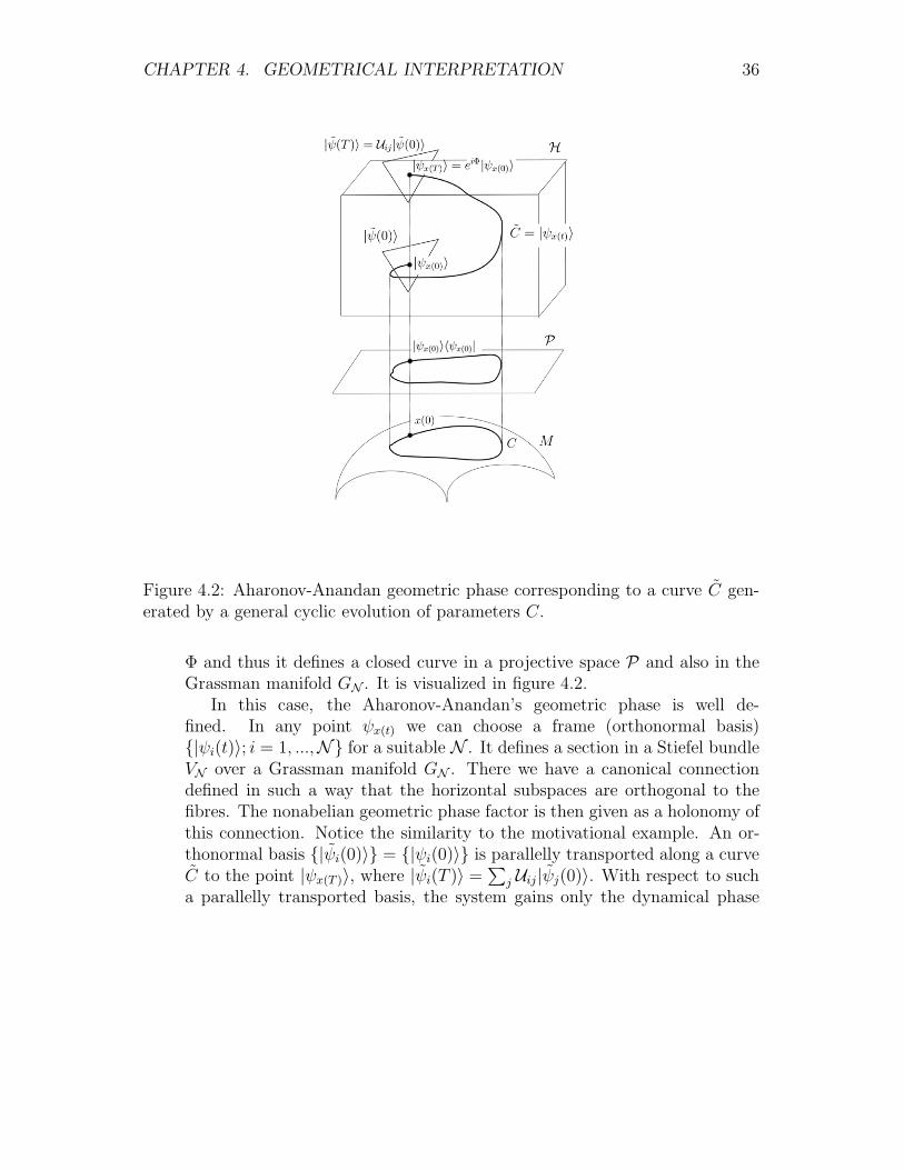
Figure 4.2: Aharonov-Anandan geometric phase corresponding to a curve C gen-erated by a general cyclic evolution of parameters C.

Φ and thus it defines a closed curve in a projective space P and also in theGrassman manifold GN . It is visualized in figure 4.2.

In this case, the Aharonov-Anandan’s geometric phase is well de-fined. In any point ψx(t) we can choose a frame (orthonormal basis)|ψi(t)〉; i = 1, ...,N for a suitable N . It defines a section in a Stiefel bundleVN over a Grassman manifold GN . There we have a canonical connectiondefined in such a way that the horizontal subspaces are orthogonal to thefibres. The nonabelian geometric phase factor is then given as a holonomy ofthis connection. Notice the similarity to the motivational example. An or-thonormal basis |ψi(0)〉 = |ψi(0)〉 is parallelly transported along a curveC to the point |ψx(T )〉, where |ψi(T )〉 =

∑j Uij |ψj(0)〉. With respect to such

a parallelly transported basis, the system gains only the dynamical phase


factor. The nonabelian geometric phase factor (holonomy transformation)Uij is given by the parallel transport.

But, we do not assume an adiabatic change of the parameter x andthus the frames |ψi(t)〉 is not posibble to choose being the eigenstatesof the Hamiltonians H(x) in general. Such an exact cyclic evolution (i.e.corresponding to a closed curve in the projective Hilbert space) allows ingeneral only the universal AA approach to the geometric phase. In the caseof a nonadiabatic evolution, we cannot define any BS bundle and we cannotuse the Berry’s adiabatic treatment. Although AA approach is very usefultheoretically, the BS approach is preferable for computation. The geometricphase, in the BS approach, is identified with the associated holonomy of theloops in the space of parameters and it means that one does not need to solvethe time dependent Schrodinger equation.

Moreover, it is not complicated to show ([24]) that an evolution given bySchrodinger equation can never be exactly described by any eigenprojectorΛ(x), i.e. the frames |ψi(t)〉 are never simultaneous eigenvectors of H(x).It means that the adiabatic condition is never exactly fulfilled and it can beonly a good approximation in some cases. Therefore it would be useful todevelope a Berry-like treatment for the geometric phase also for nonadiabaticevolutions, at least for some of them.

Suppose accordingly that we have such a physical system that the twofollowing conditions are satisfied:

1. The cyclic states are the eigenstates of a Hermitian operator H = H(x).

2. H is related to the Hamiltonian according to H(x) = H(F (x)), for a diffeo-morphism F : M →M .

For this class of quantum systems, one can still use the classification theorem.This is realized by replacing f by a map f defined by f = f F : M → GN .Then we obtain the (nonadiabatic) bundle λN over the parameter space M asthe pullback bundle λN = f ∗(ηN ). The map f also pullbacks the universalconnection Aij and yields a nonadiabatic Berry connection Aij = f ∗(Aij)on λN . The geometric phase is then obtainable as the holonomy of thisconnection

Uij = Pe∮ Aij = Pe

∮CAij(x) = Pe−

∮C〈ni(F (x))| ∂

∂xµ |nj(F (x))〉dxµ

.

In the adiabatic limit, F approaches to the identity map. Hence, F lies inthe connected component of Diff(M) and thus is homotopic to the identitymap. Therefore [f ] = [f ] and the bundles λN and λN have the same topology.


The conditions 1. and 2. seem to be quite restrictive. But, it turns outthat the first condition is fulfilled for any periodic Hamiltonian [17]. Neitherthe necessary nor the sufficient conditions for the existence of F for generalcyclic Hamiltonians are known, but there are examples where F exists andour analysis applies, e.g. the example of cranked Hamiltonian.

Chapter 5

Simple examples

In this section, I show how the formalism derivated in the previous chaptersapplies to simple examples. These, related to the adiabatic case are treatedmainly according to [22], [5] and [20]. In the nonadiabatic case, I follow thelines of [27] and [28].

5.1 The adiabatic nondegenerate case

Let me review the example of spin-12

particle in an external magnetic field.Assume that the Hamiltonian is given simply by H(x) = x · S, where x ∈R \ 0 and S is a spin-1

2operator ([Si, Sj] = iεijkSk) on C2. The actual

group G is obviously SU(2) and its representation on the Hilbert space is thestandard one. Thus the Hamiltonian can be parametrized by SU(2)/U(1).The Hamiltonian is already in the linear form and thus we know that can bediagonalized by an operator U(x) that is given by e−iz·S, where z3 = 0, i.e.U(x) is not generated by any element from the Cartan subalgebra. Our taskis to determine this operator, i.e. z. One can show that z ⊥ x has to holdand, finally, |z| = 1. The energy eigenvalues are precisely the eigenvalues sof the element S3 of the Cartan subalgebra, which are weights of the present,standard, representation. These are easy to be computed: s = −1

2, 0, 1

2. The

corresponding bundles are given by associating

x → |s(x)〉 := U(x)|s〉.The connection in this bundle is given by

As = −〈s|d(−iz · S)|s〉 = −i〈s|d(z1)S1 + d(z2)S2|s〉.

39

CHAPTER 5. SIMPLE EXAMPLES 40

I did not separate the terms coming from representation and the geometricalterms, because in such a nondegenerate case, we can use the Stoke’s theoremto proceed further. Using a spherical coordinate system one shows thatFs = sS(x), where S(x) is the ares form on the sphere in x. It means that atthe energy level E = 0, the Berry phase vanishes. For the energies E = ±1

2,

it is given by the solid angle formula γ± 12

= ±Ω(C).

5.2 The adiabatic degenerate case

An another nice example is the system described by the Hamiltonian H(x) =xiεijkσj ⊗ σk. Using, de facto, the same approach, one can compute theeigenvalues to be −2, 0, 2 and a further investigation reveals that the Berryphase vanishes for E = ±2. For the eigenvalue E = 0, which is two-degenerate, one obtains the Berry phase as a two times two diagonal matrixthat has precisely the terms ±Ω(C) on the diagonal [23].

A simple example of a nonabelian Berry phase is introduced in [5]. TheHamiltonian is considered to be given by H = R(t)HDR

−1(t), where HD isa constant diagonal matrix with nth times degenerate eigenvalue E = 0 andR(t) := R(θ(t)) is the SO(n+ 1) rotation, i.e.

R(θ) = eiθnTn,n+1 · · · eiθ2T2,n+1eiθ1T1,n+1

,

where Ti,n+1 are the generators of SO(n + 1)/SO(n). One of the intuitiveexplanation of the phenomenon of geometric phase can be such that theembedding of the relevant subgroup P into G varies in time, which canbe seen on this example. The parameter space is, of course, the sphereSn = SO(n+1)/SO(n) and the operator responsible for the geometric phaseis R(θ) now. The gauge potential is

Aij = −〈ni(θ)|d|nj(θ)〉

which is now a so(n)-valued form. For n = 3, we can find explicitly

A = sin θ1T12dθ2 + (sin θ1 cos θ2T13 + sin θ2T23) dθ3.

The berry phase is then, as usual, obtained as the integral Uij = −i ∮CAij .

A wide range of interesting adiabatic examples can be found and easilycomputed, see for instance [?].


5.3 The nonadiabatic case

Let us consider again a quantum system whose Hamiltonian is a function ofgenerators of a compact semisimple Lie group G. Then, as I explained inthe previous chapter, every Hamiltonian, which in the linear representationreads H0 = β · X, can be expressed as follows

H0 = εei∑

α∈∆+(zαXα+zαX−α) (a · H) e−i∑

α∈∆+(zαXα+zαX−α),

where a · H is an arbitrary element of the Cartan subalgebra. Supposethat the systems is initially in an eigenstate |m〉 of H, i.e. H|m〉 = m|m〉holds. Now, I will be concerned with a class of the systems with a crankedHamiltonian. It is such a time dependent Hamiltonian that arise from theinitial one by the adjoint action of a one-parameter group, i.e.

H(t) = e−iωtn·HH0eiωtn·H,

where ω is called the cranking rate and n the cranking direction.For such systems, the time dependent Schrodinger equation is exactly

solvable. It is due the fact that through a unitary transformation |ψ(t)〉 =e−iωtn·H|η(t)〉, we turn to the intrinsic frame. the evolution of |η(t)〉 is nowgoverned by the time independent Hamiltonian of the form

H(ω) = H0 − ωn · H = ε

(∑α

βαEα +∑i

(βi − ω

εni

)Hi

).

Then the state |ψ(t)〉 of the system evolves according to

|ψ(t)〉 = U(t)|ψ(0)〉 = e−iωtn·He−iH(ω)t|ψ(0)〉.Now, using the structure of semisimple compact algebras one compute

the final expression for the geometric phase [27] to be

ϕg = −2πn · m(

1 − 〈ηm|n · H|ηm〉n · m

).

This reveals that the phase is related to the expectation value of operatorsfrom Cartan algebra along the cranking direction n. Further, it dependson the geometry of parameter spaces n,m, on the ray ηm generated by theHamiltonian and on the cranking rate ω.


Let me come back to the example of a spin 12-particle in a rotating

magnetic field. It is obvious that this example belongs to the class witha cranked Hamiltonian. In this example, it is possible to proceed in a bitdifferent direction (as in [28]). Once we have constructed H(ω), we can definethe map F : S2 → S2 from the previous chapter by setting H(ω) ∝ H(F (x)).Thus it is given by equations

S2 (θ, ϕ) → (θ, ϕ) ∈ S2

cos θ =b

ω(cos θ − ω

b), sin θ =

b

ωsin θ, ϕ = ϕ.

But, one has to investigate if such defined map F is smooth. It need not beeven single valued. For this case, it is a diffeomorphims for every ω unlessthe Larmor frequency. Thus one obtains immediately the result

A = −k(1 − cos θ)dϕ

and the Berry phase is obtained from holonomy.

Chapter 6

Conclusion

In the first part of my work, I have introduced an example from the classicalphysics. Namely the example of the rotating globe. Although it does notrefer to the quantum mechanics, this example is quite illustrative. Thephenomenon, which here appears, is very similar to the one in quantummechanics. Namely, the additional angle of rotation, referred to as thegeometric phase, arises due to the parallel transport of the instantaneousbasis around a loop on the sphere which represents the globe. In fact, it is aconsequence of the curvature of sphere.

In the following, I have introduced the Berry’s, adiabatic, concept ofthe geometric phase and then the universal, Aharon-Anandan’s, approach.The geometric phases, defined in different way, are shown to be the samein the adiabatic limit. The construction of Aharon and Anandan has deeptheoretical implications, but do not provide any calculational useful formulas,because one has to solve the time independent Schrodinger equation. In thecase of Berry phase, there are such formulas accessible, but, on the otherhand, the adiabatic conditions are never exactly fulfilled.

Then, I have mentioned several experiments, which manifest the geomet-ric phase in rather different ways. In the case of coiled optical fibre, the localcurvature of the parameter space plays the crucial role and in the case ofAharon-Bohm effect, the nontriviality of the fundamental group of param-eter space is responsible for the additional phase factor. The example ofthree-level system is totally different in that the quantum state do not evolveaccording to the Schrodinger dynamics, but is made to evolve by adjustingsome parameters of interferometer. To conclude this part of my work, I haveintroduced some applications of the geometric phase.

43

CHAPTER 6. CONCLUSION 44

I have devoted the most effort to the fourth chapter, where I have focusedon the geometrical interpretation of the geometrical interpretation. There is anice similarity to the motivational example. Now, in he quantum mechanics,the geometric phase arise due to the parallel transport of the instantaneousbasis of Hilbert space. It is precisely the difference between the initial andthe transported basis, which is known as the holonomy. In the geometricinterpretation, the correspondence between the phase found by Berry and theone found by Aharon and Anandan becomes evident. For a given parameterspace, the possible bundles over it were classified. On the other hand, whenstarting with a (suitable) Hamiltonian, the possible spaces of parameterswere found. For the adiabatic case, I have further simplified the formulasfor the geometric phase using the structure of Lie algebras. Finally, I haveshowed that the Berry’s derivation can be used also in some nonadiabaticcases. As a conclusion, I have introduced several simple examples, whichillustrate the developed formalism.

Bibliography

[1] S. Pancharatnam, ”Generalized theory of interference and its applications”,Proc. Indian Acad. Sci. A 44 (1956) 247-262.

[2] M. V. Berry, ”Quantal phase factors accompanying adiabatic changes”, Proc.R. Soc. Lond. A 392 (1984) 45-57.

[3] Y. Aharonov and J. Anandan, ”Phase change during a cyclic quantum evolu-tion”, Phys. Rev. Lett. 58 (1987) 1593-1596.

[4] Arvind, K. S. Mallesh, N. Mukunda, ”A generalized Pancharatnam geometricphase formula for three-level quantum systems”, J. Phys. A 30 (1997) 2417-2431.

[5] F. Wilczek, A. Zee, ”Appearence of gauge structure in simple dynamicalsystems”, Phys. Rev. Lett. 52 (1984) 2111-2114.

[6] A. Tomita, R. Y. Chiao, ”Observation of Berry’s topological phase by use ofan optical fibre”, Phys. Rev. Lett. 57 (1986) 937-940.

[7] R. Y. Chiao, A. Antaramian, K.M. Ganga, H. Jiao, s.R. Wilkinson and H.Nathel, ”Observation of a topological phase by means of a nonplanar Mach-Zehnder interferometer”, Phys. Rev. Lett. 60 (1988) 1214-1217.

[8] T. Bitter and D. Dubbers, ”Manifestation of Berry’s topological in neutronspin rotation”, Phys. Rev. Lett. 59 (1987) 251-354.

[9] Y. Hasegawa, M. Zawisky, H. Rauch and A.I. Ioffe, ”Geometric phase incoupled neutron interference loops”, Phys. Rev. A 53 (1996) 2486-2492.

[10] R.Y. Chiao and Y.S. Wu, ”Manifestations of Bery’s topological phase for thephoton”, Phys. Rev. Lett. 57 (1986) 933-936.

45

BIBLIOGRAPHY 46

[11] Y. Aharonov, D. Bohm, ”Significance of electromagnetic potentials in thequantum theory”, Phys. Rev. 115, No. 3 (1959).

[12] B.C. Sanders, H. de Guise, S.D. Barlett, W. Zhang, ”Geometric phase ofthree-level systems in interferometry”, Phys. Rev. Lett. 86 (2001) 369-372.

[13] P.G. Kwiat, R.Y. Chiao, ”Observation of a nonclassical Berry’s phase for thephoton”, Phys. Rev. Lett. 66 (1991) 588-591.

[14] J. Anandan, L. Stodolsky, ”Some geometrical considerations of Berry’sphase”, Phys. Rev. D 35 (1987) 2597-2600.

[15] Allen Hatcher, book ”Algebraic topology” (2001).

[16] J.E. Avron, L. Sadun, J. Segert, B. Simon, ”Topological invariants in Fermisystems with time-reversal invariance”, Phys. Rev. Lett. 61 (1988) 1329-1332.

[17] A. Mostafazadeh, ”Geometric phase, bundle classification and group repre-sentation”, J. Math. Phys. 37 (1996) 1218-1233.

[18] K. Durstberger, ”Geometric phases in quantum theory” Diplomarbeit, Uni-Wien (2002).

[19] W. Fulton, J. Harris, book ”Representation theory”. Springer-Verlag (1991).

[20] B. Simon, ”Holonomy, the quantum adiabatic theorem, and Berry’s phase”,Phys. Rev. Lett. 51 2167-2169 (1983).

[21] N. Mukunda, ”Quantum kinematic approach to the geometric phase II. Thecase of unitary group representations”, Ann. of Phys. 228 (1993) 269-340.

[22] S. Giller, P. Kosinski and L. Szijmanowski, Int. J. Mod. Phys. A 4, 1453(1989).

[23] S. Giller, C. Gonera, P. Kosinski and P, Maslanka, Phys. Rev. A 48, 907-919(1993).

[24] A. Bohm, L.J. Boya, A. Mostafazadeh and G. Rudolph, ”Classification theo-rem for principal fibre bundles, Berry’s phase, and exact cyclic evolution”, J.of Geom. and Phys. 12 (1993) 13-28.

[25] N. Mukunda, ”Quantum kinematic approach to the geometric phase I. Gen-eral formalism”, Ann. of Phys. 228 (1993) 205-268.

BIBLIOGRAPHY 47

[26] M.A. Nielsen and I.L. Chuang, Quantum computation and quantum informa-tion. Cambridge University Press, Cambridge, 2000.

[27] S.J. Wang ”Nonadiabatic Berry’s phase for a quantum system with a dynam-ical semisimple Lie group”, Phys. Rev. A 42 (1990) 5103-5106.

[28] A. Mostafazadeh, A. Bohm, ”Topological aspects of the non-adiabatic Berryphase”, (1993) arXiv: hep-th/9309060.

[29] I. Kolar, P.W. Michor,J. Slovak, Natural operations in differential geometry,Springer-Verlag, 1993.

geometric phase in quantum theory - theor.physics.muni.cz

Documents