geometric model extraction from magnetic resonance volume data
TRANSCRIPT
Geometric Model Extraction fromMagnetic Resonance Volume Data
Thesis by
David H. Laidlaw
In Partial Fulfillment of the Requirements
for the Degree of
Doctor of Philosophy
California Institute of Technology
Pasadena, California
1995
(Defended May 23, 1995)

ii
Copyright c 1995David H. Laidlaw
All Rights Reserved
iii
Acknowledgments
This work was supported in part by grants from Apple, DEC, Hewlett Packard, and IBM. Additional
support was provided by NSF (ASC-89-20219) as part of the NSF/ARPA STC for Computer
Graphics and Scientific Visualization, by the DOE (DE-FG03-92ER25134) as part of the Center
for Research in Computational Biology, by the National Institute on Drug Abuse and the National
Institute of Mental Health as part of the Human Brain Project, and by the Beckman Institute
Foundation. All opinions, findings, conclusions, or recommendations expressed in this document
are those of the author(s) and do not necessarily reflect the views of the sponsoring agencies.
Matthew Avalos has been instrumental in implementing large parts of this work. Without his
dedication and incisive comments, this would have been smaller and taken a lot longer.
Thanks to Jose Jimenez for the late-night MR sessions and to Dr. Brian Ross for allowing
scanning time at the Huntington Magnetic Resonance Center in Pasadena, where some of our data
was collected.
I am grateful to Professor Alan Barr and his computer graphics group past and present: Cindy
Ball, Ronen Barzel, Allen Corcoran, Carolyn Collins, Bena Currin, Dan Fain, Louise Foucher, Kurt
Fleischer, Dave Kirk, Alf Mikula, Mark Montague, Preston Pfarner, John Snyder, Eric Winfree,
Adam Woodbury, and Denis Zorin. The lab folks provided a great environment together with lots
of collaborative help and advice.
My appreciation also goes to the MRI and Biology folks in the Beckman Institute at Caltech:
Erik Ahrens, John Allman, Andres Collazo, Hanan Davidowitz, Dian De Sha, Michael Figdor,
Mary Flowers, Scott Fraser, Pratik Ghosh, Russ Jacobs, Jim Narasimhan, Mark O’Dell, John Shih,

Acknowledgments iv
and Bill Trevarro. They provided me with many discussions of how MRI works and suggestions on
how I ought to be doing things.
Thanks to the readers of early drafts for their patience, stamina and very helpful suggestions:
Cindy Ball, Alan Barr, Ronen Barzel, Bena Currin, Dian De Sha, Dan Fain, David Kirk, Barbara
Meier, and Preston Pfarner.
I also want to express my appreciation to Charles and Patricia Laidlaw, my parents, for their
support and help throughout my time at Caltech.
And finally, thanks to my wife, Barbara Meier, for the moral and emotional support that helped
me make it through this long and sometimes arduous journey.
v
Abstract
This thesis presents a computational framework and new algorithms for creating geometric models
and images of physical objects. Our framework combines magnetic resonance imaging (MRI)
research with image processing and volume visualization. One focus is feedback of requirements
from later stages of the framework to earlier ones.
Within the framework we measure physical objects yielding vector-valued MRI volume datasets.
We process these datasets to identify different materials, and from the classified data we create
images and geometric models. New algorithms developed within the framework include a goal-
based technique for choosing MRI collection protocols and parameters and a family of Bayesian
tissue-classification methods.
The goal-based data-collection technique chooses MRI protocols and parameters subject to
specific goals for the collected data. Our goals are to make identification of different tissues
possible with data collected in the shortest possible time. Our method compares results across
different collection protocols, and is fast enough to use for steering the data-collection process.
Our new tissue-classification methods operate on small regions within a volume dataset, not
directly on the sample points. We term these regions voxels and assume that each can contain a
mixture of materials. The results of the classification step are tailored to make extraction of surface
boundaries between solid object parts more accurate.
Another new algorithm directly renders deformed volume data produced, for example, by
simulating the movement of a flexible body.
The computational framework for building geometric models allows computer graphics users

Abstract vi
to more easily create models with internal structure and with a high level of detail. Applications
exist in a variety of fields including computer graphics modeling, biological modeling, anatomical
studies, medical diagnosis, CAD/CAM, robotics, and computer animation. We demonstrate the
utility of the computational framework with a set of computer graphics images and models created
from data.
vii
Contents
Acknowledgments iii
Abstract v
Index of Figures xi
Availability xvi
1 Introduction 11.1 Motivation : : : : : : : : : : : : : : : : : : : : : : : : : : : : : : : : : : : : : 11.2 Model-Building Framework : : : : : : : : : : : : : : : : : : : : : : : : : : : : 2
1.2.1 Data Collection : : : : : : : : : : : : : : : : : : : : : : : : : : : : : : 21.2.2 Tissue Classification : : : : : : : : : : : : : : : : : : : : : : : : : : : : 51.2.3 Model Building and Visualization : : : : : : : : : : : : : : : : : : : : : 6
1.3 Overview : : : : : : : : : : : : : : : : : : : : : : : : : : : : : : : : : : : : : : 7
PART I. Data Collection 8
2 Goal-Based Data Collection 92.1 Introduction : : : : : : : : : : : : : : : : : : : : : : : : : : : : : : : : : : : : 11
2.1.1 Background and Motivation : : : : : : : : : : : : : : : : : : : : : : : : 112.1.2 Related Work : : : : : : : : : : : : : : : : : : : : : : : : : : : : : : : 122.1.3 Terminology : : : : : : : : : : : : : : : : : : : : : : : : : : : : : : : : 12
2.2 Conceptual Approach to Goal-Based Data Collection : : : : : : : : : : : : : : : 142.2.1 Optimization Framework : : : : : : : : : : : : : : : : : : : : : : : : : 152.2.2 Imaging Goals : : : : : : : : : : : : : : : : : : : : : : : : : : : : : : : 17
2.3 Mathematical Approach : : : : : : : : : : : : : : : : : : : : : : : : : : : : : : 182.3.1 Model of the MRI Process : : : : : : : : : : : : : : : : : : : : : : : : : 192.3.2 Imaging Goals : : : : : : : : : : : : : : : : : : : : : : : : : : : : : : : 222.3.3 Solving the Constrained Optimization Problem : : : : : : : : : : : : : : 24
2.4 Results : : : : : : : : : : : : : : : : : : : : : : : : : : : : : : : : : : : : : : : 252.4.1 Simulated Data : : : : : : : : : : : : : : : : : : : : : : : : : : : : : : 252.4.2 Real Data: Mouse Embryo : : : : : : : : : : : : : : : : : : : : : : : : : 282.4.3 Real Data: Dungeness Crab : : : : : : : : : : : : : : : : : : : : : : : : 31
2.5 Discussion : : : : : : : : : : : : : : : : : : : : : : : : : : : : : : : : : : : : : 35

Contents viii
2.5.1 Data Collected from Mouse Embryo : : : : : : : : : : : : : : : : : : : : 362.5.2 Data Collected from Dungeness Crab : : : : : : : : : : : : : : : : : : : 372.5.3 MRI Material and Collection Model : : : : : : : : : : : : : : : : : : : : 372.5.4 Choice of Protocol : : : : : : : : : : : : : : : : : : : : : : : : : : : : : 382.5.5 Choice of Contrast-to-Noise Ratio (CNR) : : : : : : : : : : : : : : : : : 392.5.6 Solver : : : : : : : : : : : : : : : : : : : : : : : : : : : : : : : : : : : 40
2.6 Conclusion : : : : : : : : : : : : : : : : : : : : : : : : : : : : : : : : : : : : : 41
PART II. Bayesian Tissue Classification 42
3 Bayesian Tissue-Classification Framework 433.1 Introduction : : : : : : : : : : : : : : : : : : : : : : : : : : : : : : : : : : : : 45
3.1.1 Related Work : : : : : : : : : : : : : : : : : : : : : : : : : : : : : : : 453.1.2 Definitions : : : : : : : : : : : : : : : : : : : : : : : : : : : : : : : : : 45
3.2 A Framework for Solutions : : : : : : : : : : : : : : : : : : : : : : : : : : : : 463.2.1 Bayesian Construction of Material Probabilities : : : : : : : : : : : : : : 473.2.2 Classification : : : : : : : : : : : : : : : : : : : : : : : : : : : : : : : 513.2.3 Example of Classification Algorithm Construction : : : : : : : : : : : : 51
3.3 A Family of Solutions : : : : : : : : : : : : : : : : : : : : : : : : : : : : : : : 533.3.1 Assumptions Common to New Algorithms : : : : : : : : : : : : : : : : 533.3.2 Voxel-info: Histograms : : : : : : : : : : : : : : : : : : : : : : : : : : 543.3.3 Overview of Algorithm A: Partial Volume Mixtures : : : : : : : : : : : : 553.3.4 Overview of Algorithm B: Boundary Distance : : : : : : : : : : : : : : : 563.3.5 Overview of Algorithm C: Boundary Distance with Non-Uniform Material
Signatures : : : : : : : : : : : : : : : : : : : : : : : : : : : : : : : : : 573.4 Summary : : : : : : : : : : : : : : : : : : : : : : : : : : : : : : : : : : : : : : 58
4 Bayesian Classification Algorithm A: Partial Volume Mixtures 594.1 Construction : : : : : : : : : : : : : : : : : : : : : : : : : : : : : : : : : : : : 60
4.1.1 Voxel-info : : : : : : : : : : : : : : : : : : : : : : : : : : : : : : : : : 614.1.2 Assumptions : : : : : : : : : : : : : : : : : : : : : : : : : : : : : : : : 614.1.3 Sketch of Derivation : : : : : : : : : : : : : : : : : : : : : : : : : : : : 62
4.2 Algorithm : : : : : : : : : : : : : : : : : : : : : : : : : : : : : : : : : : : : : 624.3 Normalized Histograms : : : : : : : : : : : : : : : : : : : : : : : : : : : : : : 644.4 Histogram Basis Functions for Pure Materials and Mixtures : : : : : : : : : : : : 664.5 Estimating Dataset Parameters : : : : : : : : : : : : : : : : : : : : : : : : : : : 674.6 Classification: Estimating Voxel Parameters : : : : : : : : : : : : : : : : : : : : 684.7 Results : : : : : : : : : : : : : : : : : : : : : : : : : : : : : : : : : : : : : : : 694.8 Discussion : : : : : : : : : : : : : : : : : : : : : : : : : : : : : : : : : : : : : 714.9 Conclusion : : : : : : : : : : : : : : : : : : : : : : : : : : : : : : : : : : : : : 754.10 Derivation of Material PDFs : : : : : : : : : : : : : : : : : : : : : : : : : : : : 75
4.10.1 Pure Materials : : : : : : : : : : : : : : : : : : : : : : : : : : : : : : : 764.10.2 Mixtures : : : : : : : : : : : : : : : : : : : : : : : : : : : : : : : : : : 76
4.11 Derivation of Classification Parameter Estimation : : : : : : : : : : : : : : : : : 774.11.1 Definitions : : : : : : : : : : : : : : : : : : : : : : : : : : : : : : : : : 774.11.2 Optimization : : : : : : : : : : : : : : : : : : : : : : : : : : : : : : : : 78
Contents ix
4.11.3 Derivation of the posterior probability P(�; c; s; �Njh) : : : : : : : : : : : 78
5 Bayesian Classification Algorithms B and C: Boundary Distance 825.1 Assumptions : : : : : : : : : : : : : : : : : : : : : : : : : : : : : : : : : : : : 835.2 Histogram Basis Functions : : : : : : : : : : : : : : : : : : : : : : : : : : : : : 845.3 Estimating Dataset Parameters : : : : : : : : : : : : : : : : : : : : : : : : : : : 86
5.3.1 Non-uniform Material Signatures : : : : : : : : : : : : : : : : : : : : : 875.4 Estimating Voxel Parameters : : : : : : : : : : : : : : : : : : : : : : : : : : : : 875.5 Results : : : : : : : : : : : : : : : : : : : : : : : : : : : : : : : : : : : : : : : 885.6 Discussion : : : : : : : : : : : : : : : : : : : : : : : : : : : : : : : : : : : : : 905.7 Conclusion : : : : : : : : : : : : : : : : : : : : : : : : : : : : : : : : : : : : : 915.8 Detailed Derivations : : : : : : : : : : : : : : : : : : : : : : : : : : : : : : : : 92
5.8.1 Pure Histogram Basis Function : : : : : : : : : : : : : : : : : : : : : : 925.8.2 Mixture Histogram Basis Function : : : : : : : : : : : : : : : : : : : : 925.8.3 Pure Material Parameter Estimation : : : : : : : : : : : : : : : : : : : : 945.8.4 Material Mixture Parameter Estimation : : : : : : : : : : : : : : : : : : 95
PART III. Applications 98
6 Model Building 996.1 Taxonomy of Computer Graphics Models : : : : : : : : : : : : : : : : : : : : : 1006.2 Modeling Examples : : : : : : : : : : : : : : : : : : : : : : : : : : : : : : : : 101
6.2.1 Static Surface Models : : : : : : : : : : : : : : : : : : : : : : : : : : : 1026.2.2 Static Volume Models : : : : : : : : : : : : : : : : : : : : : : : : : : : 1056.2.3 Dynamic Models : : : : : : : : : : : : : : : : : : : : : : : : : : : : : : 106
6.3 Conclusion : : : : : : : : : : : : : : : : : : : : : : : : : : : : : : : : : : : : : 109
7 Deformed Volume Rendering 1107.1 Introduction : : : : : : : : : : : : : : : : : : : : : : : : : : : : : : : : : : : : 110
7.1.1 Related Work : : : : : : : : : : : : : : : : : : : : : : : : : : : : : : : 1117.1.2 Our Approach : : : : : : : : : : : : : : : : : : : : : : : : : : : : : : : 1127.1.3 Overview : : : : : : : : : : : : : : : : : : : : : : : : : : : : : : : : : 113
7.2 Terms and Definitions : : : : : : : : : : : : : : : : : : : : : : : : : : : : : : : 1137.2.1 Interval Methods : : : : : : : : : : : : : : : : : : : : : : : : : : : : : : 1137.2.2 Volume Rendering : : : : : : : : : : : : : : : : : : : : : : : : : : : : : 1147.2.3 Deformations : : : : : : : : : : : : : : : : : : : : : : : : : : : : : : : 115
7.3 Algorithm : : : : : : : : : : : : : : : : : : : : : : : : : : : : : : : : : : : : : 1167.3.1 Finding All Boundary Intersections : : : : : : : : : : : : : : : : : : : : 1187.3.2 Calculating the Path Through the Dataset : : : : : : : : : : : : : : : : : 1207.3.3 Implementation Considerations : : : : : : : : : : : : : : : : : : : : : : 120
7.4 Results : : : : : : : : : : : : : : : : : : : : : : : : : : : : : : : : : : : : : : : 1227.5 Conclusion : : : : : : : : : : : : : : : : : : : : : : : : : : : : : : : : : : : : : 1227.6 Derivation of Deformed Path : : : : : : : : : : : : : : : : : : : : : : : : : : : : 123
8 Conclusions and Future Work 1258.1 Conclusions : : : : : : : : : : : : : : : : : : : : : : : : : : : : : : : : : : : : 125

Contents x
8.1.1 Goal-based Data Collection : : : : : : : : : : : : : : : : : : : : : : : : 1268.1.2 Bayesian Classification : : : : : : : : : : : : : : : : : : : : : : : : : : 1268.1.3 Model-Building and Visualization : : : : : : : : : : : : : : : : : : : : : 1278.1.4 Interaction of Framework Stages : : : : : : : : : : : : : : : : : : : : : : 127
8.2 Extensions : : : : : : : : : : : : : : : : : : : : : : : : : : : : : : : : : : : : : 1288.2.1 Goal-based Data Collection : : : : : : : : : : : : : : : : : : : : : : : : 1288.2.2 Artifacts in MRI Data : : : : : : : : : : : : : : : : : : : : : : : : : : : 1298.2.3 Classification : : : : : : : : : : : : : : : : : : : : : : : : : : : : : : : 1308.2.4 Model Building and Simulation : : : : : : : : : : : : : : : : : : : : : : 1318.2.5 Volume Rendering : : : : : : : : : : : : : : : : : : : : : : : : : : : : : 131
8.3 Summary : : : : : : : : : : : : : : : : : : : : : : : : : : : : : : : : : : : : : : 132
Bibliography 133

xi
Index of Figures
Ch. 1. Introduction
1.1
Real World Objects
Sampled Volume Data (MR, CT)
Identi�ed Materials
Geometric/Dynamic Models Images/Animation
Data Collection
Classi�cation
ModelBuilding
Volume Rendering/
Visualization
??
??
@@@R
@@@R
���
���
: 3
Geometric model buildingframework
Ch. 2. Goal-Based Data Collection
2.1
Real World Objects
Sampled Volume Data (MR, CT)
Identi�ed Materials
Geometric/Dynamic Models Images/Animation
Data Collection
Classi�cation
ModelBuilding
Volume Rendering/
Visualization
??
??
@@@R
@@@R
���
���
: 10
Goal-based collection context
2.2
radiofrequency pulses
slicegradient
phaseencodinggradient
frequencyencodinggradient
signal
sweepwidth,
encode time
tipangle
maxgradient
time
FOV, N0
FOV, N1
echo time,
slice locationand thickness
ETrecycle time, RT
SW
ET /2 ET /2
: 13
Pulse program
2.3 Collect Images
Interactive --- Once
Automatic --- Iterated
Choose NewParameters
Guess Parameters
Specify Imaging Goals CollectionParameters
ImagesImaging Goals
Start
Doneok? yes
no
Images : 15
Data collection optimizationprocess
2.4
Estimate material parameters
material model
ImagesImagingGoals
Predict material signatures
material signatures
Calculate objective function
objective function
ok?
Select collection parameters
collectionparameters
no
yes
CollectionParameters
Choose
New
Parameters: 16
Data collection “inner loop”
2.5
Prob
abili
ty D
ensi
ty
MRI Value
Prob
abili
ty D
ensi
ty
MRI Value
: 18
“Good enough” data
2.6 : 26
Shape of simulated data
2.7TE (ms)
10
16.7
23.3
30
TR (ms)700567433300
: 26
Simulated data
2.81000
20003000
40005000
50 100 150 200 250
23456789
10
TR
TE (Na = 3)
log(E())
10002000
30004000
500050 100 150 200 250
23456789
10
TR
TE (Na = 4)
log(E())
: 27
Objective function for simulateddata
2.90
0.001
0.002
0.003
0.004
0.005
0.006
0.007
0 200 400 600 800 1000 1200 1400
Prob
abili
ty D
ensi
ty
MRI Value (TR/TE = 700/10)
data histogrampredicted material 1 distribution
predicted material 2 distributionpredicted material 3 distribution (air)
: 28
Simulated data before optimization

Index of Figures xii
2.100
0.002
0.004
0.006
0.008
0.01
0 100 200 300 400 500 600 700 800 900
Prob
abili
ty D
ensi
ty
MRI Value (TR/TE = 1278/109)
data histogrampredicted material 1 distributionpredicted material 2 distribution
predicted material 3 distribution (air)
: 28
Simulated data post optimization
2.11
TE (ms)
08
16
32
64
128
TR(ms)
32001600800400200100Na: 2
: 29
Phantom data
2.121
23 4
5
: 29
Diagram of mouse embryo regions
2.130
10002000
30004000
50000 50 100
0
5
10
15
TR
TE (Na = 38)
log(E())
: 31
Objective function for mouseembryo
2.14(i) (ii)
(iii) (iv)
: 32
Data collected for differentoptimization steps
2.15TE (ms)
20
40
60
80
125
250
375
500
TR(ms): 1000300300100
Na: 1121
: 33
Crab data
2.160
5001000
15002000
25003000
35004000
45000 50 100
0123456789
10
TR
TE (Na = 1)
log(E())
: 34
Objective function for crab data
2.17 : 34
Crab data post optimization
2.18
0
200
400
600
800
1000
1200
1400
0 200 400 600 800 1000 1200
MR
I V
alue
2
MRI Value 1
optimal predictedpredicted
data
: 35
Crab data values before and afteroptimization
2.19
iter 1
iter 2
iter 3
iter 4
iter 5
0 200 400 600 800 1000 1200 1400 1600 18003
3p
4
4p
5
5p
"measured""predicted"
: 36
Predicted and measured means anddeviations
2.20
0
50
100
150
200
250
300
5 10 15 20 25 30 35 40
Tim
e (m
in)
Goal CNR
: 39
Collection time vs. CNR
Ch. 3. Bayesian Tissue-ClassificationFramework
3.1
Real World Objects
Sampled Volume Data (MR, CT)
Identi�ed Materials
Geometric/Dynamic Models Images/Animation
Data Collection
Classi�cation
ModelBuilding
Volume Rendering/
Visualization
??
??
@@@R
@@@R
���
���
: 44
Tissue-classification context
3.2 sample
voxel
volume dataset
: 46
Samples and voxels

Index of Figures xiii
3.34.1.1. Bayesian Construction
4.1.2. Classification
Raw MRI Data
Material/MixtureProbability Equations
Classified Data
Assumptionsabout measurementprocess and object
: 47
Steps in creating and using a newBayesian classifier.
3.4
Freq
uenc
y
Image intensity
Pure APure B
Pure C
A&BA&C
B&C
(i)
(ii)
(iii)
(iv)
: 48
Benefits of vector-valued data
Ch. 4. Bayesian Classification AlgorithmA: Partial Volume Mixtures
4.1
A
B
P1
P2
P3
(i)
A
B
A&B
P1
P2
P3
(ii)
: 60
Assumptions for mixtureclassification
4.2
Volume Ratio Densities
Sampled MR Data
Fitted Histogram
Whole Dataset Histogram, h (v)
Histograms of Voxel-sizedRegions, h (v)
Real World Object
FittedHistograms
all
vox : 63
Steps in the classification process
4.3
vA
vB
Histogram
Measurement
Histogram
A & B
A
B
A
B
vA
vB
Position
Position
Measurement
(i)
(ii)
: 65
Noise and mixtures in histograms
4.4c
s
Single Material PDF Two-Material PDF
c 0 c 1
s1 s0
(i) (ii)
: 66
Parameters of single-material PDF
4.5
(i) Geometry of slices
(ii) \Ideal"classi�cation
(iii) Discreteclassi�cation(no mixtures)
(iv) Continuous,multi-materialclassi�cation
(v) Original simulated two-valued data
: 70
Classification results on simulateddata
4.6 : 71
Discrete classification of brainslice
4.7(i) Original Data
(ii) Results of AlgorithmClassi�ed White Matter (white), Gray Matter (gray)
Cerebro-Spinal Fluid (blue), Muscle (red)
(iii) Combined Classi�ed Image
: 72
Classified brain slice
4.8 : 73
Histogram fit with PDFs
4.9 : 73
Volume-rendered classified handdataset

Index of Figures xiv
Ch. 5. Bayesian Classification AlgorithmsB and C: Boundary Distance
5.1
A
B
P1
P2
P3
(i)
A
B
P1
P2
P3
kw
d
(ii)
: 85
Assumptions for boundarydistance classification
5.2
0
0.05
0.1
0.15
0.2
0.25
0.3
0.35
5 10 15 20
f bo
unda
ry(v
)
MRI value, v c1=5, c2=20, s=3, Kw=0.4
d=0
d=0.6d=-0.6
d=0.9d=-0.9
: 85
Boundary histogram basisfunctions
5.3
d=0.9d=-0.6
d=0.1
c1=(5,5), c2=(15,25), s=(3,5), Kw=0.4
510
1520
5 10 15 20 25
00.010.020.030.040.050.060.070.08
MRI value, v1
MRI value, v2
f boundary(v1, v2)
: 86
Boundary histogram basis functionfor vector-valued data
5.4
(i) Geometry ofslices
(ii) Raw data
Mat. 1:
Mat. 2:
Mat. 3:
(iii) \Ideal"classi�cation
(iv) Discreteclassi�cation(vector)
(v) Partial volumemixture
classi�cation(vector)
(vi) Boundarydistance
classi�cation(scalar)
: 89
Classification results on simulateddata
Ch. 6. Model Building
6.1
Real World Objects
Sampled Volume Data (MR, CT)
Identi�ed Materials
Geometric/Dynamic Models Images/Animation
Data Collection
Classi�cation
Model Volume Rendering/Building Visualization
??
??
@@@R
@@@R
���
���
: 100
Model-building and visualizationcontext
6.2 : 102
Rigid model of external surface ofa lobster
6.3 : 103
Rigid model of external surface ofa lobster
6.4
1
: 103
Geometric model of tooth dentineand enamel
6.5 : 104
MRI data of a human molar
6.6 : 105
Model of a bear
6.7 : 106
Model of a bee
6.8 : 106
Volume model of a human hand
6.9 : 107
Flexible deformation of jade plant
Index of Figures xv
6.10
1
: 107
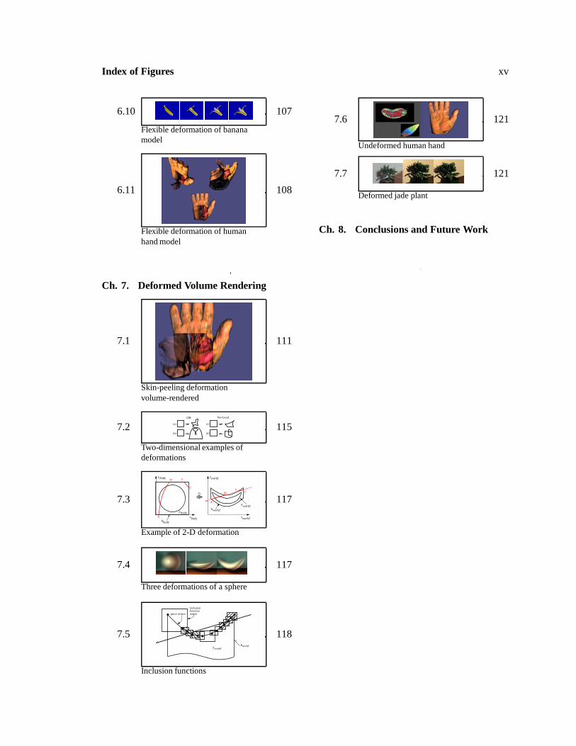
Flexible deformation of bananamodel
6.11 : 108
Flexible deformation of humanhand model
Ch. 7. Deformed Volume Rendering
7.1 : 111
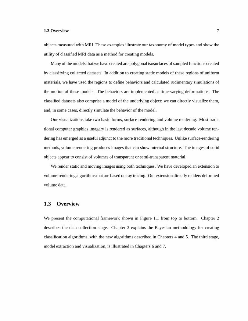
Skin-peeling deformationvolume-rendered
7.2 (a)
(b)
(c)
(d)
OK No Good
: 115
Two-dimensional examples ofdeformations
7.3U
VW
X
xworld
S worldbworld
D
xbody
U
VW
X
S body
bbody
y body yworld
: 117
Example of 2-D deformation
7.4
1
: 117
Three deformations of a sphere
7.5S world
bworld
Inclusionfunctionoutputpiece of face
: 118
Inclusion functions
7.6 : 121
Undeformed human hand
7.7
1
: 121
Deformed jade plant
Ch. 8. Conclusions and Future Work

xvi
Availability
Paper copies of this thesis are available by U.S. mail to:
Computer Science LibraryCaltech M/S 256-80Pasadena, CA 91125
The library also maintains an online version on the World Wide Web. The URL of the index of
available technical reports is:
file://cs.caltech.edu/tr/INDEX.html
Many of the images are also online. Start at my home page:
http://www.gg.caltech.edu/�dhl/phd.html
I can be reached via e-mail to [email protected].

1
Chapter 1
Introduction
1.1 Motivation
Computer graphics is a broad field. Its practitioners gather within it any domain in which images
are generated or enhanced by a computer. One thrust within computer graphics is the creation of
models and images of objects such as plants or animals to further our understanding of them. The
same types of models and images also have applications in entertainment and education.
Our work explores some new techniques for studying anatomy, development, and behavior
through this modeling and rendering process. Given a locust, a human hand, or a frog embryo, how
can we visualize and understand it? What new tools are needed to answer questions about it?
We present a computational framework for attacking some of the difficulties in making models
and images. Our framework is centered around measuring objects, identifying different regions
within the objects, and creating images and models using information about the regions and mea-
surements.
The framework is not a one-way pipeline. Instead, each stage requires input with certain

1.2 Model-Building Framework 2
characteristics; these required characteristics impact the output of earlier stages. The feedback
assures that the output from each stage meets the requirements for input to the next.
In this chapter we present our computational framework, discuss some of the novel techniques
that we have developed within the framework, and give an overview of the remaining chapters.
1.2 Model-Building Framework
Our framework consists of three main stages, illustrated in Figure 1.1. In the first stage, data
collection and processing, real-world objects are measured and the resulting sampled volume data
processed and stored for later stages. We describe some of the problems and our approaches to
solving them in Section 1.2.1 and in Chapter 2.
The second stage of the framework, classification, identifies regions containing different mate-
rials within the objects we have measured. The sampled volume data is used as input. Section 1.2.2
and Chapter 3 describe our Bayesian methodology for generating classification algorithms, and
Chapters 4 and 5 present three new algorithms.
The third stage of the framework, model building and visualization, generates models, images,
and animations of our objects. We outline some of the challenges and show results of applying our
techniques to classified MRI data in Section 1.2.3 and in Chapters 6 and 7.
1.2.1 Data Collection
In the first stage of our computational framework we measure the physical object we wish to model.
The data we collect must distinguish different materials sufficiently for our classification and model-
extraction processes to work. We have developed techniques that help us to collect data that satisfies
our imaging goals in a minimal amount of time.
Why MRI? We have chosen to use magnetic resonance imaging (MRI) for a number of reasons.
First, MRI measures information about both the inside and the outside of an object. The resulting

1.2 Model-Building Framework 3
Real World Objects
Sampled Volume Data (MR, CT)
Identi�ed Materials
Geometric/Dynamic Models Images/Animation
Data Collection
Classi�cation
ModelBuilding
Volume Rendering/
Visualization
??
??
@@@R
@@@R
���
���
Figure 1.1: This figure shows the computational framework that we use for creating static and dynamic geometric modelsfrom MRI data. 2
volume data identify internal structure, an important factor in the behavior of dynamic models.
Second, MRI measures at least three independent parameters of each material, and so has the
potential to distinguish more different materials than techniques that measure only a single parameter.
Third, it is not invasive, so we can measure living plants and animals without damaging them. Fourth,
although imaging time is expensive, MRI is accessible at most large hospitals and at imaging centers.
Other modalities have been used for creating models. Laser range-scanning is the most
widespread [Turk and Levoy, 1994] primarily due to its low cost and high level of detail. It is,
however, limited to line-of-sight surface measurements, which are sufficient for many static com-
puter graphics applications, but not sufficient for applications requiring internal structure or for
dynamic models where an initially invisible portion of the surface may become visible.

1.2 Model-Building Framework 4
Computed tomography (CT) data have also been used for similar purposes [Drebin et al., 1988].
CT can produce higher-resolution data than MRI and measures internal structure, but suffers from
two drawbacks. First, it uses ionizing x-radiation, which damages living tissues; and second, its
measurements depend only on a single material parameter, and so cannot differentiate tissues as
well as MRI.
Limitations. MRI datasets have a number of limitations. There are many different MRI methods
or protocols for collecting data, each with a set of parameters that influence how different materials
appear in the resulting images. Choosing a protocol and parameters from this panoply is a formidable
task, often requiring years of experience and frequently only moderately successful. Further
complicating the problem, MRI collections are time-limited by the physics of the spinning hydrogen
nuclei; datasets with a large enough signal-to-noise ratio or contrast-to-noise ratio often require a
prohibitive amount of time to collect.
There are also many distortions that can appear in MRI data. Broadly, the distortions can be
categorized as geometry or intensity related. We avoid some of the distortions by constraining the
data-collection process and reduce others through the parameter optimization process. In a post-
collection step we reduce even more through image-processing techniques. We defer attending to
some of the distortions until the tissue-classification stage where we diminish the artifacts through
new classification algorithms.
Cost and accessibility are additional issues. While MRI machines exist in most large hospitals
and in imaging centers in many large cities, they are expensive to use, currently costing around
$400-1000/hour, and often difficult to access.
MRI Data Collection Parameter Setting. As we describe in more detail in Section 2.1.2, others
have attacked the MRI parameter-setting problem with techniques that optimize the contrast between
two specific materials or that find closed-form solutions for a specific protocol. Some numerical
techniques have also been used to optimize the contrast-to-noise ratio for a particular collection

1.2 Model-Building Framework 5
algorithm.
In Chapter 2 we directly address the parameter-setting and collection-time problems by codifying
the requirements of the classification, model-building, and visualization algorithms; the complex
constraints of the MRI machines; and the desire to reduce collection time. From the requirements
we construct a mathematical optimization problem that we solve numerically to find collection
parameters that collect data satisfying our requirements in the shortest possible time.
1.2.2 Tissue Classification
The second stage in our computational framework involves classifying or segmenting our sampled
datasets to identify regions of different materials within the datasets. The main motivation for our
classification work is to make computer graphics models and images using volume measurements
of physical objects. Identifying different materials is a key step in the process, particularly when
different materials have different behaviors or appearances. Computer graphics applications include
volume-rendered images [Levoy, 1988], surface models [Lorensen and Cline, 1987], and volume models
created from the data.
Applications of the models and images include surgical planning and assistance, conventional
computer animation, anatomical studies, and predictive modeling of complex biological shapes and
behavior. Some aspects of our classification techniques could also be applied to medical diagnosis.
With further development, the concepts may also apply to computer vision problems or to extracting
mattes for digital optical effects.
Sources of sampled volume data are becoming more numerous and accessible. In addition
to MRI, they include Computed Tomography (CT), as well as astrophysical, meteorological, and
geophysical measurements. The computational sciences frequently produce sampled output, e.g.,
the results of computational fluid dynamics (CFD) and finite element method (FEM) simulations.
We have focused on classifying MRI data, but our techniques apply to other modalities as well.
We describe related classification work in Section 3.1.1. In some of this work classification is
implemented via interactively selected mappings from data values to colors and opacities, which

1.2 Model-Building Framework 6
are then rendered, or via interactively chosen threshold values for distinguishing regions. Many
more rigorous classification algorithms have also been developed, but are of limited applicability to
classifying sampled MRI data for extracting models.
Bayesian Framework. We have developed a methodology (see Chapter 3) for constructing a
Bayesian classification algorithm from a set of assumptions about the underlying data. Our algo-
rithms start with the premise that the sampled datasets satisfy the Nyquist sampling theorem, which
allows us to reconstruct a continuous function �(x) over the entire dataset [Oppenheim et al., 1983].
We calculate histograms of �(x) over small regions of the dataset and classify those histograms by
fitting histogram basis functions constructed from the set of assumptions.
Classification Algorithms. Using the Bayesian framework we have constructed three different
classification algorithms, described in more detail in Chapters 4 and 5. The first algorithm models
each voxel as a linear combination of pure materials and mixtures of two materials. The second
algorithm models each voxel as either entirely composed of a single pure material, or composed of
a mixture between two materials with a boundary between those two materials. The third algorithm
is substantially similar to the second, but allows the expected value, or signature, of each material
to vary over a dataset, a common characteristic of MRI data. These techniques classify MRI data
better than previously available techniques because they use a more accurate model of the collected
data. They are also tailored to produce accurate results near boundaries between materials where
extracted model details are most visible.
1.2.3 Model Building and Visualization
The final stage in our computational framework involves extracting geometric and dynamic models
and visualizing the results. We describe this work in Chapters 6 and 7. We have primarily
experimented with applying existing techniques to the data that we have collected and classified.
Using these techniques we have created a series of models and images of inanimate and animate
1.3 Overview 7
objects measured with MRI. These examples illustrate our taxonomy of model types and show the
utility of classified MRI data as a method for creating models.
Many of the models that we have created are polygonal isosurfaces of sampled functions created
by classifying collected datasets. In addition to creating static models of these regions of uniform
materials, we have used the regions to define behaviors and calculated rudimentary simulations of
the motion of these models. The behaviors are implemented as time-varying deformations. The
classified datasets also comprise a model of the underlying object; we can directly visualize them,
and, in some cases, directly simulate the behavior of the model.
Our visualizations take two basic forms, surface rendering and volume rendering. Most tradi-
tional computer graphics imagery is rendered as surfaces, although in the last decade volume ren-
dering has emerged as a useful adjunct to the more traditional techniques. Unlike surface-rendering
methods, volume rendering produces images that can show internal structure. The images of solid
objects appear to consist of volumes of transparent or semi-transparent material.
We render static and moving images using both techniques. We have developed an extension to
volume-rendering algorithms that are based on ray tracing. Our extension directly renders deformed
volume data.
1.3 Overview
We present the computational framework shown in Figure 1.1 from top to bottom. Chapter 2
describes the data collection stage. Chapter 3 explains the Bayesian methodology for creating
classification algorithms, with the new algorithms described in Chapters 4 and 5. The third stage,
model extraction and visualization, is illustrated in Chapters 6 and 7.

8
PART I
Data Collection
The following part of the thesis describes goal-based data collection, a tech-
nique for choosing a specific MRI collection technique and specific collection
parameters from the myriad of possibilities. The choice is guided by a series of
goals for the resulting volume data and the collection process.
9
Chapter 2
Goal-Based Data Collection
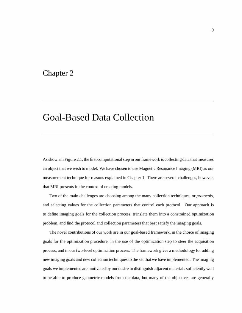
As shown in Figure 2.1, the first computational step in our framework is collecting data that measures
an object that we wish to model. We have chosen to use Magnetic Resonance Imaging (MRI) as our
measurement technique for reasons explained in Chapter 1. There are several challenges, however,
that MRI presents in the context of creating models.
Two of the main challenges are choosing among the many collection techniques, or protocols,
and selecting values for the collection parameters that control each protocol. Our approach is
to define imaging goals for the collection process, translate them into a constrained optimization
problem, and find the protocol and collection parameters that best satisfy the imaging goals.
The novel contributions of our work are in our goal-based framework, in the choice of imaging
goals for the optimization procedure, in the use of the optimization step to steer the acquisition
process, and in our two-level optimization process. The framework gives a methodology for adding
new imaging goals and new collection techniques to the set that we have implemented. The imaging
goals we implemented are motivated by our desire to distinguish adjacent materials sufficiently well
to be able to produce geometric models from the data, but many of the objectives are generally

Chapter 2. Goal-Based Data Collection 10
Real World Objects
Sampled Volume Data (MR, CT)
Identi�ed Materials
Geometric/Dynamic Models Images/Animation
Data Collection
Classi�cation
ModelBuilding
Volume Rendering/
Visualization
??
??
@@@R
@@@R
���
���
Figure 2.1: Our computational framework for creating geometric models, as shown earlier in Figure 1.1. In Chapter 2 wedescribe our goal-based data-collection process, emphasized in the diagram. Our new techniques help select an optimalcollection technique and set of collection parameters given a set of imaging goals for the resulting volume data. 2
applicable to imaging applications. These imaging goals differ from other work in that they do not
find collection parameters yielding the most contrast or highest contrast-to-noise ratio (CNR), but
rather find parameters yielding sufficient contrast in the least amount of time. Also, any number
of materials can be specified by a user from a low-resolution dataset, and optimal parameters are
generated taking into account inherent machine limitations and desired collection parameters such
as resolution. Finally, because units of the function we optimize are consistent from protocol to
protocol, we can choose the most appropriate technique or combination of techniques. We can even
choose between collections that produce scalar or vector-valued data.
We validate our technique with results using simulated as well as real MRI data.
The chapter is organized as follows: Section 2.1.1 discusses the collection of MRI data and
2.1 Introduction 11
motivates the need for goal-based collection techniques. Section 2.1.2 describes related work in the
area and compares it to our work. We define terms in Section 2.1.3. In Section 2.2 we describe
our imaging goals and give a conceptual description of the optimization process. A mathematical
description follows in Section 2.3 with results, discussion, and conclusions in Sections 2.4–2.6.
2.1 Introduction
2.1.1 Background and Motivation
Collecting good MRI data is difficult because imaging systems are very sensitive to the many
parameters of the various collection techniques, to the choice of technique, to subtle differences in
the materials that are being imaged, and to the fine tuning of the machine being used. Many parts
of the process are also inherently analog and difficult to calibrate.
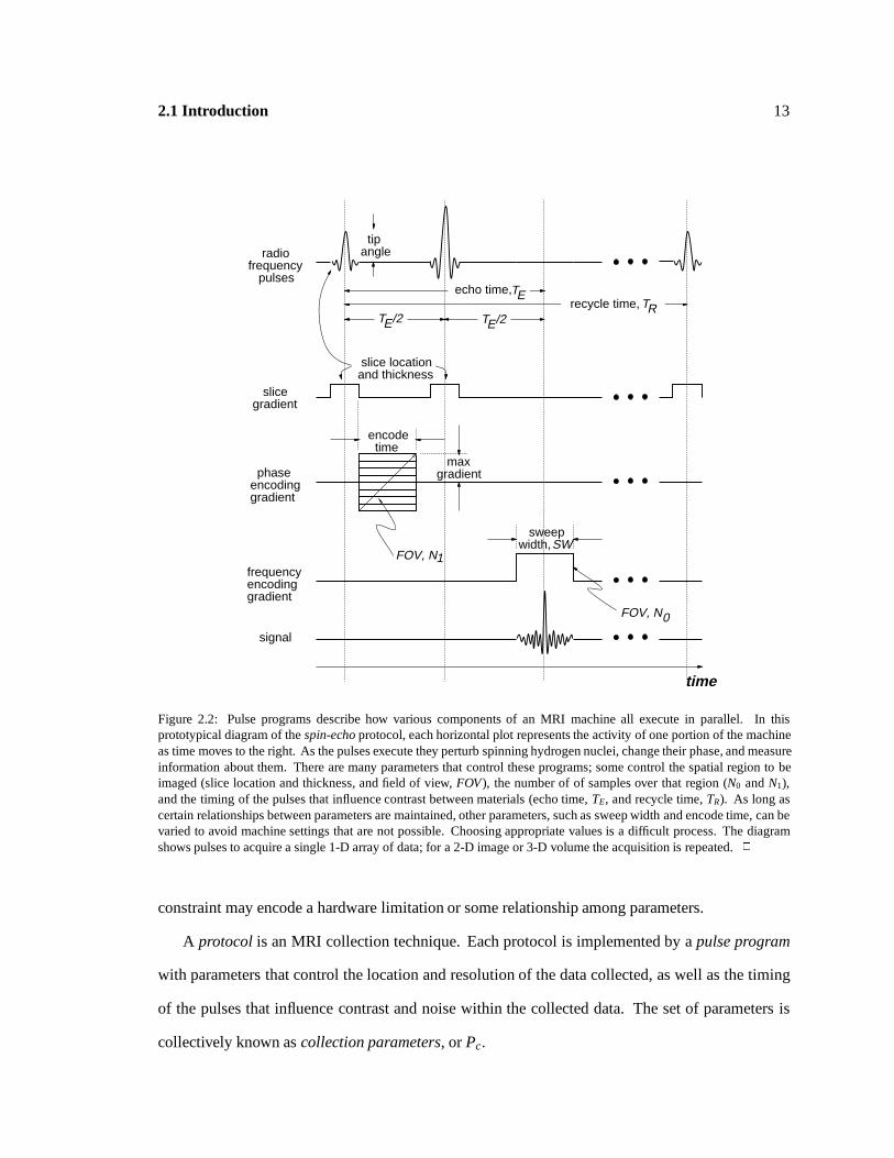
MRI collection protocols are defined by a set of precisely timed electro-magnetic pulses applied
to an object. A “pulse program” defines and controls the exact timing. Figure 2.2 shows an example.
In these programs many operations occur simultaneously: different magnetic gradients are turned
on and off, and radio frequency energy is transmitted into the subject and is measured as it is
re-radiated. The timing of these operations changes the resulting images that are collected, and it is
often difficult to choose appropriate parameter values to collect data that have the properties needed
for a given application.
In most cases finding an appropriate set of parameters is a trial-and-error process. An exper-
imenter typically collects datasets varying the parameters based on prior experience or published
results of other experiments until the images appear reasonably good.
We have improved on this trial-and-error process by mathematically formulating a set of imaging
goals and using constrained optimization to find an optimal set of collection parameters.

2.1 Introduction 12
Collection Parameters, Pc unitsN0;N1;N2 samples none number of samples in each direction–N0 is of-
ten called the read direction; N1, the phase-encode direction; and N2, the slice direction
FOV0,FOV1,FOV2
field of view [m] size of imaged region in each of the abovedirections
H slice thickness [m]Na averages none number of acquisitions averaged together in
each sampleTR recycle time [s] time between acquisitions of data for spins to
realign with the static magnetic fieldTE echo time [s] time within an acquisition for spins to de-phase
due to T2 effectsTI inversion time [s] time within an acquisition for spins to decay
due to T1 effects� tip angle degree angle spins are tipped away from the static
magnetic fieldDW dwell time [s] time to collect a single data point
Table 2.1: The collection parameters in this table control collection protocols, describing the volume to be imaged, thenumber of samples within that volume, and the timing of the pulses that influence contrast between materials. 2
2.1.2 Related Work
Many efforts to find effective MRI collection parameters have centered around finding optimal
contrast between two specific materials, e.g., white matter and grey matter in the human brain
[Dufour et al., 1993]. Other approaches have derived closed-form solutions for optimizing contrast,
contrast-to-noise ratio, or sensitivity [Mitchell et al.,1984] [Fox and Henson, 1986] [Pelc, 1993] [Hendrick
et al., 1984]. Numerical methods have also been employed successfully, most commonly to optimize
the contrast-to-noise ratio, sometimes for a specific collection time [Dreher and Bornert, 1988] [Dufour
et al., 1993] [Epstein et al., 1994].
2.1.3 Terminology
We define terms here that we will use throughout the chapter.
An imaging goal describes a desired property of collected data or of the collection process. An
imaging goal can also be a constraint on a collection parameter or among several parameters. The
2.1 Introduction 13
radiofrequency pulses
slicegradient
phaseencodinggradient
frequencyencodinggradient
signal
sweepwidth,
encode time
tipangle
maxgradient
time
FOV, N0
FOV, N1
echo time,
slice locationand thickness
ETrecycle time, RT
SW
ET /2 ET /2
Figure 2.2: Pulse programs describe how various components of an MRI machine all execute in parallel. In thisprototypical diagram of the spin-echo protocol, each horizontal plot represents the activity of one portion of the machineas time moves to the right. As the pulses execute they perturb spinning hydrogen nuclei, change their phase, and measureinformation about them. There are many parameters that control these programs; some control the spatial region to beimaged (slice location and thickness, and field of view, FOV), the number of of samples over that region (N0 and N1),and the timing of the pulses that influence contrast between materials (echo time, TE, and recycle time, TR). As long ascertain relationships between parameters are maintained, other parameters, such as sweep width and encode time, can bevaried to avoid machine settings that are not possible. Choosing appropriate values is a difficult process. The diagramshows pulses to acquire a single 1-D array of data; for a 2-D image or 3-D volume the acquisition is repeated. 2
constraint may encode a hardware limitation or some relationship among parameters.
A protocol is an MRI collection technique. Each protocol is implemented by a pulse program
with parameters that control the location and resolution of the data collected, as well as the timing
of the pulses that influence contrast and noise within the collected data. The set of parameters is
collectively known as collection parameters, or Pc.

2.2 Conceptual Approach to Goal-Based Data Collection 14
Material Parameters, Pm unitsN(1H) spin density [m�3] number of hydrogen nuclei per volumeT1 longitudinal re-
laxation time[s] time constant for perturbed spins to return to
alignment with the static magnetic fieldT2 transverse relax-
ation time[s] time constant for a collection of spins to go out
of phase
Table 2.2: The three material parameters describe how a region of uniform material will behave under the influence of anMRI collection protocol. The parameters are based on a model of the behavior known as the Bloch equations [Bloch,1948]. 2
Spin-echo is an example of a protocol with the contrast-related parameters TR, TE, and �.
Table 2.1 lists collection parameters; Figure 2.2 shows a prototypical diagram of a spin-echo pulse
program.
A machine is an instance of an MRI machine. Because different MRI machines have hardware
with different capabilities, imaging goals are sometimes implemented differently for different
machines.
Table 2.2 lists material parameters for a model of the MRI process. Material parameters,
sometimes referred to as Pm, describe how a region of homogeneous material behaves as a pulse
program collects data. The parameters include the density of hydrogen nuclei, N(1H), and two
exponential time-constants, T1 and T2, that describe the behavior of the nuclei. The behavior
is based on the Bloch equations [Bloch, 1948], a set of coupled differential equations describing
the behavior of spinning nuclei in time-dependent magnetic fields. Each material has its own
material parameters. The signature for a material is the expected value and standard deviation of
measurements of that material for a given set of protocol parameters.
In many of our results we list the mean, �, and standard deviation, �, of a normal distribution
with the notation “� � �.”
2.2 Conceptual Approach to Goal-Based Data Collection
Our approach builds on the related numerical optimization work (see Section 2.1.2), but uses a
more general goal-based approach and a set of imaging goals that are applicable to more situations.
2.2 Conceptual Approach to Goal-Based Data Collection 15
Collect Images
Interactive --- Once
Automatic --- Iterated
Choose NewParameters
Guess Parameters
Specify Imaging Goals CollectionParameters
ImagesImaging Goals
Start
Doneok? yes
no
Images
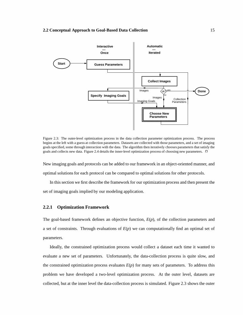
Figure 2.3: The outer-level optimization process in the data collection parameter optimization process. The processbegins at the left with a guess at collection parameters. Datasets are collected with those parameters, and a set of imaginggoals specified, some through interaction with the data. The algorithm then iteratively chooses parameters that satisfy thegoals and collects new data. Figure 2.4 details the inner-level optimization process of choosing new parameters. 2
New imaging goals and protocols can be added to our framework in an object-oriented manner, and
optimal solutions for each protocol can be compared to optimal solutions for other protocols.
In this section we first describe the framework for our optimization process and then present the
set of imaging goals implied by our modeling application.
2.2.1 Optimization Framework
The goal-based framework defines an objective function, E(p), of the collection parameters and
a set of constraints. Through evaluations of E(p) we can computationally find an optimal set of
parameters.
Ideally, the constrained optimization process would collect a dataset each time it wanted to
evaluate a new set of parameters. Unfortunately, the data-collection process is quite slow, and
the constrained optimization process evaluates E(p) for many sets of parameters. To address this
problem we have developed a two-level optimization process. At the outer level, datasets are
collected, but at the inner level the data-collection process is simulated. Figure 2.3 shows the outer

2.2 Conceptual Approach to Goal-Based Data Collection 16
Estimate material parameters
material model
ImagesImagingGoals
Predict material signatures
material signatures
Calculate objective function
objective function
ok?
Select collection parameters
collectionparameters
no
yes
CollectionParameters
Choose
New
Parameters
Figure 2.4: The data collection optimization “inner loop.” This process takes a set of imaging goals and a set of imagesand calculates collection parameters that satisfy the goals. A model for each material is first fit to the set of images, andthen a constrained optimizer iteratively finds the optimal set of protocol parameters based on the material parameters. 2
level. The “Choose New Parameters” step contains the inner level, which is shown in more detail
in Figure 2.4.
In collecting optimized data we perform the steps shown in Figure 2.3. First, we choose an
initial range of collection parameters for the optimization process to use as a starting point. We
collect several datasets with these parameter settings, and then choose geometric locations within
the images that represent different tissues. We then specify a set of imaging goals, e.g.,
� differentiate chosen materials
� acquire data at a particular resolution and size
� minimize collection time
� do not violate hardware limitations of the machine
As shown in Figure 2.4 the constrained optimizer finds an optimal set of parameters based on a
2.2 Conceptual Approach to Goal-Based Data Collection 17
model of each material that we identified in the collected data. New datasets are collected near that
optimal point. Frequently they satisfy the imaging goals, but when they do not, the outer level of
the optimization process is repeated and more new data are collected.
2.2.2 Imaging Goals
We use several different types of imaging goals in our optimization process. Some are related to
the ultimate use of the collected data, some are inferred from constraints of the collection protocol
or machine, and some are practical.
Goal: Good Tissue Discrimination
Our first imaging goal is to be able to unambiguously identify different tissues within an image. The
specific requirements from this goal arise from the tissue-classification algorithms that we present
in Chapters 3–5.
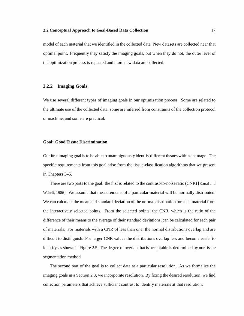
There are two parts to the goal: the first is related to the contrast-to-noise ratio (CNR) [Kanal and
Wehrli, 1986]. We assume that measurements of a particular material will be normally distributed.
We can calculate the mean and standard deviation of the normal distribution for each material from
the interactively selected points. From the selected points, the CNR, which is the ratio of the
difference of their means to the average of their standard deviations, can be calculated for each pair
of materials. For materials with a CNR of less than one, the normal distributions overlap and are
difficult to distinguish. For larger CNR values the distributions overlap less and become easier to
identify, as shown in Figure 2.5. The degree of overlap that is acceptable is determined by our tissue
segmentation method.
The second part of the goal is to collect data at a particular resolution. As we formalize the
imaging goals in a Section 2.3, we incorporate resolution. By fixing the desired resolution, we find
collection parameters that achieve sufficient contrast to identify materials at that resolution.

2.3 Mathematical Approach 18
Pro
babi
lity
Den
sity
MRI Value
Pro
babi
lity
Den
sity
MRI Value
Figure 2.5: On the left two summed normal distributions are difficult to identify, and data values do not clearly lie undereither, making them difficult to assign to a material. On the right the distributions are clearly separated. Note that thisseparation can be achieved either by moving the centers or by narrowing the widths of the distributions. Figures 2.9and 2.10 show examples of data that illustrate this effect. 2
Goal: Observe Machine and Protocol Limitations
We also wish to avoid violating assumptions implied by an imaging protocol or by limitations of
our collection hardware. For example, a given implementation of a spin-echo imaging protocol will
have a maximum value for the parameter TE that is dependent on the value for TR. Similarly, a given
implementation on a particular machine will have a minimum value for TR. The minimum may be
a function of other parameters, or may be an absolute value.
Goal: Minimize Collection Time
We wish to achieve the imaging goals above with the smallest amount of collection time. Imaging
time is expensive, so reducing it saves money. Shorter imaging times also tend to reduce the
likelihood of motion artifacts from living subjects because they do not need to remain in the
machine and motionless for as long.
2.3 Mathematical Approach
In this section we mathematically formulate our imaging goals and the MRI model, describe how we
construct an optimization problem from them, and give some details about the numerical solution

2.3 Mathematical Approach 19
technique that we use.
As shown in Figures 2.3 and 2.4, our algorithm iterates the following steps:
� collect data
� estimate material parameters from data
� optimize collection parameters from MRI model
2.3.1 Model of the MRI Process
The inner loop of our optimization process requires the prediction of material signatures for a given
set of collection parameters. We model the MRI process to do this.
In the model we have chosen [Farrar and Becker, 1971], each material has three parameters, N(1H),
T1, and T2. These parameters are proton spin density, a longitudinal relaxation-time constant and
a transverse relaxation time constant (see Table 2.2). The parameters are defined in the Bloch
equations [Bloch, 1948].
We define three functions that characterize each protocol that we support. We describe them
below. New protocols are added to our framework in an object-oriented manner by specifying these
three functions. The first function, v(Pc;Pm), specifies the data value expected for a given set of
material parameters and collection parameters. The second function, �(Pc;Pm), gives a model of
the standard deviation of the data value as a function of the material and collection parameters.
The third function, t(Pc), defines the collection time necessary to collect data using the collection
parameters.
From data collected with a variety of collection parameters, we estimate the unknown material
parameters for each material, N(1H), T1, and T2, as well as any unknown collection parameters
defined below.
In the estimation procedure we first interactively select locations representing a specific material
within several datasets collected with different collection parameters. For each material in each
dataset, we then calculate the standard deviation of the data values at the selected points and use it
2.3 Mathematical Approach 20
to estimate the measurement error. With the data values and measurement error estimate, we use an
implementation of Levenburg-Marquardt non-linear parameter estimation [Press et al., 1992] to find
the parameters. The parameter-estimation algorithm returns a value, �2, that measures how well
our model fits the data; �2 = 1:0 is a “perfect” fit.
We next describe the equations for several collection protocols. The details of the protocols are
not described here; we need only to know the expected signal, noise, and collection time for a given
set of collection parameters.
Spin-Echo 2-D Protocol
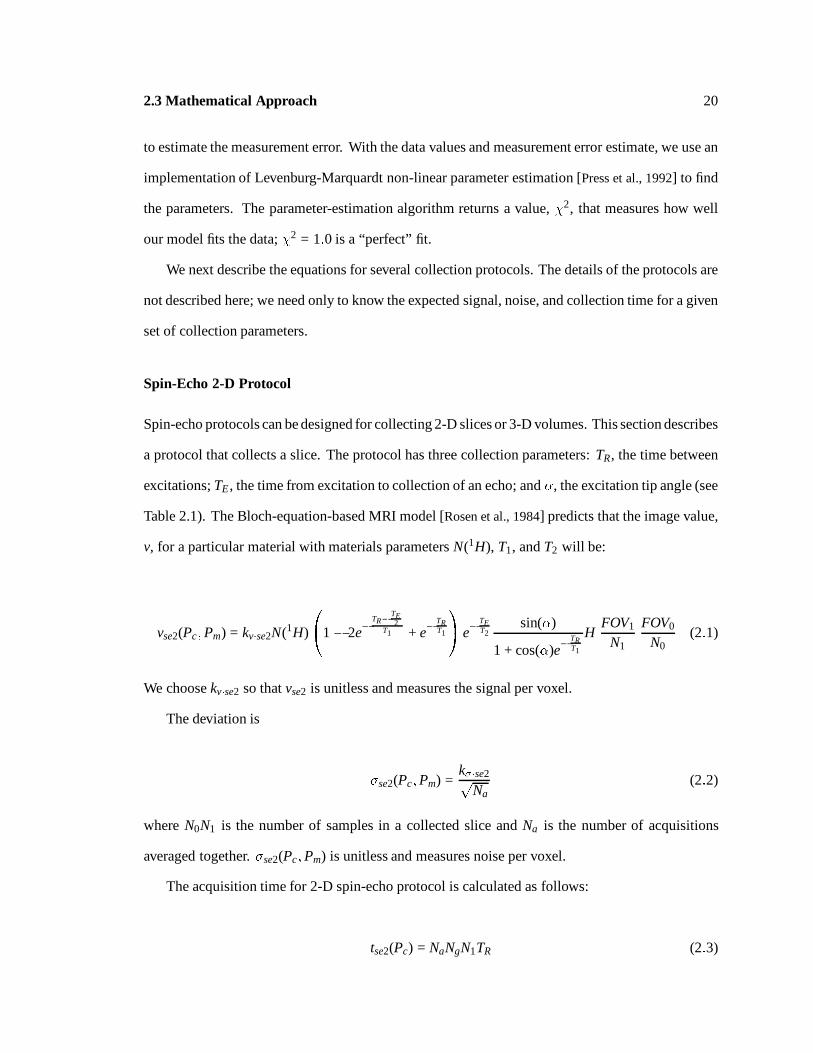
Spin-echo protocols can be designed for collecting 2-D slices or 3-D volumes. This section describes
a protocol that collects a slice. The protocol has three collection parameters: TR, the time between
excitations; TE , the time from excitation to collection of an echo; and �, the excitation tip angle (see
Table 2.1). The Bloch-equation-based MRI model [Rosen et al., 1984] predicts that the image value,
v, for a particular material with materials parameters N(1H), T1, and T2 will be:
vse2(Pc;Pm) = kv�se2N(1H)
0@1� 2e
� TR�TE2
T1 + e� TR
T1
1A e
� TET2
sin(�)
1 + cos(�)e� TR
T1
HFOV1
N1
FOV0
N0(2:1)
We choose kv�se2 so that vse2 is unitless and measures the signal per voxel.
The deviation is
�se2(Pc;Pm) =k��se2p
Na(2:2)
where N0N1 is the number of samples in a collected slice and Na is the number of acquisitions
averaged together. �se2(Pc;Pm) is unitless and measures noise per voxel.
The acquisition time for 2-D spin-echo protocol is calculated as follows:
tse2(Pc) = NaNgN1TR (2:3)
2.3 Mathematical Approach 21
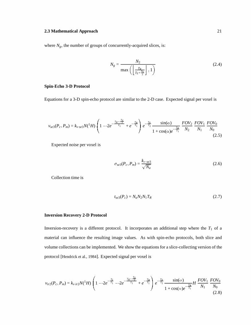
where Ng, the number of groups of concurrently-acquired slices, is:
Ng =N2
max��
TR
TE+N02
�; 1� (2:4)
Spin-Echo 3-D Protocol
Equations for a 3-D spin-echo protocol are similar to the 2-D case. Expected signal per voxel is
vse3(Pc;Pm) = kv�se3N(1H)
0@1� 2e
� TR�TE2
T1 + e� TR
T1
1A e
� TET2
sin(�)
1 + cos(�)e� TR
T1
FOV2
N2
FOV1
N1
FOV0
N0
(2:5)
Expected noise per voxel is
�se3(Pc;Pm) =k��se3p
Na(2:6)
Collection time is
tse3(Pc) = NaN2N1TR (2:7)
Inversion Recovery 2-D Protocol
Inversion-recovery is a different protocol. It incorporates an additional step where the T1 of a
material can influence the resulting image values. As with spin-echo protocols, both slice and
volume collections can be implemented. We show the equations for a slice-collecting version of the
protocol [Hendrick et al., 1984]. Expected signal per voxel is
vir2(Pc;Pm) = kv�ir2N(1H)
0@1� 2e
� TIT1 � 2e
� TR�TE2
T1 + e� TR
T1
1A e
� TET2
sin(�)
1 + cos(�)e� TR
T1
HFOV1
N1
FOV0
N0
(2:8)

2.3 Mathematical Approach 22
Expected noise per voxel is
�ir2(Pc;Pm) =k��ir2p
Na(2:9)
Collection time is
tir2(Pc) = tse2(TR; TE;Na;N2;N1;N0) (2:10)
2.3.2 Imaging Goals
We next describe how our imaging goals are turned into a constrained optimization problem. We
define an objective function, E(p), that we want to minimize subject to a set of constraints, ci. The
constraints are all linear in the parameters that we optimize over, and must be inequalities.
Our objective function is
E(p) =P
I EI(p)
subject to constraints cJ
(2:11)
We decompose each imaging goal into one or more terms, EI(p), in our objective function and
one or more constraints cJ .
Goal: Good Tissue Discrimination
This imaging goal is intended to provide sufficient contrast so that pairs of materials can be
distinguished from one another. For each pair of materials we define a penalty, Edij(p), that is added
to E(p). This penalty is zero where the material data values, vi and vj, are sufficiently separated
relative to their expected deviations, �i and �j.
Edij(p) =max(0; dij(p) � dgij)
kd
2
(2:12)
where dgij is the goal separation between the two materials and dij(p) is that actual separation. kd is
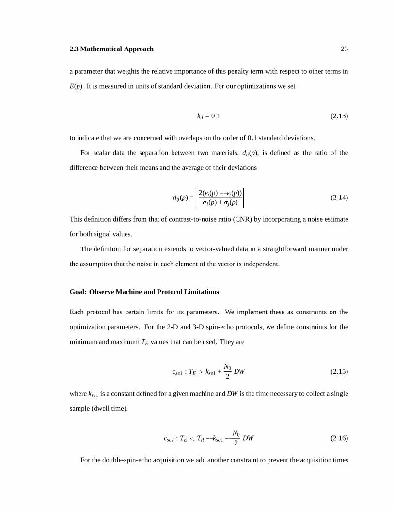
2.3 Mathematical Approach 23
a parameter that weights the relative importance of this penalty term with respect to other terms in
E(p). It is measured in units of standard deviation. For our optimizations we set
kd = 0:1 (2:13)
to indicate that we are concerned with overlaps on the order of 0:1 standard deviations.
For scalar data the separation between two materials, dij(p), is defined as the ratio of the
difference between their means and the average of their deviations
dij(p) =
�����2(vi(p) � vj(p))�i(p) + �j(p)
����� (2:14)
This definition differs from that of contrast-to-noise ratio (CNR) by incorporating a noise estimate
for both signal values.
The definition for separation extends to vector-valued data in a straightforward manner under
the assumption that the noise in each element of the vector is independent.
Goal: Observe Machine and Protocol Limitations
Each protocol has certain limits for its parameters. We implement these as constraints on the
optimization parameters. For the 2-D and 3-D spin-echo protocols, we define constraints for the
minimum and maximum TE values that can be used. They are
cse1 : TE > kse1 +N0
2DW (2:15)
where kse1 is a constant defined for a given machine and DW is the time necessary to collect a single
sample (dwell time).
cse2 : TE < TR � kse2 � N0
2DW (2:16)
For the double-spin-echo acquisition we add another constraint to prevent the acquisition times
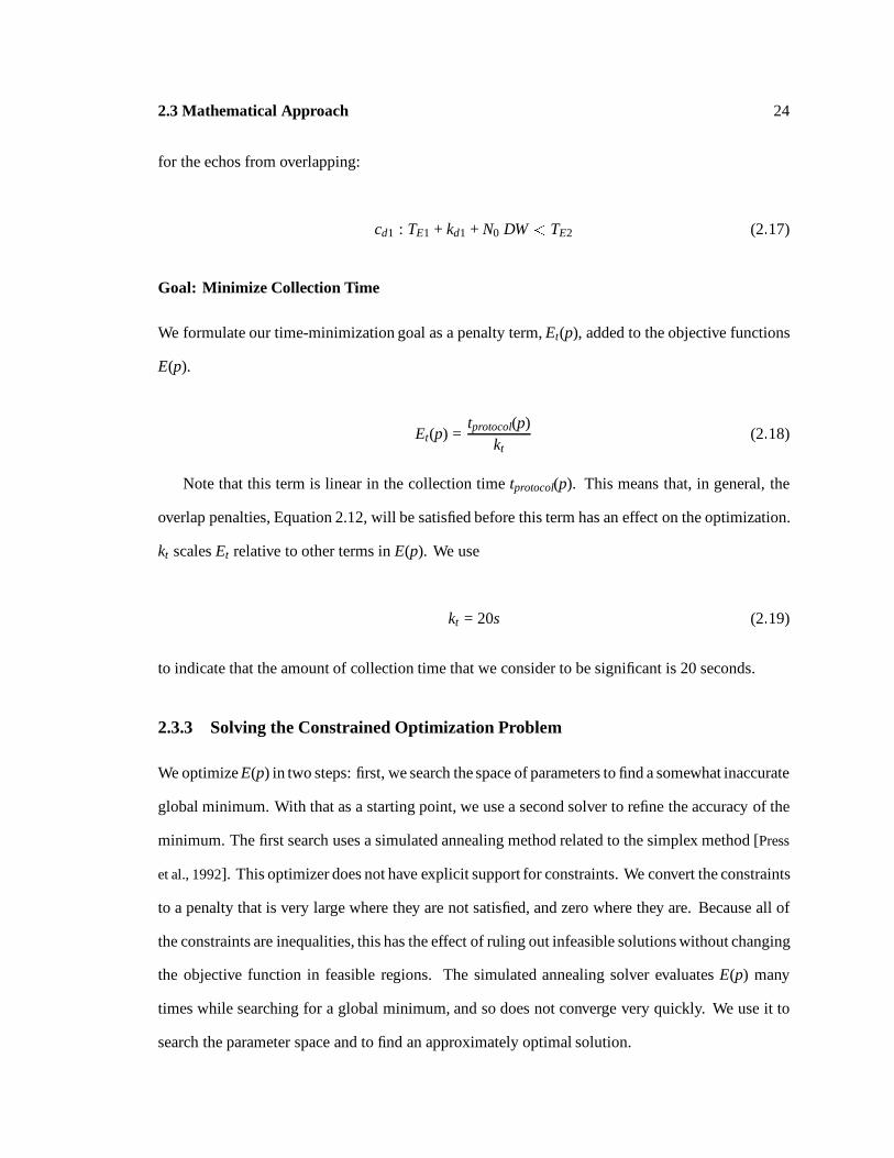
2.3 Mathematical Approach 24
for the echos from overlapping:
cd1 : TE1 + kd1 + N0 DW < TE2 (2:17)
Goal: Minimize Collection Time
We formulate our time-minimization goal as a penalty term, Et(p), added to the objective functions
E(p).
Et(p) =tprotocol(p)
kt(2:18)
Note that this term is linear in the collection time tprotocol(p). This means that, in general, the
overlap penalties, Equation 2.12, will be satisfied before this term has an effect on the optimization.
kt scales Et relative to other terms in E(p). We use
kt = 20s (2:19)
to indicate that the amount of collection time that we consider to be significant is 20 seconds.
2.3.3 Solving the Constrained Optimization Problem
We optimize E(p) in two steps: first, we search the space of parameters to find a somewhat inaccurate
global minimum. With that as a starting point, we use a second solver to refine the accuracy of the
minimum. The first search uses a simulated annealing method related to the simplex method [Press
et al., 1992]. This optimizer does not have explicit support for constraints. We convert the constraints
to a penalty that is very large where they are not satisfied, and zero where they are. Because all of
the constraints are inequalities, this has the effect of ruling out infeasible solutions without changing
the objective function in feasible regions. The simulated annealing solver evaluates E(p) many
times while searching for a global minimum, and so does not converge very quickly. We use it to
search the parameter space and to find an approximately optimal solution.

2.4 Results 25
If there is no feasible solution, the constraints may not be satisfied.
The second optimizer uses a sequential quadratic programming method [NAG, 1993]. It has
very good convergence and explicit support for constraints, but does not search the parameter space
thoroughly, and so would not find the global minimum alone. We start it with the approximate
solution from the first optimizer and it finds a local minimum near its initial solution.
2.4 Results
We tested our methods on simulated data, real data of a Dungeness crab collected in a 1.5 Tesla
clinical machine, and real data of a mouse embryo collected on an 11.7 Tesla research machine.
2.4.1 Simulated Data
We first “collected” simulated data and applied our optimization to it. The “object” that we measured
was a pair of concentric spherical shells, as shown in Figure 2.6. The simulated collection process
used Gaussian sampling to calculate each sample in each dataset based on the geometry, the material
of the “object,” the collection parameters, and Equation 2.1. Normally distributed noise derived
from Equation 2.2 was added to each sample.
Figure 2.7 shows one image for each set of collection parameters used. Table 2.3 shows the
material parameters used and the results of fitting material parameters to the collected data. A �2
of one would indicate that the model has matched the data exactly.
From the estimated material parameters and a set of imaging goals, we estimate collection
parameters that will achieve the goals. Our goals are to achieve a contrast-to-noise ratio of eight
between each of the three pairs of materials and to collect data at the same 10� 40� 40 resolution
at which the calibration data was collected. We chose the resolution and CNR values to collect data
that would work well with our classification algorithms. Figure 2.8 shows two objective functions
for a spin-echo collection. In one Na = 3 and in the other Na = 4. The shape of the objective
function changes for different values of Na with the minimum moving toward smaller TR values on

2.4 Results 26
Figure 2.6: The shape of the object shown in the simulated datasets of Figures 2.7 and 2.9 is two concentric sphericalshells around a hollow interior. The square shows one slice of collected data. 2
TE (ms)
10
16.7
23.3
30
TR (ms)700567433300
Figure 2.7: An array of simulated data “collected” with different TR=TE combinations. All images are displayed on thesame intensity scale, so those with low signal are difficult to see, but still have useful information. The shape of thesimulated object in this figure is shown in Figure 2.6. The brighter region is composed of two materials, although theyare similar and not well differentiated by the collection parameters shown. 2

2.4 Results 27
material parametersmaterial kN(1H) T1 [s] T2 [s] �2
1 3000 1200 120fit 2954� 60 1183� 30 123� 2:5 1.012 3100 1300 100
fit 3269� 72 1379� 37 97:1� 1:4 1.013 0
fit 17:2� 2:1 50:6� 222 122� 87 1.01
Table 2.3: Material parameters for simulated data example. The first row for each material shows the parameters used togenerate the simulated data, and the second row shows the parameters fit to the data, along with a �2 value. A �2 valueof 1.0 indicates that the model fits the data exactly. Values within 0.2 of 1.0 indicate a very good fit. Material 3 has nosignal, so T1 and T2 are not meaningful. 2
10002000
30004000
500050 100 150 200 250
23456789
10
TR
TE (Na = 3)
log(E())
10002000
30004000
500050 100 150 200 250
23456789
10
TR
TE (Na = 4)
log(E())
Figure 2.8: The objective function for the simulated example. We have asked for ten slices at 40x40 resolution, and acontrast-to-noise ratio of eight for each pair of materials. This graph shows two versions of the objective functions for asingle spin-echo acquisition. On the left, Na is fixed at 3, and on the right Na is fixed at 4. The flatter region in the centeris caused by the time minimization goal. It slopes downward toward the origin. The steeper sections are caused by thematerial separation goal. Note that the steep sections are less pronounced with a larger Na because the expected noise inthe dataset is reduced. 2
protocol TR TE Na TR2 TE2 NA2 objective coll. time[ms] [ms] [ms] [ms] [m:s]
spin-echo 1278.9 109.1 4 10.25 3:25spin-echo 1023.5 96.0 5 10.23 3:25
two spin-echos 1308 110.7 4 13.0 8.0 1 10.75 3:34double spin-echo 1276.9 104.3 4 114.3 20.52 6:49
Table 2.4: Optimized collection parameters for simulated data using various protocols. Note the two spin-echos solutionshave almost identical collection times but different collection parameters. Both solutions satisfy the imaging goals of10x10x40 resolution and a contrast-to-noise ratio of eight. For the “two spin-echos” case, two independent spin-echoacquisitions are run sequentially. 2
2.4 Results 28
0
0.001
0.002
0.003
0.004
0.005
0.006
0.007
0 200 400 600 800 1000 1200 1400
Pro
babi
lity
Den
sity
MRI Value (TR/TE = 700/10)
data histogrampredicted material 1 distribution
predicted material 2 distributionpredicted material 3 distribution (air)
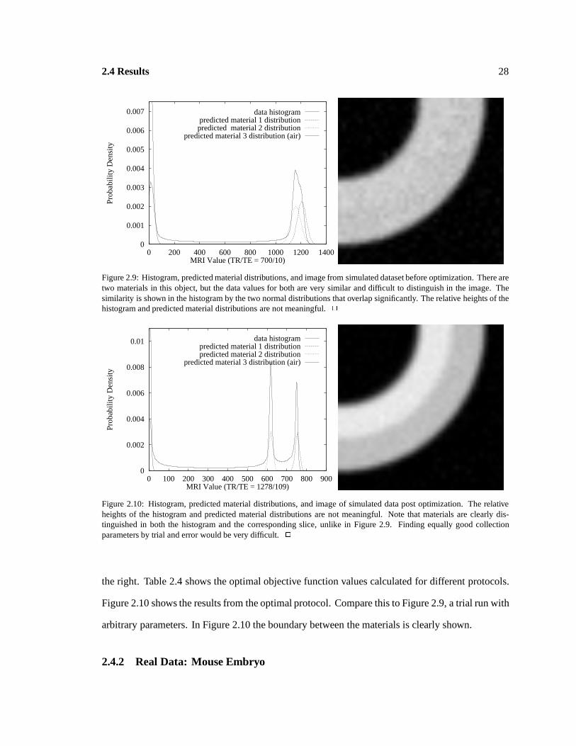
Figure 2.9: Histogram, predicted material distributions, and image from simulated dataset before optimization. There aretwo materials in this object, but the data values for both are very similar and difficult to distinguish in the image. Thesimilarity is shown in the histogram by the two normal distributions that overlap significantly. The relative heights of thehistogram and predicted material distributions are not meaningful. 2
0
0.002
0.004
0.006
0.008
0.01
0 100 200 300 400 500 600 700 800 900
Pro
babi
lity
Den
sity
MRI Value (TR/TE = 1278/109)
data histogrampredicted material 1 distributionpredicted material 2 distribution
predicted material 3 distribution (air)
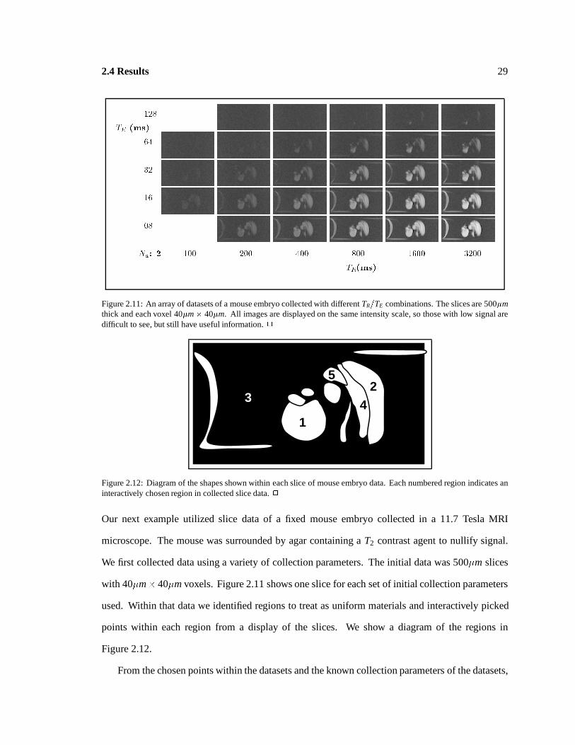
Figure 2.10: Histogram, predicted material distributions, and image of simulated data post optimization. The relativeheights of the histogram and predicted material distributions are not meaningful. Note that materials are clearly dis-tinguished in both the histogram and the corresponding slice, unlike in Figure 2.9. Finding equally good collectionparameters by trial and error would be very difficult. 2
the right. Table 2.4 shows the optimal objective function values calculated for different protocols.
Figure 2.10 shows the results from the optimal protocol. Compare this to Figure 2.9, a trial run with
arbitrary parameters. In Figure 2.10 the boundary between the materials is clearly shown.
2.4.2 Real Data: Mouse Embryo
2.4 Results 29
TE (ms)
08
16
32
64
128
TR(ms)
32001600800400200100Na: 2
Figure 2.11: An array of datasets of a mouse embryo collected with different TR=TE combinations. The slices are 500�mthick and each voxel 40�m� 40�m. All images are displayed on the same intensity scale, so those with low signal aredifficult to see, but still have useful information. 2
1
23 4
5
Figure 2.12: Diagram of the shapes shown within each slice of mouse embryo data. Each numbered region indicates aninteractively chosen region in collected slice data. 2
Our next example utilized slice data of a fixed mouse embryo collected in a 11.7 Tesla MRI
microscope. The mouse was surrounded by agar containing a T2 contrast agent to nullify signal.
We first collected data using a variety of collection parameters. The initial data was 500�m slices
with 40�m� 40�m voxels. Figure 2.11 shows one slice for each set of initial collection parameters
used. Within that data we identified regions to treat as uniform materials and interactively picked
points within each region from a display of the slices. We show a diagram of the regions in
Figure 2.12.
From the chosen points within the datasets and the known collection parameters of the datasets,

2.4 Results 30
estimated material parameters initial datamaterial kN(1H) T1 [s] T2 [s] �2
1 3793� 28:6 1999� 25:6 53� 0:4 1.852 3461� 30:6 1369� 20:5 44� 0:5 1.783 45� 1:0 8� 135:6 5728� 11133:1 1.984 2963� 38:7 1507� 28:8 35� 0:3 1.835 3116� 25:2 1374� 19:4 32� 0:3 1.98
estimated material parameters final iteration1 3468� 21:3 1710� 15:0 54� 0:3 3.212 3373� 29:4 1355� 19:1 45� 0:5 2.053 29� 0:5 9� 137:9 100000� 649816029:7 2.524 2685� 34:9 1490� 29:0 38� 0:3 1.985 3072� 23:9 1328� 16:6 32� 0:2 2.05
Table 2.5: Estimated material parameters for mouse embryo data. We show the parameters as estimated from the initialdatasets, and as re-estimated after four steps of the outer level of the optimization process. Each row shows the materialparameters for one region in the phantom. See Figure 2.12 for the regions corresponding to each row. Because material3 has virtually no signal, the T1 and T2 parameters have almost no influence on Equation 2.1 and the fitted values arearbitrary. 2
iter. protocol TR TE Na TR2 TE2 NA2 objective coll. time[ms] [ms] [ms] [ms] [h:m:s]
1 spin-echo 1272.08 7 28 na na na 238.442 1:15:59two spin-echos 14.2555 9.26 2 1272.12 7 28 238.763 1:16:03
2 spin-echo 1317.62 8.28 30 na na na 258.747 1:24:20two spin-echos 1318.64 8.27 30 12 7 2 259.177 1:24:27
3 spin-echo 1524.26 7 30 na na na 310.623 1:37:33two spin-echos 1126.71 7 16 1738.63 7 16 310.715 1:37:48
4 spin-echo 1343.72 9.40 38 na na na 336.161 1:48:56two spin-echos 1344.3 9.39 38 19.483 14.48 2 336.653 1:49:04
Table 2.6: Optimized collection parameters for phantom data using two protocols. 2
we estimated material parameters for each of the materials as outlined in Section 2.3.1. The
estimated material parameters for this example are shown in the top half of Table 2.5. Because
material 3 produces virtually no signal in the datasets we collected, the T1 and T2 values are not
meaningful.
From the estimated material parameters and a set of imaging goals we estimate collection
parameters that achieve the goals. Our collection goals are to achieve a contrast-to-noise ratio of
six between each pair of materials, and to collect data at the same 256 � 128 resolution as the
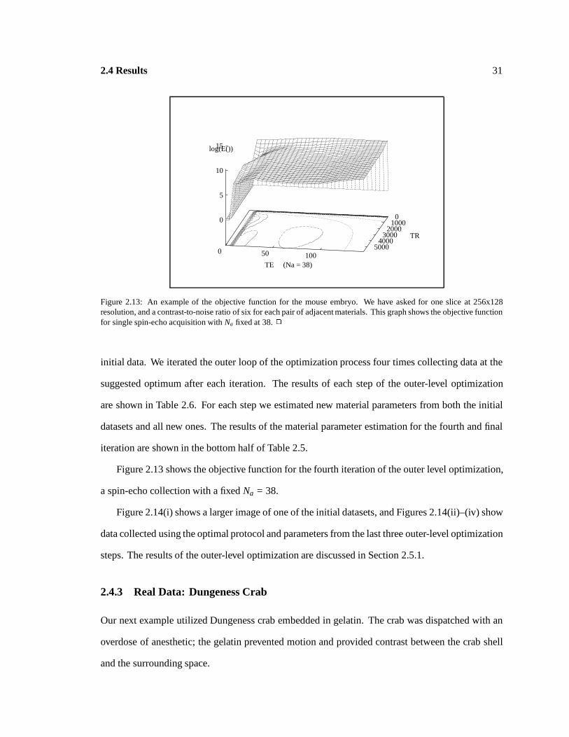
2.4 Results 31
01000
20003000
40005000
0 50 100
0
5
10
15
TR
TE (Na = 38)
log(E())
Figure 2.13: An example of the objective function for the mouse embryo. We have asked for one slice at 256x128resolution, and a contrast-to-noise ratio of six for each pair of adjacent materials. This graph shows the objective functionfor single spin-echo acquisition with Na fixed at 38. 2
initial data. We iterated the outer loop of the optimization process four times collecting data at the
suggested optimum after each iteration. The results of each step of the outer-level optimization
are shown in Table 2.6. For each step we estimated new material parameters from both the initial
datasets and all new ones. The results of the material parameter estimation for the fourth and final
iteration are shown in the bottom half of Table 2.5.
Figure 2.13 shows the objective function for the fourth iteration of the outer level optimization,
a spin-echo collection with a fixed Na = 38.
Figure 2.14(i) shows a larger image of one of the initial datasets, and Figures 2.14(ii)–(iv) show
data collected using the optimal protocol and parameters from the last three outer-level optimization
steps. The results of the outer-level optimization are discussed in Section 2.5.1.
2.4.3 Real Data: Dungeness Crab
Our next example utilized Dungeness crab embedded in gelatin. The crab was dispatched with an
overdose of anesthetic; the gelatin prevented motion and provided contrast between the crab shell
and the surrounding space.
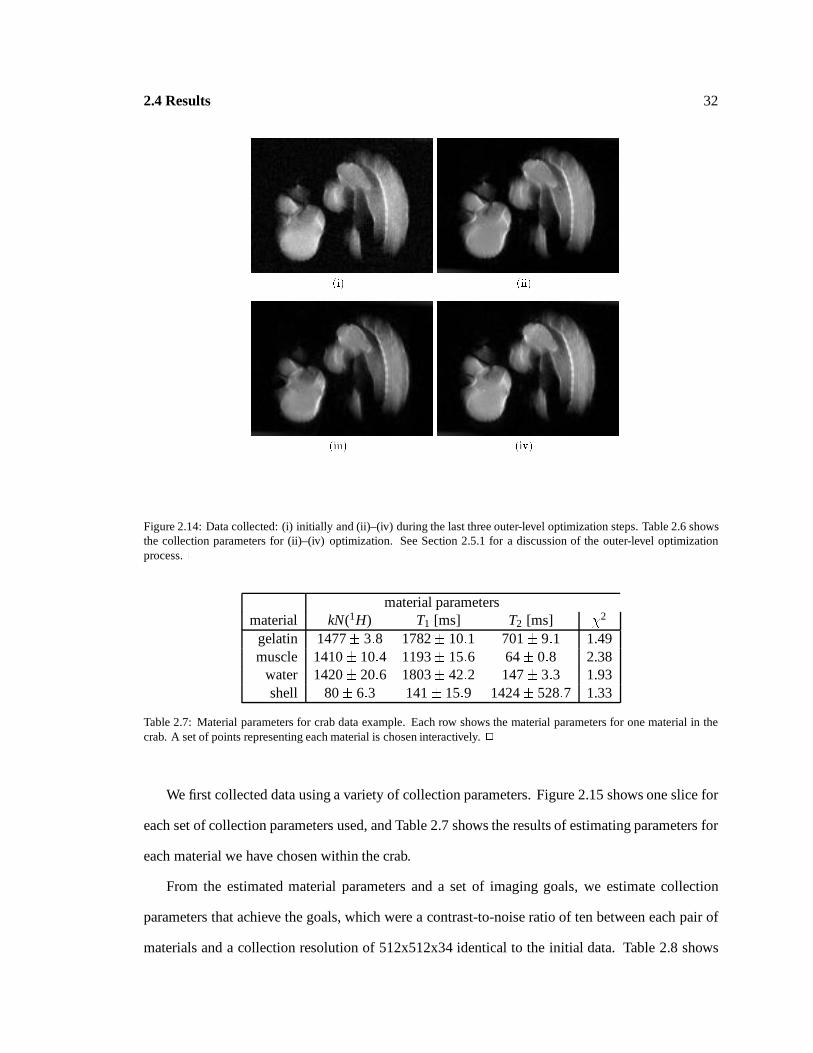
2.4 Results 32
(i) (ii)
(iii) (iv)
Figure 2.14: Data collected: (i) initially and (ii)–(iv) during the last three outer-level optimization steps. Table 2.6 showsthe collection parameters for (ii)–(iv) optimization. See Section 2.5.1 for a discussion of the outer-level optimizationprocess. 2
material parametersmaterial kN(1H) T1 [ms] T2 [ms] �2
gelatin 1477� 3:8 1782� 10:1 701� 9:1 1.49muscle 1410� 10:4 1193� 15:6 64� 0:8 2.38
water 1420� 20:6 1803� 42:2 147� 3:3 1.93shell 80� 6:3 141� 15:9 1424� 528:7 1.33
Table 2.7: Material parameters for crab data example. Each row shows the material parameters for one material in thecrab. A set of points representing each material is chosen interactively. 2
We first collected data using a variety of collection parameters. Figure 2.15 shows one slice for
each set of collection parameters used, and Table 2.7 shows the results of estimating parameters for
each material we have chosen within the crab.
From the estimated material parameters and a set of imaging goals, we estimate collection
parameters that achieve the goals, which were a contrast-to-noise ratio of ten between each pair of
materials and a collection resolution of 512x512x34 identical to the initial data. Table 2.8 shows
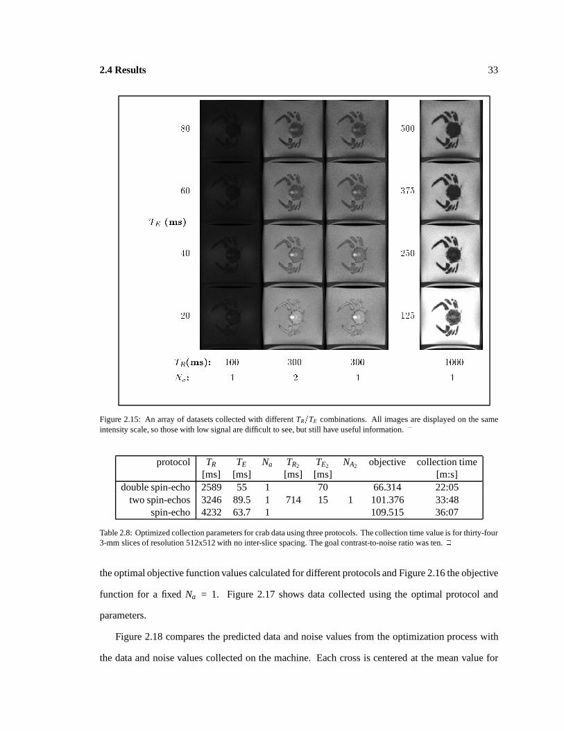
2.4 Results 33
TE (ms)
20
40
60
80
125
250
375
500
TR(ms): 1000300300100
Na: 1121
Figure 2.15: An array of datasets collected with different TR=TE combinations. All images are displayed on the sameintensity scale, so those with low signal are difficult to see, but still have useful information. 2
protocol TR TE Na TR2 TE2 NA2 objective collection time[ms] [ms] [ms] [ms] [m:s]
double spin-echo 2589 55 1 70 66.314 22:05two spin-echos 3246 89.5 1 714 15 1 101.376 33:48
spin-echo 4232 63.7 1 109.515 36:07
Table 2.8: Optimized collection parameters for crab data using three protocols. The collection time value is for thirty-four3-mm slices of resolution 512x512 with no inter-slice spacing. The goal contrast-to-noise ratio was ten. 2
the optimal objective function values calculated for different protocols and Figure 2.16 the objective
function for a fixed Na = 1. Figure 2.17 shows data collected using the optimal protocol and
parameters.
Figure 2.18 compares the predicted data and noise values from the optimization process with
the data and noise values collected on the machine. Each cross is centered at the mean value for
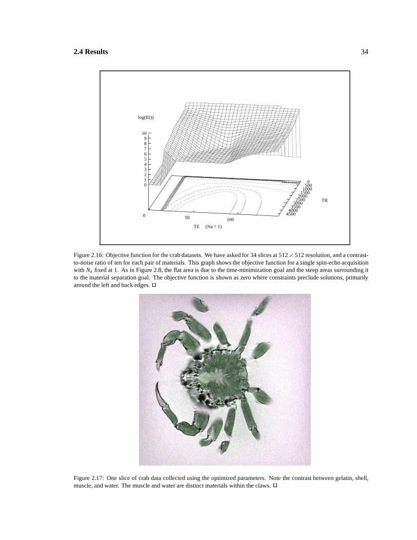
2.4 Results 34
0500
10001500
20002500
30003500
400045000 50 100
0123456789
10
TR
TE (Na = 1)
log(E())
Figure 2.16: Objective function for the crab datasets. We have asked for 34 slices at 512� 512 resolution, and a contrast-to-noise ratio of ten for each pair of materials. This graph shows the objective function for a single spin-echo acquisitionwith Na fixed at 1. As in Figure 2.8, the flat area is due to the time-minimization goal and the steep areas surrounding itto the material separation goal. The objective function is shown as zero where constraints preclude solutions, primarilyaround the left and back edges. 2
Figure 2.17: One slice of crab data collected using the optimized parameters. Note the contrast between gelatin, shell,muscle, and water. The muscle and water are distinct materials within the claws. 2
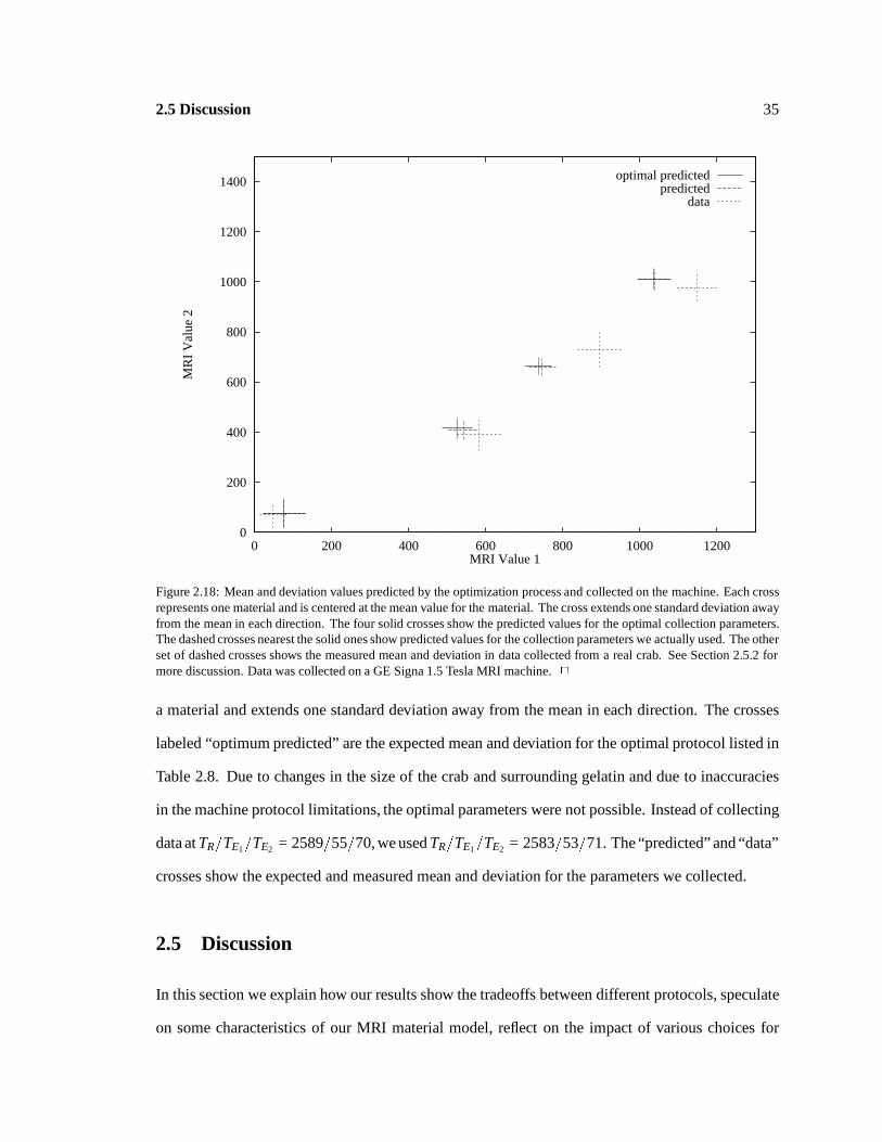
2.5 Discussion 35
0
200
400
600
800
1000
1200
1400
0 200 400 600 800 1000 1200
MR
I V
alue
2
MRI Value 1
optimal predictedpredicted
data
Figure 2.18: Mean and deviation values predicted by the optimization process and collected on the machine. Each crossrepresents one material and is centered at the mean value for the material. The cross extends one standard deviation awayfrom the mean in each direction. The four solid crosses show the predicted values for the optimal collection parameters.The dashed crosses nearest the solid ones show predicted values for the collection parameters we actually used. The otherset of dashed crosses shows the measured mean and deviation in data collected from a real crab. See Section 2.5.2 formore discussion. Data was collected on a GE Signa 1.5 Tesla MRI machine. 2
a material and extends one standard deviation away from the mean in each direction. The crosses
labeled “optimum predicted” are the expected mean and deviation for the optimal protocol listed in
Table 2.8. Due to changes in the size of the crab and surrounding gelatin and due to inaccuracies
in the machine protocol limitations, the optimal parameters were not possible. Instead of collecting
data at TR=TE1=TE2 = 2589=55=70, we used TR=TE1=TE2 = 2583=53=71. The “predicted” and “data”
crosses show the expected and measured mean and deviation for the parameters we collected.
2.5 Discussion
In this section we explain how our results show the tradeoffs between different protocols, speculate
on some characteristics of our MRI material model, reflect on the impact of various choices for
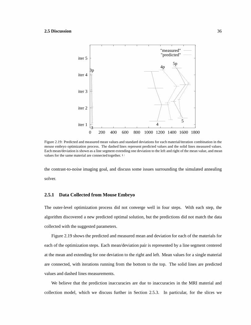
2.5 Discussion 36
iter 1
iter 2
iter 3
iter 4
iter 5
0 200 400 600 800 1000 1200 1400 1600 18003
3p
4
4p
5
5p
"measured""predicted"
Figure 2.19: Predicted and measured mean values and standard deviations for each material/iteration combination in themouse embryo optimization process. The dashed lines represent predicted values and the solid lines measured values.Each mean/deviation is shown as a line segment extending one deviation to the left and right of the mean value, and meanvalues for the same material are connected together. 2
the contrast-to-noise imaging goal, and discuss some issues surrounding the simulated annealing
solver.
2.5.1 Data Collected from Mouse Embryo
The outer-level optimization process did not converge well in four steps. With each step, the
algorithm discovered a new predicted optimal solution, but the predictions did not match the data
collected with the suggested parameters.
Figure 2.19 shows the predicted and measured mean and deviation for each of the materials for
each of the optimization steps. Each mean/deviation pair is represented by a line segment centered
at the mean and extending for one deviation to the right and left. Mean values for a single material
are connected, with iterations running from the bottom to the top. The solid lines are predicted
values and dashed lines measurements.
We believe that the prediction inaccuracies are due to inaccuracies in the MRI material and
collection model, which we discuss further in Section 2.5.3. In particular, for the slices we

2.5 Discussion 37
collected, the slice thickness was over ten times larger than the other voxel dimensions, and so
voxels containing a pure material were difficult to find.
2.5.2 Data Collected from Dungeness Crab
We collected data from one crab and used it to optimize parameters for another. The signal and noise
values in the datasets from the second crab did not exactly match the predicted values generated
using the datasets from the first crab. There are a number of possible explanations for this. First,
the sample was different, although the species in both cases were the same and the preparation
as similar as possible. Second, in addition to regular calibration changes, the MRI machine was
serviced between the initial and final collections, and parts of the gradient amplifiers were replaced.
Third, the temperature of the sample was different between the initial collections and the final
collection. Any of these changes could have affected the data values.
A solution to this problem is to collect initial data, run the optimization while the sample
remains in the machine, and then immediately collect optimized data. The reduced lag time has the
advantage of providing immediate improvement to the collection process and avoiding any changes
that are likely to impact the results. The time to run the optimization is only a few minutes with the
current implementation, and could be sped up significantly.
Our MRI material and collection model also impacts the accuracy of the predictions. See
Section 2.5.3 for more detail.
2.5.3 MRI Material and Collection Model
For a model that matches a set of data values with known normally distributed noise, �2 should be
1. Our simulated data, which is generated with the same model used to fit it, has �2 = 1:01 for all
materials. Within the Dungeness crab and mouse embryo datasets, however, �2 ranges from 1:33
to 3:2. A model that does not fit well creates less-accurate predictions, and data collected at the
predicted points will not satisfy our goals.
We speculate on a number of reasons for the large �2 values. First, in materials with very little
2.5 Discussion 38
signal, such as gasses, hard solids, or the agar/contrast-agent combination used around the mouse
embryo, there is virtually no decay of the signal values. The T1 and T2 parameters, therefore,
provide unused degrees of freedom to the fitting process. In addition, because data values in MR
images are magnitudes of complex numbers, the values will not be normally distributed. For values
where the mean is far from zero relative to the standard deviation, the distribution is very close
to normal. When the mean is close to zero relative to the standard deviation, the distribution can
be quite different from a normal distribution. Our current implementation treats the distribution
as normal, and so gets inaccurate estimates for the signal and noise measurements. It should be
possible to identify both of these cases and correct for them in fitting the model and predicting
results.
A second reason for the large �2 values is that each sample value is an integral over a region
of space. The value incorporates effects from each material within that region, and may not be
representable with a single N(1H); T1, and T2 value. This effect can occur in regions where materials
are mixed together at a scale much smaller than a single voxel. It should be possible to identify cases
where this is happening and address them either by choosing points where materials are not mixed
or by fitting multiple parameter sets to each material to take this small-scale mixing into account.
Chapters 3 and 4 illustrated work in classification of voxels containing mixtures of materials, and
this work may be applicable to the material parameter fitting problem as well.
Finally, the MRI model may fit collected data well, and yet not predict data values accurately. In
particular, when predicting values for collection parameters far from the collection parameters used
to estimate material parameters, material signatures are less accurate. Iterating the outer loop of the
optimization procedure to collect data near the predicted optimal point addresses this problem.
2.5.4 Choice of Protocol
We observe from our experiments that optimizations on machines that support a double spin-echo
collection protocol generally achieve the requested imaging goals with a shorter collection time than
either one or two single spin-echo acquisitions. The double spin-echo protocol collects twice the
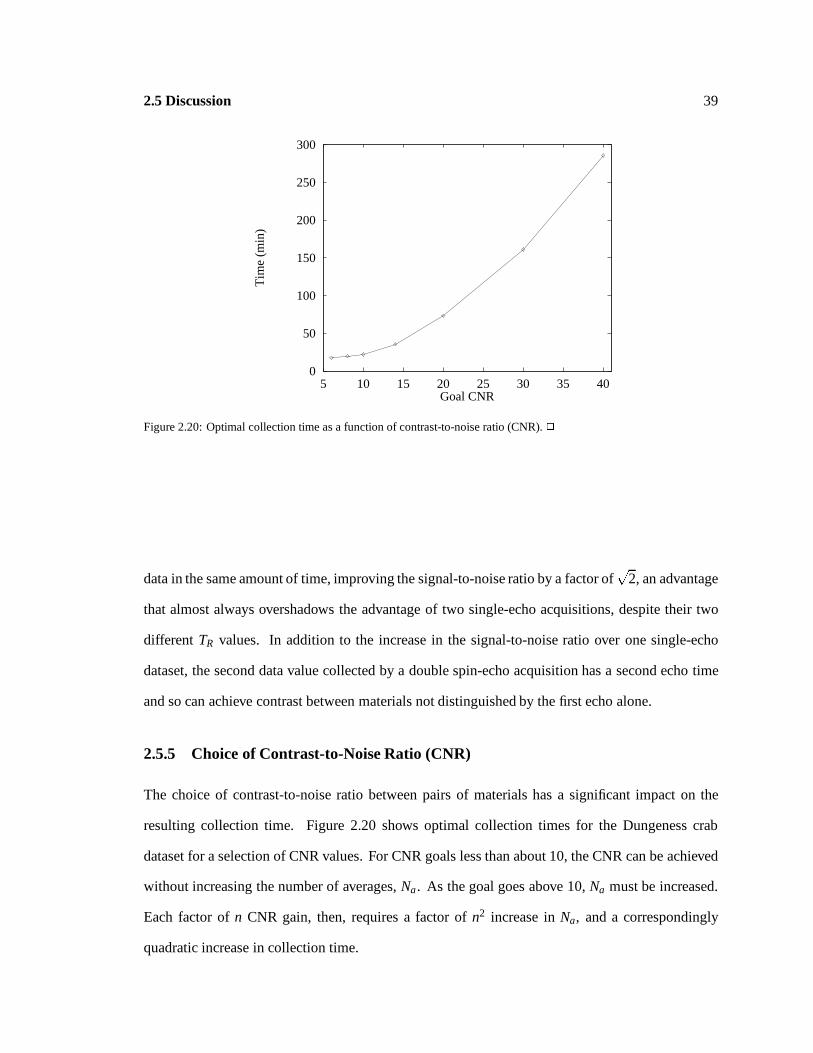
2.5 Discussion 39
0
50
100
150
200
250
300
5 10 15 20 25 30 35 40
Tim
e (m
in)
Goal CNR
Figure 2.20: Optimal collection time as a function of contrast-to-noise ratio (CNR). 2
data in the same amount of time, improving the signal-to-noise ratio by a factor ofp
2, an advantage
that almost always overshadows the advantage of two single-echo acquisitions, despite their two
different TR values. In addition to the increase in the signal-to-noise ratio over one single-echo
dataset, the second data value collected by a double spin-echo acquisition has a second echo time
and so can achieve contrast between materials not distinguished by the first echo alone.
2.5.5 Choice of Contrast-to-Noise Ratio (CNR)
The choice of contrast-to-noise ratio between pairs of materials has a significant impact on the
resulting collection time. Figure 2.20 shows optimal collection times for the Dungeness crab
dataset for a selection of CNR values. For CNR goals less than about 10, the CNR can be achieved
without increasing the number of averages, Na. As the goal goes above 10, Na must be increased.
Each factor of n CNR gain, then, requires a factor of n2 increase in Na, and a correspondingly
quadratic increase in collection time.
2.5 Discussion 40
2.5.6 Solver
Simulated Annealing. Simulated annealing is essential for finding good solutions to the opti-
mization problem we have constructed. The objective function has multiple local minima, some
comparable in magnitude, and some not. Most non-stochastic solvers will find only a nearby local
minima, which may not be adequate. The objective function can also have discontinuities, particu-
larly for the spin-echo 2-D protocol, where the collection time depends on the number of slices that
can be simultaneously collected during a single TR. Many solvers assume continuity and fail when
that assumption is violated.
Annealing Schedule. We have implemented the annealing schedule suggested in [Press et al.,
1992]. The initial annealing temperature is dependent on the CNR imaging goal that we set because
a higher CNR goal creates higher ridges in the objective function. For a CNR goal, g, the maximum
contribution along a ridge created by the goal is�
g2kd
�2. Taking into account overlapping ridges
and the collection-time component of the objective function, we have used an initial temperature of
5000 for CNR goals up to 10.
The annealing schedule must be sufficiently long to explore the space of possible parameters
to find the optimum. The number of function evaluations depends on the number of parameters a
protocol has. For three parameters (2-D spin-echo), 7000 evaluations have been sufficient; for four
parameters (2-D double spin-echo), 12000; and for six parameters (two 2-D spin-echos), 18000.
Speed. Simulated annealing is slow, but for our problems the algorithm has been fast enough,
requiring on the order of 2–15 minutes on an HP9000/700 workstation to find an optimal solution
among two or three protocols. This is fast enough for an object to remain in a scanner while a new
set of parameters is calculated.
2.6 Conclusion 41
2.6 Conclusion
We have presented a goal-based framework for setting up and solving an optimization problem
to find the best protocol and set of parameters for collecting MRI data. Within this framework
we have shown how to implement imaging goals that encode resolution and contrast-to-noise-ratio
requirements of the resulting data, limitations of the MRI machine and collection protocol, and
other goals such as the desire to minimize collection time. The optimization process is independent
of protocol, and we have incorporated a selection of protocols into our implementation.
We have used our implementation to find an optimal protocol and set of parameters for samples
in two MRI machines, as well as for simulated data. The results indicate that an accurate model of
the MRI process improves the accuracy of the optimization process and support our hypothesis that
constrained optimization can be used to select good MRI collection protocols and parameters.
42
PART II
Bayesian Tissue Classification
The following three chapters describe a Bayesian framework for classifying
MRI data and two algorithms developed within the framework. Chapter 3 gives
an introduction to the problem, describes a new Bayesian frameworkfor creating
algorithms to solve the problem, and summarizes a family of new algorithms
we have created within the framework. The algorithms are described in detail
in Chapters 4 and 5.
43
Chapter 3
Bayesian Tissue-Classification Framework
Material classification is a key step in creating computer graphics models and images from vol-
ume data (see Figure 3.1). We present a new Bayesian framework for constructing classification
algorithms and several new algorithms constructed within the framework.
The new algorithms identify the distribution of different material types in volume data such
as those produced with Magnetic Resonance Imaging (MRI) or Computed Tomography (CT). We
apply them to MRI data because MRI measures spatial information about the chemical structure
of an object. Our algorithms treat a voxel as a volume, not as a single point. We reconstruct a
continuous function from the sampled data and use all of the values within each voxel volume to
identify materials within the voxel using a probabilistic approach. The algorithms further assume
that voxels can contain more than one material, e.g., muscle, fat and bone; we compute the relative
quantity of the constituent materials within each voxel.
Other classification methods, as discussed in Section 3.1.1, have utilized Gaussian probability
density functions to model the distribution of values within a dataset. Gaussian basis functions work
well for voxels containing unmixed materials. They do not work well where the materials are mixed

Chapter 3. Bayesian Tissue-Classification Framework 44
Real World Objects
Sampled Volume Data (MR, CT)
Identi�ed Materials
Geometric/Dynamic Models Images/Animation
Data Collection
Classi�cation
ModelBuilding
Volume Rendering/
Visualization
??
??
@@@R
@@@R
���
���
Figure 3.1: Our computational framework for creating geometric models, as shown earlier in Figure 1.1. In Chapters 3–5we describe the classification step, emphasized in the diagram. Our new techniques identify materials in sampled volumedata to produce a new sampled volume dataset for each material. 2
together because measurements combine characteristics of their component materials and are not
normally distributed. We extend the approach by deriving non-Gaussian “mixture” basis functions.
Because we model mixtures of materials and treat voxels as volumes, our techniques reduce the
classification artifacts that occur along boundaries between materials. The techniques are useful for
making higher quality geometric models and renderings from volume data, and have the potential
to make calculations of tissue volumes within a dataset more accurate. They also classify noisy,
low-resolution data well.
3.1 Introduction 45
3.1 Introduction
We begin by describing related work and defining terms. We then present the Bayesian framework
we have developed to create classification algorithms and work through a simple example to illustrate
the process. Section 3.3 gives an overview of the family of new algorithms that we have developed,
deferring their detailed descriptions to Chapters 4 and 5.
3.1.1 Related Work
Much previous work is devoted to material classification in sampled datasets such as those produced
by MRI or CT [Duda and Hart, 1973]. [Clarke et al., 1995] presents a review of classification methods
applied to MRI data. Many of the techniques introduce classification artifacts, particularly on
boundaries between different materials. The artifacts, which tend to appear as jaggy stair steps or
as additional surfaces, are particularly detrimental to computer graphics images and models.
Discrete statistical classification techniques are often used to identify a single class for each
sample within a dataset [Vannier et al., 1985], [Vannier et al., 1988], [Cline et al., 1990]. Each class
contains samples representing a particular material. These techniques work well in regions where
only one material is present, as in the interiors of single-material regions, but tend to fail where
voxels contain boundaries between regions, since a given sample does not represent a single material
there (see Figure 4.1).
[Choi et al., 1991] presents a method that models each sample as representing a mixture of
materials. The technique, like many others, classifies a region based on a single measurement
within the region, effectively treating each voxel as a single point.
3.1.2 Definitions
We refer to the coordinate system of the space of the object we are measuring as spatial coordinates
and generally use x 2 X to refer to points. X is nx-dimensional, where nx is 3 for volume data, but
can be 2 for slices.
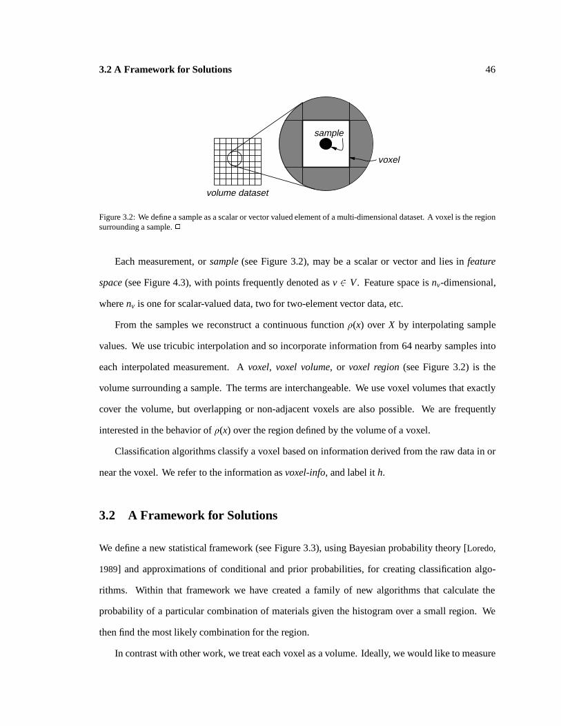
3.2 A Framework for Solutions 46
sample
voxel
volume dataset
Figure 3.2: We define a sample as a scalar or vector valued element of a multi-dimensional dataset. A voxel is the regionsurrounding a sample. 2
Each measurement, or sample (see Figure 3.2), may be a scalar or vector and lies in feature
space (see Figure 4.3), with points frequently denoted as v 2 V . Feature space is nv-dimensional,
where nv is one for scalar-valued data, two for two-element vector data, etc.
From the samples we reconstruct a continuous function �(x) over X by interpolating sample
values. We use tricubic interpolation and so incorporate information from 64 nearby samples into
each interpolated measurement. A voxel, voxel volume, or voxel region (see Figure 3.2) is the
volume surrounding a sample. The terms are interchangeable. We use voxel volumes that exactly
cover the volume, but overlapping or non-adjacent voxels are also possible. We are frequently
interested in the behavior of �(x) over the region defined by the volume of a voxel.
Classification algorithms classify a voxel based on information derived from the raw data in or
near the voxel. We refer to the information as voxel-info, and label it h.
3.2 A Framework for Solutions
We define a new statistical framework (see Figure 3.3), using Bayesian probability theory [Loredo,
1989] and approximations of conditional and prior probabilities, for creating classification algo-
rithms. Within that framework we have created a family of new algorithms that calculate the
probability of a particular combination of materials given the histogram over a small region. We
then find the most likely combination for the region.
In contrast with other work, we treat each voxel as a volume. Ideally, we would like to measure
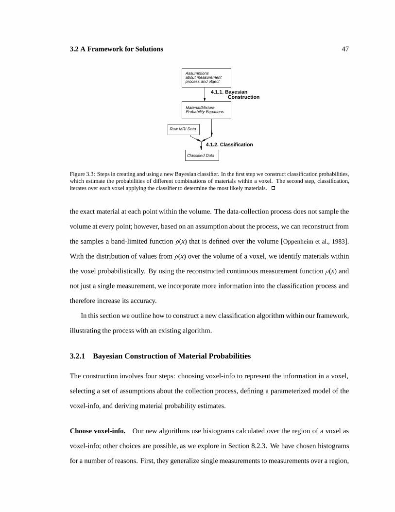
3.2 A Framework for Solutions 47
4.1.1. Bayesian Construction
4.1.2. Classification
Raw MRI Data
Material/MixtureProbability Equations
Classified Data
Assumptionsabout measurementprocess and object
Figure 3.3: Steps in creating and using a new Bayesian classifier. In the first step we construct classification probabilities,which estimate the probabilities of different combinations of materials within a voxel. The second step, classification,iterates over each voxel applying the classifier to determine the most likely materials. 2
the exact material at each point within the volume. The data-collection process does not sample the
volume at every point; however, based on an assumption about the process, we can reconstruct from
the samples a band-limited function �(x) that is defined over the volume [Oppenheim et al., 1983].
With the distribution of values from �(x) over the volume of a voxel, we identify materials within
the voxel probabilistically. By using the reconstructed continuous measurement function �(x) and
not just a single measurement, we incorporate more information into the classification process and
therefore increase its accuracy.
In this section we outline how to construct a new classification algorithm within our framework,
illustrating the process with an existing algorithm.
3.2.1 Bayesian Construction of Material Probabilities
The construction involves four steps: choosing voxel-info to represent the information in a voxel,
selecting a set of assumptions about the collection process, defining a parameterized model of the
voxel-info, and deriving material probability estimates.
Choose voxel-info. Our new algorithms use histograms calculated over the region of a voxel as
voxel-info; other choices are possible, as we explore in Section 8.2.3. We have chosen histograms
for a number of reasons. First, they generalize single measurements to measurements over a region,
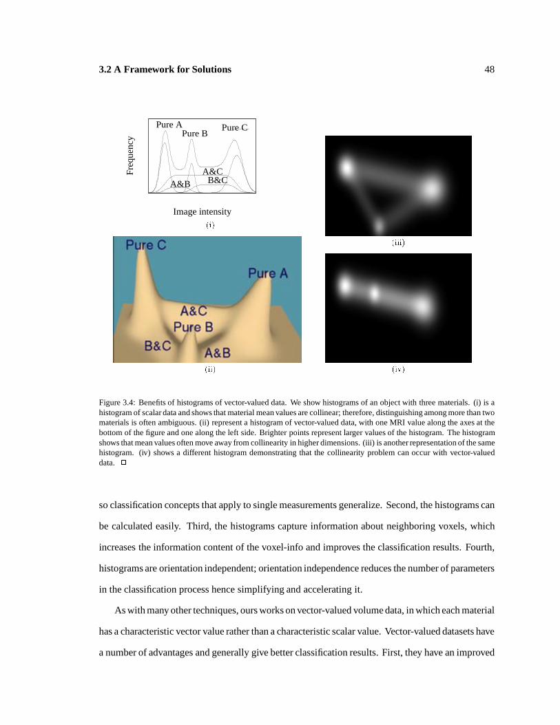
3.2 A Framework for Solutions 48
Freq
uenc
y
Image intensity
Pure APure B
Pure C
A&BA&C
B&C
(i)
(ii)
(iii)
(iv)
Figure 3.4: Benefits of histograms of vector-valued data. We show histograms of an object with three materials. (i) is ahistogram of scalar data and shows that material mean values are collinear; therefore, distinguishing among more than twomaterials is often ambiguous. (ii) represent a histogram of vector-valued data, with one MRI value along the axes at thebottom of the figure and one along the left side. Brighter points represent larger values of the histogram. The histogramshows that mean values often move away from collinearity in higher dimensions. (iii) is another representation of the samehistogram. (iv) shows a different histogram demonstrating that the collinearity problem can occur with vector-valueddata. 2
so classification concepts that apply to single measurements generalize. Second, the histograms can
be calculated easily. Third, the histograms capture information about neighboring voxels, which
increases the information content of the voxel-info and improves the classification results. Fourth,
histograms are orientation independent; orientation independence reduces the number of parameters
in the classification process hence simplifying and accelerating it.
As with many other techniques, ours works on vector-valued volume data, in which each material
has a characteristic vector value rather than a characteristic scalar value. Vector-valued datasets have
a number of advantages and generally give better classification results. First, they have an improved

3.2 A Framework for Solutions 49
signal-to-noise ratio. Second, they frequently distinguish similar materials more effectively (see
Figure 3.4).
In particular, the jump from scalar to two-element vector data is very important. In scalar-valued
datasets it is difficult to distinguish a mixture of two pure materials with values vA and vB from
a pure material with some intermediate value such as vC = (vA + vB)=2. This is because all three
material values are collinear, as they must be for such a dataset.
With more measurement dimensions in the dataset, collinearity is less frequent for most combi-
nations of three or more materials, although Figure 3.4(iv) illustrates that it can still occur. When it
does occur, classification works as for scalar-valued data.
We assume different scalar-valued datasets are spatially aligned so that we can build vector-
valued datasets from them.
Codify collection assumptions. In the second step we codify a set of assumptions about the
data-collection process. The assumptions embody information about:
� how sampling works on the machine we are using,
� the responses of materials or combinations of materials to the measurement process,
� the spatial uniformity of the measurements, and
� geometric restrictions in our objects.
For our example we will assume that there is a known discrete set of materials, that measurements
for a single material are distributed normally, and that each voxel consists of exactly one material.
Section 3.3 lists the assumptions for our new algorithms, some of which are illustrated in Figures 4.1
and 5.1.
Model voxel-info. From our choice of voxel-info and the set of assumptions about the data-
collection process, we define a parameterized model of the voxel-info, f (�). The parameters for the
voxel-info model are divided into two classes. The first, dataset parameters, consists of those that
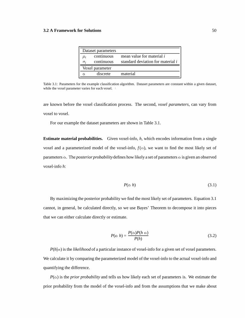
3.2 A Framework for Solutions 50
Dataset parameters�i continuous mean value for material i�i continuous standard deviation for material i
Voxel parameter� discrete material
Table 3.1: Parameters for the example classification algorithm. Dataset parameters are constant within a given dataset,while the voxel parameter varies for each voxel. 2
are known before the voxel classification process. The second, voxel parameters, can vary from
voxel to voxel.
For our example the dataset parameters are shown in Table 3.1.
Estimate material probabilities. Given voxel-info, h, which encodes information from a single
voxel and a parameterized model of the voxel-info, f (�), we want to find the most likely set of
parameters�. The posterior probabilitydefines how likely a set of parameters� is given an observed
voxel-info h:
P(�jh) (3:1)
By maximizing the posterior probability we find the most likely set of parameters. Equation 3.1
cannot, in general, be calculated directly, so we use Bayes’ Theorem to decompose it into pieces
that we can either calculate directly or estimate.
P(�jh) =P(�)P(hj�)
P(h)(3:2)
P(hj�) is the likelihood of a particular instance of voxel-info for a given set of voxel parameters.
We calculate it by comparing the parameterized model of the voxel-info to the actual voxel-info and
quantifying the difference.
P(�) is the prior probability and tells us how likely each set of parameters is. We estimate the
prior probability from the model of the voxel-info and from the assumptions that we make about

3.2 A Framework for Solutions 51
the data-collection process.
P(h) is the global likelihood of a particular instance of voxel-info. We assume that it is a constant
function of h. It becomes a normalization factor for Equation 3.2.
The specific estimates for each of our algorithms are described in subsequent chapters. In the
following section we work through the derivation for an example.
The posterior probability calculation is used within the classifier. For our example, the classifier
calculates the probability of each material for a given measurement and chooses the most likely
material. See Section 4.11 for the detailed derivation of a classifier.
3.2.2 Classification
Estimate dataset parameters. The dataset parameters must be estimated before the classifier
can be used. We estimate them by calculating their values for a training set of voxel-info with
known voxel parameters. In our example we would calculate the mean and variance of a set of
measurements known to be from each discrete material.
Classify voxels. Finally, we calculate the voxel-info for each voxel and use the classifier to
estimate the voxel parameters.
3.2.3 Example of Classification Algorithm Construction
In this section we construct the Bayesian classifier for the example we introduced in Section 3.2.
This classifier is not new [Duda and Hart, 1973], but its construction within our framework illustrates
how to create a classifier.
Example voxel-info. For our example we define voxel-info he as the single data measurement at
the center of a voxel.
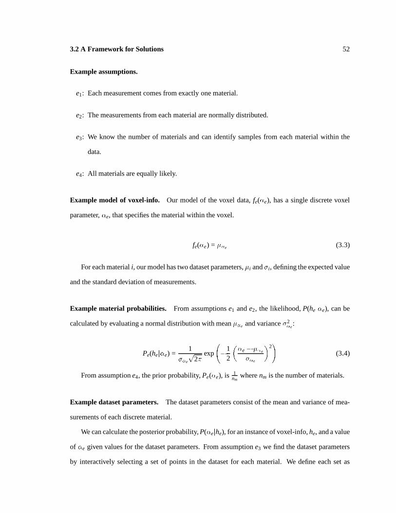
3.2 A Framework for Solutions 52
Example assumptions.
e1: Each measurement comes from exactly one material.
e2: The measurements from each material are normally distributed.
e3: We know the number of materials and can identify samples from each material within the
data.
e4: All materials are equally likely.
Example model of voxel-info. Our model of the voxel data, fe(�e), has a single discrete voxel
parameter, �e, that specifies the material within the voxel.
fe(�e) = ��e (3:3)
For each material i, our model has two dataset parameters, �i and �i, defining the expected value
and the standard deviation of measurements.
Example material probabilities. From assumptions e1 and e2, the likelihood, P(hej�e), can be
calculated by evaluating a normal distribution with mean ��e and variance �2�e
:
Pe(hej�e) =1
��e
p2�
exp
�1
2
��e � ��e
��e
�2!
(3:4)
From assumption e4, the prior probability, Pe(�e), is 1nm
where nm is the number of materials.
Example dataset parameters. The dataset parameters consist of the mean and variance of mea-
surements of each discrete material.
We can calculate the posterior probability, P(�ejhe), for an instance of voxel-info, he, and a value
of �e given values for the dataset parameters. From assumption e3 we find the dataset parameters
by interactively selecting a set of points in the dataset for each material. We define each set as

3.3 A Family of Solutions 53
measurements of the single material they represent; from them we calculate the mean and variance
for each material.
Example classification. We iterate over each voxel calculating the most likely value for the single
voxel parameter �e; for each voxel we measure he, the value at the center of the voxel. For each
possible material we calculate the corresponding posterior probability, P(�ejhe), and choose the
largest of these values. This gives us the most likely material.
3.3 A Family of Solutions
In this section we give an overview of three new classification algorithms constructed within our
framework to compare and contrast them with one another. The algorithms are described in detail
in Chapters 4 and 5. We first list the assumptions that are common to all three algorithms and the
dataset parameters that these assumptions imply. We then present the assumptions unique to each
algorithm and summarize both the dataset and voxel parameters.
3.3.1 Assumptions Common to New Algorithms
We make several assumptions that are consistent among the new algorithms that we have developed.
Each algorithm also makes additional assumptions detailed in Sections 3.3.3–3.3.5.
ec1: Discrete materials. The first assumption is that materials within the objects that we measure
are discrete at the resolution that we are sampling, but not necessarily aligned with the
sampling grid. We make this assumption because we are generally looking for boundaries
between materials, and because we are starting from sampled data, which loses information
about detail that is finer than the sampling rate.
This assumption does not preclude homogeneous combinations of sub-materials that can be
treated as a single material at our sampling resolution. For example, muscle may contain
some water, and yet be treated as a separate material from water. This assumption is not

3.3 A Family of Solutions 54
satisfied where materials gradually transition from one to another over many samples or are
not relatively uniformly mixed. Section 4.8 discusses cases where this assumption is not
satisfied.
ec2: Normally distributed noise. The second assumption is that noise is added to each discrete
sample and that noise is normally distributed. We assume a different variance in the noise for
each material. This assumption is not strictly satisfied for MRI data in some cases, but seems
to be satisfied sufficiently to classify data well.
ec3: Nyquist sampling theorem is satisfied. The third assumption we make is that the sampled
datasets we classify satisfy the Nyquist sampling theorem [Oppenheim et al., 1983]. The
sampling theorem states that if we sample a sufficiently band-limited function, we can exactly
reconstruct that function from the samples.
From assumption ec1 the underlying physical object has discontinuous boundaries between
materials, and an infinite-precision MRI machine would generate a dataset with discontinuities
at material boundaries. At finite resolutions, the measurement function must be band limited
so that it can be reconstructed from the samples.
MRI slice data generally satisfies this assumption or can be pre-processed to satisfy it [Laidlaw,
1992b] within the slice. Without data that satisfy the Nyquist sampling theorem, we cannot
reconstruct a continuous function, and without a continuous function, we cannot extract
geometric models as described in Chapter 6.
3.3.2 Voxel-info: Histograms
For each of our classification techniques we use a histogram over the small region defined by a
voxel to encode the information contained in the voxel. We first reconstruct a continuous function
over the entire dataset from the samples and then use Equation. 4.1 to calculate a histogram over
each voxel.
3.3 A Family of Solutions 55
3.3.3 Overview of Algorithm A: Partial Volume Mixtures
Our new partial volume mixtures algorithm, described in more detail in Chapter 4, was developed
to create classified data with fewer boundary artifacts so that we could produce better geometric
models. The choice of voxel-info, the model of the voxel-info, and some of the assumptions
are formulated to capture and identify information about the boundaries. The remainder of the
assumptions help make some of the probability calculations more tractable.
Additions to common assumptions.
em4: Linear mixtures. Each voxel measurement is a linear combination of pure material mea-
surements and measurements of their pair-wise mixtures.
em5: Uniform tissue measurements. Measurements for the same material have the same expected
value throughout a dataset.
em6: Box filtering. The spatial measurement process can be approximated by a box filter. This
assumption contradicts ec3, but helps us derive a tractable calculation for the histogram basis
function for mixtures which appears to be accurate enough to classify data well.
em7: Materials identifiable in histogram of entire dataset. The signatures for each material and
mixture must be identifiable in a histogram of the entire dataset.
Description. The parameters for each voxel in this algorithm are density values for each pure
material and for each pair-wise combination of materials and an estimate of the low-frequency noise
within the voxel. The densities sum to one, and each density weights a histogram basis function for
either a pure material or a mixture. The basis function for pure materials is a normal distribution.
The basis function for a mixture is derived in Section 4.10. Both are shown in Figure 4.4.
The dataset parameters are the mean and variance values for each pure material, as well as an
expected deviation of the model histogram from actual histograms. The parameters are estimated
3.3 A Family of Solutions 56
by analyzing a histogram taken over the entire dataset and fitting a combination of materials to that
histogram. See Chapter 4 for a complete description.
3.3.4 Overview of Algorithm B: Boundary Distance
Our new boundary distance algorithm, further described in Chapter 5, addresses some of the
limitations we discovered in the partial volume mixtures algorithm. The voxel-info and most of the
assumptions are the same, but the histogram basis functions are new. The main change is that the
distance from a boundary is explicitly incorporated into the histogram basis function for mixtures.
The explicit model better fits histograms of voxels near boundaries. A secondary change is that the
histogram basis functions are derived with the more-accurate assumption of Gaussian filtering.
Addition to common assumptions.
eb4: Only pair-wise mixtures. Each voxel measurement is either a pure material or a mixture of
exactly two materials near a boundary.
eb5: Uniform tissue measurements. Measurements for the same material have the same expected
value throughout a dataset.
eb6: Gaussian filtering. The measurement process can be approximated by a Gaussian filter.
This assumption helps us derive a tractable calculation for the new histogram model of
boundary-parameterized mixtures and also models the actual collection process better than
box filtering.
eb7: Known materials. We know the number of materials and can identify samples from each
material and mixture within the data.
Description. The voxel parameters for this algorithm are a discrete parameter that determines
the material or mixture, a signed distance from a boundary for mixtures, and an estimate of the
low-frequency noise within the voxel. Once again, the histogram basis functions for pure materials
3.3 A Family of Solutions 57
are normal distributions. The basis functions for mixtures are derived in Section 5.8.2 and are shown
in Figures 5.2 and 5.3.
The dataset parameters are the mean and variance values for each pure material, as well as
an expected deviation of the model histogram from actual histograms. They are estimated from
a training set of points interactively chosen for each material and mixture. See Chapter 5 for a
complete description.
3.3.5 Overview of Algorithm C: Boundary Distance with Non-Uniform Material
Signatures
Our third new algorithm, further described in Chapter 5, augments the boundary distance algorithm
to handle a common characteristic of MRI data that often complicates classification: MRI measure-
ments of the same material that are different at different spatial locations. There are a number of
factors that can cause these intensity distortions, from antenna coils that produce spatially dependent
RF radiation to different amounts of absorption of the RF energy in different parts of the object.
The algorithm relaxes the assumption that the expected value for a material is constant. Instead, the
expected value is a function of spatial location.
Additions to common assumptions. Only ev5 differs from the assumptions for the boundary
distance algorithm.
ev4: Only pair-wise mixtures. Each voxel measurement is either a pure material or a mixture of
exactly two materials.
ev5: Predictable tissue measurements. Measurements for the same material have an expected
value that can be modeled with a small number of parameters across a dataset.
ev6: Gaussian filtering. The measurement process can be approximated by a Gaussian filter. This
assumption helps us derive a tractable calculation for the histogram model.
3.4 Summary 58
ev7: Known materials. We know the number of materials and can identify samples from each
material and mixture within the data.
Description. This algorithm is very similar to the boundary distance algorithm. The basis func-
tions and voxel parameters are the same. Only the dataset parameters that determine the expected
value for a tissue measurement are different. In this case, the expected value is a parameterized
function of space. Its parameters are calculated from a set of interactively-specified points for each
material. The calculation is similar to calculating a mean and variance from a set of points, but the
mean is now a function of spatial location.
3.4 Summary
We have presented a Bayesian framework for developing classification algorithms and have outlined
three instances of algorithms. We describe the three algorithms in more detail in the following two
chapters. Chapter 4 discusses the partial volume mixtures algorithm, provides more detail about the
assumptions that it makes, describes the implementation, and presents the results. Chapter 5 does
the same for the two boundary distance algorithms.
59
Chapter 4
Bayesian Classification Algorithm A:
Partial Volume Mixtures
In this chapter we describe a new classification technique. We follow the framework presented in
Chapter 3, first describing the construction of the classification technique and then describing the
implementation that classifies each voxel.
The algorithm uses the probability estimates to classify each voxel in a sampled dataset. The first
step estimates basis-function parameters applicable to the entire dataset. The second step estimates
basis-function parameters for each voxel using the dataset parameters and the probability estimates
and then classifies each voxel based on the estimates.
The input to our process is sampled measurement data, from which we reconstruct a continuous,
band-limited function �(x) that measures distinguishing properties of the underlying materials. Our
unit of voxel-info is a histogram of �(x) taken over a small region. The output is sampled data
measuring the relative volume of each material. We call the output “material volume ratio densities”
(see Figure 4.2).

4.1 Construction 60
A
B
P1
P2
P3
(i)
A
B
A&B
P1
P2
P3
(ii)
Figure 4.1: We start from the assumption that in a real-world object each point is exactly one material, as in (i). Themeasurement process creates samples that mix materials together, from which we reconstruct a continuous, band-limitedmeasurement function �(x). For some values of x, e.g., P1 and P2, �(x) returns the signature of a pure material. For othervalues of x, e.g., P3, �(x) returns a combination of the pure material signatures. (ii) shows regions A and B where �(x)returns pure material signatures and region A&B, where �(x) returns a combination. The grid lines show how the materialregions may span voxels. 2
We assume, as in Figure 4.1, that each voxel is a mixture of materials, with mixtures like A & B
occurring where the band-limiting effects of the data collection process blur pure materials together.
From this assumption we derive basis functions that model histograms for pure materials and for
mixtures of two materials.
We give an overview of the construction of the algorithm in Section 4.1 and of the implementation
in Section 4.2. Sections 4.3 and 4.4 give more details on histograms and the basis functions for
modeling them, and Sections 4.5 and 4.6 describe estimating dataset and voxel parameters. We
present results in Section 4.7 and discuss the results and algorithm in Section 4.8. Detailed
derivations follow in Sections 4.10 and 4.11.
4.1 Construction
The construction of the algorithm starts with a choice of voxel data and a set of assumptions and
proceeds through a derivation of basis functions to match a model to the voxel data. This section
describes the construction process.
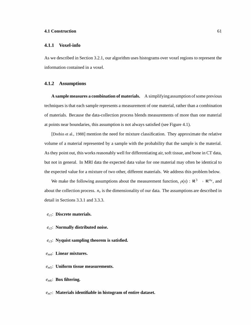
4.1 Construction 61
4.1.1 Voxel-info
As we described in Section 3.2.1, our algorithm uses histograms over voxel regions to represent the
information contained in a voxel.
4.1.2 Assumptions
A sample measures a combination of materials. A simplifyingassumption of some previous
techniques is that each sample represents a measurement of one material, rather than a combination
of materials. Because the data-collection process blends measurements of more than one material
at points near boundaries, this assumption is not always satisfied (see Figure 4.1).
[Drebin et al., 1988] mention the need for mixture classification. They approximate the relative
volume of a material represented by a sample with the probability that the sample is the material.
As they point out, this works reasonably well for differentiating air, soft tissue, and bone in CT data,
but not in general. In MRI data the expected data value for one material may often be identical to
the expected value for a mixture of two other, different materials. We address this problem below.
We make the following assumptions about the measurement function, �(x) : R3 ! Rnv , and
about the collection process. nv is the dimensionality of our data. The assumptions are described in
detail in Sections 3.3.1 and 3.3.3.
ec1: Discrete materials.
ec2: Normally distributed noise.
ec3: Nyquist sampling theorem is satisfied.
em4: Linear mixtures.
em5: Uniform tissue measurements.
em6: Box filtering.
em7: Materials identifiable in histogram of entire dataset.
4.2 Algorithm 62
For many types of medical imaging data, including MRI and CT, these assumptions hold
reasonably well, or can be satisfied sufficiently with preprocessing [Laidlaw, 1992a]. Other types
of sampled data, e.g., ultrasound and sequences of video or film images with lighting and shading,
violate these assumptions, and our technique does not apply directly.
4.1.3 Sketch of Derivation
As shown in Figure 4.1 we start with the assumption that each spatial location in the real world
object is exactly one material, and that the measurement process mixes materials together as it band
limits the measurements to the Nyquist frequency of the sampling rate. From that assumption we
will derive (in Section 4.3) an equation for a normalized histogram of data values within a region.
This histogram function is a probability density function (PDF) that tells us the probability that a
measurement will lie within a range of values in that region.
In Section 4.10 we create basis functions to model histograms. These basis functions are
parameterized probability density functions for regions consisting of single materials and for regions
consisting of mixtures of two materials. These mixtures are assumed to have been created by the
band-limiting process accompanying sampling. The parameters represent the mean value, c, and
variance, s, of a measurement.
Using Bayes’ Theorem, the histogram of the entire dataset, our model basis functions, and a
series of approximations, we derive an estimate of the most likely set of materials within an entire
dataset (Section 4.11). Similarly, given the histogram of a voxel region, we derive an estimate of
the most likely density for each material in that region (Section 4.6).
4.2 Algorithm
The algorithm produces, as its end result, a sampled dataset containing estimates of material volume
ratio densities. The process is illustrated in Figure 4.2.

4.2 Algorithm 63
Volume Ratio Densities
Sampled MR Data
Fitted Histogram
Whole Dataset Histogram, h (v)
Histograms of Voxel-sizedRegions, h (v)
Real World Object
FittedHistograms
all
vox
Figure 4.2: Steps in the classification process. We collect MR data, calculate a histogram of the entire dataset, hall(v), anduse that to determine parameters of histogram-fitting basis functions. We then calculate histograms of each voxel region,hvox(v), and identify the most likely mixture of materials for that region. The result is a sampled dataset of volume ratiodensities. 2
Estimating dataset parameters. First, we collect and preprocess data to satisfy the assumptions
listed above. Second, we calculate a histogram of the entire dataset, and fit parameterized material
probability density functions to the histogram to get an estimate of basis function parameters that
are constant throughout the dataset.
4.3 Normalized Histograms 64
Estimating voxel parameters. Using the fitted parameters, we process the region for each voxel in
the dataset as follows. We first calculate a histogram for the small region and find the combination of
materials most closely fitting the histogram. Using the estimated parameters, we calculate material
volume ratio densities for that small region.
4.3 Normalized Histograms
In this section we present the equation for a normalized histogram of a sampled dataset over a
region. We will use this equation as a building block in several later sections, with regions that
vary from the size of a single voxel to regions covering the entire dataset. We will also use this
equation to derive basis functions that model histograms over regions containing single materials and
regions containing mixtures of materials. Figure 4.3 shows an example of calculating a normalized
histogram from a continuous function.
For a given region in spatial coordinates, specified by R, the histogram hR(v) specifies the
relative portion of that region where �(x) = v. We define histograms, hR(v) : Rnv ! R; as
probability density functions (PDFs). These histograms over regions are also continuous functions:
hR(v) =ZR(x)�(�(x) � v)dx (4:1)
This equation is the continuous analog of a discrete histogram. R(x) is non-zero within the
region of interest, and integrates to 1. We defineR(x) to be constant in the region of interest making
every spatial point contribute equally to the histogram hR(v). Note also that hR(v) integrates to 1,
which is important for our interpretation as a PDF. � is the Dirac-delta function.
We use this equation both as a starting point for deriving material intensity PDFs, and also as
a basis for calculating histograms of regions of our datasets. The derivations are outlined in the
following two sections and detailed in Section 4.10. We will now discuss a few implementation
considerations for calculating histograms.
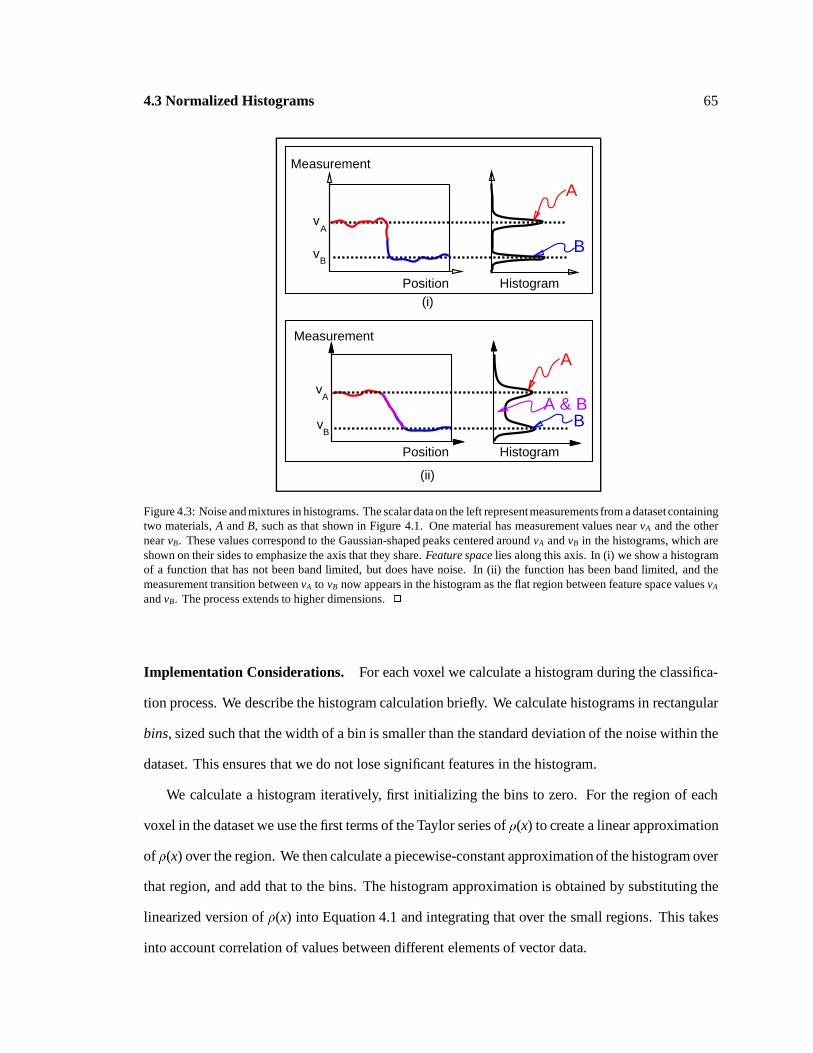
4.3 Normalized Histograms 65
vA
vB
Histogram
Measurement
Histogram
A & B
A
B
A
B
vA
vB
Position
Position
Measurement
(i)
(ii)
Figure 4.3: Noise and mixtures in histograms. The scalar data on the left representmeasurements from a dataset containingtwo materials, A and B, such as that shown in Figure 4.1. One material has measurement values near vA and the othernear vB. These values correspond to the Gaussian-shaped peaks centered around vA and vB in the histograms, which areshown on their sides to emphasize the axis that they share. Feature space lies along this axis. In (i) we show a histogramof a function that has not been band limited, but does have noise. In (ii) the function has been band limited, and themeasurement transition between vA to vB now appears in the histogram as the flat region between feature space values vA
and vB. The process extends to higher dimensions. 2
Implementation Considerations. For each voxel we calculate a histogram during the classifica-
tion process. We describe the histogram calculation briefly. We calculate histograms in rectangular
bins, sized such that the width of a bin is smaller than the standard deviation of the noise within the
dataset. This ensures that we do not lose significant features in the histogram.
We calculate a histogram iteratively, first initializing the bins to zero. For the region of each
voxel in the dataset we use the first terms of the Taylor series of �(x) to create a linear approximation
of �(x) over the region. We then calculate a piecewise-constant approximation of the histogram over
that region, and add that to the bins. The histogram approximation is obtained by substituting the
linearized version of �(x) into Equation 4.1 and integrating that over the small regions. This takes
into account correlation of values between different elements of vector data.
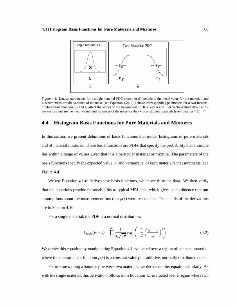
4.4 Histogram Basis Functions for Pure Materials and Mixtures 66
c
s
Single Material PDF Two-Material PDF
c 0 c 1
s1 s0
(i) (ii)
Figure 4.4: Dataset parameters for a single material PDF, shown in (i) include c, the mean value for the material, ands, which measures the variance of the noise (see Equation 4.2). (ii) shows corresponding parameters for a two-materialmixture basis function. s0 and s1 affect the slopes of the two-material PDF at either end. For vector-valued data c and sare vectors and are the mean values and variances of the noise for the two constituent materials (see Equation 4.3). 2
4.4 Histogram Basis Functions for Pure Materials and Mixtures
In this section we present definitions of basis functions that model histograms of pure materials
and of material mixtures. These basis functions are PDFs that specify the probability that a sample
lies within a range of values given that it is a particular material or mixture. The parameters of the
basis functions specify the expected value, c, and variance, s, of each material’s measurements (see
Figure 4.4).
We use Equation 4.1 to derive these basis functions, which we fit to the data. We then verify
that the equations provide reasonable fits to typical MRI data, which gives us confidence that our
assumptions about the measurement function �(x) were reasonable. The details of the derivations
are in Section 4.10.
For a single material, the PDF is a normal distribution:
fsingle(v; c; s) =nvYi=1
1
sip
2�exp
�1
2
�vi � ci
si
�2!
(4:2)
We derive this equation by manipulating Equation 4.1 evaluated over a region of constant material,
where the measurement function �(x) is a constant value plus additive, normally distributed noise.
For mixtures along a boundary between two materials, we derive another equation similarly. As
with the single material, this derivation follows from Equation 4.1 evaluated over a region where two
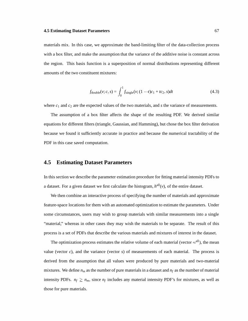
4.5 Estimating Dataset Parameters 67
materials mix. In this case, we approximate the band-limiting filter of the data-collection process
with a box filter, and make the assumption that the variance of the additive noise is constant across
the region. This basis function is a superposition of normal distributions representing different
amounts of the two constituent mixtures:
fdouble(v; c; s) =Z 1
0fsingle(v; (1� t)c1 + tc2; s)dt (4:3)
where c1 and c2 are the expected values of the two materials, and s the variance of measurements.
The assumption of a box filter affects the shape of the resulting PDF. We derived similar
equations for different filters (triangle, Gaussian, and Hamming), but chose the box filter derivation
because we found it sufficiently accurate in practice and because the numerical tractability of the
PDF in this case saved computation.
4.5 Estimating Dataset Parameters
In this section we describe the parameter estimation procedure for fitting material intensity PDFs to
a dataset. For a given dataset we first calculate the histogram, hall(v), of the entire dataset.
We then combine an interactive process of specifying the number of materials and approximate
feature-space locations for them with an automated optimization to estimate the parameters. Under
some circumstances, users may wish to group materials with similar measurements into a single
“material,” whereas in other cases they may wish the materials to be separate. The result of this
process is a set of PDFs that describe the various materials and mixtures of interest in the dataset.
The optimization process estimates the relative volume of each material (vector �all), the mean
value (vector c), and the variance (vector s) of measurements of each material. The process is
derived from the assumption that all values were produced by pure materials and two-material
mixtures. We define nm as the number of pure materials in a dataset and nf as the number of material
intensity PDFs. nf � nm, since nf includes any material intensity PDF’s for mixtures, as well as
those for pure materials.
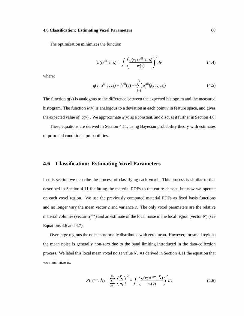
4.6 Classification: Estimating Voxel Parameters 68
The optimization minimizes the function
E(�all; c; s) =Z
q(v;�all; c; s)w(v)
!2
dv (4:4)
where:
q(v;�all; c; s) = hall(v) �nfXj=1
�allj fj(v; cj; sj) (4:5)
The function q(v) is analogous to the difference between the expected histogram and the measured
histogram. The function w(v) is analogous to a deviation at each point v in feature space, and gives
the expected value of jq(v)j. We approximate w(v) as a constant, and discuss it further in Section 4.8.
These equations are derived in Section 4.11, using Bayesian probability theory with estimates
of prior and conditional probabilities.
4.6 Classification: Estimating Voxel Parameters
In this section we describe the process of classifying each voxel. This process is similar to that
described in Section 4.11 for fitting the material PDFs to the entire dataset, but now we operate
on each voxel region. We use the previously computed material PDFs as fixed basis functions
and no longer vary the mean vector c and variance s. The only voxel parameters are the relative
material volumes (vector �voxj ) and an estimate of the local noise in the local region (vector �N) (see
Equations 4.6 and 4.7).
Over large regions the noise is normally distributed with zero mean. However, for small regions
the mean noise is generally non-zero due to the band limiting introduced in the data-collection
process. We label this local mean voxel noise value �N. As derived in Section 4.11 the equation that
we minimize is:
E(�vox; �N) =nvXi=1
� �Ni
�i
�2
+Z �
q(v;�vox; �N)w(v)
�2
dv (4:6)
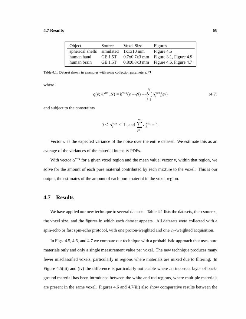
4.7 Results 69
Object Source Voxel Size Figuresspherical shells simulated 1x1x10 mm Figure 4.5human hand GE 1.5T 0.7x0.7x3 mm Figure 3.1, Figure 4.9human brain GE 1.5T 0.8x0.8x3 mm Figure 4.6, Figure 4.7
Table 4.1: Dataset shown in examples with some collection parameters. 2
where
q(v;�vox; �N) = hvox(v� �N)�nfXj=1
�voxj fj(v) (4:7)
and subject to the constraints
0 � �voxj � 1; and
nfXj=1
�voxj = 1:
Vector � is the expected variance of the noise over the entire dataset. We estimate this as an
average of the variances of the material intensity PDFs.
With vector �vox for a given voxel region and the mean value, vector �v, within that region, we
solve for the amount of each pure material contributed by each mixture to the voxel. This is our
output, the estimates of the amount of each pure material in the voxel region.
4.7 Results
We have applied our new technique to several datasets. Table 4.1 lists the datasets, their sources,
the voxel size, and the figures in which each dataset appears. All datasets were collected with a
spin-echo or fast spin-echo protocol, with one proton-weighted and one T2-weighted acquisition.
In Figs. 4.5, 4.6, and 4.7 we compare our technique with a probabilistic approach that uses pure
materials only and only a single measurement value per voxel. The new technique produces many
fewer misclassified voxels, particularly in regions where materials are mixed due to filtering. In
Figure 4.5(iii) and (iv) the difference is particularly noticeable where an incorrect layer of back-
ground material has been introduced between the white and red regions, where multiple materials
are present in the same voxel. Figures 4.6 and 4.7(iii) also show comparative results between the
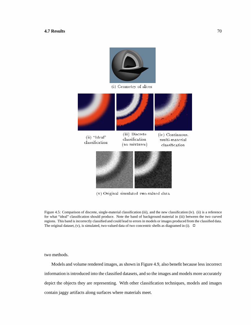
4.7 Results 70
(i) Geometry of slices
(ii) \Ideal"classi�cation
(iii) Discreteclassi�cation(no mixtures)
(iv) Continuous,multi-materialclassi�cation
(v) Original simulated two-valued data
Figure 4.5: Comparison of discrete, single-material classification (iii), and the new classification (iv). (ii) is a referencefor what “ideal” classification should produce. Note the band of background material in (iii) between the two curvedregions. This band is incorrectly classified and could lead to errors in models or images produced from the classified data.The original dataset, (v), is simulated, two-valued data of two concentric shells as diagramed in (i). 2
two methods.
Models and volume rendered images, as shown in Figure 4.9, also benefit because less incorrect
information is introduced into the classified datasets, and so the images and models more accurately
depict the objects they are representing. With other classification techniques, models and images
contain jaggy artifacts along surfaces where materials meet.

4.8 Discussion 71
Figure 4.6: Discrete, single-material classification of the same slice shown in Figure 4.7. 2
Implementation. Our implementation is written in C and C++ on Unix workstations. We use
a sequential quadratic programming constrained optimization algorithm [NAG, 1993] to fit hvox
for each voxel region, and a quasi-Newton optimization algorithm for fitting hall. The algorithm
classifies approximately 10 voxels per second on a single HP9000/730, IBM RS6000/550E, or DEC
Alpha AXP 3000 Model 500 workstation. We have implemented this algorithm in parallel on these
machines, and get a corresponding speedup on multiple machines.
4.8 Discussion
We have made several assumptions and approximations while developing and implementing this
algorithm. This section will discuss some of the tradeoffs and suggest some possible directions for
future work.
Mixtures of Three or More Materials. We assume that each measurement contains values
from at most two materials, although our approach easily extends to mixtures with more materials.
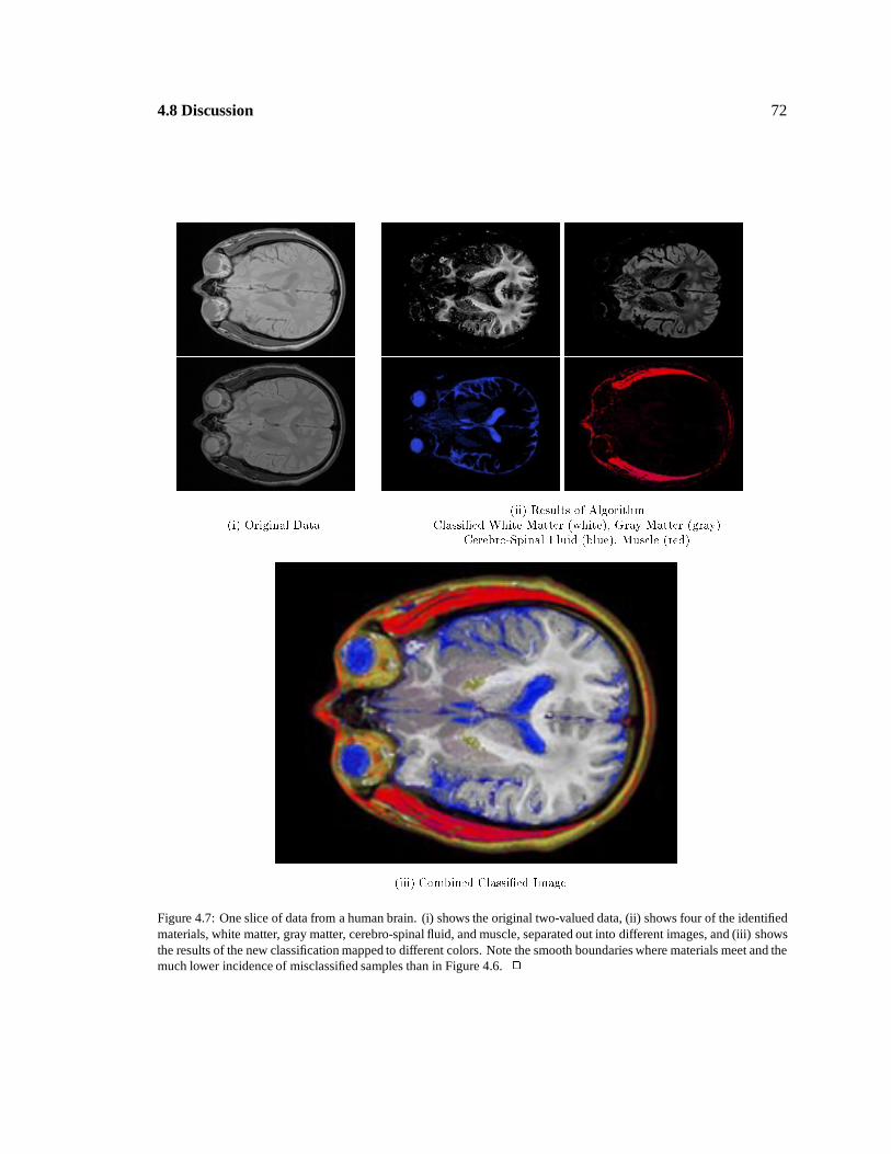
4.8 Discussion 72
(i) Original Data(ii) Results of Algorithm
Classi�ed White Matter (white), Gray Matter (gray)Cerebro-Spinal Fluid (blue), Muscle (red)
(iii) Combined Classi�ed Image
Figure 4.7: One slice of data from a human brain. (i) shows the original two-valued data, (ii) shows four of the identifiedmaterials, white matter, gray matter, cerebro-spinal fluid, and muscle, separated out into different images, and (iii) showsthe results of the new classification mapped to different colors. Note the smooth boundaries where materials meet and themuch lower incidence of misclassified samples than in Figure 4.6. 2
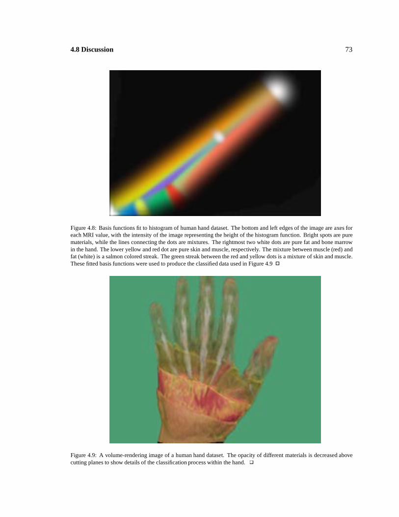
4.8 Discussion 73
Figure 4.8: Basis functions fit to histogram of human hand dataset. The bottom and left edges of the image are axes foreach MRI value, with the intensity of the image representing the height of the histogram function. Bright spots are purematerials, while the lines connecting the dots are mixtures. The rightmost two white dots are pure fat and bone marrowin the hand. The lower yellow and red dot are pure skin and muscle, respectively. The mixture between muscle (red) andfat (white) is a salmon colored streak. The green streak between the red and yellow dots is a mixture of skin and muscle.These fitted basis functions were used to produce the classified data used in Figure 4.9 2
Figure 4.9: A volume-rendering image of a human hand dataset. The opacity of different materials is decreased abovecutting planes to show details of the classification process within the hand. 2
4.8 Discussion 74
We chose two-material mixtures because surfaces between boundaries of pure materials are one of
the most important parts of computer graphics models. Voxels containing three-material mixtures
happen near lines where three materials meet, and are generally much less common, because the
dimensionality of the lines is smaller than the dimensionality of surfaces where two materials meet.
Our algorithm chooses a classification for voxels containing more than two materials from the
set of 2-material mixtures. Generally, the two largest materials in the voxel influence the choice,
producing a dataset with small artifacts where three or more materials come together.
Partial Mixtures. We note that the histograms hvox(v) for some voxel regions are not ideally
matched by a linear sum of basis functions. We address two problems here.
The first problem is that, within a small region, the assumption that we still have normally
distributed noise is no longer valid. �N models the fact that the noise no longer averages to zero, but
we do not attempt to model the change in the shape of the distribution as the region size shrinks.
The second problem is related. A small region may not contain the full range of values that
the mixture of materials can produce. As a result, the histogram over that small region is not
modeled ideally by a linear combination of pure material and mixture distributions. We investigate
an additional parameter to address this problem in Chapter 5.
We postulate that these two effects weight the optimization process such that it tends to make �N
much larger than we expect. As a result, we have found that setting the normalization factor, w(v),
to approximately 30 times the maximum value in hvox(v) gives good classification results. Smaller
values tend to allow �N to move too much, and larger values hold it constant. Without these problems
we would expect the algorithm to work best for values of w(v) equal to some small percentage of
the maximum of hvox(v). Once again, we address this problem more effectively in Chapter 5.

4.9 Conclusion 75
4.9 Conclusion
We have developed a new classification algorithm within the Bayesian framework described in
Chapter 3. The new algorithm uses histograms taken over small voxel regions to represent the
information within a voxel, and models these histograms as a linear combination of basis functions
for pure materials and for mixtures of materials. The pure material basis function is a normal
distribution, but the mixture basis function is new and is derived in Section 4.10. The new algorithm
classifies MRI data better than previous algorithms, especially near boundaries between materials,
because the histogram incorporates more information about the voxel than a single measurement
and because the histogram model explicitly incorporates boundaries between materials.
4.10 Derivation of Material PDFs
In this section we derive material PDFs that we use as basis functions (fi) for fitting histograms.
We derive two forms of basis functions: one for single, pure materials and another for two-material
mixtures (which arise due to sampling). Here is Equation 4.1, the histogram equation:
hR(v) =ZR(x)�(�(x) � v)dx (4:8)
Note that if �(x) contains additive noise n(x; s) with a particular distribution kn(v; s), then the
histogram of � with noise is the convolution in v of the normal distribution kn(v; s) with �(x)�n(x; s)
(i.e, �(x) without noise). We represent the convolution in v with the operator �v. Thus
hR(v) =R R(x)�(�(x) � v)dx
hR(v) = kn(v; s) �vR R(x)�((�(x) � n(x; s))� v)dx
(4:9)

4.10 Derivation of Material PDFs 76
4.10.1 Pure Materials
For a single pure material we assume that the measurement function has the form:
�single(x) = c + n(x; s); (4:10)
where c is the constant expected value of a measurement of the pure material, and n(x; s) is the
normally distributed noise at x with variance s.
The basis function we use to fit the histogram of the measurements of a pure material is
fsingle(v; c; s) =R R(x)�(�single(x) � v)dx
=R R(x)�(c + n(x; s)� v)dx
= kn(v; s) � R R(x)�(c � v)dx
=Qnv
i=11
sip
2�exp
��1
2
�vi�ci
si
�2�
(4:11)
Thus fsingle(v; c; s) is a normal distribution with mean c and variance s. We assume the noise is
independent in each element of vector-valued data, which for MRI appears to be reasonable.
4.10.2 Mixtures
For a mixture of two pure materials, we assume the measurement function has the form:
�double(x) = `double(x; c1; c2) + n(x; s) (4:12)
where `double approximates the band-limiting filtering process, a convolution with a box filter, by
interpolating the values within the region of mixtures linearly between c1 to c2, the mean values for
the two materials.
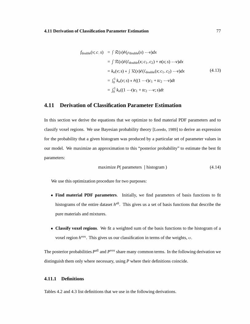
4.11 Derivation of Classification Parameter Estimation 77
fdouble(v; c; s) =R R(x)�(�double(x) � v)dx
=R R(x)�(`double(x; c1; c2) + n(x; s)� v)dx
= kn(v; s) � R R(x)�(`double(x; c1; c2) � v)dx
=R 1
0 kn(v; s) � �((1� t)c1 + tc2 � v)dt
=R 1
0 kn((1 � t)c1 + tc2 � v; s)dt
(4:13)
4.11 Derivation of Classification Parameter Estimation
In this section we derive the equations that we optimize to find material PDF parameters and to
classify voxel regions. We use Bayesian probability theory [Loredo, 1989] to derive an expression
for the probability that a given histogram was produced by a particular set of parameter values in
our model. We maximize an approximation to this “posterior probability” to estimate the best fit
parameters:
maximize P( parameters j histogram ) (4:14)
We use this optimization procedure for two purposes:
� Find material PDF parameters. Initially, we find parameters of basis functions to fit
histograms of the entire dataset hall. This gives us a set of basis functions that describe the
pure materials and mixtures.
� Classify voxel regions. We fit a weighted sum of the basis functions to the histogram of a
voxel region hvox. This gives us our classification in terms of the weights, �.
The posterior probabilities Pall and Pvox share many common terms. In the following derivation we
distinguish them only where necessary, using P where their definitions coincide.
4.11.1 Definitions
Tables 4.2 and 4.3 list definitions that we use in the following derivations.
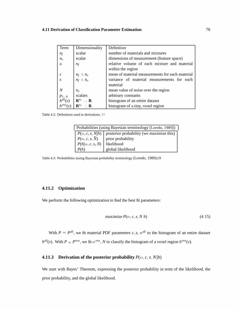
4.11 Derivation of Classification Parameter Estimation 78
Term Dimensionality Definitionnf scalar number of materials and mixturesnv scalar dimensions of measurement (feature space)� nf relative volume of each mixture and material
within the regionc nf � nv mean of material measurements for each materials nf � nv variance of material measurements for each
material�N nv mean value of noise over the regionp1:::6 scalars arbitrary constantshall(v) Rnv ! R histogram of an entire datasethvox(v) Rnv ! R histogram of a tiny, voxel region
Table 4.2: Definitions used in derivations. 2
Probabilities (using Bayesian terminology [Loredo, 1989]):P(�; c; s; �Njh) posterior probability (we maximize this)P(�; c; s; �N) prior probabilityP(hj�; c; s; �N) likelihoodP(h) global likelihood
Table 4.3: Probabilities (using Bayesian probability terminology [Loredo, 1989]) 2
4.11.2 Optimization
We perform the following optimization to find the best fit parameters:
maximize P(�; c; s; �Njh) (4:15)
With P � Pall, we fit material PDF parameters c; s, �all to the histogram of an entire dataset
hall(v). With P � Pvox, we fit �vox, �N to classify the histogram of a voxel region hvox(v).
4.11.3 Derivation of the posterior probability P(�; c; s; �Njh)
We start with Bayes’ Theorem, expressing the posterior probability in term of the likelihood, the
prior probability, and the global likelihood.

4.11 Derivation of Classification Parameter Estimation 79
P(�; c; s; �Njh) =P(�; c; s; �N)P(hj�; c; s; �N)
P(h)(4:16)
Each of the terms on the right-hand side is approximated below, using p1:::6 to denote constants
(which can be ignored during the optimization process).
Prior Probabilities. We assume that �, c, s and �N are independent, so
P(�; c; s; �N) = P(�)P(c; s)P(�N) (4:17)
Because the elements of � represent relative volumes, we require that they sum to 1 and are
positive.
P(�) =
8>>>>><>>>>>:
0 ifPnf
j=1 �j 6= 1
0 if �j < 0 or �j > 1
p1 (constant) otherwise
(4:18)
We use a different assumption for P(c; s) depending on whether we are fitting hall or hvox. For
fitting hall(v), we consider all values of c; s equally likely
Pall(c; s) = p6 (4:19)
For fitting hvox, c; s are fixed at c0; s0 (the values determined by the earlier fit to the entire data set).
Pvox(c; s) = �(c� c0; s� s0) (4:20)
For a small region, we assume that the noise vector, �N, has normal distribution with variance
�.
Pvox(�N) = p2e�Pnv
i=1(�Ni�i
)2(4:21)
For a large region, the mean noise �N should be very close to zero and hence Pall(�N) will be a delta

4.11 Derivation of Classification Parameter Estimation 80
function at �N = 0.
Pall(�N) = �(0) (4:22)
Likelihood. We approximate the likelihood P(hj�; c; s; �N) by analogy to a discrete normal dis-
tribution. We define q(v) to measure the difference between the expected histogram for particular
�; c; s; �N and a given histogram h(v)
q(v;�; c; s; �N) = h(v � �N)�nfXj=1
�jfj(v; c; s) (4:23)
Now we create a function by analogy to a normal distribution. w(v) is analogous to the variance of
q at each point of feature space.
P(hj�; c; s; �N) = p3e�12
R( q(v;�;c;s;�N )
w(v) )2dv (4:24)
Global Likelihood. Note that the denominator of Equation 4.16, P(h) is constant. It normalizes
the numerator.
Assembly of Terms.
Using the approximations discussed above, we arrive at the following expression for the posterior
probability:
P(�; c; s; �Njh) = p5P(�)P(c; s)�
e�Pnv
i=1(�Ni�i
)2��
e�R
( q(v;�;c;s;�N )w(v) )2dv
�(4:25)
For fitting hall, the mean noise is assumed to be zero. The coefficient of the exponential are
constant with respect to the parameters, so maximizing Equation 4.25 is equivalent to minimizing

4.11 Derivation of Classification Parameter Estimation 81
the argument of the exponential to find the free parameters (�all; c; s):
Eall(�all; c; s) =Z
q(v;�all; c; s)w(v)
!2
dv (4:26)
subject to P(�all) 6= 0.
For fitting hvox, the parameters c and s are fixed. Once again, the coefficients of the exponential
are constant with respect to the parameters, so maximizing Equation 4.25 is equivalent to minimizing
the argument of the exponential to find the free parameters (�vox; �N):
Evox(�vox; �N) =nvXi=1
� �Ni
�i
�2
+Z �
q(v;�vox; �N)w(v)
�2
dv (4:27)
subject to P(�vox) 6= 0.
As described in Equation 4.6, Section 4.6, Equation 4.27 is minimized to estimate volume ratio
densities �vox and the mean noise vector �N.
82
Chapter 5
Bayesian Classification Algorithms B and
C: Boundary Distance
In this chapter we describe two new classification techniques developed within the Bayesian frame-
work of Chapter 3.
The techniques we develop here are similar to that of Chapter 4; as before, the voxel-info
consists of histograms taken over voxel regions. The significant differences between the techniques
are that we use new histogram basis functions and that the dataset parameters are estimated using a
different algorithm.
The new histogram basis functions model voxels near boundaries between two materials. The
histogram model has a single parameter: the distance from the center of the voxel to the boundary.
The basis functions fit histograms of real datasets better than the partial volume mixtures algorithm,
but at the cost of somewhat greater computational expense. The resulting distance parameter is
particularly useful in making models of objects because it measures the distance from surface
boundaries between materials. These boundaries are generally boundaries between parts of objects
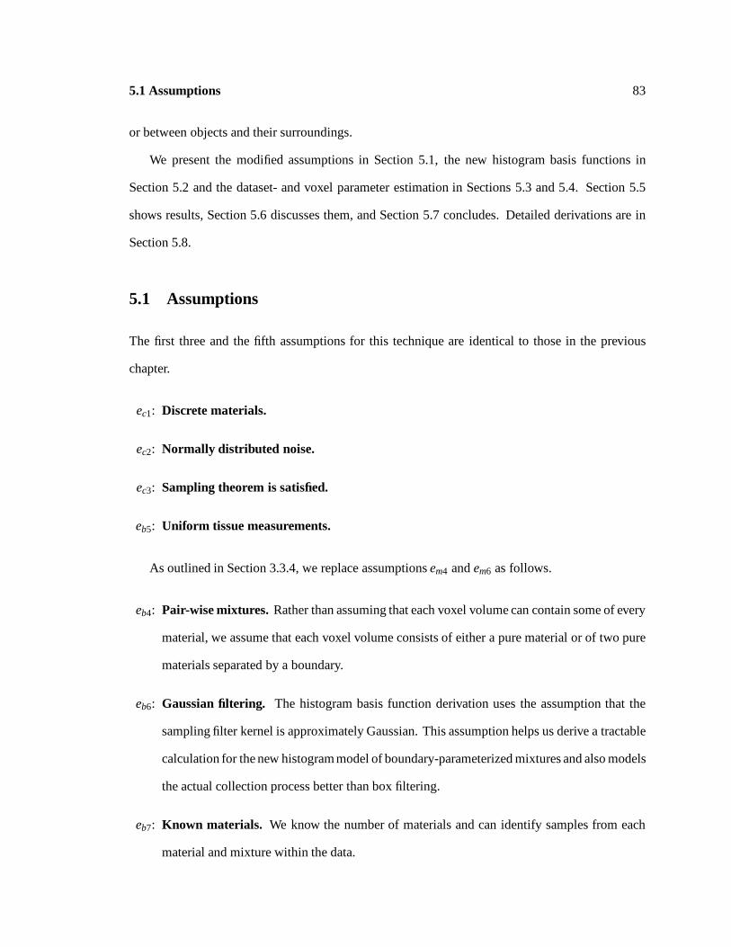
5.1 Assumptions 83
or between objects and their surroundings.
We present the modified assumptions in Section 5.1, the new histogram basis functions in
Section 5.2 and the dataset- and voxel parameter estimation in Sections 5.3 and 5.4. Section 5.5
shows results, Section 5.6 discusses them, and Section 5.7 concludes. Detailed derivations are in
Section 5.8.
5.1 Assumptions
The first three and the fifth assumptions for this technique are identical to those in the previous
chapter.
ec1: Discrete materials.
ec2: Normally distributed noise.
ec3: Sampling theorem is satisfied.
eb5: Uniform tissue measurements.
As outlined in Section 3.3.4, we replace assumptions em4 and em6 as follows.
eb4: Pair-wise mixtures. Rather than assuming that each voxel volume can contain some of every
material, we assume that each voxel volume consists of either a pure material or of two pure
materials separated by a boundary.
eb6: Gaussian filtering. The histogram basis function derivation uses the assumption that the
sampling filter kernel is approximately Gaussian. This assumption helps us derive a tractable
calculation for the new histogram model of boundary-parameterized mixtures and also models
the actual collection process better than box filtering.
eb7: Known materials. We know the number of materials and can identify samples from each
material and mixture within the data.

5.2 Histogram Basis Functions 84
5.2 Histogram Basis Functions
Once again we use two types of histogram basis functions, one for pure materials and one for
mixtures of materials. The basis function for pure materials remains a normal distribution. The
basis function for a mixture now has an additional parameter that defines the distance from the
center of a voxel to a boundary between materials (see Figure 5.1).
From the assumptions and Equation. 4.1 we derive the equation for a pure-material basis
function. Because the data collection process band-limits the noise, and because we are looking
at histograms over very small regions, the noise is not normally distributed. We divide the noise
into two components, one that is constant over a voxel (with mean c and standard deviation � over
the dataset), and one that is normally distributed around the constant component (with mean 0 and
standard deviation s over a voxel). The equation for a single material, then, is a normal distribution
with center c + �N and variance �2:
fsingle(v; �N; c; s) =nvYi=1
1
sip
2�exp
�1
2
nvXi=1
�v � (c + �N)
si
�2!
(5:1)
Dataset parameters for this basis function are c, s, and �. Because �N is constant within a voxel,
but varies over the dataset with a normal distribution, � also becomes a dataset parameter.
From the assumptions and Equation. 4.1 we derive the equation for a mixture basis function.
The function uses the same parameters for its pure materials components and adds two additional
parameters d and kw, as shown in Figure 5.1. See Figures 5.2 and 5.3 for examples.
fboundary(v; d; �N; c; s; kw) =
kn(v; s) ���
H(d + kh2 � ke(v)
kw) � H(d � kh
2 � ke(v)kw
)� ��� eke(v)p�
(c2�c1)kw
���� (5:2)
where ke(v) = erf�1( c1+c2�2vc1�c2
) and H(x) is the Heaviside, or step, function. The derivation follows
from Equation. 4.1 evaluated over a region centered at distance d from a boundary between two
materials. The boundary is assumed to be planar and the function low-pass filtered uniformly in all
directions so that the sampling theorem is satisfied. kw depends on the width of the sampling kernel
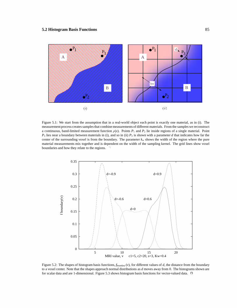
5.2 Histogram Basis Functions 85
A
B
P1
P2
P3
(i)
A
B
P1
P2
P3
kw
d
(ii)
Figure 5.1: We start from the assumption that in a real-world object each point is exactly one material, as in (i). Themeasurementprocess creates samples that combine measurements of different materials. From the samples we reconstructa continuous, band-limited measurement function �(x). Points P1 and P2 lie inside regions of a single material. PointP3 lies near a boundary between materials in (i), and so in (ii) P3 is shown with a parameter d that indicates how far thecenter of the surrounding voxel is from the boundary. The parameter kw shows the width of the region where the purematerial measurements mix together and is dependent on the width of the sampling kernel. The grid lines show voxelboundaries and how they relate to the regions. 2
0
0.05
0.1
0.15
0.2
0.25
0.3
0.35
5 10 15 20
f bo
unda
ry(v
)
MRI value, v c1=5, c2=20, s=3, Kw=0.4
d=0
d=0.6d=-0.6
d=0.9d=-0.9
Figure 5.2: The shapes of histogram basis functions, fboundary (v), for different values of d, the distance from the boundaryto a voxel center. Note that the shapes approach normal distributions as d moves away from 0. The histograms shown arefor scalar data and are 1-dimensional. Figure 5.3 shows histogram basis functions for vector-valued data. 2
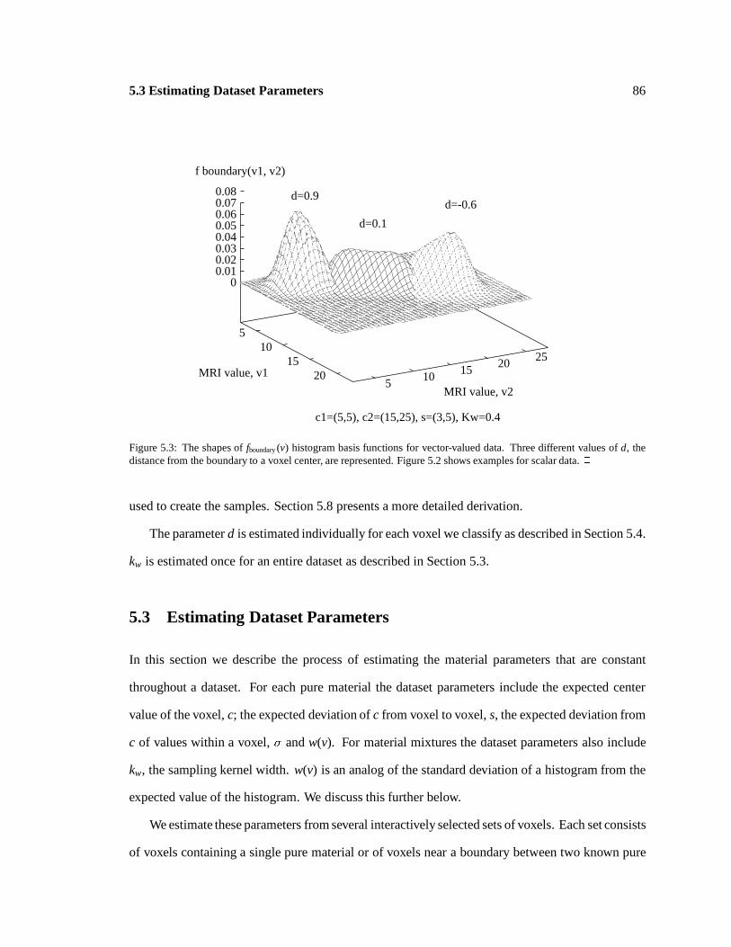
5.3 Estimating Dataset Parameters 86
d=0.9d=-0.6
d=0.1
c1=(5,5), c2=(15,25), s=(3,5), Kw=0.4
510
1520
5 10 15 20 25
00.010.020.030.040.050.060.070.08
MRI value, v1
MRI value, v2
f boundary(v1, v2)
Figure 5.3: The shapes of fboundary (v) histogram basis functions for vector-valued data. Three different values of d, thedistance from the boundary to a voxel center, are represented. Figure 5.2 shows examples for scalar data. 2
used to create the samples. Section 5.8 presents a more detailed derivation.
The parameter d is estimated individually for each voxel we classify as described in Section 5.4.
kw is estimated once for an entire dataset as described in Section 5.3.
5.3 Estimating Dataset Parameters
In this section we describe the process of estimating the material parameters that are constant
throughout a dataset. For each pure material the dataset parameters include the expected center
value of the voxel, c; the expected deviation of c from voxel to voxel, s, the expected deviation from
c of values within a voxel, � and w(v). For material mixtures the dataset parameters also include
kw, the sampling kernel width. w(v) is an analog of the standard deviation of a histogram from the
expected value of the histogram. We discuss this further below.
We estimate these parameters from several interactively selected sets of voxels. Each set consists
of voxels containing a single pure material or of voxels near a boundary between two known pure
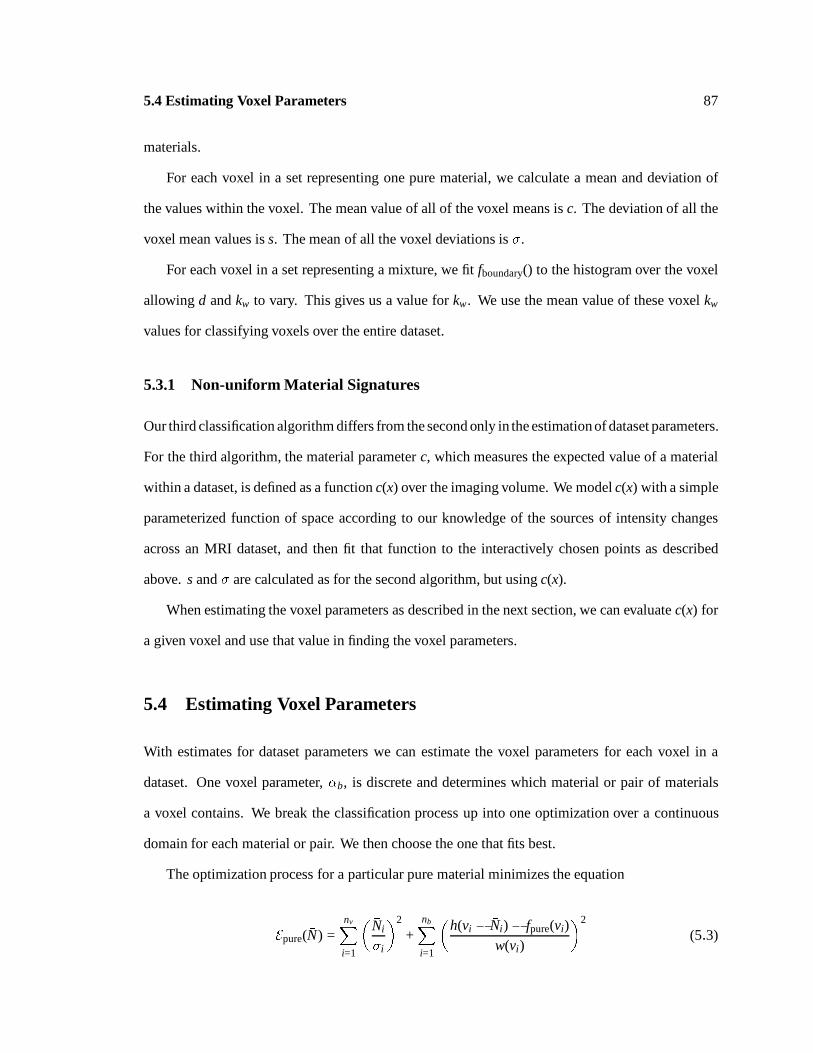
5.4 Estimating Voxel Parameters 87
materials.
For each voxel in a set representing one pure material, we calculate a mean and deviation of
the values within the voxel. The mean value of all of the voxel means is c. The deviation of all the
voxel mean values is s. The mean of all the voxel deviations is �.
For each voxel in a set representing a mixture, we fit fboundary() to the histogram over the voxel
allowing d and kw to vary. This gives us a value for kw. We use the mean value of these voxel kw
values for classifying voxels over the entire dataset.
5.3.1 Non-uniform Material Signatures
Our third classification algorithm differs from the second only in the estimation of dataset parameters.
For the third algorithm, the material parameter c, which measures the expected value of a material
within a dataset, is defined as a function c(x) over the imaging volume. We model c(x) with a simple
parameterized function of space according to our knowledge of the sources of intensity changes
across an MRI dataset, and then fit that function to the interactively chosen points as described
above. s and � are calculated as for the second algorithm, but using c(x).
When estimating the voxel parameters as described in the next section, we can evaluate c(x) for
a given voxel and use that value in finding the voxel parameters.
5.4 Estimating Voxel Parameters
With estimates for dataset parameters we can estimate the voxel parameters for each voxel in a
dataset. One voxel parameter, �b, is discrete and determines which material or pair of materials
a voxel contains. We break the classification process up into one optimization over a continuous
domain for each material or pair. We then choose the one that fits best.
The optimization process for a particular pure material minimizes the equation
Epure(�N) =nvXi=1
� �Ni
�i
�2
+nbXi=1
�h(vi � �Ni)� fpure(vi)
w(vi)
�2
(5:3)
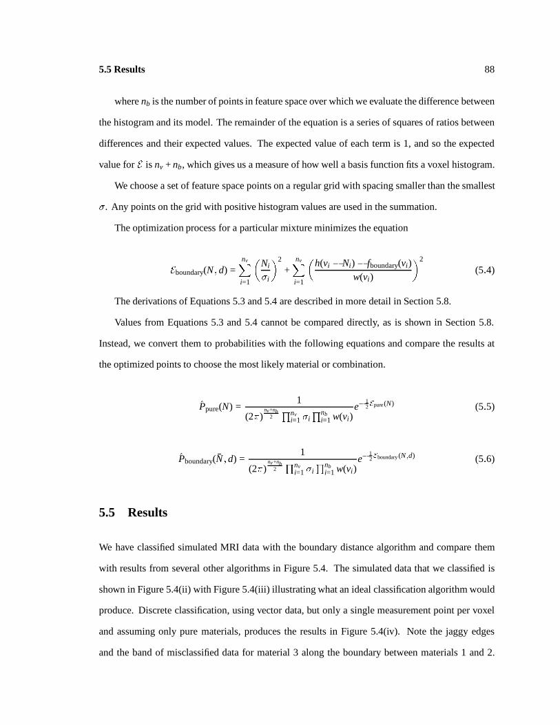
5.5 Results 88
where nb is the number of points in feature space over which we evaluate the difference between
the histogram and its model. The remainder of the equation is a series of squares of ratios between
differences and their expected values. The expected value of each term is 1, and so the expected
value for E is nv + nb, which gives us a measure of how well a basis function fits a voxel histogram.
We choose a set of feature space points on a regular grid with spacing smaller than the smallest
�. Any points on the grid with positive histogram values are used in the summation.
The optimization process for a particular mixture minimizes the equation
Eboundary(�N; d) =nvXi=1
� �Ni
�i
�2
+nvXi=1
�h(vi � �Ni)� fboundary(vi)
w(vi)
�2
(5:4)
The derivations of Equations 5.3 and 5.4 are described in more detail in Section 5.8.
Values from Equations 5.3 and 5.4 cannot be compared directly, as is shown in Section 5.8.
Instead, we convert them to probabilities with the following equations and compare the results at
the optimized points to choose the most likely material or combination.
Ppure(�N) =1
(2�)nv+nb
2Qnv
i=1 �iQnb
i=1 w(vi)e�
12Epure(�N) (5:5)
Pboundary(�N; d) =1
(2�)nv+nb
2Qnv
i=1 �iQnb
i=1 w(vi)e�
12Eboundary (�N;d) (5:6)
5.5 Results
We have classified simulated MRI data with the boundary distance algorithm and compare them
with results from several other algorithms in Figure 5.4. The simulated data that we classified is
shown in Figure 5.4(ii) with Figure 5.4(iii) illustrating what an ideal classification algorithm would
produce. Discrete classification, using vector data, but only a single measurement point per voxel
and assuming only pure materials, produces the results in Figure 5.4(iv). Note the jaggy edges
and the band of misclassified data for material 3 along the boundary between materials 1 and 2.
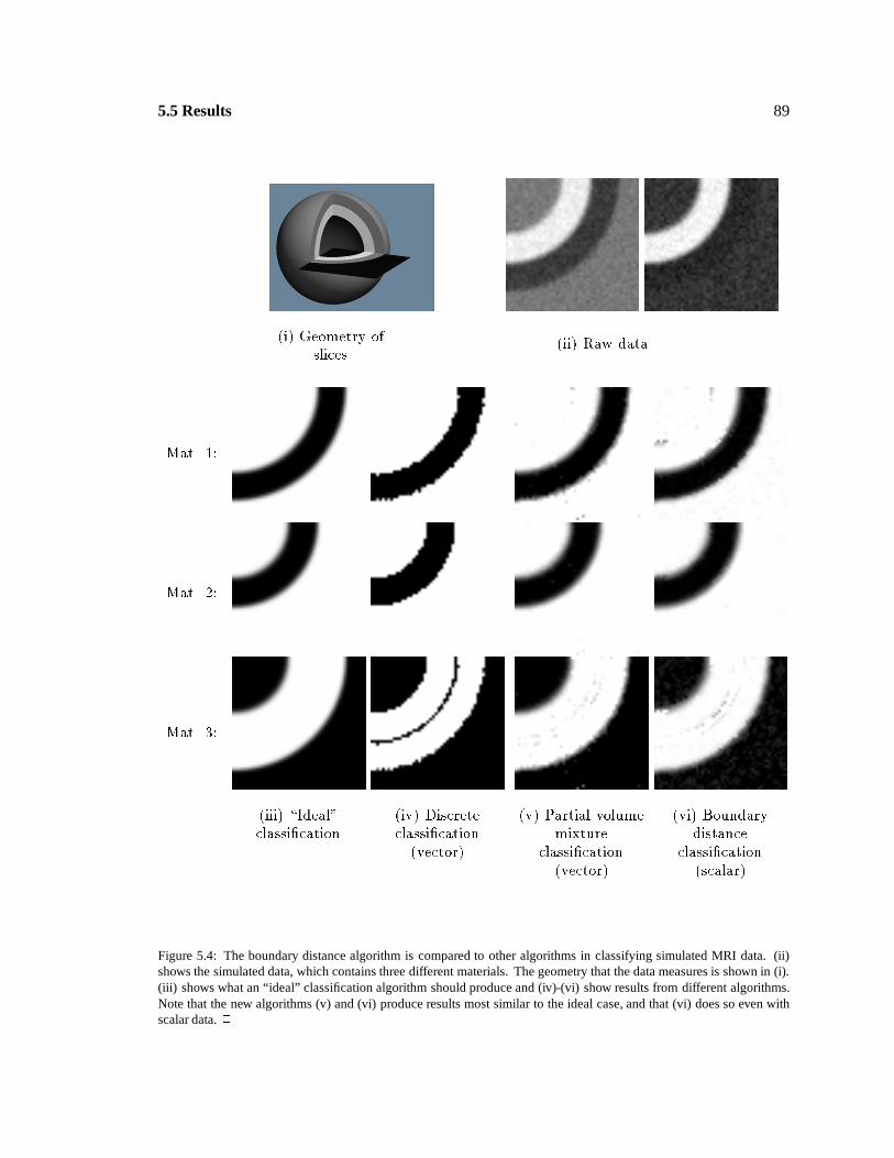
5.5 Results 89
(i) Geometry ofslices
(ii) Raw data
Mat. 1:
Mat. 2:
Mat. 3:
(iii) \Ideal"classi�cation
(iv) Discreteclassi�cation(vector)
(v) Partial volumemixture
classi�cation(vector)
(vi) Boundarydistance
classi�cation(scalar)
Figure 5.4: The boundary distance algorithm is compared to other algorithms in classifying simulated MRI data. (ii)shows the simulated data, which contains three different materials. The geometry that the data measures is shown in (i).(iii) shows what an “ideal” classification algorithm should produce and (iv)-(vi) show results from different algorithms.Note that the new algorithms (v) and (vi) produce results most similar to the ideal case, and that (vi) does so even withscalar data. 2
5.6 Discussion 90
Figure 5.4(v) and Figure 5.4(vi) show the partial volume mixtures algorithm from Chapter 4 and
the boundary distance algorithm from this chapter. Note that even with scalar data, the boundary
distance algorithm achieves results very close to the ideal case.
5.6 Discussion
Ambiguous classification. For a voxel that is well within a region of pure material A, the algorithm
sometimes correctly classifies the voxel as pure material A, and sometimes classifies it as a mixture of
A and a very small amount of some other material. Both solutions are physically reasonable because
the mixture basis functions approach a normal distribution as the boundary distance parameter d
moves away from zero.
Similarly, two different mixtures, each containing material A, can match a voxel that is within
a region of pure material A. Again, the choice is not critical.
Sensitivity to interactively selected material classes. The results of the algorithm are highly
dependent on the material points selected interactively to represent each pure material and each
pair of materials. These points must be selected carefully, and should come from a set of points
that actually represent a single consistent material. Representing points from two materials as one
material can create a situation where the distributions of the sample values do not match a normal
distribution, and the classification results are less accurate.
The algorithm could verify that the selected points are normally distributed to identify the
problem and report it to the user.
Sensitivity to contrast between materials. The classification is sensitive to the contrast-to-noise
ratio between different materials. If this ratio is too small, materials cannot be distinguished. This
requirement is fed back to the data-collection process described in Chapter 2.

5.7 Conclusion 91
Computational expense. The implementations described in this chapter are computationally
expensive. The optimization process must be run on each voxel in a dataset. At ten voxels
per second, a medium-sized dataset of 256 � 256 � 64 voxels runs in about 5 days. Through
approximations it may be possible to reduce this time significantly.
The algorithm processes each voxel independently, and so is highly amenable to a domain-
decomposition parallel solution. In fact, we have run it on a network of ten HP 9000/700 and DEC
Alpha workstations and gotten a speedup of almost ten in classifying medium to large datasets.
More sophisticated geometric basis functions. The basis functions that we have developed
model the two most common geometric cases: samples within regions of pure material and samples
near surface boundaries. Additional basis functions, however, could model other geometries and
create more accurate models. Examples include samples near edges where three materials come
together, or points near membranes that are thinner than the sample spacing, where, again, three
materials would have an effect on the measurement.
Incorporating additional global information. Except for the interpolation of samples, we cur-
rently classify each voxel without regard to its neighbors and without directly using the interactively
selected representative points for each material. Both types of information could be incorporated
into the prior probability estimates to influence the classification process.
5.7 Conclusion
We have presented two new classification algorithms, one a variation on the other, built within the
Bayesian framework we described in Chapter 3. The algorithms are based on a more accurate
model of the MRI process than the algorithm of Chapter 4, and so produce better results, but are
computationally more expensive.
5.8 Detailed Derivations 92
5.8 Detailed Derivations
This section derives the boundary distance histogram basis functions for pure materials and for
mixtures as well as the prior probability optimization equations used in Section 5.4.
5.8.1 Pure Histogram Basis Function
The derivation for pure material basis functions is identical to that of Ch. 4 and is in Section 4.10.1.
5.8.2 Mixture Histogram Basis Function
For a sample taken near a boundary between two pure materials we start with an object that spans
all of 3-space and that has two materials separated by a planar boundary. Because we are going to
use a rotationally symmetric Gaussian sampling kernel, we can perform a change of coordinates on
our object to make the planar boundary pass through the origin and be perpendicular to the x0-axis.
The object function is:
v(x) =
8><>:
c1 if x0 < 0
c2 if x0 > 0(5:7)
Our measurement function is:
�boundary(x) =Z Z Z
k(x0)k(x1)k(x2)v(x � x)dx2dx1dx0 + n(x; s) (5:8)
where k(x) is the 1-D Gaussian sampling kernel. Its width is determined by an implicit parameter
kw. v(x � x) is independent of x1 and x2, so
�boundary(x) =Z
k(x0)v(x � x)�Z Z
k(x1)k(x2)dx2dx1
�dx0 + n(x; s) (5:9)

5.8 Detailed Derivations 93
The term in parentheses is one, and so:
�boundary(x) =Z 1
�1k(x0)v(x0 � x0)dx0 + n(x; s) (5:10)
We assume a Gaussian kernel function:
k(x) =1
kwp�
e��
xkw
�2
(5:11)
By evaluating the integrals we find:
�boundary(x) =R1�1 k(x0)v(x0 � x0)dx0 + n(x; s)
= c1R x0�1 k(x0)dx0 + c2
R1x0
k(x0)dx0 + n(x; s)
= 12 (c2 + c1 + (c2 � c1)erf(kwx0))) + n(x; s)
(5:12)
This measurement function can now be substituted into Equation. 4.1 to derive the boundary
basis function:
fboundary(v; d; �N; c; s; kw) =R R(x)�(fboundary(x) � v)dx
=R R(x)�(1
2 (c2 + c1 + (c2 � c1)erf(kwx0))) + n(x; s)� v)dx
= kn(v; s) �vR R(x)�(1
2 (c2 + c1 + (c2 � c1)erf(kwx0)))� v)dx
(5:13)
We define the region R(x) as a rectangular solid kh on a side and distance d from the boundary
at 0. Because the integrand depends only on x0, we can reduce this to a single integral
= kn(v; s) � k2h
Z d+kh2
d� kh2
�(12
(c2 + c1 + (c2 � c1)erf(kwx0))) � v)dx0 (5:14)
= kn(v; s) � �
H(d +kh
2� ke(v)
kw) � H(d � kh
2� ke(v)
kw)� ����� eke(v)p�
(c2 � c1)kw
�����!
(5:15)
where ke(v) = erf�1( c1+c2�2vc1�c2
) and H(x) is the Heaviside, or step, function.

5.8 Detailed Derivations 94
H(x) =
8><>:
0 if x < 0
1 if x > 0(5:16)
We refer to the right operand of the convolution as r(v)
r(v) =
�H(d +
kh
2� ke(v)
kw)� H(d � kh
2� ke(v)
kw)� ����� eke(v)p�
(c2 � c1)kw
�����!
(5:17)
fboundary(v) = kn(v) � r(v) (5:18)
Implementation Considerations
Our implementation evaluates this function by creating a piecewise-linear approximation to r(v)
and summing the convolutions of the linear pieces. r(v) is non-zero only between
12
(c2 + c1 + (c2 � c1)erf(kw(d +kh
2))) (5:19)
and
12
(c2 + c1 + (c2 � c1)erf(kw(d � kh
2))) (5:20)
We evaluate r(v) at regularly spaced points between those endpoints, scale the resulting values to
preserve the total integral, evaluate the convolution, and sum the results.
5.8.3 Pure Material Parameter Estimation
We wish to be able to evaluate
P(�Njh) =P(�N)P(hj�N)
P(h)(5:21)
where h is the histogram over a voxel and �N is the voxel parameter for a pure material.

5.8 Detailed Derivations 95
Prior probability is defined as
P(�N) =1
(2�)nv2Qnv
i=1 �i
e�12
Pnvi=1
��Ni�i
�2
(5:22)
Likelihood is defined by analogy to a multi-dimensional normal distribution. We choose nb points
in feature space and calculate the difference between the histogram model and the histogram at those
points.
P(hj�N) =1
(2�)nb2Qnb
i=1 w(vi)e� 1
2
Pnbi=1
�h(vi��Ni)�fpure (vi)
w(vi)
�2
(5:23)
Global likelihood is a constant as in Section 4.11.3.
Assembly of prior probability.
P(�Njh) =1
P(h)1
(2�)nv+nb
2Qnv
i=1 �iQnb
i=1 w(vi)e� 1
2
�Pnvi=1
��Ni�i
�2+Pnb
i=1
�h(vi��Ni)�fpure (vi)
w(vi)
�2�
(5:24)
Because the coefficient of the exponential is constant with respect to the arguments of P(�Njh),
maximizing P(�Njh) is equivalent to minimizing:
Epure(�N) =nvXi=1
� �Ni
�i
�2
+nbXi=1
�h(vi � �Ni)� fpure(vi)
w(vi)
�2
(5:25)
In comparing the optimization result among different materials, we convert to probabilities,
neglecting the global likelihood, which is not a function of the material.
Ppure(�N) =1
(2�)nv+nb
2Qnv
i=1 �iQnb
i=1 w(vi)e�
12Epure(�N) (5:26)
5.8.4 Material Mixture Parameter Estimation
We wish to be able to evaluate
5.8 Detailed Derivations 96
P(�N; djh) =P(�N; d)P(hj�N; d)
P(h)(5:27)
where �N and d are voxel parameters and h is the histogram over a voxel.
The derivation follows that of the previous section.
Prior probability is defined as
P(�N; d) = P(�N)P(d) (5:28)
P(�N) is identical to Equation 5.22.
Effects from a boundary do not occur at significant distances from the boundary. We define
significant distance as 3 times the width of the spatial sampling kernel and create a probability
density function for P(d) that integrates to one:
P(d) =
8><>:
16 if � 3 < d < 3
0 otherwise(5:29)
Likelihood is defined in the same manner as Equation 5.23.
P(hj�N; d) =1
(2�)nb2Qnb
i=1 w(vi)e� 1
2
Pnbi=1
�h(vi��Ni)�fboundary (vi)
w(vi)
�2
(5:30)
Global likelihood is a constant as in Chapter 4.
Assembly of prior probability.
P(�N; djh) =1
P(h)1
(2�)nv+nb
2Qnv
i=1 �iQnb
i=1 w(vi)e� 1
2
Pnvi=1
��Ni�i
�2+Pnb
i=1
�h(vi��Ni)�fboundary (vi)
w(vi)
�2
(5:31)
Because the coefficient of the exponential is constant with respect to the arguments of P(�N; djh),
maximizing P(�N; djh) is equivalent to minimizing:
5.8 Detailed Derivations 97
Eboundary(�N; d) =nvXi=1
� �Ni
�i
�2
+nbXi=1
�h(vi � �Ni)� fboundary(vi)
w(vi)
�2
(5:32)
In comparing the optimization result among different materials, we convert to probabilities,
neglecting the global likelihood, which is not a function of the material mixture.
Pboundary(�N; d) =1
(2�)nv+nb
2Qnv
i=1 �iQnb
i=1 w(vi)e�
12Eboundary (v;d) (5:33)
98
PART III
Applications
The following two chapters describe computer graphics applications that use the
data collection and classification techniques of the earlier chapters. Chapter 6
describes a taxonomy of computer graphics models and Chapter 7 describes a
new algorithm for directly volume-rendering deformed volume data.

99
Chapter 6
Model Building
A major unsolved problem in computer graphics is that of making high-quality models. Tradi-
tionally, models have consisted of interactively or algorithmically described collections of graphics
primitives such as polygons or patches. The process of constructing these models is painstaking
and often misses features and behavior that we wish to model.
In this chapter we present a taxonomy of computer graphics models that can be created from
classified sampled MRI data. We use results from the earlier chapters to create examples of both
static and dynamic models of objects from MRI measurements. These new results illustrate the
utility of the data-collection and classification processes.
Many of the goals used in developing the data-collection and tissue-classification algorithms
derive from requirements of the model-extraction process, providing feedback to those earlier stages
of the pipeline.
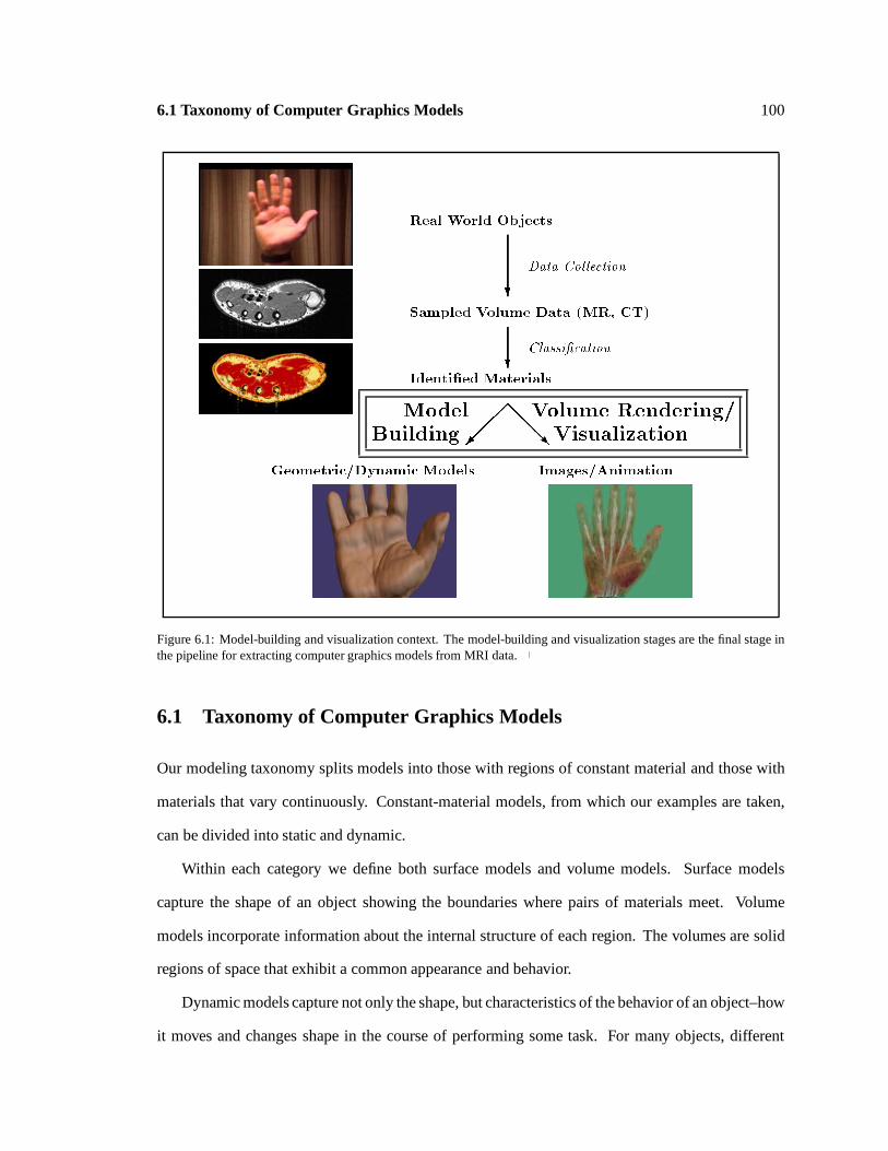
6.1 Taxonomy of Computer Graphics Models 100
Real World Objects
Sampled Volume Data (MR, CT)
Identi�ed Materials
Geometric/Dynamic Models Images/Animation
Data Collection
Classi�cation
Model Volume Rendering/Building Visualization
??
??
@@@R
@@@R
���
���
Figure 6.1: Model-building and visualization context. The model-building and visualization stages are the final stage inthe pipeline for extracting computer graphics models from MRI data. 2
6.1 Taxonomy of Computer Graphics Models
Our modeling taxonomy splits models into those with regions of constant material and those with
materials that vary continuously. Constant-material models, from which our examples are taken,
can be divided into static and dynamic.
Within each category we define both surface models and volume models. Surface models
capture the shape of an object showing the boundaries where pairs of materials meet. Volume
models incorporate information about the internal structure of each region. The volumes are solid
regions of space that exhibit a common appearance and behavior.
Dynamic models capture not only the shape, but characteristics of the behavior of an object–how
it moves and changes shape in the course of performing some task. For many objects, different
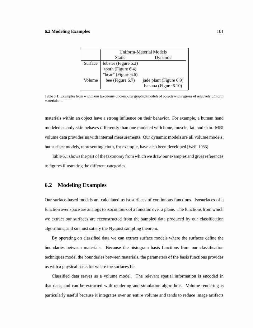
6.2 Modeling Examples 101
Uniform-Material ModelsStatic Dynamic
Surface lobster (Figure 6.2)tooth (Figure 6.4)
“bear” (Figure 6.6)Volume bee (Figure 6.7) jade plant (Figure 6.9)
banana (Figure 6.10)
Table 6.1: Examples from within our taxonomy of computer graphics models of objects with regions of relatively uniformmaterials. 2
materials within an object have a strong influence on their behavior. For example, a human hand
modeled as only skin behaves differently than one modeled with bone, muscle, fat, and skin. MRI
volume data provides us with internal measurements. Our dynamic models are all volume models,
but surface models, representing cloth, for example, have also been developed [Weil, 1986].
Table 6.1 shows the part of the taxonomy from which we draw our examples and gives references
to figures illustrating the different categories.
6.2 Modeling Examples
Our surface-based models are calculated as isosurfaces of continuous functions. Isosurfaces of a
function over space are analogs to isocontours of a function over a plane. The functions from which
we extract our surfaces are reconstructed from the sampled data produced by our classification
algorithms, and so must satisfy the Nyquist sampling theorem.
By operating on classified data we can extract surface models where the surfaces define the
boundaries between materials. Because the histogram basis functions from our classification
techniques model the boundaries between materials, the parameters of the basis functions provides
us with a physical basis for where the surfaces lie.
Classified data serves as a volume model. The relevant spatial information is encoded in
that data, and can be extracted with rendering and simulation algorithms. Volume rendering is
particularly useful because it integrates over an entire volume and tends to reduce image artifacts
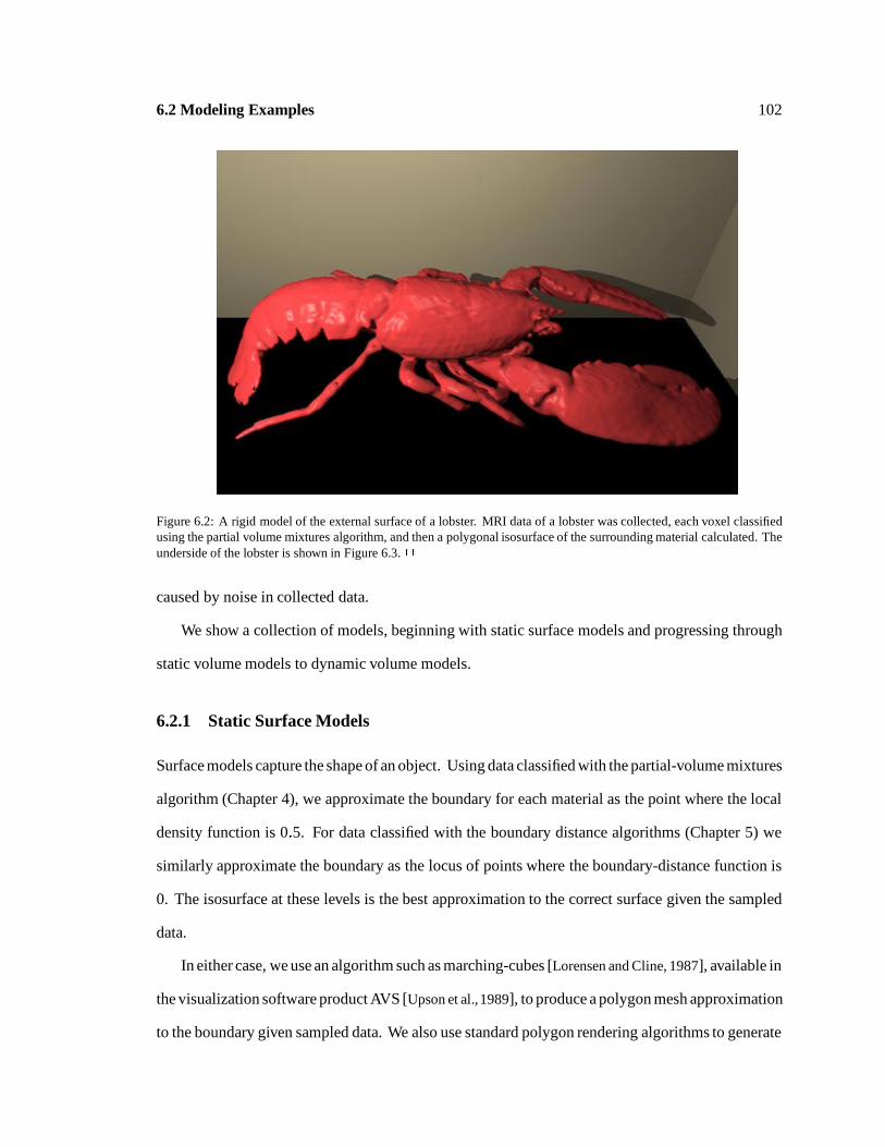
6.2 Modeling Examples 102
Figure 6.2: A rigid model of the external surface of a lobster. MRI data of a lobster was collected, each voxel classifiedusing the partial volume mixtures algorithm, and then a polygonal isosurface of the surrounding material calculated. Theunderside of the lobster is shown in Figure 6.3. 2
caused by noise in collected data.
We show a collection of models, beginning with static surface models and progressing through
static volume models to dynamic volume models.
6.2.1 Static Surface Models
Surface models capture the shape of an object. Using data classified with the partial-volume mixtures
algorithm (Chapter 4), we approximate the boundary for each material as the point where the local
density function is 0:5. For data classified with the boundary distance algorithms (Chapter 5) we
similarly approximate the boundary as the locus of points where the boundary-distance function is
0. The isosurface at these levels is the best approximation to the correct surface given the sampled
data.
In either case, we use an algorithm such as marching-cubes [Lorensen and Cline, 1987], available in
the visualization software product AVS [Upson et al.,1989], to produce a polygon mesh approximation
to the boundary given sampled data. We also use standard polygon rendering algorithms to generate
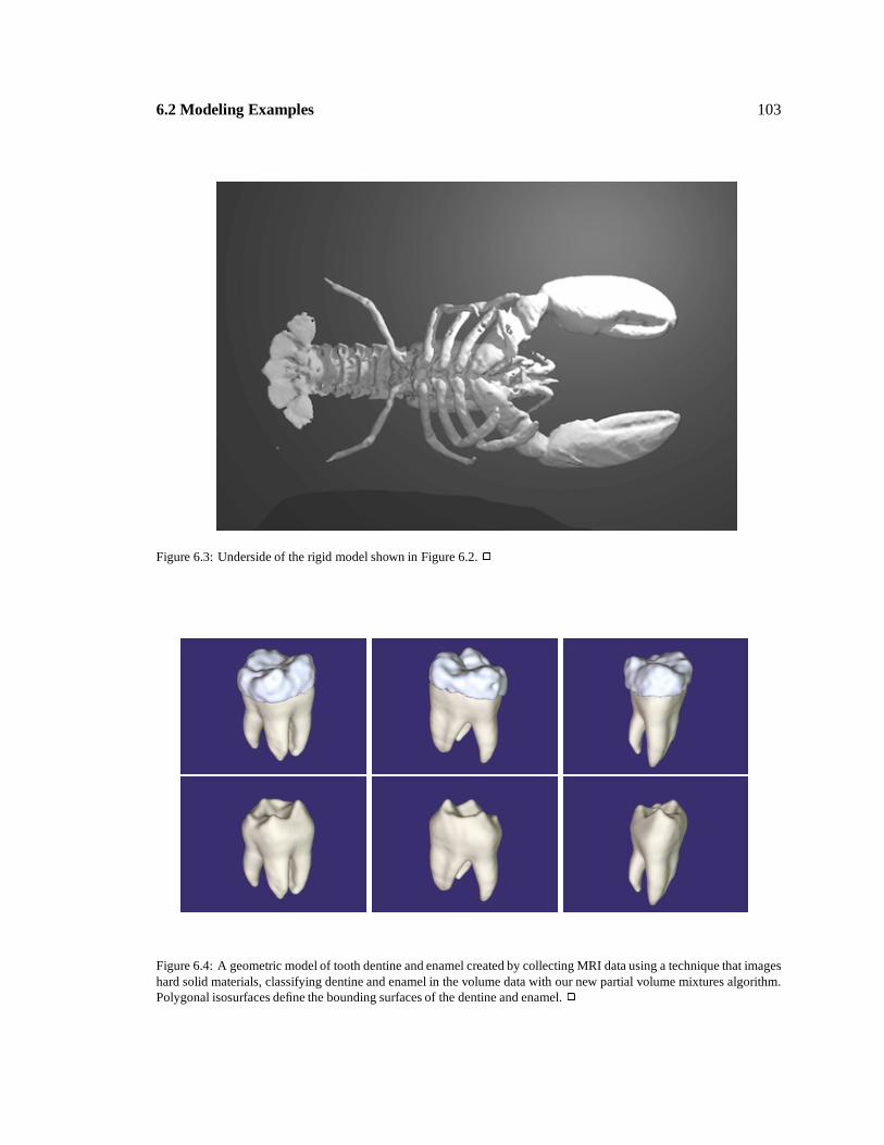
6.2 Modeling Examples 103
Figure 6.3: Underside of the rigid model shown in Figure 6.2. 2
Figure 6.4: A geometric model of tooth dentine and enamel created by collecting MRI data using a technique that imageshard solid materials, classifying dentine and enamel in the volume data with our new partial volume mixtures algorithm.Polygonal isosurfaces define the bounding surfaces of the dentine and enamel. 2
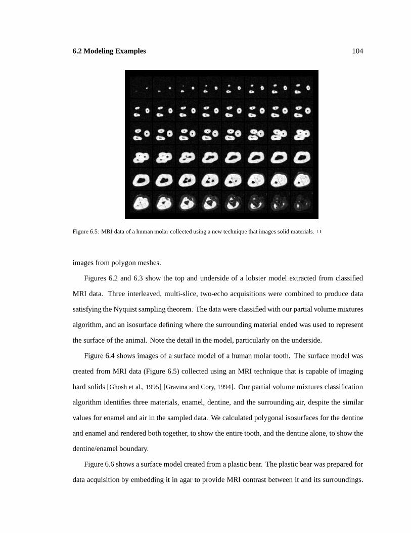
6.2 Modeling Examples 104
Figure 6.5: MRI data of a human molar collected using a new technique that images solid materials. 2
images from polygon meshes.
Figures 6.2 and 6.3 show the top and underside of a lobster model extracted from classified
MRI data. Three interleaved, multi-slice, two-echo acquisitions were combined to produce data
satisfying the Nyquist sampling theorem. The data were classified with our partial volume mixtures
algorithm, and an isosurface defining where the surrounding material ended was used to represent
the surface of the animal. Note the detail in the model, particularly on the underside.
Figure 6.4 shows images of a surface model of a human molar tooth. The surface model was
created from MRI data (Figure 6.5) collected using an MRI technique that is capable of imaging
hard solids [Ghosh et al., 1995] [Gravina and Cory, 1994]. Our partial volume mixtures classification
algorithm identifies three materials, enamel, dentine, and the surrounding air, despite the similar
values for enamel and air in the sampled data. We calculated polygonal isosurfaces for the dentine
and enamel and rendered both together, to show the entire tooth, and the dentine alone, to show the
dentine/enamel boundary.
Figure 6.6 shows a surface model created from a plastic bear. The plastic bear was prepared for
data acquisition by embedding it in agar to provide MRI contrast between it and its surroundings.
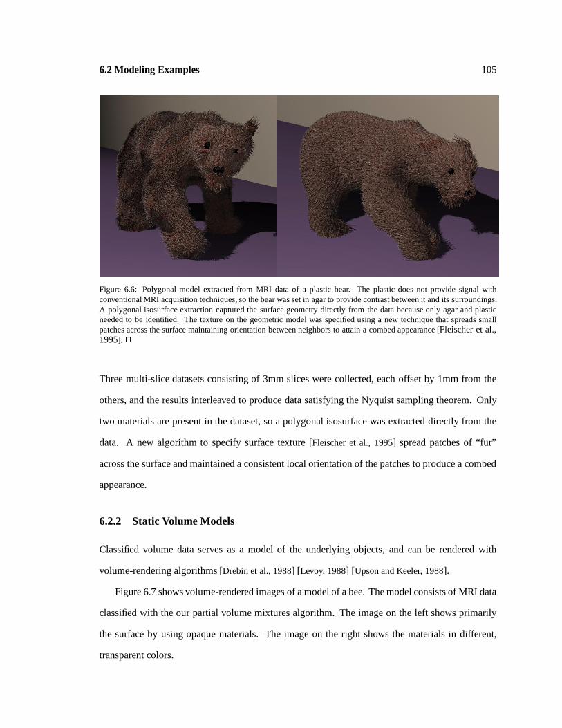
6.2 Modeling Examples 105
Figure 6.6: Polygonal model extracted from MRI data of a plastic bear. The plastic does not provide signal withconventional MRI acquisition techniques, so the bear was set in agar to provide contrast between it and its surroundings.A polygonal isosurface extraction captured the surface geometry directly from the data because only agar and plasticneeded to be identified. The texture on the geometric model was specified using a new technique that spreads smallpatches across the surface maintaining orientation between neighbors to attain a combed appearance [Fleischer et al.,1995]. 2
Three multi-slice datasets consisting of 3mm slices were collected, each offset by 1mm from the
others, and the results interleaved to produce data satisfying the Nyquist sampling theorem. Only
two materials are present in the dataset, so a polygonal isosurface was extracted directly from the
data. A new algorithm to specify surface texture [Fleischer et al., 1995] spread patches of “fur”
across the surface and maintained a consistent local orientation of the patches to produce a combed
appearance.
6.2.2 Static Volume Models
Classified volume data serves as a model of the underlying objects, and can be rendered with
volume-rendering algorithms [Drebin et al., 1988] [Levoy, 1988] [Upson and Keeler, 1988].
Figure 6.7 shows volume-rendered images of a model of a bee. The model consists of MRI data
classified with the our partial volume mixtures algorithm. The image on the left shows primarily
the surface by using opaque materials. The image on the right shows the materials in different,
transparent colors.

6.2 Modeling Examples 106
Figure 6.7: Classified MRI data of a bee rendered with opaque materials on the left and semi-transparent materials on theright. The volume data was classified with the partial volume mixtures algorithm. 2
Figure 6.8: Volume-rendered images of human hand model from the front and back, with muscle in red, fat in yellow,and tendon in white. Multi-slice data was classified with the partial volume mixtures algorithm. 2
Figure 6.8 shows volume-rendered images of a classified human hand dataset. Tendon is shown
in opaque white, muscle in semi-opaque red, and fat in transparent yellow. To better show the
internal structure, the skin has not been rendered.
6.2.3 Dynamic Models
We represent dynamic models in two different ways: physically-based deformations and
kinematically-specified deformations. Much related work has been devoted to representing flexible
bodies for computer graphics, e.g., [Platt and Barr, 1988],[Baraff and Witkin, 1992]. We have chosen
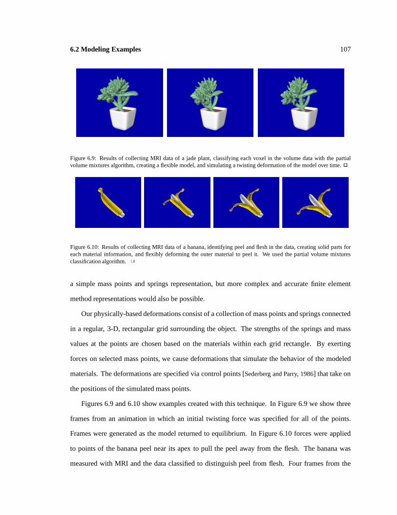
6.2 Modeling Examples 107
Figure 6.9: Results of collecting MRI data of a jade plant, classifying each voxel in the volume data with the partialvolume mixtures algorithm, creating a flexible model, and simulating a twisting deformation of the model over time. 2
Figure 6.10: Results of collecting MRI data of a banana, identifying peel and flesh in the data, creating solid parts foreach material information, and flexibly deforming the outer material to peel it. We used the partial volume mixturesclassification algorithm. 2
a simple mass points and springs representation, but more complex and accurate finite element
method representations would also be possible.
Our physically-based deformations consist of a collection of mass points and springs connected
in a regular, 3-D, rectangular grid surrounding the object. The strengths of the springs and mass
values at the points are chosen based on the materials within each grid rectangle. By exerting
forces on selected mass points, we cause deformations that simulate the behavior of the modeled
materials. The deformations are specified via control points [Sederberg and Parry, 1986] that take on
the positions of the simulated mass points.
Figures 6.9 and 6.10 show examples created with this technique. In Figure 6.9 we show three
frames from an animation in which an initial twisting force was specified for all of the points.
Frames were generated as the model returned to equilibrium. In Figure 6.10 forces were applied
to points of the banana peel near its apex to pull the peel away from the flesh. The banana was
measured with MRI and the data classified to distinguish peel from flesh. Four frames from the
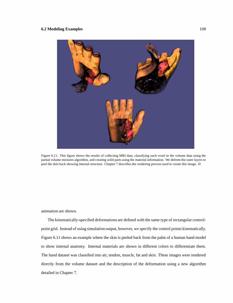
6.2 Modeling Examples 108
Figure 6.11: This figure shows the results of collecting MRI data, classifying each voxel in the volume data using thepartial volume mixtures algorithm, and creating solid parts using the material information. We deform the outer layers topeel the skin back showing internal structure. Chapter 7 describes the rendering process used to create this image. 2
animation are shown.
The kinematically-specified deformations are defined with the same type of rectangular control-
point grid. Instead of using simulation output, however, we specify the control points kinematically.
Figure 6.11 shows an example where the skin is peeled back from the palm of a human hand model
to show internal anatomy. Internal materials are shown in different colors to differentiate them.
The hand dataset was classified into air, tendon, muscle, fat and skin. These images were rendered
directly from the volume dataset and the description of the deformation using a new algorithm
detailed in Chapter 7.
6.3 Conclusion 109
6.3 Conclusion
Through a sequence of examples we have shown that classified MRI volume data can be used to
create both static and dynamic models. While the resolution of conventional MRI data is somewhat
less than that of surface measurement techniques, it is sufficient to create many types of models,
and the internal measurements available make dynamics more accurate for models with interior
structure.
By creating a series of geometric models we have determined a number of requirements for
the earlier steps in our computational framework. First, because real-world objects contain more
than one material, we need to be able to identify and separate the multiple different materials in
our sampled datasets. Isosurfaces do this in unclassified MRI data only for exactly two materials,
and only if the boundary between them is at a consistent and known value. Through classification
we can define isosurfaces for each material. Together the surfaces combine to represent all of the
material-material boundaries. Our classification process also provides a physical interpretation for
the data that defines a choice of isovalue for calculating a surface.
While many classification algorithms work well at identifying materials within regions of pure
materials, they do not produce accurate results where materials meet one another. Our investigations
have motivated the need for classification algorithms that are accurate at these boundaries. The
boundaries are where surface models are defined, and errors there cause artifacts in the extracted
models. Our new classification techniques reduce these artifacts significantly.
Third, there must be sufficient information in the collected data for our classification algorithms
to identify boundaries. We have translated this requirement into a contrast-to-noise goal in the
goal-based collection process.
Fourth, our model-extraction techniques find isosurfaces in continuous functions. If collected
data does not satisfy the Nyquist sampling theorem, then any continuous function that we reconstruct
from the samples will have aliasing and hence lead to artifacts in the extracted model.
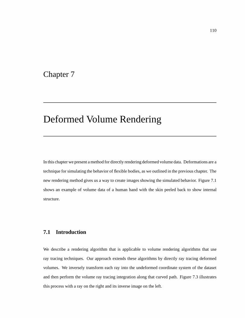
110
Chapter 7
Deformed Volume Rendering
In this chapter we present a method for directly rendering deformed volume data. Deformations are a
technique for simulating the behavior of flexible bodies, as we outlined in the previous chapter. The
new rendering method gives us a way to create images showing the simulated behavior. Figure 7.1
shows an example of volume data of a human hand with the skin peeled back to show internal
structure.
7.1 Introduction
We describe a rendering algorithm that is applicable to volume rendering algorithms that use
ray tracing techniques. Our approach extends these algorithms by directly ray tracing deformed
volumes. We inversely transform each ray into the undeformed coordinate system of the dataset
and then perform the volume ray tracing integration along that curved path. Figure 7.3 illustrates
this process with a ray on the right and its inverse image on the left.
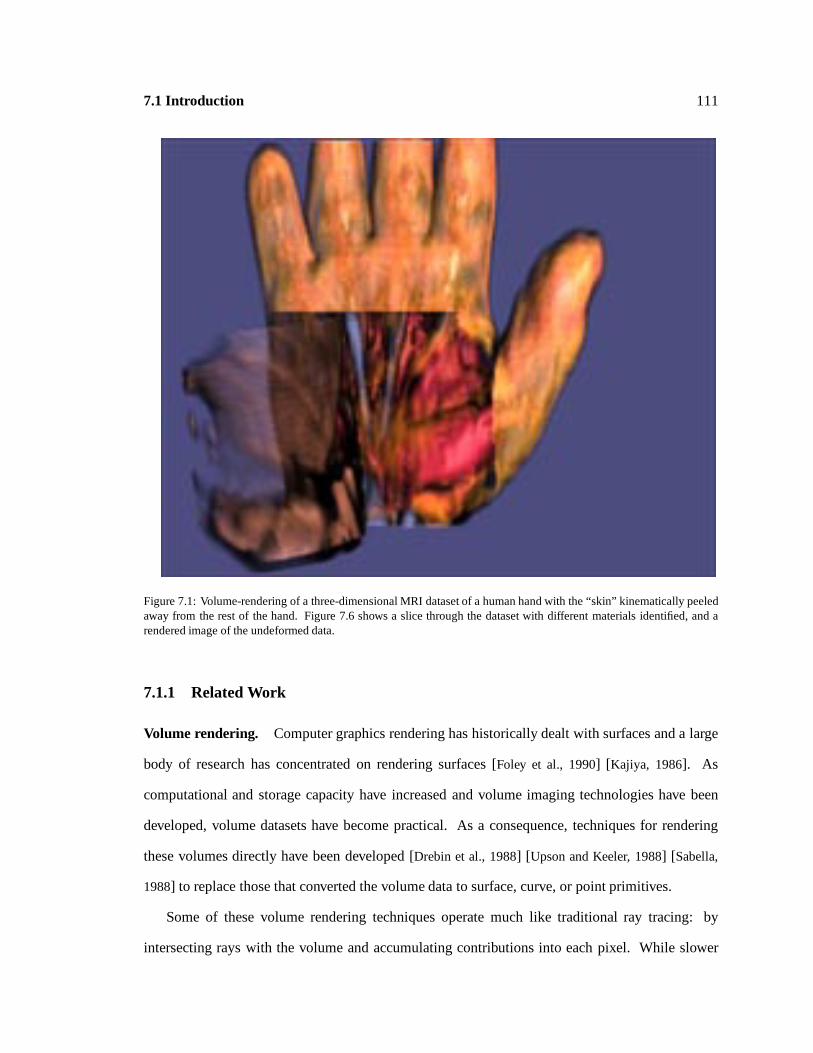
7.1 Introduction 111
Figure 7.1: Volume-rendering of a three-dimensional MRI dataset of a human hand with the “skin” kinematically peeledaway from the rest of the hand. Figure 7.6 shows a slice through the dataset with different materials identified, and arendered image of the undeformed data. 2
7.1.1 Related Work
Volume rendering. Computer graphics rendering has historically dealt with surfaces and a large
body of research has concentrated on rendering surfaces [Foley et al., 1990] [Kajiya, 1986]. As
computational and storage capacity have increased and volume imaging technologies have been
developed, volume datasets have become practical. As a consequence, techniques for rendering
these volumes directly have been developed [Drebin et al., 1988] [Upson and Keeler, 1988] [Sabella,
1988] to replace those that converted the volume data to surface, curve, or point primitives.
Some of these volume rendering techniques operate much like traditional ray tracing: by
intersecting rays with the volume and accumulating contributions into each pixel. While slower
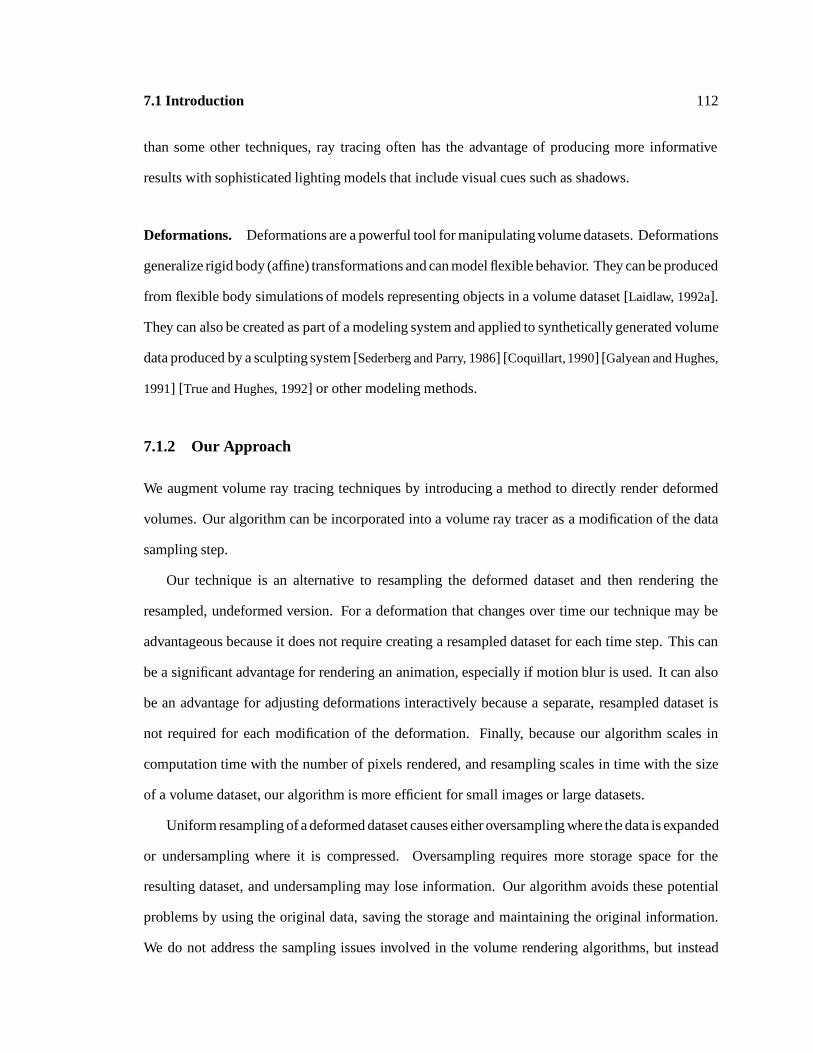
7.1 Introduction 112
than some other techniques, ray tracing often has the advantage of producing more informative
results with sophisticated lighting models that include visual cues such as shadows.
Deformations. Deformations are a powerful tool for manipulating volume datasets. Deformations
generalize rigid body (affine) transformations and can model flexible behavior. They can be produced
from flexible body simulations of models representing objects in a volume dataset [Laidlaw, 1992a].
They can also be created as part of a modeling system and applied to synthetically generated volume
data produced by a sculpting system [Sederberg and Parry, 1986] [Coquillart, 1990] [Galyean and Hughes,
1991] [True and Hughes, 1992] or other modeling methods.
7.1.2 Our Approach
We augment volume ray tracing techniques by introducing a method to directly render deformed
volumes. Our algorithm can be incorporated into a volume ray tracer as a modification of the data
sampling step.
Our technique is an alternative to resampling the deformed dataset and then rendering the
resampled, undeformed version. For a deformation that changes over time our technique may be
advantageous because it does not require creating a resampled dataset for each time step. This can
be a significant advantage for rendering an animation, especially if motion blur is used. It can also
be an advantage for adjusting deformations interactively because a separate, resampled dataset is
not required for each modification of the deformation. Finally, because our algorithm scales in
computation time with the number of pixels rendered, and resampling scales in time with the size
of a volume dataset, our algorithm is more efficient for small images or large datasets.
Uniform resampling of a deformed dataset causes either oversampling where the data is expanded
or undersampling where it is compressed. Oversampling requires more storage space for the
resulting dataset, and undersampling may lose information. Our algorithm avoids these potential
problems by using the original data, saving the storage and maintaining the original information.
We do not address the sampling issues involved in the volume rendering algorithms, but instead
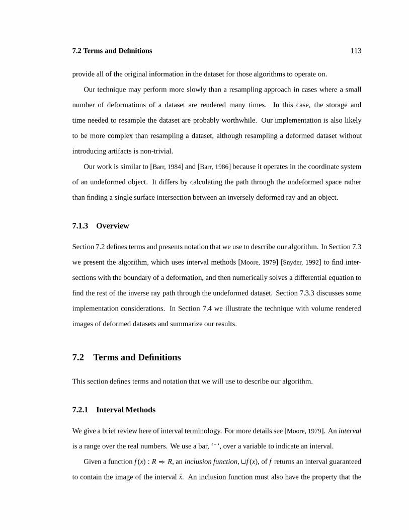
7.2 Terms and Definitions 113
provide all of the original information in the dataset for those algorithms to operate on.
Our technique may perform more slowly than a resampling approach in cases where a small
number of deformations of a dataset are rendered many times. In this case, the storage and
time needed to resample the dataset are probably worthwhile. Our implementation is also likely
to be more complex than resampling a dataset, although resampling a deformed dataset without
introducing artifacts is non-trivial.
Our work is similar to [Barr, 1984] and [Barr, 1986] because it operates in the coordinate system
of an undeformed object. It differs by calculating the path through the undeformed space rather
than finding a single surface intersection between an inversely deformed ray and an object.
7.1.3 Overview
Section 7.2 defines terms and presents notation that we use to describe our algorithm. In Section 7.3
we present the algorithm, which uses interval methods [Moore, 1979] [Snyder, 1992] to find inter-
sections with the boundary of a deformation, and then numerically solves a differential equation to
find the rest of the inverse ray path through the undeformed dataset. Section 7.3.3 discusses some
implementation considerations. In Section 7.4 we illustrate the technique with volume rendered
images of deformed datasets and summarize our results.
7.2 Terms and Definitions
This section defines terms and notation that we will use to describe our algorithm.
7.2.1 Interval Methods
We give a brief review here of interval terminology. For more details see [Moore, 1979]. An interval
is a range over the real numbers. We use a bar, ‘�’, over a variable to indicate an interval.
Given a function f (x) : R ) R, an inclusion function,2f (�x), of f returns an interval guaranteed
to contain the image of the interval �x. An inclusion function must also have the property that the

7.2 Terms and Definitions 114
output interval can be made arbitrarily small for some input interval around a given point. Inclusion
functions generalize in a straightforward way to higher dimensions.
Interval methods use inclusion functions for solving problems robustly [Snyder, 1992]. Inclusion
functions provide bounds for mathematical operations and so can be used to guarantee that some
property of an algorithm is true.
7.2.2 Volume Rendering
We model a dataset as a function
v(~xbody) : R3body ) Rm (7:1)
where m is the dimensionality of the dataset.
An affine transformation is often employed to place, scale and orient a dataset. We define this
as a function
~M(~xbody) : R3body ) R3
world (7:2)
Note that this can be implemented as a matrix operation using homogeneous coordinates [Foley
et al., 1990].
We define a ray as
r(s) : R ) R3world (7:3)
The inverse of the affine transformation applied to that ray gives another ray in the coordinate system
of the dataset
~P(s) = ~M�1(r(s)) (7:4)
We use the following volume rendering equation to model the operation of most ray tracing
volume renderers.
I(s) =Z s
0e�R s
0f (~P(^s);v(^s))d^sg(~P(s); v(s))ds (7:5)
where f (^s) and g(s) are functions that model light interacting with material at a point in space. See
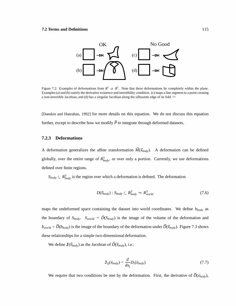
7.2 Terms and Definitions 115
(a)
(b)
(c)
(d)
OK No Good
Figure 7.2: Examples of deformations from R2) R2. Note that these deformations lie completely within the plane.
Examples (a) and (b) satisfy the derivative existence and invertibility condition. (c) maps a line segment to a point creatinga non-invertible Jacobian, and (d) has a singular Jacobian along the silhouette edge of its fold. 2
[Danskin and Hanrahan, 1992] for more details on this equation. We do not discuss this equation
further, except to describe how we modify ~P to integrate through deformed datasets.
7.2.3 Deformations
A deformation generalizes the affine transformation ~M(~xbody). A deformation can be defined
globally, over the entire range of R3body; or over only a portion. Currently, we use deformations
defined over finite regions.
Sbody � R3body is the region over which a deformation is defined. The deformation
D(~xbody) : Sbody � R3body ) R3
world (7:6)
maps the undeformed space containing the dataset into world coordinates. We define bbody as
the boundary of Sbody. Sworld = ~D(Sbody) is the image of the volume of the deformation and
bworld = ~D(bbody) is the image of the boundary of the deformation under ~D(~xbody). Figure 7.3 shows
these relationships for a simple two-dimensional deformation.
We define J(~xbody) as the Jacobian of ~D(~xbody), i.e.:
Jij(~xbody) =d
dxjDi(~xbody) (7:7)
We require that two conditions be met by the deformation. First, the derivative of ~D(~xbody),
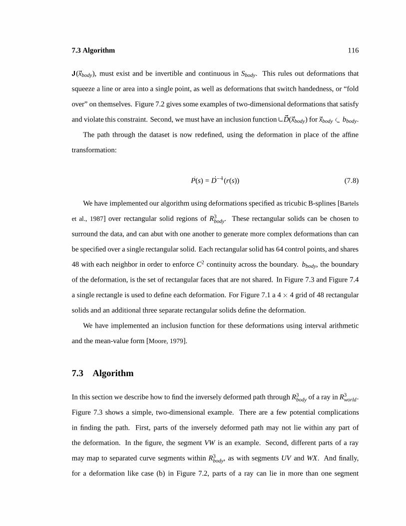
7.3 Algorithm 116
J(~xbody), must exist and be invertible and continuous in Sbody. This rules out deformations that
squeeze a line or area into a single point, as well as deformations that switch handedness, or “fold
over” on themselves. Figure 7.2 gives some examples of two-dimensional deformations that satisfy
and violate this constraint. Second, we must have an inclusion function2~D(~xbody) for~xbody � bbody.
The path through the dataset is now redefined, using the deformation in place of the affine
transformation:
~P(s) = ~D�1(r(s)) (7:8)
We have implemented our algorithm using deformations specified as tricubic B-splines [Bartels
et al., 1987] over rectangular solid regions of R3body. These rectangular solids can be chosen to
surround the data, and can abut with one another to generate more complex deformations than can
be specified over a single rectangular solid. Each rectangular solid has 64 control points, and shares
48 with each neighbor in order to enforce C2 continuity across the boundary. bbody, the boundary
of the deformation, is the set of rectangular faces that are not shared. In Figure 7.3 and Figure 7.4
a single rectangle is used to define each deformation. For Figure 7.1 a 4� 4 grid of 48 rectangular
solids and an additional three separate rectangular solids define the deformation.
We have implemented an inclusion function for these deformations using interval arithmetic
and the mean-value form [Moore, 1979].
7.3 Algorithm
In this section we describe how to find the inversely deformed path through R3body of a ray in R3
world.
Figure 7.3 shows a simple, two-dimensional example. There are a few potential complications
in finding the path. First, parts of the inversely deformed path may not lie within any part of
the deformation. In the figure, the segment VW is an example. Second, different parts of a ray
may map to separated curve segments within R3body, as with segments UV and WX. And finally,
for a deformation like case (b) in Figure 7.2, parts of a ray can lie in more than one segment
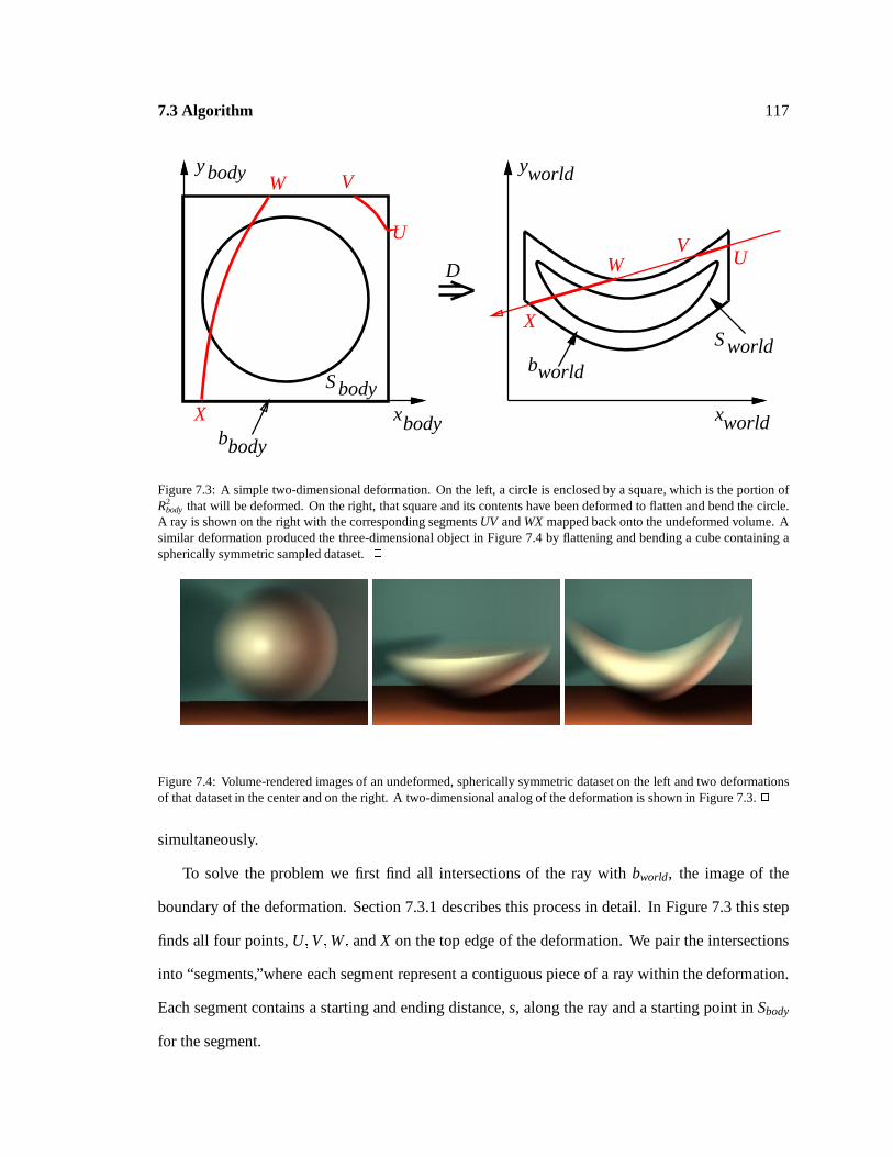
7.3 Algorithm 117
UV
W
X
xworld
S worldbworld
D
xbody
U
VW
X
S body
bbody
y body yworld
Figure 7.3: A simple two-dimensional deformation. On the left, a circle is enclosed by a square, which is the portion ofR2
body that will be deformed. On the right, that square and its contents have been deformed to flatten and bend the circle.A ray is shown on the right with the corresponding segments UV and WX mapped back onto the undeformed volume. Asimilar deformation produced the three-dimensional object in Figure 7.4 by flattening and bending a cube containing aspherically symmetric sampled dataset. 2
Figure 7.4: Volume-rendered images of an undeformed, spherically symmetric dataset on the left and two deformationsof that dataset in the center and on the right. A two-dimensional analog of the deformation is shown in Figure 7.3. 2
simultaneously.
To solve the problem we first find all intersections of the ray with bworld, the image of the
boundary of the deformation. Section 7.3.1 describes this process in detail. In Figure 7.3 this step
finds all four points, U;V ;W; and X on the top edge of the deformation. We pair the intersections
into “segments,”where each segment represent a contiguous piece of a ray within the deformation.
Each segment contains a starting and ending distance, s, along the ray and a starting point in Sbody
for the segment.
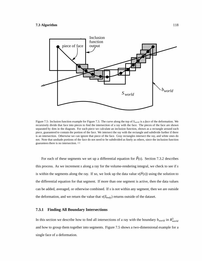
7.3 Algorithm 118
S worldbworld
Inclusionfunctionoutputpiece of face
Figure 7.5: Inclusion function example for Figure 7.3. The curve along the top of Sworld is a face of the deformation. Werecursively divide that face into pieces to find the intersection of a ray with the face. The pieces of the face are shownseparated by dots in the diagram. For each piece we calculate an inclusion function, shown as a rectangle around eachpiece, guaranteed to contain the portion of the face. We intersect the ray with the rectangle and subdivide further if thereis an intersection. Otherwise we can ignore that piece of the face. Gray rectangles intersect the ray, and white ones donot. Note that unshade portions of the face do not need to be subdivided as finely as others, since the inclusion functionguarantees there is no intersection. 2
For each of these segments we set up a differential equation for ~P(s). Section 7.3.2 describes
this process. As we increment s along a ray for the volume-rendering integral, we check to see if s
is within the segments along the ray. If so, we look up the data value v(~P(s)) using the solution to
the differential equation for that segment. If more than one segment is active, then the data values
can be added, averaged, or otherwise combined. If s is not within any segment, then we are outside
the deformation, and we return the value that v(~xbody) returns outside of the dataset.
7.3.1 Finding All Boundary Intersections
In this section we describe how to find all intersections of a ray with the boundary bworld in R3world
and how to group them together into segments. Figure 7.5 shows a two-dimensional example for a
single face of a deformation.

7.3 Algorithm 119
We use the inclusion function 2~D(�xbody) to find all intersections. We evaluate the inclusion
function for each rectangular face of the boundary in R3world . The interval result is a three-dimensional
interval in R3world. For example, 2~D([x0; x1]; [y1; y1]; [z0; z1]) returns an interval in R3
world containing
the image of the face where y = y1. If the ray ~r(s) intersects the interval in R3world, we save the
intersection and boundary information in a priority queue indexed by the nearest value of s within
the R3world interval.
Once all the faces that the ray might intersect are in the priority queue, we remove them one at
a time. If the current candidate is sufficiently small, we save it in a list of potential intersections.
If not, we subdivide it in half in each direction, repeat the interval evaluation for the smaller range,
and repeat the ray intersection test for the smaller R3world interval. The new, smaller intervals may
or may not intersect the ray, so we save the intersection and boundary information only for those
R3world intervals that do. Figure 7.5 shows an example of the lowest-level intervals that are tested by
this procedure. The large interval in the upper left is discarded early, because it does not overlap
the ray. The final list of potential intersections is represented by the shaded boxes.
We repeat until the priority queue is empty, and then construct segments from the list of
potential intersections. We are interested in pairing together each entrance with an exit, and we start
by identifying each potential intersection as one or the other. We use the surface normal in R3world
and compare it with the ray direction. For the y = y1 face,
~N(x; y1; z) =@~D@x
(x; y1; z)^ @~D@z
(x; y1; z) (7:9)
~N(x; y1; z) � rd < 0 ) entering (7:10)
and similarly for the other faces.
Each intersection can be represented by more than one potential intersection in the list because
the inclusion functions are always larger than the actual function values. Once we have subdivided
so that the size of the intervals is smaller than the error tolerance threshold of our renderer, we
coalesce potential intersections that are all entering or exiting and that have overlapping R3world
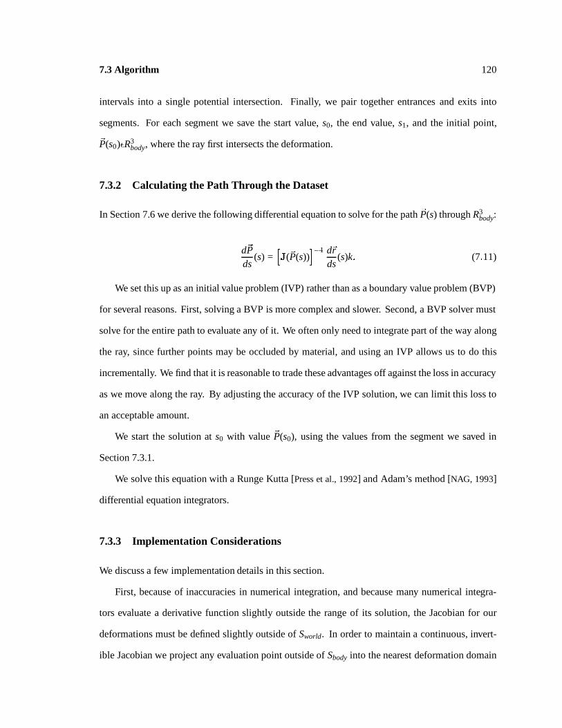
7.3 Algorithm 120
intervals into a single potential intersection. Finally, we pair together entrances and exits into
segments. For each segment we save the start value, s0, the end value, s1, and the initial point,
~P(s0)�R3body, where the ray first intersects the deformation.
7.3.2 Calculating the Path Through the Dataset
In Section 7.6 we derive the following differential equation to solve for the path ~P(s) through R3body:
d~Pds
(s) =hJ(~P(s))
i�1 d~rds
(s)k: (7:11)
We set this up as an initial value problem (IVP) rather than as a boundary value problem (BVP)
for several reasons. First, solving a BVP is more complex and slower. Second, a BVP solver must
solve for the entire path to evaluate any of it. We often only need to integrate part of the way along
the ray, since further points may be occluded by material, and using an IVP allows us to do this
incrementally. We find that it is reasonable to trade these advantages off against the loss in accuracy
as we move along the ray. By adjusting the accuracy of the IVP solution, we can limit this loss to
an acceptable amount.
We start the solution at s0 with value ~P(s0), using the values from the segment we saved in
Section 7.3.1.
We solve this equation with a Runge Kutta [Press et al., 1992] and Adam’s method [NAG, 1993]
differential equation integrators.
7.3.3 Implementation Considerations
We discuss a few implementation details in this section.
First, because of inaccuracies in numerical integration, and because many numerical integra-
tors evaluate a derivative function slightly outside the range of its solution, the Jacobian for our
deformations must be defined slightly outside of Sworld. In order to maintain a continuous, invert-
ible Jacobian we project any evaluation point outside of Sbody into the nearest deformation domain

7.3 Algorithm 121
Figure 7.6: Classified data, colored histogram, and image of undeformed hand dataset shown deformed in Figure 7.1.The top left image shows one slice from a three-dimensional MRI dataset of a human hand. At each spatial point we havetwo data values. The plot in the lower left shows a top view of the 2-dimensional histogram of that data, with MRI valuesalong the left and bottom axes and values for different materials given different colors. The slice has those colors appliedto it, with skin orange, muscle red, fat and bone marrow yellow/green, and tendon black. The right image shows the samedataset volume-rendered. 2
Figure 7.7: A photograph of a jade plant, a volume rendering of undeformed data collected from the jade plant, and avolume rendering of that data deformed. The right-hand image is one frame from those shown in Figure 6.9 2
boundary point and use the Jacobian value there.
Second, we have found that the interval evaluation for finding intersections is the most costly
part of our implementation. We have significantly increased performance by caching the interval
calculations for the first three levels of the subdivision hierarchy.
Third, our initial rays must start outside of a deformation in order to find their initial intersection
points. The interval methods could be extended to find an initial point within the deformation,but our
implementation does not do this. Rays created within a volume must start with “pseudo-entrance”
intersections for each segment active at the point the new ray was spawned. The intersection-finding
algorithm will then pair them up with exiting intersections to create segments for the new ray.
7.4 Results 122
7.4 Results
We have shown several examples of volume datasets directly rendered with deformations. Figure 7.1
shows MRI volume data classified to identify skin, fat, muscle, tendon, and bone. The skin is
deformed to peel it back from the other materials, showing the interior structure of the dataset.
Figure 7.6 shows a single slice through the dataset with materials identified by their colors, and
a rendering of the hand with no deformation. The dataset was classified using the partial volume
mixtures algorithm.
Figure 7.4 illustrates a rendering of simple deformations applied to a simulated MRI dataset of
a solid ball.
Figure 7.7 shows a photograph of a living jade plant, an undeformed rendering of MRI data
collected from the jade plant, and a deformed version of the jade plant rendered with our algorithm.
The deformation was calculated as one frame of an animation showing how a jade plant might move
(see Figure 6.9).
7.5 Conclusion
We have described an algorithm for directly ray tracing deformed volume data. The algorithm
inversely deforms each ray and traces its curved path through the undeformed data. We have shown
several examples of images rendered using our implementation.
There are several advantages to directly ray tracing deformed volumes. As an alternative to
creating a new regularly sampled dataset by resampling the deformed one, our technique provides
a more concise representation for a deformed volume. This conciseness is particularly useful for
multiple deformations, or for deformations that vary over time. The space savings is also a benefit
when rendering small images of large datasets, because it is proportional to the size of the dataset,
while the run-time cost is proportional to the size of the image. Our technique also avoids the
oversampling or undersampling that is implied by resampling a deformed dataset.
While the implementation increases rendering time in our volume ray tracer by a factor of two
7.6 Derivation of Deformed Path 123
to three, we have several avenues to explore for speeding the calculation. Because most of the cost
is in finding intersections, we propose implementing tighter inclusion functions, using an interval
Newton method to converge on a solution more quickly. We could also exploit coherence more in
the interval evaluations by adaptively caching them in addition to the static caching of the first three
subdivision levels.
7.6 Derivation of Deformed Path
We derive the differential equation in Section 7.3.2 here. The derivation is in Einstein Summation
Notation (ESN) [Blinn, 1992].
~P(s) = ~D�1(~r(s)) is a portion of the path in R3body. It is only defined where ~D�1(~r(s)). This is
where the ray is within Sworld. In those regions, by definition:
~Pi(s) =Z s
0
d~Pi
ds(s)ds + ~Pi(s0) (7:12)
Differentiating and rewriting the integrand using the definition of ~P and the chain rule,
d~Pi
ds(s) = (D�1)i;j(r(s))rj;s(s) (7:13)
Because we restrict the Jacobian of the deformation to be invertible at all points, the derivative of
the inverse deformation is the matrix inverse of the Jacobian of the deformation.
(D�1)i;j(~xworld) =�[J(~xbody)]
�1�
ij(7:14)
so Equation 7.13 becomes:

7.6 Derivation of Deformed Path 124
d~Pi
ds(s) =
�[J(P(s))]�1
�ij
rj;s(s) (7:15)
Note that the argument of J is the path location in R3body, P(s) and that we have a known initial
condition at Pi(s0).
125
Chapter 8
Conclusions and Future Work
This chapter summarizes our work and presents conclusions in the first section and then discusses
some future research directions that our work suggests may be fruitful.
8.1 Conclusions
We have addressed the problem of creating geometric models of real-world objects. This is a major
problem in computer graphics, and our results have applications in scientific research, education, and
entertainment. We have chosen to use MRI as our measurement modality because it is relatively
non-invasive, measures chemical properties of living subjects very well, and provides us with
measurements of internal structure.
We have presented a computational framework for creating geometric models and images from
MRI data. The framework consists of three main steps. The first is data collection; the second, tissue
classification; and the third, model-building and visualization. Within the stages of the framework
we have implemented a number of new algorithms that help to make models and images. We outline
8.1 Conclusions 126
the results of our new algorithms and the interactions between them in this section.
8.1.1 Goal-based Data Collection
The novel contributions of our new paradigm for choosing MRI collection parameters are in its
goal-based framework, in the choice of goals for the optimization procedure, and in the use of the
optimization step to steer the acquisition process during acquisitions. Our framework provides a
methodology for adding goals and new protocols to the set that we have implemented. The goals we
implement are motivated by our desire to distinguish adjacent materials sufficiently well to be able
to produce geometric models from the data. Many of the objectives are also generally applicable
to applications such as medical or biological imaging. These goals differ from other work in that
they do not find parameters yielding the most contrast or highest contrast-to-noise ratio, but rather
find parameters yielding sufficient contrast in the least amount of time. Any number of materials
can be specified by a user from low-resolution test datasets, and optimal collection parameters
are generated taking into account inherent machine limitations and fixed parameters such as field
of view and resolution. Finally, because values of the function we optimize are consistent from
protocol to protocol, we can compare them and choose the most appropriate protocol or combination,
independent of whether it produces scalar or vector-valued data.
8.1.2 Bayesian Classification
In the second stage of our computational framework we have developed a new methodology for
creating Bayesian classification algorithms from assumptions about the data-collection process.
Using the methodology we have created three new algorithms for classifying scalar and vector-
valued volume data. Our algorithms use a continuous reconstruction of the dataset and calculate
a continuous histogram of the data over regions representing each voxel. We derive intensity
probability density basis functions for both pure materials and mixtures of materials due to the
band-limiting effects of the data-collection process. Our classification process models histograms
over voxel regions using the material and mixture basis functions and uses a probabilistic approach

8.1 Conclusions 127
to fit the parameterized models to a histogram over each voxel.
In the partial volume mixtures approach, we modeled each voxel as a linear combination of pure
materials and mixtures of two materials. In the two boundary distance approaches we formulated
a more accurate model of voxels near boundaries between pure materials. The boundary distance
approaches classify voxels near boundaries more accurately, but at a larger computational cost.
We demonstrated the success of our techniques on simulated and real data by classifying datasets
of a human hand, human brains, and a bee, among others.
8.1.3 Model-Building and Visualization
Through a sequence of examples we have shown that classified MRI volume data can be used to
create both static and dynamic models. The level of detail in the models is somewhat less than
can be produced with surface scanning techniques, but the inclusion of internal structure adds
significantly more information to volume models and makes dynamic simulations more accurate.
With the internal structure, the behavior of different internal materials such as bone, muscle, and fat
can be taken into account.
We have also presented a new algorithm for directly rendering deformed volume data. This is
particularly useful for creating images of flexible-body simulations because it avoids the storage cost
and resampling difficulties inherent in creating a new sampled dataset for each step in a time-varying
deformation of volumetric data.
8.1.4 Interaction of Framework Stages
Throughout our investigations we have discovered that each stage of the framework mandates certain
conditions on the results of earlier stages. Starting with the model-extraction and visualization stage
of our pipeline, requirements feed back and influence earlier stages. This stage requires that its
input volume data identify different materials and the boundaries between them.
We infer from this requirement a need to classify the data that we collect, and to use an algorithm
that works well at boundaries between materials. Our new algorithms address this problem with

8.2 Extensions 128
more accuracy than previous methods.
The classification algorithms also place requirements on the data that we collect. The materials
and boundaries between them must be distinguishable in the data. We translate this into a contrast-
to-noise ratio goal within our goal-based data-collection process.
The model extraction and classification algorithms also require that we reconstruct a continuous
function from datasets, and so we require that the data we collect satisfy the Nyquist sampling
theorem.
The feedback of these requirements to the earlier stages of the framework helps tailor results
to the geometric modeling problem, providing us with tools that create more accurate geometric
models.
8.2 Extensions
Our work suggests a number of directions to consider for future research. We organize them here
in the context of our model-building framework.
8.2.1 Goal-based Data Collection
Within the goal-directed data-collection domain, we would like to extend the repertoire of collection
protocols and goals. Extending the protocols includes incorporating more collection parameters,
such as tip angle and sweep width (see Table 2.1), into the optimization process, as well as adding
to the list of protocols that can be supported. Using the technique on a wider variety of examples
will give us more feedback on its efficacy in providing us with data that will be useful for studying
anatomy and development.
Extending the goals includes formulating more goals for disparate uses of MRI data. The
imaging goal of achieving a particular contrast-to-noise ratio serves our classification algorithms
well, but might not be the best goal for other applications.
Our framework should also prove useful in choosing concentrations of MRI contrast agents to

8.2 Extensions 129
enhance particular materials. By modeling the effect of various concentrations of a contrast agent
on materials and incorporating that model into our goal-based framework, we can tailor the contrast
agent concentration to achieve better-quality data in less time.
The model of the MRI process we used is somewhat limited. It does not take into account the
mixing of multiple materials within a single voxel measurement, and would be somewhat difficult
to derive for a new protocol. Extending the model to include multiple materials might be a useful
project. The implementation of this should be straightforward,using the same Levenburg-Marquardt
non-linear parameter estimation technique.
We could also model the MRI process by numerically solving the Bloch equations [Bloch, 1948]
to predict data values as a function of protocol parameters. This would have the advantage of
working for an arbitrary protocol, as long as we can define the protocol in terms of a pulse-program
whose behavior is modeled well by the Bloch equations.
Through the numerical solution of the Bloch equations, it might be possible to generate new
pulse-programs via a genetic algorithm that evolved pulse programs and evaluated their effectiveness
via our objective function.
8.2.2 Artifacts in MRI Data
While we have addressed some of the artifacts that occur in MRI data, there are a number that
we have chosen to ignore. Different materials have different magnetic properties and boundaries
between them that cause susceptibility artifacts in MRI images. These artifacts occur primarily at
boundaries between materials or near accidental air bubbles, which tend to stick to these boundaries.
The artifacts are bright and dark patterns with a characteristic appearance within the data.
We could compensate for effects near boundaries with an extension to our boundary distance
classification algorithm, since information about the boundary is calculated as part of the algorithm.
The characteristic appearance of the artifacts caused by bubbles could be mitigated as a pre-
processing step or as part of the classification process.
Nonlinearities in the gradient coils used to encode spatial information in MRI data can lead to

8.2 Extensions 130
datasets with geometric distortions. We have not addressed geometric distortion in this work, except
to avoid its manifestations through judicious size and placement of the objects that we measure. In
principle, however, we should be able to compensate for these distortions through calibration of a
particular MRI machine. By understanding the errors in the underlying static magnetic field and
the gradients superimposed on it, we can model the geometric distortion created by those errors and
compensate for it.
8.2.3 Classification
Our classification algorithms have proven useful on the examples that we have applied them to, but
we would like to try them on more types of data in order to learn more about their characteristics and
breadth of applicability. Classifying data in an atlas of MRI datasets of a particular animal could
provide interesting results, both in the classified data itself and in feedback about the algorithms.
Our algorithms also should prove accurate at estimating volumes, especially for small regions where
errors near boundaries are significant compared to the entire volume.
There are a number of extensions to the classification algorithms we would like to suggest.
We have interpolated neighboring samples in classifying voxels, but would like to take further
advantage of this local geometric information. Incorporating the geometric information into the
prior probabilities for each voxel should help to avoid single misclassified voxels without losing
detail information that post-classification filtering processes destroy.
Another possible method for incorporating more geometric information into the classification
process would be to define a new type of voxel-info with that information and to derive a classification
algorithm based on that data. Combining the histogram voxel-info that we have implemented with
new voxel-info should produce better results than either alone.
Deriving new histogram basis functions would enable the algorithms to better classify data by
explicitly handling more situations. We would like to relax the assumption that objects consist of
regions of uniform materials. We can parameterize the histogram basis functions by the relative
content of each material, and anticipate a more continuous classification that would introduce fewer

8.2 Extensions 131
artifacts. We would also like to derive basis functions for geometries other than the pure and surface-
boundary cases that we have implemented. While these are the two most common geometries, edges
where three materials come together, points where four materials meet, and features like membranes
that are thinner than our sampling rate also occur and are important within the context of geometric
models.
Finally, two future directions for research include implementation of the boundary distance algo-
rithm to incorporate non-uniform response of materials within the sampled volume and acceleration
of our classification algorithms.
8.2.4 Model Building and Simulation
Our model-building and simulation work also implies a number of directions for augmentation. One
particularly interesting direction is in modeling and simulating the behavior of complicated flexible
bodies. This goal has inspired much of the work in this thesis, particularly the use of MRI data to
measure the internal structure of objects in addition to their external structure.
Future research could include a testbed for flexible-body simulations that incorporates new types
of constraints for sliding flexible bodies over one another without interpenetration and for making
structural connections between both flexible and rigid bodies. This type of simulation environment
would provide a predictive tool with medical, and scientific applications, and could be used for
entertainment purposes as well.
8.2.5 Volume Rendering
Volume rendering is a relatively new technique and holds a lot of promise for generating images
with visual information and cues that can improve understanding of the objects being rendered.
New techniques that generate different types of images through new, more general models of light
propagation through materials have solid research potential. Textures and translucency within
volumes of materials hold promise in generating these new looks.

8.3 Summary 132
8.3 Summary
Our work on a computational framework for creating geometric models from MRI volume data has
demonstrated the utility of the framework, led to a number of algorithmic results, and indicated
many avenues for future research.
133
Bibliography
[Baraff and Witkin, 1992] Baraff, D. and Witkin, A. (1992). Dynamic simulation of non-penetrating
flexible bodies. In Catmull, E. E., editor, Computer Graphics (SIGGRAPH ’92 Proceedings),
volume 26, pages 303–308.
[Barr, 1984] Barr, A. H. (1984). Global and local deformations of solid primitives. In Christiansen,
H., editor, Computer Graphics (SIGGRAPH ’84 Proceedings), volume 18, pages 21–30.
[Barr, 1986] Barr, A. H. (1986). Ray tracing deformed surfaces. In Evans, D. C. and Athay, R. J.,
editors, Computer Graphics (SIGGRAPH ’86 Proceedings), volume 20, pages 287–296.
[Bartels et al., 1987] Bartels, R., Beatty, J., and Barsky, B. (1987). An Introduction to Splines for
Use in Computer Graphics and Geometric Modeling. Morgan Kaufmann Publishers, Palo Alto,
CA.
[Blinn, 1992] Blinn, J. F. (1992). Uppers and downers. IEEE Computer Graphics and Applications,
12(3).
[Bloch, 1948] Bloch, F. (1948). Physical Review, 70.
[Choi et al., 1991] Choi, H. S., Haynor, D. R., and Kim, Y. M. (1991). Partial volume tissue
classification of multichannel magnetic resonance images - a mixel model. IEEE Transactions
on Medical Images, 10(3):395–407.
Bibliography 134
[Clarke et al., 1995] Clarke, L. P., Velthuizen, R. P., Camacho, M. A., Neine, J. J., Vaidyanathan,
M., Hall, L. O., Thatcher, R. W., and Silbiger, M. L. (1995). Mri segmentation: Methods and
applications. Magnetic Resonance Imaging, 13(3):343–368.
[Cline et al., 1990] Cline, H. E., Lorensen, W. E., Kikinis, R., and Jolesz, F. (1990). Three-
dimensional segmentation of mr images of the head using probability and connectivity. Journal
of Computer Assisted Tomography, 14(6):1037–1045.
[Coquillart, 1990] Coquillart, S. (1990). Extended free-form deformation: A sculpturing tool for 3D
geometric modeling. In Baskett, F., editor, Computer Graphics (SIGGRAPH ’90 Proceedings),
volume 24, pages 187–196.
[Danskin and Hanrahan, 1992] Danskin, J. and Hanrahan, P. (1992). Fast algorithms for volume ray
tracing. 1992 Workshop on Volume Visualization, pages 91–98.
[Drebin et al., 1988] Drebin, R. A., Carpenter, L., and Hanrahan, P. (1988). Volume rendering. In
Dill, J., editor, Computer Graphics (SIGGRAPH ’88 Proceedings), volume 22, pages 65–74.
[Dreher and Bornert, 1988] Dreher, W. and Bornert, P. (1988). Pulse sequence and parameter choice
in nmr imaging as a problem of constrained multidimensional nonlinear optimization. Magnetic
Resonance in Medicine, 8:16–24.
[Duda and Hart, 1973] Duda, R. P. and Hart, P. E. (1973). Pattern Classification and Scene Analysis.
John Wiley and Sons, New York.
[Dufour et al., 1993] Dufour, I., Bittoun, J., Idy-Peretti, I., Jolivet, O., Darrasse, L., and Paola, R. D.
(1993). Implementation and optimization by the simplex method of a 3d double echo sequence
in steady-state free precession. Magnetic Resonance Imaging, 11:87–93.
[Epstein et al., 1994] Epstein, F. H., III, J. P. M., and Brookeman, J. R. (1994). Optimization of
parameter values for complex pulse sequences by simulated annealing: Application to 3d mp-
rage imaging of the brain. Magnetic Resonance in Medicine, 31(2):164–177.
Bibliography 135
[Farrar and Becker, 1971] Farrar, T. C. and Becker, E. D. (1971). Pulse and Fourier Transform NMR
Introduction to Theory and Methods. The Bloch Equations. Academic Press, New York.
[Fleischer et al., 1995] Fleischer, K., Laidlaw, D., Currin, B., and Barr, A. H. (1995). Cellular texture
generation. Proceedings of Siggraph ’95, Los Angeles, CA. to appear.
[Foley et al., 1990] Foley, J. D., van Dam, A., Feiner, S. K., and Hughes, J. F. (1990). Computer
Graphics: Principles and Practices (2nd Edition). Addison Wesley.
[Fox and Henson, 1986] Fox, R. A. and Henson, P. W. (1986). A general method for optimizing
tissue discrimination in magnetic resonance imaging. Medical Physics, 13(5):635–643.
[Galyean and Hughes, 1991] Galyean, T. A. and Hughes, J. F. (1991). Sculpting: An interactive
volumetric modeling technique. In Sederberg, T. W., editor, Computer Graphics (SIGGRAPH
’91 Proceedings), volume 25, pages 267–274.
[Ghosh et al., 1995] Ghosh, P. R., Laidlaw, D. H., Fleischer, K. W., Barr, A. H., and Jacobs, R. E.
(1995). Pure phase-encoded mri and classification of solids. IEEE Transactions on Medical
Imaging, 14(3). (in press).
[Gravina and Cory, 1994] Gravina, S. and Cory, D. G. (1994). Sensitivity and resolution of constant-
time imaging. J. Magn. Reson., Series B, 104:53–61.
[Hendrick et al., 1984] Hendrick, R. E., Nelson, T. R., and Hendee, W. R. (1984). Optimizing tissue
contrast in magnetic resonance imaging. Magnetic Resonance Imaging, 2:193–204.
[Kajiya, 1986] Kajiya, J. T. (1986). The rendering equation. In Evans, D. C. and Athay, R. J.,
editors, Computer Graphics (SIGGRAPH ’86 Proceedings), volume 20, pages 143–150.
[Kanal and Wehrli, 1986] Kanal, E. and Wehrli, F. (1986). Principles, Methodology and Applications
of Biomedical Magnetic Resonance Imaging, chapter 2. VCH Publishers.
[Laidlaw, 1992a] Laidlaw, D. H. (1992a). Material classification of magnetic resonance volume data.
Technical Report CS-TR-92-21, Caltech.

Bibliography 136
[Laidlaw, 1992b] Laidlaw, D. H. (1992b). Tissue classification of magnetic resonance volume data.
Master’s project, California Institute of Technology.
[Levoy, 1988] Levoy, M. (1988). Display of surfaces from volume data. IEEE Computer Graphics
and Applications, 8(3):29–37.
[Loredo, 1989] Loredo, T. J. (1989). From laplace to supernova sn1987a: Bayesian inference in
astrophysics. In Fougere, P., editor, Maximum Entropy and Bayesian Methods. Kluwer Academic
Publishers, Denmark.
[Lorensen and Cline, 1987] Lorensen, W. E. and Cline, H. E. (1987). Marching cubes: A high
resolution 3D surface construction algorithm. In Stone, M. C., editor, Computer Graphics
(SIGGRAPH ’87 Proceedings), volume 21, pages 163–169.
[Mitchell et al., 1984] Mitchell, M. R., Conturo, T. E., Gruber, T. J., and Jones, J. P. (1984). Two
computer models for selection of optimal magnetic resonance imaging (mri) pulse sequence
timing. Investigative Radiology, 19(5).
[Moore, 1979] Moore, R. E. (1979). Methods and Applications of Interval Analysis. SIAM, Philadel-
phia, Pennsylvania.
[NAG, 1993] NAG (1993). NAG Fortran Library. Numerical Algorithms Group, 1400 Opus Place,
Suite 200, Downers Grove, Illinois 60515.
[Oppenheim et al., 1983] Oppenheim, A. V., Willsky, A. S., and Young, I. T. (1983). Signals and
Systems. Prentice-Hall, Inc., New Jersey.
[Pelc, 1993] Pelc, N. J. (1993). Optimization of flip angle for t1 dependent contrast in mri. Magnetic
Resonance in Medicine, 29(5):695–699.
[Platt and Barr, 1988] Platt, J. C. and Barr, A. H. (1988). Constraint methods for flexible models. In
Dill, J., editor, Computer Graphics (SIGGRAPH ’88 Proceedings), volume 22, pages 279–288.
Bibliography 137
[Press et al., 1992] Press, W. H., Teukolsky, S. A., Vetterling, W. T., and Flannery, B. P. (1992).
Numerical Recipes in C: The Art of Scientific Computing. Cambridge University Press, New
York, New York, second edition.
[Rosen et al., 1984] Rosen, B. R., Pykett, I. L., and Brady, T. J. (1984). Spin lattice relaxation time
measurements in two-dimensional nuclear magnetic resonance imaging: Corrections for plane
selection and pulse sequence. Journal of Computer Assisted Tomography, 8(6):195–199.
[Sabella, 1988] Sabella, P. (1988). A rendering algorithm for visualizing 3D scalar fields. In Dill,
J., editor, Computer Graphics (SIGGRAPH ’88 Proceedings), volume 22, pages 51–58.
[Sederberg and Parry, 1986] Sederberg, T. W. and Parry, S. R. (1986). Free-form deformation of solid
geometric models. In Evans, D. C. and Athay, R. J., editors, Computer Graphics (SIGGRAPH
’86 Proceedings), volume 20, pages 151–160.
[Snyder, 1992] Snyder, J. M. (1992). Interval analysis for computer graphics. In Catmull, E. E.,
editor, Computer Graphics (SIGGRAPH ’92 Proceedings), volume 26, pages 121–130.
[True and Hughes, 1992] True, T. J. and Hughes, J. F. (1992). Volume warping. In Proceedings
Visualization ’92, pages 308–315. IEEE Computer Society Press.
[Turk and Levoy, 1994] Turk, G. and Levoy, M. (1994). Zippered polygon meshes from range images.
In Glassner, A., editor, Proceedings of SIGGRAPH ’94 (Orlando, Florida, July 24–29, 1994),
Computer Graphics Proceedings, Annual Conference Series, pages 311–318. ACM SIGGRAPH,
ACM Press. ISBN 0-89791-667-0.
[Upson et al., 1989] Upson, C., Faulhaber, Jr., T., Kamins, D., Laidlaw, D., Schlegel, D., Vroom, J.,
Gurwitz, R., and van Dam, A. (1989). The application visualization system: A computational
environment for scientific visualization. IEEE Computer Graphics and Applications, 9(4):30–42.
[Upson and Keeler, 1988] Upson, C. and Keeler, M. (1988). VBUFFER: Visible volume rendering.
In Dill, J., editor, Computer Graphics (SIGGRAPH ’88 Proceedings), volume 22, pages 59–64.

Bibliography 138
[Vannier et al., 1985] Vannier, M. W., Butterfield, R. L., Jordan, D., Murphy, W. A., Levitt, R. G., and
Gado, M. (1985). Multispectral analysis of magnetic resonance images. Radiology, 154:221–224.
[Vannier et al., 1988] Vannier, M. W., Speidel, C. M., and Rickman, D. L. (1988). Magnetic resonance
imaging multispectral tissue classification. In Proc. Neural Information Processing Systems
(NIPS).
[Weil, 1986] Weil, J. (1986). The synthesis of cloth objects. In Evans, D. C. and Athay, R. J., editors,
Computer Graphics (SIGGRAPH ’86 Proceedings), volume 20, pages 49–54.