Geometric Constraint Solving in Parametric CAD

Bernhard Bettig∗ Christoph M. Hoffmann†

March 9, 2011

Abstract

With parametric Computer-Aided Design (CAD) software, designers cancreate geometric models that are easily updated (within limits) by modify-ing the values of controlling parameters. These numeric and non-numericparameters control the geometry in two ways:

(i) parametric operations, and

(ii) geometric constraint solving.

This paper examines the advances over the last decade in the represen-tation of parametric operations and of solving geometric constraint prob-lems. An extensive literature has grown up surrounding geometric con-straint solving and there has been substantial progress in the types ofobjects and constraints that can be handled robustly. Yet parametricoperations have remained largely within the same conceptualization andbegin to limit the flexibility of CAD systems, and so they still do not alignwell with a systematic design process.

Keywords: computer-aided design, parametric CAD, geometric constraints,geometric constraint solving, variational solvers, declarative constraints.

1 Introduction

Parametric Computer-Aided Design (CAD) software is used pervasively in thedesign and manufacture of modern-day mechanical products. In parametricCAD, designers define the size, shape and positions of geometric features andassembly components in terms of numerical and non-numerical parameters. Bychanging parameter values a design can be easily modified, within limits.

Two computational mechanisms, intertwined in current parametric CADsoftware, are used to control the geometry from input parameters:

∗Department of Mechanical Engineering, West Virginia University Institute of Technology,WV 25136; Bernhard.Bettig@mail.wvu.edu

†Department of Computer Science, Purdue University, West Lafayette, IN 47907;cmh@cs.purdue.edu

1

• Parametric operations, such as extrude and unite, which construct geomet-ric objects that satisfy implied constraints imposed when the user selectsthe operation and its inputs, and

• Geometric constraint solving, which repositions and scales geometric ob-jects in sketches and assemblies so that they satisfy constraints that areexplicitly imposed on them by the user.

This paper surveys the state of the art in parametric operations and geometricconstraint solving technology. It describes the state of the art a decade ago, aswell as advances that have occurred since then.

The paper first addresses, in Section 2, the technical challenges and advancesrelated to parametric operations in CAD, and explains how geometric constraintsolving fits with parametric CAD. Then the bulk of the paper addresses advancesin geometric constraint solving techniques, which are discussed in two majorsections:

• In Section 3, a broad range of approaches to constraint solving is dis-cussed. Over the years, many different approaches have been reported inthe literature, and this section sketches them briefly.

• To-date, the dominant approach to constraint solving is based on a con-straint graph analysis that formulates a solution plan, followed by a solverthat, usually recursively, elaborates the plan and computes a solution.This material is developed in Section 4.

Section 5 provides a summarizing discussion with some conclusions.The scope of the paper is limited to the computation of the size, shape and

placement of geometric objects including points, curves (e.g., straight lines, arcs,conics, and freeform), and surfaces (e.g., planar, cylindrical, conical, spherical,and freeform) as controlled through implicitly or explicitly-imposed geometricconstraints. The constraints can be dimensional, relating CAD parameters toradius, distance and angle, and they can be geometric, positing perpendicular-ity, concentricity, tangency, and so on. The problems can be posed in 2D or 3Dspace. The paper does not address the less centrally related subjects of geomet-ric topology, feature semantics, knowledge-based engineering, or optimization.

2 Parametric Operations in CAD

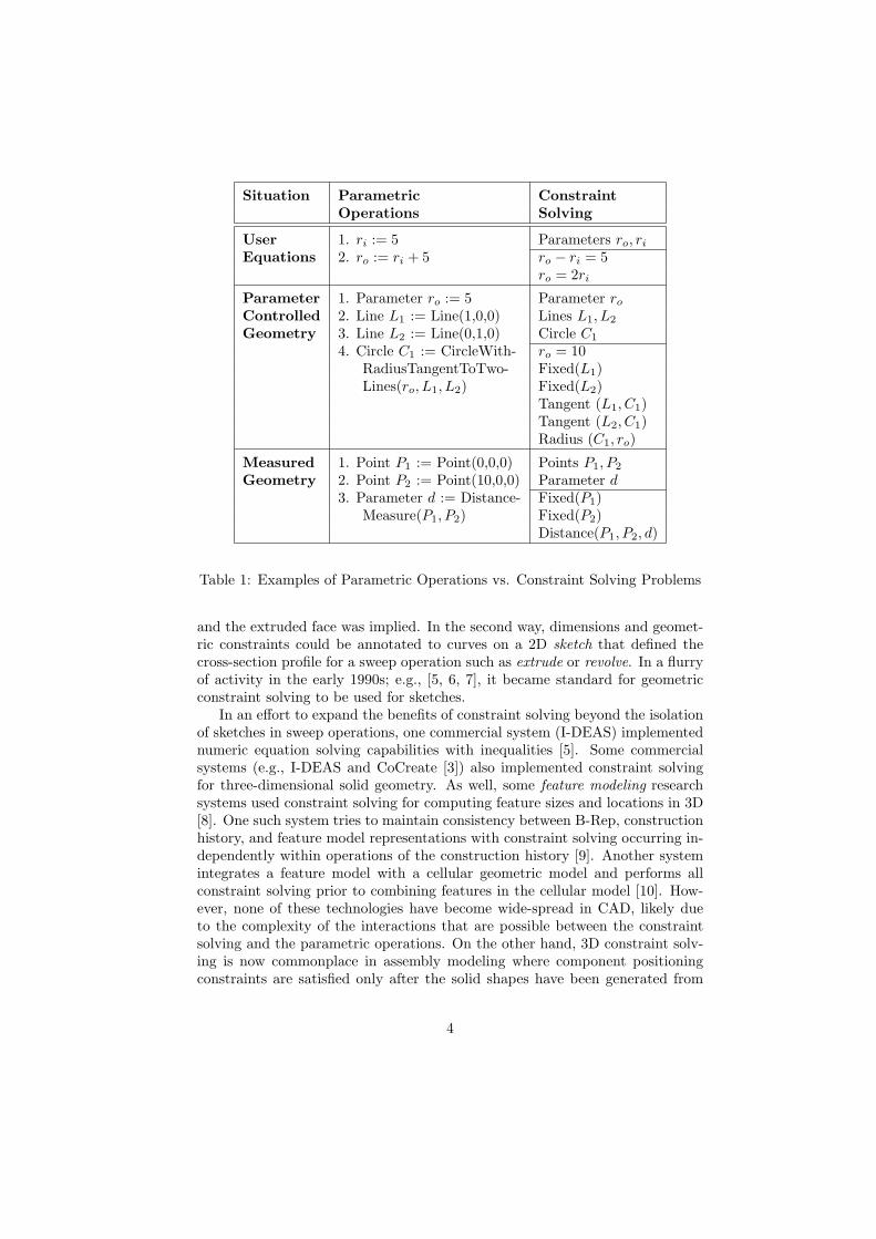
Parametric operations are created when a designer uses solid modeling opera-tions such as extrude, unite, and blend. The parametric operations are recordedas a sequence (or tree) of construction steps in a construction history that canbe controlled by the user. Parameters, such as the radius for a blend operation,occur as inputs to the operations. If the value of a parameter is changed, theconstruction history is re-executed and the updated geometry is constructed;e.g., [1]. As shown by the examples in Table 1, parametric operations mayinclude:

2

(i) user equations—controlling parameters from other parameters;

(ii) parameter controlled geometry—controlling geometry from parametersand other geometry; and

(iii) measured geometry—controlling parameters from geometric computations.

Variations of these operations may involve other types of parameters (e.g.,logical, enumerated, text string) and other geometric objects (e.g., completesketches, datums, solids), however, the salient point is that there is a fixed di-rectional dependency between the input entities on the right-hand-side of theassignment operations and the output entities on the left-hand-side. Therefore,while the parametric operation conceptualization lends itself to the provision ofcomputations with diverse kinds of geometric objects and (implied) constraints,the fixed directional dependency makes it necessary for users to plan aheadhow the features of the model should be controlled and may require manuallyuncoupling relationships that would otherwise give rise to cyclic dependencies.This conceptualization contrasts with the constraint solving conceptualizationin which there are no such fixed directional dependencies. Users introduce pa-rameters and geometric objects first and then annotate them with constraints,which are then satisfied through constraint solving computations. Advances inparametric operations technology relate to improvements in the types and ro-bustness of parametric operations themselves and to improvements in dealingwith the inflexibility of the fixed directional dependencies.

2.1 Developments Until 2000

The earliest parametric CAD system dates from the 1970s; [2]. It used a dualrepresentation, describing solids both in Constructive Solid Geometry (CSG)and in Boundary-Representation (B-Rep). In this dual representation, the solidmodel is represented as a binary tree in which the leaves are primitive shapessuch as blocks and cylinders, and the branches are Boolean operations such asUnite, Intersect, and Subtract. Each primitive can be thought of as a parametricoperation with input parameters defining size and position. The output is thenthe shape of the primitive as a B-Rep. Boolean operations take selected B-Repshapes as input and output the resulting B-Rep shape. The CSG tree provideda very basic construction history.

The first parametric CAD system, in the sense as it is understood today, isPro-Engineer, released by Parametric Technology Corporation in the late 1980s;[3]. In this CAD system the sizes and positions of geometric objects could bedirectly related to each other [4]. Thus if the user changed the value of a dimen-sion between geometric objects, or moved a geometric object, this could initiateother geometric objects to be moved automatically. Dimensions and geometricconstraints appeared in parametric operations in two ways. In the first way, di-mensions appeared as inputs to parametric operations and specific constraintswere implied. For example, in an extrude operation an input dimension con-trolled the length of the extrusion and perpendicularity between the side faces

3

Situation Parametric ConstraintOperations Solving

User 1. ri := 5 Parameters ro, riEquations 2. ro := ri + 5 ro − ri = 5

ro = 2ri

Parameter 1. Parameter ro := 5 Parameter roControlled 2. Line L1 := Line(1,0,0) Lines L1, L2

Geometry 3. Line L2 := Line(0,1,0) Circle C1

4. Circle C1 := CircleWith- ro = 10RadiusTangentToTwo- Fixed(L1)Lines(ro, L1, L2) Fixed(L2)

Tangent (L1, C1)Tangent (L2, C1)Radius (C1, ro)

Measured 1. Point P1 := Point(0,0,0) Points P1, P2

Geometry 2. Point P2 := Point(10,0,0) Parameter d3. Parameter d := Distance- Fixed(P1)

Measure(P1, P2) Fixed(P2)Distance(P1, P2, d)

Table 1: Examples of Parametric Operations vs. Constraint Solving Problems

and the extruded face was implied. In the second way, dimensions and geomet-ric constraints could be annotated to curves on a 2D sketch that defined thecross-section profile for a sweep operation such as extrude or revolve. In a flurryof activity in the early 1990s; e.g., [5, 6, 7], it became standard for geometricconstraint solving to be used for sketches.

In an effort to expand the benefits of constraint solving beyond the isolationof sketches in sweep operations, one commercial system (I-DEAS) implementednumeric equation solving capabilities with inequalities [5]. Some commercialsystems (e.g., I-DEAS and CoCreate [3]) also implemented constraint solvingfor three-dimensional solid geometry. As well, some feature modeling researchsystems used constraint solving for computing feature sizes and locations in 3D[8]. One such system tries to maintain consistency between B-Rep, constructionhistory, and feature model representations with constraint solving occurring in-dependently within operations of the construction history [9]. Another systemintegrates a feature model with a cellular geometric model and performs allconstraint solving prior to combining features in the cellular model [10]. How-ever, none of these technologies have become wide-spread in CAD, likely dueto the complexity of the interactions that are possible between the constraintsolving and the parametric operations. On the other hand, 3D constraint solv-ing is now commonplace in assembly modeling where component positioningconstraints are satisfied only after the solid shapes have been generated from

4

Figure 1: Blended edge (a) small radius (b) error condition (c) tangency removed

the parametric modeling operations.Improvements in parametric operations themselves have primarily been in

their robustness and variety; for example, edge blend operations that used to failwhen the radius of the blend was greater than the width of the tangent face nowautomatically forgo the tangency requirement in order to obtain a solution (asshown in Figure 1); see also [11]. However, the overall framework of parametricoperations has stayed the same. Some applications have made interesting useof this framework, for example for parametric design optimization in which thedimensional parameters are manipulated by an optimization algorithm in orderto satisfy a geometric goal (e.g., desired volume) or structural goal (e.g., desiredstress from imposed loads; [12]).

2.2 Developments Since 2000

The emphasis of the last decade has been on mitigating the rigidity inherentin parametric CAD owing to the parametric operations [13, 14]. For example,it should be possible to simply grab a face and drag it to where it should be.Instead, the designer must find the controlling operation in the constructionhistory, and within that operation find the controlling parameter. This couldbe for example a dimension in a sketch or the length of an extrusion. Chang-ing the value of the parameter may then have unintended side-effects in otheroperations; e.g., [1]. To overcome this inflexibility, a variety of hybrid mod-eling systems have been developed by vendors and researchers that combineparametric and direct-manipulation interfaces; [15, 16, 17]. In these systemsit is possible to reposition faces, scale the sizes of features or even twist fea-tures. Unfortunately, these systems implement the direct modeling interactionsas transformation operations that are simply added to the construction his-tory as additional parametric operations. For example, using the Move Faceoperation in Siemens PLM NX 7.5 Synchronous Technology [18] the user canselect a side face on a parametrically-defined solid and translate it interactivelyin the graphics display to make the shape 2 mm wider. The magnitude anddirection of the translation is recorded in a new parametric operation and theprevious operations in the construction history are maintained exactly as before.

5

If the dimension for the original width is changed, the construction history isreplayed, including the Move Face operation, which keeps the width 2 mm widerthan specified. Thus meaningful parametric control is lost. Another approachto resolve the inflexibility problem has been to treat some parameters as softparameters and assign intervals [19] or set membership [20].

The limitations inherent with using parametric operations as a basis fordesign software are discussed by Bettig et al. [13]. They find that the searchfor design solutions when following a systematic design process is impeded byparametric operations because:

◦ Designs from parametric operations are implicitly fully constrained. Ingeneral, it is not clear which input parameters are controlled by require-ments and which parameters can be tweaked. As well, some of the con-straints implied by an operation may be superfluous with respect to thedesign intent or design requirements.

◦ Parametric operations are designed to output a unique solution. Oftenthere are multiple mathematical solutions that should be explored.

◦ Parametric operations inherently bundle all implied constraints control-ling an object into a single operation. Thus it is impossible to imposeconstraints from multiple sources onto a single object without manuallycombining them into one operation. It is also impossible to add furthercontrols on an object once the object has been defined through a paramet-ric operation. As well, coupled constraints must be manually uncoupled.

◦ The constraints or design intent implicit in a parametric operation can beviolated by the parametric operations that follow it.

Future design software is proposed that does not rely on parametric operations,however, it is clear that parametric operations will continue to be used for thenear future.

3 Major Approaches to Geometric ConstraintSolving

The literature on geometric constraint solving often abstracts the problem asfollows:

Given a set of geometric objects, such as points, lines and circles;given a set of geometric and dimensional constraints, such as dis-tance, tangency, perpendicularity etc.; and given an ambient space,usually the Euclidean plane; assign coordinates to the geometric ob-jects such that the constraints are satisfied, or report that no suchassignment has been found.

6

The competence of the solver is related to the report that no solution has beenfound: If no solution exists in that case, the solver is fully competent. Ontheoretical grounds constraint solving is doubly exponential, so that in practicewe settle for partial competence as long as the solver finds a solution for mostof the problems arising in an application area, in acceptable time and space.

The main approaches to solving constraint problems are graph-based, logic-based, algebraic, and theorem prover-based. See also [21] that informs some ofthe material in this section.

3.1 Developments Until 2000

3.1.1 Graph-Based Approaches

In the graph-based approach, the constraint problem is translated into a labeledgraph, the constraint graph with vertices representing the geometric objectsthat are constrained, and edges representing the constraints themselves. Wedistinguish three main strands: the constructive approach, the degree of freedomtechniques and propagation methods.

Constructive Approaches

In this approach, the constraint graph is decomposed and recombined to ex-tract basic construction steps that must be solved. A second phase elaboratesthese steps, employing algebraic and/or numerical methods. This approach hasbecome dominant and will be discussed in depth in the next section.

Degrees of Freedom Analysis

The graph vertices are labeled with the number of degrees of freedom of therepresented geometric object. In 2D, a point would have 2 degrees of freedom,a circle 3. Each graph edge is labeled by the degrees of freedom canceled by therepresented constraints. If the incident vertices are points in 2D, for instance, anincidence constraint cancels 2, a distance constraint cancels 1 degree of freedom.This graph is analyzed for a solution strategy.

Kramer [22, 23] uses this approach to analyze and solve certain mechanisms.A symbolic solution method is derived using rules that have a geometric mean-ing. In [23], Kramer proves correctness of his method by establishing that thealgorithm can be understood as a canonical rewrite system. Hsu [24] solves theconstraint problem in two phases, generating first a symbolic rules representa-tion, followed by elaborating those rules by solving them. If geometric reasoningfails, a numerical solution is attempted.

Latham et al., [25], decompose the graph into minimal connected compo-nents they call balanced sets. If a balanced set is in a predefined set of patterns,then the subproblem is solved by a geometric construction, otherwise a numericsolution is attempted. This method also deals with symbolic constraints andidentifies under- and overconstrained problems. Overconstrained problems areapproached by prioritizing the given constraints.

7

Propagation Approaches

These methods encode the constraint problem by a graph in which the verticesrepresent variables and equations, and edges are labeled with occurrences ofvariables in equations. Propagation seeks to orient the graph edges such thatall incident edges to an equation vertex are incoming edges except for one. Ifthis succeeds, then the equation system has been triangularized. Orientationalgorithms include degree-of-freedom propagation and propagation of knownvalues; e.g., [26, 27]. The method fails when the orientation creates loops, so thealgorithms include techniques to break loops [27] and may resort to numericalsolvers. In [28] Borning describes a local propagation algorithm that can dealwith inequalities.

3.1.2 Logic-Based Approaches

In this approach the constraint problem is translated into a set of geometricassertions and axioms. Applying geometric reasoning, this representation istransformed such that specific solution steps are made explicit. A set of con-struction steps is available to the solver and are solved by assigning appropriatecoordinate values to the geometric entities.

Aldefeld [29], Bruderlin [30, 31, 32], Sohrt [33], and Yamaguchi [34], usefirst order logic to derive geometric information applying a set of axioms fromHilbert’s geometry. Essentially these methods yield geometric loci at which theelements must be. Sunde [35] and Verroust [36] consider two different typesof constraints: sets of points placed with respect to a local coordinate frame,and sets of straight line segments whose directions are fixed. The reasoning isbasically performed by means of a rewriting system on the sets of constraints.The problem is solved when all the geometric elements belong to a unique set.Joan-Arinyo and Soto-Riera, [37, 38], extended these sets of constraints with athird type consisting of sets containing one point and one straight line such thatthe perpendicular point-line distance is fixed.

3.1.3 Algebraic Approaches

In this approach the problem is translated into a system of equations whosevariables are the coordinates of the geometric elements and the equations expressthe constraints upon them. The equations are in general nonlinear. The mainadvantage of this approach is its completeness and dimension independence.A major difficulty of the approach is that the equation system is difficult todecompose into subproblems and that a general, complete solution of algebraicequations is inefficient. Note, however, that small algebraic systems arise inmany of the other solution approaches and are routinely solved.

3.1.4 Symbolic Methods

General equation solvers employ symbolic techniques such as Grobner bases [39]or the Wu-Ritt method [40, 41], to triangularize the equation system. Buchanan

8

[42] describes a solver built on top of the Buchberger’s algorithm. Kondo reportsa symbolic algebraic method in [43].

3.1.5 Numerical Methods

Numerical methods are among the oldest approaches to constraint solving. Nu-merical methods solve large systems of equations iteratively. Methods such asNewton iteration do well if a good approximation of the intended solution canbe supplied and the system is not ill-conditioned. So, if the starting point istaken from the user’s sketch, then the sketch should be close to the intendedsolution. Nonlinear systems have multiple solutions, but the numerical methodsmay find only one and may not offer control over the solution in which the useris interested.

Borning, [44], Hillyard and Braid, [45], and Sutherland, [46] use a relaxationmethod. This method perturbs the values assigned to the variables and mini-mizes some measure of the global error. In general, convergence to a solution isslow.

The method most widely used is the Newton-Raphson iteration. It is usedin the solvers described in [47, 48, 49]. Newton-Raphson is a local methodand converges much faster than relaxation. The method does not apply toconsistently over-constrained systems of equations unless special steps are taken,such as solving a least-squares problem.

Homotopy continuation, [50], is a family of methods that are global andguarantee convergence. They are exhaustive and allow to determine all solutionsof a constraint problem. Their efficiency is worse than that of Newton-Raphson.Lamure and Michelucci, [51], and Durand, [52], apply this method to geometricconstraint solving.

3.1.6 Theorem Proving

Solving a geometric constraint problem can be considered a subproblem of prov-ing geometric theorems. However, geometric theorem proving requires moregeneral techniques and, therefore, methods which are much more complex thanthose required by geometric constraint solving.

Wu Wen Tsun’s Wu-Ritt method, an algebraic-based geometric constraintsolving method can be used to solve geometry theorems; [53, 41]. The methodautomatically finds necessary conditions to obtain non-degenerated solutions. In[40], Chou applies Wu’s method to prove novel geometric theorems, and [54, 55]reports on automatic geometric theorem proving which allows to interpret, froma geometric point of view, the proof generated by computation.

3.2 Developments Since 2000

Most of the key advances are described in the following section. Here, we restrictto advances that interface with other areas or cannot be readily integrated intograph-constructive solvers.

9

3.2.1 Deformations

Deformation problems can be understood as constraint solving when there arerestrictions placed on the type of deformation. For example, Kavraki [56] con-siders deformations that minimize bending energy, as does Ahn [57] and others[58, 59]. Surface deformation under area constraints, e.g., [60], also belongs inthis category. These techniques and insights are rarely integrated with other ge-ometric constraints such as distance from reference points, angle of intersection,perpendicularity, etc.

3.2.2 Dynamic Geometry

Given an underconstrained system, we can add constraints to make the problemwell-constrained. These additional constraints can be understood as parame-ters when they are dimensional, and varying the parameter values, differentsolutions arise which can be collectively understood as a dynamic geometricconfiguration. A simple example would be a piston-crank assembly. Systemssuch as Cinderella [61] are designed to deal with such problems. A number ofpapers have investigated these problems from a constraint solving perspective,including [62].

3.2.3 Evolutionary Methods

In this approach, the problem is re-interpreted as an optimization problem thatis attacked using genetic, particle-swarm or other evolutionary methods; e.g.,[63, 64, 65].

4 Graph-Constructive Solvers

Graph-constructive solvers have become the dominant class of geometric con-straint solvers.1 This class of constraint solvers builds first a graph representingthe constraint problem for the purpose of isolating specific, small subsets of ge-ometric objects and constraints among them that can be solved separately. In asecond phase, the solvers then recursively solve the actual constraints, guided bythe graph decomposition, and determine coordinate assignments that solve theconstraint problem. Each phase can end in failure, either because the constraintsare not satisfiable, or else because the solver does not succeed in breaking downthe problem into subproblems that fit into the repertoire of subproblems thesolver understands. In the following, we refer to the graph construction andanalysis as Phase 1 of the solver, and for the subsequent computations deter-mining coordinates as Phase 2. We can think of Phase 1 as formulating a planfor solving the constraint problem, and Phase 2 as solving it according to thisplan.

1We use this term in the broadest sense.

10

The graph that is analyzed in Phase 1 has vertices representing the geometricobjects to be instantiated and edges that represent constraints between them.Both vertices v and edges e are labeled with positive integral weights. Theweight w(v) of vertex v represents the degrees of freedom when placing thecorresponding geometric object. For example, points and lines in the planehave two degrees of freedom. Put differently, the weight is equal to the numberof independent coordinates of the geometric object. For edges e = (v1, v2),the weight w(e) is the number of coordinates of the adjacent vertices that canbe determined from the equation expressing the constraint. For instance, if twopoints, represented by v1 and v2, are to be at a given distance, then w((v1, v2)) =1, but if they are to be coincident, then w((v1, v2)) = 2.

The graph-constructive approach to constraint solving further divides intothree families on account of whether the primary graph analysis is top-down,bottom-up, or hybrid. Additional distinctions can be drawn by the catalogueof graph patterns recognized by the graph analysis.

4.1 Developments Until 2000

The top-down approach for 2D constraint problems was pioneered by Owen in1991 [6]. Owen recursively decomposes the constraint graph into tri-connectedcomponents, in Phase 1, searching for three vertices that split the graph intothree subgraphs. In the recursive process, splitting the graph by an articulationnode into two subgraphs corresponds to finding an under-constrained config-uration in the constraint problem. The triangles found in this decompositioncorrespond to equation systems that involve solving univariate quadratic equa-tions, thus are simple to solve.

The bottom-up approach was first proposed by Bouma et al in 1993, andreported in [7]. Here, triangles are located in the graph and correspond tosolvable subsystems, leading to the same repertoire of equation systems in Phase2 as in the top-down approach. Bottom-up solvers are good at determiningover-constrained subproblems, both consistent and inconsistent. Both Owen’stop-down and Bouma’s bottom-up methods are of O(n2) complexity in Phase1; [66].

Research leading up to 2000 focused mainly on extending the repertoire ofsubgraphs that the bottom-up approach can handle and seeking good algorithmsfor solving the associated equation systems in Phase 2. It also includes workthat shores up the underlying theory of triangle solvers. In particular, we knowthat if there is a bottom-up decomposition, then any sequence of decompositionsteps in Phase 1 will succeed [67]. Moreover, the (variant of a) solution found inPhase 2 does not depend on the order in which Phase 1 decomposed the graph:the same set of triples is interrogated, albeit in a different order; [67].

Geometric constraint problems correspond to systems of nonlinear equa-tions. Thus a constraint problem can have multiple solutions. Which solutionis intended is a difficult user-interface problem that was first broached in [7].For the basic triangle decomposition solvers the problem manifests in how toplace three related geometric elements with respect to each other. So, [7] picks

11

solutions in which such triples are placed as they were in the input sketch. Thisworks well in many, but not in all, cases. Later work by Sitharam engages theuser in a visual dialogue to obtain guidance from the user.

Extensions to the bottom-up solvers include variable-radius circles [6], cer-tain cubic Bezier curves [68], conics [69], subgraphs that involve solving algebraicequations that are higher than quadratic [7]. Owen’s treatment of variable-radius circles is largely numerical. The equations that arise in general have highdegree in some of the cases as discussed later.

Prior to 2000 there are also attempts at combining different approaches. Fu-dos succeeded in combining top-down and bottom-up analysis in [70], so creatinga hybrid solver. This allows dealing with under- and over-constrained problemsuniformly. Moreover, Hoffmann and Joan-Arinyo make a first cut at combininggraph-constructive solvers with equation solvers, [71], opening the door to moregeneral constraint problems that can use symbolic dimensional constraints andequations relating them by equations supplementing the geometric constraintspecifications.

Graph-constructive solvers for spatial constraints are a natural next stepand have been considered early-on. For spatial constraint solving using thisapproach, the main problem is to solve the arising subsystems of equationswhich are considerably more complex than in the planar case, even for verysimple subgraph patterns. There are also many subgraph patterns needed forsimple configurations if lines are allowed, a further barrier. Early work thereforerestricts to points and planes in 3D.

In [72], Hoffmann and Vermeer begin exploring the basic subgraph patternsfor spatial constraint solvers using points and planes only. The work exploresboth basic sequential as well as basic simultaneous configurations. The simplestnontrivial subgraph, for simultaneous problems, is the octahedron. In [73] thissubgraph is considered and some of the cases are solved using geometric rea-soning. Durand [74, 75] solves the equations of the octahedron using homotopycontinuation. This allows a uniform approach to all arising cases but requiresnontrivial numeric computation.

When allowing lines as part of the constraint problem, even sequential con-structions can be complicated. For example, we can define a line in 3-space byits distance to four fixed points in space, asking effectively to find a commontangent to four given spheres. The associated equation system has degree 24,but with only 12 distinct solutions possible; [76]. It can be shown that someproblem instances have exactly 12 distinct solutions, thus establishing a tightbound on the number of common tangents.

Most of the work up to that point seeks to either extend the geometricvocabulary or identifying tractable and practically relevant subgraph patterns.But the possible subgraph patterns are infinite in number, so work begins before2000 that asks whether there is a graph decomposition that does not restrictto a fixed set of subgraph patterns. Lomonosov and Sitharam begin this worktogether with Hoffmann and report a decomposition algorithm that identifiesany solvable subgraph using a flow-based approach; [77, 78]. Sitharam perfectsthis algorithm later, as discussed below.

12

4.2 Developments Since 2000

4.2.1 Graph Decomposition

In a series of papers, Sitharam and collaborators complete the graph decompo-sition; [79, 80]. While earlier work concentrates on finding a subset of graphpatterns that correspond to small, solvable subsets and are, at the same time,sufficiently general to have practical significance, Sitharam’s frontier algorithmfinds all subsets that correspond to subproblems solvable in isolation, thus gener-alizes the graph decomposition once and for all. Note that the frontier algorithmworks for both 2D and 3D constraint problems, as well as for higher-dimensionalspaces.

Contemporary work and later papers in this space work out variants of thealgorithm or of the earlier decomposition algorithms that are easy to implementand improve specific details. For instance, [81] addresses the coupled decom-position when parametric constraints are present; [82] considers the domain oftriangle decomposition; and [83, 84] simplifies the solver architecture. See also[85].

In 3D constraint solving, the number of simple patterns that can arise whenallowing lines is very high, as discovered by Gao and his collaborators; [86]. Thismeans that graph constructive solvers must synthesize subgraph pattern as partof the graph decomposition. Thus, one aspect of the importance of Sitharam’salgorithm is that the frontier algorithm does exactly that. But it also meansthat in Phase 2 the algebraic equation systems will, in many cases, requiregeneric techniques for solving, and that root selection also must be based ongeneral principles. Gao’s locus intersection method is one such approach; [87].

Some of the problems associated with the 3D analysis constraint graphs in-volve characterizing rigidity. This problem has been addressed in papers bySitharam and collaborators; [88, 89]. Mathis [90] posits that the rigidity anal-ysis of the decomposition/recombination approach captures problem invarianceunder rigid motion. He then extends the approach by considering other groupsof geometric transformations, so deriving a more general view of decompositionand recombination.

4.2.2 Under- and Overconstrained Problems

Underconstrained and overconstrained problems may be amenable to specialtreatment. In the underconstrained case, Owen’s top-down decomposition andSitharam’s frontier algorithm can pinpoint the subgraph that is incompletelyconstrained. More is possible when differentiating by constraint type. Forinstance, van der Meiden [91] identifies a type of subgraph where groups ofangle constraints are recognized that lead to a finer decomposition and so allowsbetter strategies for how to interact with the user to complete the constraints.In [92], he proposes nonrigid cluster rewriting configurations and techniques forroot selection and for certain point configurations in 3D.

Overconstrained problems should be consistently overconstrained, for exam-ple, if a triangle is specified by three side lengths and one angle, then the angle

13

value stipulated should be consistent with the required side lengths. Bottom-upsolvers are well suited. General work on these problems includes the algorithmin [93] that addresses how to isolate overconstrained subgraphs.

Joan-Arinyo et al [94] describe strategies to complete underconstrained prob-lems. This also allows constraints to have priorities and originate from multipleviews. This is an example of approaching overconstrained problems by grad-ing the constraints, positing that some are more important than others. Thisappproach is popular in applications. Jermann et al. [95] so approach overcon-strained problems, allowing constraints to be arranged in hierarchies.

4.2.3 Variable-Radius Circles

For 2D constraint solvers, the triangle decompositions based on [6] and [7] pro-vide a practical and useful subset of solvable problems. Extending this subsetby variable-radius circles, that is, with circles whose radii are determined bythe constraint configurations and are not explicitly given, are a logical exten-sion that expands the solver competence significantly. For the graph analysis,two patterns must be added, one that determines center and radius from threeconstraints sequentially, the other in which the circle links with four constraintslinking two clusters that can move relative to each other with one degree offreedom. While the sequential case is elementary, the second, simultaneouscase yields algebraic equation systems that can be quite complex. The casesthat arise have been investigated by Chiang et al. [96, 97, 98]. Owen alreadyknew that one of the cases that arise in the sequential setting is the Apollo-nius problem. This case can be treated algebraically by transformation to a 3Dconfiguration space in which the (up to eight) solutions are determined fromunivariate quadratic polynomials. The harder cases entail equation systemsthat must be solved numerically. Most recently, Chiang et al. revisit this prob-lem and give a solution to the equation systems that exploits the parallelism ofthe graphics processing units (GPU), so providing a fast and practical solutionstrategy; [99, 100, 101].

4.2.4 Valid Parameter Ranges

Given a constraint problem with dimensional constraints, we may ask whatranges of distance and angle constraints lead to solvable problems. This verydifficult question has been considered in a number of papers; [81, 102, 103]. Ingeneral, the problem requires restricting to individual parameters since the so-lution space is multi-dimensional and not necessarily connected, thus is difficultto explore. Joan-Arinyo et al. [104] allow specifying intervals on dimensionalparameters and Mekhnacha et al. [105] allow applying probability distributions.Note that an exploration of valid parameter ranges in geometric constraint solv-ing provides tools for tolerance and kinematic motion analyses.

14

4.2.5 Root Selection

There are two difficulties selecting, from the multiple solutions, one that cor-responds to the application and user intent. The first difficulty is technical:what is a criterion for root selection that is invariant under translation and ro-tation. For triangle solvers one such criterion, used early-on, is a coordinate-freeinterpretation of the relative orientation of three geometric elements. The sig-nificance of [67] is that it shows the invariance of this criterion under alternativegraph decompositions in Phase 1. The second difficulty is that user guidance,for instance in CAD applications, is difficult to obtain because the solver is adeeply embedded component in CAD systems and the user is not likely to un-derstand how the constraint problem has been formulated and how the solverworks internally, thus posing questions to the user must be back-translated intoterms that are visual and relate to the user’s vocabulary. Sitharam guides userchoice in her implementation by presenting the different root choices as graphicalconfigurations of the shape elements; [106].

Bettig and Shah [107] propose a set of inequality-based constraints such asin front of/behind, on indicated side of, same orientation, concave/convex, andsharp/smooth to allow users to specify the intended solution. Kale et al. [108]propose an addition to the frontier algorithm that inserts steps into the solu-tion plan for checking the inequality conditions: if they are not met, backtrackthrough previous steps to obtain the next possible solution. The scheme hasbeen found to be efficient as long as the inequality checking steps follow veryclosely behind the equation solving steps to which they apply.

4.2.6 Other Geometric Primitives in 2D

Gao [109] discusses solving constraints with conics and linkages. There is someoverlap between the constraint solving community and the CAGD community.Some work has attempted to fuse the two geometric vocabularies, to date withlittle practical impact. Examples of this work include [110]. Here, again, one keyproblem is that Phase 2 has to work with equation systems of potentially high-degree. These difficulties can be overcome, in part, with GPU implementations;[111].

Commercial solvers have been more conservative. They allow the traditionalconstraints on parametric curves such as prescribed end tangents, but they alsoallow constraints on curve length and maximum curvature; [112].

4.2.7 3D Constraints

The early work was heavily influenced by graph pattern analysis. In contrastto 2D solvers, however, there seems to be no small subset that is both simplealgebraically and practical in applications. In part this is because 3D is inher-ently harder than 2D, but the difficulties may also be impacted by the paucityof 3D user interfaces and practical constraint patterns.

Restricting to points and planes, Michelucci uses the Cayley-Menger deter-minant to devise an elegant algebraic solution to the octahedron pattern [113].

15

Sitharam [114] analyzes coupled 2D and 3D systems as might arise in assembliesof variational parts. Gao et al [86] show that the number of basic configura-tions numbers in the hundreds when lines are allowed as primitive geometricelements.

Geometry theorems constitute implicit constraints that may not be knownto the solver. One method to expose hidden constraints is the witness method inwhich random configurations are investigated for unrecognized incidences andconcurrencies; e.g., [61]. Michelucci and Foufou use the witness method to solveparticular constraint problems, including 3D; [115, 116, 117].

4.2.8 Numerical Methods

With the advent of arbitrarily complex subproblems, numerical solution meth-ods need to be more competent. There is relatively little work on this aspect.Shi et al [118] consider the question and propose explicit techniques to isolatesubproblems for subsequent numerical solutions. Gao et al [86] propose to cutsome of the constraints and mapping the problem to a dynamic geometry prob-lem that is numerically approached. The resulting curves corresponding to thevalues of the cut constraints can then be intersected with the required values,so achieving a solution numerically.

4.3 Open Problems

Geometric constraint solving has benefited from many theoretical and practi-cal advances. Nonetheless, many open problems remain, both with respect tounderstanding the theoretical foundations as well as with respect to providingapplications with better capabilities. We give a sampling of problems now.

It should be remembered that the graph analysis does not account for im-plicit relationships of the numerical parameters. Thus, even though a constraintgraph may be analyzed as overconstrained, the parameter valuation may con-tain redundancies and the problem may well have a solution. Moreover, in3D, a complete characterization of when a graph is well-constrained is not fullyunderstood; e.g., [88, 89, 90].

Rigid subgraphs, identified by the graph analysis, can have arbitrary com-plexity, and therefore lead to algebraic equation systems of high degree. Thisdegree barrier has been attacked with a variety of techniques, including mostrecently with GPU-based computations; e.g., [99, 100, 101]. These methodsoften rely on rendering the equations as manifolds and using graphics opera-tions in the GPU to find potential solutions. When the dimensionality of thosemanifolds is high, straightforward GPU computations do not suffice and moreabstract conceptualizations are necessary.

Given a well-constrained problem, finding valid parameter ranges is of greatpractical interest. Here the difficulty is that the solution space is a complex,high-dimensional manifold that would be very costly to represent and map outfully. So, existing techniques consider small sets of parameters to keep thedimensionality low; e.g., [81, 102, 103, 104, 105]. Effective factorization theorems

16

are needed to allow searching such restricted parameter sets in a way that yieldsinformation about the nature of the global solution range, from these local ones.

Equally of great practical interest is to find an effective strategy for rootidentification; i.e., to identify which of the different solution should be selected;e.g., [67, 106, 107, 108]. As for the case of valid parameter ranges, the space ofpossible solutions is large and complex, so that mapping it completely is out ofthe question. Moreover, as parameters are varied, different paths through thesolution tree may be necessary, depending on the user’s application. In such asituation a semi-automated method should be considered, adding the difficultyof how best to communicate the consequence of choices in the interaction withthe user.

Both in 2D and in 3D it is desirable to seek incorporating additional shapeprimitives, and parametric curves and surfaces are an obvious choice; e.g.,[110, 111, 112]. Here we have a clash of conceptualizations: classical geomet-ric constraint solvers ultimately solve algebraic equations, whereas in CAGDmany of the degrees of freedom are determined by control points or knots. Aunification of the two bodies of work may well require a radically different ap-proach. Similarly, specifying constraints of minimum length or bending energyis of practical interest, yet little is known about incorporating such constraintson curves and surfaces into geometric constraint problems; [57].

5 Conclusions

Over the last decade, the fundamental representations underlying parametriccontrol of geometry in CAD systems has changed little. Most of the advanceshave been to expand the types of objects and constraints that are recognizedand can be handled robustly. However it has also been recognized that the one-way dependencies inherent in parametric operations severely limit the flexibilityof parametric CAD for designers and cause it to map poorly to recognizedsystematic design processes. This observed inflexibility offers opportunities forfuture break-throughs.

Geometric constraint solving methods have been developed over the lastdecade to expand significantly the scope of solvers, both in regards to the con-straint graph structure analysis (Phase 1 of Section 4), as well as the typesof geometric primitives allowed. The expanded vocabulary is in part the re-sult of new insights into geometric properties, and in part reflects advances insolver software. In particular, GPU-based equation solvers have been shown tomake formerly difficult subproblems easy through sampling and parallelization.Graphics coprocessors will have continued impact going forward, but their useshould include more abstracted techniques as explained.

To-date, graph-based constraint solving continues to dominate. The begin-ning part of the decade saw the achievement of a general understanding of graph-based solving that allowed it to be broadly applied. Advances in graph-basedsolving have also been key with respect to specific sub-challenges, including

17

dealing with under- and overconstrained problems, variable radius circles, iden-tifying valid parameter ranges, root selection techniques, and 3D constraints.Nevertheless there are open problems despite these achievements.

Some new approaches have also been developed, for example using evolu-tionary algorithms. The use of techniques from dynamic geometry and theconsideration of deformable geometric objects are more examples of attemptsto broaden the scope of geometric constraint solving. These advances testify toa vigorous research field with many applications outside CAD as well.

Acknowledgements

This work was supported in part by the National Science Foundation, by grants0722210 and 0938999, and by a gift from the Intel Corporation.

References

[1] C. M. Hoffmann and R. Joan-Arinyo. Parametric modeling. In G. Farin,J. Hoschek, and M.-S. Kim, editors, Handbook of CAGD, pages 519–541.Elsevier, 2002.

[2] A.A.G. Requicha. Representations for rigid solids: Theory, methods, andsystems. Computing Surveys, 12:437–464, 1980.

[3] Parametric Technology Corp. Cocreate, 2010. URLwww.ptc.com/products/cocreate.

[4] C. M. Hoffmann. Constraint-based computer-aided design. Journal ofComputing and Information Science in Engineering, 5:182–187, 2005.

[5] J. Chung and M. Schussel. Technical evaluation of variational and para-metric design. Computers in Engineering, 1:289–298, 1990.

[6] J. C. Owen. Algebraic Solution for Geometry from Dimensional Con-straints. In ACM Symp. Found. of Solid Modeling, pages 397–407, 1991.

[7] W. Bouma, I. Fudos, C. M. Hoffmann, J. Cai, and R. Paige. A geometricconstraint solver. CAD, 27:487–501, 1995.

[8] J. Shah and M. Mantyla. Parametric and Feature-Based CAD/CAM.Wiley & Sons, Inc., New York, NY, 1995.

[9] S. Venkatamaran. Integration of design by features and feature recogni-tion. Master’s thesis, Arizona State University, 2000.

[10] R. Bidarra. Validity Maintenance in Semantic Feature Modeling. PhDthesis, Technische Universiteit Delft, 1999.

18

[11] I. Braid. Non-local blending of boundary models. CAD, 29:89–100, 1996.

[12] E. Hardee, K.-H. Chang, J. Tu, K.K. Choi, I. Grindeanu, and X. Yu.A CAD-based design parameterization for shape optimization of elasticsolids. Advances in Engineering Software, 30:185–199, 1999.

[13] B. Bettig, V. Bapat, and B. Bharadwaj. Limitations of parametric op-erators for supporting systematic design. In Proc. ASME Design Engi-neering Technical Conferences and Computers in Engineering Conference,DETC2005, 2005.

[14] H.T. Ilies. Parametric solid modeling. In Proceedings of the ASME De-sign Engineering Technical Conferences and Computers in EngineeringConference, DETC2006, 2006.

[15] C. Clarke. Super models. Engineer, 294:36–38, 2009.

[16] S. Samuel. CAD package pumps up the parametrics. Machine Design,78:82–84, 2006.

[17] N. Wu and H. Ilies. Motion-based shape morphing of solid models. InProceedings of the ASME Design Engineering Technical Conferences andComputers in Engineering Conference, IDETC2007, 2007.

[18] Siemens PLM Software. Synchronous technology, 2011.

[19] Y. Wang. Solving interval constraints by linearization in computer-aideddesign. Reliable Computing, 13:211–244, 2007.

[20] Y.-E. Nahm and H. Ishikawa. A new 3D-CAD system for set-based para-metric design. International Journal of Advanced Manufacturing Technol-ogy, 29:137–150, 2006.

[21] C. M. Hoffmann and R. Joan-Arinyo. A brief on constraint solving.CAD&A, 2:655–663, 2005.

[22] G. A. Kramer. Using degree of freedom analysis to solve geometric con-straint systems. In J. Rossignac and J. Turner, editors, Symp. Solid Mod-eling Found. and CAD/CAM Applic., pages 371–378, 1991.

[23] G. A. Kramer. Solving Geometric Constraint Systems. MIT Press, 1992.

[24] C.-Y. Hsu and B. Bruderlin. A hybrid constraint solver using exact anditerative geometric constructions. In D. Roller and P. Brunet, editors,CAD Systems Development: Tools and Methods, pages 266–298. SpringerVerlag, 1997.

[25] R. Latham and A. Middleditch. Connectivity analysis: a tool for process-ing geometric constraints. CAD, 28:917–928, 1996.

19

[26] B. Freeman-Benson, J. Maloney, and A. Borning. An incremental con-straint solver. CACM, 33:54–63, 1990.

[27] R. Veltkamp and F. Arbab. Geometric constraint propagation with quan-tum labels. In Eurographics Workshop on Computer Graphics and Math.,pages 211–228, 1992.

[28] A. Borning, R. Anderson, and B. Freeman-Benson. Indigo: a local prop-agation algorithm for inequality constraints. In ACM UIST ’96, pages129–136, 1996.

[29] B. Aldefeld. Variation of geometric based on a geometric-reasoningmethod. CAD, 20:117–126, 1988.

[30] B.D. Bruderlin. Rule-Based Geometric Modelling. PhD thesis, Institutfur Informatik der ETH Zurich, 1988.

[31] B.D. Bruderlin. Symbolic computer geometry for computer aided geo-metric design. In Advances in Design and Manufacturing Systems, pages177–181, 1990.

[32] B.D. Bruderlin. Using geometric rewrite rules for solving geometric prob-lems symbolically. In Theoretical Computer Science 116, pages 291–303,1993.

[33] W. Sohrt and B.D. Bruderlin. Interaction with constraints in 3D modeling.IJCGA, 1:405–425, 1991.

[34] Y. Yamaguchi and F. Kimura. A constraint modeling system for varia-tional geometry. In J.U. Turner M.J. Wozny and K. Preiss, editors, Geo-metric Modeling for Product Engineering, pages 221–233. Elsevier NorthHolland, 1990.

[35] G. Sunde. A CAD system with declarative specification of shape. Euro-graphics Workshop on Intelligent CAD Systems, pages 90–105, 1987.

[36] A. Verroust, F. Schonek, and D. Roller. Rule-oriented method for param-eterized computer-aided design. CAD, 24:531–540, 1992.

[37] R. Joan-Arinyo and A. Soto. A correct rule-based geometric constraintsolver. Computers & Graphics, 21:599–609, 1997.

[38] R. Joan-Arinyo and A. Soto. A ruler-and-compass geometric constraintsolver. In M.J. Pratt, R.D. Sriram, and M.J. Wozny, editors, ProductModeling for Computer Integrated Design and Manufacture, pages 384 –393, 1997.

[39] B. Buchberger. Multidimensional Systems Theory, chapter Grobner Bases:An Algorithmic Method in Polynomial Ideal Theory, pages 184–232. D.Reidel Publishing, 1985.

20

[40] S.-C. Chou. An introduction to Wu’s method for mechanical theoremproving in geometry. J. Automated Reasoning, 4:237–267, 1988.

[41] W.-T. Wu. Mechanical theorem proving in geometries. In B. Buchbergerand G. E. Collins, editors, Texts and monographs in symbolic computa-tions. Springer-Verlag, 1994.

[42] S.A. Buchanan and A. de Pennington. Constraint definition system: acomputer-algebra based approach to solving geometric-constraint prob-lems. CAD, 25:741–750, 1993.

[43] K. Kondo. Algebraic method for manipulation of dimensional relation-ships in geometric models. CAD, 24:141–147, 1992.

[44] A. Borning. The programming language aspects of ThingLab, a con-strained oriented simulation laboratory. ACM TOPLAS, 3:353–387, 1981.

[45] R. Hillyard and I. Braid. Characterizing non-ideal shapes in terms ofdimensions and tolerances. In ACM Computer Graphics, pages 234–238,1978.

[46] I. Sutherland. Sketchpad, a man-machine graphical communication sys-tem. In Proc. of the Spring Joint Comp. Conference, pages 329–345.IFIPS, 1963.

[47] R. Light and D. Gossard. Modification of geometric models through vari-ational geometry. CAD, 14:209–214, 1982.

[48] V.C. Lin, D.C. Gossard, and R.A. Light. Variational geometry incomputer-aided design. ACM Computer Graphics, 15:171–177, 1981.

[49] G. Nelson. Juno, a constraint-based graphics system. SIGGRAPH, pages235–243, 1985.

[50] E. Allgower and K. Georg. Continuation and path following. Acta Nu-merica, 7:1–64, 1993.

[51] H. Lamure and D. Michelucci. Solving geometric constraints by homotopy.In C. M. Hoffmann and J. Rossignac, editors, Third Symposium on SolidModeling and Applications, pages 263–269, 1995.

[52] C. Durand. Symbolic and Numerical Techniques for Constraint Solving.PhD thesis, Computer Science, Purdue University, 1998.

[53] W.-T. Wu. Basic principles of mechanical theorem proving in geometries.J. of Systems Sciences and Mathematical Sciences, 4:207–235, 1986.

[54] S.-C. Chou, X.-S. Gao, and J.-Z. Zhang. Automated generation of readableproofs with geometric invariants: Multiple and shortest proof generation.Journal of Automated Reasoning, 7:325–347, 1996.

21

[55] S.-C. Chou, X.-S. Gao, and J.-Z. Zhang. Automated generation of read-able proofs with geometric invariants: Theorem proving with full angles.Journal of Automated Reasoning, 7:349–370, 1996.

[56] M. Moll and L. Kavraki. Path planning for deformable linear objects.IEEE J. Robotics, 22:625–636, 2006.

[57] Y. J. Ahn, C. M. Hoffmann, and P. Rosen. Length and energy of quadraticBezier curves and applications. to appear, 2011.

[58] F. Bao, Q. Sun, J. Pan, and Q. Duan. A blending interpolator with valuecontrol and minimal strain energy. Computers and Graphics, 34:119–124,2010.

[59] I. Ginkel and G. Umlauf. Local energy-optimizing subdivision algorithms.Computer Aided Geometric Design, 25:137–147, 2008.

[60] Y. Xu, A. Joneja, and K. Tang. Surface deformation under area con-straints. CAGD, 6:711–719, 2009.

[61] U. Kortenkamp and J. Richter-Gebert. The Interactive Geometry SoftwareCinderella.2. Springer Verlag, Berlin, 2010.

[62] M. Freixas, R. Joan-Arinyo, and A. Soto-Riera. A constraint-based dy-namic geometry system. In Solid and Physical Modeling, pages 37–46.ACM, 2008.

[63] C. Cao, B. Zhang, L. Wang, and W. Li. The parametric design basedon organizational evolutionary algorithm. In PRICAI 2006 - 9th PacificRim International Conference on Artificial Intelligence, pages 940–944.Springer Lect. Notes in AI 4099, 2006.

[64] H. Yuan, W. Li, R. Yi, and K. Zhao. The TPSO algorithm to solve geo-metric constraint problems. Computational Information Systems, 2:1311–1316, 2006.

[65] X.-Y. Gao, L.-Q. Sun, and D.-S. Sun. Artificial immune-chaos hybridalgorithm for geometric constraint solving. Inf. Technology J., pages 360–365, 2009.

[66] I. Fudos. Constraint Solving for Computer Aided Design. PhD thesis,Purdue University, Department of Computer Sciences, 1995.

[67] I. Fudos and C. M. Hoffmann. Correctness proof of a geometric constraintsolver. Intl. J. of Computational Geometry and Applications, 6:405–420,1996.

[68] C. M. Hoffmann and J. Peters. Geometric constraints for CAGD. InM. Daehlen, T. Lyche, and L. Schumaker, editors, Mathematical Meth-ods for Curves and Surfaces, pages 237–254. Vanderbilt University Press,1995.

22

[69] I. Fudos and C. M. Hoffmann. Constraint-based parametric conics forCAD. CAD, 28:91–100, 1996.

[70] I. Fudos and C. M. Hoffmann. A graph-constructive approach to solvingsystems of geometric constraints. ACM Trans on Graphics, 16:179–215,1997.

[71] C. M. Hoffmann and R. Joan-Arinyo. Symbolic constraints in constructivegeometric constraint solving. J of Symbolic Computation, 23:287–300,1997.

[72] C. M. Hoffmann and P. J. Vermeer. Geometric constraint solving inR2 andR3. In D. Z. Du and F. Hwang, editors, Computing in Euclidean Geometry,pages 266–298. World Scientific Publishing, 1994. second edition.

[73] C. M. Hoffmann and P. J. Vermeer. A spatial constraint problem. In J.-P.Merlet and B. Ravani, editors, Computational Kinematics, pages 83–92.Kluwer Acad. Publ., 1995.

[74] C. Durand and C. M. Hoffmann. Variational constraints in 3D. In Proc.Intl Conf on Shape Modeling and Appl, pages 90–97, 1999.

[75] C. Durand and C. M. Hoffmann. A systematic framework for solvinggeometric constraints analytically. JSC, 30:493–520, 2000.

[76] C. M. Hoffmann and B. Yuan. On spatial constraint solving approaches.In Proc. ADG 2000, ETH Zurich, page in press, 2000.

[77] C. M. Hoffmann, A. Lomonosov, and M. Sitharam. Finding solvable sub-sets of constraint graphs. In Principles and Practice of Constraint Pro-gramming – CP97, pages 463–477. Springer LNCS 1330, 1997.

[78] C. M. Hoffmann, A. Lomonosov, and M. Sitharam. Geometric constraintdecomposition. In Bruderlin B. and Roller D., editors, Geometric ConstrSolving and Appl, pages 170–195, 1998.

[79] C. M. Hoffmann, A. Lomonosov, and M. Sitharam. Decomposition plansfor geometric constraint problems, Part I: performance measures for CAD.JSC, 31:367–408, 2001.

[80] C. M. Hoffmann, A. Lomonosov, and M. Sitharam. Decomposition plansfor geometric constraint problems, Part II: new algorithms. JSC, 31:409–428, 2001.

[81] R. Joan-Arinyo and A. Soto-Riera. Combining constructive and equationalgeometric constraint solving techniques. ACM ToG, 18:35–55, 1999.

[82] R. Joan-Arinyo, A. Soto-Riera, S. Vila-Marta, and J. Vilaplana. Onthe domain of constructive geometric constraint solving techniques. InR. Duricovic and S. Czanner, editors, IEEE Spring Conference on Com-puter Graphics, pages 49–54, Budmerice, Slovakia, 2001.

23

[83] R. Joan-Arinyo, A. Soto-Riera, S. Vila-Marta, and J. Vilaplana. Declar-ative characterization of a general architecture for constructive geometricconstraint solvers. In D. Plemenos, editor, The Fifth International Con-ference on Computer Graphics and Artificial Intelligence, pages 63–76,Limoges, France, 2002.

[84] R. Joan-Arinyo, A. Soto-Riera, S. Vila-Marta, and J. Vilaplana. Revisitingdecomposition analysis of geometric constraint graphs. CAD, 36:123–140,2004.

[85] C. Jermann, G. Trombettoni, B. Neveu, and P. Mathis. Decomposition ofgeometric constraints systems: A survey. IJCGA, 23:1–35, 2006.

[86] X.-S. Gao, C. M. Hoffmann, and W. Yang. Solving spatial basic geometricconstraint configurations with locus intersection. In Solid Modeling ’02,pages 95–104, 2002.

[87] X.-S. Gao, C. M. Hoffmann, and W. Yang. Solving spatial basic geometricconstraint configurations with locus intersection. CAD, 36:111–122, 2004.

[88] M. Sitharam and Y.Zhou. A tractable, approximate characterization ofcombinatorial rigidity in 3d. In 5th Automated Deduction in Geometry,2004.

[89] H. Gao and M. Sitharam. Characterizing 1-dof Henneberg graphs withefficient configuration spaces. arXiv:0810.1997v2, 2008.

[90] P. Mathis and S. Thierry. A formalization of geometric constraint systemsand their decomposition. Formal Aspects of Computing, 22:129–151, 2010.

[91] H. van der Meiden. Semantics of Families of Objects. PhD thesis, DelftUniversity of Technology, Netherlands, 2008.

[92] H. van der Meiden and W. Bronsvoort. A non-rigid cluster rewritingapproach to solve systems of 3d geometric constraints. CAD, 42:36–49,2010.

[93] C. M. Hoffmann, M. Sitharam, and B. Yuan. Making constraint solversuseable: overconstraints. CAD, 36:377–399, 2004.

[94] R. Joan-Arinyo, A. Soto-Riera, and M. Vilaplana-Pasto. Transformingan underconstrained geometric constraint problem into a well-constrainedone. In Symp. on Solid Modeling and appl., pages 33–44. ACM, 2003.

[95] C. Jermann and H. Hosobe. A constraint hierarchies approach to geomet-ric constraint sketches. In 23rd SAC ’08, pages 1843–1844. ACM, 2008.

[96] C.-S. Chiang and C. M. Hoffmann. Variable-radius circles in cluster merg-ing, part I: Translational clusters. CAD, 34:787–797, 2001.

24

[97] C.-S. Chiang and C. M. Hoffmann. Variable-radius circles in cluster merg-ing, part II: Rotational clusters. CAD, 34:799–805, 2001.

[98] C.-S. Chiang and R. Joan-Arinyo. Revisiting variable-radius circles inconstructive geometric constraint solving. CAGD, 221:371–399, 2004.

[99] C. M. Hoffmann, C.-S. Chiang, and P. Rosen. Hardware assist for con-strained circle constructions I. CAD&A, 7:17–33, 2010.

[100] C. M. Hoffmann, C.-S. Chiang, and P. Rosen. Hardware assist for con-strained circle constructions II. CAD&A, 7:33–44, 2010.

[101] C.-S. Chiang, C. M. Hoffmann, and P. Rosen. A generalized Malfattiproblem. Computational Geometry Theory and Applications, forthcoming,2010.

[102] C. M. Hoffmann and K.-J. Kim. Towards valid parametric CAD models.CAD, 33:81–90, 2001.

[103] H. van der Meiden and W. Bronsvoort. A constructive approach to calcu-late parameter ranges for systems of geometric constraints. CAD, 38:275–283, 2006.

[104] R. Joan-Arinyo and N. Mata. Applying constructive geometric constraintsolvers to geometric problems with interval parameters. Nonlinear Anal-ysis, Theory, Methods and Applications, 47:213–224, 2001.

[105] K. Mekhnacha, E. Mazer, and P. Bessiere. The design and implementationof a bayesian CAD modeler for robotic applications. Advanced Robotics,15:45–69, 2001.

[106] M. Sitharam, A. Arbree, Y. Zhou, and N. Kohareswaran. Solution man-agement and navigation for 3d geometric constraint systems. ACM TOG,25:194–213, 2006.

[107] B. Bettig and J. Shah. Solution selectors: a user-oriented answer to themultiple solution problem in constraint solving. Journal of MechanicalDesign, 125:443–451, 2003.

[108] V. Kale, B. Bettig, and V. Bapat. Geometric constraint solving with solu-tion selectors. In Proc. ASME Design Engineering Technical Conferences& Computers and Information in Engineering Conference, DETC2008,2008.

[109] X.-S. Gao, K. Jiang, and C.-C. Zhu. Geometric constraint solving withconics and linkages. CAD, 34:421–433, 2002.

[110] V. Cheteut, M. Daniel, S. Hahmann, R. LaGreca, J. Lon, R. Maculet, andB. Sauvage. Constraint modeling for curves and surfaces in CAGD. Intl.J. of Shape Modeling, 13:159–199, 2007.

25

[111] Y.-J. Ahn and C. M. Hoffmann. Constraint-based ln-curves. In SAC,pages 1242–1246, 2010.

[112] I. Hanniel and K. Haller. Solving global geometric constraints on free-formcurves. In ACM Symp. Solid & Phys. Modeling, pages 307–312, 2009.

[113] D. Michelucci. Using Cayley Menger determinants. In Proc. 2004 ACMSymposium on Solid Modeling, pages 285–290, 2004.

[114] M. Sitharam, J. Oung, A. Arbree, and Y. Zhou. Mixing features andvariational constraints in 3d. CAD, 38, 2006.

[115] S. Foufou, D. Michelucci, and J.-P. Jurzak. Numerical decomposition ofgeometric constraints. In Symp. Solid Modeling and Appl., pages 143–151.ACM, 2005.

[116] D. Michelucci and S. Foufou. Geometric constraint solving: The witnessconfiguration method. CAD, 38:284–299, 2006.

[117] D. Michelucci and S. Foufou. Interrogating witnesses for geometric con-straint solving. In SIAM/ACM Joint Conf. Geom. Phys. Modeling, pages343–348, 2009.

[118] Z. Shi and L. Chen. Simplified iterative algorithm to solve geometricconstraints. Journal of Computer-Aided Design and Computer Graphics,18:787–792, 2006. in Chinese.

26